Dirac fermions on a surface with localized strain
Abstract
We study the influence of a localized Gaussian deformation on massless Dirac fermions confined to a two-dimensional curved surface. Both in-plane and out-of-plane displacements are considered within the framework of elasticity theory. These deformations couple to the Dirac spinors via the spin connection and the vielbeins, leading to a position-dependent Fermi velocity and an effective geometric potential. We show that the spin connection contributes an attractive potential centered on the deformation and explore how this influences the fermionic density of states. Analytical and numerical solutions reveal the emergence of bound states near the deformation and demonstrate how the Lamé coefficients affect curvature and state localization. Upon introducing an external magnetic field, the effective potential becomes confining at large distances, producing localized Landau levels that concentrate near the deformation. A geometric Aharonov-Bohm phase is identified through the spinor holonomy. These results contribute to the understanding of strain-induced electronic effects in Dirac materials, such as graphene.
I Introduction
Two-dimensional systems geim2009graphene ; kara2012review ; carvalho2016phosphorene provide an exceptional environment for studying relativistic physics, with direct connections to gravitation and topology. The presence of curvature, spin-orbit couplings liang2018pseudo ; shitade2020geometric ; eremko2020generalized , and anomalous effects makes these systems a rich environment for investigating phenomena that would traditionally be associated with fundamental particle and field theories. These systems act as gravitational analogs, allowing insights into high-energy and topological phenomena in condensed matter contexts gallerati2022graphene ; sepehri2016emergence . In the context of fermions, curvature modifies the spin connection and therefore affects the Dirac equation. Since curvature alters the density of electronic states and the local Fermi velocity, this opens up an area of applications called straintronics si2016strain ; sahalianov2019straintronics where mechanical deformations rather than electric fields control the current. The most relevant case is certainly deformed graphene geim2007rise ; katsnelson2 ; katsnelson ; electronic1 , where the spin connection contributes terms that are effectively interpreted as gauge fields. Among the characteristics of graphene, the most relevant in the context of this work is that the electrons in the hexagonal carbon lattice behave effectively as relativistic particles. They can thus be modeled using the Dirac equation. In 2005, measurements were made of the anomalous quantum Hall effect novoselov2005two , which indicated the presence of electrons behaving like relativistic particles with linear band structures. Due to these already well-determined properties, we can treat the particles as massless. With this in mind, we focused on the treatment of massless fermions. In principle, there are two main ways of analyzing these systems, the first consists of using solid-state physics methods, such as tight-binding tb1 ; tb2 ; tb3 ; tb4 ; ribeiro2009strained ; manes2013generalized , treating graphene as a crystalline lattice; the second is more closely associated with QFT methods in curved spaces birrell , in general, one starts with the effective Dirac equation for graphene and, by considering a curved metric, one obtains the gauge fields induced by the geometry vozmediano1 . In particular, the latter was the first to predict a space-dependent Fermi velocity, which was confirmed experimentally vozmediano3 . In this context, the Dirac equation has been studied extensively for different geometries furtado ; atanasov2015helicoidal ; watanabe2015electronic ; atanasov2010tuning ; flouris2022curvature ; carlos ; yecsiltacs2018dirac . In this work, we use the continuous approximation to deal with a smooth surface and then employ the differential approach BJ ; diracsurface to realize the adaptation of the Dirac equation in (2+1) dimensions, then we introduce deformations in the plane through the displacement vector, as suggested in arias1 . We extend the geometric approach by explicitly incorporating the effects of deformation through the theory of elasticity, with a particular focus on the role of Lamé coefficients in the dynamics of Dirac fermions. Considering a Gaussian deformation vozmediano1 , we check the field-curvature relationship and obtain an analytical expression for the pseudomagnetic field induced by the deformation in terms of strain and curvature vectors. We also investigated the influence of an external magnetic field on the emergent potentials and the density of states. In both cases, we demonstrate the emergence of Aharonov?Bohm-like phases, which signal a distinction between the effective field and the true gauge field.
This work is organized as follows: in section II, we describe and analyze the geometry of the problem, introducing the displacement vectors, and we also examine the relationship between curvature and the effective gauge field produced by the deformations. In section III, we perform an adaptation of the Dirac equation to obtain effective potentials, where in III.1 we obtained numerically stationary solutions and some analytical approximations. Finally, in section IV we introduce an external magnetic field to observe how it alters the potentials and densities of states obtained in III. Some results that are too long and not very practical can be found in the appendix.
II The geometry of the gaussian bump
We investigate the combined effects of in-plane and out-of-plane deformations in a graphene sheet using a continuous approximation, i.e., modeling the sheet as a smooth surface. We will consider an out-of-plane deformation in the form of a Gaussian
| (1) |
where . The in-plane deformations will be introduced together with the out-of-plane deformations using elasticity theory, namely the strain tensor
| (2) |
and denote the intrinsic displacements and and are the extrinsic ones, given by
| (3) |
and since the problem is defined on a surface, all the indices up to now have only two values. It has been show that the most suitable coordinates are cylindrical, we adopt cylindrical coordinates . According to the landau elasticity theory, the metric is related to the strain tensor as follows
| (4) |
Here, the Kronecker delta is the background metric that will be replaced by the flat metric of the problem, which will be Minkowski .
Based on the results of the reference arias1 , we will propose that the displacements in the plane associated with the Gaussian deformation are of the form
|
|
(5) |
the terms and are the Lamé coefficients.
The coefficients and behave differently; more specifically, they tend to have opposite contributions, since as increases, the contributions tend to increase, while increases in tend to increase the contributions. Since we only have the radial contribution, the strain tensor (2) can be written in cylindrical coordinates landau , for , as
| (6) | ||||
Using these equations, we will have
|
|
(7) |
and
| (8) |
The background metric, in cylindrical coordinates, will be and using the equation (4) we get
| (9) |
with components
|
|
(10) |
and
| (11) |
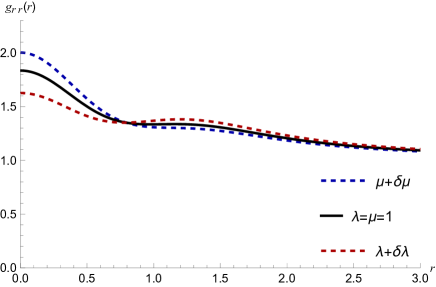
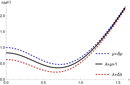
The change in metrics due to elastic parameters can be seen in figures 3 and 4. It is interesting to note that, in addition to the radial component, the angular component of the metric is also modified, which is not particularly expected since the geometric shape has angular symmetry. This change is due to the nature of the strain tensor, which, in cylindrical coordinates landau ; soutas2012elasticity , includes changes in even though the displacement vector is only radial.
We also derive approximate expressions valid near the origin (small r). In this case, we have
| (12) |
and
| (13) |
where the constants are given by (58), (59), (60) and (61). Here, it is worth noting that we can define the following term in (7) . So we will have
| (14) |
in which and are the constants redefined by factoring . Rewriting it this way, just as we did in vozmediano1 , we can look at case . So we immediately see that
| (15) |
This will be useful for determining analytical approximations in section III.1.
We will use Greek indices for the curved space and initial Latin indices to denote the apartment space. Let’s consider that there is local Lorentz symmetry, so we can relate the curved metric to the flat Minkowski metric
| (16) |
where the vielbeins satisfy . The flat indices will take the values . A general choice for the vielbein satisfying Eq. (16) has the form
| (17) |
Then we can obtain the connection 1-form by
| (18) |
where the Christoffel symbols are defined as
| (19) |
The results obtained are lengthy, and they can be found in the appendix. Namely, if we do not take into account the contributions of the displacement vectors , the Christoffel symbols (62), (63) and (64) are reduced to those obtained in vozmediano1 , except for the symmetrization factor in (4), i.e., for we have
|
|
(20) |
where here and . For our static case and with and , the curvature can be written in terms of the deformation vector by 65. The analytical expression for is too long and is not very useful. However, it is possible to numerically analyze, in figure 5, the behavior due to variations in Lamé coefficients.
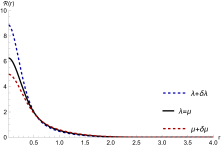
Near the origin, it is important to note again the opposite contributions of and to the curvature. Now we can already adapt the Dirac equation. In particular, we will be interested in the search for stationary states, so we will now determine the Hamiltonian adapted to the geometry of the problem.
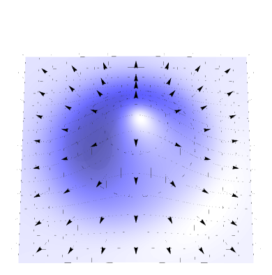
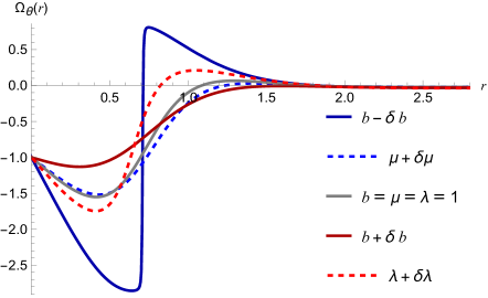
The relationship between effective fields and curvature is a well-known fact in the literature vozmediano1 ; vozmediano2 . Following the approach used in arias1 , we identify the non-zero component of the spin connection by the potential geometric vector vector such that
| (21) |
For different variations of and the relationship is satisfied for . In other words, since in two dimensions the scalar curvature is half the Gaussian curvature , we have that
| (22) |
and this result coincides with (21) applied to and obtained in euclides1 . In work arias1 , Arias obtains the relation , but bases it on the spin connection calculated in vozmediano1 which contains a small algebraic error of a factor of of symmetrization in the product of the Dirac matrices. Absorbing this factor reduces to . But here we use the fact that in two dimensions the scalar curvature is equal to twice the Gaussian curvature.
III Fermion dynamics
Assuming that the spinor is contained in a space of (2+1) dimensions and that, like many similar models vozmediano1 ; arias1 , it has no mass, we obtain
| (23) |
We introduce curvature into the spinor derivative through the covariant derivative . The following representation was adopted for the Dirac matrices , , and . As this is an effective approach, the light speed is replaced by the Fermi speed . Expanding the sum by (23) gives us
| (24) |
where we identify the Dirac Hamiltonian by
| (25) |
The component is null, so we only have contributions from . We have
| (26) |
and we can analyze the behavior of in figure 6.
The curved Dirac matrices can be determined through contractions with vielbeins
| (27) |
so we obtain the following expressions
| (28) | ||||
Using these matrices and the Hamiltonian (26) we get
|
|
(29) |
In particular, we will fix , which ensures that the contributions go to zero for . Then
| (30) |
where we are labeling the term that arises from the spin connection by
| (31) |
Note that acts as a geometric potential in the Hamiltonian. Looking at the expression (26), we can conclude that, for , this term vanishes. This is only true because once arises from the spin connection, this boundary condition is completely sensitive to the choice of vielbeins. For example, if (17) is explicitly of the form , then, even if we fix , there will still be contributions that decrease with , namely . Since the vielbeins define local frames, these contributions are the effects of changes in a non-coordinate basis, so that the effective fields sense these choices. So, the choice guarantees that in the flat case, i.e. , there is no geometric potential and the particle is completely free. Given that we have determined the Hamiltonian, the most natural way to study the effects of both deformations is to look for stationary states euclides1 ; euclides2 ; carlos .
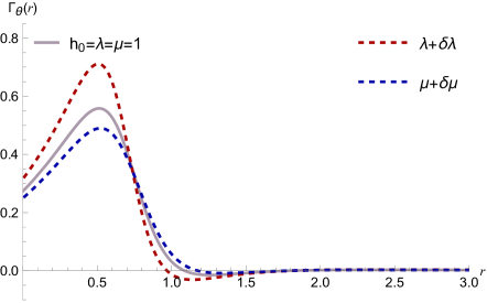
We can see that, for the parameters tested, the potential is attractive near the origin but then becomes repulsive.
III.1 Stationary solutions
We consider a separable solution of the form
| (32) |
such that
| (33) |
Developing this for the Hamiltonian (30), we obtain two coupled equations
| (34) |
in which . To decouple the equations, we can define the operators
| (35) |
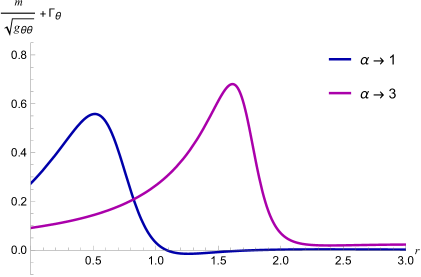
So we can interpret the term as an effective potential and then we notice that, from this perspective, the factor in the first term causes to dominate the behavior of this effective potential, in such a way that the difference between the tested values of became irrelevant. Namely, the behavior is governed by the geometric terms, as shown in figure 8. The factor is always non-zero for , which ensures that the value at the origin is finite.
Thus (33) can be written in compact form by
| (36) |
such that
| (37) |
By multiplying the first by and the second by we can decouple the equations
| (38) |
Developing the first equation, we get
| (39) |
with
| (40) |
Similarly, the equation for is obtained by replacing . In particular, we can define
| (41) |
and
| (42) |
We can call this the effective Fermi velocity; this coincides with the one defined in vozmediano1 . We have also
| (43) |
then . Thus, multiplying (42) by we have
| (44) |
We employ the change on the wave function performed in reference euclides1 of the form , where is given by
| (45) |
in which is a constant. In this way, we can obtain a Klein-Gordon-type expression with an associated squared effective potential. As a result, the new wave function satisfies the equation
| (46) |
and is the effective squared potential and of form
| (47) |
It is worth noting the importance of the function . In fact, the expression in Eq.(45) depends on an integral of the geometric connection. Therefore, can be understood as a kind of geometric Aharonov-Bohm effect, as discussed in furtado ; carlos ; geometricphase ; cone . In order to fix the constant , we consider .
Now let us analyze the behavior of the squared effective potential and the respective wave functions. First, consider far from the bump, whose expression becomes
| (48) |
Accordingly, the Klein-Gordon-like Eq.(46) yields
| (49) |
whose solution is given by
|
|
(50) |
where are Bessel functions of the first kind and are the second kind. To avoid a divergence at the origin, we set . Therefore, the wave function behaves as a free state asymptotically, as expected.
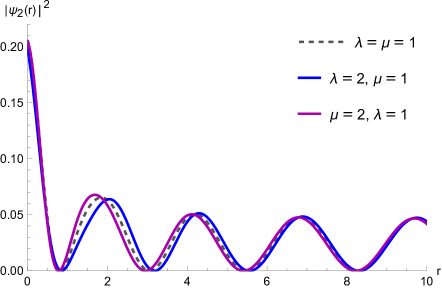
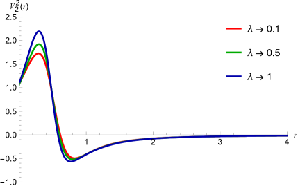
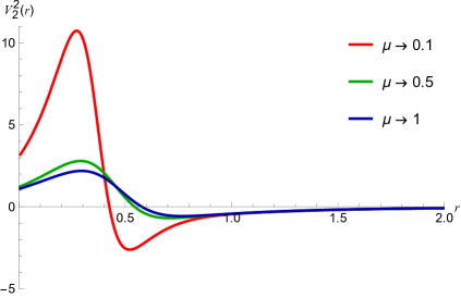
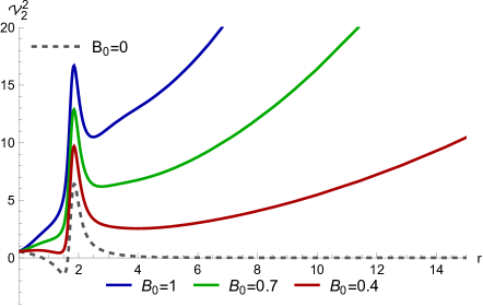
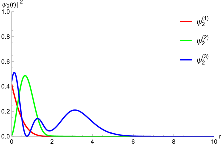
The operator (45) becomes , so (31) implies . Due to the complexity of the squared effective potential, we numerically solved equation 46. The corresponding probability densities are shown in figure 10, where the influence of the Lamé coefficients can be seen; we can see that they tend to change the phase of the wave functions near the origin. Note that the squared effective potential, in figures 11 and 12, is finite and attractive around the origin. Moreover, it has a finite barrier displayed from the origin, and it vanishes asymptotically.
It should be mentioned that the explicit contributions of the Lamé coefficients appear from the second-order approximations. In particular, the solutions are in terms of Heun functions birkandan2008examples , which are more complicated than Bessel functions.
IV External magnetic field
After discussing the strain effects on the electronic states, let us now include an external magnetic field. Assuming an uniform field along the axis, the vector potential is given by . In cylindrical coordinates, and yields
| (51) |
The Hamiltonian for the electron under the influence of strain and magnetic field reads
| (52) |
Following the same development as in section III.1, we will obtain the following equation for
| (53) |
with
|
|
(54) |
Where it is clear that the only change concerning (41) is the inclusion of terms due to the external field in the potential . That is
| (55) |
where
| (56) |
So the Klein-Gordon equation (46) in the presence of an external field is
| (57) |
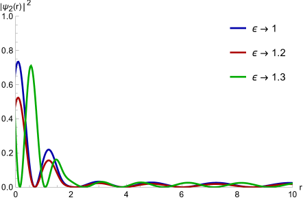
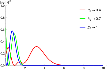
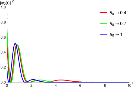
with . So it is immediately clear that, unlike , does not change the holonomy operator (45). This is consistent with their distinct physical origins. We can determine a potential vector . Following euclides1 , we see that the presence of the external field affects the asymptotic limit of the potentials, while preserving the disturbances due to curvature near the origin. In particular, it is clear that when we turn off the external field, the potentials return to those obtained previously, as can be seen in figure 14. Figure 16 shows how the field changes the densities of states.
V Conclusions and Perspectives
In this work, we analyzed the effects of a localized Gaussian deformation on massless Dirac fermions confined to a curved surface, incorporating both in-plane and out-of-plane displacements via elasticity theory. We demonstrated that in-plane strain alters not only the radial component but also the angular part of the surface metric, revealing nontrivial contributions to the spin connection and curvature. These strain-induced modifications were shown to affect the fermionic density of states, with the Lamé coefficients playing a significant role in modulating the effective potential. Analytical and numerical results confirmed the emergence of localized states around the deformation, governed by a geometric potential linked to the spinor holonomy. Upon the application of an external magnetic field, the effective potential exhibits confining behavior at large distances, leading to the formation of Landau levels that localize near the bump. Our analysis reveals a spin-strain coupling mechanism, evidenced by the angular dependence of the metric and the appearance of Heun-type solutions. Future work may explore scattering processes and transport phenomena associated with these geometric potentials using methods such as the Born approximation.
We investigate the effects of a Gaussian deformation taking into account the explicit contributions of in-plane displacements using elasticity theory. We were able to observe that the introduction of the vector proposed by Arias and collaborators arias1 leads to the appearance of angular contributions in the strain tensor, such that the surface metric is not only changed in the radial component vozmediano1 . In fact, non-linear contributions to appear in both the spatial components and . In addition, the explicit use of the vectors induces the appearance of the Lamé constants and , which are associated with the structure of the lattices intrinsically, as discussed in katsnelson , as opposed to the purely geometric perturbations . We conclude that the Lamé constants produce changes in the curvature, and therefore in the effective field, and consequently alter the densities of states of the fermions confined to the surface. Using this approach, we obtained analytical and numerical solutions. In both cases, we observed a shift in the densities of states towards the localized perturbation, as previously observed in other geometric configurations euclides1 ; yecsiltacs2018dirac ; watanabe2015electronic ; bueno2012landau ; diracplanar . In particular, near the origin, we see a behavior mapped by Bessel functions, which is expected due to the cylindrical symmetry of the Gaussian. By the squared effective potential (47) we can see that the metric terms are coupled with the angular momentum terms, which indicates a spin-strain coupling. In fact, for higher orders of we obtain analytical solutions with joint factors of , , and . These solutions remain in terms of Heun’s hypergeometric functions. In general, Heun functions tend to appear in physics problems involving more complex or broken symmetries; the appearance of these functions is particularly interesting as they usually describe disturbances in ideal symmetries birkandan2017quantum ; birkandan2008examples . We have also added an external magnetic field and just as in ref. euclides1 , when we introduce an external magnetic field, we observe that the explained introduction of does not alter the fact that the Landau levels also shift towards the perturbation. In fact they are concentrated in this region, which is where the density of these states is greatest. It was also possible to observe that, since the effective potential is obtained by corrections to the parallel transport of the spinor , every contribution can be absorbed in a holonomy operator, as can be seen in (45) which acts as a geometric phase on a new function in a similar way to an Aharonov-Bohm phase. For future works, it would also be interesting to study the scattering associated with the potentials analyzed in this work. In particular, as seen in section (III), a good way of evaluating the scattering cross section would be to apply the Born-Oppenheimer approximation watanabe2015electronic .
VI Acknowledgments
Samuel B. B. Almeida thanks to Coordenação de Aperfeiçoamento de Pessoal de Nível Superior (CAPES). J. E. G. Silva thanks the Conselho Nacional de Desenvolvimento Científico e Tecnoloógico (CNPq), grant nº 304120/2021-9. C. A. S. Almeida is supported by grant No. 309553/2021-0 (CNPq/PQ) and by Project UNI-00210-00230.01.00/23 (FUNCAP).
CONFLICTS OF INTEREST/COMPETING INTEREST
The authors declared that there is no conflict of interest in this manuscript.
DATA AVAILABILITY
No data was used for the research described in this article.
References
- (1) A. K. Geim, Science, v. 324, (2009) 1530.
- (2) A. Kara et al, Surf. Sci. Rep. 67, 1, (2012).
- (3) A. Carvalho, M. Wang, X. Zhu, A. S. Rodin, H. Su, and A. H. Castro Neto, Nat. Rev. Mater. 1, 1–16 (2016).
- (4) G. H. Liang et al., Phys. Rev. A 98, 062112 (2018).
- (5) A. Shitade, E. Minamitani, New J. Phys. 22, 113023 (2020).
- (6) O. O. Jerjemko, L. S. Brizhik, and V. M. Loktjev, Ukrayins’ kij Fyizichnij Zhurnal (Kyiv) 64, 460–472 (2019).
- (7) C. Si, Z. Sun, F. Liu, Nanoscale 8, 6, 3207 (2016).
- (8) I.Y. Sahalianov, T.M. Radchenko, V.A. Tatarenko, G. Cuniberti, Y.I. Prylutskyy, J. Appl. Phys. 126, 5 (2019).
- (9) A. Gallerati, Phys. Scr. 97, 6, 064005 (2022).
- (10) A. Sepehri, R. Pincak, A.F. Ali, Eur. Phys. J. B 89, 1 (2016).
- (11) A. K. Geim, K. S. Novoselov, Nat. Mat. 6, 183 (2007).
- (12) M. I. Katsnelson, Graphene: Carbon in two dimensions, Cambridge University Press (2012).
- (13) M. A. H. Vozmediano, M. I. Katsnelson, F. Guinea, Phys. Rep. 496, 109 (2010).
- (14) A. H. Castro Neto, F. Guinea, N. M. R. Peres, K. S. Novoselov, and A. K. Geim, Rev. Mod. Phys. 81, 109 (2009).
- (15) K. S. Novoselov et al., Nature 438, 197 (2005).
- (16) V. M. Villalba, A. Rincón Maggiolo, Eur. Phys. J. B 22, 31 (2001).
- (17) C. Bena, G. Montambaux, New J. Phys. 11, 095003 (2009).
- (18) V. M. Pereira, A. H. Castro Neto, N. M. R. Peres, Phys. Rev. B 80, 045401 (2009).
- (19) I. Nikiforov, E. Dontsova, R. D. James, T. Dumitrică, Phys. Rev. B 89, 155437 (2014).
- (20) R. Ribeiro, V. M. Pereira, N. M. R. Peres, P. Briddon, and A. C. Neto, New Journal of Physics 11, 115002 (2009).
- (21) J. L. Manes, F. de Juan, M. Sturla, and M. A. H. Vozmediano, Phys. Rev. B 88, 155405 (2013).
- (22) N. D. Birrell, P. C. W. Davies, Quantum Fields in Curved Space, Cambridge University Press (1984).
- (23) F. de Juan, A. Cortijo, M. A. H. Vozmediano, Phys. Rev. B 76, 165409 (2007).
- (24) F. de Juan, M. Sturla, M. A. H. Vozmediano, Phys. Rev. Lett. 108, 227205 (2012).
- (25) C. Furtado, F. Moraes, A. M. de M. Carvalho, Phys. Lett. A 372, 5368 (2008).
- (26) V. Atanasov, A. Saxena, Phys. Rev. B 92, 035440 (2015).
- (27) M. Watanabe, H. Komatsu, N. Tsuji, H. Aoki, Phys. Rev. B 92, 205425 (2015).
- (28) V. Atanasov, A. Saxena, Phys. Rev. B 81, 205409 (2010).
- (29) K. Flouris, M. M. Jimenez, H. J. Herrmann, Phys. Rev. B 105, 235122 (2022).
- (30) Ö. Yeşiltaş, Adv. High Energy Phys. 2018, 6891402 (2018).
- (31) M. Burgess, B. Jensen, Phys. Rev. A 48, 3, 1861 (1993).
- (32) F.T. Brandt, J.A. Sanchez-Monroy, Phys. Let. A 380, 38, 3036 (2016).
- (33) E. Arias, A. R. Hernández, C. Lewenkopf, Phys. Rev. B 92, 245110 (2015).
- (34) L. D. Landau, E. M. Lifshitz, R. J. Atkin, N. Fox, The Theory of Elasticity, in Physics of Continuous Media, CRC Press, pp. 167–178 (2020).
- (35) R. W. Soutas-Little, Elasticity, Courier Corporation (2012).
- (36) F. de Juan, J. L. Mañes, M. A. H. Vozmediano, Phys. Rev. B 87, 165131 (2013).
- (37) J. E. G. Silva, Ö. Yeşiltaş, J. Furtado, A. A. Araújo Filho, Eur. Phys. J. Plus 139, 762 (2024).
- (38) Ö. Yeşiltaş, J. Furtado, J. E. G. da Silva, Eur. Phys. J. Plus 137, 1–12 (2022).
- (39) T. Birkandan and M. Horta, EAS Publications Series 30, 265–268 (2008).
- (40) L. N. Monteiro, C. A. S. Almeida, J. E. G. Silva, Phys. Rev. B 108, 115436 (2023).
- (41) F. de Juan, A. Cortijo, María A. H. Vozmediano, A. Cano, Nature Physics 7, 810 (2011).
- (42) P. Lammert and V. Crespi, Phys. Rev. lett. 85, 5190 (2000).
- (43) M. J. Bueno, C. Furtado, and A. M. de M. Carvalho, Eur. Phys. J. B 85, 1–5 (2012).
- (44) C. Ho and V. R. Khalilov, Phys. Rev. A 61, 032104 (2000).
- (45) T. Birkandan, M. Hortaçsu, Reports on Mathematical Physics 79, 81–87 (2017).
Appendix A Appendix
By expanding the metrics (10) and (11) in second order in , the Lamé coefficients and geometric parameters of the Gaussian can be absorbed into
| (58) |
| (59) |
| (60) |
| (61) |
The corrections to the parallel transport of the spinor are introduced into the spin connection via the following Christoffel symbols
|
|
(62) |
|
|
(63) |
|
|
(64) |
We can immediately see the algebraic complexity that naturally requires numerical treatment. In particular, it is more insightful to write the disturbances in terms of the displacement vector , as we can see in the following curvature case
|
|
(65) |