Online Knowledge Distillation with Reward Guidance

Abstract

This work studies knowledge distillation (KD) for large language models (LLMs) through preference optimization. We propose a reward-guided imitation learning framework for sequential KD, formulating a min-max optimization problem between the policy and reward model (RM) to minimize the performance gap between the student and teacher policies. Specifically, the reward optimization is constrained to achieve near-optimality within a confidence set for preference alignment. For preference data construction, we explore both offline and online preference-based KD. Additionally, we reformulate the RM using the $Q$-value function and extend the framework to white-box KD, where the teacher policy’s predicted probabilities are accessible. Theoretical analysis and empirical results demonstrate the effectiveness of the proposed framework.

1 Introduction

Large language models (LLMs) such as GPT-4 achiam2023gpt and PaLM anil2023palm have demonstrated impressive capabilities across a wide range of natural language processing (NLP) tasks. Their strong generalization performance is largely attributed to large-scale pretraining and increased model capacity. However, these benefits come at the cost of substantial computational and memory demands, which pose significant challenges for real-world deployment, particularly in resource-constrained settings.

To address these challenges, knowledge distillation (KD) hinton2015distilling has become a widely adopted technique to compress large teacher models into smaller, more efficient student models, while aiming to preserve much of the teacher’s performance. KD methods can be broadly categorized into black-box and white-box approaches, depending on the accessibility of the teacher model’s internal outputs. In black-box KD, the student learns by mimicking the teacher’s outputs using maximum likelihood estimation (MLE) kim2016sequence . In white-box KD, the student has access to the teacher’s output distributions, allowing for more informative training through distribution matching hinton2015distilling ; lin2020autoregressive ; wen2023f ; gu2023minillm ; agarwal2024policy .

Despite their success, existing KD methods face two major challenges. First, the large capacity gap between teacher and student models makes it difficult for the student to accurately replicate the teacher’s outputs, particularly in white-box KD. Second, the teacher’s outputs may themselves be suboptimal for specific downstream tasks, making it undesirable to blindly mimic them.

To overcome these limitations, we propose a novel preference-based knowledge distillation (PbKD) framework as shown in Figure 1. Instead of directly cloning the teacher’s behavior, PbKD formulates KD as a reward-guided imitation learning problem. Our method optimizes the performance gap between the student and teacher policies through a min-max game between the student and a reward model (RM). The RM is constrained within a confidence set constructed from preference data and is optimized to maximize the distinguishability between the student and teacher, guiding the student to improve accordingly.

We further develop an online PbKD variant that iteratively augments the preference dataset with new samples collected from the evolving student policy, enabling continual refinement of the RM and more accurate alignment. In the white-box setting, we extend PbKD by reformulating the RM using $Q$-functions to more effectively leverage the teacher’s output probabilities.

We provide theoretical guarantees for both the offline and online settings. For offline PbKD, we derive a suboptimality bound with a convergence rate of $\mathcal{O}(\sqrt{\log(N/\delta)/N})$, and for online PbKD, we prove a regret bound of order $\mathcal{O}(\sqrt{T\log T\log(T/\delta)})$, where $N$ is the number of preference samples, $d$ is the feature dimension, $T$ is the number of iterations, and $\delta$ is the confidence level. Extensive empirical evaluations across five black-box and five white-box KD benchmarks confirm the effectiveness of our approach, outperforming prior methods.

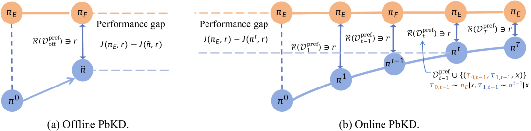
Figure 1: We formulate reward-guided imitation learning as the optimization of the performance gap between the teacher policy $\pi_{E}$ and the student policy $\hat{\pi}$, defined as $\hat{\pi}:=\mathop{\arg\min}_{\pi}\max_{r}J(\pi_{E},r)-J(\pi,r)$ (Eq. (3)). In the offline PbKD setting, a pre-collected preference dataset is used to construct a confidence set for constraining the reward model with MLE, i.e., $r\in\mathcal{R}(\mathcal{D}^{\rm pref}_{\rm off})$ (Algorithm 1). In the online PbKD setting, new preference data are iteratively collected from the current student policy and incorporated into the confidence set, resulting in time-dependent constraints: $r\in\mathcal{R}(\mathcal{D}^{\rm pref}_{t})$ at each iteration $t\in\{1,2,\ldots,T\}$ (Algorithm 2).

2 Related Work

Black-Box Knowledge Distillation. Black-box knowledge distillation (KD) has emerged as a practical solution for compressing large language models (LLMs) like GPT-4 brown2024gpt , Claude 3 anthropic2024claude3 , and Gemini (Google, 2023) into smaller, more efficient student models. Black-box KD leverages only the output responses of proprietary APIs. Recent efforts such as Alpaca taori2023alpaca , Vicuna chiang2023vicuna , and Orca mukherjee2023orca have explored using these responses as supervision to transfer capabilities like reasoning, tool use, and code generation. Techniques include prompting LLMs to generate Chain-of-Thought (CoT) explanations hsieh2023distilling ; wang2023selfinstruct rationale-based reasoning liu2023tinygsm , or code-language pairs azerbayev2023explicit , which are then used to fine-tune smaller models. These approaches demonstrate the potential of black-box LLMs as data generators to train open-source alternatives without requiring access to their internal weights or training data.

White-Box Knowledge Distillation. White-box knowledge distillation (KD) builds upon the classical KD framework introduced by Hinton et al. hinton2015distilling , where the student model learns from the soft predictions of a larger teacher model. This paradigm has been widely applied to compress large pre-trained language models (PLMs), with early work focusing on logits and intermediate features jiao2020tinybert ; sun2019patient ; wang2020minilm . Subsequent methods extended KD to sequence generation tasks, including machine translation and summarization, by aligning entire output distributions chen2020distilling ; wang2021selective . Recent efforts target large language models (LLMs) specifically, exploring divergence-based objectives such as KL, reverse KL (RKL), and Jensen-Shannon (JS) divergence for auto-regressive generation wen2023f ; agarwal2024policy ; gu2023minillm . For instance, Gu et al. gu2023minillm introduced a policy gradient method to reduce RKL variance, while Ko et al. ko2024distillm proposed an efficient skew-divergence-based technique. Additionally, moment-matching and step-wise supervision have gained attention for better aligning generation dynamics jiaadversarial . These works reveal the limitations of traditional divergence objectives and highlight the need for more adaptive and data-efficient strategies in white-box KD for LLMs.

Preference-based Knowledge Distillation. While knowledge distillation (KD) has been extensively studied for large language models (LLMs), relatively few efforts have explored the use of preference optimization to guide the distillation process, aiming to align student models with human preferences. Recent works on preference-based knowledge distillation (PbKD) include li2024direct ; zhang2024plad ; chen2024knowledgedistillationblackboxlarge , where a preference loss is incorporated—typically using pairwise comparisons between teacher and student outputs—alongside the conventional maximum likelihood estimation (MLE) loss used in behavior cloning. Notably, Li et al. li2024direct and Chen et al. chen2024knowledgedistillationblackboxlarge focus on black-box settings, whereas Zhang et al. zhang2024plad propose a method that falls under white-box KD. In contrast to these approaches, we propose a more general PbKD framework grounded in imitation learning, applicable to both black-box and white-box scenarios. Our improvements stem from a more robust min-max optimization framework with an online, iterative training scheme that enhances preference alignment and training stability.

3 Problem Formulation

In this section, we formulate sequential knowledge distillation as an imitation learning problem for language generation. Specifically, we consider language generation as a finite-horizon, time-independent sequence-to-sequence decision-making task. Given an input prompt $x\in\mathcal{X}$, the policy generates an output sequence $y=\{y_{1},\ldots,y_{H}\}$ under an episodic Markov Decision Process (MDP), defined by the tuple $(\mathcal{S},\mathcal{A},T,r^{*})$. Here, $\mathcal{S}=\{s_{h}\}_{0\leq h\leq H}$ denotes the state space consisting of output prefixes $s_{h}=y_{\leq h}$, and $\mathcal{A}=\{a_{h}\}_{0\leq h\leq H-1}$ denotes the action space corresponding to predicted tokens $a_{h}=y_{h+1}$. We assume a deterministic state-transition function $T$ in sequence generation, where each action deterministically advances the state.

Given a policy $\pi$, the prediction of the next action at a state $s$ is modeled as a probability distribution $\pi(\cdot\mid s)$ over $\mathcal{A}$. Starting from an initial state (i.e., prompt) $x\sim d_{0}$, a trajectory is generated as $(a_{0},s_{1},a_{1},\ldots,s_{H-1},a_{H-1},s_{H})\sim\pi\mid x$. The value function of policy $\pi$ with respect to a RM $r$ is defined as the expected cumulative reward over the episode: $V^{\pi}(x)=\mathbb{E}_{\tau\sim\pi\mid x}\left[\sum_{h=0}^{H-1}\gamma^{h}r(s_{h},a_{h})\right]$, where $\gamma\in[0,1]$ is a discount factor. The overall performance of the policy $\pi$ under RM $r$ is then given by the expected value over the input distribution $d_{0}$: $J(\pi,r)=\mathbb{E}_{x\sim d_{0}}\left[V^{\pi}(x)\right]$.

Preference Learning. Given a RM $r$, the preference probability over a binary feedback $o\in\{0,1\}$ for a trajectory pair $(\tau_{0},\tau_{1})$ conditioned on an input $x$ is modeled using the Bradley-Terry-Luce (BTL) formulation:

$$\mathbb{P}_{r}(\tau_{0}\succ\tau_{1}\mid x)=\mathbb{P}_{r}(o=1\mid x,\tau_{0},\tau_{1})=\sigma\left(r(x,\tau_{0})-r(x,\tau_{1})\right),$$ (1)

where $r(x,\tau)=\sum_{h=0}^{H-1}\gamma^{h}r(s_{h},a_{h})$ denotes the cumulative discounted reward of the trajectory $\tau=(s_{1},a_{1},\ldots,s_{H-1},a_{H-1},s_{H})$ conditioned on input $x$, and $\sigma(\cdot)$ is the sigmoid function $\sigma(x)=1/(1+\exp(-x))$.

We assume the existence of a ground-truth reward model $r^{*}$ that induces the true preference distribution, i.e., $\mathbb{P}(\tau_{0}\succ\tau_{1}\mid x)=\mathbb{P}_{r^{*}}(o=1\mid x,\tau_{0},\tau_{1})$.$\mathbb{P}(\tau_{0}\succ\tau_{1}\mid x)=\mathbb{P}_{r^{*}}(o=1\mid x,\tau_{0},\tau_{1})$. To evaluate the discrepancy between a candidate RM $r\in\mathcal{G}_{r}$ and the true model $r^{*}$, we define the maximum likelihood estimation (MLE) loss for a single preference instance as:

$$\ell_{r}(o;x,\tau_{0},\tau_{1})=\begin{cases}\frac{1}{2}\log\frac{\mathbb{P}_{r}(o\mid x,\tau_{0},\tau_{1})}{\mathbb{P}_{r^{*}}(o\mid x,\tau_{0},\tau_{1})},&\text{if }\mathbb{P}_{r^{*}}(o\mid x,\tau_{0},\tau_{1})\neq 0\\ 0,&\text{otherwise}\end{cases}$$ (2)

The empirical MLE objective over a dataset of $N$ preference-labeled samples $\mathcal{D}^{\text{pref}}=\{(o_{n};x_{n},\tau_{0,n},\tau_{1,n})\}_{n=1}^{N}$ is given by: $L_{r}(\mathcal{D}^{\text{pref}})=\sum_{n=1}^{N}\ell_{r}(o_{n};x_{n},\tau_{0,n},\tau_{1,n})$. We denote by $\mathcal{L}_{r}=\{\ell_{r}:r\in\mathcal{G}_{r}\}$ the class of MLE objective functions corresponding to the reward model function class $\mathcal{G}_{r}$.

Definition 1 ($\epsilon$-Bracketing Number of the MLE Class $\mathcal{L}_{r}$).

Let $\mathcal{L}_{r}$ be the class of MLE objective functions. A pair $(\ell_{1},\ell_{2})$ with $\ell_{1},\ell_{2}\in\mathcal{L}_{r}$ is called an $\epsilon$-bracket if it satisfies:

• $\ell_{1}(o;x,\tau_{0},\tau_{1})\leq\ell_{2}(o;x,\tau_{0},\tau_{1})$ for all preference samples $(o;x,\tau_{0},\tau_{1})$;

• The $L_{1}$-distance between the two functions is bounded as $\left\|\ell_{1}-\ell_{2}\right\|_{1}\leq\epsilon$.

The $\epsilon$-bracketing number of $\mathcal{L}_{r}$ with respect to the $L_{\infty}$ norm, denoted by $\mathcal{N}_{[]}(\epsilon,\mathcal{L}_{r},L_{\infty})$, is the minimal number of such brackets $\{(\ell_{1,n},\ell_{2,n})\}_{n=1}^{N}$ required to cover $\mathcal{L}_{r}$, in the sense that for every $\ell\in\mathcal{L}_{r}$, there exists an index $n\in[N]$ such that $\ell_{1,n}(o;x,\tau_{0},\tau_{1})\leq\ell(o;x,\tau_{0},\tau_{1})\leq\ell_{2,n}(o;x,\tau_{0},\tau_{1}),\quad\forall(o;x,\tau_{0},\tau_{1})$.

In the following PAC analysis, we assume that the reward function class $\mathcal{G}_{r}$ satisfies three conditions: realizability, linearity, and boundedness.

Assumption 1 (Realizability).

We assume the reward class is realizable, i.e., the ground-truth reward function $r^{*}$ lies in the function class: $r^{*}\in\mathcal{G}_{r}$.

Assumption 2 (Linearity and Boundedness).

We assume the reward function is linearly parameterized as $r_{\theta}(x,\tau)=\theta^{\top}\phi(x,\tau)$, $\phi:(x,\tau)\mapsto\phi(x,\tau)\in\mathbb{R}^{d}$ is a fixed feature extractor. Furthermore, we assume the features and parameters are bounded such that $\|\phi(x,\tau)\|_{2}\leq 1$ for all $(x,\tau)$ and $\|\theta\|_{2}\leq B$ for some constant $B>0$.

Proposition 1 (Bracketing Number of the MLE Loss Class zhanprovable ).

Under Assumption 2, for any $\epsilon\leq 1$, the $\epsilon$-bracketing number of the MLE objective function class $\mathcal{L}_{r}$ with respect to the $L_{\infty}$ norm satisfies: $\log\mathcal{N}_{[]}(\epsilon,\mathcal{L}_{r},L_{\infty})\leq\mathcal{O}\left(d\log\frac{B}{\epsilon}\right)$.

Reward-Guided Imitation Learning. We consider an imitation learning formulation for knowledge distillation, where the goal is to learn a student policy $\pi\in\Pi$ that closely imitates an expert (i.e., teacher) policy $\pi_{E}$. Formally, we aim to minimize the worst-case performance gap between the student and expert policies over a set of plausible reward models inferred from preference data:

$$\hat{\pi}=\mathop{\arg\min}_{\pi\in\Pi}\max_{r\in\mathcal{R}(\mathcal{D}^{\rm pref})}J(\pi_{E},r)-J(\pi,r),$$ (3)

where the reward confidence set $\mathcal{R}(\mathcal{D}^{\rm pref})\subseteq\mathcal{G}_{r}$ is constructed via the maximum likelihood estimation (MLE) on the preference dataset $\mathcal{D}^{\rm pref}$:

$$\mathcal{R}(\mathcal{D}^{\rm pref})=\left\{r\in\mathcal{G}_{r}:L_{r}(\mathcal{D}^{\rm pref})\geq\max_{r\in\mathcal{G}_{r}}L_{r}(\mathcal{D}^{\rm pref})-\zeta\right\}$$ (4)

with $\zeta\geq 0$ being a slack parameter controlling the confidence radius.

The resulting objective in Eq. (3) constitutes a min-max optimization problem between the student policy and an uncertain reward function. The inner maximization identifies the least favorable reward model $r\in\mathcal{R}(\mathcal{D}^{\rm pref})$ that maximizes the performance gap, thereby encouraging robustness to reward uncertainty. Rather than simply using the MLE estimate $\hat{r}=\arg\max_{r\in\mathcal{G}_{r}}L_{r}(\mathcal{D}^{\rm pref})$, this approach penalizes student policies that do not generalize well under plausible alternative reward functions, leading to a distributionally robust formulation of imitation learning.

In what follows, we introduce different instantiations of this reward-guided imitation learning framework for knowledge distillation, categorized into three settings:

1. Offline preference-based knowledge distillation (offline PbKD; Section 4), which uses a fixed offline preference dataset;

2. Online preference-based knowledge distillation (online PbKD; Section 5), where preferences are collected and incorporated during training;

3. Moment-matching PbKD (Section 6), which leverages the preference difference lemma (PDL) and reformulates the objective in terms of $Q$-function matching.

All theoretical results are supported with detailed proofs provided in the Appendix.

4 Offline Preference-based Knowledge Distillation

4.1 Algorithm

In the offline PbKD setting, we are given a fixed offline preference dataset $\mathcal{D}_{\rm off}^{\rm pref}=\{(o_{n};x_{n},\tau_{0,n},\tau_{1,n})\}_{n=1}^{N}$, where each input $x_{n}$ is sampled i.i.d. from a distribution $d_{0}$, and the corresponding trajectory pair $(\tau_{0,n},\tau_{1,n})$ is independently sampled from two policies $\mu_{0}(\cdot\mid x_{n})$ and $\mu_{1}(\cdot\mid x_{n})$, respectively. The preference label $o_{n}\in\{0,1\}$ is sampled according to the ground-truth preference distribution $\mathbb{P}_{r^{*}}(o_{n}\mid x_{n},\tau_{0,n},\tau_{1,n})$, which is typically derived from human annotations christiano2017deep ; ziegler2019fine ; stiennon2020learning ; ouyang2022training or high-quality AI feedback guo2024direct ; pang2024iterative ; cen2024value ; cui2024ultrafeedback .

We present the algorithm for offline preference-based knowledge distillation (offline PbKD) in Algorithm 1. Given the offline preference dataset $\mathcal{D}_{\rm off}^{\rm pref}$, our goal is to obtain the student policy $\hat{\pi}$ that minimizes the worst-case performance gap with respect to the expert policy $\pi_{E}$, following the reward-guided imitation learning objective in Eq. (3).

To avoid directly solving the constrained optimization problem involving the reward confidence set, we adopt a Lagrangian relaxation approach. By introducing a Lagrange multiplier $\beta\geq 0$, we convert the original constrained problem into the following unconstrained bi-level optimization formulation:

$$\hat{\pi}=\mathop{\arg\min}_{\pi\in\Pi}\max_{r\in\mathcal{G}_{r}}J(\pi_{E},r)-J(\pi,r)+\beta L_{r}(\mathcal{D}_{\rm off}^{\rm pref}),$$ (5)

where the reward model $r$ is simultaneously optimized to maximize the likelihood of the observed preferences via the MLE objective $L_{r}(\mathcal{D}_{\rm off}^{\rm pref})$, while inducing the largest performance gap between the student and expert. This encourages the student policy to be robust against plausible reward functions supported by the offline preference data.

Input: Offline preference dataset $\mathcal{D}_{\rm off}^{\rm pref}=\{(0_{n};x_{n},\tau_{0,n},\tau_{1,n})\}_{n=1}^{N}$, student policy class $\Pi$, teacher policy $\pi_{E}$, input distribution $d_{0}$.

Compute the best policy under constraints on offline confidence set:

$$\hat{\pi} =\mathop{\arg\min}_{\pi\in\Pi}\max_{r\in\mathcal{R}(\mathcal{D}^{\rm pref}_{\rm off})}J(\pi_{E},r)-J(\pi,r)$$ (6)

$${s.t.}\ \mathcal{R}(\mathcal{D}^{\rm pref}_{\rm off}) =\left\{r\in\mathcal{G}_{r}:L_{r}(\mathcal{D}^{\rm pref}_{\rm off})\geq\max_{r\in\mathcal{G}_{r}}L_{r}(\mathcal{D}^{\rm pref}_{\rm off})-\zeta\right\}$$ (7)

Output: The optimized student policy $\hat{\pi}$.

Algorithm 1 Offline PbKD

4.2 Learning Guarantee

We evaluate the quality of the learned student policy $\hat{\pi}$ by its suboptimality under the ground-truth reward model $r^{*}$. Specifically, we consider the performance gap between $\hat{\pi}$ and the optimal policy $\pi^{*}=\mathop{\arg\max}_{\pi\in\Pi}J(\pi,r^{*})$, defined as: $J(\pi^{*},r^{*})-J(\hat{\pi},r^{*})$. This quantity characterizes how far the learned policy is from the best achievable performance under the true reward.

The following theorem provides a learning guarantee for offline PbKD, bounding the suboptimality of $\hat{\pi}$ in terms of the quantity of offline preference data and the functional complexity.

Definition 2 (Concentrability Coefficient for Offline Preference).

The concentrability coefficient w.r.t. a RM class $\mathcal{G}_{r}$, the teacher policy $\pi_{E}$ and the optimal student policy $\pi^{*}$ is defined as:

$$C_{r}(\mathcal{G}_{r},\pi_{E},\pi^{*})=\sup_{r\in\mathcal{G}_{r}}\frac{\mathbb{E}_{x\sim d_{0},\tau_{0}\sim\pi_{E}\mid x,\tau_{1}\sim\pi^{*}\mid x}\left[r^{*}(\tau_{0})-r^{*}(\tau_{1})-\left(r(\tau_{0})-r(\tau_{1})\right)\right]}{\sqrt{\mathbb{E}_{x\sim d_{0},\tau_{0}\sim\mu_{0}\mid x,\tau_{1}\sim\mu_{1}\mid x}\left[|r^{*}(\tau_{0})-r^{*}(\tau_{1})-\left(r(\tau_{0})-r(\tau_{1})\right)|^{2}\right]}}$$ (8)

The concentrability coefficient, which has also been adopted in the literature chen2019information ; songhybrid ; zhanprovable ; ye2024online , is defined as an information-theoretic ratio that quantifies the mismatch between the distribution of the preference data and the distributions induced by the teacher policy $\pi_{E}$ and the optimal student policy $\pi^{*}$. It captures this discrepancy in terms of the reward differences between positive and negative preference-labeled outputs. Based on the definition of concentrability coefficient, we derive a suboptimality bound as follows.

Theorem 1 (Suboptimality).

For any $\delta\in(0,1]$, given an offline preference dataset with a size of $N$, and let $\zeta=\mathcal{O}\left(\sqrt{\log(\mathcal{N}_{[]}(\epsilon,\mathcal{L}_{r},L_{\infty})/\delta)/N}\right)$, then under Assumption 1, and assuming that $\|1/\sigma(1-\sigma)\|_{\infty}\leq\kappa$, for some constant $\kappa\geq 0$, we have with probability at least $1-\delta$:

$$J(\pi^{*},r^{*})-J(\hat{\pi},r^{*})\leq\mathcal{O}\left(\kappa C_{r}(\mathcal{G}_{r},\pi_{E},\pi^{*})\sqrt{\frac{\log(\mathcal{N}_{[]}(1/N,\mathcal{L}_{r},L_{\infty})/\delta)}{N}}\right)$$

If we further assume that Assumption 2 holds, we have

$$J(\pi^{*},r^{*})-J(\hat{\pi},r^{*})\leq\mathcal{O}\left((1+e^{2B})\left\|\phi(x,\pi_{E})-\phi(x,\pi^{*})\right\|_{\Sigma^{-1}}\sqrt{\frac{d\log(BN)+\log(1/\delta)}{N}}\right),$$

where $\Sigma$ denotes the covariance matrix corresponding to the expected difference between feature vectors of preference pairs, defined as: $\Sigma=\frac{\lambda}{B}I+\mathbb{E}_{x\sim d_{0},\tau_{0}\sim\mu_{0}\mid x,\tau_{1}\sim\mu_{1}\mid x}\left[\left(\phi(x,\tau_{0})-\phi(x,\tau_{1})\right)\left(\phi(x,\tau_{0})-\phi(x,\tau_{1})\right)^{\top}\right]$ given a positive constant $0<\lambda\leq\mathbb{E}_{x\sim d_{0},\tau_{0}\sim\mu_{0}\mid x,\tau_{1}\sim\mu_{1}\mid x}\left[|r^{*}(\tau_{0})-r^{*}(\tau_{1})-\left(r(\tau_{0})-r(\tau_{1})\right)|^{2}\right]$.

Remark 1 (Convergence Rate and Sample Complexity).

Theorem 1 establishes that Algorithm 1 achieves a convergence rate of $\mathcal{O}(\sqrt{\log(N/\delta)/N})$ for the suboptimality gap of the student policy, where $N$ is the number of preference samples, and $\delta$ is the confidence level. This implies a sample complexity of $N\geq\tilde{\mathcal{O}}\left(\frac{\log(1/\delta)}{\epsilon^{2}}\right)$ to guarantee an $\epsilon$-optimal solution, i.e., $J(\pi^{*},r^{*})-J(\hat{\pi},r^{*})\leq\epsilon$.

5 Online Preference-based Knowledge Distillation

5.1 Algorithm

In contrast to the offline setting, the online paradigm allows for leveraging preference data from both the student and teacher policies throughout the training process. Given that obtaining preference annotations from humans or LLMs can be expensive and time-consuming, we make a simplifying assumption: responses from the teacher policy are always preferred over those from the student policy.

We present the online preference-based knowledge distillation (online PbKD) algorithm in Algorithm 2. At each iteration $t-1\in\{0,2,\ldots,T-1\}$, we collect a the preference-labeled sample $(o_{t-1}=1;x_{t-1},\tau_{0,t-1},\tau_{1,t-1})$, where $x_{t-1}\sim d_{0}$ is drawn from the input distribution, and the trajectory pair $(\tau_{0,t-1},\tau_{1,t-1})$ is generated by sampling from the teacher policy $\pi_{E}(\cdot\mid x_{t-1})$ and the current student policy $\pi^{t-1}(\cdot\mid x_{t})$, respectively.

The reward model is optimized within a confidence set constructed from the preference data collected up to iteration $t$, denoted as $\mathcal{D}_{t}^{\rm pref}=\{(o_{s}=1;x_{s},\tau_{0,s},\tau_{1,s})\}_{s=0}^{t-1}$. Analogous to the offline formulation, we introduce a Lagrangian multiplier $\beta$ to convert the constrained optimization problem into an unconstrained bi-level problem regularized by the MLE objective:

$$\pi^{t}=\mathop{\arg\min}_{\pi\in\Pi}\max_{r\in\mathcal{G}_{r}}J(\pi_{E},r)-J(\pi,r)+\beta L_{r}(\mathcal{D}_{t}^{\rm pref})$$ (9)

Input: (Empty) set $\mathcal{D}^{\rm pref}_{0}$, student policy class $\Pi$, teacher policy $\pi_{E}$, input distribution $d_{0}$.

for $t=1,2,\ldots,T$ do

    Sample an input $x_{t-1}\sim d_{0}$ and trajectories $\tau_{0,t-1}\sim\pi_{E}\mid x_{t-1}$ and $\tau_{1,t-1}\sim\pi^{t-1}\mid x_{t-1}$

    Add the sample into the previous preference set:

    $\mathcal{D}^{\rm pref}_{t}\leftarrow\mathcal{D}^{\rm pref}_{t-1}\cup\{(o_{t-1}=1;x_{t-1},\tau_{0,t-1},\tau_{1,t-1})\}$

    Compute the $t$-iteration best policy under constraints on the $t$-iteration confidence set:

$${\pi}^{t} =\mathop{\arg\min}_{\pi\in\Pi}\max_{r\in\mathcal{R}(\mathcal{D}^{\rm pref}_{t})}J(\pi_{E},r)-J(\pi,r),$$ (10)

$${\rm s.t.}\ \mathcal{R}(\mathcal{D}_{t}^{\rm pref}) =\left\{r\in\mathcal{G}_{r}:L_{r}(\mathcal{D}_{t}^{\rm pref})\geq\max_{r\in\mathcal{G}_{r}}L_{r}(\mathcal{D}_{t}^{\rm pref})-\zeta_{t}\right\}$$ (11)

end for

Output: The sequence of optimized student policy $\{\pi^{t}\}_{t=1}^{T}$.

Algorithm 2 Online PbKD

5.2 Learning Guarantee

We provide a theoretical guarantee for Algorithm 2 by establishing a cumulative regret bound. Specifically, we measure the cumulative performance gap between the sequence of learned student policies and the optimal student policy under the golden reward model $r^{*}$: $\sum_{t=1}^{T}J(\pi^{*},r^{*})-J(\pi^{t},r^{*})$, where the optimal student policy is defined as $\pi^{*}=\mathop{\arg\max}_{\pi\in\Pi}J(\pi,r^{*})$.

This cumulative regret quantifies how far the iteratively learned policies $\{\pi^{t}\}_{t=1}^{T}$ are from the optimal policy in hindsight, and serves as a key metric for evaluating the efficiency and effectiveness of the online preference-based knowledge distillation process.

Definition 3 (Concentrability Coefficient for Online Preference).

The concentrability coefficient for online preference at iteration $t\in\{1,2,\ldots,T\}$ is defined as:

$$C_{r}^{t}(\mathcal{G}_{r},\pi_{E},\pi^{*})=\sup_{r\in\mathcal{G}_{r}}\frac{\mathbb{E}_{x\sim d,\tau_{0}\sim\pi_{E}\mid x,\tau_{1}\sim\pi^{*}\mid x}\left[r^{*}(\tau_{0})-r^{*}(\tau_{1})-\left(r(\tau_{0})-r(\tau_{1})\right)\right]}{\sqrt{\sum_{s=0}^{t-1}\mathbb{E}_{x_{s}\sim d_{0},\tau_{0,s}\sim\pi_{E}\mid x,\tau_{1,s}\sim\pi^{s}\mid x}\left[|r^{*}(\tau_{0})-r^{*}(\tau_{1})-\left(r(\tau_{0})-r(\tau_{1})\right)|^{2}\right]}}$$

Theorem 2 (Regret).

For any $\delta\in(0,1]$, let $\zeta_{t}=\mathcal{O}\left(\log(\mathcal{N}_{[]}(1/t,\mathcal{L}_{r},L_{\infty})/\delta)\right)$ for any $t\in\{1,2,\ldots,T\}$ with a maximum iteration number of $T$, then under Assumption 1, we have with probability at least $1-\delta$:

$$\sum_{t=1}^{T}J(\pi^{*},r^{*})-J(\pi^{t},r^{*})\leq\mathcal{O}\left(\kappa\sum_{t=1}^{T}C_{r}^{t}(\mathcal{G}_{r},\pi_{E},\pi^{*})\log\frac{\mathcal{N}_{[]}(1/t,\mathcal{L}_{r},L_{\infty})}{\delta}\right)$$

If we further assume that Assumption 2 holds, we have

$$\sum_{t=1}^{T}J(\pi^{*},r^{*})-J(\pi^{t},r^{*})\leq\mathcal{O}\left((1+e^{2B})\sqrt{d\log(1+TB/d\lambda_{1})\sum_{t=1}^{T}\left(d\log(Bt)+\log(1/\delta)\right)}\right),$$

where $0<\lambda_{1}\leq\mathbb{E}_{x\sim d_{0},\tau_{0}\sim\pi_{E}\mid x,\tau_{1}\sim\pi^{0}\mid x}\left[|r^{*}(\tau_{0})-r^{*}(\tau_{1})-\left(r(\tau_{0})-r(\tau_{1})\right)|^{2}\right]$ denotes a positive constant.

Remark 2 (Convergence Rate and Complexity).

Theorem 2 shows that Algorithm 2 achieves a regret bound in the order of approximately $\mathcal{O}(\sqrt{T\log T\log(T/\delta)})$ in terms of the number of iterations $T$ and the confidence factor $\delta$. This implies that the average regret, defined as $J(\pi^{*},r^{*})-\frac{1}{T}\sum_{t=1}^{T}J(\pi^{t},r^{*})$, decays at a rate of approximately $\mathcal{O}(\sqrt{\log T\log(T/\delta)/T})$. To achieve an $\epsilon$-approximate convergence in average regret, i.e., $\frac{1}{T}\sum_{t=1}^{T}J(\pi^{t},r^{*})\geq J(\pi^{*},r^{*})-\epsilon$ the number of iterations $T$ must satisfy $T\geq\tilde{\mathcal{O}}\left(\frac{\log(1/\delta)}{\epsilon^{2}}\right)$. This establishes the iteration complexity of the online PbKD algorithm for achieving $\epsilon$-optimality in regret.

6 Moment-Matching PbKD

The preference-based knowledge distillation (PbKD) framework proposed in the previous sections can be categorized as black-box knowledge distillation, since it relies solely on the trajectories output by the teacher policy without accessing the token-level probabilities computed by the teacher policy, as commonly done in white-box distillation approaches hinton2015distilling ; wen2023f ; agarwal2024policy ; gu2023minillm .

In this section, we extend the PbKD framework to the white-box setting by leveraging the performance difference lemma (PDL) to reformulate the optimization in Eq. (3) as a dual problem. This leads to our proposed approach: moment-matching preference-based knowledge distillation (MM PbKD).

Proposition 2 (Performance Difference Lemma swamy2021moments ; jiaadversarial ).

Let $Q^{\pi_{E}}_{r}$ denote the $Q$-function under the teacher policy $\pi_{E}$ and reward function $r\in\mathcal{G}_{r}$, defined as $Q^{\pi_{E}}_{r}(s_{h},a_{h})=\mathbb{E}_{\tau\sim\pi_{E}\mid s_{h},a_{h}}\left[\sum_{h^{\prime}=h}^{H-1}\gamma^{h^{\prime}-h}r(s_{h^{\prime}},a_{h^{\prime}})\right]$. Then, the performance difference between the teacher policy $\pi_{E}$ and a student policy $\pi$ under reward $r$ satisfies:

$$J(\pi_{E},r)-J(\pi,r)=\mathbb{E}_{x\sim d_{0},\tau\sim\pi\mid x}\left[\sum_{h=0}^{H-1}\mathbb{E}_{a\sim\pi_{E}(\cdot\mid s_{h})}Q^{\pi_{E}}_{r}(s_{h},a)-Q^{\pi_{E}}_{r}(s_{h},a_{h})\right]$$

We define the class of teacher $Q$-functions induced by $\mathcal{G}_{r}$ as: $\mathcal{G}_{Q_{E}}=\left\{Q^{\pi_{E}}_{r}:r\in\mathcal{G}_{r}\right\}$, where each $f\in\mathcal{G}_{Q_{E}}$ represents a $Q$-function $Q^{\pi_{E}}_{r}$ under some reward model $r$.

Under a deterministic transition assumption, i.e., $T(s_{h+1}\mid s_{h},a_{h})=1$, the Bellman equation gives: $Q^{\pi_{E}}_{r}(s_{h},a_{h})=r(s_{h},a_{h})+\gamma\mathbb{E}_{a^{\prime}\sim\pi_{E}(\cdot\mid s_{h+1})}Q^{\pi_{E}}_{r}(s_{h+1},a^{\prime}).$ Thus, the reward function induced by any $f\in\mathcal{G}_{Q_{E}}$ can be written as: $r(f):=f-\gamma f\circ\pi_{E}$.

Using Proposition 2, the original optimization problem in Eq. (3) can be reformulated as a dual optimization problem:

$$\hat{\pi}=\arg\min_{\pi\in\Pi}\max_{f\in\mathcal{Q}(\mathcal{D}^{\text{pref}})}\mathbb{E}_{x\sim d_{0},\tau\sim\pi\mid x}\left[\sum_{h=0}^{H-1}\mathbb{E}_{a\sim\pi_{E}(\cdot\mid s_{h})}f(s_{h},a)-f(s_{h},a_{h})\right],$$ (12)

where the confidence set $\mathcal{Q}(\mathcal{D}^{\text{pref}})\subset\mathcal{G}_{Q_{E}}$ is constructed using the induced reward $r(f)$ as:

$$\mathcal{Q}(\mathcal{D}^{\text{pref}}):=\left\{f\in\mathcal{G}_{Q_{E}}:L_{r(f)}(\mathcal{D}^{\text{pref}})\geq\max_{f\in\mathcal{G}_{Q_{E}}}L_{r(f)}(\mathcal{D}^{\text{pref}})-\zeta\right\}$$ (13)

This formulation can be interpreted as a moment-matching objective: minimizing the expected discrepancy between (1) the teacher’s expected $Q$-value and (2) the student policy’s realized $Q$-value at each step $h\in\{0,1,\dots,H-1\}$. It naturally lends itself to an on-policy RL algorithm for optimization, such as those used by Swamy et al. swamy2021moments .

Similar to previous sections, we can further instantiate this framework as: Offline MM PbKD, where the confidence set is built using a fixed, pre-collected preference dataset. Online MM PbKD, where preferences are collected dynamically during training. These extensions allow MM PbKD to flexibly adapt to various supervision settings while incorporating white-box information from the teacher.

7 Experiments

We evaluate knowledge distillation using both black-box and white-box LLMs.

7.1 Knowledge Distillation with Black-Box LLMs

We study knowledge distillation from black-box LLMs, where internal information are inaccessible and interaction is limited to API outputs used to train smaller student models.

Experimental Setup. We choose GPT-4 achiam2023gpt as the black-box teacher and initialize the student with LLaMA2 7B touvron2023llama . Training data is sampled from a mix of OpenOrca lian2023openorca and Nectar starling2023 , totaling 100,000 prompts. Evaluation uses diverse benchmarks: BBH suzgun2023challenging , AGIEval zhong2024agieval , ARC-Challenge clark2018think , MMLU hendryckstest2021 , and GSM8K cobbe2021training . Offline preference data is pre-collected by fine-tuning several LLMs on 10,000 samples to generate candidate outputs, ranked by GPT-4 feedback. The reward model (RM) is a linear layer atop a fixed Llama-2-7B. For offline PbKD, parameters are randomly initialized; for online PbKD, pretrained on offline preference data. Online PbKD runs for 5 iterations, each sampling 1,000 prompts to generate preference pairs from the current student and teacher, augmenting the dataset for RM training. Results are averaged over three seeds; details in the Appendix.

Main Results. Table 1 reports results. Our method surpasses the Vanilla Black-Box KD baseline, which directly fine-tunes on teacher outputs, and improves upon Best-of-$N$ sampling stiennon2020learning (with $N=10$) that selects candidates by RM scores. Compared to Proxy-KD chen2024knowledgedistillationblackboxlarge , which uses a white-box proxy model aligned with the black-box teacher, our preference-optimization based min-max formulation achieves better accuracy and robustness. Ablation on online PbKD iterations shows consistent gains over offline-only training, with performance steadily improving as iterations increase—highlighting the benefits of iterative reward-guided distillation.

Table 1: Black-box KD on five datasets. ^∗ indicates that the results are from their original papers. We format the best and the second best results. The results based on Qwen2 are available in Appendix.

Method	BBH	AGIEval	ARC-Challenge	MMLU	GSM8K	Avg.
Teacher	88.0	56.4	93.3	86.4	92.0	83.2
Proxy-KD∗ chen2024knowledgedistillationblackboxlarge	53.40	36.59	71.09	51.35	53.07	53.1
Vanilla Black-Box KD	45.6±0.4	36.3±0.3	67.2±0.5	49.5±0.4	50.0±0.4	49.7
$\llcorner$ Best-of-$N$	47.8±0.3	34.8±0.4	68.5±0.3	50.2±0.2	51.7±0.4	50.6
Offline PbKD	50.7±0.3	40.3±0.3	70.5±0.6	53.9±0.3	52.7±0.4	53.6
Online PbKD (1-iter)	51.6±0.4	42.4±0.3	70.4±0.5	55.2±0.3	54.3±0.6	54.8
Online PbKD (3-iter)	53.0±0.3	45.2±0.2	72.5±0.4	56.0±0.5	57.4±0.4	56.8
Online PbKD (5-iter)	54.7±0.6	44.7±0.3	73.1±0.5	57.3±0.6	58.2±0.4	57.6

7.2 Knowledge Distillation with White-Box LLMs

Unlike black-box settings, white-box LLMs provide direct access to token-level probabilities, enabling more effective knowledge extraction via moment distribution matching gu2023minillm ; ko2024distillm ; jiaadversarial .

Experimental Setup. We use a fine-tuned LLaMA2 13B teacher and TinyLLaMA 1.1B student. Training is conducted on 15,000 samples from the databricks-dolly-15k dataset dolly2023introducing , with 500 samples each for validation and testing. Evaluation benchmarks include DollyEval, SelfInst wang2022self , VicunaEval chiang2023vicuna , S-NI wang2022super , and UnNI honovich2022unnatural . Preference data for PbKD is generated by fine-tuning several LLMs on 5,000 training samples to produce candidate responses, ranked by GPT-4 feedback. The $Q$-function is implemented as a linear layer atop a frozen OpenLLaMA-3B. Online PbKD proceeds in 3 iterations, adding 1,000 new preference samples each time. Results average over three seeds; more details in the Appendix.

Main Results. Table 2 shows that white-box KD baselines outperform Black-Box KD, confirming the benefit of token-level probability access. We compare against several distribution matching methods: KL hinton2015distilling , RKL lin2020autoregressive , MiniLLM gu2023minillm , GKD agarwal2024policy , and DistiLLM ko2024distillm . Our method outperforms these by optimizing a stronger implicit imitation objective. We also benchmark against AMMD jiaadversarial , enhanced with Best-of-$N$ sampling. Unlike AMMD, which shows limited gains from reward guidance alone, our approach integrates reward signals into an online PbKD framework, achieving superior results. Ablations on online iteration numbers align with black-box findings, confirming the value of iterative preference-based distillation.

Table 2: White-box KD on five instruction-following dataset. We format the best and the second best results. The results based on the Qwen2 series are available in Appendix.

Method	DollyEval		SelfInst		VicunaEval		S-NI	UnNI
	GPT-4	R-L	GPT-4	R-L	GPT-4	R-L	R-L	R-L
Teacher	63.2±0.8	34.6±0.5	57.9±0.6	24.9±0.3	51.7±0.4	24.3±0.3	41.7±0.5	41.3±0.5
Black-Box KD	42.7±0.5	24.2±0.4	41.8±0.4	17.2±0.4	31.6±0.2	17.2±0.3	28.2±0.5	22.9±0.4
KL hinton2015distilling	47.8±0.7	25.7±0.3	45.2±0.2	16.7±0.5	36.2±1.2	18.6±0.3	27.3±0.4	26.3±0.2
RKL lin2020autoregressive	52.7±1.0	24.7±0.4	44.2±0.6	17.8±0.3	40.9±0.7	18.7±0.1	32.0±0.8	27.6±0.4
MiniLLM gu2023minillm	57.5±1.0	28.0±0.4	50.4±1.2	21.0±0.4	43.8±0.6	20.4±0.3	36.8±0.4	35.9±0.3
GKD agarwal2024policy	56.2±0.7	28.5±0.5	51.7±1.1	20.5±0.6	44.7±0.8	19.7±0.4	35.7±0.2	32.7±0.5
DistiLLM ko2024distillm	57.6±0.4	29.8±0.7	52.7±0.7	21.7±0.5	45.7±0.5	19.7±0.6	37.4±0.6	36.7±0.4
AMMD jiaadversarial	56.7±0.4	28.5±0.4	53.6±0.7	20.5±0.7	46.3±0.4	20.8±0.6	38.0±0.6	37.4±0.2
$\llcorner$ Best-of-$N$	57.2±0.4	27.3±0.3	54.2±0.4	21.5±0.3	46.8±0.4	21.0±0.3	37.5±0.5	37.0±0.4
Offline MM PbKD	58.2±0.5	29.0±0.4	54.5±0.5	22.1±0.2	47.5±0.6	21.7±0.4	38.2±0.6	38.3±0.4
Online MM PbKD (1-iter)	58.5±0.7	29.7±0.5	55.8±0.4	22.7±0.5	48.3±0.7	22.6±0.7	38.8±0.4	39.1±0.3
Online MM PbKD (2-iter)	59.0±0.4	30.6±0.4	55.3±0.2	23.4±0.3	49.2±0.6	22.8±0.5	38.2±0.7	39.9±0.2
Online MM PbKD (3-iter)	59.7±0.5	31.3±0.5	56.2±0.4	23.7±0.2	49.8±0.5	23.5±0.4	39.7±0.6	40.2±0.4

8 Conclusion

We introduced Preference-based Knowledge Distillation (PbKD), a unified framework that reframes knowledge distillation as a reward-guided imitation learning problem. By directly minimizing the performance gap between student and teacher policies, PbKD provides a more principled and flexible objective than standard behavior cloning. We developed both offline and online variants, with theoretical guarantees on suboptimality and regret. Experiments across black-box and white-box KD settings demonstrate that PbKD consistently outperforms existing methods, highlighting its robustness and broad applicability.

Limitations. Despite its advantages, PbKD has two primary limitations: (1) Preference Labeling: Obtaining high-quality preference data can be costly or subjective; (2) Scalability: Online PbKD introduces computational overhead due to repeated RM training and dataset expansion. Future work may explore automated or self-supervised preference acquisition and tighter integration with reinforcement learning methods.

Appendix

Table of Contents

• A  Supporting Lemmas .14

  • A.1  Bounding the Expected $L_{1}$-Norm of Reward Difference .14

  • A.2  Uniform Convergence for IID Preferences .16

  • A.3  Uniform Convergence for Martingale Preferences .18

• B  Proofs for Offline PbKD .19

• C  Proofs for Online PbKD .19

• D  Practical Implementation of Online PbKD .23

• E  Detailed Experimental Setup and Additional Experiments .23

  • E.1  Experimental Setup for Black-box Knowledge Distillation .23

  • E.2  Experimental Setup for White-box Knowledge Distillation .25

  • E.3  Additional Results Based on Qwen2 .26

  • E.4  Analysis Experiments .27

A Supporting Lemmas

A.1 Bounding the Expected $L_{1}$-Norm of Reward Difference

Lemma 1 (Bounding $L_{1}$-Norm of Reward Difference by Total Variation Distance).

Assume that $\|1/\mathbb{P}_{r}(1|x,\tau_{0},\tau_{1})(1-\mathbb{P}_{r}(1|x,\tau_{0},\tau_{1}))\|\leq\kappa$ holds for any $r\in\mathcal{G}_{r}$ and any $(x,\tau_{0},\tau_{1})$, we have for any trajectory generation distributions $\pi_{0}$ and $\pi_{1}$:

$$\begin{split}&\mathbb{E}_{x\sim d_{0},\tau_{0}\sim\pi_{0}\mid x,\tau_{1}\sim\pi_{1}\mid x}\left[|r(x,\tau_{0})-r(x,\tau_{1})-\left(r^{*}(x,\tau_{0})-r^{*}(x,\tau_{1})\right)|^{2}\right]\\ \leq&\kappa^{2}\mathbb{E}_{x\sim d_{0},\tau_{0}\sim\pi_{0}\mid x,\tau_{1}\sim\pi_{1}\mid x}\left[\left\|\mathbb{P}_{r}(\cdot\mid x,\tau_{0},\tau_{1})-\mathbb{P}_{r^{*}}(\cdot\mid x,\tau_{0},\tau_{1})\right\|_{\rm TV}^{2}\right]\end{split}$$ (14)

If the Assumption 2 further holds, then we have

$$\begin{split}&\mathbb{E}_{x\sim d_{0},\tau_{0}\sim\pi_{0},\tau_{1}\sim\pi_{1}}\left[|r(x,\tau_{0})-r(x,\tau_{1})-\left(r^{*}(x,\tau_{0})-r^{*}(x,\tau_{1})\right)|^{2}\right]\\ \leq&c(1+e^{2B})^{2}\mathbb{E}_{x\sim d_{0},\tau_{0}\sim\pi_{0}\mid x,\tau_{1}\sim\pi_{1}\mid x}\left[\left\|\mathbb{P}_{r}(\cdot\mid x,\tau_{0},\tau_{1})-\mathbb{P}_{r^{*}}(\cdot\mid x,\tau_{0},\tau_{1})\right\|_{\rm TV}^{2}\right],\end{split}$$ (15)

where $c$ denotes an universal constant.

Proof..

Given any reward function $r\in\mathcal{G}_{r}$, we formulate the preference probability as: $\mathbb{P}_{r}(o=1\mid x,\tau_{0},\tau_{1})=\sigma(r(x,\tau_{0})-r(x,\tau_{1}))$, where $\sigma$ denotes the sigmoid function, i.e., $\sigma(x)=\frac{1}{1+\exp(-x)}$. By the reverse function of sigmoid: $\sigma^{-1}$, we have for any $(x,\tau_{0},\tau_{1})$:

$$r(x,\tau_{0})-r(x,\tau_{1})=\sigma^{-1}(\mathbb{P}_{r}(o=1\mid x,\tau_{0},\tau_{1}))=\log\frac{\mathbb{P}_{r}(o=1\mid x,\tau_{0},\tau_{1})}{1-\mathbb{P}_{r}(o=1\mid x,\tau_{0},\tau_{1})}$$

By the first derivative $\frac{d\sigma^{-1}}{d\mathbb{P}_{r}}=\frac{1}{\mathbb{P}_{r}(1-\mathbb{P}_{r})}$, we can apply the Lagrange mean value theorem with some $r^{\prime}\in\mathcal{G}_{r}$, and then using the assumption that $\|1/\mathbb{P}_{r}(1|x,\tau_{0},\tau_{1})(1-\mathbb{P}_{r}(1|x,\tau_{0},\tau_{1}))\|\leq\kappa$ holds for any $r\in\mathcal{G}_{r}$ and any $(x,\tau_{0},\tau_{1})$,

$$|r(x,\tau_{0})-r(x,\tau_{1})-(r^{*}(x,\tau_{0})-r^{*}(x,\tau_{1}))|$$

$$\leq \frac{1}{\mathbb{P}_{r^{\prime}}(o=1\mid x,\tau_{0},\tau_{1})(1-\mathbb{P}_{r^{\prime}}(o=1\mid x,\tau_{0},\tau_{1}))}|\mathbb{P}_{r}(o=1\mid x,\tau_{0},\tau_{1})-\mathbb{P}_{r^{*}}(o=1\mid x,\tau_{0},\tau_{1})|$$

$$\leq \kappa|\mathbb{P}_{r}(o=1\mid x,\tau_{0},\tau_{1})-\mathbb{P}_{r^{*}}(o=1\mid x,\tau_{0},\tau_{1})|$$

Then, using the definition of total variation distance (denoted by $\|\cdot-\cdot\|_{\rm TV}$), we have

$$\begin{split}&\left|r^{*}(x,\tau_{0})-r^{*}(x,\tau_{1})-\left(r(x,\tau_{0})-r(x,\tau_{1})\right)\right|\\ \leq&\frac{1}{2}\kappa\Big{(}\left|\mathbb{P}_{r}(o=1\mid x,\tau_{0},\tau_{1})-\mathbb{P}_{r^{*}}(o=1\mid x,\tau_{0},\tau_{1})\right|\\ &\qquad\quad+\left|\mathbb{P}_{r}(o=0\mid\tau_{0},\tau_{1};x)-\mathbb{P}_{r^{*}}(o=0\mid x,\tau_{0},\tau_{1})\right|\Big{)}\\ =&\kappa\left\|\mathbb{P}_{r}(\cdot\mid x,\tau_{0},\tau_{1})-\mathbb{P}_{r^{*}}(\cdot\mid x,\tau_{0},\tau_{1})\right\|_{\rm TV}\end{split}$$ (16)

Then, taking expectation on both sides, we complete the first inequality of Eq. (LABEL:eq:lemma1eq1). For the second inequality, we have for any $(x,\tau_{0},\tau_{1})$, and any $\theta$, there exists an universal constant $c$,

$$\frac{1}{\mathbb{P}_{r}(o=1\mid x,\tau_{0},\tau_{1})(1-\mathbb{P}_{r}(o=1\mid x,\tau_{0},\tau_{1}))}$$

$$= \frac{1}{\sigma(\theta^{\top}(\phi(x,\tau_{0})-\phi(x,\tau_{1})))(1-\sigma(\theta^{\top}(\phi(x,\tau_{0})-\phi(x,\tau_{1}))}$$

$$= \frac{(1+\exp(-\theta^{\top}(\phi(x,\tau_{0})-\phi(x,\tau_{1}))))^{2}}{\exp(-\theta^{\top}(\phi(x,\tau_{0})-\phi(x,\tau_{1})))}$$

$$= \exp(\theta^{\top}(\phi(x,\tau_{0})-\phi(x,\tau_{1})))+\exp(-\theta^{\top}(\phi(x,\tau_{0})-\phi(x,\tau_{1})))+2$$

$$\leq c(1+e^{2B}),$$

where the last step follows from Assumption 2.

Therefore, Eq. (LABEL:eq:lemma1eq2) can be derived by set $\kappa=c(1+e^{B})$. ∎

Lemma 2 (Bounding Total Variation Distance by $-\log\mathbb{E}\exp\ell_{r}$).

Given an RM $r\in\mathcal{G}_{r}$ and let

$$\ell_{r}(o;x,\tau_{0},\tau_{1})=\begin{cases}\frac{1}{2}\log\frac{\mathbb{P}_{r}(o\mid x,\tau_{0},\tau_{1})}{\mathbb{P}_{r^{*}}(o\mid x,\tau_{0},\tau_{1})},&{\rm if}\ \mathbb{P}_{r^{*}}(o\mid x,\tau_{0},\tau_{1})\neq 0\\ 0,&{\rm otherwise}\end{cases}$$ (17)

denote the MLE objective w.r.t. any $(x,\tau_{0},\tau_{1})$. Then, we have for any trajectory generation distributions $\pi_{0}$ and $\pi_{1}$:

$$\begin{split}&\mathbb{E}_{x\sim d_{0},\tau_{0}\sim\pi_{0}\mid x,\tau_{1}\sim\pi_{1}\mid x}\left[\left\|\mathbb{P}_{r}(\cdot\mid x,\tau_{0},\tau_{1})-\mathbb{P}_{r^{*}}(\cdot\mid x,\tau_{0},\tau_{1})\right\|_{\rm TV}^{2}\right]\\ \leq&-2\log\mathbb{E}_{x\sim d_{0},\tau_{0}\sim\pi_{0}\mid x,\tau_{1}\sim\pi_{1}\mid x\atop o\sim\mathbb{P}_{r^{*}}(\cdot\mid x,\tau_{0},\tau_{1})}\exp\left(\ell_{r}(o;x,\tau_{0},\tau_{1})\right)\end{split}$$ (18)

Proof..

By the Cauchy–Schwarz inequality, we have

$$\left\|\mathbb{P}_{r}(\cdot\mid x,\tau_{0},\tau_{1})-\mathbb{P}_{r^{*}}(\cdot\mid x,\tau_{0},\tau_{1})\right\|_{\rm TV}^{2}$$

$$= \frac{1}{4}\left(\sum_{o\in\{0,1\}}\lvert\mathbb{P}_{r}(o\mid x,\tau_{0},\tau_{1})-\mathbb{P}_{r^{*}}(o\mid x,\tau_{0},\tau_{1})\rvert\right)^{2}$$

$$\leq \frac{1}{4}\sum_{o\in\{0,1\}}\lvert\sqrt{\mathbb{P}_{r}(o\mid x,\tau_{0},\tau_{1})}-\sqrt{\mathbb{P}_{r^{*}}(o\mid x,\tau_{0},\tau_{1})}\rvert^{2}\sum_{o\in\{0,1\}}\lvert\sqrt{\mathbb{P}_{r}(o\mid x,\tau_{0},\tau_{1})}+\sqrt{\mathbb{P}_{r^{*}}(o\mid x,\tau_{0},\tau_{1})}\rvert^{2}$$

$$\leq \sum_{o\in\{0,1\}}\lvert\sqrt{\mathbb{P}_{r}(o\mid x,\tau_{0},\tau_{1})}-\sqrt{\mathbb{P}_{r^{*}}(o\mid x,\tau_{0},\tau_{1})}\rvert^{2}$$

Take the expectation on both sides, we have

$$\mathbb{E}_{x\sim d_{0},\tau_{0}\sim\pi_{0}\mid x,\tau_{1}\sim\pi_{1}\mid x}\left[\left\|\mathbb{P}_{r}(\cdot\mid x,\tau_{0},\tau_{1})-\mathbb{P}_{r^{*}}(\cdot\mid x,\tau_{0},\tau_{1})\right\|_{\rm TV}^{2}\right]$$

$$\leq \mathbb{E}_{x\sim d_{0},\tau_{0}\sim\pi_{0}\mid x,\tau_{1}\sim\pi_{1}\mid x}\left[\sum_{o\in\{0,1\}}\lvert\sqrt{\mathbb{P}_{r}(o\mid x,\tau_{0},\tau_{1})}-\sqrt{\mathbb{P}_{r^{*}}(o\mid x,\tau_{0},\tau_{1})}\rvert^{2}\right]$$

Then, we have

$$\mathbb{E}_{x\sim d_{0},\tau_{0}\sim\pi_{0}\mid x,\tau_{1}\sim\pi_{1}\mid x}\left[\sum_{o\in\{0,1\}}\lvert\sqrt{\mathbb{P}_{r}(o\mid x,\tau_{0},\tau_{1})}-\sqrt{\mathbb{P}_{r^{*}}(o\mid x,\tau_{0},\tau_{1})}\rvert^{2}\right]$$

$$= \mathbb{E}_{x\sim d_{0},\tau_{0}\sim\pi_{0}\mid x,\tau_{1}\sim\pi_{1}\mid x}\left[\sum_{o\in\{0,1\}}\mathbb{P}_{r}(o\mid x,\tau_{0},\tau_{1})+\mathbb{P}_{r^{*}}(o\mid x,\tau_{0},\tau_{1})-2\sqrt{\mathbb{P}_{r}(o\mid x,\tau_{0},\tau_{1})\mathbb{P}_{r^{*}}(o\mid x,\tau_{0},\tau_{1})}\right]$$

$$= 2-2\mathbb{E}_{x\sim d_{0},\tau_{0}\sim\pi_{0}\mid x,\tau_{1}\sim\pi_{1}\mid x\atop o\sim\mathbb{P}_{r^{*}}(o\mid x,\tau_{0},\tau_{1})}\left[\sqrt{\frac{\mathbb{P}_{r}(o\mid x,\tau_{0},\tau_{1})}{\mathbb{P}_{r^{*}}(o\mid x,\tau_{0},\tau_{1})}}\right]$$

$$\leq -2\log\mathbb{E}_{x\sim d_{0},\tau_{0}\sim\pi_{0}\mid x,\tau_{1}\sim\pi_{1}\mid x\atop o\sim\mathbb{P}_{r^{*}}(o\mid x,\tau_{0},\tau_{1})}\left[\sqrt{\frac{\mathbb{P}_{r}(o\mid x,\tau_{0},\tau_{1})}{\mathbb{P}_{r^{*}}(o\mid x,\tau_{0},\tau_{1})}}\right]$$

$$= -2\log\mathbb{E}_{x\sim d_{0},\tau_{0}\sim\pi_{0}\mid x,\tau_{1}\sim\pi_{1}\mid x\atop o\sim\mathbb{P}_{r^{*}}(o\mid x,\tau_{0},\tau_{1})}\left[\exp\left(\frac{1}{2}\log\frac{\mathbb{P}_{r}(o\mid x,\tau_{0},\tau_{1})}{\mathbb{P}_{r^{*}}(o\mid x,\tau_{0},\tau_{1})}\right)\right],$$

where the inequality follows from the fact that $1-x\leq-\log x$.

Combining the above inequalities, we complete the proof of Lemma 2. ∎

Directly combining Lemma 1 and Lemma 2, we obtain the following lemma.

Lemma 3 (Bounding $L_{1}$-Norm of Reward Difference by $-\log\mathbb{E}\exp\ell_{r}$).

Given an RM $r\in\mathcal{G}_{r}$ and let

$$\ell_{r}(o;x,\tau_{0},\tau_{1})=\begin{cases}\frac{1}{2}\log\frac{\mathbb{P}_{r}(o\mid x,\tau_{0},\tau_{1})}{\mathbb{P}_{r^{*}}(o\mid x,\tau_{0},\tau_{1})},&{\rm if}\ \mathbb{P}_{r^{*}}(o\mid x,\tau_{0},\tau_{1})\neq 0\\ 0,&{\rm otherwise}\end{cases}$$ (19)

denote the MLE objective w.r.t. any $(x,\tau_{0},\tau_{1})$. Assume that $\|1/\mathbb{P}_{r}(1|x,\tau_{0},\tau_{1})(1-\mathbb{P}_{r}(1|x,\tau_{0},\tau_{1}))\|\leq\kappa$ holds for any $r\in\mathcal{G}_{r}$ and any $(x,\tau_{0},\tau_{1})$. Given some trajectory generation distributions $\pi_{0}$ and $\pi_{1}$, we have

$$\begin{split}&\mathbb{E}_{x\sim d_{0},\tau_{0}\sim\pi_{0}\mid x,\tau_{1}\sim\pi_{1}\mid x}\left[|r(x,\tau_{0})-r(x,\tau_{1})-\left(r^{*}(x,\tau_{0})-r^{*}(x,\tau_{1})\right)|^{2}\right]\\ \leq&-2\kappa^{2}\log\mathbb{E}_{x\sim d_{0},\tau_{0}\sim\pi_{0}\mid x,\tau_{1}\sim\pi_{1}\mid x\atop o\sim\mathbb{P}_{r^{*}}(\cdot\mid x,\tau_{0},\tau_{1})}\exp\left(\ell_{r}(o;x,\tau_{0},\tau_{1})\right)\end{split}$$ (20)

If Assumption 2 further holds, then we have

$$\begin{split}&\mathbb{E}_{x\sim d_{0},\tau_{0}\sim\pi_{0},\tau_{1}\sim\pi_{1}}\left[|r(x,\tau_{0})-r(x,\tau_{1})-\left(r^{*}(x,\tau_{0})-r^{*}(x,\tau_{1})\right)|^{2}\right]\\ \leq&-c(1+e^{2B})^{2}\log\mathbb{E}_{x\sim d_{0},\tau_{0}\sim\pi_{0}\mid x,\tau_{1}\sim\pi_{1}\mid x\atop o\sim\mathbb{P}_{r^{*}}(\cdot\mid x,\tau_{0},\tau_{1})}\exp\left(\ell_{r}(o;x,\tau_{0},\tau_{1})\right),\end{split}$$ (21)

where $c>0$ denotes an universal constant.

A.2 Uniform Convergence for IID Preferences

Lemma 4 (IID Exponential Inequality).

Let $\mathcal{D}_{N}=\{\xi_{n}\}_{n=1}^{N}$ be $N$ random variables drawn i.i.d. from a distribution $D$. For any $\delta\in(0,1]$, It holds with probability at least $1-\delta$:

$$-\log\mathbb{E}_{\xi\sim D}[\exp(\xi)]\leq-\frac{1}{N}\sum_{n=1}^{N}\xi_{n}+\frac{\log(1/\delta)}{N}$$ (22)

Proof..

Given $N$ i.i.d. random variables $\mathcal{D}_{N}=\{\xi_{n}\}_{n=1}^{N}$ drawn from a distribution $D$, we can easily obtain:

$$\mathbb{E}_{\mathcal{D}_{N}}\exp\left(\sum_{n=1}^{N}\xi_{n}-\sum_{n=1}^{N}\log\mathbb{E}_{\xi_{n}\sim D}[e^{\xi_{n}}]\right)=1$$ (23)

By Markov’s inequality, we have for any $\epsilon>0$:

$$\mathbb{P}_{\mathcal{D}_{N}}\left\{\sum_{n=1}^{N}\xi_{n}-\sum_{n=1}^{N}\log\mathbb{E}_{\xi_{n}\sim D}[e^{\xi_{n}}]\geq\log(1/\delta)\right\}\leq\delta$$ (24)

Then, we complete the proof of Lemma 4 by using the fact that $\{\xi_{n}\}_{n=1}^{N}$ are i.i.d. random variables. ∎

Lemma 5 (Uniform Convergence for IID Preference with Bracketing Number).

Denote $\mathcal{L}_{r}=\{\ell_{r}:r\in\mathcal{G}_{r}\}$ as the MLE objective function class. For any $\delta\in(0,1]$, we have with probability at least $1-\delta$,

$$\forall r\in\mathcal{\mathcal{G}}_{r},\ -\log\mathbb{E}_{x\sim d_{0},\tau_{0}\sim\mu_{0}\mid x,\tau_{1}\sim\mu_{1}\mid x\atop o\sim\mathbb{P}_{r^{*}}(\cdot\mid x,\tau_{0},\tau_{1})}\exp\left(\ell_{r}(o;x,\tau_{0},\tau_{1})\right)\leq\mathcal{O}\left(\frac{\log\left(\mathcal{N}_{[]}(1/N,\mathcal{L}_{r},L_{\infty})/\delta\right)}{N}\right)$$ (25)

Proof..

Given a offline preference dataset $\mathcal{D}^{\rm pref}_{\rm off}=\{(o_{n};x_{n},\tau_{0,n},\tau_{1,n})\}_{n=1}^{N}$, We assume that $(o_{n};x_{n},\tau_{0,n},\tau_{1,n})$ are i.i.d. preference data, which are sampled by first drawing $x_{n}\overset{i.i.d.}{\sim}d_{0}$, and then $\tau_{0,n}\overset{i.i.d.}{\sim}\mu_{0}\mid x_{n}$, $\tau_{1,n}\overset{i.i.d.}{\sim}\mu_{1}\mid x_{n}$, following by $o_{n}\sim\mathbb{P}_{r^{*}}(\cdot\mid x_{n},\tau_{0,n},\tau_{1,n})$.

For simplicity, we denote

$$u(\ell;\mathcal{D}^{\rm pref}_{\rm off})=-\log\!\!\mathop{\mathbb{E}}\limits_{x\sim d_{0},\tau_{0}\sim\mu_{0}\mid x,\tau_{1}\sim\mu_{1}\mid x\atop o\sim\mathbb{P}_{r^{*}}(\cdot\mid x,\tau_{0},\tau_{1})}\!\!\exp\left(\ell(o;x,\tau_{0},\tau_{1})\right)+\frac{1}{N}\sum_{n=1}^{N}\ell(o_{n};x_{n},\tau_{0,n},\tau_{1,n}),$$

Given a minimal $1/N$-bracket set of MLE objective function class $\widetilde{\mathcal{L}}_{r}$ with a size of $\mathcal{N}_{[]}(1/N,\mathcal{L}_{r},L_{\infty})$, we have for any $\ell\in\mathcal{L}_{r}$, there exist a bracket $[\ell_{1},\ell_{2}]\in\widetilde{\mathcal{L}}_{r}$, such that

$$\begin{split}&\sup_{\ell\in\mathcal{L}_{r}}u(\ell;\mathcal{D}^{\rm pref}_{\rm off})\\ =&\sup_{\ell\in\mathcal{L}_{r},[\ell_{1},\ell_{2}]\in\widetilde{\mathcal{L}}_{r}}\left(u(\ell,\mathcal{D}^{\rm pref}_{\rm off})-u(\ell_{1},\mathcal{D}^{\rm pref}_{\rm off})+u(\ell_{1},\mathcal{D}^{\rm pref}_{\rm off})\right)\\ \overset{(i)}{\leq}&\sup_{[\ell_{1},\ell_{2}]\in\widetilde{\mathcal{L}}_{r}}\left(2\|\ell_{2}-\ell_{1}\|_{\infty}+u(\ell_{1},\mathcal{D}^{\rm pref}_{\rm off})\right)\\ \overset{(ii)}{\leq}&\frac{2}{N}+\sup_{[\ell_{1},\ell_{2}]\in\widetilde{\mathcal{L}}_{r}}u(\ell_{1},\mathcal{D}^{\rm pref}_{\rm off}),\end{split}$$ (26)

where $(i)$ follows from the following derivation and $(ii)$ follows from the definition of $1/N$-bracketing number (refer to Definition 1).

$$u(\ell,\mathcal{D}^{\rm pref}_{\rm off})-u(\ell_{1},\mathcal{D}^{\rm pref}_{\rm off})$$

$$= \frac{1}{N}\sum_{n=1}^{N}\left(\ell(o_{n};x_{n},\tau_{0,n},\tau_{1,n})-\ell_{1}(o_{n};x_{n},\tau_{0,n},\tau_{1,n})\right)$$

$$+\log\!\!\mathop{\mathbb{E}}\limits_{x\sim d_{0},\tau_{0}\sim\mu_{0}\mid x,\tau_{1}\sim\mu_{1}\mid x\atop o\sim\mathbb{P}_{r^{*}}(\cdot\mid x,\tau_{0},\tau_{1})}\!\!\exp\left(\ell_{1}(o;x,\tau_{0},\tau_{1})\right)-\log\!\!\mathop{\mathbb{E}}\limits_{x\sim d_{0},\tau_{0}\sim\mu_{0}\mid x,\tau_{1}\sim\mu_{1}\mid x\atop o\sim\mathbb{P}_{r^{*}}(\cdot\mid x,\tau_{0},\tau_{1})}\!\!\exp\left(\ell(o;x,\tau_{0},\tau_{1})\right)$$

$$\leq 2\|\ell-\ell_{1}\|_{\infty}\leq 2\|\ell_{2}-\ell_{1}\|_{\infty}$$

Using Lemma 4 with the union bound, we have for any $\delta\in(0,1]$, with probability at least $1-\delta$,

$$\sup_{[\ell_{1},\ell_{2}]\in\widetilde{\mathcal{L}}_{r}}u(\ell_{1},\mathcal{D}^{\rm pref}_{\rm off})\leq\mathcal{O}\left(\frac{\log\left(\mathcal{N}_{[]}(1/N,\mathcal{L}_{r},L_{\infty})/\delta\right)}{N}\right)$$

Then, coming back to Eq. (26), we have for any $\delta\in(0,1]$, with probability at least $1-\delta$,

$$\begin{split}\forall\ell\in\mathcal{L}_{r},\ &-\log\!\!\mathop{\mathbb{E}}\limits_{x\sim d_{0},\tau_{0}\sim\mu_{0}\mid x,\tau_{1}\sim\mu_{1}\mid x\atop o\sim\mathbb{P}_{r^{*}}(\cdot\mid x,\tau_{0},\tau_{1})}\!\!\exp\left(\ell(o;x,\tau_{0},\tau_{1})\right)\\ \leq&-\frac{1}{N}\sum_{n=1}^{N}\ell(o_{n};x_{n},\tau_{0,n},\tau_{1,n})+\mathcal{O}\left(\frac{\log\left(\mathcal{N}_{[]}(1/N,\mathcal{L}_{r},L_{\infty})/\delta\right)}{N}\right)\end{split}$$ (27)

Furthermore, we have

$$\begin{split}-\frac{1}{N}\sum_{n=1}^{N}\ell(o_{n};x_{n},\tau_{0,n},\tau_{1,n})=&\frac{1}{N}\sum_{n=1}^{N}\log\frac{\mathbb{P}_{r^{*}}(o_{n}\mid\tau_{0,n},\tau_{1,n};x_{n})}{\mathbb{P}_{r}(o_{n}\mid\tau_{0,n},\tau_{1,n};x_{n})}\\ \leq&\sum_{n=1}^{N}\log\frac{\mathbb{P}_{\hat{r}}(o_{n}\mid\tau_{0,n},\tau_{1,n};x_{n})}{\mathbb{P}_{r}(o_{n}\mid\tau_{0,n},\tau_{1,n};x_{n})}\leq\zeta_{r},\end{split}$$ (28)

where the inequality follows from the fact that $\hat{r}=\mathop{\arg\max}_{r\in\mathcal{G}_{r}}\sum_{n=1}^{N}\log\mathbb{P}_{r}(o_{n}\mid\tau_{0,n},\tau_{1,n};x_{n})$. Combining Eq. (27) and Eq. (28) and then set $\zeta_{r}\leq\mathcal{O}(\log\left(\mathcal{N}_{[]}(1/N,\mathcal{L}_{r},L_{\infty})/\delta\right)/N)$, we complete the proof of Lemma 5. ∎

A.3 Uniform Convergence for Martingale Preferences

Lemma 6 (Martingale Exponential Inequality).

Let $\{\xi_{s}\}_{s=0}^{\infty}$ be a sequence of real-valued random variables adapted to filtration $\{\mathcal{F}_{s}\}$, It holds with probability $1-\delta$ such that for any $s\geq 1$,

$$-\sum_{s=0}^{t}\log\mathbb{E}\left[\exp\left(\xi_{s}\right)\mid\mathcal{F}_{s-1}\right]\leq-\sum_{s=0}^{t}\xi_{s}+\log(1/\delta)$$ (29)

Proof..

See Theorem 13.2 of Zhang [59] for a detailed proof. ∎

Lemma 7 (Uniform Convergence for Martingale Preference with Bracketing Number).

Denote $\mathcal{L}_{r}=\{\ell_{r}:r\in\mathcal{G}_{r}\}$ as the MLE objective function class, and $\mathcal{N}_{[]}(1/t,\mathcal{L}_{r},L_{\infty})$ as its $1/t$-bracketing number of w.r.t. the $L_{\infty}$-norm. Then for any $\delta\in(0,1]$, we have with probability at least $1-\delta$: $\forall r\in\mathcal{G}_{r}$,

$$-\sum_{s=0}^{t-1}\log\mathbb{E}_{x_{s}\sim d_{0},\tau_{0,s}\sim\pi_{E}\mid x_{s},\tau_{1,s}\sim\pi^{s}\mid x_{s}\atop o_{s}\sim\mathbb{P}_{r^{*}}(\cdot\mid x_{s},\tau_{0,s},\tau_{1,s})}\exp\left(\ell_{r}(o_{s};x_{s},\tau_{0,s},\tau_{1,s})\right)\leq\mathcal{O}\left(\log\frac{\mathcal{N}_{[]}(1/t,\mathcal{L}_{r},L_{\infty})}{\delta}\right)$$ (30)

Proof..

Applying the above lemma to $\{\xi_{s}=\ell_{r}(o_{s};\tau_{0,s},\tau_{1,s},x_{s})\}_{s=0}^{\infty}$ along with the filtration $\{\mathcal{F}_{s}\}$ with $\mathcal{F}_{s}$ given by the $\sigma$-algebra of $\{(o_{i};\tau_{0,i},\tau_{1,i},x_{i})\}_{i=0}^{s}$, we conclude that given a reward function $r\in\mathcal{G}_{r}$, it holds with probability $1-\delta$ that

$$\begin{split}&-\sum_{s=0}^{t-1}\log\mathbb{E}_{x_{s}\sim d^{s},\tau_{0,s}\sim\pi_{E},\tau_{1,s}\sim\pi^{s}\atop o_{s}\sim p_{r^{*}}(\cdot\mid x_{s},\tau_{0,s},\tau_{1,s})}\exp\left(\ell_{r}(o_{s};x_{s},\tau_{0,s},\tau_{1,s})\right)\\ =&-\sum_{s=0}^{t-1}\log\mathbb{E}\left[\exp\left(\ell_{r}(o_{s};x_{s},\tau_{0,s},\tau_{1,s})\right)\mid\mathcal{F}_{s-1}\right]\\ \leq&-\sum_{s=0}^{t-1}\ell_{r}(o_{s};x_{s},\tau_{0,s},\tau_{1,s})+\log(1/\delta)\end{split}$$ (31)

Given a minimal $1/t$-bracket set of MLE objective function class $\widetilde{\mathcal{L}}_{r}$ with a size of $\mathcal{N}_{[]}(1/t,\mathcal{L}_{r},L_{\infty})$, we use a similar procedure as used in the proof of Lemma 4,

Using $1/t$-bracketing number $\mathcal{N}_{[]}(1/t,\mathcal{L}_{r},L_{\infty})$, we have for any $\delta\in(0,1]$, with probability at least $1-\delta$,

$$\sup_{\ell\in\mathcal{L}_{r}}\left\{\sum_{s=0}^{t-1}\ell(o_{s};x_{s},\tau_{0,s},\tau_{1,s})-\sum_{s=0}^{t-1}\log\mathbb{E}_{x_{s}\sim d_{0},\tau_{0,s}\sim\pi_{E}\mid x_{s},\tau_{1,s}\sim\pi^{s}\mid x_{s}\atop o_{s}\sim\mathbb{P}_{r^{*}}(\cdot\mid x_{s},\tau_{0,s},\tau_{1,s})}\exp\left(\ell(o_{s};x_{s},\tau_{0,s},\tau_{1,s})\right)\right\}$$

$$\leq 2+\sup_{\ell\in\widetilde{\mathcal{L}}_{r}}\left\{\sum_{s=0}^{t-1}\ell(o_{s};x_{s},\tau_{0,s},\tau_{1,s})-\sum_{s=0}^{t-1}\log\mathbb{E}_{x_{s}\sim d_{0},\tau_{0,s}\sim\pi_{E}\mid x_{s},\tau_{1,s}\sim\pi^{s}\mid x_{s}\atop o_{s}\sim\mathbb{P}_{r^{*}}(\cdot\mid x_{s},\tau_{0,s},\tau_{1,s})}\exp\left(\ell(o_{s};x_{s},\tau_{0,s},\tau_{1,s})\right)\right\}$$

Using an union bound by Eq. (31), we have for any $\delta\in(0,1]$, with probability at least $1-\delta$,

$$\sup_{\ell\in\widetilde{\mathcal{L}}_{r}}\left\{\sum_{s=0}^{t-1}\ell(o_{s};x_{s},\tau_{0,s},\tau_{1,s})-\sum_{s=0}^{t-1}\log\mathbb{E}_{x_{s}\sim d_{0},\tau_{0,s}\sim\pi_{E}\mid x_{s},\tau_{1,s}\sim\pi^{s}\mid x_{s}\atop o_{s}\sim\mathbb{P}_{r^{*}}(\cdot\mid x_{s},\tau_{0,s},\tau_{1,s})}\exp\left(\ell(o_{s};x_{s},\tau_{0,s},\tau_{1,s})\right)\right\}$$

$$\leq \mathcal{O}\left(\log\frac{\mathcal{N}_{[]}(1/t,\mathcal{L}_{r},L_{\infty})}{\delta}\right)$$

Then, we have for any $\delta\in(0,1]$, with with probability at least $1-\delta$,

$$\forall r\in\mathcal{G}_{r}, -\sum_{s=0}^{t-1}\log\mathbb{E}_{x_{s}\sim d_{0},\tau_{0,s}\sim\pi_{E}\mid x_{s},\tau_{1,s}\sim\pi^{s}\mid x_{s}\atop o_{s}\sim\mathbb{P}_{r^{*}}(\cdot\mid x_{s},\tau_{0,s},\tau_{1,s})}\exp\left(\ell_{r}(o_{s};x_{s},\tau_{0,s},\tau_{1,s})\right)$$

$$\leq -\sum_{s=0}^{t-1}\ell_{r}(o_{s};x_{s},\tau_{0,s},\tau_{1,s})+\mathcal{O}\left(\log\frac{\mathcal{N}_{[]}(1/t,\mathcal{L}_{r},L_{\infty})}{\delta}\right)$$

$$\leq -\sum_{s=0}^{t-1}\ell_{r}(o_{s};x_{s},\tau_{0,s},\tau_{1,s})+\mathcal{O}\left(\log\frac{\mathcal{N}_{[]}(1/t,\mathcal{L}_{r},L_{\infty})}{\delta}\right)$$

$$= \sum_{s=0}^{t-1}\log\frac{\mathbb{P}_{r^{*}}(o_{s}\mid x_{s},\tau_{0,s},\tau_{1,s})}{\mathbb{P}_{r}(o_{s}\mid x_{s},\tau_{0,s},\tau_{1,s})}+\mathcal{O}\left(\log\frac{\mathcal{N}_{[]}(1/t,\mathcal{L}_{r},L_{\infty})}{\delta}\right)$$

$$\leq \sum_{s=0}^{t-1}\log\frac{\mathbb{P}_{\hat{r}}(o_{s}\mid x_{s},\tau_{0,s},\tau_{1,s})}{\mathbb{P}_{r}(o_{s}\mid x_{s},\tau_{0,s},\tau_{1,s})}+\mathcal{O}\left(\log\frac{\mathcal{N}_{[]}(1/t,\mathcal{L}_{r},L_{\infty})}{\delta}\right)$$

$$\leq \zeta_{r}^{t}+\mathcal{O}\left(\log\frac{\mathcal{N}_{[]}(1/t,\mathcal{L}_{r},L_{\infty})}{\delta}\right)\leq\mathcal{O}\left(\log\frac{\mathcal{N}_{[]}(1/t,\mathcal{L}_{r},L_{\infty})}{\delta}\right),$$

where the forth step follows from $\hat{r}=\mathop{\arg\max}_{r\in\mathcal{G}_{r}}\sum_{s=0}^{t-1}\mathbb{P}_{r}(o_{s}\mid x_{s},\tau_{0,s},\tau_{1,s})$, the last step follows by setting $\zeta_{r}^{t}\leq\mathcal{O}\left(\log\mathcal{N}_{[]}(1/t,\mathcal{L}_{r},L_{\infty})/\delta\right)$. This completes the proof of Lemma 7. ∎

B Proofs for Offline PbKd

Proof of Theorem 1.

We denote $r_{\hat{\pi}}=\mathop{\arg\max}_{r\in\mathcal{R}(\mathcal{D}^{\rm pref}_{\rm off})}{J(\pi_{E},r^{*})-J(\hat{\pi},r^{*})}$ and $r_{\pi^{*}}=\mathop{\arg\max}_{r\in\mathcal{R}(\mathcal{D}^{\rm pref}_{\rm off})}{J(\pi_{E},r^{*})-J(\hat{\pi},r^{*})}$. Then, under Assumption 1, we can bound the suboptimality of $\hat{\pi}$ as follows:

$$J(\pi^{*},r^{*})-J(\hat{\pi},r^{*})$$

$$= J(\pi_{E},r^{*})-J(\hat{\pi},r^{*})-\left(J(\pi_{E},r^{*})-J(\pi^{*},r^{*})\right)$$

$$\leq J(\pi_{E},r^{*})-J(\hat{\pi},r^{*})-\left(J(\pi_{E},r_{\hat{\pi}})-J(\hat{\pi},r_{\hat{\pi}})\right)$$

$$-\left(J(\pi_{E},r^{*})-J(\pi^{*},r^{*})-\left(J(\pi_{E},r_{\pi^{*}})-J(\pi^{*},r_{\pi^{*}})\right)\right)$$

$$\leq J(\pi_{E},r_{\pi^{*}})-J(\pi^{*},r_{\pi^{*}})-\left(J(\pi_{E},r^{*})-J(\pi^{*},r^{*})\right)$$

$$= \mathbb{E}_{x\sim d_{0},\tau_{0}\sim\pi_{E}\mid x,\tau_{1}\sim\pi^{*}\mid x}\left[r_{\pi^{*}}(\tau_{0})-r_{\pi^{*}}(\tau_{1})-\left(r^{*}(\tau_{0})-r^{*}(\tau_{1})\right)\right]$$

$$\leq C_{r}(\mathcal{G}_{r},\pi_{E},\pi^{*})\sqrt{\mathbb{E}_{x\sim d_{0},\tau_{0}\sim\mu_{0}\mid x,\tau_{1}\sim\mu_{1}\mid x}\left[|r_{\pi^{*}}(\tau_{0})-r_{\pi^{*}}(\tau_{1})-\left(r^{*}(\tau_{0})-r^{*}(\tau_{1})\right)|^{2}\right]},$$

where the second step follows from $\hat{\pi}=\mathop{\arg\min}_{\pi\in\Pi_{s}}\max_{r\in\mathcal{R}(\mathcal{D}^{\rm pref}_{\rm off})}J(\pi_{E},r)-J(\pi,r)$, the third step follows from the fact that $r_{\hat{\pi}}=\mathop{\arg\max}_{r\in\mathcal{R}(\mathcal{D}^{\rm pref}_{\rm off})}J(\pi_{E},r)-J(\hat{\pi},r)$, the fifth step comes from the definition of $C_{r}(\mathcal{G}_{r},\pi_{E},\pi^{*})$ in Definition 2. We can further bound the above result with the following two steps.

Step 1. Bounding $\sqrt{\mathbb{E}_{x\sim d_{0},\tau_{0}\sim\mu_{0}\mid x,\tau_{1}\sim\mu_{1}\mid x}\left[|r_{\pi^{*}}(\tau_{0})-r_{\pi^{*}}(\tau_{1})-\left(r^{*}(\tau_{0})-r^{*}(\tau_{1})\right)|^{2}\right]}$:

Using Lemma 3 by setting the trajectory generation distributions $\pi_{0}=\mu_{0}$ and $\pi_{1}=\mu_{1}$, we have for any $r\in\mathcal{G}_{r}$,

$$\begin{split}&\mathbb{E}_{x\sim d_{0},\tau_{0}\sim\mu_{0}\mid x,\tau_{1}\sim\mu_{1}\mid x}\left[|r(x,\tau_{0})-r(x,\tau_{1})-\left(r^{*}(x,\tau_{0})-r^{*}(x,\tau_{1})\right)|^{2}\right]\\ \leq&-2\kappa^{2}\log\mathbb{E}_{x\sim d_{0},\tau_{0}\sim\mu_{0}\mid x,\tau_{1}\sim\mu_{1}\mid x\atop o\sim\mathbb{P}_{r^{*}}(\cdot\mid x,\tau_{0},\tau_{1})}\exp\left(\ell_{r}(o;x,\tau_{0},\tau_{1})\right)\end{split}$$

Using Lemma 5, we have for any $\delta\in(0,1]$, with probability at least $1-\delta$,

$$\forall r\in\mathcal{G}_{r},\quad \mathbb{E}_{x\sim d_{0},\tau_{0}\sim\mu_{0}\mid x,\tau_{1}\sim\mu_{1}\mid x}\left[|r(x,\tau_{0})-r(x,\tau_{1})-\left(r^{*}(x,\tau_{0})-r^{*}(x,\tau_{1})\right)|^{2}\right]$$

$$\leq \mathcal{O}\left(\kappa^{2}\frac{\log\left(\mathcal{N}_{[]}(1/N,\mathcal{L}_{r},L_{\infty})/\delta\right)}{N}\right)$$

By setting $r=r_{\pi^{*}}$, we have for any $\delta\in(0,1]$, with probability at least $1-\delta$,

$$\begin{split}&\sqrt{\mathbb{E}_{x\sim d_{0},\tau_{0}\sim\mu_{0}\mid x,\tau_{1}\sim\mu_{1}\mid x}\left[|r_{\pi^{*}}(\tau_{0})-r_{\pi^{*}}(\tau_{1})-\left(r^{*}(\tau_{0})-r^{*}(\tau_{1})\right)|^{2}\right]}\\ \leq&\mathcal{O}\left(\kappa\sqrt{\frac{\log\left(\mathcal{N}_{[]}(1/N,\mathcal{L}_{r},L_{\infty})/\delta\right)}{N}}\right)\end{split}$$ (32)

Furthermore, if Assumption 2 holds, we can use Proposition 1 to bound the linear case of RM as follows.

$$\begin{split}&\sqrt{\mathbb{E}_{x\sim d_{0},\tau_{0}\sim\mu_{0}\mid x,\tau_{1}\sim\mu_{1}\mid x}\left[|r_{\pi^{*}}(\tau_{0})-r_{\pi^{*}}(\tau_{1})-\left(r^{*}(\tau_{0})-r^{*}(\tau_{1})\right)|^{2}\right]}\\ \leq&\mathcal{O}\left((1+e^{2B})\sqrt{\frac{d\log(BN)+\log(1/\delta)}{N}}\right)\end{split}$$ (33)

Step 2. Bounding $C_{r}(\mathcal{G}_{r},\pi_{E},\pi^{*})$ under Assumption 2:

We denote the covariance matrix corresponding to the expected difference between feature vectors of preference pairs as follows.

$$\Sigma=\frac{\lambda}{B}I+\mathbb{E}_{x\sim d_{0},\tau_{0}\sim\mu_{0}\mid x,\tau_{1}\sim\mu_{1}\mid x}\left[\left(\phi(x,\tau_{0})-\phi(x,\tau_{1})\right)\left(\phi(x,\tau_{0})-\phi(x,\tau_{1})\right)^{\top}\right]$$

Let $\lambda$ denote a positive constant satisfying: $0<\lambda\leq\mathbb{E}_{x\sim d_{0},\tau_{0}\sim\mu_{0}\mid x,\tau_{1}\sim\mu_{1}\mid x}\left[|r^{*}(\tau_{0})-r^{*}(\tau_{1})-\left(r(\tau_{0})-r(\tau_{1})\right)|^{2}\right]$ and denote $\phi(x,\pi)=\mathbb{E}_{\tau\sim\pi\mid x}[\phi(x,\tau)]$. We assume that $r^{*}$ can be represented as $r^{*}(x,\tau)=(\theta^{*})^{\top}\phi(x,\tau)$. The concentrability coefficient can be bounded $C_{r}(\mathcal{G}_{r},\pi_{E},\pi^{*})$ as:

$$C_{r}(\mathcal{G}_{r},\pi_{E},\pi^{*})= \sup_{r\in\mathcal{G}_{r}}\frac{\mathbb{E}_{x\sim d_{0},\tau_{0}\sim\pi_{E}\mid x,\tau_{1}\sim\pi^{*}\mid x}\left[r^{*}(x,\tau_{0})-r^{*}(x,\tau_{1})-\left(r(x,\tau_{0})-r(x,\tau_{1})\right)\right]}{\sqrt{\mathbb{E}_{x\sim d_{0},\tau_{0}\sim\mu_{0}\mid x,\tau_{1}\sim\mu_{1}\mid x}\left[|r^{*}(x,\tau_{0})-r^{*}(x,\tau_{1})-\left(r(x,\tau_{0})-r(x,\tau_{1})\right)|^{2}\right]}}$$

$$\leq \sqrt{2}\sup_{r\in\mathcal{G}_{r}}\frac{\mathbb{E}_{x\sim d_{0},\tau_{0}\sim\pi_{E}\mid x,\tau_{1}\sim\pi^{*}\mid x}\left[r^{*}(x,\tau_{0})-r^{*}(x,\tau_{1})-\left(r(x,\tau_{0})-r(x,\tau_{1})\right)\right]}{\sqrt{\lambda+\mathbb{E}_{x\sim d_{0},\tau_{0}\sim\mu_{0}\mid x,\tau_{1}\sim\mu_{1}\mid x}\left[|r^{*}(x,\tau_{0})-r^{*}(x,\tau_{1})-\left(r(x,\tau_{0})-r(x,\tau_{1})\right)|^{2}\right]}}$$

$$\leq \sqrt{2}\sup_{r\in\mathcal{G}_{r}}\frac{\left|(\theta^{*}-\theta)^{\top}\mathbb{E}_{x\sim d}\left[\phi(x,\pi_{E})-\phi(x,\pi^{*})\right]\right|}{\sqrt{(\theta^{*}-\theta)^{\top}\Sigma(\theta^{*}-\theta)}}$$

$$\leq \sqrt{2}\sup_{r\in\mathcal{G}_{r}}\frac{\left\|\theta^{*}-\theta\right\|_{\Sigma}\left\|\phi(x,\pi_{E})-\phi(x,\pi^{*})\right\|_{\Sigma^{-1}}}{\sqrt{(\theta^{*}-\theta)^{\top}\Sigma(\theta^{*}-\theta)}}$$

$$= \sqrt{2}\left\|\phi(x,\pi_{E})-\phi(x,\pi^{*})\right\|_{\Sigma^{-1}},$$

where the forth inequality follows from the generalized Cauchy-Schwarz inequality. ∎

Following from the results of Step 1, we have for any $\delta\in(0,1]$, with probability at least $1-\delta$,

$$J(\pi^{*},r^{*})-J(\hat{\pi},r^{*})\leq\mathcal{O}\left(\kappa C_{r}(\mathcal{G}_{r},\pi_{E},\pi^{*})\sqrt{\frac{\log\left(\mathcal{N}_{[]}(1/N,\mathcal{L}_{r},L_{\infty})/\delta\right)}{N}}\right),$$

which completes the proof of the first conclusion in Theorem 1.

The results of Step 2 further give:

$$J(\pi^{*},r^{*})-J(\hat{\pi},r^{*})\leq\mathcal{O}\left((1+e^{2B})\left\|\phi(x,\pi_{E})-\phi(x,\pi^{*})\right\|_{\Sigma^{-1}}\sqrt{\frac{d\log(BN)+\log(1/\delta)}{N}}\right),$$

which completes the proof of the second conclusion in Theorem 1.

C Proofs for Online PbKd

Proof of Theorem 2.

We denote $r_{\pi^{t}}=\mathop{\arg\max}_{r\in\mathcal{R}(\mathcal{D}^{\rm pref}_{\rm off})}{J(\pi_{E},r^{*})-J(\pi^{t},r^{*})}$ and $r_{\pi^{*}}=\mathop{\arg\max}_{r\in\mathcal{R}(\mathcal{D}^{\rm pref}_{\rm off})}{J(\pi_{E},r^{*})-J(\hat{\pi},r^{*})}$. Then, under Assumption 1, we have a regret bound as follows:

$$\sum_{t=1}^{T}\left(J(\pi^{*},r^{*})-J(\pi^{t},r^{*})\right)$$

$$= \sum_{t=1}^{T}\left(J(\pi_{E},r^{*})-J(\pi^{t},r^{*})\right)-\sum_{t=1}^{T}\left(J(\pi_{E},r^{*})-J(\pi^{*},r^{*})\right)$$

$$\leq \sum_{t=1}^{T}\left(J(\pi_{E},r^{*})-J(\pi^{t},r^{*})\right)-\sum_{t=1}^{T}\left(J(\pi_{E},r_{\pi^{t}})-J({\pi}^{t},r_{\pi^{t}})\right)$$

$$-\left(\sum_{t=1}^{T}\left(J(\pi_{E},r^{*})-J(\pi^{*},r^{*})\right)-\sum_{t=1}^{T}\left(J(\pi_{E},r_{\pi^{*}})-J(\pi^{*},r_{\pi^{*}})\right)\right)$$

$$\leq \sum_{t=1}^{T}\left(J(\pi_{E},r_{\pi^{*}})-J(\pi^{*},r_{\pi^{*}})\right)-\sum_{t=1}^{T}\left(J(\pi_{E},r^{*})-J(\pi^{*},r^{*})\right)$$

$$= \sum_{t=1}^{T}\mathbb{E}_{x\sim d_{0},\tau_{0}\sim\pi_{E}\mid x,\tau_{1}\sim\pi^{*}\mid x}\left[r_{\pi^{*}}(x,\tau_{0})-r_{\pi^{*}}(x,\tau_{1})-\left(r^{*}(x,\tau_{0})-r^{*}(x,\tau_{1})\right)\right]$$

$$\leq \sum_{t=1}^{T}C_{r}^{t}(\mathcal{G}_{r},\pi_{E},\pi^{*})\sqrt{\sum_{s=0}^{t-1}\mathop{\mathbb{E}}\limits_{x_{s}\sim d_{0},\tau_{0,s}\sim\pi_{E}\mid x_{s},\tau_{1,s}\sim\pi^{s}\mid x_{s}}\!\!\left[|r_{\pi^{*}}(x,\tau_{0,s})-r_{\pi^{*}}(x,\tau_{1,s})-\left(r^{*}(x,\tau_{0,s})-r^{*}(x,\tau_{1,s})\right)|^{2}\right]},$$

where the second step follows from the fact that $\pi^{t}=\mathop{\arg\min}_{\pi\in\Pi}\max_{r\in\mathcal{R}(\mathcal{D}^{\rm pref}_{t})}$, the third step comes from the fact that $r_{\pi^{t}}=\mathop{\arg\max}_{r\in\mathcal{R}(\mathcal{D}^{\rm pref}_{t})}{J(\pi_{E},r^{*})-J(\pi^{t},r^{*})}$. The last step follows from the definition of $C_{r}^{t}(\mathcal{G}_{r},\pi_{E},\pi^{*})$ in Definition 3. We can further bound the above result with the following two steps.

Step 1. Bounding $\sqrt{\sum_{s=0}^{t-1}\mathop{\mathbb{E}}\limits_{x_{s}\sim d_{0},\tau_{0,s}\sim\pi_{E}\mid x_{s},\tau_{1,s}\sim\pi^{s}\mid x_{s}}\!\!\left[|r_{\pi^{*}}(x,\tau_{0,s})-r_{\pi^{*}}(x,\tau_{1,s})-\left(r^{*}(x,\tau_{0,s})-r^{*}(x,\tau_{1,s})\right)|^{2}\right]}$:

We use Lemma 3 by iteratively setting $\pi_{0}=\pi_{E}$, $\pi_{1}=\pi^{s}$ over $s\in\{0,1,\ldots,t-1\}$. We have for any $r\in\mathcal{G}_{r}$,

$$\sum_{s=0}^{t-1}\mathop{\mathbb{E}}\limits_{x_{s}\sim d_{0},\tau_{0,s}\sim\pi_{E}\mid x_{s},\tau_{1,s}\sim\pi^{s}\mid x_{s}}\!\!\left[|r(x,\tau_{0,s})-r(x,\tau_{1,s})-\left(r^{*}(x,\tau_{0,s})-r^{*}(x,\tau_{1,s})\right)|^{2}\right]$$

$$\leq -2\kappa^{2}\sum_{s=0}^{t-1}\log\mathbb{E}_{x_{s}\sim d_{0},\tau_{0,s}\sim\pi_{E}\mid x_{s},\tau_{1,s}\sim\pi^{s}\mid x_{s}\atop o_{s}\sim\mathbb{P}_{r^{*}}(\cdot\mid x_{s},\tau_{0,s},\tau_{1,s})}\exp\left(\ell_{r}(o_{s};x_{s},\tau_{0,s},\tau_{1,s})\right)$$

By Lemma 7, we have for any $\delta\in(0,1]$, with probability at least $1-\delta$,

$$\forall r\in\mathcal{G}_{r},\ \sum_{s=0}^{t-1}\mathop{\mathbb{E}}\limits_{x_{s}\sim d_{0},\tau_{0,s}\sim\pi_{E}\mid x_{s},\tau_{1,s}\sim\pi^{s}\mid x_{s}}\!\!\left[|r(x,\tau_{0,s})-r(x,\tau_{1,s})-\left(r^{*}(x,\tau_{0,s})-r^{*}(x,\tau_{1,s})\right)|^{2}\right]$$

$$\leq \mathcal{O}\left(\kappa^{2}\log\frac{\mathcal{N}_{[]}(1/t,\mathcal{L}_{r},L_{\infty})}{\delta}\right)$$

Thus, by setting $r=r_{\pi^{*}}$, we have for any $\delta\in(0,1]$, with probability at least $1-\delta$,

$$\sqrt{\sum_{s=0}^{t-1}\mathop{\mathbb{E}}\limits_{x_{s}\sim d_{0},\tau_{0,s}\sim\pi_{E}\mid x_{s},\tau_{1,s}\sim\pi^{s}\mid x_{s}}\!\!\left[|r_{\pi^{*}}(x,\tau_{0,s})-r_{\pi^{*}}(x,\tau_{1,s})-\left(r^{*}(x,\tau_{0,s})-r^{*}(x,\tau_{1,s})\right)|^{2}\right]}$$

$$\leq \mathcal{O}\left(\kappa\sqrt{\log\frac{\mathcal{N}_{[]}(1/t,\mathcal{L}_{r},L_{\infty})}{\delta}}\right)$$

Furthermore, if Assumption 2 holds, we can use Proposition 1 to bound the linear case of RM as follows

$$\sqrt{\sum_{s=0}^{t-1}\mathop{\mathbb{E}}\limits_{x_{s}\sim d_{0},\tau_{0,s}\sim\pi_{E}\mid x_{s},\tau_{1,s}\sim\pi^{s}\mid x_{s}}\!\!\left[|r_{\pi^{*}}(x,\tau_{0,s})-r_{\pi^{*}}(x,\tau_{1,s})-\left(r^{*}(x,\tau_{0,s})-r^{*}(x,\tau_{1,s})\right)|^{2}\right]}$$

$$\leq \mathcal{O}\left((1+e^{2B})\sqrt{d\log Bt+\log(1/\delta)}\right)$$

Step 2. Bounding $C_{r}^{t}(\mathcal{G}_{r},\pi_{E},\pi^{*})$ under Assumption 2:

Definding the concentrability coefficient for $t\in\{1,2,\ldots,T\}$ as follows:

$$\Sigma_{t}=\frac{\lambda_{t}}{B}I+\sum_{s=0}^{t-1}\mathbb{E}_{x_{s}\sim d_{0},\tau_{0,s}\sim\pi_{E}\mid x_{s},\tau_{1,s}\sim\pi^{s}\mid x_{s}}\left[(\phi(x_{s},\tau_{0,s})-\phi(x_{s},\tau_{0,s}))(\phi(x_{s},\tau_{0,s})-\phi(x_{s},\tau_{0,s}))^{\top}\right]$$

Given a positive constant $\lambda_{t}$ for each $t\in\{1,2,\ldots,T\}$: $0<\lambda_{t}\leq\sum_{s=0}^{t-1}\mathbb{E}_{x_{s}\sim d_{0},\tau_{0,s}\sim\pi_{E}\mid x_{s},\tau_{1,s}\sim\pi^{s}\mid x_{s}}\left[|r^{*}(x_{s},\tau_{0,1})-r^{*}(x_{s},\tau_{1,s})-\left(r(x_{s},\tau_{0,s})-r(x_{s},\tau_{1,s})\right)|^{2}\right]$ and denote $\phi(x,\pi)=\mathbb{E}_{\tau\sim\pi\mid x}[\phi(x,\tau)]$ for any $\pi\in\Pi$. We assume that $r^{*}$ can be represented as $r^{*}(x,\tau)=(\theta^{*})^{\top}\phi(x,\tau)$. The concentrability coefficient can be bounded $C_{r}^{t}(\mathcal{G}_{r},\pi_{E},\pi^{*})$ as:

$$C_{r}^{t}(\mathcal{G}_{r},\pi_{E},\pi^{*})$$

$$= \sup_{r\in\mathcal{G}_{r}}\frac{\mathbb{E}_{x\sim d_{0},\tau_{0}\sim\pi_{E}\mid x,\tau_{1}\sim\pi^{*}\mid x}\left[r^{*}(x,\tau_{0})-r^{*}(x,\tau_{1})-\left(r(x,\tau_{0})-r(x,\tau_{1})\right)\right]}{\sqrt{\sum_{s=0}^{t-1}\mathbb{E}_{x_{s}\sim d_{0},\tau_{0,s}\sim\pi_{E}\mid x_{s},\tau_{1,s}\sim\pi^{s}\mid x_{s}}\left[|r^{*}(x_{s},\tau_{0,s})-r^{*}(x_{s},\tau_{1,s})-\left(r(x_{s},\tau_{0,s})-r(x_{s},\tau_{1,s})\right)|^{2}\right]}}$$

$$\leq \sqrt{2}\sup_{r\in\mathcal{G}_{r}}\frac{\mathbb{E}_{x\sim d_{0},\tau_{0}\mid x\sim\pi_{E}\mid x,\tau_{1}\sim\pi^{*}\mid x}\left[r^{*}(x,\tau_{0})-r^{*}(x,\tau_{1})-\left(r(x,\tau_{0})-r(x,\tau_{1})\right)\right]}{\sqrt{\lambda_{t}+\sum_{s=0}^{t-1}\mathbb{E}_{x_{s}\sim d_{0},\tau_{0,s}\sim\pi_{E}\mid x_{s},\tau_{1,s}\sim\pi^{s}\mid x_{s}}\left[|r^{*}(x_{s},\tau_{0,s})-r^{*}(x_{s},\tau_{1,s})-\left(r(x_{s},\tau_{0,s})-r(x_{s},\tau_{1,s})\right)|^{2}\right]}}$$

$$\leq \sqrt{2}\sup_{r\in\mathcal{G}_{r}}\frac{\left|(\theta^{*}-\theta)^{\top}\mathbb{E}_{x\sim d_{0}}\left[\phi(x,\pi_{E})-\phi(x,\pi^{*})\right]\right|}{\sqrt{(\theta^{*}-\theta)^{\top}\Sigma_{t}(\theta^{*}-\theta)}}$$

$$\leq \sqrt{2}\sup_{r\in\mathcal{G}_{r}}\frac{\left\|\theta^{*}-\theta\right\|_{\Sigma_{t}}\left\|\phi(x,\pi_{E})-\phi(x,\pi^{*})\right\|_{\Sigma^{-1}_{t}}}{\sqrt{(\theta^{*}-\theta)^{\top}\Sigma_{t}(\theta^{*}-\theta)}}$$

$$= \sqrt{2}\left\|\phi(x,\pi_{E})-\phi(x,\pi^{*})\right\|_{\Sigma_{t}^{-1}},$$

where the forth step uses the generalized Cauchy-Schwarz inequality.

Following from the result of Step 1, we have for any $\delta$, with probability at least $1-\delta$,

$$\sum_{t=1}^{T}\left(J(\pi^{*},r^{*})-J(\pi_{t},r^{*})\right)\leq\mathcal{O}\left(\kappa\sum_{t=1}^{T}C_{r}^{t}(\mathcal{G}_{r},\pi_{E},\pi^{*})\sqrt{\log\frac{\mathcal{N}_{[]}(1/t,\mathcal{L}_{r},L_{\infty})}{\delta}}\right),$$

which completes the proof of the first conclusion in Theorem 2.

Using the results of Step 2, we further have

$$\sum_{t=1}^{T}\left(J(\pi^{*},r^{*})-J(\pi_{t},r^{*})\right)\leq\mathcal{O}\left((1+e^{2B})\sum_{t=1}^{T}\left\|\phi(x,\pi_{E})-\phi(x,\pi^{*})\right\|_{\Sigma_{t}^{-1}}\sqrt{d\log Bt+\log(1/\delta)}\right)$$

By the Cauchy-Schwarz inequality, we have

$$\sum_{t=1}^{T}\left(J(\pi^{*},r^{*})-J(\pi^{t},r^{*})\right)$$

$$\leq \mathcal{O}\left((1+e^{2B})\sqrt{\sum_{t=1}^{T}\left\|\phi(x,\pi_{E})-\phi(x,\pi^{*})\right\|_{\Sigma_{t}^{-1}}^{2}}\sqrt{\sum_{t=1}^{T}\left(d\log Bt+\log(1/\delta)\right)}\right)$$

By designing of optimistic algorithms (e.g., [53]) to maximize the relative uncertainty w.r.t. the teacher policy, the policy $\pi^{t}$ at each step $t\in\{1,2,\ldots,T\}$ is selected to maximize the confidence-bound metric in the inverse covariance-weighted norm: $\pi^{t}=\mathop{\arg\max}_{\pi\in\Pi}\left\|\phi(x,\pi_{E})-\phi(x,\pi)\right\|_{\Sigma_{t}^{-1}}^{2}$, in such case, we have

$$\sum_{t=1}^{T}\left\|\phi(x,\pi_{E})-\phi(x,\pi^{*})\right\|_{\Sigma_{t}^{-1}}^{2}\leq\sum_{t=1}^{T}\left\|\phi(x,\pi_{E})-\phi(x,\pi^{t})\right\|_{\Sigma_{t}^{-1}}^{2}\leq 2d\log\left(1+\frac{TB}{d\lambda_{1}}\right),$$

where the second step follows from the Elliptical Potential Lemma (refer to e.g., [18, 38, 1, 53]).

Then, we have

$$\sum_{t=1}^{T}\left(J(\pi^{*},r^{*})-J(\pi^{t},r^{*})\right)$$

$$\leq \mathcal{O}\left((1+e^{2B})\sqrt{d\log\left(1+\frac{TB}{d\lambda_{1}}\right)\sum_{t=1}^{T}\left(d\log(Bt)+\log(1/\delta)\right)}\right),$$

which completes the proof of the second conclusion in Theorem 2. ∎

D Practical Implementation of Online PbKD

Algorithm Description. Algorithm 3 presents a practical implementation of online PbKD through a gradient-based adversarial training procedure. Given a prompt dataset $\mathcal{D}_{x}$, we initialize the student model with weights pre-trained on outputs generated by the teacher model. At the beginning of each online training iteration $t\in\{1,2,\ldots,T\}$, new preference data are collected by sampling trajectories from both the teacher policy and the current student policy. These new samples are added to the cumulative preference dataset from previous iterations. The reward model (RM) is then updated by maximizing the objective defined in Eq. (9) using stochastic gradient ascent (SGA). Simultaneously, the student policy is optimized to minimize the same objective using a policy gradient method, incorporating a clipping mechanism [39] to improve training stability. Additionally, to encourage exploration during training, we incorporate an uncertainty-based term that maximizes deviation from the teacher policy, following the approach proposed by Xiong et al. [53] and Ye et al. [55].

Input: Initial empty preference dataset $\mathcal{D}^{\rm pref}_{0}$, student policy $\pi$ pretrained on teacher-generated outputs, teacher policy $\pi_{E}$, prompt dataset $\mathcal{D}_{x}$, reward model $r_{\theta}$ with trainable parameters $\theta$ and a feature extractor $\phi$.

for $t=1,2,\ldots,T$ do

    Sample $N$ inputs from the prompt dataset $\mathcal{D}_{x}$, i.e., for each $n\in[N]$: $x_{t-1}^{n}\in\mathcal{D}_{x}$ and trajectories $\tau_{0,t-1}^{n}\sim\pi_{E}\mid x_{t-1}^{n}$ and $\tau_{1,t-1}^{n}\sim\pi^{t-1}\mid x_{t-1}^{n}$

    Add the sample into the previous preference set:

    $\mathcal{D}^{\rm pref}_{t}\leftarrow\mathcal{D}^{\rm pref}_{t-1}\cup\{(o_{t-1}^{n}=1;x_{t-1}^{n},\tau_{0,t-1}^{n},\tau_{1,t-1}^{n})\}_{n=1}^{N}$

    # Compute the $t$-iteration best policy under constraints on the $t$-iteration confidence set:

    Sample a $M$ inputs from the prompt dataset $\mathcal{D}_{x}$, i.e., for each $m\in[M]$, $x_{m}\in\mathcal{D}_{x}$ and trajectories $\tau_{0,m}\sim\pi_{E}\mid x_{m}$ and $\tau_{1,m}\sim\pi^{t-1}\mid x_{m}$

    # Optimize the RM to maximize the objective of Eq. (9):

    $\theta\leftarrow\theta+\sum_{m=1}^{M}\nabla_{\theta}\left[\left(r_{\theta}(x_{m},\tau_{0,m})-r_{\theta}(x_{m},\tau_{1,m})\right)+\beta L_{r_{\theta}}(\mathcal{D}_{t}^{\rm pref})\right]$

    # Optimize the student policy to minimize the objective of Eq. (9):

    $\pi^{t}\leftarrow\pi^{t-1}+\sum_{m=1}^{M}r(x_{m},\tau_{1,m})\nabla_{\pi}\min\left(\frac{\pi(\tau_{1,m}\mid x_{m})}{\pi^{t-1}(\tau_{1,m}\mid x_{m})},{\rm clip}(\frac{\pi(\tau_{1,m}\mid x_{m})}{\pi^{t-1}(\tau_{1,m}\mid x_{m})},1+\epsilon,1-\epsilon)\right)$

    # Maximize the uncertainty term:

    $\pi^{t}\leftarrow\pi^{t}+\alpha\nabla_{\pi}\left\|\phi(x,\pi_{E})-\phi(x,\pi)\right\|_{\hat{\Sigma}_{t}^{-1}}^{2}$

end for

Output: The sequence of optimized student policy $\{\pi^{t}\}_{t=1}^{T}$.

Algorithm 3 Online PbKD via Gradient-Based Adversarial Training

E Detailed Experimental Setup and Additional Experiments

E.1 Experimental Setup for Black-box Knowledge Distillation

Datasets. Following Chen et al. [9], we construct our training corpus by sampling 100,000 prompts from a combined pool of OpenOrca [31] and Nectar [62] datasets, which together contain GPT-4-generated outputs. OpenOrca comprises diverse instruction-following tasks, while Nectar provides 7-wise comparisons, from which we retain only GPT-4 responses. Following Chen et al. [9], we also incorporate GPT-4-generated synthetic data based on standard benchmarks to further enrich the training set. For evaluation, we use multiple benchmarks: the complex reasoning dataset BBH [43], knowledge-based datasets (AGIEval [61], ARC-Challenge [14], and MMLU [22]), and the mathematical reasoning dataset GSM8K [15]. All the reported results of accuracy (%) on these five datasets are the average across three random seeds of $\{10,20,30\}$ by a zero-shot decoding strategy.

Offline Preference Data Collection. To precollect offline preference data, we fine-tune several large language models (LLMs) on 10,000 instruction-following instances from the training split to generate diverse candidate completions. Specifically, we employ models from both the LLaMA2 [46] and Qwen2 [54] families, including LLaMA2-7B/13B/70B-Chat, Qwen2-1.5B/7B/72B. For each prompt, multiple completions are sampled across models to increase diversity, and candidate pairs are formed for evaluation. To assess the quality of these model outputs, we use GPT-4 as an automatic evaluator. Each candidate response is independently rated using the following standardized prompt in Figure 2, The numeric ratings assigned by GPT-4 are used as pseudo-labels for offline reward modeling or preference data construction. When comparing pairs, we select the higher-rated response as the preferred one. If ratings are tied, we either discard the pair or resolve ties via a second round of evaluation to ensure label consistency.

Hyperparameters. We select GPT-4 [2] as the black-box teacher model, a powerful proprietary large language model (LLM). For the student model, we use a pretrained LLaMA2-7B [46] model with the teacher-generated training data. The reward model is constructed by adding a linear layer on top of a frozen LLaMA-7B model. For offline PbKD, the trainable parameters are randomly initialized, whereas for online PbKD, they are pretrained on the offline preference data. We iterate 5 iterations of online PbKD in total and in each iteration, we randomly select 1,000 prompts from the training set to construct preference data using outputs from the current student policy and the teacher model. These are incrementally added to the preference dataset for reward model training in the current iteration.

Baselines. We compare our method with the following baselines:

• Vanilla Black-Box KD: The student model is fine-tuned directly on the outputs generated by the black-box teacher without additional sampling or optimization.

• Best-of-$N$ Sampling [41]: To improve output quality, $N=10$ candidate responses are sampled from the teacher using nucleus sampling (top-p = 0.9, top-k = 40, temperature = 0.8), and the one with the highest score according to a learned reward model is selected as the supervision signal.

• Proxy-KD [9]: A state-of-the-art black-box KD method. It first trains a white-box proxy model (LLaMA2-70B) to align with the black-box teacher via preference optimization, and then distills knowledge from this proxy to the student using standard white-box KD techniques.

E.2 Experimental Setup for White-box Knowledge Distillation

Datasets. We evaluate white-box knowledge distillation on several well-studied instruction-following datasets [20, 29, 26]. Specifically, we construct the training data from the databricks-dolly-15k dataset [16], randomly selecting 15,000 samples for training and evenly splitting 500 samples for validation and testing. We evaluate the trained student model on five instruction-following benchmarks: DollyEval, SelfInst [50], VicunaEval [12], S-NI [51], and UnNI [24].

Offline Preference Data Collection. To obtain preference data for policy-based knowledge distillation (PbKD), we fine-tune several LLMs on 5,000 randomly selected instruction-following instances from the databricks-dolly-15k training split to generate diverse candidate completions. Similar to the black-box setting, we sample multiple responses per prompt across models to encourage diversity. GPT-4 is used as an automatic evaluator to score and rank the completions using the standardized evaluation prompt as illustrated in Figure 2. Candidate pairs are then formed based on relative scores, with the higher-rated response selected as preferred. Tied cases are either discarded or resolved via a second evaluation pass to maintain label reliability.

Hyperparameters. We use a fine-tuned LLaMA2-13B model [46] as the teacher and a fine-tuned TinyLLaMA-1.1B model [57] as the student. The $Q$-function is implemented by adding a linear layer on top of a frozen OpenLLaMA-3B model [19]. Similar to the black-box setting, $Q$-function is pretrained with the precollected preference data for online MM PbKD. The training procedure of the $Q$-function follows the same setting as in the black-box scenario, where 1,000 additional preference samples are incrementally added in each of 3 iterations for online PbKD.

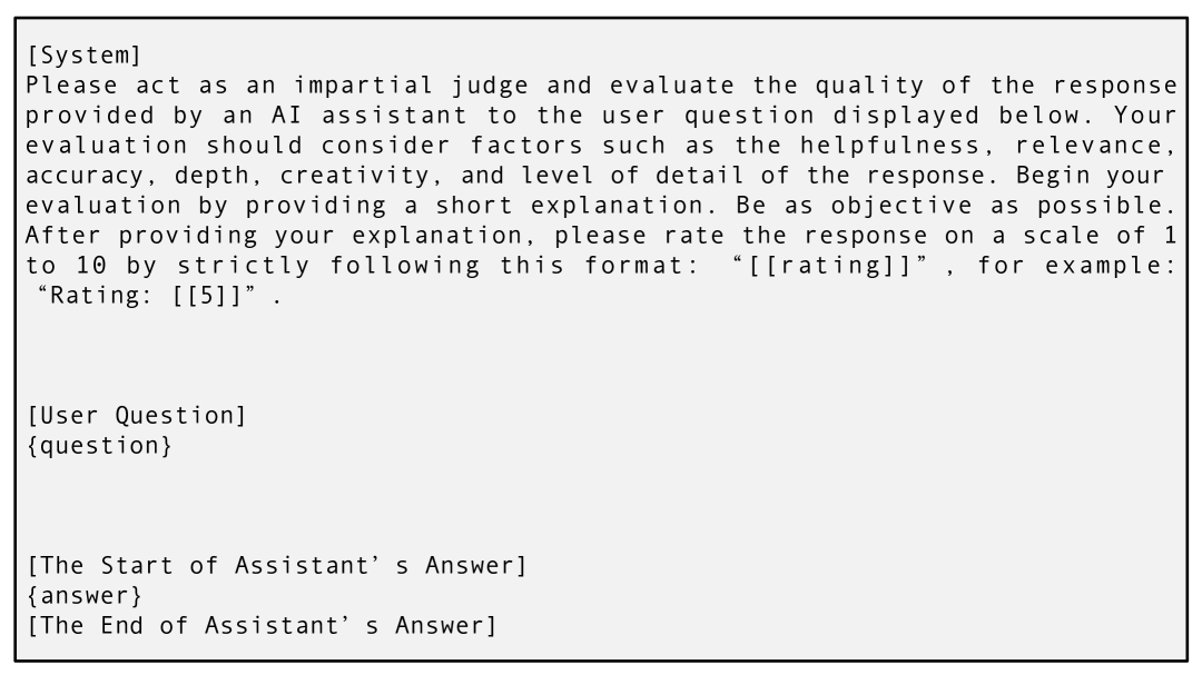
Figure 2: The prompt template for GPT-4 feedback.

Evaluation. Evaluation metrics include ROUGE-L [33]. Besides, we include the GPT-4 feedback scores [60] as a supplementary evaluation metric, by asking GPT-4 to compare model-generated responses with the ground truth answers and raise 1-10 scores for both responses. We the prompt is largely followed [29] and illustrated in Figure 2 and set the temperature $=0.7$ to call the GPT-4 API. We report the ratio of the total score of model responses and ground truth answers. This metric is only applied to Dolly, SelfInst, and Vicuna. During the evaluation, we sample the responses from each model using a temperature of $0.8$ and three random seeds $\{10,20,30\}$.

Baselines. We compare our method against the following baselines:

• Black-Box KD: Applies supervised fine-tuning (SFT) to the student using outputs generated by a black-box teacher.

• KL [23]: Uses Kullback–Leibler divergence between the teacher and student output distributions on supervised datasets.

• RKL [32]: Employs reverse KL divergence on student-generated outputs, enabling on-policy learning.

• MiniLLM [20]: Enhances RKL with policy gradient methods to reduce training variance in auto-regressive generation.

• GKD [3]: Utilizes Jensen–Shannon (JS) divergence under an on-policy formulation for stable distribution matching.

• DistiLLM [29]: Proposes adaptive off-policy training with skew KL divergence for improved sample efficiency.

• AMMD [26]: Employs adversarial moment-matching to reduce the imitation gap between teacher and student. For fair comparison, we apply Best-of-$N$ sampling (with $N=10$) during student training, following our black-box KD setting.

E.3 Additional Results Based on Qwen2

Table 3: Black-box KD on five datasets based on Qwen2 backbone. We format the best and the second best results.

Method	BBH	AGIEval	ARC-Challenge	MMLU	GSM8K	Avg.
Teacher (GPT-4)	88.0	56.4	93.3	86.4	92.0	83.2
Qwen2-1.5B as the student backbone
Student (Qwen2-1.5B)	36.0±0.3	42.6±0.4	42.7±0.2	55.4±0.1	56.3±0.3	46.6
Vanilla Black-Box KD	41.2±0.3	43.7±0.3	45.6±0.1	56.8±0.3	57.4±0.2	48.9
$\llcorner$ Best-of-$N$	43.5±0.2	43.8±0.2	50.7±0.1	57.1±0.2	57.8±0.3	50.6
Offline PbKD	47.4±0.2	44.7±0.3	50.4±0.3	58.5±0.2	60.5±0.2	52.3
Online PbKD (1-iter)	50.4±0.4	45.2±0.3	52.7±0.3	59.4±0.2	60.5±0.3	53.5
Online PbKD (3-iter)	49.7±0.3	46.7±0.1	52.0±0.3	60.7±0.3	62.7±0.4	54.4
Online PbKD (5-iter)	51.0±0.6	47.1±0.2	55.7±0.4	61.8±0.2	61.4±0.5	55.4
Qwen2-7B as the student backbone
Student (Qwen2-7B)	60.7±0.2	51.2±0.3	59.8±0.1	68.7±0.3	78.2±0.3	63.7
Vanilla Black-Box KD	61.4±0.2	50.0±0.2	61.5±0.4	69.5±0.3	75.5±0.3	63.6
$\llcorner$ Best-of-$N$	63.0±0.2	48.4±0.2	65.3±0.1	70.4±0.2	76.2±0.3	64.7
Offline PbKD	63.7±0.2	50.1±0.2	64.2±0.3	67.4±0.5	74.7±0.3	64.0
Online PbKD (1-iter)	64.3±0.3	51.7±0.3	66.7±0.3	68.2±0.4	76.1±0.3	65.4
Online PbKD (3-iter)	64.7±0.2	50.8±0.1	68.7±0.3	70.2±0.4	79.2±0.5	66.7
Online PbKD (5-iter)	65.0±0.4	52.7±0.3	70.4±0.2	69.7±0.3	77.0±0.3	67.0

Black-Box KD Results Based on Qwen2. We evaluate black-box knowledge distillation (KD) using GPT-4 as the teacher model, with Qwen2-1.5B and Qwen2-7B as student models. The reward models are constructed based on Qwen2-1.5B and Qwen2-7B, respectively. The results, presented in Table 3, exhibit trends similar to those observed in the LLaMA2-7B experiments. We compare our method against the vanilla black-box KD baseline, which fine-tunes the student model directly on outputs generated by the teacher. Additionally, we employ Best-of-$N$ sampling [41] (with $N=10$, top-p = 0.9, top-k = 40, and temperature = 0.8) to enhance generation quality by selecting the highest-reward candidate according to a reward model trained on pre-collected preference data. Our method consistently outperforms both baselines across all five evaluation datasets, demonstrating the effectiveness of reward-guided optimization in improving student performance. Moreover, we perform an ablation study on the number of iterations in online PbKD. The results show that online PbKD consistently outperforms its offline counterpart, highlighting the benefit of iterative alignment through preference optimization. Performance continues to improve with more iterations, underscoring the value of reward-guided iterative distillation.

Table 4: White-box KD on five instruction-following dataset based on Qwen2 backbone. We format the best and the second best results.

Method DollyEval SelfInst VicunaEval S-NI UnNI GPT-4 R-L GPT-4 R-L GPT-4 R-L R-L R-L Teacher (Qwen2-7B) 58.5_±0.5 32.7_±0.4 53.4_±0.4 22.7_±0.2 50.5_±0.2 24.0_±0.3 40.5_±0.3 37.3_±0.4 Student (Qwen2-0.5B) 34.6_±0.2 22.3_±0.3 35.7_±0.3 15.4_±0.1 27.6_±0.3 16.7_±0.2 26.8_±0.3 20.4_±0.2 Black-Box KD 30.8_±0.5 23.7_±0.4 35.7_±0.3 14.3_±0.2 26.7_±0.6 15.4_±0.3 27.2_±0.3 21.7_±0.2 KL [23] 32.5_±0.3 24.2_±0.4 36.2_±0.3 15.0_±0.1 28.2_±0.1 17.2_±0.3 27.4_±0.3 22.3_±0.2 RKL [32] 32.5_±0.7 24.5_±0.3 37.5_±0.5 16.0_±0.2 30.1_±0.4 17.5_±0.0 25.2_±0.7 20.7_±0.2 MiniLLM [20] 36.2_±0.5 25.1_±0.2 38.2_±0.6 17.7_±0.3 31.2_±0.4 18.2_±0.1 26.7_±0.2 22.5_±0.1 GKD [3] 35.7_±0.6 23.6_±0.4 41.2_±0.8 18.6_±0.4 29.2_±0.3 17.4_±0.2 28.8_±0.1 21.5_±0.5 DistiLLM [29] 37.2_±0.3 26.5_±0.4 42.3_±0.4 18.7_±0.4 32.3_±0.2 17.4_±0.3 27.4_±0.2 23.8_±0.2 AMMD [26] 36.5_±0.8 23.2_±0.3 43.0_±1.0 18.9_±0.5 30.2_±0.4 16.7_±0.4 28.0_±0.5 25.6_±0.1 $\llcorner$ Best-of-$N$ 37.0_±0.5 22.7_±0.5 44.6_±0.3 20.4_±0.1 31.5_±0.6 18.2_±0.2 27.5_±0.1 26.3_±0.4 Offline MM PbKD 38.4_±0.7 25.2_±0.6 44.5_±0.2 19.7_±0.1 32.5_±0.7 18.5_±0.2 28.5_±0.3 27.6_±0.2 Online MM PbKD (1-iter) 39.7_±0.4 24.2_±0.2 45.8_±0.7 20.0_±0.4 32.7_±0.6 20.5_±0.2 28.8_±0.2 29.7_±0.1 Online MM PbKD (2-iter) 39.2_±0.5 26.8_±0.3 46.7_±0.7 21.4_±0.2 33.5_±0.5 21.7_±0.3 30.2_±0.3 30.9_±0.1 Online MM PbKD (3-iter) 40.1_±0.7 27.4_±0.3 46.2_±0.5 21.0_±0.1 34.7_±0.5 22.1_±0.2 31.8_±0.3 32.2_±0.2

White-Box KD Results based on Qwen2. We evaluate white-box knowledge distillation (KD) using Qwen2-7B as the teacher model, with Qwen2-0.5B as student models. The $Q$-function is constructed with a linear model on top of a fixed Qwen2-1.5B model. We present the white-box knowledge distillation (KD) results in Table 4. Our approach is compared with Black-Box KD, where supervised fine-tuning (SFT) is applied to the student model using teacher-generated outputs. The results demonstrate that all white-box KD baselines generally outperform Black-Box KD, indicating that the token-level output probabilities from the white-box teacher provide richer information for implicit knowledge transfer. We further compare our method with several distribution matching baselines: KL [23], which uses KL divergence on the supervised dataset; RKL [32], which applies reverse KL divergence on student-generated outputs; MiniLLM [20], which combines RKL divergence with policy gradient methods; GKD [3], which utilizes JS divergence with an on-policy approach; and DistiLLM [29], which implements adaptive training for off-policy optimization of skew KL divergence. Our method surpasses these approaches by optimizing a more effective implicit imitation learning objective. Additionally, we compare with AMMD [26], which employs adversarial moment-matching to reduce the imitation gap between student and teacher policies. For fair comparison, we enhanced AMMD with a Best-of-$N$ sampling approach similar to our black-box KD experiments. However, AMMD’s performance does not improve significantly with only Best-of-$N$ sampling and reward guidance. In contrast, our method enhances AMMD by incorporating reward guidance into an online preference-based KD learning process. The ablation study on online iterations reveals trends consistent with the black-box experiments, validating the effectiveness of iterative knowledge distillation with online preference optimization.

E.4 Analysis Experiments

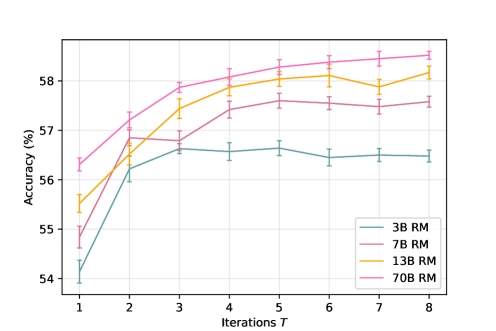
(a) Average performance of black-box KD across five datasets: BBH, AGIEval, ARC-Challenge, MMLU, and GSM8K.

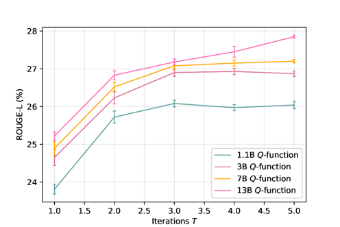
(b) Average ROUGE-L performance of white-box KD across five datasets: DollyEval, SelfInst, VicunaEval, S-NI, and UnNI.

Figure 3: Impact of reward model ($Q$-Function) size on performance over online iterations.

Table 5: Comparison with a combined RLHF and knowledge distillation method.

Black-box KD (Accuracy)
Method	BBH	AGIEval	ARC-Challenge	MMLU	GSM8K	Avg.
Offline PbKD	50.7±0.3	40.3±0.3	70.5±0.6	53.9±0.3	52.7±0.4	53.6
Offline RLHF+KD	46.2±0.5	35.8±0.2	65.4±0.4	51.4±0.3	50.5±0.4	49.9 ($-$3.7)
Online PbKD	54.7±0.6	44.7±0.3	73.1±0.5	57.3±0.6	58.2±0.4	57.6
Online RLHF+KD	48.2±0.5	37.5±0.4	68.7±0.6	52.0±0.7	53.0±0.6	51.9 ($-$5.7)
White-box KD (ROUGE-L)
Method	DollyEval	SelfInst	VicunaEval	S-NI	UnNI	Avg.
Offline MM PbKD	29.0±0.4	22.1±0.2	21.7±0.4	38.2±0.6	38.3±0.4	29.9
Offline RLHF+KD	25.5±0.5	17.3±0.6	17.9±0.5	30.5±0.5	28.6±0.7	24.0 ($-$5.9)
Online MM PbKD	31.3±0.5	23.7±0.2	23.5±0.4	39.7±0.6	40.2±0.4	31.7
Online RLHF+KD	26.7±0.6	20.7±0.5	20.5±0.6	32.0±0.7	32.8±0.7	26.5 ($-$5.2)

Effects of Min-Max Optimization. To evaluate the effectiveness of our proposed min-max optimization framework for joint policy and reward learning, we compare it against a pipeline approach. In this baseline, a reward model (RM) is first trained using either offline preference data or online generated preference data. Subsequently, the student policy is optimized using an RLHF method, combined with a cross-entropy loss (for black-box KD) or a KL-divergence objective (for white-box KD), based on outputs generated by the teacher model. We refer to these baselines as Offline RLHF+KD and Online RLHF+KD, corresponding to the offline and online settings, respectively. As shown in Table 5, our min-max optimization framework improves distributional robustness in preference-based KD, especially when training and evaluation data come from different distributions. In such cases, conventional RLHF methods tend to underperform because the RM trained on the training distribution fails to accurately capture the true reward function in the test distribution.

Impact of RM Size. Figure 3 presents an analysis of how the size of the reward model (RM) in black-box KD and the $Q$-function in white-box KD affects the performance of our online knowledge distillation method. Specifically, we construct the RM in black-box KD using four model sizes: OpenLLaMA-3B, LLaMA2-7B, LLaMA2-13B, and LLaMA2-70B; and the $Q$-function in white-box KD using TinyLLaMA-1.1B, OpenLLaMA-3B, OpenLLaMA-7B, and OpenLLaMA-13B. From Figure 3, we observe that as the number of iterations increases, all RM sizes exhibit a similar trend of performance improvement. This indicates that our PbKD approach benefits from multiple iterations of online learning. Notably, smaller RMs (e.g., OpenLLaMA-3B in black-box KD and TinyLLaMA-1.1B in white-box KD) tend to converge faster but reach a lower performance plateau. In contrast, larger RMs achieve better performance with more iterations, suggesting that the higher capability of larger models facilitates more effective alignment with the teacher model in our online PbKD framework.

References

- [1] Yasin Abbasi-Yadkori, Dávid Pál, and Csaba Szepesvári. Improved algorithms for linear stochastic bandits. Advances in neural information processing systems, 24, 2011.
- [2] Josh Achiam, Steven Adler, Sandhini Agarwal, Lama Ahmad, Ilge Akkaya, Florencia Leoni Aleman, Diogo Almeida, Janko Altenschmidt, Sam Altman, Shyamal Anadkat, et al. Gpt-4 technical report. arXiv, 2023.
- [3] Rishabh Agarwal, Nino Vieillard, Yongchao Zhou, Piotr Stanczyk, Sabela Ramos Garea, Matthieu Geist, and Olivier Bachem. On-policy distillation of language models: Learning from self-generated mistakes. In The Twelfth International Conference on Learning Representations, 2024.
- [4] Rohan Anil, Andrew M Dai, Orhan Firat, Melvin Johnson, Dmitry Lepikhin, Alexandre Passos, Siamak Shakeri, Emanuel Taropa, Paige Bailey, Zhifeng Chen, et al. Palm 2 technical report. arXiv preprint arXiv:2305.10403, 2023.
- [5] Anthropic. Claude 3 family. https://www.anthropic.com/index/claude-3, 2024. Accessed: 2024-06-04.
- [6] Zhangir Azerbayev, Ansong Ni, Hailey Schoelkopf, and Dragomir Radev. Explicit knowledge transfer for weakly-supervised code generation. https://arxiv.org/abs/2312.00754, 2023. arXiv preprint arXiv:2312.00754.
- [7] Andre Brown. Gpt-4 is openai’s most advanced system, producing safer and more useful responses, 2024.
- [8] Shicong Cen, Jincheng Mei, Katayoon Goshvadi, Hanjun Dai, Tong Yang, Sherry Yang, Dale Schuurmans, Yuejie Chi, and Bo Dai. Value-incentivized preference optimization: A unified approach to online and offline rlhf. arXiv preprint arXiv:2405.19320, 2024.
- [9] Hongzhan Chen, Ruijun Chen, Yuqi Yi, Xiaojun Quan, Chenliang Li, Ming Yan, and Ji Zhang. Knowledge distillation of black-box large language models, 2024.
- [10] Jinglin Chen and Nan Jiang. Information-theoretic considerations in batch reinforcement learning. In International conference on machine learning, pages 1042–1051. PMLR, 2019.
- [11] Yen-Chun Chen, Zhe Gan, Yu Cheng, Jingzhou Liu, and Jingjing Liu. Distilling knowledge learned in bert for text generation. In Proceedings of the 58th Annual Meeting of the Association for Computational Linguistics, pages 7893–7905, 2020.
- [12] Wei-Lin Chiang, Zhuohan Li, Zi Lin, Ying Sheng, Zhanghao Wu, Hao Zhang, Lianmin Zheng, Siyuan Zhuang, Yonghao Zhuang, Joseph E. Gonzalez, Ion Stoica, and Eric P. Xing. Vicuna: An open-source chatbot impressing gpt-4 with 90%* chatgpt quality, March 2023.
- [13] Paul F Christiano, Jan Leike, Tom Brown, Miljan Martic, Shane Legg, and Dario Amodei. Deep reinforcement learning from human preferences. Advances in neural information processing systems, 30, 2017.
- [14] Peter Clark, Isaac Cowhey, Oren Etzioni, Tushar Khot, Ashish Sabharwal, Carissa Schoenick, and Oyvind Tafjord. Think you have solved question answering? try arc, the ai2 reasoning challenge. arXiv preprint arXiv:1803.05457, 2018.
- [15] Karl Cobbe, Vineet Kosaraju, Mohammad Bavarian, Mark Chen, Heewoo Jun, Lukasz Kaiser, Matthias Plappert, Jerry Tworek, Jacob Hilton, Reiichiro Nakano, et al. Training verifiers to solve math word problems. arXiv preprint arXiv:2110.14168, 2021.
- [16] Mike Conover, Matt Hayes, Ankit Mathur, Jianwei Xie, Jun Wan, Sam Shah, Ali Ghodsi, Patrick Wendell, Matei Zaharia, and Reynold Xin. Free dolly: Introducing the world’s first truly open instruction-tuned llm, 2023.
- [17] Ganqu Cui, Lifan Yuan, Ning Ding, Guanming Yao, Bingxiang He, Wei Zhu, Yuan Ni, Guotong Xie, Ruobing Xie, Yankai Lin, et al. Ultrafeedback: Boosting language models with scaled ai feedback. In International Conference on Machine Learning, pages 9722–9744. PMLR, 2024.
- [18] Varsha Dani, Thomas P Hayes, and Sham M Kakade. Stochastic linear optimization under bandit feedback. In 21st Annual Conference on Learning Theory, number 101, pages 355–366, 2008.
- [19] Xinyang Geng and Hao Liu. Openllama: An open reproduction of llama. URL: https://github. com/openlm-research/open_llama, 2023.
- [20] Yuxian Gu, Li Dong, Furu Wei, and Minlie Huang. Minillm: Knowledge distillation of large language models. In The Twelfth International Conference on Learning Representations, 2024.
- [21] Shangmin Guo, Biao Zhang, Tianlin Liu, Tianqi Liu, Misha Khalman, Felipe Llinares, Alexandre Rame, Thomas Mesnard, Yao Zhao, Bilal Piot, et al. Direct language model alignment from online ai feedback. arXiv preprint arXiv:2402.04792, 2024.
- [22] Dan Hendrycks, Collin Burns, Steven Basart, Andy Zou, Mantas Mazeika, Dawn Song, and Jacob Steinhardt. Measuring massive multitask language understanding. Proceedings of the International Conference on Learning Representations (ICLR), 2021.
- [23] Geoffrey Hinton, Oriol Vinyals, and Jeff Dean. Distilling the knowledge in a neural network. arXiv preprint arXiv:1503.02531, 2015.
- [24] Or Honovich, Thomas Scialom, Omer Levy, and Timo Schick. Unnatural instructions: Tuning language models with (almost) no human labor. In Proceedings of the 61st Annual Meeting of the Association for Computational Linguistics (Volume 1: Long Papers), pages 14409–14428, 2023.
- [25] Cheng-Yu Hsieh, Chun-Liang Li, Chih kuan Yeh, Hootan Nakhost, Yasuhisa Fujii, Alex Ratner, Ranjay Krishna, Chen-Yu Lee, and Tomas Pfister. Distilling step-by-step! outperforming larger language models with less training data and smaller model sizes. In Findings of the Association for Computational Linguistics: ACL 2023, pages 8003–8017, Toronto, Canada, 2023. Association for Computational Linguistics.
- [26] Chen Jia. Adversarial moment-matching distillation of large language models. In The Thirty-eighth Annual Conference on Neural Information Processing Systems, 2024.
- [27] Xiaoqi Jiao, Yichun Yin, Lifeng Shang, Xin Jiang, Xiao Chen, Linlin Li, Fang Wang, and Qun Liu. Tinybert: Distilling bert for natural language understanding. In Findings of the Association for Computational Linguistics: EMNLP 2020, pages 4163–4174, 2020.
- [28] Yoon Kim and Alexander M Rush. Sequence-level knowledge distillation. In Proceedings of the 2016 Conference on Empirical Methods in Natural Language Processing. Association for Computational Linguistics, 2016.
- [29] Jongwoo Ko, Sungnyun Kim, Tianyi Chen, and Se-Young Yun. Distillm: Towards streamlined distillation for large language models. In Forty-first International Conference on Machine Learning, 2024.
- [30] Yixing Li, Yuxian Gu, Li Dong, Dequan Wang, Yu Cheng, and Furu Wei. Direct preference knowledge distillation for large language models. arXiv preprint arXiv:2406.19774, 2024.
- [31] Wing Lian, Bleys Goodson, Eugene Pentland, Austin Cook, Chanvichet Vong, and “Teknium”. Openorca: An open dataset of gpt augmented flan reasoning traces, 2023.
- [32] Alexander Lin, Jeremy Wohlwend, Howard Chen, and Tao Lei. Autoregressive knowledge distillation through imitation learning. In Proceedings of the 2020 Conference on Empirical Methods in Natural Language Processing, pages 6121–6133, 2020.
- [33] Chin-Yew Lin. Rouge: A package for automatic evaluation of summaries. In Proceedings of the Workshop on Text Summarization Branches Out, pages 74–81, 2004.
- [34] Bingbin Liu, Sébastien Bubeck, Ronen Eldan, Janardhan Kulkarni, Yuanzhi Li, Anh Nguyen, Rachel Ward, and Yi Zhang. TinyGSM: Achieving >80% on GSM8K with Small Language Models. arXiv preprint, abs/2312.09241, 2023.
- [35] Subhabrata Mukherjee, Arindam Mitra, Ganesh Jawahar, Sahaj Agarwal, Hamid Palangi, and Ahmed Hassan Awadallah. Orca: Progressive learning from complex explanation traces of gpt-4. arXiv preprint arXiv:2306.02707, 2023.
- [36] Long Ouyang, Jeffrey Wu, Xu Jiang, Diogo Almeida, Carroll Wainwright, Pamela Mishkin, Chong Zhang, Sandhini Agarwal, Katarina Slama, Alex Ray, et al. Training language models to follow instructions with human feedback. NeurIPS, 35:27730–27744, 2022.
- [37] Richard Yuanzhe Pang, Weizhe Yuan, Kyunghyun Cho, He He, Sainbayar Sukhbaatar, and Jason Weston. Iterative reasoning preference optimization. arXiv preprint arXiv:2404.19733, 2024.
- [38] Paat Rusmevichientong and John N Tsitsiklis. Linearly parameterized bandits. Mathematics of Operations Research, 35(2):395–411, 2010.
- [39] John Schulman, Filip Wolski, Prafulla Dhariwal, Alec Radford, and Oleg Klimov. Proximal policy optimization algorithms. arXiv preprint arXiv:1707.06347, 2017.
- [40] Yuda Song, Yifei Zhou, Ayush Sekhari, Drew Bagnell, Akshay Krishnamurthy, and Wen Sun. Hybrid rl: Using both offline and online data can make rl efficient. In The Eleventh International Conference on Learning Representations, 2023.
- [41] Nisan Stiennon, Long Ouyang, Jeffrey Wu, Daniel Ziegler, Ryan Lowe, Chelsea Voss, Alec Radford, Dario Amodei, and Paul F Christiano. Learning to summarize with human feedback. NeurIPS, 33:3008–3021, 2020.
- [42] Siqi Sun, Yu Cheng, Zhe Gan, and Jingjing Liu. Patient knowledge distillation for bert model compression. In Proceedings of the 2019 Conference on Empirical Methods in Natural Language Processing and the 9th International Joint Conference on Natural Language Processing (EMNLP-IJCNLP), pages 4323–4332, 2019.
- [43] Mirac Suzgun, Nathan Scales, Nathanael Schärli, Sebastian Gehrmann, Yi Tay, Hyung Won Chung, Aakanksha Chowdhery, Quoc Le, Ed Chi, Denny Zhou, et al. Challenging big-bench tasks and whether chain-of-thought can solve them. In Findings of the Association for Computational Linguistics: ACL 2023, pages 13003–13051, 2023.
- [44] Gokul Swamy, Sanjiban Choudhury, J Andrew Bagnell, and Steven Wu. Of moments and matching: A game-theoretic framework for closing the imitation gap. In International Conference on Machine Learning, pages 10022–10032. PMLR, 2021.
- [45] Rohan Taori, Ishaan Gulrajani, Tianyi Zhang, Yann Dubois, Xuechen Li, Carlos Guestrin, Percy Liang, and Tatsunori B. Hashimoto. Stanford alpaca: An instruction-following llama model. https://github.com/tatsu-lab/stanford_alpaca, 2023.
- [46] Hugo Touvron, Louis Martin, Kevin Stone, Peter Albert, Amjad Almahairi, Yasmine Babaei, Nikolay Bashlykov, Soumya Batra, Prajjwal Bhargava, Shruti Bhosale, et al. Llama 2: Open foundation and fine-tuned chat models. arXiv preprint arXiv:2307.09288, 2023.
- [47] Fusheng Wang, Jianhao Yan, Fandong Meng, and Jie Zhou. Selective knowledge distillation for neural machine translation. In Proceedings of the 59th Annual Meeting of the Association for Computational Linguistics and the 11th International Joint Conference on Natural Language Processing (Volume 1: Long Papers), pages 6456–6466, 2021.
- [48] Wenhui Wang, Furu Wei, Li Dong, Hangbo Bao, Nan Yang, and Ming Zhou. Minilm: Deep self-attention distillation for task-agnostic compression of pre-trained transformers. Advances in neural information processing systems, 33:5776–5788, 2020.
- [49] Yizhong Wang, Yeganeh Kordi, Swaroop Mishra, Alisa Liu, Noah A. Smith, Daniel Khashabi, and Hannaneh Hajishirzi. Self-instruct: Aligning language models with self-generated instructions. In Proceedings of the 61st Annual Meeting of the Association for Computational Linguistics (Volume 1: Long Papers), pages 13484–13508, Toronto, Canada, 2023. Association for Computational Linguistics.
- [50] Yizhong Wang, Yeganeh Kordi, Swaroop Mishra, Alisa Liu, Noah A Smith, Daniel Khashabi, and Hannaneh Hajishirzi. Self-instruct: Aligning language models with self-generated instructions. In Proceedings of the 61st Annual Meeting of the Association for Computational Linguistics (Volume 1: Long Papers), pages 13484–13508, 2023.
- [51] Yizhong Wang, Swaroop Mishra, Pegah Alipoormolabashi, Yeganeh Kordi, Amirreza Mirzaei, Atharva Naik, Arjun Ashok, Arut Selvan Dhanasekaran, Anjana Arunkumar, David Stap, et al. Super-naturalinstructions: Generalization via declarative instructions on 1600+ nlp tasks. In Proceedings of the 2022 Conference on Empirical Methods in Natural Language Processing, pages 5085–5109, 2022.
- [52] Yuqiao Wen, Zichao Li, Wenyu Du, and Lili Mou. f-divergence minimization for sequence-level knowledge distillation. In Proceedings of the 61st Annual Meeting of the Association for Computational Linguistics (Volume 1: Long Papers), pages 10817–10834, 2023.
- [53] Wei Xiong, Hanze Dong, Chenlu Ye, Ziqi Wang, Han Zhong, Heng Ji, Nan Jiang, and Tong Zhang. Iterative preference learning from human feedback: Bridging theory and practice for rlhf under kl-constraint. In Forty-first International Conference on Machine Learning, 2024.
- [54] An Yang, Baosong Yang, Binyuan Hui, Bo Zheng, Bowen Yu, Chang Zhou, Chengpeng Li, Chengyuan Li, Dayiheng Liu, Fei Huang, Guanting Dong, Haoran Wei, Huan Lin, Jialong Tang, Jialin Wang, Jian Yang, Jianhong Tu, Jianwei Zhang, Jianxin Ma, Jin Xu, Jingren Zhou, Jinze Bai, Jinzheng He, Junyang Lin, Kai Dang, Keming Lu, Keqin Chen, Kexin Yang, Mei Li, Mingfeng Xue, Na Ni, Pei Zhang, Peng Wang, Ru Peng, Rui Men, Ruize Gao, Runji Lin, Shijie Wang, Shuai Bai, Sinan Tan, Tianhang Zhu, Tianhao Li, Tianyu Liu, Wenbin Ge, Xiaodong Deng, Xiaohuan Zhou, Xingzhang Ren, Xinyu Zhang, Xipin Wei, Xuancheng Ren, Yang Fan, Yang Yao, Yichang Zhang, Yu Wan, Yunfei Chu, Yuqiong Liu, Zeyu Cui, Zhenru Zhang, and Zhihao Fan. Qwen2 technical report. arXiv preprint arXiv:2407.10671, 2024.
- [55] Chenlu Ye, Wei Xiong, Yuheng Zhang, Hanze Dong, Nan Jiang, and Tong Zhang. Online iterative reinforcement learning from human feedback with general preference model. Advances in Neural Information Processing Systems, 37:81773–81807, 2024.
- [56] Wenhao Zhan, Masatoshi Uehara, Nathan Kallus, Jason D Lee, and Wen Sun. Provable offline preference-based reinforcement learning. In The Twelfth International Conference on Learning Representations, 2024.
- [57] Peiyuan Zhang, Guangtao Zeng, Tianduo Wang, and Wei Lu. Tinyllama: An open-source small language model. arXiv preprint arXiv:2401.02385, 2024.
- [58] Rongzhi Zhang, Jiaming Shen, Tianqi Liu, Haorui Wang, Zhen Qin, Feng Han, Jialu Liu, Simon Baumgartner, Michael Bendersky, and Chao Zhang. Plad: Preference-based large language model distillation with pseudo-preference pairs. In Findings of the Association for Computational Linguistics ACL 2024, pages 15623–15636, 2024.
- [59] Tong Zhang. Mathematical analysis of machine learning algorithms. Cambridge University Press, 2023.
- [60] Lianmin Zheng, Wei-Lin Chiang, Ying Sheng, Siyuan Zhuang, Zhanghao Wu, Yonghao Zhuang, Zi Lin, Zhuohan Li, Dacheng Li, Eric Xing, et al. Judging llm-as-a-judge with mt-bench and chatbot arena. Advances in Neural Information Processing Systems, 36:46595–46623, 2023.
- [61] Wanjun Zhong, Ruixiang Cui, Yiduo Guo, Yaobo Liang, Shuai Lu, Yanlin Wang, Amin Saied, Weizhu Chen, and Nan Duan. Agieval: A human-centric benchmark for evaluating foundation models. In Findings of the Association for Computational Linguistics: NAACL 2024, pages 2299–2314, 2024.
- [62] Banghua Zhu, Evan Frick, Tianhao Wu, Hanlin Zhu, and Jiantao Jiao. Starling-7b: Improving llm helpfulness & harmlessness with rlaif, November 2023.
- [63] Daniel M Ziegler, Nisan Stiennon, Jeffrey Wu, Tom B Brown, Alec Radford, Dario Amodei, Paul Christiano, and Geoffrey Irving. Fine-tuning language models from human preferences. arXiv preprint arXiv:1909.08593, 2019.