Condensate Fraction Scaling and Specific Heat Anomaly around Berezinskii-Kosterlitz-Thouless Transition of Superconductivity and Superfluidity
Abstract
Characterizing the superconducting and superfluid transitions in two-dimensional (2D) many-body systems is of broad interest and remains a fundamental issue. In this study, we establish the condensate fraction as a highly effective tool to achieve that and accordingly propose efficient schemes for accurately determining the transitions, via numerically exact quantum Monte Carlo simulations. Using the 2D attractive Fermi-Hubbard model as a testbed, we access unprecedented system sizes (up to 4096 lattice sites) and perform a comprehensive analysis for the temperature dependence and finite-size scaling of condensate fraction across the Berezinskii-Kosterlitz-Thouless (BKT) transition. We demonstrate that this quantity exhibits algebraic scaling below the transition and exponential scaling above it, with significantly smaller finite-size effect comparing to the extensively studied on-site pairing correlator. This greatly improves the determination of BKT transition with moderate system sizes. We also extract the finite-size BKT transition temperature from condensate fraction, and confirm its logarithmic correction on system size. Furthermore, we find that the specific heat displays an anomaly, showing a peak at a temperature slightly above BKT transition. Our findings should be generally applicable to 2D fermionic and bosonic systems hosting superconductivity or superfluidity.
Berezinskii-Kosterlitz-Thouless (BKT) transition [1, 2, 3] is one of the most intriguing property of two-dimensional (2D) systems with U(1) continuous symmetry and short-range interactions. The transition towards the low-temperature phase is typically characterized [4] by the formation of bounded vortex-antivortex pairs and a quasi-long-range order with algebraically decaying correlation function with distance. The most representative examples are 2D superconductivity and superfluidity, for which the theory also predicts a universal jump of the superfluid density [5] at the BKT transition. These key signatures of BKT physics was experimentally verified in liquid [6, 7] and superconducting films [8, 9, 10] soon after the celebrated BKT theory, and more recently in 2D interacting Bose gas [11, 12, 13] and Fermi gas [14, 15]. The rapid progress in ultracold atom systems has enabled the detailed studies of the BKT transition, and many more experiments with growing precision continue to reveal its other rich properties, such as the phase fluctuations [16], transport and excitation signatures [17, 18, 19, 20].
Theoretically, the thorough characterization and precise determination of the BKT transition primarily rely on numerically unbiased calculations [21, 22, 23, 24, 25, 26, 27, 28, 29, 30, 31, 32, 33, 34, 35, 36, 37, 38, 39, 40, 41, 42, 43]. Regarding superconductivity and superfluidity, the 2D attractive Hubbard model serves as the minimal model that captures the BKT physics, as investigated by auxiliary-field quantum Monte Carlo (AFQMC) simulations [33, 34, 35, 36, 37, 38, 39, 40, 41]. These studies typically estimated the BKT transition temperature through finite-size analyses of the on-site spin-singlet pairing correlation or the superfluid density [44, *Scalapino1993]. However, both quantities exhibit pronounced finite-size effects, which compromise the reliability of standard scaling approaches. In addition, extracting superfluid density from the dynamical current-current correlation function is computationally demanding and usually yields notably noisy results [36, 38, 39]. All of these studies have been constrained to lattice sizes of up to 400 sites, which are likely insufficient to capture the logarithmic finite-size corrections characteristic of BKT transition [25, 30, 23]. These limitations hinder high-precision determination of BKT transition temperature, even when using numerically exact AFQMC simulations.
Alternatively, condensate fraction is also a fundamental quantity to characterize the superconducting and superfluid states [46, 47, 48], defined as the proportion of Bose-condensed bosons or fermion pairs. It was experimentally measured in liquid [49] system and ultracold Fermi gas [50, 51, 52] in three dimensions, and found to behave similarly as the pairing order parameter with its onset identifying the superfluid phase transtion. In these systems, this quantity has also been theoretically computed by mean-field theories [53, 54, 48, 55] as well as many-body numerical methods [47, 56, 57, 58, 59] at both ground state and finite temperatures. In contrast, it is much less studied for 2D superconductivity and superfluidity in many-body systems especially at finite temperatures. Until now, the theoretical and numerical studies of this quantity mainly concentrate on the ground-state results of 2D interacting Fermi gas [60, 61, 62]. Then the natural questiones arise as the behaviors of this quantity around the BKT transition and whether it could be used to probe the transition.
We address the questions by systematically exploring the temperature and size dependences of condensate fraction across the BKT transition in the 2D attractive Hubbard model with large-scale and numerically unbiased AFQMC algorithm. Our calculations reach lattice sizes of up to sites, an order of magnitude larger than that in previous studies [33, 34, 35, 36, 37, 38, 39, 40, 41]. This enables us to perform a finite-size scaling analysis of BKT physics in correlated fermion systems with unprecedented high quality. Our numerical results reveal the algebraic (exponential) scaling of condensate fraction in the superfluid (normal) phase, and establish it as a much more effective probe for characterizing the BKT transition, compared to the long-studied on-site pairing correlator. Then we have computed accurate BKT transition temperature based on the scaling behaviors of condensate fraction. A clear evidence of specific heat anomaly above the BKT transition is also identified in our calculations.
We study the 2D attractive Fermi-Hubbard model on square lattice with the Hamiltonian as
| (1) |
with as the density operator and ( or ) denoting spin. We only consider the nearest-neighbor hopping with the energy dispersion , where are the momentum defined in units of with linear system size . The fermion filling is with and as the number of lattice sites and fermions. We set as the energy unit, and focus on attractive interaction with hole doping . It is well-known that this model has a superconducting ground state [63, 64, 65] and exhibits BKT transition at finite temperatures [33, 34, 35, 36]. We employ state-of-art AFQMC algorithm [66, 67, 68, 69, 70, 71, 72] with most recent developments [73] to study the BKT physics in this model. Our simulations cover a large range of system sizes, from to .
We mainly focus on the condensate fraction and on-site pairing correlator, which both characterize the fermion pairing. The first is initially defined from the macroscopic eigenvalue of the two-body density matrix, expressed as , in asymptotic limit [46, 47]. Regarding attractive interaction, we only need to focus on the dominant component of , i.e., the pairing matrix in momentum space [61, 42, 43] as , with as the -space spin-singlet pairing operator. Then condensate fraction can be calculated as , with as the leading eigenvalue of matrix. The corresponding eigenvector of contains the pairing structure information in space [73]. On the other hand, the pairing correlation is defined as with on-site pairing operator . The corresponding pairing correlator reads , which has been studied for attractive fermions over decades [33, 34, 35, 36, 37, 38, 39, 40, 41]. For 2D superfluid phase, decays algebraically as with and at BKT transition [1, 2, 3], leading to the scaling behavior of in large limit [73]. In contrast, they simply decay exponentially in the normal phase.
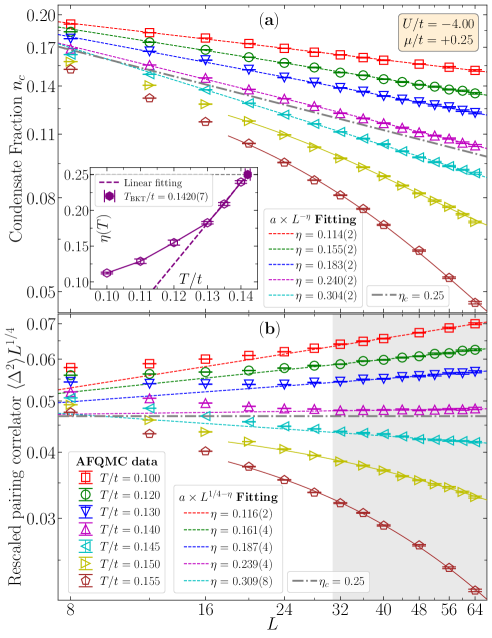
As the main results of this work, Fig. 1 summarizes finite-size scaling behaviors of condensate fraction and on-site pairing correlator for . Upon cooling, monotonically grows as evolving from the normal phase to the superfluid phase [73]. Then the log-log plot and fittings for the numerical results in Fig. 1(a) clearly reveal that also has algebraic () and exponential () scalings versus in the low and high temperature regimes, respectively. As a comparison, Fig. 1(b) plots versus , and the results with confirm the size-scaling behaviors of from BKT theory. As it is straightforward, the horizontal line (gray, dash-dot) denoting in Fig. 1(b) determines the BKT transition temperature in the range of , which perfectly matches to that from results in Fig. 1(a). Moreover, the fittings of these two quantities presents well consistent exponents within statistical uncertainty, indicating exactly the same size-scaling behavior of them (in large limit). Note that for , the algebraic scaling should gradually crossover to exponential decay at larger system sizes even beyond the reach of our AFQMC calculations. These results explicitly illustrate vanishing and approaching the thermodynamic limit (TDL) at finite temperatures, and confirms the quasi-condensate and quasi-long-range order state in the 2D superfluid phase. Furthermore, as shown in the inset of Fig. 1(a), the exponent exhibits linear scaling with temperature near the transition point from below, , yielding the transition temperature at TDL.
It is noteworthy that Fig. 1 reveals a prominent discrepancy between and . The latter shows a pronounced finite-size effect, with results for clearly deviating from the correct scaling behavior observed in larger systems (especially for ), as shown in Fig. 1(b). If the numerical simulations are restricted to , as in previous studies [33, 34, 36, 37, 38, 39, 40, 41], one would obtain the BKT transition temperature in the range , consistent with that reported in Ref. 41, but with an error exceeding relative to the correct value. Nevertheless, condensate fraction shown in Fig. 1(a) exhibits much better size-scaling behavior around BKT transition. Results for are sufficient to accurately determine the BKT transition temperature, with a small interval of , pinning it down to the quantitatively correct range. This difference can be attributed to the distinct underlying physics of these two quantities. Formally, includes a subleading correction [73], in addition to the leading term . Physically, while only accounts for on-site pairing, the pairing matrix originates from -space pairing, meaning that encompasses contributions from Cooper pairs of all possible sizes. For weak to intermediate attractive interactions, nonlocal fermion pairing is non-negligible, as evidenced by AFQMC results of real-space pair wave function [73], and has also been observed in a recent optical lattice experiment [74]. The contribution from local Cooper pairs to the overall pairing can fluctuate significantly with system size. As a result, the quantity fails to capture the full pairing structure of the system and is subject to strong finite-size effects.
We have obtained similar results as above for diffrent fermion fillings and interaction strengths [73]. Our numerical results show that the finite-size effect of the on-site pairing correlator (as deviation from the correct scaling in small sizes) gets more severe for lower filling and weaker interaction. This can be understood from the fact that the the nonlocal pairing becomes more significant in these systems. Instead, such effect is almost absent in condensate fraction with its numerical results always exhibiting nice size-scaling behavior for as those shown in Fig. 1(a). This implies that it is much more challenging to accurately determine BKT transition in 2D interacting Fermi gas [43] via finite-size analysis of results than that with . All these results suggest that condensate fraction is a more appropriate quantity for characterizing the fermion pairing and determining BKT transition for attracive fermions. Our calculations of superfluid density [44, 45] up to also conform with the BKT transition temperature obtained from the finite-size scaling of the condensate fraction [73].
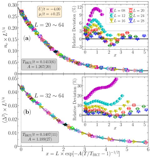
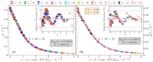
With the above bounded range, the precise can be further extracted from standard finite-size scaling. The most commonly used method is via the data collapse of the pairing correlator [33, 34, 36, 37, 38, 39, 40, 41]. It is based on the scaling relation with slightly above the transition as [36, 30, 41]. The fitting process determines , and , which then make the plot of collapse into a universal curve of . Similarly, condensate fraction should also satisfy the above scaling relation since it has the same scaling behavior as . We then perform data collapse for both and with fixed for the results presented in Fig. 1. Considering the finite-size effect in , we use numerical results of for and for in the fitting, for which we adopt polynomials for around and apply the least-squares criterion. The data collapse results are plotted in Fig. 2. Consistent results of and are obtained respectively from and , which agree with the bounded range obtained in Fig. 1. The insets of Fig. 2, showing relative deviations from of results, reveal the more severe finite-size effect in than that of . Specifically, the maximum deviation for is in , whereas it is for . Further including data in the fitting for indeed leads to a lower out of the bounded range.

An alternative way to compute BKT transition temperature is to first obtain the finite-size result and then extrapolate it to TDL. They satisfy a logarithmic correction relation as [23, 24, 25, 30, 31, 32]. This method has been applied in numerical simulations of Ising model [31], XY model [25, 30], and dipolar boson system [24].
The change from algebraic to exponential scaling behaviors of condensate fraction across the BKT transition naturally gives rise to an inflection point in its temperature dependence, . Here we identify this inflection point as . As illustrated in Fig. 3(a) for two representative sets of AFQMC data, we first perform fitting for and then determine the inflection point as the peak location of using the fitting curve. The uncertainty of is estimated via bootstrapping [75]. The consistent results of from the fitting and the numerical differentiation using total-variation regularization [76, 77] in the inset of Fig. 3(a) validates our procedure of computing . We repeat this procedure for , and perform the scaling for using the above logarithmic relation. Due to limited precision, we fix the parameter in the fitting, as in previous studies [24, 31, 32]. The results for [] and [] are plotted in Fig. 3(b). TDL transition temperatures of and are reached for these two cases, respectively, with and at the transition [73]. These numbers are consistent with those obtained from the scaling and the data collapse [see Figs. 1(a) and 2(a) for , and Ref. 73 for ]. The inset of Fig. 3(b) shows the fitting for , which yields noticeably noisier estimates of compared to the fixed case, but remains consistent within the uncertainty. We have also tried polynomial fits in for , which all produce higher than the corresponding bounded range. It thereby supports the validity of the logarithmic correction form instead.
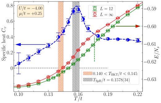
Highly accurate BKT transition temperature can have broad applications in uncovering the underlying physics of 2D correlated systems. One example is the behavior of thermodynamics near the BKT transition. Among these, specific heat is a particularly important and widely used observable for detecting phase transitions [52]. However, previous studies showed that the specific heat exhibits a peak at in 2D [7] and in 2D XY model [26, 27, 28, 29, 30]. Our results also confirm the existence of such anomaly in the 2D attractive Hubbard model. We compute the specific heat using with as the total energy. Through fitting , the energy derivative is evaluated analytically from the fitting curve. Results of (, and from extrapolations) and (at TDL) are presented in Fig. 4 for . The specific heat obtained consistently from both energy fitting and numerical differentiation [76, 77] exhibits a pronounced peak at . Similar behavior is observed in calculations at other fixed values of , with comparable ratios of and a notable trend of decreasing peak height in as the filling is reduced [73]. This specific heat anomaly can be attributed to the maximal rate of vortex formation which costs energy, as revealed in 2D XY model [26, 27, 28], and is therefore not directly related to the BKT transition. Nevertheless, it may serve as a precursor signature of the system approaching BKT transition in future optical lattice experiments for the 2D attracive Hubbard model, for which the BKT physics remains inaccessible [74].
We have uncovered the scaling behaviors of condensate fraction and developed schemes based on this quantity to estimate BKT transition temperature in the 2D attractive Fermi-Hubbard model. These behaviors and schemes can be readily extended to other 2D correlated fermion systems exhibiting superconductivity or superfluidity, including those with spin-orbit coupling (SOC) [62, 78, 75], interacting Fermi gases [61, 43]. In the presence of SOC, condensate fraction can be similarly computed from a modified pairing matrix , which incorporates both spin-singlet and spin-triplet pairing [75, 79]. Accordingly, the pairing correlators suffer the same issues as shown in Fig. 1(b) and the accompanying text, while the logarithmic scaling of derived from condensate fraction proves to be an efficient way to obtain at TDL [75]. In a 2D Fermi gas, the dilute limit can cause the pairing correlator and superfluid density to exhibit vanishing signals, even in finite system calculations. As a result, condensate fraction becomes the most reliable observable for extracting the transition temperature. To obtain the final (in unit of Fermi temperature ), a two-step extrapolation procedure for sequentially towards and is required. As shown in our previous work [43], exhibits a linear dependence on at fixed , while the extrapolated value follows a logarithmic scaling with .
Our findings should also be applicable to 2D bosonic systems hosting a superfluid phase, inlcuding the Bose-Hubbard model [80], thin film of 4He [81], and dipolar boson system [24]. In such systems, the condensate fraction can be extracted from the single-particle density matrix [46, 82], which can be easily calculated in various many-body numerical approaches. Thus, our proposed schemes of computing via condensate fraction provide at least competitive alternatives to the widely used method based on the superfluid density [81, 24] in many-boson systems.
In summary, we have demonstrated that the condensate fraction captures the essential physics of BKT transition, exhibiting algebraic and exponential size scalings below and above the the transition, respectively. It also allows to determine the transition temperature with several efficient schemes. Our discoveries can be applied to the 2D superconducting and superfluid transitions in a broad class of correlated fermion and boson systems. In the 2D attractive Fermi-Hubbard model, our results show that the condensate fraction scaling exhibits remarkably smaller finite-size effect than the commonly used on-site pairing correlator, and thus can substantially change the prospect of computing BKT transition temperature. We further extract the finite-size transition temperature from the condensate fraction in the model, and confirm its expected logarithmic scaling behavior. Additionally, we compute the specific heat and observe its anomaly in this fermionic system, which may offer valuable guidance for optical lattice experiments aiming to probe BKT transition in attractive fermion systems.
Acknowledgements. The author thanks Youjin Deng, Massimo Boninsegni, and Shiwei Zhang for insightful discussions on the finite-size scaling and applications to bosonic systems. This work was supported by the National Natural Science Foundation of China (under Grants No. 12247103 and No. 12204377), the Innovation Program for Quantum Science and Technology (under Grant No. 2021ZD0301900), and the Youth Innovation Team of Shaanxi Universities. The Flatiron Institute is a division of the Simons Foundation.
References
- Berezinsky [1972] V. L. Berezinsky, Destruction of Long-range Order in One-dimensional and Two-dimensional Systems Possessing a Continuous Symmetry Group. II. Quantum Systems., Sov. Phys. JETP 34, 610 (1972).
- Kosterlitz and Thouless [1973] J. M. Kosterlitz and D. J. Thouless, Ordering, metastability and phase transitions in two-dimensional systems, Journal of Physics C: Solid State Physics 6, 1181 (1973).
- Kosterlitz [1974] J. M. Kosterlitz, The critical properties of the two-dimensional xy model, Journal of Physics C: Solid State Physics 7, 1046 (1974).
- Ryzhov et al. [2017] V. N. Ryzhov, E. E. Tareyeva, Y. D. Fomin, and E. N. Tsiok, Berezinskii-Kosterlitz-Thouless transition and two-dimensional melting, Physics Uspekhi 60, 857 (2017).
- Nelson and Kosterlitz [1977] D. R. Nelson and J. M. Kosterlitz, Universal jump in the superfluid density of two-dimensional superfluids, Phys. Rev. Lett. 39, 1201 (1977).
- Bishop and Reppy [1978] D. J. Bishop and J. D. Reppy, Study of the superfluid transition in two-dimensional films, Phys. Rev. Lett. 40, 1727 (1978).
- Ceperley and Pollock [1989] D. M. Ceperley and E. L. Pollock, Path-integral simulation of the superfluid transition in two-dimensional , Phys. Rev. B 39, 2084 (1989).
- Beasley et al. [1979] M. R. Beasley, J. E. Mooij, and T. P. Orlando, Possibility of vortex-antivortex pair dissociation in two-dimensional superconductors, Phys. Rev. Lett. 42, 1165 (1979).
- Hebard and Fiory [1980] A. F. Hebard and A. T. Fiory, Evidence for the kosterlitz-thouless transition in thin superconducting aluminum films, Phys. Rev. Lett. 44, 291 (1980).
- Wolf et al. [1981] S. A. Wolf, D. U. Gubser, W. W. Fuller, J. C. Garland, and R. S. Newrock, Two-dimensional phase transition in granular nbn films, Phys. Rev. Lett. 47, 1071 (1981).
- Hadzibabic et al. [2006] Z. Hadzibabic, P. Krüger, M. Cheneau, B. Battelier, and J. Dalibard, Berezinskii–kosterlitz–thouless crossover in a trapped atomic gas, Nature 441, 1118 (2006).
- Cladé et al. [2009] P. Cladé, C. Ryu, A. Ramanathan, K. Helmerson, and W. D. Phillips, Observation of a 2d bose gas: From thermal to quasicondensate to superfluid, Phys. Rev. Lett. 102, 170401 (2009).
- Choi et al. [2013] J.-y. Choi, S. W. Seo, and Y.-i. Shin, Observation of thermally activated vortex pairs in a quasi-2d bose gas, Phys. Rev. Lett. 110, 175302 (2013).
- Ries et al. [2015] M. G. Ries, A. N. Wenz, G. Zürn, L. Bayha, I. Boettcher, D. Kedar, P. A. Murthy, M. Neidig, T. Lompe, and S. Jochim, Observation of pair condensation in the quasi-2d bec-bcs crossover, Phys. Rev. Lett. 114, 230401 (2015).
- Murthy et al. [2015] P. A. Murthy, I. Boettcher, L. Bayha, M. Holzmann, D. Kedar, M. Neidig, M. G. Ries, A. N. Wenz, G. Zürn, and S. Jochim, Observation of the berezinskii-kosterlitz-thouless phase transition in an ultracold fermi gas, Phys. Rev. Lett. 115, 010401 (2015).
- Sunami et al. [2022] S. Sunami, V. P. Singh, D. Garrick, A. Beregi, A. J. Barker, K. Luksch, E. Bentine, L. Mathey, and C. J. Foot, Observation of the berezinskii-kosterlitz-thouless transition in a two-dimensional bose gas via matter-wave interferometry, Phys. Rev. Lett. 128, 250402 (2022).
- Bohlen et al. [2020] M. Bohlen, L. Sobirey, N. Luick, H. Biss, T. Enss, T. Lompe, and H. Moritz, Sound propagation and quantum-limited damping in a two-dimensional fermi gas, Phys. Rev. Lett. 124, 240403 (2020).
- Sobirey et al. [2021] L. Sobirey, N. Luick, M. Bohlen, H. Biss, H. Moritz, and T. Lompe, Observation of superfluidity in a strongly correlated two-dimensional fermi gas, Science 372, 844 (2021).
- Christodoulou et al. [2021] P. Christodoulou, M. Gałka, N. Dogra, R. Lopes, J. Schmitt, and Z. Hadzibabic, Observation of first and second sound in a bkt superfluid, Nature 594, 191 (2021).
- Sobirey et al. [2022] L. Sobirey, H. Biss, N. Luick, M. Bohlen, H. Moritz, and T. Lompe, Observing the influence of reduced dimensionality on fermionic superfluids, Phys. Rev. Lett. 129, 083601 (2022).
- Arisue [2009] H. Arisue, High-temperature expansion of the magnetic susceptibility and higher moments of the correlation function for the two-dimensional model, Phys. Rev. E 79, 011107 (2009).
- Chatelain [2014] C. Chatelain, Dmrg study of the berezinskii–kosterlitz–thouless transitions of the 2d five-state clock model, Journal of Statistical Mechanics: Theory and Experiment 2014, P11022 (2014).
- Ueda and Oshikawa [2021] A. Ueda and M. Oshikawa, Resolving the berezinskii-kosterlitz-thouless transition in the two-dimensional xy model with tensor-network-based level spectroscopy, Phys. Rev. B 104, 165132 (2021).
- Filinov et al. [2010] A. Filinov, N. V. Prokof’ev, and M. Bonitz, Berezinskii-kosterlitz-thouless transition in two-dimensional dipole systems, Phys. Rev. Lett. 105, 070401 (2010).
- Tomita and Okabe [2002] Y. Tomita and Y. Okabe, Probability-changing cluster algorithm for two-dimensional and clock models, Phys. Rev. B 65, 184405 (2002).
- Tobochnik and Chester [1979] J. Tobochnik and G. V. Chester, Monte carlo study of the planar spin model, Phys. Rev. B 20, 3761 (1979).
- Ota et al. [1992] S. Ota, S. B. Ota, and M. Fahnle, Microcanonical monte carlo simulations for the two-dimensional xy model, Journal of Physics: Condensed Matter 4, 5411 (1992).
- Ota and Ota [1995] S. Ota and S. Ota, Vortices in the 2d classical xy-model: a microcanonical monte carlo simulation study, Physics Letters A 206, 133 (1995).
- Gupta and Baillie [1992] R. Gupta and C. F. Baillie, Critical behavior of the two-dimensional xy model, Phys. Rev. B 45, 2883 (1992).
- Nguyen and Boninsegni [2021] P. H. Nguyen and M. Boninsegni, Superfluid transition and specific heat of the 2d x-y model: Monte carlo simulation, Applied Sciences 11, 10.3390/app11114931 (2021).
- Su et al. [2023] W.-Y. Su, F. Hu, C. Cheng, and N. Ma, Berezinskii-kosterlitz-thouless phase transitions in a kagome spin ice by a quantifying monte carlo process: Distribution of hamming distances, Phys. Rev. B 108, 134422 (2023).
- Sandvik [2010] A. W. Sandvik, Computational Studies of Quantum Spin Systems, AIP Conference Proceedings 1297, 135 (2010).
- Scalettar et al. [1989] R. T. Scalettar, E. Y. Loh, J. E. Gubernatis, A. Moreo, S. R. White, D. J. Scalapino, R. L. Sugar, and E. Dagotto, Phase diagram of the two-dimensional negative-u hubbard model, Phys. Rev. Lett. 62, 1407 (1989).
- Moreo and Scalapino [1991] A. Moreo and D. J. Scalapino, Two-dimensional negative-u hubbard model, Phys. Rev. Lett. 66, 946 (1991).
- Singer et al. [1996] J. M. Singer, M. H. Pedersen, T. Schneider, H. Beck, and H.-G. Matuttis, From bcs-like superconductivity to condensation of local pairs: A numerical study of the attractive hubbard model, Phys. Rev. B 54, 1286 (1996).
- Paiva et al. [2004] T. Paiva, R. R. dos Santos, R. T. Scalettar, and P. J. H. Denteneer, Critical temperature for the two-dimensional attractive hubbard model, Phys. Rev. B 69, 184501 (2004).
- Nakano and Kuroki [2006] T. Nakano and K. Kuroki, Quantum monte carlo study of the superconducting kosterlitz-thouless transition of the attractive hubbard model on a triangular lattice, Phys. Rev. B 74, 174502 (2006).
- Paiva et al. [2010] T. Paiva, R. Scalettar, M. Randeria, and N. Trivedi, Fermions in 2d optical lattices: Temperature and entropy scales for observing antiferromagnetism and superfluidity, Phys. Rev. Lett. 104, 066406 (2010).
- Fontenele et al. [2022] R. A. Fontenele, N. C. Costa, R. R. dos Santos, and T. Paiva, Two-dimensional attractive hubbard model and the bcs-bec crossover, Phys. Rev. B 105, 184502 (2022).
- Zhu et al. [2023] X. Zhu, W. Han, S. Feng, and H. Guo, Quantum monte carlo study of the attractive kagome-lattice hubbard model, Phys. Rev. Res. 5, 023037 (2023).
- Wang and Qi [2023] X.-C. Wang and Y. Qi, Phase fluctuations in two-dimensional superconductors and pseudogap phenomenon, Phys. Rev. B 107, 224502 (2023).
- He et al. [2019a] Y.-Y. He, H. Shi, and S. Zhang, Reaching the continuum limit in finite-temperature ab initio field-theory computations in many-fermion systems, Phys. Rev. Lett. 123, 136402 (2019a).
- He et al. [2022] Y.-Y. He, H. Shi, and S. Zhang, Precision many-body study of the berezinskii-kosterlitz-thouless transition and temperature-dependent properties in the two-dimensional fermi gas, Phys. Rev. Lett. 129, 076403 (2022).
- Scalapino et al. [1992] D. J. Scalapino, S. R. White, and S. C. Zhang, Superfluid density and the drude weight of the hubbard model, Phys. Rev. Lett. 68, 2830 (1992).
- Scalapino et al. [1993] D. J. Scalapino, S. R. White, and S. Zhang, Insulator, metal, or superconductor: The criteria, Phys. Rev. B 47, 7995 (1993).
- Yang [1962] C. N. Yang, Concept of off-diagonal long-range order and the quantum phases of liquid he and of superconductors, Rev. Mod. Phys. 34, 694 (1962).
- Astrakharchik et al. [2005] G. E. Astrakharchik, J. Boronat, J. Casulleras, and S. Giorgini, Momentum distribution and condensate fraction of a fermion gas in the bcs-bec crossover, Phys. Rev. Lett. 95, 230405 (2005).
- Fukushima et al. [2007] N. Fukushima, Y. Ohashi, E. Taylor, and A. Griffin, Superfluid density and condensate fraction in the bcs-bec crossover regime at finite temperatures, Phys. Rev. A 75, 033609 (2007).
- Sears and Svensson [1979] V. F. Sears and E. C. Svensson, Pair correlations and the condensate fraction in superfluid , Phys. Rev. Lett. 43, 2009 (1979).
- Zwierlein et al. [2004] M. W. Zwierlein, C. A. Stan, C. H. Schunck, S. M. F. Raupach, A. J. Kerman, and W. Ketterle, Condensation of pairs of fermionic atoms near a feshbach resonance, Phys. Rev. Lett. 92, 120403 (2004).
- Inada et al. [2008] Y. Inada, M. Horikoshi, S. Nakajima, M. Kuwata-Gonokami, M. Ueda, and T. Mukaiyama, Critical temperature and condensate fraction of a fermion pair condensate, Phys. Rev. Lett. 101, 180406 (2008).
- Ku et al. [2012] M. J. H. Ku, A. T. Sommer, L. W. Cheuk, and M. W. Zwierlein, Revealing the superfluid lambda transition in the universal thermodynamics of a unitary fermi gas, Science 335, 563 (2012).
- Giorgini et al. [1996] S. Giorgini, L. P. Pitaevskii, and S. Stringari, Condensate fraction and critical temperature of a trapped interacting bose gas, Phys. Rev. A 54, R4633 (1996).
- Salasnich et al. [2005] L. Salasnich, N. Manini, and A. Parola, Condensate fraction of a fermi gas in the bcs-bec crossover, Phys. Rev. A 72, 023621 (2005).
- Dell’Anna et al. [2011] L. Dell’Anna, G. Mazzarella, and L. Salasnich, Condensate fraction of a resonant fermi gas with spin-orbit coupling in three and two dimensions, Phys. Rev. A 84, 033633 (2011).
- He et al. [2020] R. He, N. Li, B.-N. Lu, and D. Lee, Superfluid condensate fraction and pairing wave function of the unitary fermi gas, Phys. Rev. A 101, 063615 (2020).
- Jensen et al. [2020] S. Jensen, C. N. Gilbreth, and Y. Alhassid, Pairing correlations across the superfluid phase transition in the unitary fermi gas, Phys. Rev. Lett. 124, 090604 (2020).
- Richie-Halford et al. [2020] A. Richie-Halford, J. E. Drut, and A. Bulgac, Emergence of a pseudogap in the bcs-bec crossover, Phys. Rev. Lett. 125, 060403 (2020).
- de Koning et al. [2023] M. de Koning, W. Cai, C. Cazorla, and J. Boronat, Absence of off-diagonal long-range order in hcp dislocation cores, Phys. Rev. Lett. 130, 016001 (2023).
- Salasnich [2007] L. Salasnich, Condensate fraction of a two-dimensional attractive fermi gas, Phys. Rev. A 76, 015601 (2007).
- Shi et al. [2015] H. Shi, S. Chiesa, and S. Zhang, Ground-state properties of strongly interacting fermi gases in two dimensions, Phys. Rev. A 92, 033603 (2015).
- Shi et al. [2016] H. Shi, P. Rosenberg, S. Chiesa, and S. Zhang, Rashba spin-orbit coupling, strong interactions, and the bcs-bec crossover in the ground state of the two-dimensional fermi gas, Phys. Rev. Lett. 117, 040401 (2016).
- Yang [1989] C. N. Yang, pairing and off-diagonal long-range order in a hubbard model, Phys. Rev. Lett. 63, 2144 (1989).
- Mark and Motrunich [2020] D. K. Mark and O. I. Motrunich, -pairing states as true scars in an extended hubbard model, Phys. Rev. B 102, 075132 (2020).
- Hille et al. [2020] C. Hille, F. B. Kugler, C. J. Eckhardt, Y.-Y. He, A. Kauch, C. Honerkamp, A. Toschi, and S. Andergassen, Quantitative functional renormalization group description of the two-dimensional hubbard model, Phys. Rev. Res. 2, 033372 (2020).
- Blankenbecler et al. [1981] R. Blankenbecler, D. J. Scalapino, and R. L. Sugar, Monte carlo calculations of coupled boson-fermion systems. i, Phys. Rev. D 24, 2278 (1981).
- Hirsch [1983] J. E. Hirsch, Discrete hubbard-stratonovich transformation for fermion lattice models, Phys. Rev. B 28, 4059 (1983).
- White et al. [1989] S. R. White, D. J. Scalapino, R. L. Sugar, E. Y. Loh, J. E. Gubernatis, and R. T. Scalettar, Numerical study of the two-dimensional hubbard model, Phys. Rev. B 40, 506 (1989).
- Scalettar et al. [1991] R. T. Scalettar, R. M. Noack, and R. R. P. Singh, Ergodicity at large couplings with the determinant monte carlo algorithm, Phys. Rev. B 44, 10502 (1991).
- McDaniel et al. [2017] T. McDaniel, E. F. D’Azevedo, Y. W. Li, K. Wong, and P. R. C. Kent, Delayed Slater determinant update algorithms for high efficiency quantum Monte Carlo, The Journal of Chemical Physics 147, 174107 (2017).
- He et al. [2019b] Y.-Y. He, M. Qin, H. Shi, Z.-Y. Lu, and S. Zhang, Finite-temperature auxiliary-field quantum monte carlo: Self-consistent constraint and systematic approach to low temperatures, Phys. Rev. B 99, 045108 (2019b).
- Song et al. [2025] Y.-F. Song, Y. Deng, and Y.-Y. He, Magnetic, thermodynamic, and dynamical properties of the three-dimensional fermionic hubbard model: A comprehensive monte carlo study, Phys. Rev. B 111, 035123 (2025).
- [73] See Supplemental Material at http://link.aps.org/supplemental/xxx for further discussions on AFQMC algorithm, other numerical results of condensate fraction, on-site pairing correlation, superfluid density, and fermion filling as well as double occupancy .
- Hartke et al. [2023] T. Hartke, B. Oreg, C. Turnbaugh, N. Jia, and M. Zwierlein, Direct observation of nonlocal fermion pairing in an attractive fermi-hubbard gas, Science 381, 82 (2023).
- Song et al. [2024] Y.-F. Song, Y. Deng, and Y.-Y. He, Nature of the mixed-parity pairing of attractive fermions with spin-orbit coupling in an optical lattice, Phys. Rev. B 109, 094504 (2024).
- Chartrand [2011] R. Chartrand, Numerical differentiation of noisy, nonsmooth data, ISRN Applied Mathematics 2011, 164564 (2011).
- Wietek et al. [2021] A. Wietek, Y.-Y. He, S. R. White, A. Georges, and E. M. Stoudenmire, Stripes, antiferromagnetism, and the pseudogap in the doped hubbard model at finite temperature, Phys. Rev. X 11, 031007 (2021).
- Rosenberg et al. [2017] P. Rosenberg, H. Shi, and S. Zhang, Ultracold atoms in a square lattice with spin-orbit coupling: Charge order, superfluidity, and topological signatures, Phys. Rev. Lett. 119, 265301 (2017).
- [79] The seperated condensate fractions of singlet and triplet channels can be also extracted, and they can further elucidate their respective contributions to the overall mix-parity pairing, see Ref. [62, 75].
- Ohgoe et al. [2012] T. Ohgoe, T. Suzuki, and N. Kawashima, Ground-state phase diagram of the two-dimensional extended bose-hubbard model, Phys. Rev. B 86, 054520 (2012).
- Boninsegni et al. [2006] M. Boninsegni, N. Prokof’ev, and B. Svistunov, Worm algorithm for continuous-space path integral monte carlo simulations, Phys. Rev. Lett. 96, 070601 (2006).
- Ceperley [1995] D. M. Ceperley, Path integrals in the theory of condensed helium, Rev. Mod. Phys. 67, 279 (1995).
Supplementary Material for “Condensate Fraction Scaling and Specific Heat Anomaly around Berezinskii-Kosterlitz-Thouless Transition of Superconductivity and Superfluidity”
I I. Overview of this supplementary material
In this Supplementary Material, we present all the additional information for the main text, including the algorithmic progresses and all the other numerical results from our AFQMC simulations.
In Sec. II, we present a summary of the lattice model, a detailed description for the important improvements of AFQMC method applied in our simulations, physical observables, and the AFQMC simulation setup in this work.
In Sec. III, we present additional AFQMC results for fixed calculations, including with and with . For case, we have also computed the superfluid density and determined the BKT transition temperature.
In Sec. IV, we present additional AFQMC results for fixed fermion filling calculations, including and with fermion filling .
All these supplementary results mainly concentrate on the temperature dependence and size scaling of condensation fraction and on-site pairing correlator, and total energy and specific heat. To further establish the scheme of characterizing the BKT transition by condensate fraction, we have also calculated and presented results of superfluid density for representative parameter set in Sec. III.
II II. Methodology
We first introduce the 2D attractive Hubbard model in Sec. II A, and then in Sec. II B present the finite-temperature AFQMC method with important improvements that we have applid in this work to numerically solve the model. Then we define the physical observables we have calculated related to the BKT physics in Sec. II C. Next, we analyze the finite-size effect in the on-site pairing correlator in Sec. II D. Finally, we decribe the AFQMC simulation setup in Sec. II E.
II.1 A. The lattice model
We study the attracive Hubbard model on 2D square lattice with the Hamiltonian as
| (2) |
with as the density operator for spin- channel (with ). We only consider the nearest-neighbor hopping with the energy dispersion as , where are the momentum defined in units of with the linear system size . The fermion filling reads with and as the number of lattice sites and fermions in the system. Other tunning model paremeters are the on-site Coulomb interaction and chemical potential . Thoughout this work, we set as the energy unit, and focus on attractive interaction as and hole doping regime with .
It is well-known that the lattice model in Eq. (2) with has a superconducting ground state with spin-singlet -wave pairing order for arbitrary filling [33, 35]. At half filling (), besides the spin symmetry, the model also has charge SU(2) symmetry [63, 64, 65] which has generators with and . The first two components stands for the pairing order with the third one corresponding to the charge density wave (CDW) order, and these orders are degenerate as a result of the symmetry. With doping (), the chemical potential term breaks the charge SU(2) symmetry to U(1) (charge conservation) by lifting the energy of CDW ordered state while the superconductivity remains unaffected as the ground state [64]. As a result, the system acquires the BKT transition of the superconducting order at finite temperature [36, 39], which is the main content of this work.
II.2 B. The finite-temperature AFQMC method
The key idea of AFQMC methods [66, 67, 68, 42, 71] is to apply the Hubbard-Stratonovich (HS) transformation [67] to decouple the two-body interaction into free fermion operators coupled with classical fields, which then allows for calculations of fermionic observables via the imporatance sampling of auxiliary-field configurations [68]. It has been widely applied to variously correlated fermion systems in condensed matter physics. Specially, the attractive Hubbard model in Eq. (2) is free of sign problem for arbitrary filling in AFQMC simulations. In the following, we present important algorithmic details applied in our numerical simulations.
The finite-temperature AFQMC algorithm starts from the imaginary-time discretization as , and expresses the partition function as . Then the symmetric Trotter-Suzuki decomposition as is applied to seperate the interaction term from free fermion part . The Trotter error is typically eliminated by the extrapolation to limit, and thus it is neglected in the following. As for the HS transformation, the practical choices for the attractive Hubbard interaction () are the discrete ones [67] into charge density channel as
| (3) |
with the real coupling constant , and into spin- channel as
| (4) |
with as an imaginary number. Although the formula in Eq. (3) only involves real quantities in the whole AFQMC simulations, it explicitly breaks the charge SU(2) symmetry of the Hubbard interaction term as mentioned in Sec. II A, which as a result usually causes strong fluctuations and large statistical errors for pairing and charge density related quantities regardless of half-filling or doping. Instead, the HS transformation in Eq. (4) preserves the charge SU(2) symmetry and can present precise results for pairing observables in the Monte carlo calculations. Thus, we always adopt the HS transformation into spin- channel as Eq. (4) in this work. After all the above procedures, we can reach the form [with within Eq. (4)] for the -th time slice, where the single-particle propagator reads
| (5) |
with and . Then the partition function can be evaluated as with the configuration weight
| (6) |
where is a complete configuration (or path) in auxiliary-field space, and within Eq. (4). The second equality in Eq. (6) has applied the property that the operator is spin-decoupled, and the corresponding propagation matrix has the form , with and as the hopping matrix for and the representation matrix for in Eq. (5), respectively. The relation apparently holds, and the spin-up and -down determinants in Eq. (6) are complex conjugate, resulting in as free of sign problem. Following the above formalism, the imporatance sampling of auxiliary-field configurations is then performed by Markov Chain process with Metropolis algorithm. The physical observables for fermions are first measured from single-particle Green’s function for chosen configurations, and then collected to account for statistics.
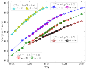
Several key techniques and improvements are applied in our AFQMC simulations. First, we apply the Fast Fourier Transform (FFT) in the propagation (sequential product) of matrices. Within the unitary transformation matrix between - and -space, we arrive at with , where is the band dispersion defined in Sec. II A. Then we have , which explicitly modifies the propagation of matrix by multiplying diagonal matrices in both - and -space plus several FFT operations. This technique implements the diagonal properties of both in -space (under periodic boundary conditions) and in -space (with local interactions). In practical simulations, the FFT operations are realized with standard library (such as FFTW). The computational effort of the matrix propagations can then be reduced to from the conventional scaling. Second, we implement the delayed update [70] and single -line global update [69]. The former is an accelerated way of doing local update, while the latter is a carefully designed cluster update to alleviate the possible ergodicity problem in AFQMC simulations. Delayed update applies rank- Sherman-Morrison updating scheme (with as a predetermined number) instead of the rank-1 formula used in local update, and the acceleration originates from matrix-matrix operation over times of individual matrix-vector operations. This procedure does not alter the Monte Carlo sampling or its statistical efficiency, but instead it reduces the prefactor of the computational scaling [as ] of local update. For every -line global update, we simply choose a lattice site and flip all the auxiliary fields along the imaginary time direction. Figure 5 plots the overall acceptance ratio of this global update for different simulation parameters. We can see that it can still reach for system with and , and it further grows for higher temperature and stronger interaction. Thus, this global update surely improves the efficiency of the imporatance sampling. Pratically, one Monte Carlo sweep in AFQMC simulations contains sweep of local updates, -line global update, and sweep of local updates. , we use column-pivoted QR algorithm for stabilizing the matrix products, and successively a highly stable formalism to obtain the static single-particle Green’s function matrix (with details presented in Ref. 71). Moreover, we compute (for a specific configuration) at from scratch after the numerical stabilization procedure as
| (7) |
The chemical potential term is seperated from the hopping terms in matrix to relieve the ill condition of the matrices, and make the numerical simulations more stable. This improvement is quite important for low filling systems with large , and it allows for AFQMC simulations at lower temperatures. Fourth, for dilute systems, we can apply our recent progress in AFQMC [42] as the speedup algorithm with overall computational scaling .
All the above techniques largely extends the capabilty of finite-temperature AFQMC method, and allow us to obtain results with satisfying precision of system for the 2D Hubbard model in Eq. (1) using moderate computational resource. For example, such system with and costs CPU hours, which produces the results with relative errors for the condensate fraction and on-site pairing correlator. Besides, all these improvements can be easily implemented in AFQMC simulations of other more complicated systems, such as the spin-orbit coupled Hubbard model [75].
II.3 C. Physical observables
Condensate fraction is the key quantity we use to characterize the pairing properties as well as the BKT transition in this work. It can be computed from the pairing matrix in momentum space [61, 42, 43] as
| (8) |
with denoting the -space spin-singlet pairing operator with zero center-of-mass momentum. Thus, the above pairing matrix can be taken as the dominant component of the two-body density matrix related to the off-diagonal long-range order [46, 47] for attractive Hubbard model. Its leading eigenvalue is associated with the condensate fraction as , meaning the fraction of Bose-condensed fermion pairs. The corresponding eigenstate of is the momentum-space pair wave function whose square identifies the probability of fermions with momentum participating the pairing. Its Fourier transform reflects the size distribution of Cooper pairs. In AFQMC simulations, we measure for a specific configuration applying Wick decomposition directly from the -space single-particle Green’s function matrix , which is calculated by FFT of the -space matrix in Eq. (7).
The other quantities for the pairing pheomena is the pairing correlation function and structure factor for on-site spin-singlet Cooper pairs, which is widely studied in previous work [36, 39]. Here we define the pairing operator as , and then the correlation function and the corresponding structure factor can be expressed as and . From , we can identify the on-site pairing correlator as , and at is the magnitude of the long-range pairing order for the ground state. The calculation of in AFQMC is straightforward from the -space matrix.
The pairing matrix in Eq. (8) formally resembles the pairing structure factor . Physically, Cooper pairs with different sizes including local and nonlocal ones should coexist in attractive Hubbard model at low temperature regime [74]. However, the operator for only accounts for the local Cooper pairs, while the for directly probe the -space pairing and thus contains the information of Cooper pairs with various sizes. As a result, togather with the condensate fraction and pair wave function should be a more complete way to characterize the pairing properties for the system of attractive fermions.
Another important observable related to superconductivity and superfluidity is the superfluid density (also called “helicity modulus”). It was found [44, *Scalapino1993] that this quantity can be computed with the dynamic current-current correlation function. The current operator is defined as with representing the unit lattice space in -direction. Then we can obtain its dynamic correlation as with . Then we can reach the imaginary-frequency correlator in momentum space via Fourier transformations as
| (9) |
with . Then the superfluid density can be expressed as
| (10) |
The first term in Eq. (9) actually equals the opposite of kinetic energy associated with the x-oriented links as . In practical AFQMC calulations, we first measure the real-space dynamic current-current correlation function for each configuration using standard Wick decomposition, and then transform it into the momentum space as , and finally obtain the imaginary-frequency result via another Fourier transformation. For finite system with linear system size , we replace the and in Eq. (9) by and in the calculations. Typically, the results dynamic current-current correlation and thus superfluid density are rather noisy due to the much heavier computational cost of calculating dynamic properties in AFQMC method. In this work, we have reached (with ) results for the superfluid density.
II.4 D. Analysis for the finite-size effect of pairing correlator
In superfluid phase, the on-site pairing correlation function , as defined in Sec. II C for 2D systems, should decay algebraically in large limit, i.e., with at and the critical exponent at the BKT transition point. Note that, within translational symmetry and periodic boundary conditions, only depends on the distance . For this case, we can decompose into two seperate regions as and , which satisfies
| (11) |
where is a parameter dependent function. At thermodynamic limit (TDL), the pairing correlator can be expressed as
| (12) | ||||
We have considered the fact that, for a finite system with , the largest distance should be proportional to , and assign the upper limit of integral as with . In the last equality of Eq. (12), the first integral with the integrand should produce some contant , which should finally be independet of (with increasing ). For the second integral, we can substitute and evaluate it as
| (13) |
Then in Eq. (12) can be simplied as
| (14) |
It is clear that, the first term (in red) is the leading contribution of (), while the second term (in blue) is the subleading correction (). As a result, Eq. (14) not only illustrates the algebraic decay of versus in large regime, but also explains its severe finite-size effect which originates from the subleading correction term. This result can serve as the mathematical explanation for the observation in our AFQMC simulations.
II.5 E. AFQMC simulation setup
Our calculations have reached system with lowest temperature , which is significantly larger than ever before. We adopt for , for and for , for which the Trotter error is eliminated from varying tests. We apply periodic boundary conditions in both directions for all the calculations. As for the statistics, we typically ensure that the relative errors of condensate fraction and the pairing correlator fall in between and .
III III. Supplementary results for fixed calculations
In this section, we first show the illustrative results of condensate fraction and pair wave function in Sec. III A, and then present the additional results from AFQMC simulations with fixed for the main text, including with and with in Sec. III B, Sec. III C, Sec. III D, and Sec. III E. For such calculations, the fermion filling changes with both temperature and system size and it reaches converged value with large enough system size. As a summary, we present all the results of fermion filling and double occupancy for the above simulations in Sec. III F.
III.1 A. Illustrative results of condensate fraction and pair wave function
We first take system with as an example to illustrate the high-precision AFQMC results of condensate fraction and pair wave function, as shown in Fig. 6.

The vanishing condensate fraction at high temperature regime indicates the normal phase. With decreasing temperature, the condensate fraction plotted in Fig. 6(a) monotonically grows and develops an inflection point, which can be taken as a signature of entering the superfluid phase. As a comparison, we have also included the results for and at for the same filling as at the same temperature. These results reveal increasing from weak to strong interactions.
The pair wave function in both momentum-space as and real-space as for specific parameters are presented in Fig. 6(b) and (c), respectively. The results have prominent peaks around Fermi surfaces, which numerically validates the basic picture of BCS theory stating that the pairing is mainly contributed by the fermions around Fermi surfaces for weakly interacting regime. The corresponding manifests dominating contribution from local pairing around , and then exhibits a wave structure in extended regime with periodicity which is also consistent with BCS theory. The results also clearly demonstrates the contribution of nonlocal fermion pairing which is completely neglected in the definition of the pairing correlator . These features of and become more significant for lower temperature (as shown for ) and weaker interaction (such as in spite of the tiny ). With increasing , the pairing is more extended in momentum space as is surpressed and scattered to other momentum, and in real space the Cooper pairs gradually evolves into tightly bounded molecules as shrinks to . This is the BCS-BEC crossover which has been extensively studied in interacting Fermi gas with contact attraction [61, 43].
These illustrative results in Fig. 6 explicitly shows that the combination of condensate fraction and pair wave functions captures the full pairing structure in the attracive fermion systems.
III.2 B.
Most of the numerical results for this parameter set is already presented in the main text. Here we present more results of comparisons between the condensate fraction and on-site pairing correlator .

In Fig. 7, we present the rescaled results of condensate fraction and pairing correlator as and versus the linear system size in the log-log plot, with the power-law fittings for and exponential fittings for . The gray horizontal dash-dot lines with seperates the superfluid and normal phases. It is clear that the condensate fraction results within present the same bounded range of as that considering the large system sizes. The results instead renders within .
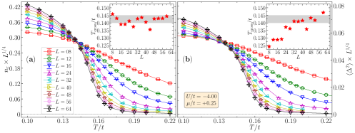
In Fig. 8, we plot the rescaled results of and versus temperature. From the finite-size scaling theory, the cross points between such results from different system sizes should converge to along with increasing . As ploted in the inset for condensate fraction, the cross points of results from and has little variation and are quite consistent with the bounded range (). As a comparison, the cross point of converges very slowly and it is obviously smaller than the results of . These results again show the significant finite-size effect in the pairing correlator.
In the inset of Fig.1 (a) in main text, we present the scaling of the exponent to extract the BKT transition temperature. As mentioned in the main text, this quantity is equal to at the transition point and it is smaller than in the superfluid phase. We find that as this exponent satisfy a linear scaling with temperature. Such an extrapolation to results in the transition temperature , consistent with the data collapse and logarithmic scaling of finite-size BKT transition temperature.
III.3 C.
Here we present similar results for , including temperature and size dependences of condensate fraction and pairing correlator, data collapse, and the energy results.

Figure 9 plots all the results of condensate fraction and pairing correlator for . The monotonically increasing with lowering temperature also shows an inflection point in the mediate temperature. The rescaled results of and versus in Fig. 9(b) and (c) indicate the bounded range of transition temperature as . Consistent results of the exponent extracted from both quantities again confirms the same size scaling behaviors of and . Similar to the case in Sec. III B, the strong finite-size effect in is pretty clear as shown in Fig. 9(c), for which the results obviously deviate from the scaling behavior of results. If the simulations are limited to and one only computes , the result of should be obtained. Instead, the condensate fraction shows much better scaling behavior and results can already reach the correct bounded range of . A further scaling, similar to that in the inset of Fig.1 (a) in main text, presents the transition temperature as .
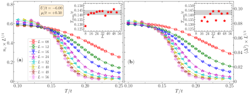
In Fig. 10, we plot the rescaled results of and versus temperature, with the cross points of results from and presented in the insets. Almost all of the crossing temperatures for condensate fraction fall into the correct bounded range of , which the fluctuation of cross points for pairing correlator at lower temperatures is prominent.
In Fig. 11, we plot the data collapse results for and . In the fitting process, we use the numerical data of for and of for , respectively. These two quantities present the BKT transition temperature and , which are well consistent with the bounded range () shown in Fig. 9 and the result from scaling. The results clearly acquires a better data collapse quality than .
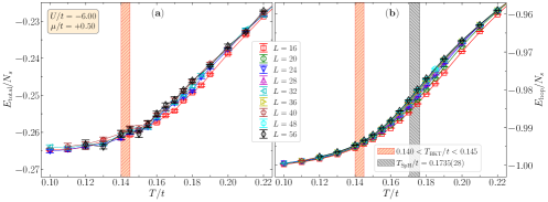
In Fig. 12, we show the results of total energy and kinetic energy versus temperature for . For this case, the finite-size results of total energy are quite noisy as shown in Fig. 12(a), prohibiting us from performing the extrapolations and obtaining precise results of specific heat. Instead, we find that kinetic energy also grows an inflection point (corresponding to the peak location of ) and its location explicitly converges with as . For case, we have verified that the peak location of and are very close. So here we approximately take as the specific heat anomaly temperature as , which leads to a slight larger ratio of than that of case.
III.4 D.
Here we present similar results for , including temperature and size dependences of condensate fraction and pairing correlator and the specific heat results. Especially, for this case, we have also computed the superfluid density and determined from this quantity.

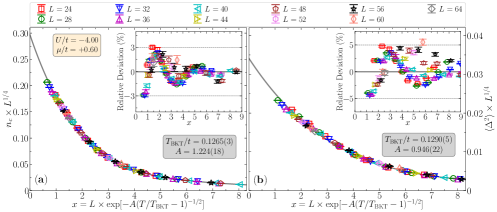
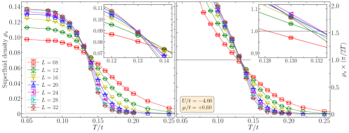
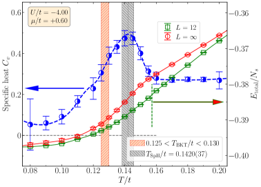
Figure 13 plots all the results of condensate fraction and pairing correlator for . As shown in panel (b), the algebraic scaling in superfluid phase and exponential decaying in normal state of is clear, which results in the bounded range of the transition temperature as . Similar scalings and consistent results of for the pairing correlator can only be reached for results, showing even more severe finite-size effect than that for case. This is attributed to the smaller fermion filling of this case, for which the nonlocal fermion pairing have larger contributions and thus makes the finite-size effect in on-site pairing correlator more significant. If the simulations are limited to and one only computes , the result of should be obtained. Instead, the condensate fraction can still reach the correct range of within results. A further scaling presents the transition temperature as .
Figure 14 plots the data collapse results for and for . These two quantities present the BKT transition temperature and , which are consistent with the bounded range shown in Fig. 13 and the result from scaling.
In Fig. 15, we present the AFQMC results of superfluid density versus temperature for . According to BKT theory, this quantity should acquire a universal jump at the BKT transition point. However, due to the finite-size simulations, we can only obtain continuous results of across the transition, and we can see that the curve of becomes more and more sharp with increasing system size. For , the AFQMC results of are quite noisy at low temperatures, but the results from and show convergence at . Besides, also reach convergence with temperature for , indicating that the superfluid density is about even for the ground state.
There are several ways to extract the BKT transition temperature from superfluid density. First, the crossing points of from different system sizes as shwon in Fig. 15(a) and its inset should converge to towards the thermodynamic limit, resulting in the jump of and the transition point. We can see that for , the crossing points almost converge and resides in the range of , which is well consistent with that obtained from the size scaling of condensate fraction in Fig. 13(b). Second, superfluid density at just below the transition temperature satisfies the relation . Based on this relation, we can take the crossing points of with unity as the finite-size transition temperature [24], and this result should also satisfy the logarithmic correlation relation . From the results shown in Fig. 15(b), from such crossing analysis showes nonmotonic finite-size effect, as it first increases from to and then decreases with . The crossing point of is . Performing AFQMC calculations of dynamic correlations for will surely consume much more computational resources. Considering the moving slow convergence of this crossing point with increasing system size, the final result from this method should also be consistent with the bounded range of .
In Fig. 16, we show the results of specific heat and total energy per site for . A clear peak in results of specific heat appears at , above the BKT transition. The cubic-spline fitting process and numerical differentiation calculation for the total energy present consistent results for this specific heat anomaly as . We also note that the height of the peak in specific heat here is smaller than that for .
III.5 E.
Here we present similar results for , including temperature and size dependences of condensate fraction and pairing correlator and the specific heat results.

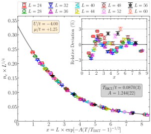
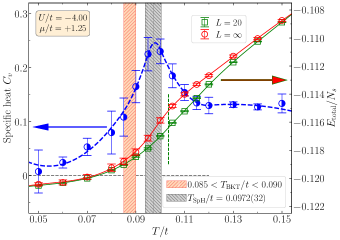
Figure 17 plots all the results of condensate fraction and pairing correlator for . As shown in panel (b), the algebraic scaling in superfluid phase and exponential decaying in normal state of is clear, which results in the bounded range of the transition temperature as . On the other hand, the on-site pairing correlator gets too small for this case, due to the rather small filling . From Fig. 17(c), we can see that for reaches minimum at and almost reach plateau with even larger system size. This means that the results of still suffer strong finite-size effect. For this low filling case, the condensate fraction also show some finite-size effect for , but it is still much better than that of . A further scaling presents the transition temperature as .
Figure 18 plots the data collapse results for for . The fitting with least-squares criterion presents the transition temperature , which is consistent with the bounded range shown in Fig. 17 and the result from scaling.
In Fig. 19, we show the results of specific heat and total energy per site for . A clear peak in results of specific heat appears at , above the BKT transition. The cubic-spline fitting process and numerical differentiation calculation for the total energy present consistent results for this specific heat anomaly as . We also note that the height of the peak in specific heat gradually decreases for from to and to as towards the lower filling regime.
III.6 F. Summary of all the AFQMC simulations
Here we present a summary for all the AFQMC simulation results in Sec. II, and also present the results of fermion filling and double occupancy, which might be used as benchmark for future experiments, other theoretical studies and many-body calculations.
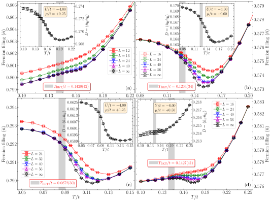
We have mainly performed the AFQMC simulations for 2D attracive Hubbard model for with fixed and with fixed . Our calculations reach the linear system size with the lowest temperature . We mainly concentrate on the condensate fraction and on-site pairing correlator around the BKT transition. All of our numerical results reveal that these two quantities have the same size scaling behaviors, i.e., algebraic scaling () in superfluid phase and exponential decaying in normal state. We also find that the extensively studied pairing correlator suffers from severe finite-size effect (as deviation from the correct scaling in small sizes). As a comparison, the condensate fraction shows significantly better size scaling in small systems, rendering it as a more appropriate quantity to determine the BKT transition temperature.
In Fig. 20, we present the summarization results of fermion filling (main plots) and double occupancy (the inset) versus temperature and system size for all the four sets of parameters in Sec. III B Sec. III E. The results are obtained from finite-size extrapolations. The corresponding BKT transition temperatures are also presented in the plots.
IV IV. Supplementary results for fixed fermion filling calculations
In this section, we further present the results of AFQMC simulations with fixed fermion filling . Results for two representative different interaction strengths and are obtained. These results also explicitly shows that condensate fraction and on-site pairing correlator have the same size scaling, with the finite-size effect in the former is significantly smaller than the latter.
IV.1 A.

Figure 21 plots all the results of condensate fraction and pairing correlator for . As shown in panel (b), the algebraic scaling in superfluid phase and exponential decaying in normal state of is clear, which results in the bounded range of the transition temperature as . On the other hand, the on-site pairing correlator suffers severe finite-size effect and only results can reach the correct algebraic scaling. If the simulation is limited to , the result of should be obtained. Instead, the condensate fraction results can correctly present the transition temperature within . A further scaling for the exponent (using the results of and ) determines the transition temperature as .
IV.2 B.

Figure 22 plots all the results of condensate fraction and pairing correlator for . As shown in panel (b), the algebraic scaling in superfluid phase and exponential decaying in normal state of determine the bounded range of the transition temperature as . For this case, the finite-size effect in is moderate as results can reach the correct algebraic scaling and present consistent exponents with those from for . This can be attributed to the strong attractive interaction, for which the contribution from nonlocal pairing in the system is rather small. A further scaling for the exponent (using the results of and ) determines the transition temperature as .