Minimax Rate-Optimal Algorithms for High-Dimensional Stochastic Linear Bandits

Abstract

We study the stochastic linear bandit problem with multiple arms over $T$ rounds, where the covariate dimension $d$ may exceed $T$, but each arm-specific parameter vector is $s$-sparse. We begin by analyzing the sequential estimation problem in the single-arm setting, focusing on cumulative mean-squared error. We show that Lasso estimators are provably suboptimal in the sequential setting, exhibiting suboptimal dependence on $d$ and $T$, whereas thresholded Lasso estimators—obtained by applying least squares to the support selected by thresholding an initial Lasso estimator—achieve the minimax rate. Building on these insights, we consider the full linear contextual bandit problem and propose a three-stage arm selection algorithm that uses thresholded Lasso as the main estimation method. We derive an upper bound on the cumulative regret of order $s(\log s)(\log d+\log T)$, and establish a matching lower bound up to a $\log s$ factor, thereby characterizing the minimax regret rate up to a logarithmic term in $s$. Moreover, when a short initial period is excluded from the regret, the proposed algorithm achieves exact minimax optimality.

and

1 Introduction

With the rapid growth of data from sources such as mobile applications and healthcare monitoring, streaming data has become an important focus in modern statistical analysis [35, 24]. Streaming data refers to data arriving continuously over time, often in large volumes and at high velocity. In these settings, statistical procedures must operate in real time, updating models and making decisions as new observations arrive. In this work, we focus on multi-armed bandit (MAB) problems, a fundamental example of sequential decision-making, with wide applications including online advertising [13], personalized medicine [37], and recommendation systems [25].

Classical MAB problems, introduced by [38] and formalized by [32], concern the sequential selection of arms with unknown mean rewards to maximize cumulative reward—or equivalently, to minimize cumulative regret relative to always choosing the best arm. Foundational algorithms such as upper confidence bound [23, 5], Thompson sampling [2], and information-directed sampling [34] achieve near-optimal regret guarantees in this setting [4, 11]. However, these models do not incorporate contextual information, or covariates, which can greatly enhance decision-making. The inclusion of context leads to diverse modeling frameworks: parametric [26] vs. nonparametric [28], linear [1, 16, 7, 8] vs. nonlinear [20, 14], and stochastic [16, 7, 8] vs. adversarial [6, 21] environments; see [24] for a comprehensive overview. Given the breadth of the literature, we begin by precisely defining our setting and focusing on the most relevant prior work.

Suppose there are $K$ arms, each associated with an unknown $d$-dimensional parameter vector $\boldsymbol{\theta}^{(k)}\in\mathbb{R}^{d}$ for $k\in[K]:=\{1,\ldots,K\}$. We consider the following sequential decision-making problem over $T$ rounds. At each round $t\in[T]:=\{1,\ldots,T\}$, a covariate vector $\boldsymbol{X}_{t}\in\mathbb{R}^{d}$ is observed, an arm $A_{t}\in[K]$ is selected, and a reward $Y_{t}\in\mathbb{R}$ is received. The arm selection $A_{t}$ is allowed to depend only on $\boldsymbol{X}_{t}$ and the past history up to time $t-1$, that is, $\{(\boldsymbol{X}_{s},Y_{s},A_{s}):s<t\}$. We assume that the covariate vectors $\{\boldsymbol{X}_{t}:t\in[T]\}$ are independent and identically distributed (i.i.d.) random vectors in $\mathbb{R}^{d}$, and that the expected reward is linear in $\boldsymbol{X}_{t}$ and the parameter of the selected arm:

$$Y_{t}=\boldsymbol{X}_{t}^{\prime}\boldsymbol{\theta}^{(A_{t})}+\epsilon_{t},$$

where $\{\epsilon_{t}:t\in[T]\}$ are i.i.d. zero-mean random variables, independent of $\{\boldsymbol{X}_{t}:t\in[T]\}$. Given an arm selection rule with arm choices $\{A_{t}:t\in[T]\}$, we evaluate its performance using the expected cumulative regret. Specifically, for each $t\in[T]$, define the instantaneous regret: $r_{t}:=\max_{k\in[K]}\boldsymbol{X}_{t}^{\prime}\boldsymbol{\theta}^{(k)}-\boldsymbol{X}_{t}^{\prime}\boldsymbol{\theta}^{(A_{t})}$, which compares the chosen arm to the best possible arm at time $t$. The expected cumulative regret is then defined as $\sum_{t=1}^{T}\mathbb{E}[r_{t}]$. The objective is to find an arm selection rule that minimizes this quantity.

When the covariate dimension $d$ is much smaller than the time horizon $T$, we refer to this as the low-dimensional regime. In this setting, the arm parameters are typically estimated using ordinary least squares (OLS) or ridge regression. [16] proposes a forced sampling strategy based on OLS for the two-arm case ($K=2$), and establishes an upper bound on the cumulative regret of order $O(d^{3}\log T)$ under a margin condition. This condition requires that the probability of $\boldsymbol{X}_{t}$ falling within a distance $\tau$ of the decision boundary $\{\boldsymbol{x}\in\mathbb{R}^{d}:(\boldsymbol{\theta}^{(1)})^{\prime}\boldsymbol{x}=(\boldsymbol{\theta}^{(2)})^{\prime}\boldsymbol{x}\}$ is at most $C\tau$ for any $\tau>0$. This bound is improved to $O(d^{2}\log^{3/2}d\log T)$ in [7]. The work [16] also establishes a lower bound of order $\Omega(\log T)$, which characterizes the optimal dependence on $T$, though the optimal dependence on $d$ remains unresolved. An alternative approach is proposed in [1], where the LinUCB algorithm—based on ridge regression and the principle of upper confidence bounds—is shown to attain a regret upper bound of $O(\log^{2}T)$ [17]. However, [36] demonstrates that LinUCB is suboptimal, and proposes a variant in which the algorithm is truncated at a prescribed time and followed by pure exploitation. The resulting truncated LinUCB algorithm achieves a regret bound of $O(d\log T)$, which is shown to be optimal in both $d$ and $T$.

In this work, we focus on the high-dimensional regime, where the covariate dimension $d$ may substantially exceed the time horizon $T$. Such settings arise in applications where rich contextual features are available but sample sizes are limited due to budget or time constraints [7, 24]. To ensure statistical tractability, we assume that for each arm $k\in[K]$, $\boldsymbol{\theta}^{(k)}$ is $s_{0}$-sparse, meaning that it has at most $s_{0}$ nonzero components. This reflects the standard assumption that only a small subset of covariates is relevant for reward prediction, and is widely used in the high-dimensional bandit literature [7, 18, 27, 30]. Our goal is to characterize the minimax rate of cumulative regret and to develop algorithms that approach this rate.

For any bandit algorithm, a fundamental component is the estimation of the arm parameters. Based on these estimates—and possibly on a quantification of their uncertainty—the algorithm selects an arm to pull. In order to understand the statistical limits of estimation methods in sequential, high-dimensional settings, we first isolate the sequential estimation problem, where a single sparse parameter vector is estimated sequentially without adaptive arm selection. This problem is of independent interest and provides insight into the design of effective arm-selection strategies in the full bandit problem.

1.1 Sequential High-Dimensional Linear Regression

Consider the setting with a single arm, i.e., $K=1$, and denote $\boldsymbol{\theta}^{(1)}$ by $\boldsymbol{\theta}$. At each round $t\in[T]$, we construct an estimator $\hat{\boldsymbol{\theta}}_{t}$ based on the data $\{(\boldsymbol{X}_{s},Y_{s}):s\in[t]\}$ observed up to time $t$. We evaluate the sequence of estimators $\{\hat{\boldsymbol{\theta}}_{t}:t\in[T]\}$ through the cumulative capped mean-square error: $\sum_{t=1}^{T}\mathbb{E}[\min\{\|\hat{\boldsymbol{\theta}}_{t}-\boldsymbol{\theta}\|_{2}^{2},\;\xi\}]$, where $\xi>0$ is a fixed constant; see Section 2.

Since no arm selection is involved, at each round $t\in[T]$, the data $\{(\boldsymbol{X}_{s},Y_{s}):s\in[t]\}$ are i.i.d., allowing us to leverage the extensive literature on fixed-sample high-dimensional linear regression. In particular, the Lasso estimator [39], which minimizes the $\ell_{1}$-penalized least squares criterion, is among the most widely used methods in this setting. For fixed $t=\Omega(s_{0}\log d)$, and under restricted eigenvalue-type conditions, it is well known [41, 42, 45] that the Lasso estimator $\hat{\boldsymbol{\theta}}_{t}^{\textup{Lasso}}$ achieves a mean-squared error of order $O(s_{0}\log d/t)$, which matches the minimax rate. Hence, no estimator can uniformly outperform Lasso over the class of all $s_{0}$-sparse parameter vectors $\boldsymbol{\theta}$ for a fixed $t$. Despite its minimax optimality, many variants of Lasso have been proposed—such as the elastic net [51], group Lasso [47], adaptive Lasso [50], and thresholded Lasso [40, 10]—with the goal of improving instance-specific estimation accuracy or variable selection performance.

Now, in the sequential estimation problem, we may apply the Lasso estimator $\hat{\boldsymbol{\theta}}_{t}^{\textup{Lasso}}$ at each round $t\in[T]$. Summing the upper bound $s_{0}\log d/t$ over $t\in[T]$ yields a cumulative error bound of order $O(s_{0}\log(d)\log(T))$ for the sequence of Lasso estimators. However, it remains unclear whether this bound is tight for Lasso, or whether it coincides with the minimax rate. Importantly, the fact that Lasso is minimax optimal at each fixed time $t\in[T]$ does not imply minimax optimality in terms of cumulative error. The key distinction is that in the sequential setting, the underlying parameter vector $\boldsymbol{\theta}$ is shared across all $T$ rounds, whereas in the fixed-sample minimax theory, the worst-case $\boldsymbol{\theta}$ may vary across rounds.

Our contributions. First, we establish in Theorem 5 that the worst-case cumulative error of Lasso estimators is of order $\Omega(s_{0}\log(d)\log(T))$, indicating that the previously derived upper bound is tight. Second, we consider the OPT-Lasso estimators [40, 10], which first threshold an initial Lasso estimator and then apply ordinary least squares to the selected support. In Theorem 1, we provide an instance-specific upper bound on the mean-squared error of OPT-Lasso for a fixed $t\in[T]$, which explicitly characterizes the impact of the nonzero components of $\boldsymbol{\theta}$, and leads to a cumulative error bound of order $s_{0}(\log d+\log T)$. A key technical tool is the recent $\ell_{\infty}$ bound for Lasso estimators established in [9]. Third, we establish a matching lower bound that holds uniformly over all permissible estimators. Specifically, we lower bound the minimax rate via Bayesian risks by constructing two families of prior distributions, and show in Theorem 3 that any permissible sequence of estimators must incur a worst-case cumulative error of order at least $s_{0}(\log d+\log T)$.

These results characterize the minimax rate and demonstrate that Lasso estimators are provably suboptimal in the sequential setting, while OPT-Lasso estimators are minimax optimal. The sequential estimation problem is of independent interest, and our analysis further indicates that OPT-Lasso is broadly preferable to Lasso in sequential tasks—for example, in the bandit setting.

1.2 High-dimensional Linear Contextual Bandits

Next, we focus on the bandit setting with at least two arms, i.e., $K\geq 2$, under the high-dimensional linear contextual framework. In this setting, [7] extends the “forced sampling” strategy of [16] by replacing ridge regression with Lasso estimators, and establishes an upper bound on the expected cumulative regret of order $O(s_{0}^{2}(\log d+\log T)^{2})$. Subsequently, [46] proposes an algorithm based on a two-step weighted Lasso estimator, achieving an improved upper bound of order $O(s_{0}^{2}(s_{0}+\log d)\log T)$. More recently, [3] introduces a pure exploitation algorithm based on thresholded Lasso estimators. Under the assumptions that (i) $s_{0}$ is a constant, and (ii) the nonzero components of $\{\boldsymbol{\theta}^{(k)}:k\in[K]\}$ are bounded away from zero by a constant, [3] derives an upper bound on the cumulative regret of order $O((\log\log d)\log d+\log T)$. It is important to note that all of the aforementioned results rely on the margin condition, which enables regret bounds that are logarithmic in the time horizon $T$. Without this condition, the cumulative regret grows polynomially in $T$; see, for instance, [22, 27, 3, 30].

As for lower bounds, the result in the low-dimensional regime [36] implies a trivial lower bound of order $\Omega(s_{0}\log T)$, which corresponds to the case where the support of $\boldsymbol{\theta}^{(k)}$ is known for $k\in[K]$. However, it remains unclear whether this lower bound is tight in the high-dimensional setting or what the minimax regret rate should be in general.

Our contributions. First, building on insights from the sequential estimation problem, we propose a three-stage algorithm. In Stage 1, spanning from round $t=1$ to $\gamma_{1}$, arms are selected uniformly at random from $[K]$. In Stage 2, from round $\gamma_{1}+1$ to $\gamma_{2}$, we estimate the arm parameters using the Lasso method and select the arm that maximizes the estimated reward based on these estimates. In Stage 3, from round $\gamma_{2}+1$ to $T$, we replace the Lasso estimators with OPT-Lasso estimators and continue to perform pure exploitation as in Stage 2. To improve computational efficiency, the estimators in Stages 2 and 3 are updated periodically rather than at every round. As discussed in Section 3, we choose $\gamma_{1}$ to be of order $s_{0}\log(dT)$ and $\gamma_{2}$ to be of order $s_{0}^{5}\log(dT)$, so that Stage 3 dominates the time horizon and the algorithm predominantly relies on OPT-Lasso estimators. The motivation for introducing Stage 2 is discussed in Section 3.

Second, in Theorem 6, we establish an upper bound of order $O(s_{0}(\log s_{0})(\log d+\log T))$ on the overall cumulative regret of the proposed three-stage algorithm. Furthermore, if the cumulative regret is computed starting from round $Cs_{0}^{5}\log(dT)$, for a sufficiently large constant $C$, the upper bound improves to $O\left(s_{0}(\log d+\log T)\right)$, removing the $\log s_{0}$ factor. We emphasize that our analysis allows $s_{0}$ to grow with $d$ and $T$, and does not require any “beta-min” type condition as in [3]. See more discussions in Subsection 3.2.

Third, in Theorem 7, we establish a lower bound of order $s_{0}(\log d+\log T)$ for the cumulative regret starting from round $Cs_{0}^{5}\log(dT)$, uniformly over all permissible rules and for any constant $C>0$. This result automatically implies a lower bound of the same order for the overall cumulative regret. As a consequence, we characterize the minimax rate of the overall cumulative regret, up to a $\log s_{0}$ factor, and show that the proposed algorithm is nearly minimax optimal. Moreover, if the initial period of length $O(s_{0}^{5}\log T)$ is ignored, the minimax rate is $s_{0}(\log d+\log T)$, which is attained by the proposed algorithm.

Finally, we show in Theorem 10 that using Lasso instead of OPT-Lasso leads to provably suboptimal performance, which demonstrates the necessity of using thresholded estimators in this setting. In addition, simulation results further demonstrate the favorable performance of the proposed three-stage algorithm compared to alternative approaches.

1.3 Paper Organization and Notations

In Section 2, we study the sequential high-dimensional linear regression problem. The Lasso and OPT-Lasso estimators are formally introduced in Subsection 2.1. In Subsection 2.2, we characterize the minimax rate and show that OPT-Lasso achieves minimax optimality. The suboptimality of Lasso is analyzed in Subsection 2.3, with supporting simulation results presented in Subsection 2.4.

Section 3 turns to the bandit setting. A three-stage algorithm is introduced in Subsection 3.1, and its cumulative regret is analyzed in Subsection 3.2, where we also establish nearly matching lower bounds. The suboptimality of Lasso in this setting is analyzed in Subsection 3.3. Corresponding simulation results are presented in Subsection 3.4. The proof of the regret bounds is provided in Subsection 3.5. We conclude in Section 4, and include additional proofs and simulation results in the Appendix.

Notations. The abbreviation “i.i.d.” stands for “independent and identically distributed”. For each $n\in\mathbb{N}:=\{1,2,\ldots\}$, we denote by $[n]=\{1,\cdots,n\}$, and by $\boldsymbol{0}_{n}$ the zero vector in $\mathbb{R}^{n}$. For $a,b\in\mathbb{R}$, $a\vee b=\max\{a,b\}$ and $a\wedge b=\min\{a,b\}$. $\mathbbm{1}\{R\}$ denotes the indicator function of event $R$; that is, $\mathbbm{1}\{R\}$ is $1$ (resp. $0$) if $R$ is true (resp. false). Let $\{a_{T};T\in\mathbb{N}\}$ be a sequence of real numbers. We denote $a_{T}=O(T)$ (resp. $a_{T}=\Omega(T)$) if there exists a constant $C>0$, that does not depend on $T$, such that $a_{T}\leq CT$ (resp. $a_{T}\geq C^{-1}T$).

Unless otherwise specified, all vectors are assumed to be column vectors. For a vector $\boldsymbol{v}=(v_{1},\ldots,v_{d})^{\prime}\in\mathbb{R}^{d}$, the $\ell_{p}$ norm is defined as $\|\boldsymbol{v}\|_{p}=(\sum_{i\in[d]}|v_{i}|^{p})^{1/p}$ for $1\leq p<\infty$. The $\ell_{0}$ “norm” $\|\boldsymbol{v}\|_{0}=|\{j\in[d]:\boldsymbol{v}_{j}\neq 0\}|$ denotes the number of nonzero components in $\boldsymbol{v}$, and the $\ell_{\infty}$ norm is given by $\|\boldsymbol{v}\|_{\infty}=\max_{j\in[d]}|v_{j}|$. For a matrix $\boldsymbol{A}\in\mathbb{R}^{m\times n}$, define the matrix norms ${\left|\kern-1.07639pt\left|\kern-1.07639pt\left|\boldsymbol{A}\right|\kern-1.07639pt\right|\kern-1.07639pt\right|}_{1}=\max_{1\leq j\leq n}\sum_{i=1}^{m}|\boldsymbol{A}_{i,j}|$, ${\left|\kern-1.07639pt\left|\kern-1.07639pt\left|\boldsymbol{A}\right|\kern-1.07639pt\right|\kern-1.07639pt\right|}_{\infty}=\max_{1\leq i\leq m}\sum_{j=1}^{n}|\boldsymbol{A}_{i,j}|$, and ${\left|\kern-1.07639pt\left|\kern-1.07639pt\left|\boldsymbol{A}\right|\kern-1.07639pt\right|\kern-1.07639pt\right|}_{\textup{max}}=\max_{1\leq i\leq m,1\leq j\leq n}|\boldsymbol{A}_{i,j}|$. If $\boldsymbol{A}$ is symmetric and positive semidefinite, denote by $\lambda_{\min}\left(\boldsymbol{A}\right)$ and $\lambda_{\max}\left(\boldsymbol{A}\right)$ the smallest and largest eigenvalue of $\boldsymbol{A}$ respectively, and by $\boldsymbol{A}^{1/2}$ a symmetric matrix such that $\boldsymbol{A}^{1/2}\boldsymbol{A}^{1/2}=\boldsymbol{A}$. Given subsets $S_{1}\subseteq[m]$ and $S_{2}\subseteq[n]$, denote by $\boldsymbol{A}_{S_{1},S_{2}}\in\mathbb{R}^{|S_{1}|\times|S_{2}|}$ the submatrix of $\boldsymbol{A}$ consisting of the rows indexed by $S_{1}$ and the columns indexed by $S_{2}$. We abbreviate $\boldsymbol{A}_{[m],S_{2}}$ as $\boldsymbol{A}_{S_{2}}$. For $\boldsymbol{A}\in\mathbb{R}^{m\times n}$, denote its transpose by $\boldsymbol{A}^{\prime}$.

2 Sequential High-Dimensional Linear Regression

In this section, we focus on the sequential high-dimensional linear regression problem. Specifically, let $T$ be the total number of rounds, which is also called the horizon. At each round (or time) $t\in[T]$, a pair of observations $(Y_{t},\boldsymbol{X}_{t})\in\mathbb{R}\times\mathbb{R}^{d}$ is collected, which is assumed to follow a linear regression model with an unknown parameter $\boldsymbol{\theta}\in\mathbb{R}^{d}$ and an observation noise $\epsilon_{t}\in\mathbb{R}$, that is,

$$Y_{t}=\boldsymbol{X}_{t}^{\prime}\boldsymbol{\theta}+\epsilon_{t}.$$

Assume that $\{\boldsymbol{X}_{t}\in\mathbb{R}^{d}:t\in[T]\}$ are i.i.d. random vectors drawn from the multivariate normal distribution $\mathcal{N}(\mathbf{0}_{d},\boldsymbol{\Sigma})$, where $\mathbf{0}_{d}\in\mathbb{R}^{d}$ is the mean vector, and $\boldsymbol{\Sigma}\in\mathbb{R}^{d\times d}$ is the covariance matrix. Further, assume that $\{\epsilon_{t}\in\mathbb{R}:t\in[T]\}$ are i.i.d. random variables drawn from the normal distribution $\mathcal{N}(0,\sigma^{2})$.

Let $S$ denote the support of $\boldsymbol{\theta}=(\boldsymbol{\theta}_{1},\ldots,\boldsymbol{\theta}_{d})^{\prime}$, i.e., $S=\{j\in[d]:\boldsymbol{\theta}_{j}\neq 0\}$. We define $s_{0}=|S|\vee 1$, so that $s_{0}=1$ when $S$ is empty. Denote by $\boldsymbol{\Theta}_{d}[s]:=\{\boldsymbol{\theta}\in\mathbb{R}^{d}:\|\boldsymbol{\theta}\|_{0}\leq s\}$ the set of all $s$-sparse vectors. Thus, $\boldsymbol{\theta}\in\boldsymbol{\Theta}_{d}[s_{0}]$. We focus on the high-dimensional regime, where the covariate dimension $d$ is potentially much larger than the horizon $T$, i.e. $d\gg T$, while only a few covariates capture the overall impact on the responses, i.e., $s_{0}\ll d$.

For each time $t\in[T]$, we denote by $\widehat{\boldsymbol{\theta}}_{t}$ an estimator of the unknown parameter $\boldsymbol{\theta}$ based on the currently available observations $\boldsymbol{X}_{[t]}=(\boldsymbol{X}_{1},\cdots,\boldsymbol{X}_{t})^{\prime}$ and $\boldsymbol{Y}_{[t]}=(Y_{1},\cdots,Y_{t})^{\prime}$. Our goal is to find a sequence of estimators $\{\widehat{\boldsymbol{\theta}}_{t}:t\in[T]\}$ to minimize the cumulative capped mean-square error

$$\sum_{t=1}^{T}\mathbb{E}\left[\|\widehat{\boldsymbol{\theta}}_{t}-\boldsymbol{\theta}\|_{2}^{2}\wedge\xi\right],$$

where $\xi>0$ is an arbitrary user-specified parameter. To make the dependence on $\boldsymbol{\theta}$ explicit, we use the notation $\mathbb{E}_{\boldsymbol{\theta}}$ in place of $\mathbb{E}$ when needed.

Remark 1.

In high-dimensional regression literature, estimation error bounds are typically stated with high probability: for each $t\in[T]$, there exists a high-probability event on which $\|\widehat{\boldsymbol{\theta}}_{t}-\boldsymbol{\theta}\|_{2}$ is controlled. Introducing a cap parameter allows these bounds to be converted into expected error bounds.

In the sequential estimation problem considered in this section, no arm selection is involved. As a result, for each round $t\in[T]$, the observations $\{(X_{s},Y_{s}):s\in[t]\}$ are i.i.d. and can be treated as a fixed-sample problem. However, the problems across rounds are coupled due to the shared parameter $\boldsymbol{\theta}$ and the cumulative nature of the performance criterion.

2.1 Lasso and OPT-Lasso: Fixed-Sample Discussion

In this subsection, we discuss two well-known procedures in the fixed-sample high-dimensional linear regression literature. We start with the Lasso estimator [39], which applies $\ell_{1}$-regularization and is defined as follows.

Definition 1.

Let $n\in\mathbb{N}$. Given a matrix $\boldsymbol{X}\in\mathbb{R}^{n\times d}$, a vector $\boldsymbol{Y}\in\mathbb{R}^{n}$ and a regularization parameter $\lambda>0$, the Lasso estimator $\widehat{\boldsymbol{\theta}}^{\textup{Lasso}}_{n}(\boldsymbol{X},\boldsymbol{Y},\lambda)$ is defined as

$$\widehat{\boldsymbol{\theta}}^{\textup{Lasso}}_{n}(\boldsymbol{X},\boldsymbol{Y},\lambda):=\operatorname*{argmin}_{\boldsymbol{\beta}\in\mathbb{R}^{d}}\left\{\frac{1}{2n}\|\boldsymbol{Y}-\boldsymbol{X}\boldsymbol{\beta}\|_{2}^{2}+\lambda\|\boldsymbol{\beta}\|_{1}\right\}.$$

The Lasso estimator is known to be minimax optimal for a fixed sample size. Specifically, see Example 7.14 in [45] for a high probability upper bound on the $\ell_{2}$ estimation error, and Theorem 1(b) in [29] for a matching minimax lower bound. Therefore, it may be surprising that, as we show in section 2.3, the Lasso estimator becomes suboptimal in the sequential setting in terms of the worst-case cumulative error. We note that this is not contradictory. For a general sequence of estimators $\{\widehat{\boldsymbol{\theta}}_{t}:t\in[T]\}$, we have

$$\sup_{\boldsymbol{\theta}\in\boldsymbol{\Theta}_{d}[s_{0}]}\sum_{t=1}^{T}\mathbb{E}_{\boldsymbol{\theta}}\left[\|\widehat{\boldsymbol{\theta}}_{t}-\boldsymbol{\theta}\|_{2}^{2}\wedge\xi\right]\leq\sum_{t=1}^{T}\sup_{\boldsymbol{\theta}\in\boldsymbol{\Theta}_{d}[s_{0}]}\mathbb{E}_{\boldsymbol{\theta}}\left[\|\widehat{\boldsymbol{\theta}}_{t}-\boldsymbol{\theta}\|_{2}^{2}\wedge\xi\right].$$

The Lasso estimator achieves minimax optimality for each (sufficiently large) $t$, and is therefore optimal with respect to the criterion on the right-hand side. However, that does not imply its minimax optimality in the sequential setting, since the problems across rounds are coupled by a single $\boldsymbol{\theta}$, as previously discussed.

The suboptimality of Lasso in the sequential setup motivates us to consider another well-known estimator in the fixed-sample literature, which we refer to as OPT-Lasso; see, e.g., Section 7.6 of [12] and [10]. Note that “OPT” stands for “OLS Post Thresholded”.

Definition 2.

Let $n\in\mathbb{N}$. Given a matrix $\boldsymbol{X}\in\mathbb{R}^{n\times d}$, a vector $\boldsymbol{Y}\in\mathbb{R}^{n}$, and two regularization parameters $\lambda,\lambda^{\textup{OPT}}>0$, the OPT-Lasso estimator $\widehat{\boldsymbol{\theta}}^{\textup{OPT}}_{n}:=\widehat{\boldsymbol{\theta}}^{\textup{OPT}}_{n}(\boldsymbol{X},\boldsymbol{Y},\lambda,\lambda^{\textup{OPT}})$ is defined as follows:

1. Compute the Lasso estimator $\widehat{\boldsymbol{\theta}}^{\textup{Lasso}}_{n}(\boldsymbol{X},\boldsymbol{Y},\lambda)$, denoted by $\widehat{\boldsymbol{\theta}}^{\textup{Lasso}}_{n}$;

2. Threshold each component of the Lasso estimator using $\lambda^{\textup{OPT}}$:

   $$\hat{S}^{\textup{OPT}}_{n}:=\left\{j\in[d]:|(\widehat{\boldsymbol{\theta}}^{\textup{Lasso}}_{n})_{j}|>\lambda^{\textup{OPT}}\right\}.$$

3. Apply the ordinary least squares (OLS) procedure using the covariates in $\hat{S}^{\textup{OPT}}_{n}$, and set the remaining coordinates to zero:

   $$(\widehat{\boldsymbol{\theta}}^{\textup{OPT}}_{n})_{\hat{S}^{\textup{OPT}}_{n}}=\min_{\boldsymbol{\beta}\in\mathbb{R}^{\left|\hat{S}^{\textup{OPT}}_{n}\right|}}\left\|\boldsymbol{Y}-\boldsymbol{X}_{\hat{S}^{\textup{OPT}}_{n}}\boldsymbol{\beta}\right\|_{2}^{2},\quad(\widehat{\boldsymbol{\theta}}^{\textup{OPT}}_{n})_{j}=0\text{ for }j\in(\hat{S}^{\textup{OPT}}_{n})^{c}.$$

For a fixed round $t\in[T]$, as discussed in [10], OPT-Lasso achieves the same minimax convergence rate of $O(s_{0}\log d/t)$ as Lasso, while additionally providing improved instance-specific rates by reducing Lasso’s bias. Specifically, if the initial Lasso estimator has the variable screening property—that is, its support contains the true support $S$—then OPT-Lasso has a strictly faster rate of convergence. Moreover, if the support of the initial Lasso estimator is equal to $S$, then OPT-Lasso attains the oracle rate $O(s_{0}/t)$.

The variable screening property of Lasso in general requires the so-called beta-min condition (see (2.23) in [12]) as follows:

$$\min_{j\in S}|\boldsymbol{\theta}_{j}|=\Omega(\sqrt{(s_{0}\log d)/n}),$$ (1)

which ensures that the smallest nonzero coefficient in the true support $S$ is sufficiently large in absolute value. If, with a high probability, the following incoherence condition holds:

$$\max_{i\neq j\in[d]}|n^{-1}\sum_{\ell=1}^{n}{\boldsymbol{X}_{\ell,i}\boldsymbol{X}_{\ell,j}}|=O(1/s_{0}),$$ (2)

then condition (1) can be relaxed as $\min_{j\in S}|\boldsymbol{\theta}_{j}|=\Omega(\sqrt{\log d/n})$ (see Theorem 2 in [10]).

As we will see, in the sequential setup, the beta-min condition is particularly restrictive, and under this condition, it is unclear how to derive the minimax rate; see discussions following Theorem 1 and in Remark 2. In this work, we do not impose “beta-min” type conditions.

In this section, for each time $t\in[T]$, we denote by $\widehat{\boldsymbol{\theta}}^{\textup{OPT}}_{t}$ the OPT-Lasso estimator $\widehat{\boldsymbol{\theta}}^{\textup{OPT}}_{t}(\boldsymbol{X}_{[t]},\boldsymbol{Y}_{[t]},\lambda_{t},\lambda^{\textup{OPT}}_{t})$ and by $\widehat{\boldsymbol{\theta}}^{\textup{Lasso}}_{t}$ the Lasso estimator $\widehat{\boldsymbol{\theta}}^{\textup{Lasso}}_{t}(\boldsymbol{X}_{[t]},\boldsymbol{Y}_{[t]},\lambda_{t})$, where recall that $\boldsymbol{X}_{[t]}$ and $\boldsymbol{Y}_{[t]}$ are the observations available up to time $t$, and $\lambda_{t},\lambda^{\textup{OPT}}_{t}$ are tuning parameters to be specified.

2.2 Minimax Optimality of OPT-Lasso in Sequential Estimation

In this subsection, we show that in the sequential setup, OPT-Lasso achieves minimax optimality with respect to the cumulative capped mean-squared error. Recall that $S$ denotes the support of the unknown parameter $\boldsymbol{\theta}$.

Assumption 1.

Let $L_{0}>0$ be a constant.

1. For $j\in[d]$, $\boldsymbol{\Sigma}_{j,j}\leq 1$.

2. Assume that

   $$\max_{A\subseteq[d]:|A\backslash S|\leq 1\vee(L_{0}s_{0}+1)}\frac{\lambda_{\max}\left(\boldsymbol{\Sigma}_{A,A}\right)}{\lambda_{\min}\left(\boldsymbol{\Sigma}_{A,A}\right)}\leq L_{0}/2,\ \min_{A\subseteq[d]:|A\backslash S|=L_{0}s_{0}+1}\lambda_{\min}\left(\boldsymbol{\Sigma}_{A,A}\right)\geq L_{0}^{-1}.$$

3. If $S$ is non-empty, assume that $L_{0}^{-1}\leq\lambda_{\min}\left(\boldsymbol{\Sigma}_{S,S}\right)\leq\lambda_{\max}\left(\boldsymbol{\Sigma}_{S,S}\right)\leq L_{0}$.

4. $\boldsymbol{\Sigma}$ is invertible, and ${\left|\kern-1.07639pt\left|\kern-1.07639pt\left|\boldsymbol{\Sigma}^{-1}\right|\kern-1.07639pt\right|\kern-1.07639pt\right|}_{\infty}\leq L_{0}$.

Assumption 1 (a) requires that the variances of the covariates are uniformly bounded by a constant, which, without loss of generality, is assumed to be $1$. Assumption 1 (c) ensures that the population covariance matrix of the covariates, when restricted to the support $S$, is non-singular and well-conditioned. Assumption 1 (b) is known as the sparse Riesz condition (see [48, 9]), which controls the range of the eigenvalues of the covariance matrices restricted to subsets containing a bounded number of covariates. This condition ensures that Lasso estimators can recover a model with the correct order of sparsity. Assumption 1 (d) requires that the $\ell_{1}$ norm of each column of $\boldsymbol{\Sigma}^{-1}$ is bounded. This type of condition commonly appears in the literature on $\ell_{\infty}$ estimation error bounds for Lasso; see, for example, Theorem 5.1 in [9], and Lemma 4.1 in [42].

We note that if $C^{-1}\leq\lambda_{\min}\left(\boldsymbol{\Sigma}\right)\leq\lambda_{\max}\left(\boldsymbol{\Sigma}\right)\leq C$ for some constant $C>0$, then all conditions in Assumption 1 hold after a suitable normalization and with an adjusted constant $L_{0}$, except for the second part of Assumption 1 (d). Examples that satisfy Assumption 1 (d) include: block diagonal matrices where both the size of blocks and the entries of $\boldsymbol{\Sigma}^{-1}$ are bounded by a constant, or circulant matrices where $\boldsymbol{\Sigma}_{i,j}=r^{|i-j|}$ for $i,j\in[d]$ and some $r\in(0,1)$ (see Problem 2.4 in [12]).

In the following theorem, we provide an instance-specific upper bound on the capped mean-square estimation error of the OPT-Lasso estimator for each round, which leads to an upper bound on the expected cumulative error across all rounds.

Theorem 1.

Suppose that Assumption 1 holds, and that $d\geq(2L_{0}+1)s_{0}+2$. There exist constants $\kappa_{1},C_{0},C_{0}^{\textup{hard}},C>0$ depending only on $L_{0}$, such that if we set the regularization and threshold parameters as follows

$$\lambda_{t}=C_{0}\sigma\sqrt{\frac{\log(dt)}{t}},\quad\lambda^{\textup{OPT}}_{t}=C_{0}^{\textup{hard}}\lambda_{t},$$ (3)

then for all $t\geq\kappa_{1}s_{0}\log d$, we have

$$\mathbb{E}\left[\|\widehat{\boldsymbol{\theta}}^{\textup{OPT}}_{t}-\boldsymbol{\theta}\|_{2}^{2}\wedge\xi\right]\leq C\sum_{j\in S}\boldsymbol{\theta}_{j}^{2}\mathbbm{1}\left\{|\boldsymbol{\theta}_{j}|\leq 2\lambda^{\textup{OPT}}_{t}\right\}+C\sigma^{2}s_{0}/t+C\xi(de^{-t/C}+1/t).$$ (4)

Consequently, we have

$$\sum_{t=1}^{T}\mathbb{E}\left[\|\widehat{\boldsymbol{\theta}}^{\textup{OPT}}_{t}-\boldsymbol{\theta}\|_{2}^{2}\wedge\xi\right]\leq C((\sigma^{2}\vee 1)+\xi)s_{0}(\log d+\log T).$$

Proof.

See Appendix C.1. ∎

First, we focus on the sequential setup and explain how the upper bound on the cumulative error is derived from the result in (4). For $1\leq t\leq\kappa_{1}s_{0}\log d$, we simply bound $\mathbb{E}\left[\|\widehat{\boldsymbol{\theta}}^{\textup{OPT}}_{t}-\boldsymbol{\theta}\|_{2}^{2}\wedge\xi\right]$ by $\xi$. For $\kappa_{1}s_{0}\log d<t\leq T$, we apply the upper bound given in (4), and then control the expected cumulative error using the following lemma.

Lemma 2.

Let $a\neq 0$ and $b>0$. Then $\sum_{t=1}^{T}a^{2}\mathbbm{1}\{|a|\leq\sqrt{b/t}\}\leq b$. Consequently, $\sum_{t=1}^{T}\sum_{j\in S}\boldsymbol{\theta}_{j}^{2}\mathbbm{1}\{|\boldsymbol{\theta}_{j}|\leq\sqrt{b/t}\}\leq bs_{0}$.

Proof.

Note that $\sum_{t=1}^{T}a^{2}\mathbbm{1}\{|a|\leq\sqrt{b/t}\}=\sum_{t=1}^{T}a^{2}\mathbbm{1}\{t\leq b/a^{2}\}\leq a^{2}(b/a^{2})=b.$ ∎

Specifically, due to (3), we have $\lambda^{\textup{OPT}}_{t}\leq\sqrt{C\sigma^{2}\log(dT)/t}$. Thus, by applying Lemma 2 with $b=4C\sigma^{2}\log(dT)$, we see that for each $j\in S$, the contribution of the $j$-th covariate to the expected cumulative regret is at most $4C\sigma^{2}\log(dT)$, regardless of the magnitude of $\boldsymbol{\theta}_{j}$. Therefore, we avoid imposing any “beta-min” type conditions.

We note that the bound in (4) for a fixed round $t\geq\kappa_{1}s_{0}\log d$ is instance-specific, as it depends on the parameter $\boldsymbol{\theta}$. To see its importance, consider the following pessimistic upper bound: for $j\in S$,

$$\boldsymbol{\theta}_{j}^{2}\mathbbm{1}\left\{|\boldsymbol{\theta}_{j}|\leq 2\lambda^{\textup{OPT}}_{t}\right\}\leq 4(\lambda^{\textup{OPT}}_{t})^{2}=C\log(dt)/t.$$ (5)

Since $\sum_{t=1}^{T}\log(dt)/t=O(\log(T)\log(dT))$, this non-instance-specific bound would introduce an additional $\log T$ factor, leading to suboptimal results.

As mentioned in Subsection 2.1, under the “beta-min” type conditions (1) or (2), we can achieve an $O(s_{0}/t)$ bound on the estimation error of OPT-Lasso for sufficiently large $t$. On one hand, in order for (2) to hold with high probability, we must have $t=\Omega(s_{0}^{2}\log d)$ (see discussions following Theorem 5.1 in [9]), which would introduce a $s_{0}^{2}\log d$ term in the expected cumulative error. Thus, the relaxed beta-min condition (2) is not applicable. On the other hand, if we expect (1) to hold for $t=O(s_{0}\log(dT))$, and if $\log T=O(\log d)$, condition (1) becomes: $\min_{j\in S}|\boldsymbol{\theta}_{j}|=\Omega(1)$. That is, the minimal signal strength must be bounded away from zero by a constant. This condition is highly restrictive and, moreover, prevents us from establishing a matching lower bound, as discussed in Remark 2.

Next, we focus on the strategy for deriving the instance-specific bound in (4) for a fixed, sufficiently large round $t$. The key tool is drawn from Theorem 5.1 in [9], which provides the following bound on the $\ell_{\infty}$ estimation error of Lasso estimators: for each $t\geq Cs_{0}\log d$, we have that with high probability, $\|\widehat{\boldsymbol{\theta}}^{\textup{Lasso}}_{t}-\boldsymbol{\theta}\|_{\infty}\leq C\lambda_{t}$; see Lemma 18 in Appendix C for a precise statement. This implies that with a proper choice of $\lambda^{\textup{OPT}}_{t}$, the support $\hat{S}^{\textup{OPT}}_{t}$ defined in Definition 2 is contained in the true support $S$, and contains those components with a magnitude at least $2\lambda^{\textup{OPT}}_{t}$, that is,

$$S_{t}^{\textup{str}}:=\{j\in[d]:|\boldsymbol{\theta}_{j}|\geq 2\lambda^{\textup{OPT}}_{t}\}\;\subseteq\;\hat{S}^{\textup{OPT}}_{t}\subseteq S.$$ (6)

In Theorem 14 in Appendix A, we show that the impact of “missing” covariates—those in $S\setminus S_{t}^{\textup{str}}$—can be controlled, as their magnitude is at most $2\lambda^{\textup{OPT}}_{t}$.

An important feature of Theorem 5.1 in [9] is that it applies when $t=\Omega(s_{0}\log d)$. In contrast, previous $\ell_{\infty}$ bounds, such as Theorem 7.21 in [45] and Lemma 4.1 in [42], generally require $t=\Omega(s_{0}^{2}\log d)$. This refinement contributes to the tighter upper bound established in Theorem 1.

Finally, we establish a matching minimax lower bound for all permissible rules, showing that the algorithm based on the OPT-Lasso estimators is minimax optimal. To this end, we strengthen Assumption 1 (c) as follows.

Assumption 2.

For some constant $L_{1}>1$, $L_{1}^{-1}\leq\lambda_{\min}\left(\boldsymbol{\Sigma}\right)\leq\lambda_{\max}\left(\boldsymbol{\Sigma}\right)\leq L_{1}$.

Denote by $\boldsymbol{\Theta}_{d}[s_{0}]=\{\boldsymbol{\theta}\in\mathbb{R}^{d}:\|\boldsymbol{\theta}\|_{0}\leq s_{0}\}$ the set of all $s_{0}$-sparse vectors.

Theorem 3.

Suppose that Assumption 2 holds, and that $3\leq s_{0}\leq(d+2)/3$ and $T\geq 2\sigma^{2}\xi^{-1}s_{0}\log d$. Then, there exists a constant $C>0$ depending only on $L_{1},\xi$, such that for any permissible estimators $\{\widehat{\boldsymbol{\theta}}_{t},t\in[T]\}$, we have the following lower bound:

$$\sup_{\boldsymbol{\theta}\in\boldsymbol{\Theta}_{d}[s_{0}]}\sum_{t=1}^{T}\mathbb{E}_{\boldsymbol{\theta}}\left[\|\widehat{\boldsymbol{\theta}}_{t}-\boldsymbol{\theta}\|_{2}^{2}\wedge\xi\right]\geq C^{-1}\sigma^{2}s_{0}\left(\log\left(\frac{T+\sigma^{2}s_{0}}{2+\sigma^{2}s_{0}}\right)+\log\frac{d}{s_{0}}\right).$$

Consequently, if, additionally, $d\geq s_{0}^{\kappa}$ and $T\geq(2+\sigma^{2}s_{0})^{\kappa}$ for some $\kappa>1$, then

$$\sup_{\boldsymbol{\theta}\in\boldsymbol{\Theta}_{d}[s_{0}]}\sum_{t=1}^{T}\mathbb{E}_{\boldsymbol{\theta}}\left[\|\widehat{\boldsymbol{\theta}}_{t}-\boldsymbol{\theta}\|_{2}^{2}\wedge\xi\right]\geq C^{-1}\sigma^{2}(1-1/\kappa)s_{0}\left(\log\left(d\right)+\log\left(T\right)\right).$$

Proof.

See Appendix C.2. ∎

The proof strategy for Theorem 3 is to lower bound the worst-case risk over $\boldsymbol{\theta}\in\boldsymbol{\Theta}_{d}[s_{0}]$ by the Bayes risk with respect to a prior distribution, which is a mixture of two distributions, $\omega_{1}$ and $\omega_{2}$ on $\boldsymbol{\Theta}_{d}[s_{0}]$. Under $\omega_{1}$, $\boldsymbol{\theta}$ is supported on $[s_{0}]$—that is, the first $s_{0}$-components—corresponding to a low-dimensional setup. We then apply van Tree’s inequality [15] to show that the Bayes risk under $\omega_{1}$ is $\Omega(s_{0}\log T)$. Further, $\omega_{2}$ is a finitely discrete distribution constructed based on Theorem 1(b) in [29], and we apply Fano’s inequality (see [31, Theorem 4.10]) to show that the Bayes risk under $\omega_{2}$ is $\Omega(s_{0}\log d)$.

Remark 2.

Under the “beta-min” condition $\min_{j\in S}|\boldsymbol{\theta}_{j}|=\Omega(1)$, we would need to construct a prior distribution supported on $\{\boldsymbol{\theta}\in\boldsymbol{\Theta}_{d}[s_{0}]:\min_{j\in[d]}\{|\boldsymbol{\theta}_{j}|;\boldsymbol{\theta}_{j}\neq 0\}\geq C^{-1}\}$ for some constant $C>0$. However, neither $\omega_{1}$ nor $\omega_{2}$ mentioned above satisfies this property.

Combining Theorems 1 and 3, we obtain the following corollary, which characterizes the minimax rate of the expected cumulative error as $s_{0}(\log d+\log T)$ and shows that the OPT-Lasso estimators are minimax optimal in the sequential setup.

Corollary 4.

Suppose that Assumptions 1 and 2 hold, and that for some $\kappa>1$,

$$\begin{split}&s_{0}\geq 3,\quad d\geq\max\{(2L_{0}+1)s_{0}+2,\;s_{0}^{\kappa}\},\;\;T\geq\max\{2\sigma^{2}\xi^{-1}s_{0}\log d,\;(2+\sigma^{2}s_{0})^{\kappa}\}.\end{split}$$

Then, there exists a constant $C>0$ only depending on $L_{0},L_{1},\xi$, such that

$$C^{-1}(1-1/\kappa)\sigma^{2}\leq\frac{\inf_{\{\widehat{\boldsymbol{\theta}}_{t},t\in[T]\}}\sup_{\boldsymbol{\theta}\in\boldsymbol{\Theta}_{d}[s_{0}]}\mathbb{E}_{\boldsymbol{\theta}}\sum_{t=1}^{T}(\|\widehat{\boldsymbol{\theta}}_{t}-\boldsymbol{\theta}\|_{2}^{2}\wedge\xi)}{s_{0}(\log d+\log T)}\leq C((\sigma^{2}\vee 1)+\xi),$$

where the infimum is taken over all permissible estimators. Further, the minimax rate is achieved by the OPT-Lasso estimators if we set the tuning parameters as in (3).

Remark 3.

Note that in (3), both $\lambda_{t}$ and $\lambda^{\textup{OPT}}_{t}$ are of order $\sqrt{\log(dt)/t}$. Without further assumptions on $d$ and $T$, OPT-Lasso estimators are minimax optimal in terms of the cumulative error. On the other hand, for a fixed, sufficiently large $t$, applying (5), the upper bound in (4) on the mean-squared estimation error of OPT-Lasso at time $t$ becomes $O(s_{0}\log(dt)/t)$. Consequently, for a fixed $t$, OPT-Lasso would be minimax optimal only if $\log T=O(\log d)$. This also highlights the distinction between sequential and fixed-sample setups.

2.3 Suboptimality of Lasso in Sequential Estimation

In this subsection, our goal is to show that, in the sequential setting, unlike OPT-Lasso, the Lasso estimators are minimax suboptimal. Under mild conditions, it is well known that for a sufficient large $C>0$ and for each $t\geq Cs_{0}\log d$, with high probability, $\|\widehat{\boldsymbol{\theta}}^{\textup{Lasso}}_{t}-\boldsymbol{\theta}\|_{2}^{2}\leq C\sigma^{2}s_{0}\log(d)/t$; see, for example, Example 7.14 in [45]. Thus, for the sequential setup, summing over $T$ rounds yields:

$$\sum_{i=1}^{T}\mathbb{E}\left[\|\widehat{\boldsymbol{\theta}}^{\textup{Lasso}}_{t}-\boldsymbol{\theta}\|_{2}^{2}\wedge\xi\right]=O((\sigma^{2}+\xi)s_{0}\log d\log T).$$

This upper bound does not match the minimax rate in Corollary 4, namely $s_{0}(\log d+\log T)$. In the following, we establish the suboptimality of the Lasso estimators by deriving a lower bound on their worst-case cumulative error.

Assumption 3.

There exist a constant $L_{2}>1$ and a subset $S\subseteq[d]$ such that $|S|=s_{0}$ and $\max_{j\in S^{c}}\left\|(\boldsymbol{\Sigma}_{S,S})^{-1}\boldsymbol{\Sigma}_{S,\{j\}}\right\|_{1}\leq L_{2}^{-1}.$

Remark 4.

Assumption 3 is known as the irrepresentable condition, which imposes a constraint on the correlation among covariates in the support of $\boldsymbol{\theta}$ and those outside it. For more details, we refer to [49].

Theorem 5.

Suppose that Assumptions 1 (a), 1 (c), and 3 hold. Let $\kappa>1$ and $C_{0}>0$ be any constant. Assume that

$$1\geq\lambda_{t}\geq\frac{16\sigma}{1-L_{2}^{-1}}\sqrt{\frac{2\log d}{t}},\quad\text{ for }\;t\geq C_{0}s_{0}^{2}\log d.$$

There exist $C\geq C_{0}$ depending only on $L_{0},L_{2},\xi$, and $C^{\prime}$ depending only on $L_{0},L_{2}$ such that if $d\geq C$ and $T\geq\left(Cs_{0}^{2}\log d\right)^{\kappa}$, then for the Lasso estimators $\{\widehat{\boldsymbol{\theta}}^{\textup{Lasso}}_{t}:t\in[T]\}$, we have

$$\sup_{\boldsymbol{\theta}\in\boldsymbol{\Theta}_{d}[s_{0}]}\mathbb{E}_{\boldsymbol{\theta}}\left[\sum_{t=1}^{T}(\|\widehat{\boldsymbol{\theta}}^{\textup{Lasso}}_{t}-\boldsymbol{\theta}\|_{2}^{2}\wedge\xi)\right]\geq(C^{\prime})^{-1}\sigma^{2}(1-1/\kappa)s_{0}\log d\log T.$$

Proof.

See Appendix C.3. ∎

If $\lambda_{t}=C\sqrt{\log(d)/t}$ for a sufficiently large $C>0$, the Lasso estimator is minimax optimal for a fixed and sufficiently large $t$ [45]. However, as shown in Theorem 5, the worst-case cumulative error of the Lasso estimators is of order $s_{0}\log(d)\log(T)$, indicating that Lasso is suboptimal in the sequential setting.

2.4 Simulation Study in Sequential Estimation

In this section, we present simulations to compare the performance of OPT-Lasso and Lasso estimators in the sequential setup.

Specifically, we consider the following scenarios: (a) $s_{0}=5,d=100,T=10000$; (b) $s_{0}=10,d=500,T=10000$; (c) $s_{0}=5,d=1000,T=5000$; (d) $s_{0}=10,d=1000,T=5000$. For each scenario, we perform 200 repetitions and report the average of various metrics for OPT-Lasso and Lasso estimators under different tuning parameters. In each repetition, for the parameter $\boldsymbol{\theta}$, we first randomly select $s_{0}$ indices, with their values independently sampled from the uniform distribution on $[0,1]$; the remaining indices are set to zero. Further, for each $t\in[T]$, $\boldsymbol{X}_{t}$ follows a normal distribution with zero mean and an identity covariance matrix, i.e., $\boldsymbol{\Sigma}=\mathbb{I}_{d}$, and the variance of the noise $\epsilon_{t}$ is set to $\sigma^{2}=1$.

For the Lasso estimators in Definition 1 and the OPT-Lasso estimators in Definition 2, we set the regularization parameter $\lambda_{t}=C_{0}\sqrt{(\log d)/t}$ and the threshold parameter $\lambda^{\textup{OPT}}_{t}=C_{0}^{\textup{hard}}(C_{0}\sqrt{[\log(dt)]/t})$, where $C_{0}$ is chosen from $\{0.4,0.6,0.8,1,1.2\}$ and $C_{0}^{\textup{hard}}$ is chosen from $\{0.2,0.4,0.6,0.8,2\}$.

In Table 1, we consider two choices for the tuning parameters, and compare the cumulative estimation error of OPT-Lasso and Lasso, computed from time $T/10$ to $T$. In Figure 1 for scenario (c), for $t\in[T/10,T]$, we report the running cumulative error from time $T/10$ to time $t$ of OPT-Lasso, Lasso, and an oracle, which knows the true support and runs the ordinary least squares on it. The results for the other scenarios can be found in Figure 6 in Appendix H. We observe that, across scenarios, OPT-Lasso consistently achieves smaller cumulative estimation error than Lasso.

In Figure 2, we compare the support recovery property of the OPT-Lasso and Lasso estimators for scenario (c) and $C_{0}=0.8,C_{0}^{\textup{hard}}=0.6$. Specifically, for each time $t\in[T]$, we report the number of false positives (incorrectly selecting covariates not in the true support) and false negatives (failing to select covariates in the true support). The results show that the better performance of OPT-Lasso compared to Lasso is due to OPT-Lasso having significantly smaller false positives. Further, as discussed in (6), OPT-Lasso does contain “strong signals”. Finally, we present a sensitivity analysis of OPT-Lasso and Lasso with respect to the tuning parameters $C_{0}$ and $C_{0}^{\textup{hard}}$, reported in Table 4 in Appendix H. The results indicate that both estimators are sensitive to the choice of tuning parameters, highlighting the importance of developing principled tuning strategies as a direction for future research.

Table 1: Each row corresponds to one scenario. The second and third columns show the cumulative estimation error from round $T/10$ to $T$, along with its standard variance, of OPT-Lasso with $(C_{0},C_{0}^{\textup{hard}})=(0.8,0.6)$ and $(1,0.4)$, respectively. The last two columns are for Lasso with $C_{0}=0.8$ and $1$, respectively.

$(s_{0},d,T)$	(0.8, 0.6)	(1, 0.4)	0.8	1.0
(a). $(5,100,10000)$	16.0 $\pm$ 0.4	15.9 $\pm$ 0.3	52.5 $\pm$ 1.5	64.6 $\pm$ 1.4
(b). $(10,500,10000)$	33.3 $\pm$ 0.9	33.5 $\pm$ 0.7	120.7 $\pm$ 2.2	162.4 $\pm$ 2.1
(c). $(5,1000,5000)$	21.1 $\pm$ 0.4	20.6 $\pm$ 0.4	79.9 $\pm$ 1.1	94.3 $\pm$ 1.9
(d). $(10,1000,5000)$	40.5 $\pm$ 0.8	41.0 $\pm$ 0.6	144.9 $\pm$ 1.0	182.0 $\pm$ 1.2

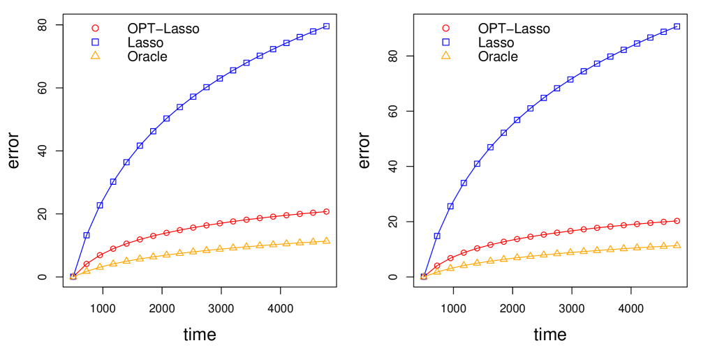
Figure 1: The $x$-axis represents time, and the $y$-axis the cumulative error from time $T/10$ to time $t\in[T/10,T]$. For scenario (c), we report the running cumulative estimation error of OPT-Lasso, Lasso and an Oracle (“LS”). The left plot corresponds to $C_{0}=0.8,C_{0}^{\textup{hard}}=0.6$ and the right plot to $C_{0}=1,C_{0}^{\textup{hard}}=0.4$.

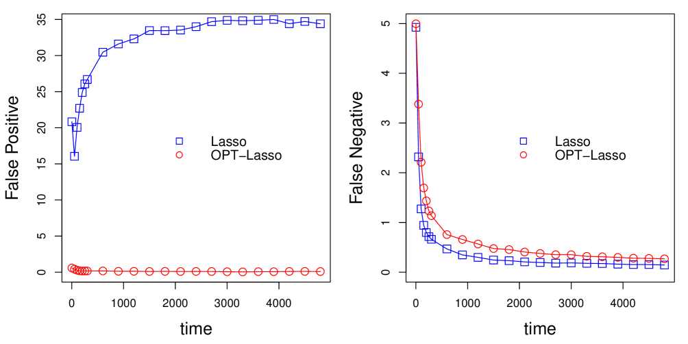
Figure 2: We consider scenario (c) and set $C_{0}=0.8,C_{0}^{\textup{hard}}=0.6$. The left (resp. right) plot shows the number of false positives (resp. negatives) at each time $t\in[T]$ for Lasso and OPT-Lasso.

3 High-dimensional Linear Contextual Bandits

In this section, we investigate the linear contextual bandit problem in high dimensions. Specifically, consider a set of $K\geq 2$ arms, each associated with an arm parameter $\boldsymbol{\theta}^{(k)}\in\mathbb{R}^{d}$. In addition, assume that there are $T$ rounds, and at each round/time $t\in[T]$, we observe a covariate vector $\boldsymbol{X}_{t}\in\mathbb{R}^{d}$, select an arm $A_{t}\in[K]$, and receive a reward $Y_{t}\in\mathbb{R}$, which satisfies the following linear model:

$$Y_{t}=\boldsymbol{X}_{t}^{\prime}\boldsymbol{\theta}^{(A_{t})}+\epsilon_{t}.$$

We assume that the covariate vectors $\{\boldsymbol{X}_{t}:t\in[T]\}$ are i.i.d., and that $\{\epsilon_{t}\in\mathbb{R}:t\in[T]\}$ are zero-mean i.i.d. random variables that are $\sigma$-sub-Gaussian, i.e., $\mathbb{E}[\exp(\tau\epsilon_{1})]\leq\exp(\sigma^{2}\tau^{2}/2)$ for $\tau\in\mathbb{R}$. Further, these two sequences are independent. At each round $t\in[T]$, we can select the arm $A_{t}$ based solely on $\boldsymbol{X}_{t}$ and the previous observations $\{(\boldsymbol{X}_{s},A_{s},Y_{s}):s<t\}$, possibly with the help of a random variable $U_{t}$. Specifically, a permissible rule $\{\pi_{t}:t\in[T]\}$ is a sequence of measurable functions such that

$$A_{t}=\pi_{t}\left(\boldsymbol{X}_{t},\{(\boldsymbol{X}_{s},A_{s},Y_{s}):s<t\},U_{t}\right),\;\text{ for }t\in[T],$$

where $\{U_{t}:t\in[T]\}$ are i.i.d. random variables uniformly distributed on $(0,1)$ and independent of all other random variables. Let $\mathcal{F}_{t}:=\sigma(\{(\boldsymbol{X}_{s},A_{s},Y_{s}),s\leq t\})$ be the $\sigma$-algebra generated by the observations up to time $t\geq 0$.

Given a permissible rule $\{\pi_{t}:t\in[T]\}$, or equivalently the arm selections $\{A_{t}:t\in[T]\}$, we define the instantaneous regret $r_{t}$ at time $t\in[T]$ as follows:

$$r_{t}:=\boldsymbol{X}_{t}^{\prime}\left(\boldsymbol{\theta}^{(A_{t}^{*})}-\boldsymbol{\theta}^{(A_{t})}\right),\;\;\text{ where }\;A_{t}^{*}:=\operatorname*{argmax}_{k\in[K]}\boldsymbol{X}_{t}^{\prime}\boldsymbol{\theta}^{(k)}.$$ (7)

Our goal is to find a procedure that minimizes the expected cumulative regret $\sum_{t\in[T]}\mathbb{E}[r_{t}]$.

We focus on the high-dimensional regime, where the time horizon $T$ may exceed the dimension $d$, but the arm parameters are assumed to be sparse. Specifically, for each arm $k\in[K]$, let $S_{k}=\{j\in[d]:\boldsymbol{\theta}^{(k)}_{j}\neq 0\}$ denote the support of $\boldsymbol{\theta}^{(k)}$, and define $s_{0}:=\max_{k\in[K]}|S_{k}|$ as the maximum support size across all arms. We consider the setting where $s_{0}\ll d$. Throughout, we assume $s_{0},d,T\geq 2$.

3.1 A Three-Stage Algorithm

We propose a three-stage algorithm that separates exploration and exploitation, as depicted in Figure 3 and described in detail below.

Figure 3: An illustration of the three-stage algorithm. The three stages are as follows: a pure exploration stage $(0,\gamma_{1}]$ with random arm selection; an exploitation stage $(\gamma_{1},\gamma_{2}]$ based on Lasso estimators; and a final exploitation stage $(\gamma_{2},T]$ based on OPT-Lasso estimators. During Stages 2 and 3, the estimators are updated every $g_{1}$ and $g_{2}$ rounds, respectively.

For round $t\in[1,\gamma_{1}]$, where $\gamma_{1}$ is to be specified, due to data scarcity, we perform pure exploration by randomly selecting one of the $K$ arms. Afterwards, we estimate the parameter of each arm and select the arm that maximizes the estimated reward, i.e., by pure exploitation. For the exploitation period, we divide it into two segments. For round $t\in(\gamma_{1},\gamma_{2}]$, where $\gamma_{2}$ is to be specified, we adopt Lasso as the estimation method, while for round $t\in(\gamma_{2},T]$, we use OPT-Lasso. For computational efficiency, we do not update the Lasso (resp. OPT-Lasso) estimator at each round, but rather every $g_{1}$ (resp. $g_{2}$) rounds, where $g_{1}$ and $g_{2}$ are tuning parameters.

Specifically, for each time $t\in[T]$ and arm $k\in[K]$, we define

$$\boldsymbol{X}_{[t]}^{(k)}=\left(\boldsymbol{X}_{1}\mathbb{I}\{A_{1}=k\},\;\cdots\;,\boldsymbol{X}_{t}\mathbb{I}\{A_{t}=k\}\right)^{\prime},$$

$$\boldsymbol{Y}_{[t]}^{(k)}=\left(Y_{1}\mathbb{I}\{A_{1}=k\},\;\cdots\;,Y_{t}\mathbb{I}\{A_{t}=k\}\right)^{\prime},$$

where $(\boldsymbol{X}_{[t]}^{(k)},\boldsymbol{Y}_{[t]}^{(k)})$ represents the data available for estimating $\boldsymbol{\theta}^{(k)}$ up to time $t$. Furthermore, for each $t\in[T]$ and $k\in[K]$, given a regularization parameter $\lambda_{t}^{(k)}$ and a hard-threshold parameter $\lambda_{t}^{\textup{OPT},(k)}$, we denote by

$$\widehat{\boldsymbol{\theta}}_{t}^{(k)}=\widehat{\boldsymbol{\theta}}^{\textup{Lasso}}_{t}\left(\boldsymbol{X}_{[t]}^{(k)},\boldsymbol{Y}_{[t]}^{(k)},\lambda_{t}^{(k)}\right),\quad\widetilde{\boldsymbol{\theta}}_{t}^{(k)}=\widehat{\boldsymbol{\theta}}^{\textup{OPT}}_{t}\left(\boldsymbol{X}_{[t]}^{(k)},\boldsymbol{Y}_{[t]}^{(k)},\lambda_{t}^{(k)},\lambda_{t}^{\textup{OPT},(k)}\right),$$

the Lasso and OPT-Lasso estimators, respectively, of the $k$-th arm parameter $\boldsymbol{\theta}^{(k)}$, where we recall their definitions in Definition 1 and 2. In general, $\lambda_{t}^{(k)}$ and $\lambda_{t}^{\textup{OPT},(k)}$ can depend on the data up to time $t$, that is, $\mathcal{F}_{t}$-measurable.

Definition 3.

Given positive integers $\gamma_{1},\gamma_{2},g_{1},g_{2}$ such that $\gamma_{1}\leq\gamma_{2}$, and parameters $\{\lambda_{t}^{(k)},\lambda_{t}^{\textup{OPT},(k)}:t\in[T],k\in[K]\}$, we formally define the three-stage algorithm as follows:

1. (Random selection). At round $t\in[1,\gamma_{1}]$, $A_{t}$ is randomly selected from $[K]$ according to a uniform distribution;

2. (Lasso). At round $t\in(\gamma_{1}+mg_{1},(\gamma_{1}+(m+1)g_{1})\wedge\gamma_{2}]$ with $m\in\{0,1,2,\cdots\}$, we use the Lasso estimators at time $\gamma_{1}+mg_{1}$, and select the arm greedily:

   $$A_{t}=\text{argmax}_{k\in[K]}(\widehat{\boldsymbol{\theta}}_{\gamma_{1}+mg_{1}}^{(k)})^{\prime}\boldsymbol{X}_{t}.$$

3. (OPT-Lasso). At round $t\in(\gamma_{2}+mg_{2},(\gamma_{2}+(m+1)g_{2})\wedge T]$ with $m\in\{0,1,2,\cdots\}$, we use the OPT-Lasso estimators at time $\gamma_{2}+mg_{2}$, and select the arm greedily:

   $$A_{t}=\text{argmax}_{k\in[K]}(\widetilde{\boldsymbol{\theta}}_{\gamma_{2}+mg_{2}}^{(k)})^{\prime}\boldsymbol{X}_{t}.$$

Here, ties in the “argmax” are broken either according to a fixed rule or randomly.

A few remarks are in order. First, based on the results in Section 2, OPT-Lasso is the preferred estimation method over Lasso in the sequential setting. Therefore, the durations of the first two stages should be significantly shorter than that of the third stage; that is, we choose $\gamma_{2}\ll T$. Second, the second stage is introduced primarily for technical reasons. Specifically, as we explain in Appendix D.1, the $\ell_{2}$ estimation error of the Lasso estimators can be bounded when $t=\Omega(s_{0}\log(dT))$. In contrast, our analysis of the OPT-Lasso estimators requires $t=\Omega(s_{0}^{5}\log(dT))$. To bridge this gap, we include an intermediate stage that uses Lasso before transitioning to OPT-Lasso in the third stage. In the simulation studies presented in Section 3.4, we observe that including Stage 2 leads to a slight improvement in the performance of the proposed procedure. Finally, in Stage 2 (resp. Stage 3), the estimators are updated every $g_{1}$ (resp. $g_{2}$) steps and may use arm-specific tuning parameters $\lambda_{t}^{(k)}$ (resp. $\lambda_{t}^{(k)}$ and $\lambda_{t}^{\textup{OPT},(k)}$). For simplicity and to reduce the number of free parameters in the subsequent analysis, we set

$$g_{1}=\gamma_{1},\;\;\quad g_{2}=\gamma_{2},\;\;\lambda_{t}^{(k)}=\lambda_{t}\;\text{ and }\;\lambda_{t}^{\textup{OPT},(k)}=\lambda_{t}^{\textup{OPT}}\;\text{ for }k\in[K],\;t\in[T].$$ (8)

This choice allows us to (nearly) characterize the minimax rate of the cumulative regret.

3.2 Minimax optimality of Proposed Algorithm

For the regret analysis, we first establish an upper bound on the cumulative regret of the proposed algorithm, followed by a (nearly) matching lower bound that holds for all admissible policies. These results demonstrate, in particular, that the proposed algorithm is (nearly) minimax optimal. We begin by stating our assumptions.

A Lebesgue-density function $f:\mathbb{R}^{d}\mapsto[0,\infty)$ is called log-concave if the function $\log f:\mathbb{R}^{d}\mapsto[-\infty,\infty)$ is concave. In addition, we define the following matrices: for $t\in[T]$,

$$\boldsymbol{\Sigma}:=\mathbb{E}[\boldsymbol{X}_{t}\boldsymbol{X}_{t}^{\prime}],\quad\boldsymbol{\Sigma}^{(k)}:=\mathbb{E}\left[\boldsymbol{X}_{t}\boldsymbol{X}_{t}^{\prime}\mathbbm{1}\{(\boldsymbol{\theta}^{(k)})^{\prime}\boldsymbol{X}_{t}\geq\max_{\ell\neq k}((\boldsymbol{\theta}^{(\ell)})^{\prime}\boldsymbol{X}_{t})\}\right]\text{ for }k\in[K].$$

Thus, $\boldsymbol{\Sigma}$ is the covariance matrix of the covariate vector, while $\boldsymbol{\Sigma}^{(k)}$ denotes the covariance matrix of the covariate vector on the event that the $k$-th arm is the optimal one. For a random variable $Z$, its $\psi_{2}$ norm is defined as follows: $\|Z\|_{\psi_{2}}:=\inf\{C>0:\exp((Z/C)^{2})\leq 2\}$.

Assumption 4 (Covariate vectors).

For constants $m_{X},\alpha_{X},L_{3}>1$, we assume

1. For each $t\in[T]$, the covariate vector $\boldsymbol{X}_{t}$ satisfies $\mathbb{E}[\boldsymbol{X}_{t}]=\boldsymbol{0}_{d}$, $\|\boldsymbol{X}_{t}\|_{\infty}\leq m_{X}$, and has a log-concave Lebesgue-density. Moreover, $\boldsymbol{X}_{t}$ is sub-Gaussian in the sense that for every unit vector $\boldsymbol{u}\in\mathbb{R}^{d}$ with $\|\boldsymbol{u}\|_{2}=1$, we have $\|\boldsymbol{u}^{\prime}\boldsymbol{X}_{t}\|_{\psi_{2}}\leq\alpha_{X}$.

2. The eigenvalues of $\boldsymbol{\Sigma}$ satisfy $L_{3}^{-1}\leq\lambda_{\min}\left(\boldsymbol{\Sigma}\right)\leq\lambda_{\max}\left(\boldsymbol{\Sigma}\right)\leq L_{3}$.

3. The covariance matrix for each arm $k\in[K]$ satisfies $|\kern-1.07639pt|\kern-1.07639pt|(\boldsymbol{\Sigma}^{(k)})^{-1}|\kern-1.07639pt|\kern-1.07639pt|_{\infty}\leq L_{3}$.

For Assumption 4 (a), it is common to assume that the entries of the covariate vectors are bounded; see, e.g., [7, 3]. Examples of distributions that are bounded, sub-Gaussian, and possess log-concave densities include the truncated normal distributions and the uniform distribution over a convex and compact set in $\mathbb{R}^{d}$.

When the covariate vector $\boldsymbol{X}_{t}$ has a log-concave density and bounded eigenvalues as assumed in Assumption 4 (b), we highlight the following two properties. First, if arms are selected to maximize the estimated rewards, then the conditional regret $\mathbb{E}[r_{t}\mid\mathcal{F}_{t-1}]$ at time $t\in[T]$ is, up to a constant depending only on $L_{3}$, both upper and lower bounded by the mean-squared estimation error of the arm parameters at time $t-1$; see Lemma 33 in Appendix. Second, for any unit vector $\boldsymbol{u}\in\mathbb{R}^{d}$, the random variable $\boldsymbol{u}^{\prime}\boldsymbol{X}_{t}$ has a density bounded by a constant $C$ depending only on $L_{3}$; see Lemma 35 in Appendix. This implies that for any $i\neq j\in[K]$, the probability that $\boldsymbol{X}_{t}$ falls within a $\tau$-distance of the boundary $\{\boldsymbol{x}\in\mathbb{R}^{d}:(\boldsymbol{\theta}^{(i)})^{\prime}\boldsymbol{x}=(\boldsymbol{\theta}^{(j)})^{\prime}\boldsymbol{x}\}$ is at most $C\tau$ for any $\tau>0$, a condition known as the margin condition [16, 7]. Additional properties are summarized in Appendix F.

Similar to Assumption 1 (d) imposed in the sequential estimation problem, Assumption 4 (c) is used to derive instance-specific upper bounds on the $\ell_{2}$ estimation error of the OPT-Lasso estimators for $\{\boldsymbol{\theta}^{(k)}:k\in[K]\}$. For example, if $K=2$ and $\boldsymbol{X}_{t}$ has a symmetric distribution, then $\boldsymbol{\Sigma}_{1}=\boldsymbol{\Sigma}_{2}=\boldsymbol{\Sigma}/2$. In this case, Assumption 4 (c) holds if $|\kern-1.07639pt|\kern-1.07639pt|(\boldsymbol{\Sigma})^{-1}|\kern-1.07639pt|\kern-1.07639pt|_{\infty}\leq L_{3}/2$.

Next, we state the assumptions on the arm parameters. For a vector $\boldsymbol{v}\in\mathbb{R}^{d}$ and a linear subspace $\mathcal{S}\subseteq\mathbb{R}^{d}$, let $\textup{proj}(\boldsymbol{v};\;\mathcal{S})$ denote the projection of $\boldsymbol{v}$ onto $\mathcal{S}$. Additionally, for a collection of vectors $\{\boldsymbol{v}_{1},\ldots,\boldsymbol{v}_{\ell}\}\subseteq\mathbb{R}^{d}$, let $\textup{span}(\boldsymbol{v}_{1},\ldots,\boldsymbol{v}_{\ell})$ denote the linear subspace spanned by this collection. We adopt the convention that the span of an empty set is $\{\boldsymbol{0}_{d}\}$.

Assumption 5 (Arm Parameters).

For constants $m_{\theta}>1$ and $L_{4}>1$, we assume

1. $\|\boldsymbol{\theta}^{(k)}\|_{2}\leq m_{\theta}$ for all $k\in[K]$.

2. Let $\boldsymbol{u}_{i,j}:=\boldsymbol{\theta}^{(i)}-\boldsymbol{\theta}^{(j)}$ for $i,j\in[K]$. Assume that for arms $k,\ell\in[K]$ with $k\neq\ell$,

   $$\|\boldsymbol{u}_{k,\ell}-\textup{proj}(\boldsymbol{u}_{k,\ell};\;\textup{span}\left(\{\boldsymbol{u}_{k,j}:j\neq k,\ell\}\right)\|_{2}\geq L_{4}^{-1}.$$

Intuitively, Assumption 5 (b) requires that the arm parameters are well-separated and linearly independent. When $K=2$, Assumption 5 (b) is equivalent to requiring $\|\boldsymbol{\theta}^{(1)}-\boldsymbol{\theta}^{(2)}\|_{2}\geq L_{4}^{-1}$. For $K\geq 2$, Assumption 5 (b) implies that $\|\boldsymbol{\theta}^{(k)}-\boldsymbol{\theta}^{(\ell)}\|_{2}\geq L_{4}^{-1}$ for $k\neq\ell\in[K]$.

Note that by definition, for $k\neq\ell\in[K]$, we have

$$\|\boldsymbol{u}_{k,\ell}-\textup{proj}(\boldsymbol{u}_{k,\ell};\textup{span}(\{\boldsymbol{u}_{k,j}:j\neq k,\ell\})\|_{2}\geq\|\boldsymbol{\theta}^{(\ell)}-\textup{proj}(\boldsymbol{\theta}^{(\ell)};\;\textup{span}(\{\boldsymbol{\theta}^{(j)}:j\neq l\}))\|_{2}.$$

Therefore, a sufficient and more interpretable condition for Assumption 5 (b) is that, for each arm $k\in[K]$, $\|\boldsymbol{\theta}^{(k)}-\textup{proj}(\boldsymbol{\theta}^{(k)};\;\textup{span}(\{\boldsymbol{\theta}^{(j)}:j\neq k\}))\|_{2}\geq L_{4}^{-1}$.

Next, we provide an upper bound on the cumulative regret of the proposed three-stage algorithm defined in Definition 3. For simplicity, we assume that the parameter choices in (8) hold, and recall that the instantaneous regret $r_{t}$ is defined in (7).

Theorem 6.

Suppose Assumptions 4 and 5 hold, and consider the proposed three-stage algorithm in Definition 3. Set the regularization and threshold parameters as

$$\lambda_{t}=6m_{X}\sigma\sqrt{\frac{\log(dT)}{t}},\quad\text{ and }\quad\lambda^{\textup{OPT}}_{t}=28L_{3}\lambda_{t},$$ (9)

and for some integers $C_{\gamma_{1}}$ and $C_{\gamma_{2}}$, set the end times of Stage 1 and 2, respectively, as follows

$$\gamma_{1}=C_{\gamma_{1}}\lceil(\sigma^{2}\vee 1)\rceil s_{0}\lceil\log(dT)\rceil,\quad\text{ and }\quad\gamma_{2}=C_{\gamma_{2}}s_{0}^{4}\gamma_{1}.$$ (10)

Then, there exist constants $C,C^{*}>0$ depending only on $K,m_{X},\alpha_{X},L_{3},m_{\theta},L_{4}$, such that if $C_{\gamma_{1}}\geq C^{*}$ and $C_{\gamma_{2}}\geq C^{*}$, then

$$\mathbb{E}\left[\sum_{t=1}^{T}r_{t}\right]\leq CC_{\gamma_{1}}(\sigma^{2}\vee 1)(\log s_{0})s_{0}(\log d+\log T).$$

Further, the following upper bound on the cumulative regret in Stage 3 holds:

$$\mathbb{E}\left[\sum_{t=\gamma_{2}+1}^{T}r_{t}\right]\leq C(\sigma^{2}\vee 1)s_{0}(\log d+\log T).$$

Proof.

The proof is provided in Section 3.5. ∎

Under the same problem formulation, [7] proposes the Lasso bandit algorithm, and provides an upper bound on the expected regret of order $O(s_{0}^{2}(\log d+\log T)^{2})$, which has worse dependence on $s_{0},d,T$ compared to the upper bound established above. As we demonstrate in Subsection 3.4, algorithms based on Lasso estimators are provably suboptimal.

Furthermore, [3] proposes a related algorithm called the “thresholded Lasso bandit”, which does not have the pure exploration stage—that is, it does not include Stage 1—and applies thresholding twice to the initial Lasso estimators. For the analysis, they assume that $s_{0}$ is constant and that the nonzero components of the parameter vectors are bounded away from zero by a constant, that is,

$$\text{(i) }s_{0}\text{ is constant,}\quad\text{and}\quad\text{(ii) }\min_{j\in S_{k},\;k\in[K]}|\boldsymbol{\theta}^{(k)}_{j}|=\Omega(1).$$ (11)

See Assumption 3.1 in [3]. Under this restrictive assumption, [3] establishes an upper bound on the cumulative regret of order $O((\log\log d)\log d+\log T)$ (see Theorem 5.2 therein). Under Assumption (11), our result in Theorem 6 provides a mild improvement by a factor of $\log\log d$ on the dependence of $d$. Importantly, our analysis allows $s_{0}$ to grow with $d$ and $T$, and does not require the beta-min condition. Moreover, if the beta-min condition is imposed, we are unable to establish a matching lower bound as in Corollary 8—that is, the minimax rate under this assumption remains unclear.

Finally, we show that the algorithm is nearly minimax optimal with respect to $s_{0},d,T$, by establishing a nearly matching lower bound of the cumulative regret under the case $K=2$. We define the following space of parameters for $\boldsymbol{\theta}^{(1)}$ and $\boldsymbol{\theta}^{(2)}$: for $L>0$,

$$\begin{split}\widetilde{\boldsymbol{\Theta}}_{d}(s_{0},L):=&\left\{(\boldsymbol{\theta}^{(1)},\boldsymbol{\theta}^{(2)})\in\mathbb{R}^{d+d}:\;\;\|\boldsymbol{\theta}^{(1)}\|_{0}\leq s_{0},\;\;\|\boldsymbol{\theta}^{(2)}\|_{0}\leq s_{0},\;\;\right.\\ &\left.\qquad\qquad\|\boldsymbol{\theta}^{(1)}\|_{2}\leq 2L,\;\;\|\boldsymbol{\theta}^{(2)}\|_{2}\leq 2L,\;\;\|\boldsymbol{\theta}^{(1)}-\boldsymbol{\theta}^{(2)}\|_{2}\geq L^{-1}\right\}.\end{split}$$

As $L$ increases, $\widetilde{\boldsymbol{\Theta}}_{d}(s_{0},L)$ becomes larger. Further, as $L\uparrow\infty$, $\widetilde{\boldsymbol{\Theta}}_{d}(s_{0},L)$ exhausts all possible pairs of $s_{0}$-sparse vectors in $\mathbb{R}^{d}$.

Theorem 7.

Consider the case $K=2$, and let $L>1$ and $C_{*}>0$ be arbitrary fixed constants. Suppose that Assumptions 4 (a) and 4 (b) hold for $\{\boldsymbol{X}_{t}:t\in[T]\}$, and that the noise $\{\epsilon_{t}:t\in[T]\}$ are $i.i.d.$ normal random variables with distribution $\mathcal{N}(0,\sigma^{2})$. Further, assume that for some constant $\kappa>1$, we have

$$3\leq s_{0}\leq(d+2)/3,\quad d\geq s_{0}^{\kappa},\quad T\geq\left(2(C_{*}\vee\sigma^{2}\vee 1)s_{0}^{5}\log(dT)\right)^{\kappa}.$$ (12)

Then there exists a constant $C>0$ depending only on $L_{3}$ and $L$, such that for any permissible rule, the following lower bound on its worst-case cumulative regret over $\widetilde{\boldsymbol{\Theta}}_{d}(s_{0},L)$, starting from time $\tilde{\gamma}:=\left\lfloor C_{*}s_{0}^{5}\log(dT)\right\rfloor$ holds:

$$\sup_{(\boldsymbol{\theta}^{(1)},\boldsymbol{\theta}^{(2)})\in\widetilde{\boldsymbol{\Theta}}_{d}(s_{0},L)}\mathbb{E}_{\boldsymbol{\theta}^{(1)},\boldsymbol{\theta}^{(2)}}\left[\sum_{t=\tilde{\gamma}}^{T}r_{t}\right]\geq C^{-1}\sigma^{2}(1-1/\kappa)s_{0}\left(\log d+\log T\right),$$

where the expectation $\mathbb{E}_{\boldsymbol{\theta}^{(1)},\boldsymbol{\theta}^{(2)}}$ is taken under the true parameter values $\boldsymbol{\theta}^{(1)}$ and $\boldsymbol{\theta}^{(2)}$.

Proof.

The proof is provided in Appendix E.1. ∎

Remark 5.

The key argument is as follows: since the context vectors have a log-concave density with bounded eigenvalues, the conditional expected instantaneous regret $\mathbb{E}[r_{t}|\mathcal{F}_{t-1}]$ can be lower bounded by the best possible mean-squared estimation errors of the arm parameters $\boldsymbol{\theta}^{(1)}$ and $\boldsymbol{\theta}^{(2)}$ at time $t-1$, using Lemma 33 in Appendix. The remainder of the argument then follows similarly to the proof of Theorem 3.

Note that a lower bound on the cumulative regret computed from time $\tilde{\gamma}$ also serves as a lower bound on the cumulative regret computed from the beginning (i.e., from time $1$). Similarly, a lower bound for a larger $L$ also applies to any smaller $L$. Combining Theorem 6 with Theorem 7, we immediately obtain the following corollary.

Corollary 8.

Consider the case $K=2$ and let $L,\kappa>1$ be fixed constants. Suppose that Assumption 4 holds, and that the noise $\{\epsilon_{t}:t\in[T]\}$ are $i.i.d.$ normal random variables with distribution $\mathcal{N}(0,\sigma^{2})$. Then there exist constants $C^{*},C>0$ depending only on $m_{X},\alpha_{X},L_{3},L$, such that if condition (12) holds with $\kappa$ and $C^{*}$ in place of $C_{*}$, then

$$C^{-1}(1-1/\kappa)\sigma^{2}\leq\frac{\inf_{\{\pi_{t}\}}\sup_{(\boldsymbol{\theta}^{(1)},\boldsymbol{\theta}^{(2)})\in\widetilde{\boldsymbol{\Theta}}_{d}(s_{0},L)}\mathbb{E}_{\boldsymbol{\theta}^{(1)},\boldsymbol{\theta}^{(2)}}\sum_{t=1}^{T}r_{t}}{s_{0}\left(\log d+\log T\right)}\leq C(\sigma^{2}\vee 1)\log(s_{0}),$$

where the infimum is taken over all permissible rules $\{\pi_{t}:t\in[T]\}$. Further, if the cumulative regret is computed starting from time $\tilde{\gamma}:=\lfloor C^{*}s_{0}^{5}\log(dT)\rfloor$, then

$$C^{-1}(1-1/\kappa)\sigma^{2}\leq\frac{\inf_{\{\pi_{t}\}}\sup_{(\boldsymbol{\theta}^{(1)},\boldsymbol{\theta}^{(2)})\in\widetilde{\boldsymbol{\Theta}}_{d}(s_{0},L)}\mathbb{E}_{\boldsymbol{\theta}^{(1)},\boldsymbol{\theta}^{(2)}}\sum_{t=\tilde{\gamma}}^{T}r_{t}}{s_{0}\left(\log d+\log T\right)}\leq C(\sigma^{2}\vee 1).$$

Proof.

The lower bound is established in Theorem 7, while the upper bound is from Theorem 6, which concerns the regret analysis of the proposed procedure. Note that $K=2$ is fixed, and for $(\boldsymbol{\theta}^{(1)},\boldsymbol{\theta}^{(2)})\in\widetilde{\boldsymbol{\Theta}}_{d}(s_{0},L)$, Assumption 5 holds with $m_{\theta}=2L$ and $L_{4}=L$. ∎

Corollary 8 characterizes the minimax rate of the overall cumulative regret up to a $\log(s_{0})$ factor, with optimal dependence on $d$ and $T$. By Theorem 6, the proposed procedure achieves this rate up to a $\log(s_{0})$ factor and is therefore minimax optimal when $s_{0}$ is constant.

The extra $\log(s_{0})$ factor in the upper bound arises from Stage 2 of the proposed algorithm, where Lasso estimators are applied to bridge the gap between the pure exploration phase and Stage 3, in which OPT-Lasso is used. Indeed, if the cumulative regret is computed starting from time $C^{*}s_{0}^{5}\log(dT)$, for some sufficiently large constant $C^{*}$, thereby ignoring the short initial period, then Corollary 8 implies that the minimax rate is exactly of order $s_{0}(\log d+\log T)$, and the proposed procedure is minimax optimal.

3.3 Suboptimality of Lasso in the Bandit Setting

In this subsection, we analyze the proposed algorithm without Stage 3 (see also Figure 3). Specifically, by setting the end time $\gamma_{2}$ of Stage 2 to $T$ in Definition 3, the algorithm reduces to two stages. After the initial exploration phase from time $1$ to $\gamma_{1}$, we employ Lasso estimators to estimate the arm parameters and select arms greedily by maximizing the estimated rewards. The goal is to demonstrate the suboptimality of Lasso in the bandit setting.

For simplicity, we assume that condition (8) holds for $g_{1}$ and $\lambda_{t}^{(k)}$. We start with an upper bound on the cumulative regret.

Corollary 9.

Suppose Assumptions 4 and 5 hold. Let $\gamma_{2}=T$ in Definition 3, that is, without Stage 3. Set the regularization parameter $\lambda_{t}$ and the end time $\gamma_{1}$ of Stage 1 as in (9) and (10), respectively. There exist constants $C,C^{*}>0$ depending only on $K,m_{X},\alpha_{X},L_{3},m_{\theta},L_{4}$, such that if the integer constant $C_{\gamma_{1}}$ in (10) satisfies $C_{\gamma_{1}}\geq C^{*}$, then

$$\mathbb{E}\left[\sum_{t=1}^{T}r_{t}\right]\leq CC_{\gamma_{1}}(\sigma^{2}\vee 1)s_{0}(\log d+\log T)\log(T).$$

Proof.

This is implied by the proof of Theorem 6; see Subsection 3.5. ∎

Compared with the minimax rate in Corollary 8, the above upper bound includes an additional $\log T$ factor. The following theorem shows that this bound is generally tight, implying that the use of standard Lasso estimators–—rather than OPT-Lasso—–is suboptimal in the bandit setting. Denote by $\mathbb{I}_{d\times d}$ the $d$-by-$d$ identity matrix.

Theorem 10.

Consider the case $K=2$ and set $\gamma_{2}=T$ in Definition 3, that is, without Stage 3. Suppose that Assumption 4 (a) holds and that $\boldsymbol{\Sigma}^{(1)}=\boldsymbol{\Sigma}^{(2)}=2^{-1}\mathbb{I}_{d\times d}$. Set the regularization parameter $\lambda_{t}$ and the end time $\gamma_{1}$ of Stage 1 as follows:

$$\gamma_{1}=C_{\gamma_{1}}\lceil(\sigma^{2}\vee 1)\rceil s_{0}\lceil\log(dT)\rceil,\quad\lambda_{t}=48m_{X}\sigma\sqrt{\frac{\log(dT)}{t}}.$$

Let $\kappa>1$ be a constant. There exist constants $C^{*},C>0$ depending only on $m_{X}$ such that if $C_{\gamma_{1}}\geq C^{*}$ and $T\geq(2C_{\gamma_{1}}C^{*}s_{0}^{5}\log(dT))^{\kappa}$, then we have the following lower bound on the worst-case cumulative regret over $\widetilde{\boldsymbol{\Theta}}_{d}(s_{0},L)$, excluding an initial period:

$$\sup_{(\boldsymbol{\theta}^{(1)},\boldsymbol{\theta}^{(2)})\in\widetilde{\boldsymbol{\Theta}}_{d}(s_{0},L)}\mathbb{E}_{\boldsymbol{\theta}^{(1)},\boldsymbol{\theta}^{(2)}}\left[\sum_{t=C_{*}C_{\gamma_{1}}s_{0}^{5}\log(dT)}^{T}r_{t}\right]\geq C^{-1}\sigma^{2}(1-1/\kappa)\log(T)(\log d+\log T).$$

Proof.

See Appendix E.2. ∎

Remark 6.

As previously discussed, a lower bound over fewer rounds immediately implies a lower bound on the overall regret.

In Theorem 10, we assume $\boldsymbol{\Sigma}^{(1)}=\boldsymbol{\Sigma}^{(2)}=2^{-1}\mathbb{I}_{d\times d}$. As discussed following Assumption 4, this condition is satisfied by many examples. Under the assumptions of Theorem 10, Corollary 8 implies that the minimax rate for cumulative regret over the same time horizon is of order $s_{0}(\log d+\log T)$. In contrast, the lower bound in Theorem 10 includes an additional $\log T$ factor. This indicates that when using Lasso estimators for pure exploitation, the resulting algorithm is minimax suboptimal in terms of both $d$ and $T$, in general. We also note that, due to technical challenges, the lower bound does not capture the explicit dependence on $s_{0}$.

3.4 Simulation Study in the Bandit Setting

In this section, we conduct simulations to compare the empirical performance of the proposed procedure in Definition 3 (denoted as “Three-stage”) with the following alternatives: (i) the Lasso bandit algorithm [7]; (ii) the procedure in Definition 3 with $\gamma_{2}=\gamma_{1}$, i.e., an algorithm that uses only OPT-Lasso estimators (denoted as “Two-stage with OPT”); (iii) the procedure in Definition 3 with $\gamma_{2}=T$, i.e., an algorithm that uses only Lasso estimators (denoted as “Two-stage with Lasso”).

We fix the time horizon to $T=10000$ and consider eight scenarios with varying sparsity $s_{0}$, dimension $d$, and number of arms $K$. The scenarios for $(s_{0},d,K)$ are: (a) $(5,100,5)$, (b) $(5,100,10)$, (c) $(10,500,5)$, (d) $(10,500,10)$, (e) $(5,1000,5)$, (f) $(5,1000,10)$, (g) $(10,1000,5)$, and (h) $(10,1000,10)$. In each scenario, for each arm $k\in[K]$, we first randomly select a subset $S_{k}$ of $s_{0}$ covariates. Then, for each $j\notin S_{k}$, we set $\boldsymbol{\theta}^{(k)}_{j}=0$, and for each $j\in S_{k}$, we sample $\boldsymbol{\theta}^{(k)}_{j}$ independently from the uniform distribution on $[0,1]$. Next, at each time $t\in[T]$, the covariate vector $\boldsymbol{X}_{t}$ is independently drawn from the standard $d$-dimensional normal distribution $\mathcal{N}(\mathbf{0}_{d},\mathbb{I}_{d\times d})$, with entries truncated to lie within $[-1,1]$; that is, for each $j\in[d]$, if $(\boldsymbol{X}_{t})_{j}>1$, we set $(\boldsymbol{X}_{t})_{j}=1$, and if $(\boldsymbol{X}_{t})_{j}<-1$, we set $(\boldsymbol{X}_{t})_{j}=-1$. Finally, at each time $t\in[T]$, the noise $\boldsymbol{\epsilon}_{t}$ is independently drawn from the standard normal distribution $\mathcal{N}(0,1)$. We perform $1000$ repetitions for each scenario.

For the proposed algorithm (“Three-stage”) and the alternative algorithms (ii) “Two-stage with OPT” and (iii) “Two-stage with Lasso,” we set the regularization and threshold parameters in Definition 3 as follows: for each $t\in[T]$ and $k\in[K]$,

$$\lambda_{t}^{(k)}=C_{0}\hat{p}_{t}^{(k)}\sqrt{{\log(d)}/{t}},\quad\lambda_{t}^{\mathrm{OPT},(k)}=C_{0}^{\mathrm{hard}}\left(C_{0}\sqrt{{\log(dt)}/{t}}\right),$$

where $\hat{p}_{t}^{(k)}:=t^{-1}\sum_{s=1}^{t}\mathbf{1}\{A_{s}=k\}$ denotes the proportion of times the $k$-th arm has been pulled up to time $t$. The end times of Stage 1 and 2 are set to $\gamma_{1}=10K$ and $\gamma_{2}=8\gamma_{1}$, respectively. Furthermore, $g_{1}$ and $g_{2}$ in Definition 3 are both set to $50$; that is, the arm parameter estimates are updated every $50$ rounds during Stages 2 and 3. Following Section 5.1 of [7], for the Lasso bandit algorithm in [7], we set $q=1$, $h=5$, and $\lambda_{1}=\lambda_{2,0}=0.025$.

Table 2 presents the cumulative regret up to time $T$ for all scenarios, where $C_{0}=2$, $C_{0}^{\textup{hard}}=0.6$ when $K=5$, and $C_{0}=2$, $C_{0}^{\textup{hard}}=1$ when $K=10$. For scenarios (e) and (f), Figure 4 shows the cumulative regret up to time $t$ for each $t\in[\gamma_{2},T]$ for the proposed three-stage algorithm and the “Two-stage with Lasso” algorithm. The remaining scenarios are presented in Appendix H. From Table 2, we observe that the proposed three-stage procedure performs favorably against the alternatives, and that the impact of $K$ is more significant than that of $s_{0}$ or $d$. The Lasso bandit algorithm exhibits significantly higher cumulative regret than the others. Furthermore, although we introduce Stage 2 with Lasso estimators (see Definition 3) for technical reasons, Table 2 shows that its inclusion slightly improves performance over the “Two-stage with OPT” algorithm. One possible explanation is that when the data is limited, as in Stage 2 under the bandit setup, Lasso outperforms OPT-Lasso. Finally, from both Table 2 and Figure 4, it is evident that using OPT-Lasso estimators in the bandit setup has much better empirical performance than using Lasso estimators. This aligns with our theoretical findings and with the observations from the sequential estimation problem in Section 2.4.

Table 2: The table shows the cumulative regret of scenarios (a)(c)(e)(g) with $C_{0}=2,C_{0}^{\textup{hard}}=0.6$ and (b)(d)(f)(h) with $C_{0}=2,C_{0}^{\textup{hard}}=1$, along with the standard deviations.

$(s_{0},d,K)$	Three-stage	Two-stage with OPT	Two-stage with Lasso	Lasso bandit
(a). $(5,100,5)$	341.4 $\pm$ 1.6	367.5 $\pm$ 2.5	376.7 $\pm$ 1.7	2109.8 $\pm$ 11.0
(b). $(5,100,10)$	869.1 $\pm$ 2.8	924.5 $\pm$ 3.3	986.2 $\pm$ 3.2	4174.8 $\pm$ 12.6
(c). $(10,500,5)$	666.0 $\pm$ 2.2	692.5 $\pm$ 2.3	724.9 $\pm$ 2.3	6584.9 $\pm$ 32.1
(d). $(10,500,10)$	1644.5 $\pm$ 4.2	1728.8 $\pm$ 4.4	1881.2 $\pm$ 4.1	12967.9 $\pm$ 40.6
(e). $(5,1000,5)$	481.6 $\pm$ 2.1	516.2 $\pm$ 2.3	559.3 $\pm$ 2.4	7356.6 $\pm$ 30.4
(f). $(5,1000,10)$	1271.4 $\pm$ 5.5	1391.4 $\pm$ 5.1	1624.8 $\pm$ 4.7	12025.5 $\pm$ 64.4
(g). $(10,1000,5)$	744.8 $\pm$ 2.5	761.4 $\pm$ 2.5	825.2 $\pm$ 2.7	9511.8 $\pm$ 46.2
(h). $(10,1000,10)$	1861.3 $\pm$ 4.7	1951.6 $\pm$ 4.9	2190.4 $\pm$ 5.3	16414.6 $\pm$ 57.7

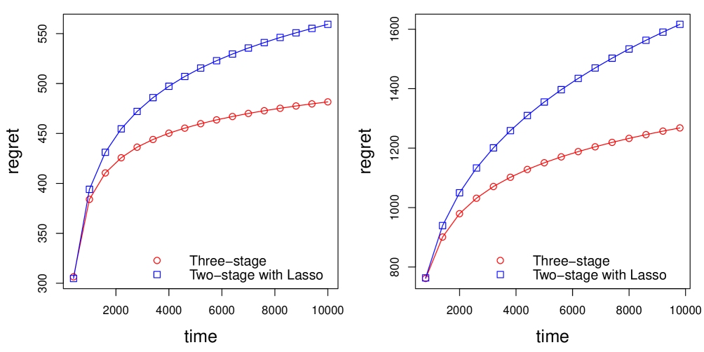
Figure 4: The $y$-axis represents the cumulative regret up to time $t\in[\gamma_{2},T]$. The left plot is for scenario (e) with $C_{0}=2,C_{0}^{\textup{hard}}=0.6,\gamma_{2}=400$, while the right plot is for scenario (f) with $C_{0}=2,C_{0}^{\textup{hard}}=1$, $\gamma_{2}=800$.

In Figure 5, we compare the support recovery performance of the OPT-Lasso and Lasso estimators under the bandit setup for scenario (e), with $C_{0}=2$ and $C_{0}^{\textup{hard}}=0.6$. Specifically, for each $t\in[T/2]$, we report the number of false positives (incorrectly selecting covariates not in the true support) and false negatives (failing to select covariates in the true support), averaged over the $K$ arms. We observe similar patterns to those in the simulation results for sequential estimation in Section 2.4; that is, the better performance of the OPT-Lasso estimator compared to Lasso is largely due to its significantly lower number of false positives.

Finally, we examine the sensitivity of the proposed three-stage algorithm to the tuning parameters $C_{0}$ and $C_{0}^{\textup{hard}}$. Table 3 shows the cumulative regret under scenarios (e) and (f); additional results are in Appendix H. The results indicate that developing principled methods for tuning parameter selection remains an important direction for future work.

Figure 5: We consider scenario (e) and (f) with $C_{0}=2,C_{0}^{\textup{hard}}=0.6$. The left plot shows the number of false positives, while the right plot shows the number of false negatives at each time $t\in[T/2]$, averaged across $K$ arms. The trend after time $T/2$ remains similar and is therefore not shown.

Table 3: Cumulative regret for scenarios (e) and (f). Bold indicates the lowest cumulative regret.

$(e)$ $C_{0}\;\backslash\;C_{0}^{\textup{hard}}$ 0.2 0.6 1.0 1.5 2 1.0 2208.7 $\pm$ 5.1 1374.5 $\pm$ 4.2 784.5 $\pm$ 2.8 557.5 $\pm$ 2.2 544.1 $\pm$ 2.1 1.6 1166.6 $\pm$ 3.8 539.5 $\pm$ 2.3 495.0 $\pm$ 3.0 599.3 $\pm$ 4.1 790.8 $\pm$ 6.3 2.0 734.1 $\pm$ 3.1 481.6 $\pm$ 2.1 561.3 $\pm$ 3.7 766.1 $\pm$ 6.3 1098.8 $\pm$ 10.8 2.6 505.8 $\pm$ 2.3 553.0 $\pm$ 2.8 761.8 $\pm$ 4.5 1226.2 $\pm$ 9.9 1873.5 $\pm$ 12.2 3.0 497.0 $\pm$ 2.3 642.7 $\pm$ 3.7 983.5 $\pm$ 7.0 1608.4 $\pm$ 10.7 2456.4 $\pm$ 15.4

$(f)$ $C_{0}\;\backslash\;C_{0}^{\textup{hard}}$ 0.2 0.6 1.0 1.5 2 1.0 4695.3 $\pm$ 8.2 4023.5 $\pm$ 7.0 2976.4 $\pm$ 5.3 1932.0 $\pm$ 4.3 1481.4 $\pm$ 3.6 1.6 3593.9 $\pm$ 7.4 2211.4 $\pm$ 5.2 1456.3 $\pm$ 5.9 1301.8 $\pm$ 5.8 1425.4 $\pm$ 7.8 2.0 2849.1 $\pm$ 5.8 1587.5 $\pm$ 4.4 1271.4 $\pm$ 5.5 1413.6 $\pm$ 7.8 1721.7 $\pm$ 11.1 2.6 1990.5 $\pm$ 5.2 1273.4 $\pm$ 4.4 1350.3 $\pm$ 5.1 1776.4 $\pm$ 9.1 2416.4 $\pm$ 14.5 3.0 1639.0 $\pm$ 4.8 1257.0 $\pm$ 4.4 1516.9 $\pm$ 7.0 2145.7 $\pm$ 12.3 3063.0 $\pm$ 19.5

3.5 Proof of Theorem 6: upper bound for the proposed procedure

In this subsection, we prove Theorem 6, which provides an upper bound on the cumulative regret of the procedure in Definition 3. A key step is bounding the $\ell_{2}$ estimation error of the Lasso estimators in Stage 2 and the OPT-Lasso estimators in Stage 3, as stated in the following theorem.

Theorem 11.

Suppose Assumptions 4 and 5 hold. Set $\lambda_{t},\lambda^{\textup{OPT}}_{t}$ as in (9), and $\gamma_{1},\gamma_{2}$ as in (10). There exist constants $C,C^{*}>0$ depending only on $K,m_{X},\alpha_{X},L_{3},m_{\theta},L_{4}$, such that if the integer constants in (10) satisfy $C_{\gamma_{1}}\geq C^{*}$ and $C_{\gamma_{2}}\geq C^{*}$, then

1. (Stage 2) For $t=m\gamma_{1}$ with $m\in\{1,2,\ldots,\gamma_{2}/\gamma_{1}\}$, we have

   $$\mathbb{P}\left(\mathcal{E}_{t}\right)\geq 1-\frac{6K}{T},\;\;\text{ where }\;\mathcal{E}_{t}:=\bigcap_{k=1}^{K}\left\{\|\widehat{\boldsymbol{\theta}}_{t}^{(k)}-\boldsymbol{\theta}^{(k)}\|_{2}^{2}\leq\frac{C\sigma^{2}s_{0}\log(dT)}{t}\right\}.$$

2. (Stage 3) For $t=m\gamma_{2}$ with $m\in\{1,2,\ldots,\lfloor T/\gamma_{2}\rfloor\}$, there exists an event $\mathcal{A}_{t}\in\mathcal{F}_{t}$ such that $\mathbb{P}(\mathcal{A}_{t})\geq 1-17K/T$, and for each arm $k\in[K]$,

   $$\mathbb{E}\left[\|\widetilde{\boldsymbol{\theta}}_{t}^{(k)}-\boldsymbol{\theta}^{(k)}\|_{2}^{2}\mathbbm{1}{\{\mathcal{A}_{t}\}}\right]\leq C\sum_{j\in S_{k}}(\boldsymbol{\theta}^{(k)}_{j})^{2}\mathbbm{1}\left\{|\boldsymbol{\theta}^{(k)}_{j}|\leq 2\lambda^{\textup{OPT}}_{t}\right\}+C\sigma^{2}s_{0}/t.$$

Part (i) of Theorem 11 follows directly from Lemma 21 in Appendix D.2, and Part (ii) is established in Lemma 23 in Appendix D.4. An overview of the proof strategy is provided in Appendix D.1, where we also elaborate on the motivation for introducing Stage 2. Note that, as with (4), the upper bound in part (ii) is instance-specific.

Given the upper bounds on the $\ell_{2}$ estimation errors, we use the assumption that the covariate vectors have a log-concave density to convert these bounds into bounds on the instantaneous regret (see Lemma 33 in Appendix). The key observation is that for $t\in[T]$, $\widehat{\boldsymbol{\theta}}_{t}^{(k)}\in\mathcal{F}_{t}$ and $\widetilde{\boldsymbol{\theta}}_{t}^{(k)}\in\mathcal{F}_{t}$ for $k\in[K]$, while $\boldsymbol{X}_{t+1}$ is independent from $\mathcal{F}_{t}$.

Proof of Theorem 6.

We choose $C^{*}>0$ as in Theorem 11. In this proof, $C$ denotes a constant, that only depends on $K,m_{X},\alpha_{X},L_{3},m_{\theta},L_{4}$ and may vary from line to line. Recall the definition of $r_{t}$ in (7).

Stage 1. Let $t\in[1,\gamma_{1}]$. By definition, $r_{t}\leq\sum_{k\in[K]}|\boldsymbol{X}_{t}^{\prime}\boldsymbol{\theta}^{(k)}|$. For each arm $k\in[K]$, due to Assumption 4 (b) and 5 (a), we have

$$\mathbb{E}\left[|\boldsymbol{X}_{t}^{\prime}\boldsymbol{\theta}^{(k)}|\right]\leq\sqrt{(\boldsymbol{\theta}^{(k)})^{\prime}\boldsymbol{\Sigma}\boldsymbol{\theta}^{(k)}}\leq m_{\theta}\sqrt{L_{3}},$$ (13)

which, together with the choice of $\gamma_{1}$ in (10), implies $\sum_{t=1}^{\gamma_{1}}\mathbb{E}[r_{t}]\leq CC_{\gamma_{1}}(\sigma^{2}\vee 1)s_{0}\log(dT)$.

Stage 2. Let $t\in(\gamma_{1},\gamma_{2}]$. For some $m\in\{1,\ldots,\gamma_{2}/\gamma_{1}\}$, we have $t\in(m\gamma_{1},(m+1)\gamma_{1}]$. Let

$$\boldsymbol{u}_{i,j}:=\boldsymbol{\theta}^{(i)}-\boldsymbol{\theta}^{(j)},\quad\hat{\boldsymbol{u}}_{i,j}:=\widehat{\boldsymbol{\theta}}^{(i)}_{m\gamma_{1}}-\widehat{\boldsymbol{\theta}}^{(j)}_{m\gamma_{1}},\quad\text{ for }i,j\in[K].$$

Due to the definition of $r_{t}$ in (7) and $A_{t}$ in Definition 3, we have

$$r_{t} =|\boldsymbol{u}_{A_{t}^{*},A_{t}}^{\prime}\boldsymbol{X}_{t}|\mathbbm{1}\{\textup{sgn}(\boldsymbol{u}_{A_{t}^{*},A_{t}}^{\prime}\boldsymbol{X}_{t})\neq\textup{sgn}(\hat{\boldsymbol{u}}_{A_{t}^{*},A_{t}}^{\prime}\boldsymbol{X}_{t})\},$$

where for $\tau\in\mathbb{R}$, $\textup{sgn}(\tau):=\mathbbm{1}\{\tau>0\}-\mathbbm{1}\{\tau<0\}$. This is because if $r_{t}=0$, both sides equal zero; while if $r_{t}>0$, then $\boldsymbol{u}_{A_{t}^{*},A_{t}}^{\prime}\boldsymbol{X}_{t}>0$ and $\hat{\boldsymbol{u}}_{A_{t}^{*},A_{t}}^{\prime}\boldsymbol{X}_{t}\leq 0$. Therefore, we have

$$r_{t}\leq\sum_{i\neq j\in[K]}|\boldsymbol{u}_{i,j}^{\prime}\boldsymbol{X}_{t}|\mathbbm{1}\{\textup{sgn}(\boldsymbol{u}_{i,j}^{\prime}\boldsymbol{X}_{t})\neq\textup{sgn}(\hat{\boldsymbol{u}}_{i,j}^{\prime}\boldsymbol{X}_{t})\}.$$

Since $\hat{\boldsymbol{u}}_{i,j}\in\mathcal{F}_{m\gamma_{1}}$ and $\boldsymbol{X}_{t}$ is independent from $\mathcal{F}_{m\gamma_{1}}$, due to Assumption 4 (a) and by applying Lemma 33 conditional on $\mathcal{F}_{m\gamma_{1}}$, we have that for $i\neq j\in[K]$, almost surely (a.s.),

$$\mathbb{E}\left[|\boldsymbol{u}_{i,j}^{\prime}\boldsymbol{X}_{t}|\mathbbm{1}\{\textup{sgn}(\boldsymbol{u}_{i,j}^{\prime}\boldsymbol{X}_{t})\neq\textup{sgn}(\hat{\boldsymbol{u}}_{i,j}^{\prime}\boldsymbol{X}_{t})\}|\mathcal{F}_{m\gamma_{1}}\right]\leq C{\|\boldsymbol{u}_{i,j}-\hat{\boldsymbol{u}}_{i,j}\|_{2}^{2}}/{\|\boldsymbol{u}_{i,j}\|_{2}}.$$

Due to Assumption 5 (b), $\|\boldsymbol{u}_{i,j}\|_{2}\geq L_{4}^{-1}$ for $i\neq j\in[K]$. By the triangle inequality, a.s.,

$$\mathbb{E}\left[r_{t}|\mathcal{F}_{m\gamma_{1}}\right]\leq C\sum_{k\in[K]}\|\widehat{\boldsymbol{\theta}}^{(k)}_{m\gamma_{1}}-\boldsymbol{\theta}^{(k)}\|_{2}^{2}.$$

Recall the event $\mathcal{E}_{m\gamma_{1}}\in\mathcal{F}_{m\gamma_{1}}$ in Theorem 11. By definition, a.s.,

$$\mathbb{E}[r_{t}\mathbbm{1}\{\mathcal{E}_{m\gamma_{1}}\}|\mathcal{F}_{m\gamma_{1}}]\leq C\sum_{k\in[K]}\|\widehat{\boldsymbol{\theta}}^{(k)}_{m\gamma_{1}}-\boldsymbol{\theta}^{(k)}\|_{2}^{2}\mathbbm{1}\{\mathcal{E}_{m\gamma_{1}}\}\leq C\sigma^{2}\frac{s_{0}\log(dT)}{m\gamma_{1}}.$$

Further, on the event $\mathcal{E}_{m\gamma_{1}}^{c}$, we use the bound: $r_{t}\leq\sum_{k\in[K]}|\boldsymbol{X}_{t}^{\prime}\boldsymbol{\theta}^{(k)}|$. Since $X_{t}$ is independent from $\mathcal{F}_{m\gamma_{1}}$, a.s.,

$$\mathbb{E}[r_{t}\mathbbm{1}\{\mathcal{E}_{m\gamma_{1}}^{c}\}|\mathcal{F}_{m\gamma_{1}}]=\sum_{k\in[K]}\mathbb{E}\left[|\boldsymbol{X}_{t}^{\prime}\boldsymbol{\theta}^{(k)}|\right]\mathbbm{1}\{\mathcal{E}_{m\gamma_{1}}^{c}\}\leq C\mathbbm{1}\{\mathcal{E}_{m\gamma_{1}}^{c}\},$$

where we use (13) in the last step. Due to Theorem 11(i) and by the law of total expectation,

$$\mathbb{E}\left[r_{t}\right]\leq C\sigma^{2}\frac{s_{0}\log(dT)}{m\gamma_{1}}+C\frac{1}{T},$$

which implies the following upper bound on the cumulative regret in Stage 2:

$$\sum_{t=\gamma_{1}+1}^{\gamma_{2}}\mathbb{E}[r_{t}]\leq C\sum_{m=1}^{\gamma_{2}/\gamma_{1}}\gamma_{1}\left(\sigma^{2}\frac{s_{0}\log(dT)}{m\gamma_{1}}+\frac{1}{T}\right)\leq C(\sigma^{2}\vee 1)\log(\gamma_{2}/\gamma_{1})s_{0}\log(dT).$$

Due to the choice of $\gamma_{1}$ and $\gamma_{2}$ in (10), $\sum_{t=\gamma_{1}+1}^{\gamma_{2}}\mathbb{E}[r_{t}]\leq C(\sigma^{2}\vee 1)\log(s_{0})s_{0}\log(dT)$.

Stage 3. Let $t\in(\gamma_{2},T]$. Then for some $m\in\{1,\ldots,\lfloor T/\gamma_{2}\rfloor\}$, we have $t\in(m\gamma_{2},(m+1)\gamma_{2}]$. Recall the event $\mathcal{A}_{m\gamma_{2}}$ in Theorem 11(ii). By similar arguments as for Stage 2,

$$\mathbb{E}[r_{t}]\leq C\sum_{k\in[K]}\left(\mathbb{E}\left[\|\widetilde{\boldsymbol{\theta}}_{m\gamma_{2}}^{(k)}-\boldsymbol{\theta}^{(k)}\|_{2}^{2}\mathbbm{1}{\{\mathcal{A}_{m\gamma_{2}}\}}\right]\right)+C\mathbb{P}(\mathcal{A}_{m\gamma_{2}}^{c}).$$

Then due to Theorem 11(ii),

$$\mathbb{E}[r_{t}]\leq C\sum_{k\in[K]}\left(\sum_{j\in S_{k}}(\boldsymbol{\theta}^{(k)}_{j})^{2}\mathbbm{1}\left\{|\boldsymbol{\theta}^{(k)}_{j}|\leq 2\lambda^{\textup{OPT}}_{m\gamma_{2}}\right\}+\frac{\sigma^{2}s_{0}}{m\gamma_{2}}\right)+\frac{C}{T}.$$

It is elementary to see that $\sum_{m=1}^{\lfloor T/\gamma_{2}\rfloor}\gamma_{2}\left(\frac{\sigma^{2}s_{0}}{m\gamma_{2}}+\frac{1}{T}\right)\leq C(\sigma^{2}\vee 1)s_{0}\log T$. Further, due to Lemma 2 and the choice of $\lambda^{\textup{OPT}}_{t}$ in (9), we have

$$\sum_{k\in[K]}\sum_{m=1}^{\lfloor T/\gamma_{2}\rfloor}\gamma_{2}\sum_{j\in S_{k}}(\boldsymbol{\theta}^{(k)}_{j})^{2}\mathbbm{1}\left\{|\boldsymbol{\theta}^{(k)}_{j}|\leq 2\lambda^{\textup{OPT}}_{m\gamma_{2}}\right\}\leq C\sigma^{2}s_{0}\log(dT).$$

Thus, $\sum_{t=\gamma_{2}+1}^{T}\mathbb{E}[r_{t}]\leq C(\sigma^{2}\vee 1)s_{0}\log(dT)$. The proof is then complete by combining the upper bounds on the cumulative regret from each stage. ∎

4 Conclusion

We study the problem of high-dimensional stochastic linear contextual bandits under sparsity constraints. To isolate the effect of estimation methods, we first analyze a related sequential estimation problem in which no arm selection is involved. We show that while the Lasso estimator is minimax optimal in the fixed-time setting, it is suboptimal in terms of cumulative estimation error in the sequential setting. In contrast, OPT-Lasso estimators attain the minimax rate in the sequential regime. Building on these insights, we propose a three-stage algorithm for the contextual bandit problem that primarily relies on OPT-Lasso estimators. We derive upper bounds on its cumulative regret and matching lower bounds over all permissible policies, thereby showing that the algorithm is nearly minimax optimal—up to a $\log(s_{0})$ factor—over the full horizon, and exactly minimax optimal if an initial short transient phase is excluded.

Several directions remain for future investigation. First, it is an open question whether the $\log s_{0}$ gap in the overall regret bound can be eliminated. Second, developing principled methods for tuning parameter selection in the proposed three-stage algorithm is of practical importance. Third, extending the framework to nonlinear models with high-dimensional covariates is an interesting direction for future research.

Appendix A Lasso and OPT-Lasso: Deterministic Analysis

In this Appendix, we consider the following deterministic linear regression model

$$\boldsymbol{Y}=\boldsymbol{Z}\boldsymbol{\theta}+\boldsymbol{\epsilon},$$

where $\boldsymbol{Z}\in\mathbb{R}^{n\times d}$ is a deterministic design matrix, $\boldsymbol{\epsilon}\in\mathbb{R}^{n}$ is a deterministic noise vector, and $\boldsymbol{\theta}=(\boldsymbol{\theta}_{1},\ldots,\boldsymbol{\theta}_{d})^{\prime}\in\mathbb{R}^{d}$ is an unknown vector. We review several well-known results for Lasso estimators and derive new results for OPT-Lasso estimators. Specifically, denote by

$$\widehat{\boldsymbol{\theta}}^{\textup{Lasso}}_{n}:=\widehat{\boldsymbol{\theta}}^{\textup{Lasso}}_{n}(\boldsymbol{Z},\boldsymbol{Y},\lambda_{n}),\quad\text{ and }\quad\widehat{\boldsymbol{\theta}}^{\textup{OPT}}_{n}:=\widehat{\boldsymbol{\theta}}^{\textup{OPT}}_{n}(\boldsymbol{Z},\boldsymbol{Y},\lambda_{n},\lambda^{\textup{OPT}}_{n})$$

the Lasso estimator (see Definition 1) and the OPT-Lasso estimator (see Definition 2) respectively, where $\lambda_{n},\lambda^{\textup{OPT}}_{n}>0$ are to be specified.

Denote by $S:=\{j\in[d]:\boldsymbol{\theta}_{j}\neq 0\}$ the support of $\boldsymbol{\theta}$ and let $s_{0}=|S|\vee 1$. Further, denote by $\hat{\boldsymbol{\Sigma}}_{n}=n^{-1}\boldsymbol{Z}^{\prime}\boldsymbol{Z}\in\mathbb{R}^{d\times d}$ the sample covariance matrix. Note that $\boldsymbol{Z}_{S}^{\prime}\boldsymbol{Z}_{S}/n=(\hat{\boldsymbol{\Sigma}}_{n})_{S,S}$.

Definition 4.

A matrix $\boldsymbol{Z}\in\mathbb{R}^{n\times d}$ is said to satisfy the restricted eigenvalue condition $\textup{RE}(s,\kappa,\rho)$ for some $s\in[d]$ and $\kappa,\rho>0$ if

$$n^{-1}\|\boldsymbol{Z}\boldsymbol{v}\|_{2}^{2}\geq\rho\|\boldsymbol{v}\|_{2}^{2},\quad\text{ for all }\boldsymbol{v}\in\mathcal{C}(s,\kappa),$$

where we define

$$\mathcal{C}(s,\kappa):=\{\boldsymbol{v}\in\mathbb{R}^{d}\backslash\{\boldsymbol{0}_{d}\}:\text{there exists }J\subseteq[d]\text{ such that }|J|=s,\text{ and }\|\boldsymbol{v}_{J^{c}}\|_{1}\leq\kappa\|\boldsymbol{v}_{J}\|_{1}\}.$$

Remark 7.

The above definition is adapted from [44, Definition 7.12].

The following $\ell_{1},\ell_{2}$, and $\ell_{\infty}$ bounds on the estimation error of the Lasso estimator $\widehat{\boldsymbol{\theta}}^{\textup{Lasso}}_{n}$ are well-known and are provided here for convenient reference.

Lemma 12.

Let $a>0$ and $\boldsymbol{A}\in\mathbb{R}^{d\times d}$ be any invertible matrix. Assume that $\boldsymbol{Z}$ satisfies the $\textup{RE}(s_{0},3,a)$ condition, and that $\lambda_{n}\geq 2\|\boldsymbol{Z}^{\prime}\boldsymbol{\epsilon}/n\|_{\infty}$. Then

$$\|\widehat{\boldsymbol{\theta}}^{\textup{Lasso}}_{n}-\boldsymbol{\theta}\|_{1}\leq{8s_{0}\lambda_{n}}/{a},$$

$$\|\widehat{\boldsymbol{\theta}}^{\textup{Lasso}}_{n}-\boldsymbol{\theta}\|_{2}\leq{3\sqrt{s_{0}}\lambda_{n}}/{a},$$

$$\|\widehat{\boldsymbol{\theta}}^{\textup{Lasso}}_{n}-\boldsymbol{\theta}\|_{\infty}\leq|\kern-1.07639pt|\kern-1.07639pt|\boldsymbol{A}^{-1}|\kern-1.07639pt|\kern-1.07639pt|_{1}\left(4+8|\kern-1.07639pt|\kern-1.07639pt|\hat{\boldsymbol{\Sigma}}_{n}-\boldsymbol{A}|\kern-1.07639pt|\kern-1.07639pt|_{\textup{max}}s_{0}/a\right)\lambda_{n}.$$

Proof.

The $\ell_{1}$ bound follows from Theorem 6.1 in [12], while the $\ell_{2}$ bound from Theorem 7.13 (a) in [45]. The $\ell_{\infty}$ bound is derived from Lemma 4.1 in [42], combined with the $\ell_{1}$ bound above. ∎

Recall the definition of $\hat{S}^{\textup{OPT}}_{n}:=\{j\in[d]:|(\widehat{\boldsymbol{\theta}}^{\textup{Lasso}}_{n})_{j}|>\lambda^{\textup{OPT}}_{n}\}$ in Definition 2. Define the following set

$$S_{n}^{\textup{str}}:=\{j\in[d]:|\boldsymbol{\theta}_{j}|>2\lambda^{\textup{OPT}}_{n}\},$$

which contains the indices of components of $\boldsymbol{\theta}$ whose magnitudes exceed $2\lambda^{\textup{OPT}}_{n}$.

Lemma 13.

If $\|\widehat{\boldsymbol{\theta}}^{\textup{Lasso}}_{n}-\boldsymbol{\theta}\|_{\infty}\leq\lambda^{\textup{OPT}}_{n}$, then $S_{n}^{\textup{str}}\subseteq\hat{S}^{\textup{OPT}}_{n}\subseteq S$.

Proof.

Let $j\in S_{n}^{\textup{str}}$ and $k\in\hat{S}^{\textup{OPT}}_{n}$. Since $\|\widehat{\boldsymbol{\theta}}^{\textup{Lasso}}_{n}-\boldsymbol{\theta}\|_{\infty}\leq\lambda^{\textup{OPT}}_{n}$, by triangle inequality and definition, we have

$$|(\widehat{\boldsymbol{\theta}}^{\textup{Lasso}}_{n})_{j}|\geq|\boldsymbol{\theta}_{j}|-\lambda^{\textup{OPT}}_{n}>\lambda^{\textup{OPT}}_{n},\qquad|\boldsymbol{\theta}_{k}|\geq|(\widehat{\boldsymbol{\theta}}^{\textup{Lasso}}_{n})_{k}|-\lambda^{\textup{OPT}}_{n}>0,$$

which implies $j\in\hat{S}^{\textup{OPT}}_{n}$ and $k\in S$. The proof is complete. ∎

Next, we provide an instance-specific upper bound on the $\ell_{2}$ estimation error of the OPT-Lasso estimator $\widehat{\boldsymbol{\theta}}^{\textup{OPT}}_{n}$.

Theorem 14.

Assume $\|\widehat{\boldsymbol{\theta}}^{\textup{Lasso}}_{n}-\boldsymbol{\theta}\|_{\infty}\leq\lambda^{\textup{OPT}}_{n}$.

1. If the support $S$ of $\boldsymbol{\theta}$ is an empty set, then $\|\widehat{\boldsymbol{\theta}}^{\textup{OPT}}_{n}-\boldsymbol{\theta}\|_{2}=0$;

2. If the support $S$ of $\boldsymbol{\theta}$ is not an empty set, assume further that for some $0<a<b$,

   $$a\leq\lambda_{\min}\left((\hat{\boldsymbol{\Sigma}}_{n})_{S,S}\right)\leq\lambda_{\max}\left((\hat{\boldsymbol{\Sigma}}_{n})_{S,S}\right)\leq b.$$

   Then we have

   $$\|\widehat{\boldsymbol{\theta}}^{\textup{OPT}}_{n}-\boldsymbol{\theta}\|_{2}^{2}\leq(2b/a+1)\sum_{j\in S}\boldsymbol{\theta}_{j}^{2}\mathbbm{1}\left\{|\boldsymbol{\theta}_{j}|\leq 2\lambda^{\textup{OPT}}_{n}\right\}+(2/a^{2})\|\boldsymbol{Z}_{S}^{\prime}\boldsymbol{\epsilon}/n\|_{2}^{2}.$$

Proof.

By Lemma 13, we have $S_{n}^{\textup{str}}\subseteq\hat{S}^{\textup{OPT}}_{n}\subseteq S$. By definition, we have

$$\left\|\widehat{\boldsymbol{\theta}}^{\textup{OPT}}_{n}-\boldsymbol{\theta}\right\|_{2}^{2}=\left\|(\widehat{\boldsymbol{\theta}}^{\textup{OPT}}_{n}-\boldsymbol{\theta})_{S}\right\|_{2}^{2}=\left\|\boldsymbol{\theta}_{S\backslash\hat{S}^{\textup{OPT}}_{n}}\right\|_{2}^{2}+\left\|(\widehat{\boldsymbol{\theta}}^{\textup{OPT}}_{n}-\boldsymbol{\theta})_{\hat{S}^{\textup{OPT}}_{n}}\right\|_{2}^{2}$$ (14)

If $S$ is an empty set, then $\widehat{\boldsymbol{\theta}}^{\textup{OPT}}_{n}=\boldsymbol{\theta}=\boldsymbol{0}_{d}$.

If $S$ is not empty and $\hat{S}^{\textup{OPT}}_{n}$ is an empty set, then $S_{n}^{\textup{str}}$ must be empty, which implies that $|\boldsymbol{\theta}_{j}|\leq 2\lambda^{\textup{OPT}}_{n}$ for all $j\in[d]$. Thus by (14), we have

$$\left\|\widehat{\boldsymbol{\theta}}^{\textup{OPT}}_{n}-\boldsymbol{\theta}\right\|_{2}^{2}=\|\boldsymbol{\theta}_{S}\|_{2}^{2}=\sum_{j\in S}\boldsymbol{\theta}_{j}^{2}\mathbbm{1}\left\{\left|\boldsymbol{\theta}_{j}\right|\leq 2\lambda^{\textup{OPT}}_{n}\right\}.$$

Now, we focus on the case that neither $S$ nor $\hat{S}^{\textup{OPT}}_{n}$ is empty, and we bound the two terms on the right-hand side of (14). For the first term in (14), by definition, we have

$$\|\boldsymbol{\theta}_{S\backslash\hat{S}^{\textup{OPT}}_{n}}\|_{2}^{2}\leq\|\boldsymbol{\theta}_{S\backslash S_{n}^{\textup{str}}}\|_{2}^{2}=\sum_{j\in S}\boldsymbol{\theta}_{j}^{2}\mathbbm{1}\left\{\left|\boldsymbol{\theta}_{j}\right|\leq 2\lambda^{\textup{OPT}}_{n}\right\}.$$ (15)

Next, we bound the second term in (14). To simplify notations, denote $\hat{S}^{\textup{OPT}}_{n}$ by $\hat{S}_{n}$. Since $\hat{S}_{n}\subseteq S$, we have

$$\lambda_{\min}\left((\hat{\boldsymbol{\Sigma}}_{n})_{\hat{S}_{n},\hat{S}_{n}}\right)\geq\lambda_{\min}\left((\hat{\boldsymbol{\Sigma}}_{n})_{S,S}\right)\geq a>0,$$

which in particular implies that $\boldsymbol{Z}_{\hat{S}_{n}}^{\prime}\boldsymbol{Z}_{\hat{S}_{n}}$ is invertible. By the definition of OPT-Lasso (see Definition 2), we have

$$(\widehat{\boldsymbol{\theta}}^{\textup{OPT}}_{n})_{\hat{S}_{n}} =\left(\boldsymbol{Z}_{\hat{S}_{n}}^{\prime}\boldsymbol{Z}_{\hat{S}_{n}}\right)^{-1}\boldsymbol{Z}_{\hat{S}_{n}}^{\prime}\boldsymbol{Y}=\left(\boldsymbol{Z}_{\hat{S}_{n}}^{\prime}\boldsymbol{Z}_{\hat{S}_{n}}\right)^{-1}\boldsymbol{Z}_{\hat{S}_{n}}^{\prime}\left(\boldsymbol{Z}_{\hat{S}_{n}}\boldsymbol{\theta}_{\hat{S}_{n}}+\boldsymbol{Z}_{S\backslash\hat{S}_{n}}\boldsymbol{\theta}_{S\backslash\hat{S}_{n}}+\boldsymbol{\epsilon}\right)$$

$$=\boldsymbol{\theta}_{\hat{S}_{n}}+\left(\boldsymbol{Z}_{\hat{S}_{n}}^{\prime}\boldsymbol{Z}_{\hat{S}_{n}}\right)^{-1}\boldsymbol{Z}_{\hat{S}_{n}}^{\prime}\left(\boldsymbol{Z}_{S\backslash\hat{S}_{n}}\boldsymbol{\theta}_{S\backslash\hat{S}_{n}}+\boldsymbol{\epsilon}\right),$$

which implies that

$$\left\|\boldsymbol{Z}_{\hat{S}_{n}}\left((\widehat{\boldsymbol{\theta}}_{n}-\boldsymbol{\theta})_{\hat{S}_{n}}\right)\right\|_{2}^{2}=\left\|\mathcal{P}_{\hat{S}_{n}}\left(\boldsymbol{Z}_{S\backslash\hat{S}_{n}}\boldsymbol{\theta}_{S\backslash\hat{S}_{n}}+\boldsymbol{\epsilon}\right)\right\|_{2}^{2},$$ (16)

where for a non-empty set $A\subseteq[S]$, we define $\mathcal{P}_{A}:=\boldsymbol{Z}_{A}\left(\boldsymbol{Z}_{A}^{\prime}\boldsymbol{Z}_{A}\right)^{-1}\boldsymbol{Z}_{A}^{\prime}$.

For the left-hand side of (16), we have

$$\begin{split}\left\|\boldsymbol{Z}_{\hat{S}_{n}}\left((\widehat{\boldsymbol{\theta}}_{n}-\boldsymbol{\theta})_{\hat{S}_{n}}\right)\right\|_{2}^{2}&\geq n\lambda_{\min}\left((\hat{\boldsymbol{\Sigma}}_{n})_{\hat{S}_{n},\hat{S}_{n}}\right)\cdot\left\|(\widehat{\boldsymbol{\theta}}^{\textup{OPT}}_{n}-\boldsymbol{\theta})_{\hat{S}_{n}}\right\|_{2}^{2}\\ &\geq na\left\|(\widehat{\boldsymbol{\theta}}^{\textup{OPT}}_{n}-\boldsymbol{\theta})_{\hat{S}_{n}}\right\|_{2}^{2}.\end{split}$$ (17)

For the right-hand side of (16), we first note that $\mathcal{P}_{A}$ is the projection matrix onto the column space of $Z_{A}$. Since $\hat{S}_{n}\subseteq S$, we have

$$\left\|\mathcal{P}_{\hat{S}_{n}}\left(\boldsymbol{Z}_{S\backslash\hat{S}_{n}}\boldsymbol{\theta}_{S\backslash\hat{S}_{n}}+\boldsymbol{\epsilon}\right)\right\|_{2}^{2}\leq 2\left\|\mathcal{P}_{\hat{S}_{n}}\boldsymbol{Z}_{S\backslash\hat{S}_{n}}\boldsymbol{\theta}_{S\backslash\hat{S}_{n}}\right\|_{2}^{2}+2\left\|\mathcal{P}_{\hat{S}_{n}}\boldsymbol{\epsilon}\right\|_{2}^{2}$$ (18)

$$\leq 2\left\|\boldsymbol{Z}_{S\backslash\hat{S}_{n}}\boldsymbol{\theta}_{S\backslash\hat{S}_{n}}\right\|_{2}^{2}+2\left\|\mathcal{P}_{S}\boldsymbol{\epsilon}\right\|_{2}^{2}$$

$$\leq 2n\lambda_{\max}\left((\hat{\boldsymbol{\Sigma}}_{n})_{S\backslash\hat{S}_{n},S\backslash\hat{S}_{n}}\right)\left\|\boldsymbol{\theta}_{S\backslash\hat{S}_{n}}\right\|_{2}^{2}+2n[\lambda_{\min}\left((\hat{\boldsymbol{\Sigma}}_{n})_{S,S}\right)]^{-1}\|\boldsymbol{Z}_{S}^{\prime}\boldsymbol{\epsilon}/n\|_{2}^{2}.$$

where the first inequality is due to the triangle inequality, the second inequality follows from the properties of projection matrices, and the final inequality follows from the definition of the eigenvalues.

Note that if $S\backslash\hat{S}_{n}$ is empty, the first term above is understood to be zero by convention. If $S\backslash\hat{S}_{n}$ is empty, we have $\lambda_{\max}\left((\hat{\boldsymbol{\Sigma}}_{n})_{S\backslash\hat{S}_{n},S\backslash\hat{S}_{n}}\right)\leq\lambda_{\max}\left((\hat{\boldsymbol{\Sigma}}_{n})_{S,S}\right)\leq b$. Therefore by (16), (17), and (18), we have

$$\left\|(\widehat{\boldsymbol{\theta}}^{\textup{OPT}}_{n}-\boldsymbol{\theta})_{\hat{S}_{n}}\right\|_{2}^{2} \leq\frac{2b}{a}\left\|\boldsymbol{\theta}_{S\backslash\hat{S}_{n}}\right\|_{2}^{2}+\frac{2}{a^{2}}\|\boldsymbol{Z}_{S}^{\prime}\boldsymbol{\epsilon}/n\|_{2}^{2}.$$

Then the proof is complete due to (15) and (14). ∎

Appendix B Lower Bounds on Bayes Risks

In this appendix, we consider the following linear model $\boldsymbol{Y}=\boldsymbol{Z}\boldsymbol{\theta}+\boldsymbol{\epsilon}$ within the Bayesian framework, where $\boldsymbol{Z}=(\boldsymbol{Z}_{1},\cdots,\boldsymbol{Z}_{n})^{\prime}\in\mathbb{R}^{n\times d}$ is a random design matrix with i.i.d. rows, $\boldsymbol{\epsilon}=(\epsilon_{1},\cdots,\epsilon_{n})^{\prime}\in\mathbb{R}^{n}$ is a noise vector with i.i.d. entries distributed as $\mathcal{N}(0,\sigma^{2})$, and $\boldsymbol{\theta}=(\boldsymbol{\theta}_{1},\cdots,\boldsymbol{\theta}_{d})\in\mathbb{R}^{d}$ is a random vector with some prior distribution to be specified.

Our goal is to derive lower bounds on the Bayes risks for estimating certain functionals of $\boldsymbol{\theta}$ based on $\boldsymbol{Y}$ and $\boldsymbol{Z}$, under two types of prior distributions on $\boldsymbol{\theta}$. Note that each estimator belongs to $\boldsymbol{\Theta}_{n,d}$, the set of all measurable functions from $\mathbb{R}^{d}\times\mathbb{R}^{n\times d}$ to $\mathbb{R}^{d}$.

Assumption 6.

For some constant $L>1$, we have $L^{-1}\leq\lambda_{\min}\left(\boldsymbol{\Sigma}\right)\leq\lambda_{\max}\left(\boldsymbol{\Sigma}\right)\leq L$.

First, we define a family of prior distributions for $\boldsymbol{\theta}$, under which the support of $\boldsymbol{\theta}$ is known. For $s\geq 2$ and $r>0$, define a probability density function (pdf) with respect to the Lebesgue measure on $\mathbb{R}^{s}$ as follows: for $\boldsymbol{u}\in\mathbb{R}^{s}$,

$$\rho_{s,r}(\boldsymbol{u}):=\frac{\tilde{\rho}_{r}(\|\boldsymbol{u}\|_{2})}{A_{s}\|\boldsymbol{u}\|_{2}^{s-1}},\quad\text{ where }\;\tilde{\rho}_{r}(\tau):=4r^{-1}\sin^{2}(2\pi r^{-1}\tau)\mathbbm{1}\{r/2\leq\tau\leq r\},$$

where $A_{s}$ is the Lebesgue area of the $s$ dimensional unit sphere $\mathcal{S}^{s-1}$.

Definition 5.

Let $2\leq s\leq d$ and $r>0$. Define $\omega_{1}(s,r)$ as the distribution of the random vector $\boldsymbol{\theta}\in\mathbb{R}^{d}$ given by the following construction: $\boldsymbol{\theta}_{j}=0$ for $j\in\{s+1,\ldots,d\}$, and $\boldsymbol{\theta}_{[s]}$ has the Lebesgue density $\rho_{s,r}$.

Lemma 15.

Let $2\leq s\leq d$ and $r>0$. Suppose that Assumption 6 holds, and that $\boldsymbol{\theta}$ has the prior distribution $\omega_{1}(s,r)$. Then, for some constant $C>0$, depending only on $r$, we have

$$\inf_{\widehat{\boldsymbol{\theta}}_{n}\in\boldsymbol{\Theta}_{n,d}}\;\mathbb{E}_{\boldsymbol{\theta}\sim\omega_{1}(s,r)}\left(\left\|\widehat{\boldsymbol{\theta}}_{n}-\boldsymbol{\theta}\right\|_{2}^{2}\right)\geq\frac{\sigma^{2}s}{C(n+\sigma^{2}s)},$$

$$\inf_{\widehat{\boldsymbol{\theta}}_{n}\in\boldsymbol{\Theta}_{n,d}}\;\mathbb{E}_{\boldsymbol{\theta}\sim\omega_{1}(s,r)}\left(\left\|\widehat{\boldsymbol{\theta}}_{n}-\frac{\boldsymbol{\theta}}{\|\boldsymbol{\theta}\|_{2}}\right\|_{2}^{2}\right)\geq\frac{\sigma^{2}s}{C(n+\sigma^{2}s)}.$$

Proof.

Under the prior distribution $\omega_{1}(s,r)$, $\boldsymbol{\theta}$ is supported on $[s]$ with probability $1$, which implies the same property holds for the posterior means: $\mathbb{E}[\boldsymbol{\theta}|Y,Z]$ and $\mathbb{E}[\boldsymbol{\theta}/\|\boldsymbol{\theta}\|_{2}\;|Y,Z]$. Then, the results follow from Theorem 31 in [36]. ∎

Next, we define the second family of prior distributions for $\boldsymbol{\theta}\in\mathbb{R}^{d}$, which is supported on finitely many $\mathbb{R}^{d}$ vectors. We begin with a lemma.

Lemma 16.

Let $3\leq s\leq d$ and $r,\delta>0$. There exists $M\in\mathbb{N}$ and vectors $\boldsymbol{\alpha}_{1},\cdots,\boldsymbol{\alpha}_{M}\in\mathbb{R}^{d}$ such that for any indexes $i\neq j\in[M]$, we have

$$\left\|\boldsymbol{\alpha}_{i}\right\|_{0}=s,\quad\|\boldsymbol{\alpha}_{i}\|_{2}^{2}=r^{2}+2\delta^{2},\quad\delta^{2}\leq\|\boldsymbol{\alpha}_{i}-\boldsymbol{\alpha}_{j}\|_{2}^{2}\leq 8\delta^{2},\quad\log M\geq\mathcal{L}_{d,s}.$$ (19)

where $\mathcal{L}_{d,s}:=\frac{s-1}{2}\log\frac{d-s}{(s-1)/2}$.

Proof.

By Lemma 5 in [29], there exists $M\in\mathbb{N}$ and $\tilde{\boldsymbol{\alpha}}_{1},\cdots,\tilde{\boldsymbol{\alpha}}_{M}\in\{-1,0,1\}^{d-1}$ such that for any indexes $i\neq j\in[M]$ it satisfies

$$\left\|\tilde{\boldsymbol{\alpha}}_{i}\right\|_{0}=s-1,\quad\rho(\tilde{\boldsymbol{\alpha}}_{i},\tilde{\boldsymbol{\alpha}}_{j})\geq\frac{s-1}{2},\quad\log M\geq\frac{s-1}{2}\log\frac{d-s}{(s-1)/2}=\mathcal{L}_{d,s},$$

where $\rho(\boldsymbol{u},\boldsymbol{v})=\sum_{k=1}^{d}\mathbbm{1}\{u_{k}\neq v_{k}\}$ for $\boldsymbol{u},\boldsymbol{v}\in\mathbb{R}^{d}$ is the Hamming distance. In particular, for $i\neq j\in[M]$, we have

$$\|\tilde{\boldsymbol{\alpha}}_{i}\|_{2}=\sqrt{s-1},\quad\text{ and }\quad\sqrt{\frac{s-1}{2}}\leq\|\tilde{\boldsymbol{\alpha}}_{i}-\tilde{\boldsymbol{\alpha}}_{j}\|_{2}\leq 2\sqrt{s-1}.$$

Finally, for each $i\in[M]$, define the following vector:

$$\boldsymbol{\alpha}_{i}=(r,\sqrt{\frac{2}{s-1}}\delta\tilde{\boldsymbol{\alpha}}_{i}^{\prime})^{\prime}\in\mathbb{R}^{d}.$$

It is elementary to see that $\boldsymbol{\alpha}_{1},\cdots,\boldsymbol{\alpha}_{M}$ satisfy the desired property. The proof is complete. ∎

Definition 6.

Let $3\leq s\leq d$ and $r,\delta>0$. Let $\mathcal{A}(s,r,\delta):=\{\boldsymbol{\alpha}_{1},\cdots,\boldsymbol{\alpha}_{M}\}\subseteq\mathbb{R}^{d}$ be any set of vectors such that (19) holds. Define $\omega_{2}(s,r,\delta)$ as the discrete uniform distribution over the set $\mathcal{A}(s,r,\delta)$.

Lemma 17.

Let $3\leq s\leq(d+2)/3$, $r>0$, and $N\geq n$. Suppose that Assumption 6 holds, and that $\boldsymbol{\theta}$ has the prior distribution $\omega_{2}(s,r,\delta)$, where

$$\delta^{2}:=\frac{\sigma^{2}}{16LN}\mathcal{L}_{d,s},$$ (20)

where $L$ appears in Assumption 6 and $\mathcal{L}_{d,s}$ in Lemma 16. Then there exist constants $C>0$, depending only on $L$, such that

$$\inf_{\widehat{\boldsymbol{\theta}}_{n}\in\boldsymbol{\Theta}_{n,d}}\;\mathbb{E}_{\boldsymbol{\theta}\sim\omega_{2}}\left(\left\|\widehat{\boldsymbol{\theta}}_{n}-\boldsymbol{\theta}\right\|_{2}^{2}\right)\geq\frac{\sigma^{2}}{CN}s\log\frac{d}{s},$$

$$\inf_{\widehat{\boldsymbol{\theta}}_{n}\in\boldsymbol{\Theta}_{n,d}}\;\mathbb{E}_{\boldsymbol{\theta}\sim\omega_{2}}\left(\left\|\widehat{\boldsymbol{\theta}}_{n}-\frac{\boldsymbol{\theta}}{\|\boldsymbol{\theta}\|_{2}}\right\|_{2}^{2}\right)\geq\frac{1}{r^{2}+2\delta^{2}}\frac{\sigma^{2}}{CN}s\log\frac{d}{s}.$$

Proof.

Denote by $\mathcal{F}_{M}$ the collection of all measurable function from $\mathbb{R}^{d}\times\ \mathbb{R}^{d\times n}$ to $[M]$, where $M$ is the size of the support of the prior distribution $\omega_{2}(s,r,\delta)$.

Step 1: reduction to a hypothesis testing problem. Let $\widehat{\boldsymbol{\theta}}_{n}$ be any estimator of $\boldsymbol{\theta}$. Define the following procedure $\hat{\psi}\in\mathcal{F}_{M}$:

$$\hat{\psi}(\boldsymbol{Y},\boldsymbol{Z}):=\operatorname*{argmin}_{j\in[M]}\|\widehat{\boldsymbol{\theta}}_{n}-\boldsymbol{\alpha}_{j}\|_{2},$$

with ties resolved in a fixed, deterministic manner. For $j\in[M]$, on the event $\{\hat{\psi}(\boldsymbol{Y},\boldsymbol{Z})\neq j\}$, by definition, there exits some $j^{\prime}\neq j\in[M]$ such that

$$\|\widehat{\boldsymbol{\theta}}_{n}-\boldsymbol{\alpha}_{j}\|_{2}\geq\|\widehat{\boldsymbol{\theta}}_{n}-\boldsymbol{\alpha}_{j^{\prime}}\|_{2},$$

which, by the triangle inequality and (19), implies that

$$\|\widehat{\boldsymbol{\theta}}_{n}-\boldsymbol{\alpha}_{j}\|_{2}\geq\|\boldsymbol{\alpha}_{j}-\boldsymbol{\alpha}_{j^{\prime}}\|_{2}-\|\widehat{\boldsymbol{\theta}}_{n}-\boldsymbol{\alpha}_{j}\|_{2}\geq\delta-\|\widehat{\boldsymbol{\theta}}_{n}-\boldsymbol{\alpha}_{j}\|_{2}.$$

Thus, on the event $\{\hat{\psi}(\boldsymbol{Y},\boldsymbol{Z})\neq j\}$, we have $\|\widehat{\boldsymbol{\theta}}_{n}-\boldsymbol{\alpha}_{j}\|_{2}^{2}\geq\delta^{2}/4$. Therefore,

$$\mathbb{E}_{\boldsymbol{\theta}\sim\omega_{2}}(\|\widehat{\boldsymbol{\theta}}_{n}-\boldsymbol{\theta}\|_{2}^{2}) \geq\frac{\delta^{2}}{4}\inf_{\psi\in\mathcal{F}_{M}}\frac{1}{M}\sum_{i=1}^{M}\mathbb{P}_{\boldsymbol{\alpha}_{i}}(\psi(\boldsymbol{Y},\boldsymbol{Z})\neq i),$$ (21)

where $\mathbb{P}_{\boldsymbol{\alpha}_{i}}$ denotes the conditional distribution of $(\boldsymbol{Y},\boldsymbol{Z})$ on the event $\{\boldsymbol{\theta}=\boldsymbol{\alpha}_{i}\}$.

By the same argument, we also have

$$\mathbb{E}_{\boldsymbol{\theta}\sim\omega_{2}}\left(\left\|\widehat{\boldsymbol{\theta}}_{n}-\frac{\boldsymbol{\theta}}{\|\boldsymbol{\theta}\|_{2}}\right\|_{2}^{2}\right) \geq\frac{\delta^{2}}{4(r^{2}+2\delta^{2})}\inf_{\psi\in\mathcal{F}_{M}}\frac{1}{M}\sum_{i=1}^{M}\mathbb{P}_{\boldsymbol{\alpha}_{i}}(\psi(\boldsymbol{Y},\boldsymbol{Z})\neq i).$$ (22)

Step 2: lower bound the average testing error. By Fano’s inequality (see [31, Theorem 4.10]), we have

$$\inf_{\psi\in\mathcal{F}_{M}}\frac{1}{M}\sum_{i=1}^{M}\mathbb{P}_{\boldsymbol{\alpha}_{i}}(\psi(\boldsymbol{Y},\boldsymbol{Z})\neq i)\geq 1-\frac{\frac{1}{M^{2}}\sum_{i,j\in[M]}D(\mathbb{P}_{\boldsymbol{\alpha}_{i}}||\mathbb{P}_{\boldsymbol{\alpha}_{j}})+\log 2}{\log M},$$

where $D(P||Q)=\int\log(dP/dQ)dP$ is the Kullback-Leibler (KL) divergence between two distributions $P$ and $Q$. For $i\neq j\in[M]$, since $\epsilon_{1},\ldots,\epsilon_{n}$ are i.i.d. distributed as $\mathcal{N}(0,\sigma^{2})$,

$$\log\frac{d\mathbb{P}_{\boldsymbol{\alpha}_{i}}}{d\mathbb{P}_{\boldsymbol{\alpha}_{j}}}(\boldsymbol{Y},\boldsymbol{Z})=\frac{1}{2\sigma^{2}}\left[2\boldsymbol{Y}^{\prime}\boldsymbol{Z}(\boldsymbol{\alpha}_{i}-\boldsymbol{\alpha}_{j})-\|\boldsymbol{Z}\boldsymbol{\alpha}_{i}\|_{2}^{2}+\|\boldsymbol{Z}\boldsymbol{\alpha}_{j}\|_{2}^{2}\right],$$

which implies that $D(\mathbb{P}_{\boldsymbol{\alpha}_{i}}||\mathbb{P}_{\boldsymbol{\alpha}_{j}})=(2\sigma^{2})^{-1}\mathbb{E}_{\boldsymbol{\alpha}_{i}}\left[\|\boldsymbol{Z}(\boldsymbol{\alpha}_{i}-\boldsymbol{\alpha}_{j})\|_{2}^{2}\right]$. Then, due to Assumption 6 and (19), we have

$$\frac{1}{M^{2}}\sum_{i,j\in[M]}D(\mathbb{P}_{\boldsymbol{\alpha}_{i}}||\mathbb{P}_{\boldsymbol{\alpha}_{j}})\leq\frac{1}{M^{2}}\sum_{i,j\in[M]}\frac{1}{2\sigma^{2}}8\delta^{2}nL=\frac{4\delta^{2}nL}{\sigma^{2}}.$$

Then due to the definition of $\delta^{2}$ in (20) and since $N>n$ and $\log M\geq\mathcal{L}_{d,s}$ (see (19)),

$$\frac{1}{M^{2}}\sum_{i,j\in[M]}D(\mathbb{P}_{\boldsymbol{\alpha}_{i}}||\mathbb{P}_{\boldsymbol{\alpha}_{j}})\leq\frac{1}{4}\mathcal{L}_{d,s}\leq\frac{1}{4}\log M.$$

Since $3\leq s\leq(d+2)/3$, we have $\log(M)\geq\mathcal{L}_{d,s}\geq 2\log(2)$, and thus

$$\inf_{\psi\in\mathcal{F}_{M}}\frac{1}{M}\sum_{i=1}^{M}\mathbb{P}_{\boldsymbol{\alpha}_{i}}(\psi(\boldsymbol{Y},\boldsymbol{Z})\neq i)\geq 1-\frac{1}{4}-\frac{1}{2}=\frac{1}{4}.$$

Since $3\leq s\leq(d+2)/3$, we further have

$$\delta^{2}\geq\frac{\sigma^{2}}{16LN}\frac{s}{4}\log\left(\frac{2d}{3s}\right),\quad\text{ and }\quad\frac{2d}{3s}\geq\left(\frac{d}{s}\right)^{1/3}.$$

Then the proof is complete in view of (21) and (22). ∎

Appendix C Proofs for the Sequential Estimation Problem

C.1 Proof of Theorem 1

We begin with a Lemma that provides a high probability upper bound on the $\ell_{\infty}$ estimation error of Lasso estimators.

Lemma 18.

Suppose that Assumption 1 holds, and that $d\geq(2L_{0}+1)s_{0}+2$. There exist constants $C_{0},\kappa_{1}>0$ depending only on $L_{0}$ and a constant $C>0$ depending only on $C_{0},L_{0}$, such that if we set the regularization parameter $\lambda_{t}$ as follows:

$$\lambda_{t}=C_{0}\sigma\sqrt{\frac{\log(dt)}{t}},$$

then for $t\geq\kappa_{1}s_{0}\log d$, with probability at least $1-{C}de^{-t/{C}}-{C}/t$, we have

$$\|\widehat{\boldsymbol{\theta}}^{\textup{Lasso}}_{t}-\boldsymbol{\theta}\|_{\infty}\leq C\lambda_{t}.$$

Proof.

This result follows essentially from Theorem 5.1 in [9], with a minor modification that we outline below. Specifically, let

$$k=1,\quad m=L_{0}s_{0},\quad\rho_{*}=L_{0}^{-1},\quad\eta_{2}=0.05,\quad\epsilon_{1}=\epsilon_{2}=0.05,\quad\epsilon_{3}=\epsilon_{4}=\epsilon_{2}^{2}/16.$$

Then, if Assumption 1 holds and $d\geq(2L_{0}+1)s_{0}+2$, there exists a large enough constant $\kappa_{1}>0$ depending only on $L_{0}$ such that for all $t\geq\kappa_{1}s_{0}\log(d)$,

1. $\boldsymbol{\Sigma}$ is invertible, and for $j\in[d]$, $\boldsymbol{\Sigma}_{j,j}\leq 1$;

2. with $\tau_{*}=(1-\epsilon_{1}-\epsilon_{2})^{2},\tau^{*}=(1+\epsilon_{1}+\epsilon_{2})^{2}$, we have

   $$s_{0}+k<\frac{(1-\eta_{2})^{2}2m}{(1+\eta_{2})^{2}\left((\tau^{*}/\tau_{*})\phi_{\text{cond}}(m+k,S,\boldsymbol{\Sigma})-1\right)},$$

   where $\phi_{\text{cond}}(m+k,S,\boldsymbol{\Sigma}):=\max_{A\subseteq[d]:|A\backslash S|\leq 1\vee(L_{0}s_{0}+1)}\frac{\lambda_{\max}\left(\boldsymbol{\Sigma}_{A,A}\right)}{\lambda_{\min}\left(\boldsymbol{\Sigma}_{A,A}\right)}$;

3. $\rho_{*}\leq\min_{A\subseteq[d]:|A\backslash S|=L_{0}s_{0}+1}\lambda_{\min}\left(\boldsymbol{\Sigma}_{A,A}\right)$ and $\lambda_{0}\sqrt{s_{*}}\leq 1$, where

   $$\lambda_{0}=\sqrt{2(1+4L_{0}^{2})\frac{\log(8dt)}{t}},\quad\text{ and }\quad s_{*}=s_{0}+m+k;$$

4. finally,

   $$2(m+k)+s_{0}+1\leq(t-1)\wedge(d+1),\quad\epsilon_{1}+\epsilon_{2}<1,\quad\epsilon_{3}+\epsilon_{4}=\epsilon_{2}^{2}/8,$$

   $$s_{0}+m+k+1\leq(d+1)\wedge(\epsilon_{1}^{2}t/2),\quad\log\binom{d-s_{0}}{m+k}\leq\epsilon_{3}t.$$

That is, the conditions (3.5)-(3.8) in Assumption 3.1 of [9] hold with a modified $\lambda_{0}$ defined above.

Then, following the comment after Proposition A.6 of [9], if we replace $L_{k}=\sqrt{2\log(d/k)}$ by $L_{k}=\sqrt{2(1+4L_{0}^{2})\log(dt)}$ in Proposition A.6 of [9], we have $\mathbb{P}\left(\Omega_{noise}^{(1)}\cap\Omega_{noise}^{(2)}\right)\geq 1-t^{-1}$. The remainder of the argument closely follows the proof of Theorem 5.1 in [9] and is therefore omitted. ∎

Lemma 19.

Suppose that Assumption 1 (c) holds, and that the support $S$ of $\boldsymbol{\theta}$ is non-empty. Let $C=(16L_{0}^{2})^{2}$. Then, for each $t\in[T]$, if $t\geq Cs_{0}$, then with probability at least $1-2e^{-t/(2C^{2})}$,

$$\frac{L_{0}^{-1}}{2}\leq\lambda_{\min}\left(\frac{\boldsymbol{X}_{[t],S}^{\prime}\boldsymbol{X}_{[t],S}}{t}\right)\leq\lambda_{\max}\left(\frac{\boldsymbol{X}_{[t],S}^{\prime}\boldsymbol{X}_{[t],S}}{t}\right)\leq\frac{3L_{0}}{2},$$

where $\boldsymbol{X}_{[t],S}$ is the submatrix of $\boldsymbol{X}_{[t]}$ with columns indexed by $S$.

Proof.

Let $\boldsymbol{Z}:=\boldsymbol{X}_{[t],S}$. Note that $\mathbb{E}[\boldsymbol{Z}^{\prime}\boldsymbol{Z}/t]=\boldsymbol{\Sigma}_{S,S}$. By Example 6.3 in [45], with probability at least $1-2e^{-t\delta^{2}/2}$,

$${\left|\kern-1.07639pt\left|\kern-1.07639pt\left|\frac{\boldsymbol{Z}^{\prime}\boldsymbol{Z}}{t}-\boldsymbol{\Sigma}_{S,S}\right|\kern-1.07639pt\right|\kern-1.07639pt\right|}_{\textup{OP}}\leq\lambda_{\max}\left(\boldsymbol{\Sigma}_{S,S}\right)\left(2\sqrt{\frac{s_{0}}{t}}+2\delta+\left(\sqrt{\frac{s_{0}}{t}}+\delta\right)^{2}\right),$$

where ${\left|\kern-1.07639pt\left|\kern-1.07639pt\left|\cdot\right|\kern-1.07639pt\right|\kern-1.07639pt\right|}_{\textup{OP}}$ denotes the operator norm of a matrix.

Let $C=(16L_{0}^{2})^{2}$ and $\delta=1/C$ . Then, if $t\geq Cs_{0}$, due to Assumption 1 (c), with probability at least $1-2e^{-t/(2C^{2})}$, ${\left|\kern-1.07639pt\left|\kern-1.07639pt\left|{\boldsymbol{Z}^{\prime}\boldsymbol{Z}}/{t}-\boldsymbol{\Sigma}_{S,S}\right|\kern-1.07639pt\right|\kern-1.07639pt\right|}_{\textup{OP}}\leq 1/(2L_{0})$. Then the proof is complete due to Assumption 1 (c) and the variational characterization of eigenvalues. ∎

Finally, we prove Theorem 1.

Proof of Theorem 1.

For $t\in[T]$, denote by $\boldsymbol{X}_{[t],S}$ the submatrix of $\boldsymbol{X}_{[t]}$ with columns indexed by $S$. By Lemma 18 and Lemma 19, there exist constants $\kappa_{1},C_{0},C_{0}^{\textup{hard}}>0$ depending only on $L_{0}$, and a large enough constant $C>0$ depending only on $L_{0},C_{0}$, such that for all $t\geq\kappa_{1}s_{0}\log d$, the events

$$\mathcal{A}_{1,t} :=\left\{\frac{L_{0}^{-1}}{2}\leq\lambda_{\min}\left(\frac{\boldsymbol{X}_{[t],S}^{\prime}\boldsymbol{X}_{[t],S}}{t}\right)\leq\lambda_{\max}\left(\frac{\boldsymbol{X}_{[t],S}^{\prime}\boldsymbol{X}_{[t],S}}{t}\right)\leq\frac{3L_{0}}{2}\right\},$$

$$\mathcal{A}_{2,t} :=\left\{\left\|\widehat{\boldsymbol{\theta}}^{\textup{Lasso}}_{t}-\boldsymbol{\theta}\right\|_{\infty}\leq\lambda^{\textup{OPT}}_{t}\right\},$$

satisfy the following: $\mathbb{P}\left((\mathcal{A}_{1,t}\cap\mathcal{A}_{2,t})^{c}\right)\leq Cde^{-t/C}+C/t$.

First, we fix some $t\geq\kappa_{1}s_{0}\log d$ and bound the $\ell_{2}$ estimation error of $\widehat{\boldsymbol{\theta}}^{\textup{OPT}}_{t}$ on the event $\mathcal{A}_{1,t}\cap\mathcal{A}_{2,t}$. By Theorem 14, on the event $\mathcal{A}_{1,t}\cap\mathcal{A}_{2,t}$, there exists a constant $C>0$ depending only on $L_{0}$ such that

$$\mathbb{E}\left[\left\|\widehat{\boldsymbol{\theta}}^{\textup{OPT}}_{t}-\boldsymbol{\theta}\right\|_{2}^{2}\mathbbm{1}{\{\mathcal{A}_{1,t}\cap\mathcal{A}_{2,t}\}}\right]\leq C\sum_{j\in S}\boldsymbol{\theta}_{j}^{2}\mathbbm{1}\left\{|\boldsymbol{\theta}_{j}|\leq 2\lambda^{\textup{OPT}}_{t}\right\}+C\mathbb{E}\left[\|\boldsymbol{X}_{[t],S}^{\prime}\boldsymbol{\epsilon}_{[t]}\|_{2}^{2}\right],$$

where $\boldsymbol{\epsilon}_{[t]}=(\epsilon_{1},\ldots,\epsilon_{t})^{\prime}$. Due to Assumption 1, we have $\boldsymbol{\Sigma}_{j,j}\leq 1$ for $j\in[d]$, and thus

$$\mathbb{E}\left[\|\boldsymbol{X}_{[t],S}^{\prime}\boldsymbol{\epsilon}_{[t]}\|_{2}^{2}\right]=\text{trace}(\mathbb{E}[\boldsymbol{X}_{[t],S}^{\prime}\boldsymbol{\epsilon}_{[t]}\boldsymbol{\epsilon}_{[t]}^{\prime}\boldsymbol{X}_{[t],S}])=\sigma^{2}t\times\text{trace}(\boldsymbol{\Sigma}_{S,S})\leq\sigma^{2}s_{0}t.$$

Therefore, for $t\geq\kappa_{1}s_{0}\log d$ we have

$$\mathbb{E}\left[\left\|\widehat{\boldsymbol{\theta}}^{\textup{OPT}}_{t}-\boldsymbol{\theta}\right\|_{2}^{2}\wedge\xi\right]^{2}\leq\mathbb{E}\left[\left\|\widehat{\boldsymbol{\theta}}^{\textup{OPT}}_{t}-\boldsymbol{\theta}\right\|_{2}^{2}\mathbbm{1}{\{\mathcal{A}_{1,t}\cap\mathcal{A}_{2,t}\}}\right]+\xi\mathbb{P}\left((\mathcal{A}_{1,t}\cap\mathcal{A}_{2,t})^{c}\right)$$

$$\leq C\sum_{j\in S}\boldsymbol{\theta}_{j}^{2}\mathbbm{1}\left\{|\boldsymbol{\theta}_{j}|\leq 2\lambda^{\textup{OPT}}_{t}\right\}+C\sigma^{2}s_{0}/t+\xi(Cde^{-t/C}+C/t),$$

which completes the proof for the first claim.

Next, we focus on the cumulative estimation error. Let $\widetilde{C}>0$ be a constant to be specified, and define $t_{0}=\lceil(\widetilde{C}\vee\kappa_{1})s_{0}\log d\rceil$. For $1\leq t\leq t_{0}$, we bound each estimation error by $\xi$:

$$\sum_{t=1}^{t_{0}}\mathbb{E}\left[\|\widehat{\boldsymbol{\theta}}^{\textup{OPT}}_{t}-\boldsymbol{\theta}\|_{2}^{2}\wedge\xi\right]\leq\xi(\widetilde{C}\vee\kappa_{1})s_{0}\log d.$$

For $t>t_{0}$, we use the first claim: for some constant $C>0$ depending on $\kappa_{1},L_{0},C_{0},C_{0}^{\textup{hard}}$, but not on $\widetilde{C}$, we have

$$\sum_{t=t_{0}+1}^{T}\mathbb{E}\left[\|\widehat{\boldsymbol{\theta}}^{\textup{OPT}}_{t}-\boldsymbol{\theta}\|_{2}^{2}\wedge\xi\right] \leq C\sum_{t=1}^{T}\sum_{j\in S}\boldsymbol{\theta}_{j}^{2}\mathbbm{1}\left\{|\boldsymbol{\theta}_{j}|\leq\sqrt{\frac{C\sigma^{2}\log(dt)}{t}}\right\}+C\sigma^{2}\sum_{t=2}^{T}s_{0}/t$$

$$\quad+\xi\sum_{t=t_{0}+1}^{T}Cde^{-t/C}+\xi\sum_{t=2}^{T}C/t.$$

For the first term on the right-hand side, by Lemma 2 with $b=C\sigma^{2}\log(dT)$,

$$\sum_{t=1}^{T}\sum_{j\in S}\boldsymbol{\theta}_{j}^{2}\mathbbm{1}\left\{|\boldsymbol{\theta}_{j}|\leq\sqrt{\frac{C\sigma^{2}\log(dt)}{t}}\right\}\leq C\sigma^{2}s_{0}(\log d+\log T).$$

For the second and fourth terms, note that $\sum_{t=2}^{T}1/t\leq\int_{1}^{T}(1/x)dx\leq\log T$. Finally, for the third term, if we choose $\widetilde{C}=C$, we have

$$\sum_{t=t_{0}+1}^{T}de^{-t/C}\leq\int_{C\log d}^{+\infty}e^{-(t-C\log d)/C}dt=C.$$

Then the proof is complete.

∎

C.2 Proof of Theorem 3

Recall the two families of distributions on $\mathbb{R}^{d}$: $\omega_{1}(\cdot)$ in Definition 5 and $\omega_{2}(\cdot)$ in Definition 6.

Proof of Theorem 3.

Let $\{\widehat{\boldsymbol{\theta}}_{t},t\in[T]\}$ be any sequence of permissible estimators.

Step 1. Lower bound the supremum risk by the average risk. Let $\omega$ be a distribution on $\mathbb{R}^{d}$ defined as an equally weighted mixture of the following two distributions:

$$\omega_{1}(s_{0},\sqrt{\xi/16})\quad\text{ and }\quad\omega_{2}(s_{0},\sqrt{\xi/32},\tilde{\delta})\;\;\text{ with }\tilde{\delta}^{2}:=\frac{\sigma^{2}}{16L_{0}T}\frac{s_{0}-1}{2}\log\left(\frac{d-s_{0}}{(s_{0}-1)/2}\right).$$

Importantly, $\omega$ does not depend on $t$, and both $\omega_{1}$ and $\omega_{2}$ are supported on $\boldsymbol{\Theta}_{d}[s_{0}]$, where we omit the arguments of $\omega_{1}(\cdot)$ and $\omega_{2}(\cdot)$ for simplicity. Thus,

$$2\sup_{\boldsymbol{\theta}\in\boldsymbol{\Theta}_{d}[s_{0}]}\mathbb{E}_{\boldsymbol{\theta}}\left(\sum_{t=1}^{T}\|\widehat{\boldsymbol{\theta}}_{t}-\boldsymbol{\theta}\|_{2}^{2}\wedge\xi\right)\geq 2\mathbb{E}_{\boldsymbol{\theta}\sim\omega}\left(\sum_{t=1}^{T}\|\widehat{\boldsymbol{\theta}}_{t}-\boldsymbol{\theta}\|_{2}^{2}\wedge\xi\right)$$

$$\qquad=\sum_{t=1}^{T}\mathbb{E}_{\boldsymbol{\theta}\sim\omega_{1}}\left(\|\widehat{\boldsymbol{\theta}}_{t}-\boldsymbol{\theta}\|_{2}^{2}\wedge\xi\right)+\sum_{t=1}^{T}\mathbb{E}_{\boldsymbol{\theta}\sim\omega_{2}}\left(\|{\widehat{\boldsymbol{\theta}}}_{t}-\boldsymbol{\theta}\|_{2}^{2}\wedge\xi\right),$$

where $\mathbb{E}_{\boldsymbol{\theta}\sim\omega}$ means that the parameter $\boldsymbol{\theta}$ is treated as a random vector with the prior distribution $\omega$.

Step 2. Remove the impact of $\xi$. Define the following estimators: for $t\in[T]$,

$$\widetilde{\boldsymbol{\theta}}_{t}:=\begin{cases}\widehat{\boldsymbol{\theta}}_{t},&\text{ if }\|\widehat{\boldsymbol{\theta}}_{t}\|_{2}\leq\sqrt{\xi/4},\\ 0,&\text{ if }\|\widehat{\boldsymbol{\theta}}_{t}\|_{2}>\sqrt{\xi/4}.\end{cases}$$

If $\|\boldsymbol{\theta}\|_{2}\leq\sqrt{\xi/16}$, we have the following two cases:

1. If $\|\widehat{\boldsymbol{\theta}}_{t}\|_{2}\leq\sqrt{\xi/4}$, then $\|\widetilde{\boldsymbol{\theta}}_{t}-\boldsymbol{\theta}\|_{2}=\|\widehat{\boldsymbol{\theta}}_{t}-\boldsymbol{\theta}\|_{2}$;

2. If $\|\widehat{\boldsymbol{\theta}}_{t}\|_{2}>\sqrt{\xi/4}$, then $\|\widetilde{\boldsymbol{\theta}}_{t}-\boldsymbol{\theta}\|_{2}\leq\sqrt{\xi/16}=\sqrt{\xi/4}-\sqrt{\xi/16}\leq\|\widehat{\boldsymbol{\theta}}_{t}-\boldsymbol{\theta}\|_{2}$.

That is, if $\|\boldsymbol{\theta}\|_{2}\leq\sqrt{\xi/16}$, we always have $\|\widetilde{\boldsymbol{\theta}}_{t}-\boldsymbol{\theta}\|_{2}\leq\|\widehat{\boldsymbol{\theta}}_{t}-\boldsymbol{\theta}\|_{2}$.

By Definition 5, under the prior $\omega_{1}(s_{0},\sqrt{\xi/16})$, we have $\|\boldsymbol{\theta}\|_{2}\leq\sqrt{\xi/16}$ with probability 1. By Definition 6, under the prior $\omega_{2}(s_{0},\sqrt{\xi/32},\tilde{\delta})$, we have $\|\boldsymbol{\theta}\|_{2}=\sqrt{\xi/32+2\tilde{\delta}^{2}}\leq\sqrt{\xi/16}$ with probability 1, where the last inequality is because $\tilde{\delta}^{2}\leq\xi/64$ since $T\geq 2\sigma^{2}\xi^{-1}s_{0}\log d$ and $L_{0}>1$. As a result, we have

$$\mathbb{E}_{\boldsymbol{\theta}\sim\omega_{\ell}}\left(\|\widehat{\boldsymbol{\theta}}_{t}-\boldsymbol{\theta}\|_{2}^{2}\wedge\xi\right)\geq\mathbb{E}_{\boldsymbol{\theta}\sim\omega_{\ell}}\left(\|\widetilde{\boldsymbol{\theta}}_{t}-\boldsymbol{\theta}\|_{2}^{2}\wedge\xi\right),\text{ for }t\in[T],\;\ell\in\{1,2\}.$$

In addition, for $\|\boldsymbol{\theta}\|_{2}\leq\sqrt{\xi/16}$, we also have $\|\widetilde{\boldsymbol{\theta}}_{t}-\boldsymbol{\theta}\|_{2}^{2}\leq 2(\xi/4+\xi/16)\leq\xi$, which implies

$$\mathbb{E}_{\boldsymbol{\theta}\sim\omega_{\ell}}\left(\|\widehat{\boldsymbol{\theta}}_{t}-\boldsymbol{\theta}\|_{2}^{2}\wedge\xi\right)\geq\mathbb{E}_{\boldsymbol{\theta}\sim\omega_{\ell}}\left(\|\widetilde{\boldsymbol{\theta}}_{t}-\boldsymbol{\theta}\|_{2}^{2}\right),\text{ for }t\in[T],\;\ell\in\{1,2\}.$$

Step 3. Lower bound the Bayes risks. By Lemma 15 and Lemma 17, for some constant $C>0$, depending only on $\xi$ and $L_{1}$, we have

$$\sum_{t=1}^{T}\sum_{\ell=1}^{2}\mathbb{E}_{\boldsymbol{\theta}\sim\omega_{\ell}}\left(\|\widetilde{\boldsymbol{\theta}}_{t}-\boldsymbol{\theta}\|_{2}^{2}\right)\geq C^{-1}\sum_{t=1}^{T}\left(\frac{\sigma^{2}s_{0}}{t+\sigma^{2}s_{0}}+\frac{\sigma^{2}}{T}s_{0}\log\frac{d}{s_{0}}\right)$$

$$\geq C^{-1}\sigma^{2}s_{0}\left(\log\left(\frac{T+\sigma^{2}s_{0}}{2+\sigma^{2}s_{0}}\right)+\log\frac{d}{s_{0}}\right).$$

The proof is complete. ∎

C.3 Proof of Theorem 5

Let $t\in[T]$ and $j\in[d]$. Recall that $\boldsymbol{X}_{[t],S}$ (resp. $\boldsymbol{X}_{[t],j}$) is the submatrix of $\boldsymbol{X}_{[t]}$ with columns indexed by $S$ (resp. $\{j\}$). Further, $\widehat{\boldsymbol{\theta}}^{\textup{Lasso}}_{t}$ is the Lasso estimator at time $t$, and denote by $\hat{S}_{t}$ the support of $\widehat{\boldsymbol{\theta}}^{\textup{Lasso}}_{t}$.

Define the following events:

$$\mathcal{A}_{1,t}=\left\{\frac{L_{0}^{-1}}{2}\leq\lambda_{\min}\left(\frac{\boldsymbol{X}_{[t],S}^{\prime}\boldsymbol{X}_{[t],S}}{t}\right)\leq\lambda_{\max}\left(\frac{\boldsymbol{X}_{[t],S}^{\prime}\boldsymbol{X}_{[t],S}}{t}\right)\leq\frac{3L_{0}}{2}\right\},$$ (23)

$$\mathcal{A}_{2,t}=\left\{\hat{S}_{t}\subseteq S\right\},$$

$$\mathcal{A}_{3,t}=\left\{\|\widehat{\boldsymbol{\theta}}^{\textup{Lasso}}_{t}-\boldsymbol{\theta}\|_{\infty}\leq\left(\sqrt{L_{0}}+2L_{0}s_{0}\right)\lambda_{t}\right\},$$

where recall that $L_{0}$ and $L_{2}$ appears in Assumptions 1 (c) and 3.

Lemma 20.

Suppose that Assumptions 1 (a), 1 (c), and 3 hold. Further, assume $d\geq 8$ and for some constant $C_{0}>0$, $\lambda_{t}$ satisfies the following:

$$1\geq\lambda_{t}\geq\frac{16\sigma}{1-L_{2}^{-1}}\sqrt{\frac{2\log(d)}{t}},\quad\text{ for }\;t\geq C_{0}s_{0}^{2}\log d,$$ (24)

Then there exists some constant $C_{T}\geq C_{0}$, that only depends on $L_{0},L_{2}$, such that for all $t\geq C_{T}s_{0}^{2}\log(d)$, we have $\mathbb{P}\left(\bigcap_{i=1}^{3}\mathcal{A}_{i,t}\right)\geq 1/5$.

The proof of Lemma 20 is presented after the proof of Theorem 5.

Proof of Theorem 5.

Recall the events defined in (23). Assume $d\geq 8$. By Lemma 20, there exists some constant $C_{T}\geq C_{0}$, that only depends on $L_{0},L_{2}$, such that for all $t\geq C_{T}s_{0}^{2}\log(d)$, we have $\mathbb{P}\left(\mathcal{A}_{t}\right)\geq 1/5$, where $\mathcal{A}_{t}:=\bigcap_{i=1}^{3}\mathcal{A}_{i,t}$. Without loss of generality, assume the subset $S$ in Assumption 3 is $[s_{0}]$.

For an integer $\ell\geq 1$, let $\mathbf{0}_{\ell}$ and $\mathbf{1}_{\ell}$ denote the all-zeros and all-ones vector of length $\ell$ respectively. Define

$$\boldsymbol{\theta}^{*}=(2\left(\sqrt{L_{0}}+2L_{0}s_{0}\right)\mathbf{1}_{s_{0}}^{\prime},\;\mathbf{0}_{d-s_{0}}^{\prime})^{\prime},$$

and we focus on the case $\boldsymbol{\theta}=\boldsymbol{\theta}^{*}$ and $t\geq C_{T}s_{0}^{2}\log(d)$.

By the definition of $\mathcal{A}_{2,t}$ and $\mathcal{A}_{3,t}$ and since $\lambda_{t}\leq 1$, when $\boldsymbol{\theta}=\boldsymbol{\theta}^{*}$, we have that on the event $\mathcal{A}_{t}$,

$$(\widehat{\boldsymbol{\theta}}^{\textup{Lasso}}_{t})_{j}>0\;\;\text{ for }j\in S,\quad\text{ so that }\quad\hat{S}_{t}=S,$$

which implies that

$$(\widehat{\boldsymbol{\theta}}^{\textup{Lasso}}_{t})_{S}=\operatorname*{argmin}_{\boldsymbol{\beta}\in\mathbb{R}^{s_{0}}}\left\{\frac{1}{2t}\|\boldsymbol{Y}-\boldsymbol{X}_{[t],S}\boldsymbol{\beta}\|_{2}^{2}+\lambda_{t}\|\boldsymbol{\beta}\|_{1}\right\}.$$

As a result, on the event $\mathcal{A}_{t}$, we have

$$\frac{\boldsymbol{X}_{[t],S}^{\prime}\boldsymbol{X}_{[t],S}}{t}[(\widehat{\boldsymbol{\theta}}^{\textup{Lasso}}_{t}-\boldsymbol{\theta}^{*})_{S}]=\frac{\boldsymbol{X}_{[t],S}^{\prime}\boldsymbol{\epsilon}_{[t]}}{t}-\lambda_{t}\boldsymbol{1}_{s_{0}},$$

where $\boldsymbol{\epsilon}_{[t]}:=(\epsilon_{1},\ldots,\epsilon_{t})^{\prime}$. Thus, $\left\|\widehat{\boldsymbol{\theta}}^{\textup{Lasso}}_{t}-\boldsymbol{\theta}^{*}\right\|_{2}^{2}\wedge\xi\geq I_{t}-II_{t}$, where

$$I_{t}:=\frac{\lambda_{t}^{2}}{2}\left\|\left(\frac{\boldsymbol{X}_{[t],S}^{\prime}\boldsymbol{X}_{[t],S}}{t}\right)^{-1}\boldsymbol{1}_{s_{0}}\right\|_{2}^{2}\wedge\xi,\quad II_{t}:=\|(\boldsymbol{X}_{[t],S}^{\prime}\boldsymbol{X}_{[t],S})^{-1}\boldsymbol{X}_{[t],S}^{\prime}\boldsymbol{\epsilon}_{[t]}\|_{2}^{2}.$$

On the event $\mathcal{A}_{t}$ (in particular, $\mathcal{A}_{1,t}$) and due to (24), we have

$$I_{t}\geq\frac{\lambda_{t}^{2}\|\boldsymbol{1}_{s_{0}}\|_{2}^{2}}{2\left[\lambda_{\max}\left(\boldsymbol{X}_{[t],S}^{\prime}\boldsymbol{X}_{[t],S}/t\right)\right]^{2}}\wedge\xi\geq\frac{s_{0}}{2(3L_{0}/2)^{2}}\left(\frac{16\sigma}{1-L_{2}^{-1}}\right)^{2}\frac{2\log(d)}{t}\wedge\xi.$$

Thus, there exists some $C_{T}^{\prime}\geq C_{T}$ depending on $L_{0},L_{2},\sigma^{2},\xi$ and some $C^{\prime}>0$ depending only on $L_{0},L_{2}$, such that for $t\geq C_{T}^{\prime}s_{0}^{2}\log(d)$, on the event $\mathcal{A}_{t}$, we have $I_{t}\geq(C^{\prime})^{-1}\sigma^{2}s_{0}\log(d)/t$.

Further, note that $\mathcal{A}_{1,t}$ only depend on $\boldsymbol{X}_{[t],S}$ and thus is dependent from $\boldsymbol{\epsilon}_{[t]}$. Thus,

$$\mathbb{E}_{\boldsymbol{\theta}^{*}}[II_{t};\mathcal{A}_{1,t}]= \mathbb{E}_{\boldsymbol{\theta}^{*}}\left[\text{trace}\left((\boldsymbol{X}_{[t],S}^{\prime}\boldsymbol{X}_{[t],S})^{-1}\boldsymbol{X}_{[t],S}^{\prime}\boldsymbol{\epsilon}_{[t]}\boldsymbol{\epsilon}_{[t]}^{\prime}\boldsymbol{X}_{[t],S}(\boldsymbol{X}_{[t],S}^{\prime}\boldsymbol{X}_{[t],S})^{-1}\right);\mathcal{A}_{1,t}\right]$$

$$= \sigma^{2}\mathbb{E}_{\boldsymbol{\theta}^{*}}\left[\text{trace}\left((\boldsymbol{X}_{[t],S}^{\prime}\boldsymbol{X}_{[t],S})^{-1}\right);\mathcal{A}_{1,t}\right]\leq\sigma^{2}\frac{s_{0}}{t}2L_{0}.$$

If $\log(d)\geq 20L_{0}C^{\prime}$, then $\mathbb{E}[II_{t};\mathcal{A}_{1,t}]\leq(10C^{\prime})^{-1}\sigma^{2}s_{0}\log(d)/t$.

To sum up, if $\log(d)\geq 20L_{0}C^{\prime}$, for $t\geq C_{T}^{\prime}s_{0}^{2}\log(d)$, we have

$$\mathbb{E}_{\boldsymbol{\theta}^{*}}\left(\left\|\widehat{\boldsymbol{\theta}}^{\textup{Lasso}}_{t}-\boldsymbol{\theta}^{*}\right\|_{2}^{2}\wedge\xi\right)\geq\mathbb{E}_{\boldsymbol{\theta}^{*}}\left[I_{t}-II_{t};\mathcal{A}_{t}\right]$$

$$\geq (C^{\prime})^{-1}\sigma^{2}\frac{s_{0}\log(d)}{t}\times\mathbb{P}_{\boldsymbol{\theta}^{*}}(\mathcal{A}_{t})-(10C^{\prime})^{-1}\frac{\sigma^{2}s_{0}\log(d)}{t}\geq(10C^{\prime})^{-1}\frac{\sigma^{2}s_{0}\log(d)}{t},$$

where for the last inequality, we use the fact that $\mathbb{P}_{\boldsymbol{\theta}^{*}}(\mathcal{A}_{t})\geq 1/5$.

Thus if $T\geq(C_{T}^{\prime}s_{0}^{2}\log(d))^{\kappa}:=t_{0}^{\kappa}$ for some $k>1$, we have

$$\sum_{t=1}^{T}\mathbb{E}_{\boldsymbol{\theta}^{*}}(\|\widehat{\boldsymbol{\theta}}^{\textup{Lasso}}_{t}-\boldsymbol{\theta}^{*}\|_{2}^{2}\wedge\xi)\geq\mathbb{E}_{\boldsymbol{\theta}^{*}}\sum_{t=t_{0}}^{T}(\|\widehat{\boldsymbol{\theta}}^{\textup{Lasso}}_{t}-\boldsymbol{\theta}^{*}\|_{2}^{2}\wedge\xi)$$

$$\geq (10C^{\prime})^{-1}\sigma^{2}s_{0}\log d\log\frac{T}{t_{0}}\geq(10C^{\prime})^{-1}\sigma^{2}(1-1/\kappa)s_{0}\log d\log T.$$

The proof is complete. ∎

Now, we prove Lemma 20. Recall the events $\mathcal{A}_{i,t}$ for $i\in[3]$ in (23).

Proof of Lemma 20.

For $t\in[T]$, we define

$$\mathcal{A}_{4,t}=\left\{\max_{j\in{S^{c}}}\left\|\left(\boldsymbol{X}_{[t],S}^{\prime}\boldsymbol{X}_{[t],S}\right)^{-1}\boldsymbol{X}_{[t],S}^{\prime}\boldsymbol{X}_{[t],j}\right\|_{1}\leq\frac{1}{2}(1+L_{2}^{-1})\right\},$$

$$\mathcal{A}_{5,t}=\left\{\max_{j\in[d]}\ t^{-1}\|\boldsymbol{X}_{[t],j}\|_{2}^{2}\leq 2\right\}.$$

On the event $\mathcal{A}_{1,t}$, we have

$${\left|\kern-1.07639pt\left|\kern-1.07639pt\left|\left(\frac{\boldsymbol{X}_{[t],S}^{\prime}\boldsymbol{X}_{[t],S}}{t}\right)^{-1}\right|\kern-1.07639pt\right|\kern-1.07639pt\right|}_{\infty}\leq 2L_{0}s_{0}.$$

Due to (24), we have

$$\delta:=\frac{1-L_{2}^{-1}}{8\sigma}\lambda_{t}-\sqrt{\frac{2\log(d-s_{0})}{t}}\geq\sqrt{\frac{2\log(d)}{t}}.$$

Since the events $\mathcal{A}_{1,t},\mathcal{A}_{4,t}$ and ${\mathcal{A}_{5,t}}$ only depend on $\boldsymbol{X}_{[t]}$, by Corollary 7.22 in [45],

$$\mathbb{P}\left(\mathcal{A}_{2,t}\cap\mathcal{A}_{3,t}\;|\;\mathcal{A}_{1,t}\cap\mathcal{A}_{4,t}\cap{\mathcal{A}_{5,t}}\right)\geq 1-4\exp(-t\delta^{2}/2)\geq 1-4/d.$$

Since $d\geq 8$, we have

$$\mathbb{P}\left(\mathcal{A}_{1,t}\cap\mathcal{A}_{2,t}\cap\mathcal{A}_{3,t}\right)\geq(1-4/d)\times\mathbb{P}\left(\mathcal{A}_{1,t}\cap\mathcal{A}_{4,t}\cap{\mathcal{A}_{5,t}}\right)\geq 1/2\times\mathbb{P}\left(\mathcal{A}_{1,t}\cap\mathcal{A}_{4,t}\cap{\mathcal{A}_{5,t}}\right).$$

In Steps 1-3, we show that there exists some constant $C_{T}>0$, depending on $L_{0},L_{2}$, such that if $t\geq C_{T}s_{0}^{2}\log(d)$, then

$$\mathbb{P}\left(\mathcal{A}_{i,t}^{c}\right)\leq 1/5,\quad\text{ for }i=1,4,5.$$

Then the proof is complete since this would imply $\mathbb{P}\left(\mathcal{A}_{1,t}\cap\mathcal{A}_{4,t}\cap{\mathcal{A}_{5,t}}\right)\geq 2/5$.

Step 1: the event $\mathcal{A}_{1,t}$. By Lemma 19, there exists $C>0$ depending on $L_{0}$ such that for all $t\geq Cs_{0}$, we have $\mathbb{P}(\mathcal{A}_{1,t}^{c})\leq 1/10$.

Step 2: the event $\mathcal{A}_{5,t}$. Let $j\in[d]$. Without loss of generality, assume $\boldsymbol{\Sigma}_{j,j}>0$. Due to Assumption 1 (a),

$$\mathbb{P}\left(t^{-1}{\|\boldsymbol{X}_{[t],j}\|_{2}^{2}}>2\right)\leq\mathbb{P}\left((t\boldsymbol{\Sigma}_{j,j})^{-1}\|\boldsymbol{X}_{[t],j}\|_{2}^{2}-1\geq 1\right).$$

Since the entries of $(\boldsymbol{\Sigma}_{j,j})^{-1/2}\boldsymbol{X}_{[t],j}$ are i.i.d. standard Gaussians $\mathcal{N}(0,1)$, by Example 2.11 in [45] and the union bound, we have

$$\mathbb{P}\left(\mathcal{A}_{5,t}^{c}\right)\leq de^{-t/8}.$$

Thus if $t\geq 8\log(5d)$, then $\mathbb{P}\left(\mathcal{A}_{5,t}^{c}\right)\leq 1/5$.

Step 3: the event $\mathcal{A}_{4,t}$. For $t\in[T]$ and $j\in S^{c}$, we define the following $t$-dimensional vector:

$$\boldsymbol{Z}_{[t]}^{(j)}=\boldsymbol{X}_{[t],j}-\boldsymbol{X}_{[t],S}\boldsymbol{\Sigma}_{S,S}^{-1}\boldsymbol{\Sigma}_{S,j}.$$

Since $\boldsymbol{X}_{1},\ldots,\boldsymbol{X}_{t}$ are i.i.d. distributed as $\mathcal{N}(0,\boldsymbol{\Sigma})$, we have that $\boldsymbol{Z}_{[t]}^{(j)}=(Z_{1}^{(j)},\ldots,Z_{t}^{(j)})^{\prime}$ are independent from $\boldsymbol{X}_{[t],S}$, and further that $Z_{1}^{(j)},\ldots,Z^{(j)}_{t}$ are i.i.d. distributed as $\mathcal{N}(0,b_{j}^{2})$, where $b_{j}^{2}:=\boldsymbol{\Sigma}_{j,j}-\boldsymbol{\Sigma}_{j,S}(\boldsymbol{\Sigma}_{S,S})^{-1}\boldsymbol{\Sigma}_{S,j}$.

Fix some $j\in S^{c}$. Note that

$$\left(\boldsymbol{X}_{[t],S}^{\prime}\boldsymbol{X}_{[t],S}\right)^{-1}\boldsymbol{X}_{[t],S}^{\prime}\boldsymbol{X}_{[t],j}=\boldsymbol{\Sigma}_{S,S}^{-1}\boldsymbol{\Sigma}_{S,j}+\left(\boldsymbol{X}_{[t],S}^{\prime}\boldsymbol{X}_{[t],S}\right)^{-1}\boldsymbol{X}_{[t],S}^{\prime}\boldsymbol{Z}_{[t]}^{(j)}.$$

Let $\alpha:=2^{-1}(1-L_{2}^{-1})$. Due to Assumption 3 and $\|\boldsymbol{v}\|_{1}\leq\sqrt{s_{0}}\|\boldsymbol{v}\|_{2}$ for any $\boldsymbol{v}\in\mathbb{R}^{s_{0}}$, we have $\widetilde{\mathcal{A}}_{4,t}\subseteq\mathcal{A}_{4,t}$, where

$$\widetilde{\mathcal{A}}_{4,t}:=\bigcap_{j\in S^{c}}\widetilde{\mathcal{A}}_{4,t,j},\quad\text{ and }\quad\widetilde{\mathcal{A}}_{4,t,j}:=\left\{\left\|\left(\boldsymbol{X}_{[t],S}^{\prime}\boldsymbol{X}_{[t],S}\right)^{-1}\boldsymbol{X}_{[t],S}^{\prime}\boldsymbol{Z}_{[t]}^{(j)}\right\|_{2}^{2}\leq\frac{1}{s_{0}}\alpha^{2}\right\}.$$

For each $j\in S^{c}$, given $\boldsymbol{X}_{[t],S}$, the conditional distribution of $(\boldsymbol{X}_{[t],S}^{\prime}\boldsymbol{X}_{[t],S})^{-1}\boldsymbol{X}_{[t],S}^{\prime}\boldsymbol{Z}_{[t]}^{(j)}$ is the same as $b_{j}(\boldsymbol{X}_{[t],S}^{\prime}\boldsymbol{X}_{[t],S})^{-1/2}\boldsymbol{W}$, where $\boldsymbol{W}$ follows the standard $s_{0}$-dimensional normal distribution $\mathcal{N}(0,\mathbbm{I}_{s_{0}})$ and is independent from any other random variables. Since $\mathcal{A}_{1,t}$ only involves $\boldsymbol{X}_{[t],S}$, we have

$$\mathbb{P}\left(\widetilde{\mathcal{A}}_{4,t,j}^{c}\cap\mathcal{A}_{1,t}\right)=\mathbb{E}\left[\mathbb{P}\left(\left\|(\boldsymbol{X}_{[t],S}^{\prime}\boldsymbol{X}_{[t],S})^{-1/2}\boldsymbol{W}\right\|_{2}^{2}>\frac{\alpha^{2}}{b_{j}^{2}s_{0}}\;|\;\boldsymbol{X}_{[t],S}\right);\mathcal{A}_{1,t}\right]$$

$$\leq \mathbb{E}\left[\mathbb{P}\left(\left\|\boldsymbol{W}\right\|_{2}^{2}>\frac{\alpha^{2}t}{2L_{0}b_{j}^{2}s_{0}}\;|\;\boldsymbol{X}_{[t],S}\right);\mathcal{A}_{1,t}\right]\leq\mathbb{P}\left(\frac{1}{s_{0}}\left\|\boldsymbol{W}\right\|_{2}^{2}>\frac{\alpha^{2}t}{2L_{0}b_{j}^{2}s_{0}^{2}}\right).$$

Since $b_{j}\leq 1$, by Equation (2.18) and Example 2.11 in [45], there exists some $C>0$, depending only on $L_{0},L_{2}$, such that if $t\geq Cs_{0}^{2}\log(d)$, we have

$$\mathbb{P}\left(\frac{1}{s_{0}}\left\|\boldsymbol{W}\right\|_{2}^{2}-1>\frac{\alpha^{2}t-2L_{0}b_{j}^{2}s_{0}^{2}}{2L_{0}b_{j}^{2}s_{0}^{2}}\right)\leq 1/(10d).$$

Then by a union bound and Step 1, we have

$$\mathbb{P}\left({\mathcal{A}}_{4,t}^{c}\right)\leq\sum_{j\in S^{c}}\mathbb{P}\left(\widetilde{\mathcal{A}}_{4,t,j}^{c}\cap\mathcal{A}_{1,t}\right)+\mathbb{P}\left(\mathcal{A}_{1,t}^{c}\right)\leq 1/5.$$

∎

Appendix D Proofs for the Bandit Problem - Upper Bounds

In this Appendix, for $t\in[T]$, define

$$\boldsymbol{\epsilon}_{[t]}:=(\epsilon_{1},\ldots,\epsilon_{t})^{\prime}.$$ (25)

Recall that for each time $t\in[T]$ and arm $k\in[K]$, we define

$$\boldsymbol{X}_{[t]}^{(k)}=\left(\boldsymbol{X}_{1}\mathbb{I}\{A_{1}=k\},\;\cdots,\;\boldsymbol{X}_{t}\mathbb{I}\{A_{t}=k\}\right)^{\prime},$$ (26)

$$\boldsymbol{Y}_{[t]}^{(k)}=\left(Y_{1}\mathbb{I}\{A_{1}=k\},\;\cdots,\;Y_{t}\mathbb{I}\{A_{t}=k\}\right)^{\prime}.$$

For each arm $k\in[K]$ and $h>0$, let

$$\mathcal{U}_{h}^{(k)}:=\{\boldsymbol{x}\in\mathbb{R}^{d}:(\boldsymbol{\theta}^{(k)})^{\prime}\boldsymbol{x}>\max_{j\neq k}(\boldsymbol{\theta}^{(j)})^{\prime}\boldsymbol{x}+h\}.$$ (27)

which is the collection of contexts for which the potential reward of $k$-th arm exceeds that of all other arms by more than $h$. For $t\in[T]$ and $k\in[K]$, define

$$\begin{split}\boldsymbol{\Sigma}^{(k)}:=\mathbb{E}\left[\boldsymbol{X}_{t}\boldsymbol{X}_{t}^{\prime}\mathbbm{1}\{\boldsymbol{X}_{t}\in\mathcal{U}_{0}^{(k)}\}\right],\quad\hat{\boldsymbol{\Sigma}}_{t}^{(k)}:=\frac{1}{t}\sum_{s=1}^{t}\boldsymbol{X}_{s}^{\prime}\boldsymbol{X}_{s}\mathbbm{1}\{A_{s}=k\},\end{split}$$ (28)

where $\mathcal{U}_{0}^{(k)}$ is the collection of contexts for which the potential reward of $k$-th arm exceeds that of all other arms.

Further, recall that we set the regularization and threshold parameters as

$$\lambda_{t}=6m_{X}\sigma\sqrt{\frac{\log(dT)}{t}},\quad\text{ and }\quad\lambda^{\textup{OPT}}_{t}=28L_{3}\lambda_{t},$$ (29)

and for some integers $C_{\gamma_{1}}$ and $C_{\gamma_{2}}$, set the end times of Stage 1 and 2, respectively, as

$$\gamma_{1}=C_{\gamma_{1}}\lceil(\sigma^{2}\vee 1)\rceil s_{0}\lceil\log(dT)\rceil,\quad\text{ and }\quad\gamma_{2}=C_{\gamma_{2}}s_{0}^{4}\gamma_{1}.$$ (30)

Recall that in Stage 1 (i.e., from time $1$ to $\gamma_{1}$), arms are selected uniformly at random from $[K]$. By Lemma 25, Lemma 26, Lemma 27, Lemma 30 and Lemma 35, there exist constants

$$C^{*}\geq 1,\text{ and }a^{*},h^{*},\ell_{0}^{*},\ell_{1}^{*}>0\;\text{ depending only on }\;K,m_{X},\alpha_{X},L_{3},m_{\theta},L_{4},$$ (31)

such that the following statements hold for $\gamma_{1}\geq C^{*}s_{0}\log(dT)$ and $n\geq C^{*}s_{0}\log(dT)$:

1. (Lemma 25) with probability at least $1-2K/T^{4}$, for each arm $k\in[K]$,

   $$\boldsymbol{v}^{\prime}\left(\frac{1}{\gamma_{1}}\sum_{t=1}^{\gamma_{1}}\boldsymbol{X}_{t}\boldsymbol{X}_{t}^{\prime}\mathbbm{1}\{A_{t}=k\}\right)\boldsymbol{v}\geq\frac{1}{4KL_{3}}\|\boldsymbol{v}\|_{2}^{2},\quad\text{ for all }\boldsymbol{v}\in\mathcal{C}(s_{0},3).$$ (32)

2. (Lemma 26) with probability at least $1-2K/T^{4}$, for each arm $k\in[K]$,

   $$\boldsymbol{v}^{\prime}\left(\frac{1}{n}\sum_{t=1}^{n}\boldsymbol{X}_{t}\boldsymbol{X}_{t}^{\prime}\mathbbm{1}\{\boldsymbol{X}_{t}\in\mathcal{U}_{h^{*}}^{(k)}\}\right)\boldsymbol{v}\geq\ell_{0}^{*}\|\boldsymbol{v}\|_{2}^{2},\quad\text{ for all }\boldsymbol{v}\in\mathcal{C}(s_{0},3),$$ (33)

   where we recall the definition of $\mathcal{U}_{h}^{(k)}$ in (27).

3. (Lemma 27) for any $\boldsymbol{u}\in\mathbb{R}^{d}$ with $\|\boldsymbol{u}\|_{2}\leq\ell_{1}^{*}$, with probability at least $1-2/T^{4}$,

   $$\boldsymbol{v}^{\prime}\left(\frac{1}{n}\sum_{t=1}^{n}\boldsymbol{X}_{t}\boldsymbol{X}_{t}^{\prime}\mathbbm{1}\{|\boldsymbol{u}^{\prime}\boldsymbol{X}_{t}|\geq h^{*}/2\}\right)\boldsymbol{v}\leq\frac{K-1}{K}a^{*}\|\boldsymbol{v}\|_{2}^{2},\quad\text{ for all }\boldsymbol{v}\in\mathcal{C}(s_{0},3)$$ (34)

   where we define

   $$a^{*}=\min\{(\ell_{0}^{*}/K),\;1/(4KL_{3})\}.$$ (35)

4. (Lemma 30) for any $t\in[T]$, with probability at least $1-K/T^{2}$, for each arm $k\in[K]$

   $$\|(\boldsymbol{X}_{[t]}^{(k)})_{S_{k}}^{\prime}\boldsymbol{\epsilon}_{[t]}/t\|_{2}\leq C^{*}m_{X}\sigma\sqrt{\frac{3s_{0}\log(dT)}{t}}.$$ (36)

   where $(\boldsymbol{X}_{[t]}^{(k)})_{S_{k}}^{\prime}\boldsymbol{\epsilon}_{[t]}=0$ if $S_{k}$ is empty.

5. (Lemma 35) for any $\boldsymbol{u}\in\mathbb{R}^{d}$ such that $\boldsymbol{u}\neq\boldsymbol{0}_{d}$,

   $$\mathbb{P}(|\boldsymbol{u}^{\prime}\boldsymbol{X}_{1}|\leq\tau)\leq\frac{C^{*}}{\|\boldsymbol{u}\|_{2}}\tau,\text{ for all }\tau>0.$$ (37)

Note that the events in (33), (34), and (37) depend only on the properties of the i.i.d. random vectors $\{\boldsymbol{X}_{t}:t\in[T]\}$, and not on the arm selection mechanism. Moreover, the fourth property above, concerning the event in (36), holds regardless of the arm selection mechanism, while the first property pertains specifically to the first stage, in which arms are selected at random. In this Appendix, we fix the constants in (31).

D.1 Overall strategy for proving Theorem 11

Theorem 11 follows directly from Lemma 21 and Lemma 23 ahead. Here, we briefly outline the strategy behind the proofs of these two lemmas.

For Lemma 21 concerning Stage 2, we use induction to show that for each $m\in\{1,2,\dots,\lfloor\gamma_{2}/\gamma_{1}\rfloor\}$, with probability at least $1-(6m-2)K/T^{4}$, the following hold: (i) for each $k\in[K]$, the matrix $\boldsymbol{X}_{[m\gamma_{1}]}^{(k)}$ satisfies the restricted eigenvalue (R.E.) condition in Definition 4 with appropriate constants (denoted by the event $\mathcal{E}_{m}^{\textup{RE}}$); and (ii) for each $k\in[K]$,

$$\|\widehat{\boldsymbol{\theta}}_{m\gamma_{1}}^{(k)}-\boldsymbol{\theta}^{(k)}\|_{2}^{2}\leq C\frac{\sigma^{2}s_{0}\log(dT)}{m\gamma_{1}}$$

for some constant $C>0$ (denoted by the event $\mathcal{E}_{m}^{\boldsymbol{\theta}}$). Note that R.E.-type conditions are commonly used to derive $\ell_{2}$-estimation error bounds for Lasso estimators [45].

Specifically, for the base case $m=1$, the claim holds if $C_{\gamma_{1}}$ in (30) is chosen sufficiently large. In this case, since arms are selected uniformly at random during Stage 1, the analysis involves i.i.d. observations.

Next, we discuss the inductive step. On the event $\mathcal{E}_{m}^{\textup{RE}}\cap\mathcal{E}_{m}^{\boldsymbol{\theta}}$, we have control over the restricted eigenvalues of $\boldsymbol{X}_{[m\gamma_{1}]}^{(k)}$, $k\in[K]$, as well as the estimation error of $\widehat{\boldsymbol{\theta}}_{m\gamma_{1}}^{(k)}$, $k\in[K]$. For $t\in(m\gamma_{1},(m+1)\gamma_{1}]$, by Definition 3, the estimators at time $m\gamma_{1}$ are used in arm selections. Thus, the control over estimation errors allows us to show that if the covariate vectors $\{\boldsymbol{X}_{t}:t\in(m\gamma_{1},(m+1)\gamma_{1}]\}$ do not fall “too close” to the boundaries, that is, $\cup_{i\neq j\in[K]}\{\boldsymbol{x}\in\mathbb{R}^{d}:(\boldsymbol{\theta}^{(i)})^{\prime}\boldsymbol{x}=(\boldsymbol{\theta}^{(j)})^{\prime}\boldsymbol{x}\}$, then the selected arm $A_{t}$ is equal to the optimal one $A_{t}^{*}:=\operatorname*{argmax}_{k\in[K]}\boldsymbol{X}_{t}^{\prime}\boldsymbol{\theta}^{(k)}$. Note that the optimal arms $\{A_{t}^{*}:t\in[T]\}$ are i.i.d. random variables. Further, as discussed following Assumption 4, we use the assumption that $\boldsymbol{X}_{t}$ has a log-concave density and bounded eigenvalues to show that the probability that $\{\boldsymbol{X}_{t}:t\in(m\gamma_{1},(m+1)\gamma_{1}]\}$ are “close” to the boundaries is small. These points allow us to show that on the event $\mathcal{E}_{m}^{\textup{RE}}\cap\mathcal{E}_{m}^{\boldsymbol{\theta}}$, $\mathcal{E}_{m+1}^{\textup{RE}}$ holds with high probability. Finally, on $\mathcal{E}_{m+1}^{\textup{RE}}$, due to the choice of regularization parameter $\lambda_{(m+1)\gamma_{1}}$ in (29), we can establish upper bound on the $\ell_{2}$ estimation error of $\widehat{\boldsymbol{\theta}}^{(k)}_{(m+1)\gamma_{1}},k\in[K]$, and thus $\mathcal{E}_{m+1}^{\boldsymbol{\theta}}$ holds with high probability. Detailed arguments are provided in Appendix D.2.

Finally, we discuss Lemma 23 concerning Stage 3. As in Lemma 21, we use an inductive argument with similar intuitions as before. The key difference is that our goal is to establish instance-specific upper bounds on the $\ell_{2}$ estimation errors of the OPT-Lasso estimators, which, in turn, depend on upper bounds for the $\ell_{\infty}$ estimation error of the initial Lasso estimators. For the sequential estimation problem in Section 2, the observations $\{(\boldsymbol{X}_{t},Y_{t}):t\in[T]\}$ are i.i.d., and $\boldsymbol{X}_{t}$ follows a multivariate normal distribution, for which the recent $\ell_{\infty}$ bounds in [9] apply when $t=\Omega(s_{0}\log(dT))$. However, for the bandit problem, due to the dependency among observations, we resort to the classical $\ell_{\infty}$ bounds in Lemma 4.1 of [42] (see also Lemma 12), and can only establish the required conditions for $t=\Omega(s_{0}^{5}\log(dT))$. This explains the gap between Stage 1 and Stage 3. Moreover, this requires us to include additional events in the inductive argument, such as the $\ell_{\infty}$ distance between the design matrix for the $k$-th arm and $\boldsymbol{\Sigma}^{(k)}$ in (28), for $k\in[K]$, as detailed in Appendix D.4.

D.2 Proof of Theorem 11, Part (i): Stage 2

In this subsection, we focus on Stage 2 of the procedure defined in Definition 3 and establish part (i) of Theorem 11, which follows immediately from Lemma 21.

Since this subsection focuses on Stage 2, the end time $\gamma_{2}$ of Stage 2 can be arbitrary, provided that $\gamma_{2}\geq\gamma_{1}$. Recall the definition of the restricted eigenvalue condition, as well as the set $\mathcal{C}(s,\kappa)$, in Definition 4.

Recall the fixed constants $C^{*}\geq 1$ and $a^{*},h^{*},\ell_{0}^{*},\ell_{1}^{*}>0$ in (31), which only depend only on $K,m_{X},\alpha_{X},L_{3},m_{\theta},L_{4}$, such that (32)-(37) hold.

Lemma 21.

Suppose that Assumptions 4 (a), 4 (b) and 5 hold. We set the regularization parameter $\lambda_{t}$ as in (29), and the end time $\gamma_{1}$ of Stage 1 as in (30). If the integer $C_{\gamma_{1}}$ in (30) satisfies the following:

$$C_{\gamma_{1}}\geq\max\left\{C^{*},\;\left(\frac{18m_{X}}{\ell_{1}^{*}a^{*}}\right)^{2}\right\},$$ (38)

then for each $m\in\{1,2,\cdots,\lfloor\gamma_{2}/\gamma_{1}\rfloor\}$, with probability at least $1-(6m-2)K/T^{4}$, we have

1. for each $k\in[K]$, $\boldsymbol{X}_{[m\gamma_{1}]}^{(k)}$ satisfies $\textup{RE}(s_{0},3,a^{*})$ ;

2. for each $k\in[K]$,

   $$\|\widehat{\boldsymbol{\theta}}_{m\gamma_{1}}^{(k)}-\boldsymbol{\theta}^{(k)}\|_{2}^{2}\leq\frac{(18m_{X})^{2}}{(a^{*})^{2}}\frac{\sigma^{2}s_{0}\log(dT)}{m\gamma_{1}}.$$

Proof.

For integer $m=1,\cdots,\lfloor\gamma_{2}/\gamma_{1}\rfloor$, we define the following events: with $t=m\gamma_{1}$,

$$\begin{split}&\mathcal{E}_{m}^{\textup{RE}}:=\bigcap_{k=1}^{K}\left\{\boldsymbol{X}_{[t]}^{(k)}\textup{ satisfies }\textup{RE}(s_{0},3,a^{*})\right\},\\ &\mathcal{E}_{m}^{\boldsymbol{\theta}}=\bigcap_{k=1}^{K}\left\{\|\widehat{\boldsymbol{\theta}}_{t}^{(k)}-\boldsymbol{\theta}^{(k)}\|_{2}^{2}\leq\frac{9}{(a^{*})^{2}}s_{0}\lambda_{t}^{2}\right\},\\ &\mathcal{E}_{m}^{\boldsymbol{X}\boldsymbol{\epsilon}}=\bigcap_{k\in[K]}\left\{\|{(\boldsymbol{X}_{[t]}^{(k)}})^{\prime}\boldsymbol{\epsilon}_{[t]}/t\|_{\infty}\leq\frac{\lambda_{t}}{2}\right\}.\end{split}$$ (39)

The proof proceeds by induction to show that $\mathbb{P}(\mathcal{E}_{m}^{\textup{RE}}\cap\mathcal{E}_{m}^{\boldsymbol{\theta}})\geq 1-(6m-2)K/T^{4}$, for $m=1,\ldots,\lfloor\gamma_{2}/\gamma_{1}\rfloor$.

Base case: m = 1. Due to (32) and the definition of $a^{*}$ in (35), we have $\mathbb{P}\left(\mathcal{E}_{1}^{\textup{RE}}\right)\geq 1-2K/T^{4}$. Further, due to Lemma 29 and the definition of $\lambda_{m\gamma_{1}}$ in (29), we have $\mathbb{P}\left(\mathcal{E}_{1}^{\boldsymbol{X}\boldsymbol{\epsilon}}\right)\geq 1-2K/T^{4}$. Finally, on the event $\mathcal{E}_{1}^{\textup{RE}}\cap\mathcal{E}_{1}^{\boldsymbol{X}\boldsymbol{\epsilon}}$, due to the second inequality in Lemma 12, we have that the event $\mathcal{E}_{1}^{\boldsymbol{\theta}}$ holds. Thus, by the union bound,

$$\mathbb{P}(\mathcal{E}_{1}^{\boldsymbol{\theta}}\cap\mathcal{E}_{1}^{\textup{RE}}) \geq\mathbb{P}(\mathcal{E}_{1}^{\textup{RE}}\cap\mathcal{E}_{1}^{\boldsymbol{X}\boldsymbol{\epsilon}})\geq 1-\frac{4K}{T^{4}}.$$

The base case is established.

Inductive step. Now, we assume that for $1\leq m<\lfloor\gamma_{2}/\gamma_{1}\rfloor$, $\mathbb{P}(\mathcal{E}_{m}^{\boldsymbol{\theta}}\cap\mathcal{E}_{m}^{\textup{RE}})\geq 1-\frac{(6m-2)K}{T^{4}}$. Our goal is to show that $\mathbb{P}(\mathcal{E}_{m+1}^{\boldsymbol{\theta}}\cap\mathcal{E}_{m+1}^{\textup{RE}})\geq 1-\frac{(6m+4)K}{T^{4}}$.

On the event $\mathcal{E}_{m+1}^{\textup{RE}}\cap\mathcal{E}_{m+1}^{\boldsymbol{X}\boldsymbol{\epsilon}}$, due to the second inequality in Lemma 12, we have that the event $\mathcal{E}_{m+1}^{\boldsymbol{\theta}}$ holds. Thus, by the union bound,

$$\mathbb{P}(\mathcal{E}_{m+1}^{\boldsymbol{\theta}}\cap\mathcal{E}_{m+1}^{\textup{RE}})\geq\mathbb{P}(\mathcal{E}_{m+1}^{\textup{RE}}\cap\mathcal{E}_{m+1}^{\boldsymbol{X}\boldsymbol{\epsilon}})\geq 1-\mathbb{P}((\mathcal{E}_{m+1}^{\textup{RE}})^{c})-\mathbb{P}((\mathcal{E}_{m+1}^{\boldsymbol{X}\boldsymbol{\epsilon}})^{c}).$$

By Lemma 29 and the definition of $\lambda_{(m+1)\gamma_{1}}$ in (29), we have $\mathbb{P}\left((\mathcal{E}_{m+1}^{\boldsymbol{X}\boldsymbol{\epsilon}})^{c}\right)\leq 2K/T^{4}$. Thus, it suffices to show that $\mathbb{P}((\mathcal{E}_{m+1}^{\textup{RE}})^{c})\leq(6m+2)K/T^{4}$, on which we now focus.

For $m\gamma_{1}<t\leq(m+1)\gamma_{1}$ and $k\in[K]$, define the event

$$\mathcal{B}_{t}^{(k)}=\left(\bigcap_{i\in[K]}\left\{|(\widehat{\boldsymbol{\theta}}_{m\gamma_{1}}^{(i)}-\boldsymbol{\theta}^{(i)})^{\prime}\boldsymbol{X}_{t}|\leq{h^{*}}/{2}\right\}\right)\bigcap\left\{\boldsymbol{X}_{t}\in\mathcal{U}_{h^{*}}^{(k)}\right\}.$$ (40)

Due to the definition of $\mathcal{U}_{h}^{(k)}$ in (27), for any $j\neq k\in[K]$, on the event $\mathcal{B}_{t}^{(k)}$,

$$(\widehat{\boldsymbol{\theta}}_{m\gamma_{1}}^{(k)}-\widehat{\boldsymbol{\theta}}_{m\gamma_{1}}^{(j)})^{\prime}\boldsymbol{X}_{t} \geq(\boldsymbol{\theta}^{(k)}-\boldsymbol{\theta}^{(j)})^{\prime}\boldsymbol{X}_{t}-|(\widehat{\boldsymbol{\theta}}_{m\gamma_{1}}^{(k)}-\boldsymbol{\theta}^{(k)})^{\prime}\boldsymbol{X}_{t}|-|(\widehat{\boldsymbol{\theta}}_{m\gamma_{1}}^{(j)}-\boldsymbol{\theta}^{(j)})^{\prime}\boldsymbol{X}_{t}|$$

$$>h^{*}-h^{*}/2-h^{*}/2=0.$$

which implies that $\mathcal{B}_{t}^{(k)}\subseteq\{A_{t}=k\}$, and thus for each $\boldsymbol{v}\in\mathcal{C}(s_{0},3)$,

$$\frac{\|\boldsymbol{X}_{[(m+1)\gamma_{1}]}^{(k)}\boldsymbol{v}\|_{2}^{2}}{(m+1)\gamma_{1}}\geq\frac{m\gamma_{1}}{(m+1)\gamma_{1}}\frac{\|\boldsymbol{X}_{[m\gamma_{1}]}^{(k)}\boldsymbol{v}\|_{2}^{2}}{m\gamma_{1}}+\frac{\gamma_{1}}{(m+1)\gamma_{1}}\boldsymbol{v}^{\prime}\left(\frac{1}{\gamma_{1}}\sum_{t=m\gamma_{1}+1}^{(m+1)\gamma_{1}}\boldsymbol{X}_{t}\boldsymbol{X}_{t}^{\prime}\mathbbm{1}{\{\mathcal{B}_{t}^{(k)}\}}\right)\boldsymbol{v}.$$

Due to the definition of $\mathcal{E}_{m}^{\textup{RE}}$ in (39) and $\mathcal{B}_{t}^{(k)}$ in (40), on the event $\mathcal{E}_{m}^{\textup{RE}}$, we have that for each $k\in[K]$ and $\boldsymbol{v}\in\mathcal{C}(s_{0},3)$,

$$\frac{\|\boldsymbol{X}_{[(m+1)\gamma_{1}]}^{(k)}\boldsymbol{v}\|_{2}^{2}}{(m+1)\gamma_{1}}\geq\frac{m}{m+1}a^{*}\|\boldsymbol{v}\|_{2}^{2}+\frac{1}{m+1}\left(I_{m+1}^{(k)}(\boldsymbol{v})-\sum_{i\in[K]}II_{m+1}^{(i)}(\boldsymbol{v})\right),$$ (41)

where we define

$$\;\;I_{m+1}^{(k)}(\boldsymbol{v})=\boldsymbol{v}^{\prime}\left(\frac{1}{\gamma_{1}}\sum_{t=m\gamma_{1}+1}^{(m+1)\gamma_{1}}\boldsymbol{X}_{t}\boldsymbol{X}_{t}^{\prime}\mathbbm{1}\{\boldsymbol{X}_{t}\in\mathcal{U}_{h^{*}}^{(k)}\}\right)\boldsymbol{v},$$

$$II_{m+1}^{(k)}(\boldsymbol{v})=\boldsymbol{v}^{\prime}\left(\frac{1}{\gamma_{1}}\sum_{t=m\gamma_{1}+1}^{(m+1)\gamma_{1}}\boldsymbol{X}_{t}\boldsymbol{X}_{t}^{\prime}\mathbbm{1}\{|(\widehat{\boldsymbol{\theta}}_{m\gamma_{1}}^{(k)}-\boldsymbol{\theta}^{(k)})^{\prime}\boldsymbol{X}_{t}|\geq h^{*}/2\}\right)\boldsymbol{v}.$$

Further, we define the following two events

$$\mathcal{A}_{m+1}:=\bigcap_{k\in[K]}\left\{I_{m+1}^{(k)}(\boldsymbol{v})\geq\ell_{0}^{*}\|\boldsymbol{v}\|_{2}^{2}\;\text{ for all }\boldsymbol{v}\in\mathcal{C}(s_{0},3)\right\},$$

$$\mathcal{A}^{\prime}_{m+1}=\bigcap_{k=1}^{K}\left\{II_{m+1}^{(k)}(\boldsymbol{v})\leq\frac{K-1}{K}a^{*}\|v\|_{2}^{2}\;\text{ for all }\boldsymbol{v}\in\mathcal{C}(s_{0},3)\right\}.$$

By the definition of $a^{*}$ in (35), $\ell_{0}^{*}\geq a^{*}K$. Thus, due to (41) and the definition $\mathcal{E}_{m+1}^{\textup{RE}}$ in (39),

$$\mathcal{E}_{m}^{\textup{RE}}\bigcap\mathcal{A}_{m+1}\bigcap\mathcal{A}^{\prime}_{m+1}\;\subseteq\;\mathcal{E}_{m+1}^{\textup{RE}}$$

Finally, due to (33), we have that $\mathbb{P}\left(\mathcal{A}_{m+1}\right)\geq 1-2K/T^{4}$. Further, on the event $\mathcal{E}_{m}^{\boldsymbol{\theta}}$ defined in (39) and $\lambda_{m\gamma_{1}}$ in (29), due to (38), for each $k\in[K]$,

$$\|\widehat{\boldsymbol{\theta}}_{m\gamma_{1}}^{(k)}-\boldsymbol{\theta}^{(k)}\|_{2}^{2}\leq\frac{9}{(a^{*})^{2}}s_{0}(6m_{X}\sigma)^{2}\frac{\log(dT)}{m\gamma_{1}}\leq\frac{9}{(a^{*})^{2}}\frac{(6m_{X})^{2}}{C_{\gamma_{1}}}\leq(\ell_{1}^{*})^{2}.$$

Thus, since $\{\boldsymbol{X}_{t}:m\gamma_{1}<t\leq(m+1)\gamma_{1}\}$ are independent from $\mathcal{F}_{m\gamma_{1}}$ and $\mathcal{E}_{m}^{\boldsymbol{\theta}}\in\mathcal{F}_{m\gamma_{1}}$, due to (34) with $\boldsymbol{u}=\widehat{\boldsymbol{\theta}}_{m\gamma_{1}}^{(k)}-\boldsymbol{\theta}^{(k)}$, we have that almost surely

$$\mathbb{P}\left(\mathcal{A}^{\prime}_{m+1}|\mathcal{F}_{m\gamma_{1}}\right)\mathbbm{1}\{\mathcal{E}_{m}^{\boldsymbol{\theta}}\}\geq(1-2K/T^{4})\mathbbm{1}\{\mathcal{E}_{m}^{\boldsymbol{\theta}}\}.$$

Combining the above results, by the union bound, we have

$$\mathbb{P}\left((\mathcal{E}_{m+1}^{\textup{RE}})^{c}\right)\leq \mathbb{P}\left((\mathcal{E}_{m}^{\textup{RE}}\cap\mathcal{E}_{m}^{\boldsymbol{\theta}})^{c}\right)+\mathbb{P}\left((\mathcal{A}_{m+1})^{c}\right)+\mathbb{P}\left((\mathcal{A}^{\prime}_{m+1})^{c}\;|\mathcal{E}_{m}^{\boldsymbol{\theta}}\cap\mathcal{E}_{m}^{\textup{RE}}\right)$$

$$\leq (6m-2)K/T^{4}+2K/T^{4}+2K/T^{4}=(6m+2)K/T^{4},$$

where we use the inductive hypothesis on $\mathbb{P}\left(\mathcal{E}_{m}^{\textup{RE}}\cap\mathcal{E}_{m}^{\boldsymbol{\theta}}\right)$ in the second step. Then the inductive step is finished, and the proof is complete. ∎

D.3 Additional results for Stage 2

The following lemma concerns the property of $\boldsymbol{X}_{[t]}^{(k)}$ in (26), the Lasso estimator $\widehat{\boldsymbol{\theta}}_{t}^{(k)}$ in Subsection 3.1, and $\hat{\boldsymbol{\Sigma}}^{(k)}_{t}$ in (28) at the end of Stage 2, that is, for $t=\gamma_{2}$. Recall the definition of $\mathcal{U}_{h}^{(k)}$ in (27) and $\boldsymbol{\Sigma}^{(k)}$ in (28).

Recall the fixed constants $C^{*}\geq 1$ and $a^{*},h^{*},\ell_{0}^{*},\ell_{1}^{*}>0$ in (31), which only depend only on $K,m_{X},\alpha_{X},L_{3},m_{\theta},L_{4}$, such that (32)-(37) hold.

Lemma 22.

Suppose that Assumptions 4 and 5 hold. We set the regularization parameter $\lambda_{t}$ as in (29), and the end time $\gamma_{1}$ and $\gamma_{2}$ of Stage 1 and 2, respectively, as in (30). If the integers $C_{\gamma_{1}}$ and $C_{\gamma_{2}}$ in (30) satisfy the following:

$$C_{\gamma_{1}}\geq\max\left\{C^{*},\;\left(\frac{18m_{X}}{\ell_{1}^{*}a^{*}}\right)^{2},2\right\},\;\;C_{\gamma_{2}}\geq\max\left\{4,\frac{32m_{X}^{4}}{(a^{*})^{2}},\left(\frac{192KL_{4}C^{*}m_{X}^{4}}{(a^{*})^{2}}\right)^{4}\right\}.$$ (42)

then, with probability at least $1-17K/T^{2}$, the event $\tilde{\mathcal{E}}_{1}^{\textup{RE}}\cap\tilde{\mathcal{E}}_{1}^{\boldsymbol{\Sigma}}\cap\tilde{\mathcal{E}}_{1}^{\textup{Lasso}}$ occurs, where

$$\begin{split}&\tilde{\mathcal{E}}_{1}^{\textup{RE}}:=\bigcap_{k=1}^{K}\left\{\boldsymbol{X}_{[\gamma_{2}]}^{(k)}\textup{ satisfies }\textup{RE}(s_{0},3,a^{*})\right\},\\ &\tilde{\mathcal{E}}_{1}^{\boldsymbol{\Sigma}}:=\bigcap_{k=1}^{K}\left\{|\kern-1.07639pt|\kern-1.07639pt|\hat{\boldsymbol{\Sigma}}_{\gamma_{2}}^{(k)}-\boldsymbol{\Sigma}^{(k)}|\kern-1.07639pt|\kern-1.07639pt|_{\textup{max}}\leq\frac{3a^{*}}{s_{0}}\right\},\\ &\tilde{\mathcal{E}}_{1}^{\textup{Lasso}}=\bigcap_{k=1}^{K}\left\{\|\widehat{\boldsymbol{\theta}}_{\gamma_{2}}^{(k)}-\boldsymbol{\theta}^{(k)}\|_{\infty}\leq 28L_{3}\lambda_{\gamma_{2}}\right\}.\end{split}$$

Proof.

Recall the events $\mathcal{E}_{m}^{\textup{RE}}$ and $\mathcal{E}_{m}^{\boldsymbol{X}\boldsymbol{\epsilon}}$ in (39) for $m=1,\ldots,\gamma_{2}/\gamma_{1}$, where $\gamma_{2}$ is now a multiple of $\gamma_{1}$. Define the following times and ratios

$$\widetilde{\gamma}_{1}:=\lceil\sqrt{C_{\gamma_{2}}}\rceil s_{0}^{3}\gamma_{1},\quad r:=\frac{\widetilde{\gamma}_{1}}{\gamma_{1}},\quad R:=\frac{\gamma_{2}}{\gamma_{1}}.$$ (43)

By Lemma 21 and Lemma 29 for each $m=1,2,\cdots,R$, we have

$$\begin{split}&\mathbb{P}\left(\bigcap_{k=1}^{K}\left\{\boldsymbol{X}_{[m\gamma_{1}]}^{(k)}\textup{ satisfies }\textup{RE}(s_{0},3,a^{*})\right\}\right)\geq 1-(6m-2)K/T^{4},\\ &\mathbb{P}\left(\bigcap_{k=1}^{K}\left\{\|(\boldsymbol{X}_{[m\gamma_{1}]}^{(k)})^{\prime}\boldsymbol{\epsilon}_{[m\gamma_{1}]}^{(k)}/(m\gamma_{1})\|_{\infty}\leq\lambda_{m\gamma_{1}}/2\right\}\right)\geq 1-2K/T^{4}.\end{split}$$ (44)

Note that $\tilde{\mathcal{E}}_{1}^{\textup{RE}}=\mathcal{E}_{R}^{\textup{RE}}$, and thus $\mathbb{P}\left(\tilde{\mathcal{E}}_{1}^{\textup{RE}}\right)\geq 1-6K/T^{2}.$ Further, applying Lemma 12 with $\boldsymbol{A}=\boldsymbol{\Sigma}^{(k)}$, and due to Assumption 4 (c), on the event $\mathcal{E}_{R}^{\boldsymbol{X}\boldsymbol{\epsilon}}\cap\tilde{\mathcal{E}}_{1}^{\textup{RE}}\cap\tilde{\mathcal{E}}_{1}^{\boldsymbol{\Sigma}}$, for each $k\in[K]$,

$$\|\widehat{\boldsymbol{\theta}}_{\gamma_{2}}^{(k)}-\boldsymbol{\theta}^{(k)}\|_{\infty}\leq L_{3}\left(4+\frac{8s_{0}}{a^{*}}\times\frac{3a^{*}}{s_{0}}\right)\lambda_{\gamma_{2}}=28L_{3}\lambda_{\gamma_{2}}.$$

That is, $\mathcal{E}_{R}^{\boldsymbol{X}\boldsymbol{\epsilon}}\cap\tilde{\mathcal{E}}_{1}^{\textup{RE}}\cap\tilde{\mathcal{E}}_{1}^{\boldsymbol{\Sigma}}\;\subseteq\;\tilde{\mathcal{E}}_{1}^{\textup{Lasso}}$. Thus, by the union bound, we have

$$\mathbb{P}\left(\tilde{\mathcal{E}}_{1}^{\textup{RE}}\cap\tilde{\mathcal{E}}_{1}^{\boldsymbol{\Sigma}}\cap\tilde{\mathcal{E}}_{1}^{\textup{Lasso}}\right)\geq 1-\mathbb{P}((\mathcal{E}_{R}^{\boldsymbol{X}\boldsymbol{\epsilon}})^{c})-\mathbb{P}((\tilde{\mathcal{E}}_{1}^{\textup{RE}})^{c})-\mathbb{P}((\tilde{\mathcal{E}}_{1}^{\boldsymbol{\Sigma}})^{c})\geq 1-\frac{8K}{T^{2}}-\mathbb{P}((\tilde{\mathcal{E}}_{1}^{\boldsymbol{\Sigma}})^{c}).$$

As a result, it suffices to show that $\mathbb{P}((\tilde{\mathcal{E}}_{1}^{\boldsymbol{\Sigma}})^{c})\leq 9K/T^{2}$, on which we now focus.

Recall the definition of $\hat{\boldsymbol{\Sigma}}_{\gamma_{2}}^{(k)}$ and $\boldsymbol{\Sigma}^{(k)}$ in (28), and $\mathcal{U}_{h}^{(k)}$ in (27). By the triangle inequality,

$${\left|\kern-1.07639pt\left|\kern-1.07639pt\left|\hat{\boldsymbol{\Sigma}}_{\gamma_{2}}^{(k)}-\boldsymbol{\Sigma}^{(k)}\right|\kern-1.07639pt\right|\kern-1.07639pt\right|}_{\textup{max}} \leq I^{(k)}+II^{(k)}+III^{(k)},\;\;\text{ for }k\in[K],$$ (45)

where we define

$$I^{(k)}:=\frac{\widetilde{\gamma}_{1}}{\gamma_{2}}{\left|\kern-1.07639pt\left|\kern-1.07639pt\left|\hat{\boldsymbol{\Sigma}}_{\widetilde{\gamma}_{1}}^{(k)}-\boldsymbol{\Sigma}^{(k)}\right|\kern-1.07639pt\right|\kern-1.07639pt\right|}_{\textup{max}},\;\;II^{(k)}:={\left|\kern-1.07639pt\left|\kern-1.07639pt\left|\frac{1}{\gamma_{2}}\sum_{s=\widetilde{\gamma}_{1}+1}^{\gamma_{2}}\left(\boldsymbol{X}_{s}\boldsymbol{X}_{s}^{\prime}\mathbbm{1}\{\boldsymbol{X}_{s}\in\mathcal{U}_{0}^{(k)}\}-\boldsymbol{\Sigma}^{(k)}\right)\right|\kern-1.07639pt\right|\kern-1.07639pt\right|}_{\textup{max}},$$

$$III^{(k)}:={\left|\kern-1.07639pt\left|\kern-1.07639pt\left|\frac{1}{\gamma_{2}}\sum_{s=\widetilde{\gamma}_{1}+1}^{\gamma_{2}}\boldsymbol{X}_{s}\boldsymbol{X}_{s}^{\prime}\left(\mathbbm{1}\{A_{s}=k\}-\mathbbm{1}\{\boldsymbol{X}_{s}\in\mathcal{U}_{0}^{(k)}\}\right)\right|\kern-1.07639pt\right|\kern-1.07639pt\right|}_{\textup{max}}.$$

For the term $I^{(k)}$, due to (42), $\widetilde{\gamma}_{1}/\gamma_{2}\leq a^{*}/(2m_{X}^{2}s_{0})$, and thus, by Assumption 4 (a),

$$I^{(k)}\leq\frac{2\widetilde{\gamma}_{1}m_{X}^{2}}{\gamma_{2}}\leq\frac{a^{*}}{s_{0}},\;\;\text{ for }k\in[K].$$ (46)

Next, we consider the term $II^{(k)}$. Due to (42), we have

$$\gamma_{2}-\widetilde{\gamma}_{1}\geq\gamma_{2}/2\geq(16m_{X}^{4}/(a^{*})^{2})s_{0}^{5}\log(dT).$$

Thus, by Lemma 28,

$$\mathbb{P}\left(\bigcap_{k\in[K]}\left\{II^{(k)}\leq\frac{a^{*}}{s_{0}}\right\}\right)\leq 1-\frac{2K}{T^{2}}.$$ (47)

Furthermore, we focus on the term $III^{(k)}$. For each $t\in[T]$ and $k\in[K]$, define

$$Z_{t}^{(k)}:=|\mathbbm{1}\{A_{t}=k\}-\mathbbm{1}\{(\boldsymbol{\theta}^{(k)})^{\prime}\boldsymbol{X}_{t}>\max_{\ell\neq k}((\boldsymbol{\theta}^{(\ell)})^{\prime}\boldsymbol{X}_{t})\}|\in\{0,1\},$$

$$\mathcal{B}_{t}^{(k)}=\bigcap_{\ell\neq k}\left\{|(\boldsymbol{\theta}^{(k)}-\boldsymbol{\theta}^{(\ell)})^{\prime}\boldsymbol{X}_{t}|>\frac{16m_{X}}{a^{*}}s_{0}\lambda_{\widetilde{\gamma}_{1}}\right\},$$

and further

$$\mathcal{A}=\bigcap_{m=r}^{R}\bigcap_{k=1}^{K}\biggl{\{}|(\widehat{\boldsymbol{\theta}}_{m\gamma_{1}}^{(k)}-\boldsymbol{\theta}^{(k)})^{\prime}\boldsymbol{X}_{t}|\leq\frac{8m_{X}}{a^{*}}s_{0}\lambda_{m\gamma_{1}}\text{ for all }m\gamma_{1}<t\leq(m+1)\gamma_{1}\biggr{\}}.$$

On the event $\mathcal{A}$, for each $k\in[K]$, $m\in\{r,\cdots,R\}$ and $t\in(m\gamma_{1},(m+1)\gamma_{1}]$, we have that for $\ell\in[K]$ and $\ell\neq k$,

$$|(\widehat{\boldsymbol{\theta}}_{m\gamma_{1}}^{(k)}-\widehat{\boldsymbol{\theta}}_{m\gamma_{1}}^{(\ell)})^{\prime}\boldsymbol{X}_{t}-(\boldsymbol{\theta}^{(k)}-\boldsymbol{\theta}^{(\ell)})^{\prime}\boldsymbol{X}_{t}|\leq\frac{16m_{X}}{a^{*}}s_{0}\lambda_{\widetilde{\gamma}_{1}},$$

which implies that on the event $\mathcal{A}\cap\mathcal{B}_{t}^{(k)}$,

$$\{A_{t}=k\}\quad\text{ if and only if}\quad\boldsymbol{X}_{t}^{\prime}\boldsymbol{\theta}^{(k)}>\max_{\ell\neq k}(\boldsymbol{X}_{t}^{\prime}\boldsymbol{\theta}^{(\ell)}),$$

and thus

$$Z_{t}^{(k)}\mathbbm{1}\{\mathcal{A}\}\;=\;Z_{t}^{(k)}\mathbbm{1}\{\mathcal{A}\}\mathbbm{1}\{(\mathcal{B}_{t}^{(k)})^{c}\}\;\leq\;\mathbbm{1}\{(\mathcal{B}_{t}^{(k)})^{c}\}.$$

Therefore, due to Assumption 4 (a),

$$III^{(k)}\mathbbm{1}\{\mathcal{A}\}\leq m_{X}^{2}\frac{1}{\gamma_{2}}\sum_{t=1}^{\gamma_{2}}\mathbbm{1}\{(\mathcal{B}_{t}^{(k)})^{c}\}.$$ (48)

By Lemma 12, for each $m=1,\cdots,R$, on the event $\mathcal{E}_{m}^{\textup{RE}}\cap\mathcal{E}_{m}^{\boldsymbol{X}\boldsymbol{\epsilon}}$, we have that

$$\|\widehat{\boldsymbol{\theta}}_{m\gamma_{1}}^{(k)}-\boldsymbol{\theta}^{(k)}\|_{1}\leq\frac{8s_{0}\lambda_{m\gamma_{1}}}{a^{*}},\quad\text{ for each }k\in[K].$$

Since $|(\widehat{\boldsymbol{\theta}}_{m\gamma_{1}}^{(k)}-\boldsymbol{\theta}^{(k)})^{\prime}\boldsymbol{X}_{t}|\leq\|\boldsymbol{X}_{t}\|_{\infty}\|\widehat{\boldsymbol{\theta}}_{m\gamma_{1}}^{(k)}-\boldsymbol{\theta}^{(k)}\|_{1}$, due to Assumption 4 (a),

$$\bigcap_{m=r}^{R}\left(\mathcal{E}_{m}^{\textup{RE}}\cap\mathcal{E}_{m}^{\boldsymbol{X}\boldsymbol{\epsilon}}\right)\;\subseteq\;\mathcal{A},$$

which, in view of (44) and due to the union bound, implies that

$$\mathbb{P}\left(\mathcal{A}\right)\geq 1-\sum_{m=r}^{R}\mathbb{P}\left((\mathcal{E}_{m}^{\textup{RE}}\cap\mathcal{E}_{m}^{\boldsymbol{X}\boldsymbol{\epsilon}})^{c}\right)\geq 1-\frac{6K}{T^{2}}.$$

Further, due to Assumption 5 (b), $\|\boldsymbol{\theta}^{(k)}-\boldsymbol{\theta}^{(\ell)}\|_{2}\geq L_{4}^{-1}$. Due to (37) and the union bound, we have that for $t\in[T]$ and $k\in[K]$

$$\mathbb{P}((\mathcal{B}_{t}^{(k)})^{c})\leq K\times C^{*}L_{4}\frac{16m_{X}}{a^{*}}s_{0}\lambda_{\widetilde{\gamma}_{1}}.$$

By the definition of $\lambda_{\widetilde{\gamma}_{1}}$ in (29) and $\widetilde{\gamma}_{1}$ in (43), $\lambda_{\widetilde{\gamma}_{1}}\leq 6m_{X}/(C_{\gamma_{2}}^{1/4}s_{0}^{2})$. Then due to (42), we have $\mathbb{P}((\mathcal{B}_{t}^{(k)})^{c})\leq a^{*}/(2m_{X}^{2}s_{0})$ for $t\in[T]$ and $k\in[K]$. By Lemma 39 with $\delta=a^{*}/(2m_{X}^{2}s_{0})$, we have that for $k\in[K]$,

$$\mathbb{P}\left(\frac{1}{\gamma_{2}}\sum_{t=1}^{\gamma_{2}}\mathbbm{1}\{(\mathcal{B}_{t}^{(k)})^{c}\}\geq\frac{a^{*}}{m_{X}^{2}s_{0}}\right)\leq\exp\left(-\frac{3a^{*}}{16m_{X}^{2}s_{0}}\gamma_{2}\right)\leq\frac{1}{T^{2}},$$

where the last inequality is due to (42). As a result, due to (48), since $\mathbb{P}(\mathcal{A})\geq 1-6K/T^{2}$,

$$\mathbb{P}\left(\bigcap_{k\in[K]}\left\{III^{(k)}\leq\frac{a^{*}}{s_{0}}\right\}\right)\geq 1-\frac{7K}{T^{2}}.$$ (49)

Finally, combining inequalities in (46), (47), and (49) on the three terms, in view of (45),

$$\mathbb{P}\left(\bigcap_{k\in[K]}\left\{{\left|\kern-1.07639pt\left|\kern-1.07639pt\left|\hat{\boldsymbol{\Sigma}}_{\gamma_{2}}^{(k)}-\boldsymbol{\Sigma}^{(k)}\right|\kern-1.07639pt\right|\kern-1.07639pt\right|}_{\textup{max}}\leq\frac{3a^{*}}{s_{0}}\right\}\right)\geq 1-\frac{9K}{T^{2}}.$$

The proof is complete. ∎

D.4 Proof of Theorem 11, Part (ii): Stage 3

In this subsection, we focus on Stage 3 of the procedure defined in Definition 3 and establish part (ii) of Theorem 11, which follows immediately from Lemma 23.

Recall the definition of $\boldsymbol{\epsilon}_{[t]}$ in (25) and $\mathcal{U}_{h}^{(k)}$ in (27). Recall $\boldsymbol{X}_{[t]}^{(k)}$ and $\boldsymbol{Y}_{[t]}^{(k)}$ in (26), the Lasso and OPT-Lasso estimators $\widehat{\boldsymbol{\theta}}_{t}^{(k)}$ and $\widetilde{\boldsymbol{\theta}}_{t}^{(k)}$ in Subsection 3.1, and $\hat{\boldsymbol{\Sigma}}^{(k)}_{t}$ and $\boldsymbol{\Sigma}^{(k)}$ in (28).

Recall the fixed constants $C^{*}\geq 1$ and $a^{*},h^{*},\ell_{0}^{*},\ell_{1}^{*}>0$ in (31), which only depend only on $K,m_{X},\alpha_{X},L_{3},m_{\theta},L_{4}$, such that (32)-(37) hold.

Lemma 23.

Suppose that Assumptions 4 and 5 hold. We set the regularization parameter $\lambda_{t},\lambda^{\textup{OPT}}_{t}$ as in (29), and the end times $\gamma_{1}$ and $\gamma_{2}$ of Stage 1 and 2, respectively, as in (30). If the integers $C_{\gamma_{1}}$ and $C_{\gamma_{2}}$ in (30) satisfy conditions (42) and (50). Then, for each $m=1,2,\ldots,\lfloor T/\gamma_{2}\rfloor$, there exists an event $\mathcal{A}_{m\gamma_{2}}\in\mathcal{F}_{m\gamma_{2}}$ such that $\mathbb{P}(\mathcal{A}_{m\gamma_{2}})\geq 1-17K/T$, and

$$\mathbb{E}\left[\|\widetilde{\boldsymbol{\theta}}_{m\gamma_{2}}^{(k)}-\boldsymbol{\theta}^{(k)}\|_{2}^{2}\mathbbm{1}{\{\mathcal{A}_{m\gamma_{2}}\}}\right]\leq 7L_{3}^{2}\sum_{j\in S_{k}}(\boldsymbol{\theta}^{(k)}_{j})^{2}\mathbbm{1}\left\{|\boldsymbol{\theta}^{(k)}_{j}|\leq 2\lambda^{\textup{OPT}}_{m\gamma_{2}}\right\}+32L_{3}^{2}m_{X}^{2}\sigma^{2}\frac{s_{0}}{m\gamma_{2}}.$$

Proof.

Fix some $m\in\{1,\ldots,\lfloor T/\gamma_{2}\rfloor\}$, and denote by $t:=m\gamma_{2}$. Define

$$\mathcal{A}_{t}:=\bigcap_{k=1}^{K}\left\{|\kern-1.07639pt|\kern-1.07639pt|\hat{\boldsymbol{\Sigma}}_{t}^{(k)}-\boldsymbol{\Sigma}^{(k)}|\kern-1.07639pt|\kern-1.07639pt|_{\textup{max}}\leq\frac{3a^{*}}{s_{0}}\right\}\bigcap\bigcap_{k=1}^{K}\left\{\|\widehat{\boldsymbol{\theta}}_{t}^{(k)}-\boldsymbol{\theta}^{(k)}\|_{\infty}\leq\lambda^{\textup{OPT}}_{t}\right\}.$$

By Lemma 24, we have $\mathbb{P}(\mathcal{A}_{t})\geq 1-17K/T$ since $m\leq T$ in that context.

Since $3a^{*}\leq 1/(2L_{3})$ due to (35), by Lemma 38 and Assumption 4 (b), on the event $\mathcal{A}_{t}$, the following holds:

$$\frac{L_{3}^{-1}}{2}\leq\lambda_{\min}\left((\hat{\boldsymbol{\Sigma}}_{t}^{(k)})_{S_{k},S_{k}}\right)\leq\lambda_{\max}\left((\hat{\boldsymbol{\Sigma}}_{t}^{(k)})_{S_{k},S_{k}}\right)\leq\frac{3L_{3}}{2}\;\text{ for }k\in[K]$$

where the convention is that $\lambda_{\min}\left((\hat{\boldsymbol{\Sigma}}_{t}^{(k)})_{S_{k},S_{k}}\right)=\lambda_{\max}\left((\hat{\boldsymbol{\Sigma}}_{t}^{(k)})_{S_{k},S_{k}}\right)=1$ if $S_{k}$ is empty. As a result, due to Lemma 14, on the event $\mathcal{A}_{t}$, for $k\in[K]$,

$$\|\widetilde{\boldsymbol{\theta}}_{t}^{(k)}-\boldsymbol{\theta}^{(k)}\|_{2}^{2}\leq\left(6L_{3}^{2}+1\right)\sum_{j\in S_{k}}(\boldsymbol{\theta}^{(k)}_{j})^{2}\mathbbm{1}\left\{|\boldsymbol{\theta}^{(k)}_{j}|\leq 2\lambda^{\textup{OPT}}_{t}\right\}+8L_{3}^{2}\left\|\frac{(\boldsymbol{X}_{[t]}^{(k)})_{S_{k}}^{\prime}\boldsymbol{\epsilon}_{[t]}}{t}\right\|_{2}^{2},$$

where $(\boldsymbol{X}_{[t]}^{(k)})_{S_{k}}^{\prime}\boldsymbol{\epsilon}_{[t]}$ is zero if $S_{k}$ is empty. By Lemma 30, we have

$$\mathbb{E}\left[\left\|\frac{1}{t}(\boldsymbol{X}_{[t]}^{(k)})_{S_{k}}^{\prime}\boldsymbol{\epsilon}_{[t]}\right\|_{2}^{2}\right]\leq\frac{4(m_{X}\sigma)^{2}s_{0}}{t}.$$

Then the proof is complete. ∎

Lemma 24.

Suppose that Assumptions 4 and 5 hold. We set the regularization parameter $\lambda_{t},\lambda^{\textup{OPT}}_{t}$ as in (29), and the end time $\gamma_{1}$ and $\gamma_{2}$ of Stage 1 and 2, respectively, as in (30). If the integers $C_{\gamma_{1}}$ and $C_{\gamma_{2}}$ in (30) satisfy condition (42) and

$$C_{\gamma_{2}}\geq\max\left\{\left(\frac{4000KL_{3}^{2}L_{4}m_{X}^{4}(C^{*})^{2}}{a^{*}}\right)^{2},\;\left(\frac{30L_{3}^{2}m_{X}C^{*}}{\ell_{1}^{*}}\right)^{2}\right\}.$$ (50)

then, for each $m=1,2,\ldots,\lfloor T/\gamma_{2}\rfloor$, with probability at least $1-17mK/T^{2}$, the event $\tilde{\mathcal{E}}_{m}^{\textup{RE}}\cap\tilde{\mathcal{E}}_{m}^{\boldsymbol{\Sigma}}\cap\tilde{\mathcal{E}}_{m}^{\textup{Lasso}}$ occurs, where

$$\begin{split}&\tilde{\mathcal{E}}_{m}^{\textup{RE}}:=\bigcap_{k=1}^{K}\left\{\boldsymbol{X}_{[m\gamma_{2}]}^{(k)}\textup{ satisfies }\textup{RE}(s_{0},3,a^{*})\right\},\\ &\tilde{\mathcal{E}}_{m}^{\boldsymbol{\Sigma}}:=\bigcap_{k=1}^{K}\left\{|\kern-1.07639pt|\kern-1.07639pt|\hat{\boldsymbol{\Sigma}}_{m\gamma_{2}}^{(k)}-\boldsymbol{\Sigma}^{(k)}|\kern-1.07639pt|\kern-1.07639pt|_{\textup{max}}\leq\frac{3a^{*}}{s_{0}}\right\},\\ &\tilde{\mathcal{E}}_{m}^{\textup{Lasso}}=\bigcap_{k=1}^{K}\left\{\|\widehat{\boldsymbol{\theta}}_{m\gamma_{2}}^{(k)}-\boldsymbol{\theta}^{(k)}\|_{\infty}\leq\lambda^{\textup{OPT}}_{m\gamma_{2}}\right\}.\end{split}$$ (51)

Proof.

For $k\in[K]$ and $t\in[T]$, define

$$\tilde{S}_{t}^{(k)}:=\{j\in[d]:|(\widehat{\boldsymbol{\theta}}_{t}^{(k)})_{j}|>\lambda^{\textup{OPT}}_{n}\},$$

which is the estimated support by thresholding the Lasso estimator; see Definition 2. For $m=1,2,\cdots,\lfloor T/\gamma_{2}\rfloor$, we define the following events: with $t=m\gamma_{2}$,

$$\begin{split}&\tilde{\mathcal{E}}_{m}^{\boldsymbol{X}\boldsymbol{\epsilon}}:=\bigcap_{k\in[K]}\left\{\frac{\left\|({\boldsymbol{X}_{[t]}^{(k)}})^{\prime}\boldsymbol{\epsilon}_{[t]}\right\|_{\infty}}{t}\leq\frac{\lambda_{t}}{2},\;\;\frac{\left\|(\boldsymbol{X}_{[t]}^{(k)})_{S_{k}}^{\prime}\boldsymbol{\epsilon}_{[t]}\right\|_{2}}{t}\leq C^{*}m_{X}\sigma\sqrt{\frac{3s_{0}\log(dT)}{t}}\right\},\\ &\tilde{\mathcal{E}}_{m}^{\textup{OPT}}:=\bigcap_{k=1}^{K}\left\{\|\widetilde{\boldsymbol{\theta}}_{t}^{(k)}-\boldsymbol{\theta}^{(k)}\|_{2}\leq\frac{a^{*}}{4KC^{*}L_{4}m_{X}^{3}s_{0}^{2}}\wedge\ell_{1}^{*},\;\;\;\tilde{S}_{t}^{(k)}\subseteq S_{k}\right\},\end{split}$$ (52)

where $(\boldsymbol{X}_{[t]}^{(k)})_{S_{k}}^{\prime}\boldsymbol{\epsilon}_{[t]}=0$ if $S_{k}$ is empty.

By Lemma 29 and 30 (see also (36)), due to the union bound, for $m=1,\ldots,\lfloor T/\gamma_{2}\rfloor$,

$$\mathbb{P}(\tilde{\mathcal{E}}_{m}^{\boldsymbol{X}\boldsymbol{\epsilon}})\geq 1-\frac{2K}{T^{4}}-\frac{K}{T^{2}}\geq 1-\frac{3K}{T^{2}}.$$ (53)

We proceed by induction. The base case is established in Lemma 22. Now, assume that for some $1\leq m<\lfloor T/\gamma_{2}\rfloor$, we have

$$\mathbb{P}\left(\tilde{\mathcal{E}}_{m}^{\textup{RE}}\cap\tilde{\mathcal{E}}_{m}^{\boldsymbol{\Sigma}}\cap\tilde{\mathcal{E}}_{m}^{\textup{Lasso}}\right)\geq 1-\frac{17mK}{T^{2}},$$ (54)

and we show that $\mathbb{P}\left(\tilde{\mathcal{E}}_{m+1}^{\textup{RE}}\cap\tilde{\mathcal{E}}_{m+1}^{\boldsymbol{\Sigma}}\cap\tilde{\mathcal{E}}_{m+1}^{\textup{Lasso}}\right)\geq 1-{17(m+1)K}/{T^{2}}$.

Step 1: we deal with the event $\tilde{\mathcal{E}}_{m}^{\textup{OPT}}$.

On the event $\tilde{\mathcal{E}}_{m}^{\boldsymbol{\Sigma}}$, due to Lemma 38 and since $3a^{*}\leq 1/(2L_{3})$ due to (35), we have that $\tilde{\mathcal{E}}_{m}^{\textup{eigen}}$ holds, where

$$\ \tilde{\mathcal{E}}_{m}^{\textup{eigen}}:=\bigcap_{k=1}^{K}\left\{\frac{L_{3}^{-1}}{2}\leq\lambda_{\min}\left((\hat{\boldsymbol{\Sigma}}_{m\gamma_{2}}^{(k)})_{S_{k},S_{k}}\right)\leq\lambda_{\max}\left((\hat{\boldsymbol{\Sigma}}_{m\gamma_{2}}^{(k)})_{S_{k},S_{k}}\right)\leq\frac{3L_{3}}{2}\right\},$$

and the convention is that $\lambda_{\min}\left((\hat{\boldsymbol{\Sigma}}_{m\gamma_{2}}^{(k)})_{S_{k},S_{k}}\right)=\lambda_{\max}\left((\hat{\boldsymbol{\Sigma}}_{m\gamma_{2}}^{(k)})_{S_{k},S_{k}}\right)=1$ if $S_{k}$ is empty.

By Lemma 13, on the event $\tilde{\mathcal{E}}_{m}^{\textup{Lasso}}$, we have

$$\tilde{S}_{m\gamma_{2}}^{(k)}\subseteq S_{k},\text{ for each }k\in[K].$$

Further, on the event $\tilde{\mathcal{E}}_{m}^{\textup{Lasso}}\cap\tilde{\mathcal{E}}_{m}^{\textup{eigen}}$, by Lemma 14, for each $k\in[K]$, we have

$$\|\widetilde{\boldsymbol{\theta}}_{m\gamma_{2}}^{(k)}-\boldsymbol{\theta}^{(k)}\|_{2}^{2}\leq\left(6L_{3}^{2}+1\right)s_{0}\left(2\lambda^{\textup{OPT}}_{m\gamma_{2}}\right)^{2}+8L_{3}^{2}\left\|\frac{(\boldsymbol{X}_{[m\gamma_{2}]}^{(k)})_{S_{k}}^{\prime}\boldsymbol{\epsilon}_{[m\gamma_{2}]}}{m\gamma_{2}}\right\|_{2}^{2}.$$

Due to the definition of $\lambda^{\textup{OPT}}_{t}$ in (29), on the event $\tilde{\mathcal{E}}_{m}^{\textup{Lasso}}\cap\tilde{\mathcal{E}}_{m}^{\textup{eigen}}\cap\tilde{\mathcal{E}}_{m}^{\boldsymbol{X}\boldsymbol{\epsilon}}$, for each $k\in[K]$,

$$\|\widetilde{\boldsymbol{\theta}}_{m\gamma_{2}}^{(k)}-\boldsymbol{\theta}^{(k)}\|_{2}^{2} \leq 28L_{3}^{2}s_{0}(28L_{3})^{2}(6m_{X}\sigma)^{2}\frac{\log(dT)}{C_{\gamma_{2}}\sigma^{2}s_{0}^{5}\log(dT)}$$

$$+8L_{3}^{2}(C^{*}m_{X}\sigma)^{2}\frac{3s_{0}\log(dT)}{C_{\gamma_{2}}\sigma^{2}s_{0}^{5}\log(dT)},$$

which, due to (50), implies that

$$\|\widetilde{\boldsymbol{\theta}}_{m\gamma_{2}}^{(k)}-\boldsymbol{\theta}^{(k)}\|_{2}\leq\frac{a^{*}}{4KC^{*}L_{4}m_{X}^{3}s_{0}^{2}}\wedge\ell_{1}^{*},\text{ for each }k\in[K].$$

Since $\tilde{\mathcal{E}}_{m}^{\boldsymbol{\Sigma}}\subseteq\tilde{\mathcal{E}}_{m}^{\textup{eigen}}$, we have

$$\tilde{\mathcal{E}}_{m}^{\textup{Lasso}}\cap\tilde{\mathcal{E}}_{m}^{\boldsymbol{\Sigma}}\cap\tilde{\mathcal{E}}_{m}^{\boldsymbol{X}\boldsymbol{\epsilon}}\subseteq\tilde{\mathcal{E}}_{m}^{\textup{OPT}}.$$ (55)

Step 2: we deal with the events $\tilde{\mathcal{E}}_{m+1}^{\textup{Lasso}}$.

Applying Lemma 12 with $\boldsymbol{A}=\boldsymbol{\Sigma}^{(k)}$, and due to Assumption 4 (c), on the event $\tilde{\mathcal{E}}_{m+1}^{\textup{RE}}\cap\tilde{\mathcal{E}}_{m+1}^{\boldsymbol{\Sigma}}\cap\tilde{\mathcal{E}}_{m+1}^{\boldsymbol{X}\boldsymbol{\epsilon}}$, for each $k\in[K]$,

$$\|\widehat{\boldsymbol{\theta}}_{(m+1)\gamma_{2}}^{(k)}-\boldsymbol{\theta}^{(k)}\|_{\infty}\leq L_{3}\left(4+\frac{8s_{0}}{a^{*}}\times\frac{3a^{*}}{s_{0}}\right)\lambda_{(m+1)\gamma_{2}}=\lambda^{\textup{OPT}}_{m\gamma_{2}},$$

which implies that

$$\tilde{\mathcal{E}}_{m+1}^{\textup{RE}}\cap\tilde{\mathcal{E}}_{m+1}^{\boldsymbol{\Sigma}}\cap\tilde{\mathcal{E}}_{m+1}^{\boldsymbol{X}\boldsymbol{\epsilon}}\;\subseteq\;\tilde{\mathcal{E}}_{m+1}^{\textup{Lasso}}.$$ (56)

Step 3: we deal with the events $\tilde{\mathcal{E}}_{m+1}^{\textup{RE}}$.

By an argument similar to that in the proof of Lemma 21 (see (41)), with $\gamma_{1}$ and $\widehat{\boldsymbol{\theta}}_{t}^{(k)}$ replaced by $\gamma_{2}$ and $\widetilde{\boldsymbol{\theta}}_{t}^{(k)}$, respectively, we have that on the event $\tilde{\mathcal{E}}_{m}^{\textup{RE}}$, for each $k\in[K]$ and $\boldsymbol{v}\in\mathcal{C}(s_{0},3)$,

$$\frac{\|\boldsymbol{X}_{[(m+1)\gamma_{2}]}^{(k)}\boldsymbol{v}\|_{2}^{2}}{(m+1)\gamma_{2}}\geq\frac{m}{m+1}a^{*}\|\boldsymbol{v}\|_{2}^{2}+\frac{1}{m+1}\left(\widetilde{I}_{m+1}^{(k)}(\boldsymbol{v})-\sum_{i\in[K]}\widetilde{II}_{m+1}^{(i)}(\boldsymbol{v})\right),$$

where we define

$$\begin{aligned} &\;\;\widetilde{I}_{m+1}^{(k)}(\boldsymbol{v}):=\boldsymbol{v}^{\prime}\left(\frac{1}{\gamma_{2}}\sum_{t=m\gamma_{2}+1}^{(m+1)\gamma_{2}}\boldsymbol{X}_{t}\boldsymbol{X}_{t}^{\prime}\mathbbm{1}\{\boldsymbol{X}_{t}\in\mathcal{U}_{h^{*}}^{(k)}\}\right)\boldsymbol{v},\\ &\widetilde{II}_{m+1}^{(k)}(\boldsymbol{v}):=\boldsymbol{v}^{\prime}\left(\frac{1}{\gamma_{2}}\sum_{t=m\gamma_{2}+1}^{(m+1)\gamma_{2}}\boldsymbol{X}_{t}\boldsymbol{X}_{t}^{\prime}\mathbbm{1}\{|(\widetilde{\boldsymbol{\theta}}_{m\gamma_{2}}^{(k)}-\boldsymbol{\theta}^{(k)})^{\prime}\boldsymbol{X}_{t}|\geq h^{*}/2\}\right)\boldsymbol{v}.\end{aligned}$$

Further, we define the following two events

$$\widetilde{\mathcal{A}}_{m+1}:=\bigcap_{k\in[K]}\left\{\widetilde{I}_{m+1}^{(k)}(\boldsymbol{v})\geq\ell_{0}^{*}\|\boldsymbol{v}\|_{2}^{2}\;\text{ for all }\boldsymbol{v}\in\mathcal{C}(s_{0},3)\right\},$$

$$\widetilde{\mathcal{A}}^{\prime}_{m+1}=\bigcap_{k=1}^{K}\left\{\widetilde{II}_{m+1}^{(k)}(\boldsymbol{v})\leq\frac{K-1}{K}a^{*}\|v\|_{2}^{2}\;\text{ for all }\boldsymbol{v}\in\mathcal{C}(s_{0},3)\right\}.$$

Due to (33) and since $\gamma_{2}\geq\gamma_{1}$, we have that $\mathbb{P}\left(\tilde{\mathcal{A}}_{m+1}\right)\geq 1-2K/T^{4}$. Further, on the event $\tilde{\mathcal{E}}_{m}^{\textup{OPT}}$ defined in (52), for each $k\in[K]$, $\|\widetilde{\boldsymbol{\theta}}_{m\gamma_{2}}^{(k)}-\boldsymbol{\theta}^{(k)}\|_{2}\leq\ell_{1}^{*}$. Thus, since $\{\boldsymbol{X}_{t}:m\gamma_{2}<t\leq(m+1)\gamma_{2}\}$ are independent from $\mathcal{F}_{m\gamma_{2}}$ and $\tilde{\mathcal{E}}_{m}^{\textup{OPT}}\in\mathcal{F}_{m\gamma_{2}}$, due to (34) with $\boldsymbol{u}=\widetilde{\boldsymbol{\theta}}_{m\gamma_{2}}^{(k)}-\boldsymbol{\theta}^{(k)}$, we have that almost surely,

$$\mathbb{P}\left(\tilde{\mathcal{A}}^{\prime}_{m+1}|\mathcal{F}_{m\gamma_{2}}\right)\mathbbm{1}\{\tilde{\mathcal{E}}_{m}^{\textup{OPT}}\}\geq(1-2K/T^{4})\mathbbm{1}\{\tilde{\mathcal{E}}_{m}^{\textup{OPT}}\}.$$

By the definition of $a^{*}$ in (35), $\ell_{0}^{*}\geq a^{*}K$. Thus, due to (41) and the definition $\tilde{\mathcal{E}}_{m+1}^{\textup{RE}}$ in (39),

$$\tilde{\mathcal{E}}_{m}^{\textup{RE}}\bigcap\tilde{\mathcal{A}}_{m+1}\bigcap\tilde{\mathcal{A}}^{\prime}_{m+1}\;\subseteq\;\tilde{\mathcal{E}}_{m+1}^{\textup{RE}},$$ (57)

which, due to (55) and the union bound, implies that

$$\begin{split}&\mathbb{P}\left((\tilde{\mathcal{E}}_{m+1}^{\textup{RE}})^{c}\;\cap\;(\tilde{\mathcal{E}}_{m}^{\textup{RE}}\cap\tilde{\mathcal{E}}_{m}^{\boldsymbol{\Sigma}}\cap\tilde{\mathcal{E}}_{m}^{\textup{Lasso}}\cap\tilde{\mathcal{E}}_{m}^{\boldsymbol{X}\boldsymbol{\epsilon}})\right)\\ \leq&\mathbb{P}\left(\tilde{\mathcal{A}}_{m+1}^{c}\right)+\mathbb{P}\left((\tilde{\mathcal{A}}^{\prime}_{m+1})^{c}\;\cap\;{\tilde{\mathcal{E}}_{m}^{\textup{OPT}}}\right)\leq 4K/T^{2}.\end{split}$$ (58)

Step 4: we deal with the events $\tilde{\mathcal{E}}_{m+1}^{\boldsymbol{\Sigma}}$.

Recall the definition of $\hat{\boldsymbol{\Sigma}}_{t}^{(k)}$ and $\boldsymbol{\Sigma}^{(k)}$ in (28), and $\mathcal{U}_{h}^{(k)}$ in (27). By the triangle inequality,

$${\left|\kern-1.07639pt\left|\kern-1.07639pt\left|\hat{\boldsymbol{\Sigma}}_{(m+1)\gamma_{2}}^{(k)}-\boldsymbol{\Sigma}^{(k)}\right|\kern-1.07639pt\right|\kern-1.07639pt\right|}_{\textup{max}} \leq\overline{I}^{(k)}+\overline{II}^{(k)}+\overline{III}^{(k)},\;\;\text{ for }k\in[K],$$ (59)

where we define $\overline{I}^{(k)}:=\frac{m}{m+1}{\left|\kern-1.07639pt\left|\kern-1.07639pt\left|\hat{\boldsymbol{\Sigma}}_{m\gamma_{2}}^{(k)}-\boldsymbol{\Sigma}^{(k)}\right|\kern-1.07639pt\right|\kern-1.07639pt\right|}_{\textup{max}}$, and

$$\overline{II}^{(k)}:=\frac{1}{m+1}{\left|\kern-1.07639pt\left|\kern-1.07639pt\left|\frac{1}{\gamma_{2}}\sum_{s=m\gamma_{2}+1}^{(m+1)\gamma_{2}}\left(\boldsymbol{X}_{s}\boldsymbol{X}_{s}^{\prime}\mathbbm{1}\{\boldsymbol{X}_{s}\in\mathcal{U}_{0}^{(k)}\}-\boldsymbol{\Sigma}^{(k)}\right)\right|\kern-1.07639pt\right|\kern-1.07639pt\right|}_{\textup{max}},$$

$$\overline{III}^{(k)}:=\frac{1}{m+1}{\left|\kern-1.07639pt\left|\kern-1.07639pt\left|\frac{1}{\gamma_{2}}\sum_{s=m\gamma_{2}+1}^{(m+1)\gamma_{2}}\boldsymbol{X}_{s}\boldsymbol{X}_{s}^{\prime}\left(\mathbbm{1}\{A_{s}=k\}-\mathbbm{1}\{\boldsymbol{X}_{s}\in\mathcal{U}_{0}^{(k)}\}\right)\right|\kern-1.07639pt\right|\kern-1.07639pt\right|}_{\textup{max}}.$$

On the event $\tilde{\mathcal{E}}_{m}^{\boldsymbol{\Sigma}}$ defined in (51), for each, $k\in[K]$

$$\overline{I}^{(k)}:=\frac{m}{m+1}{\left|\kern-1.07639pt\left|\kern-1.07639pt\left|\hat{\boldsymbol{\Sigma}}_{m\gamma_{2}}^{(k)}-\boldsymbol{\Sigma}^{(k)}\right|\kern-1.07639pt\right|\kern-1.07639pt\right|}_{\textup{max}}\leq\frac{m}{m+1}\frac{3a^{*}}{s_{0}},\quad\text{ for }k\in[K].$$ (60)

Next, we consider the term $\overline{II}^{(k)}$. Due to (42), $\gamma_{2}\geq(16m_{X}^{4}/(a^{*})^{2})s_{0}^{5}\log(dT)$. Thus, by Lemma 28,

$$\mathbb{P}\left(\bigcap_{k\in[K]}\left\{\overline{II}^{(k)}\leq\frac{a^{*}}{s_{0}}\right\}\right)\geq 1-\frac{2K}{T^{2}}.$$ (61)

Furthermore, we focus on the term $\overline{III}^{(k)}$. For each $t\in[T]$ and $k\in[K]$, define

$$Z_{t}^{(k)}:=|\mathbbm{1}\{A_{t}=k\}-\mathbbm{1}\{(\boldsymbol{\theta}^{(k)})^{\prime}\boldsymbol{X}_{t}>\max_{\ell\neq k}((\boldsymbol{\theta}^{(\ell)})^{\prime}\boldsymbol{X}_{t})\}|\in\{0,1\},$$

$$\tilde{\mathcal{B}}_{t}^{(k)}:=\bigcap_{\ell\neq k}\left\{|(\boldsymbol{\theta}^{(k)}-\boldsymbol{\theta}^{(\ell)})^{\prime}\boldsymbol{X}_{t}|>\frac{a^{*}}{2KC^{*}L_{4}m_{X}^{2}s_{0}}\right\},$$

$$\tilde{\mathcal{A}}:=\bigcap_{k\in[K]}\bigcap_{t=m\gamma_{2}+1}^{(m+1)\gamma_{2}}\left\{|(\widetilde{\boldsymbol{\theta}}_{m\gamma_{2}}^{(k)}-\boldsymbol{\theta}^{(k)})^{\prime}\boldsymbol{X}_{t}|\leq\frac{a^{*}}{4KC^{*}L_{4}m_{X}^{2}s_{0}}\right\},$$

On the event $\tilde{\mathcal{A}}$, for $t\in(m\gamma_{2}+1,(m+1)\gamma_{2}]$ and $k\in[K]$, we have

$$|(\widehat{\boldsymbol{\theta}}_{m\gamma_{1}}^{(k)}-\widehat{\boldsymbol{\theta}}_{m\gamma_{1}}^{(\ell)})^{\prime}\boldsymbol{X}_{t}-(\boldsymbol{\theta}^{(k)}-\boldsymbol{\theta}^{(\ell)})^{\prime}\boldsymbol{X}_{t}|\leq\frac{a^{*}}{2KC^{*}L_{4}m_{X}^{2}s_{0}}.$$

Therefore on the event $\tilde{\mathcal{A}}\cap\tilde{\mathcal{B}}_{t}^{(k)}$, $\{A_{t}=k\}$ if and only if $(\boldsymbol{\theta}^{(k)})^{\prime}\boldsymbol{X}_{t}>\max_{\ell\neq k}((\boldsymbol{\theta}^{(\ell)})^{\prime}\boldsymbol{X}_{t}$, which implies that

$$Z_{t}^{(k)}\mathbbm{1}\{\tilde{\mathcal{A}}\}=Z_{t}^{(k)}\mathbbm{1}\{\tilde{\mathcal{A}}\}\mathbbm{1}\{(\tilde{\mathcal{B}}_{t}^{(k)})^{c}\}\leq\mathbbm{1}\{(\tilde{\mathcal{B}}_{t}^{(k)})^{c}\}.$$ (62)

Further, due to Assumption 5 (b), $\|\boldsymbol{\theta}^{(k)}-\boldsymbol{\theta}^{(\ell)}\|_{2}\geq L_{4}^{-1}$. Due to (37) and the union bound, we have

$$\mathbb{P}((\tilde{\mathcal{B}}_{t}^{(k)})^{c})\leq K\times C^{*}L_{4}\frac{a^{*}}{2KC^{*}L_{4}m_{X}^{2}s_{0}}=\frac{a^{*}}{2m_{X}^{2}s_{0}}.$$

By Lemma 39 with $\delta=a^{*}/(2m_{X}^{2}s_{0})$ and due to (42), we have

$$\mathbb{P}\left(\frac{1}{\gamma_{2}}\sum_{s=m\gamma_{2}+1}^{(m+1)\gamma_{2}}\mathbbm{1}{\{(\tilde{\mathcal{B}}_{t}^{(k)})^{c}\}}\geq\frac{a^{*}}{m_{X}^{2}s_{0}}\right)\leq\exp\left(-\frac{3a^{*}}{16m_{X}^{2}s_{0}}\gamma_{2}\right)\leq\frac{1}{T^{2}}.$$

Thus, due to (62) and Assumption 4 (a), for each $k\in[K]$,

$$\mathbb{P}\left(\overline{III}^{(k)}\mathbbm{1}\{\tilde{\mathcal{A}}\}\geq\frac{a^{*}}{s_{0}}\right)\leq\mathbb{P}\left(\frac{1}{\gamma_{2}}\sum_{s=m\gamma_{2}+1}^{(m+1)\gamma_{2}}\mathbbm{1}{\{(\tilde{\mathcal{B}}_{t}^{(k)})^{c}\}}\geq\frac{a^{*}}{m_{X}^{2}s_{0}}\right)\leq\frac{1}{T^{2}}.$$ (63)

Finally, we consider the event $\tilde{\mathcal{A}}$. For $k\in[K]$ and $m\gamma_{2}<t\leq(m+1)\gamma_{2}$, due to Assumption 4 (a), on the event $\tilde{\mathcal{E}}_{m}^{\textup{OPT}}$ defined in (52) (in particular, $\tilde{S}_{m\gamma_{2}}^{(k)}\subseteq S_{k}$ ), we have

$$|(\widetilde{\boldsymbol{\theta}}_{m\gamma_{2}}^{(k)}-\boldsymbol{\theta}^{(k)})^{\prime}\boldsymbol{X}_{t}|=|(\widetilde{\boldsymbol{\theta}}_{m\gamma_{2}}^{(k)}-\boldsymbol{\theta}^{(k)})_{S_{k}}^{\prime}(\boldsymbol{X}_{t})_{S_{k}}|\leq\|(\boldsymbol{X}_{t})_{S_{k}}\|_{2}\|(\widetilde{\boldsymbol{\theta}}_{m\gamma_{2}}^{(k)}-\boldsymbol{\theta}^{(k)})_{S_{k}}\|_{2}$$

$$=\|(\boldsymbol{X}_{t})_{S_{k}}\|_{2}\|\widetilde{\boldsymbol{\theta}}_{m\gamma_{2}}^{(k)}-\boldsymbol{\theta}^{(k)}\|_{2}\leq\sqrt{s_{0}}m_{X}\frac{a^{*}}{4KC^{*}L_{4}m_{X}^{3}s_{0}^{2}}\leq\frac{a^{*}}{4KC^{*}L_{4}m_{X}^{2}s_{0}}.$$

Thus, $\tilde{\mathcal{E}}_{m}^{\textup{OPT}}\subseteq\tilde{\mathcal{A}}$. Due to (55), we have

$$\tilde{\mathcal{E}}_{m}^{\textup{Lasso}}\cap\tilde{\mathcal{E}}_{m}^{\boldsymbol{\Sigma}}\cap\tilde{\mathcal{E}}_{m}^{\boldsymbol{X}\boldsymbol{\epsilon}}\subseteq\tilde{\mathcal{A}}$$

Due to (60), (61) and (63). in view of (59), we have

$$\begin{split}&\mathbb{P}\left((\tilde{\mathcal{E}}_{m+1}^{\boldsymbol{\Sigma}})^{c}\;\cap\;(\tilde{\mathcal{E}}_{m}^{\textup{Lasso}}\cap\tilde{\mathcal{E}}_{m}^{\boldsymbol{\Sigma}}\cap\tilde{\mathcal{E}}_{m}^{\boldsymbol{X}\boldsymbol{\epsilon}})\right)\\ \leq&\mathbb{P}\left(\bigcup_{k\in[K]}\left\{\overline{II}^{(k)}\geq\frac{a^{*}}{s_{0}}\right\}\right)+\mathbb{P}\left(\bigcup_{k\in[K]}\left\{\overline{III}^{(k)}\mathbbm{1}\{\tilde{\mathcal{A}}\}\geq\frac{a^{*}}{s_{0}}\right\}\right)\leq\frac{3K}{T^{2}}.\end{split}$$ (64)

Final step: combining the above steps. Due to (56), we have

$$(\tilde{\mathcal{E}}_{m+1}^{\textup{RE}}\cap\tilde{\mathcal{E}}_{m+1}^{\boldsymbol{\Sigma}}\cap\tilde{\mathcal{E}}_{m+1}^{\textup{Lasso}})^{c}\;\subseteq\;(\tilde{\mathcal{E}}_{m+1}^{\textup{RE}})^{c}\;\cup\;(\tilde{\mathcal{E}}_{m+1}^{\boldsymbol{\Sigma}})^{c}\;\cup\;(\tilde{\mathcal{E}}_{m+1}^{\boldsymbol{X}\boldsymbol{\epsilon}})^{c}.$$

By the union bound, $\mathbb{P}\left((\tilde{\mathcal{E}}_{m+1}^{\textup{RE}}\cap\tilde{\mathcal{E}}_{m+1}^{\boldsymbol{\Sigma}}\cap\tilde{\mathcal{E}}_{m+1}^{\textup{Lasso}})^{c}\right)$ is upper bounded by

$$\mathbb{P}\left((\tilde{\mathcal{E}}_{m}^{\textup{RE}}\cap\tilde{\mathcal{E}}_{m}^{\boldsymbol{\Sigma}}\cap\tilde{\mathcal{E}}_{m}^{\textup{Lasso}})^{c}\right)+\mathbb{P}\left((\tilde{\mathcal{E}}_{m}^{\boldsymbol{X}\boldsymbol{\epsilon}})^{c}\right)+\mathbb{P}\left((\tilde{\mathcal{E}}_{m+1}^{\boldsymbol{X}\boldsymbol{\epsilon}})^{c}\right)+$$

$$\mathbb{P}\left((\tilde{\mathcal{E}}_{m+1}^{\textup{RE}})^{c}\;\cap\;(\tilde{\mathcal{E}}_{m}^{\textup{RE}}\cap\tilde{\mathcal{E}}_{m}^{\boldsymbol{\Sigma}}\cap\tilde{\mathcal{E}}_{m}^{\textup{Lasso}}\cap\tilde{\mathcal{E}}_{m}^{\boldsymbol{X}\boldsymbol{\epsilon}})\right)+\mathbb{P}\left((\tilde{\mathcal{E}}_{m+1}^{\boldsymbol{\Sigma}})^{c}\;\cap\;(\tilde{\mathcal{E}}_{m}^{\boldsymbol{\Sigma}}\cap\tilde{\mathcal{E}}_{m}^{\textup{Lasso}}\cap\tilde{\mathcal{E}}_{m}^{\boldsymbol{X}\boldsymbol{\epsilon}})\right).$$

By the inductive hypothesis in (54), and inequalities in (53), (58) and (64), we have

$$\mathbb{P}\left((\tilde{\mathcal{E}}_{m+1}^{\textup{RE}}\cap\tilde{\mathcal{E}}_{m+1}^{\boldsymbol{\Sigma}}\cap\tilde{\mathcal{E}}_{m+1}^{\boldsymbol{\theta}})^{c}\right)\leq\frac{17mK}{T^{2}}+\frac{6K}{T^{2}}+\frac{4K}{T^{2}}+\frac{3K}{T^{2}}\leq\frac{17(m+1)K}{T^{2}},$$

which finishes the inductive step, and the proof is complete. ∎

D.5 Supporting lemmas

Recall that for each $k\in[K]$, $S_{k}$ is the support of $\boldsymbol{\theta}^{(k)}$, and $s_{0}=\max_{k\in[K]}|S_{k}|\geq 1$. Further, recall the notations in Subsection 3.2, and the definition of $\mathcal{C}(s,\kappa)$ in Definition 4. The following lemmas either do not depend on the arm selection mechanism or hold for any such mechanism.

Lemma 25.

Let $\{B_{t},t\in[n]\}$ be a sequence of i.i.d. Bernoulli random variables, independent from any other random variables, with $\mathbb{E}[B_{1}]=1/K$. Suppose that Assumptions 4 (a) and 4 (b) hold. Then, there exists a constant $C>0$ depending only on $\alpha_{X},K,L_{3}$, such that for any $n\geq Cs_{0}\log(dT)$, with probability at least $1-2/T^{4}$, we have

$$\boldsymbol{v}^{\prime}\left(\frac{1}{n}\sum_{t=1}^{n}B_{t}\boldsymbol{X}_{t}\boldsymbol{X}_{t}^{\prime}\right)\boldsymbol{v}\geq\frac{1}{4KL_{3}}\|\boldsymbol{v}\|_{2}^{2},\quad\text{ for all }\boldsymbol{v}\in\mathcal{C}(s_{0},3).$$

Proof.

Due to Assumption 4 (a), for any $\boldsymbol{u}\in\mathbb{R}^{d}$ with $\|\boldsymbol{u}\|_{2}=1$, we have $\|\boldsymbol{u}^{\prime}\boldsymbol{X}_{t}B_{t}\|_{\psi_{2}}\leq\alpha_{X}$ for $t\in[n]$. Further, due to independence, we have $\mathbb{E}\left[\boldsymbol{X}_{t}\boldsymbol{X}_{t}^{\prime}B_{t}\right]=\mathbb{E}[\boldsymbol{X}_{t}\boldsymbol{X}_{t}^{\prime}]\mathbb{E}[B_{t}]=\boldsymbol{\Sigma}/K,$ which, due to Assumption 4 (b), implies that

$$\frac{1}{KL_{3}}\leq\lambda_{\min}\left(\mathbb{E}[\boldsymbol{X}_{t}\boldsymbol{X}_{t}^{\prime}B_{t}]\right)\leq\lambda_{\max}\left(\mathbb{E}[\boldsymbol{X}_{t}\boldsymbol{X}_{t}^{\prime}B_{t}]\right)\leq\frac{L_{3}}{K}$$

Applying Lemma 42 to the random matrix $(B_{1}\boldsymbol{X}_{1},\ldots,B_{t}\boldsymbol{X}_{t})^{\prime}$, the proof is complete. ∎

Recall the definition of $\mathcal{U}_{h}^{(k)}$ in (27).

Lemma 26.

Suppose that Assumptions 4 (a), 4 (b) and 5 hold. Then there exist constants $h,\ell_{0}>0$ depending only on $K,L_{3},m_{\theta},L_{4}$ and $C>0$ depending only on $\alpha_{X},K,L_{3},m_{\theta},L_{4}$, such that for any $n\geq Cs_{0}\log d$, with probability at least $1-2Ke^{-n/C}$, we have

$$\boldsymbol{v}^{\prime}\left(\frac{1}{n}\sum_{t=1}^{n}\boldsymbol{X}_{t}\boldsymbol{X}_{t}^{\prime}\mathbbm{1}\{\boldsymbol{X}_{t}\in\mathcal{U}_{h}^{(k)}\}\right)\boldsymbol{v}\geq\ell_{0}\|\boldsymbol{v}\|_{2}^{2},\quad\text{ for all }\boldsymbol{v}\in\mathcal{C}(s_{0},3)\text{ and }k\in[K].$$

Proof.

By Lemma 37 and due to Assumption 4 (b), there exist constants $h,\ell_{0}>0$, which depend only on $K,L_{3},m_{\theta},L_{4}$, such that for $t\in[T]$ and $k\in[K]$,

$$\ell_{0}\leq\lambda_{\min}\left(\mathbb{E}\left[\boldsymbol{X}_{t}\boldsymbol{X}_{t}^{\prime}\mathbbm{1}\{\boldsymbol{X}_{t}\in\mathcal{U}_{h}^{(k)}\}\right]\right)\leq\lambda_{\max}\left(\mathbb{E}\left[\boldsymbol{X}_{t}\boldsymbol{X}_{t}^{\prime}\mathbbm{1}\{\boldsymbol{X}_{t}\in\mathcal{U}_{h}^{(k)}\}\right]\right)\leq L_{3}.$$

The proof is then complete by applying Lemma 42 to the random matrix $(\boldsymbol{X}_{1}\mathbbm{1}\{\boldsymbol{X}_{1}\in\mathcal{U}_{h}^{(k)}\},\ldots,\boldsymbol{X}_{t}\mathbbm{1}\{\boldsymbol{X}_{t}\in\mathcal{U}_{h}^{(k)}\})^{\prime}$ for each $k\in[K]$ and the union bound. ∎

Lemma 27.

Suppose that Assumptions 4 (a), 4 (b) and 5 hold. Then for any constants $h,\ell_{2}>0$, there exist a constant $\ell_{1}>0$ depending only on $h,\ell_{2},L_{3}$ and a constant $C>0$ depending only on $\ell_{2},\alpha_{X},L_{3}$, such that for all $n\geq Cs_{0}\log d$ and $\boldsymbol{u}\in\mathbb{R}^{d}$ with $\|\boldsymbol{u}\|_{2}\leq\ell_{1}$, with probability at least $1-2e^{-n/C}$, we have

$$\boldsymbol{v}^{\prime}\left(\frac{1}{n}\sum_{t=1}^{n}\boldsymbol{X}_{t}\boldsymbol{X}_{t}^{\prime}\mathbbm{1}\{|\boldsymbol{u}^{\prime}\boldsymbol{X}_{t}|\geq h/2\}\right)\boldsymbol{v}\leq\ell_{2}\|\boldsymbol{v}\|_{2}^{2},\quad\text{ for all }\boldsymbol{v}\in\mathcal{C}(s_{0},3).$$

Proof.

Let $\tilde{\ell}_{2}>0$ be the unique real number such that $\ell_{2}=(9/4)[\tilde{\ell}_{2}+3(\tilde{\ell}_{2})^{2}]$, and define $\tau:=\tilde{\ell}_{2}/\sqrt{L_{3}}$. For $t\in[n]$ and $\boldsymbol{u}\in\mathbb{R}^{d}$, define $\boldsymbol{Z}_{t,\boldsymbol{u}}:=\boldsymbol{X}_{t}(\mathbbm{1}\{|\boldsymbol{u}^{\prime}\boldsymbol{X}_{t}|\geq h/2\}+\tau)$. Then

$$\boldsymbol{Z}_{t,\boldsymbol{u}}\boldsymbol{Z}_{t,\boldsymbol{u}}^{\prime}=(1+2\tau)\boldsymbol{X}_{t}\boldsymbol{X}_{t}^{\prime}\mathbbm{1}\{|\boldsymbol{u}^{\prime}\boldsymbol{X}_{t}|\geq h/2\}+\tau^{2}\boldsymbol{X}_{t}\boldsymbol{X}_{t}^{\prime}.$$ (65)

By Assumption 4 (b) we have

$$\lambda_{\min}\left(\mathbb{E}[\boldsymbol{Z}_{t,\boldsymbol{u}}\boldsymbol{Z}_{t,\boldsymbol{u}}^{\prime}]\right)\geq\tau^{2}\lambda_{\min}\left(\mathbb{E}[\boldsymbol{X}_{t}\boldsymbol{X}_{t}^{\prime}]\right)\geq\tau^{2}L_{3}^{-1}.$$

By Lemma 36, there exists a constant $\ell_{1}>0$ depending only on $\ell_{2},h,L_{3}$ such that

$$\lambda_{\max}\left(\mathbb{E}[\boldsymbol{X}_{t}\boldsymbol{X}_{t}^{\prime}\mathbbm{1}\left\{|\boldsymbol{u}^{\prime}\boldsymbol{X}_{t}|\geq h/2\right\}]\right)\leq\tilde{\ell}_{2},\;\text{ for all }\boldsymbol{u}\in\mathbb{R}^{d}\text{ such that }\|\boldsymbol{u}\|_{2}\leq\ell_{1},$$

which, together with Assumption 4 (b), implies that for $\boldsymbol{u}\in\mathbb{R}^{d}\text{ such that }\|\boldsymbol{u}\|_{2}\leq\ell_{1}$, we have

$$\lambda_{\max}\left(\mathbb{E}[\boldsymbol{Z}_{t,\boldsymbol{u}}\boldsymbol{Z}_{t,\boldsymbol{u}}^{\prime}]\right)\leq(1+2\tau)\tilde{\ell}_{2}+\tau^{2}L_{3}\leq(4/9)\ell_{2}.$$

Due to Assumption 4 (a), $\|\boldsymbol{\omega}^{\prime}\boldsymbol{Z}_{t,\boldsymbol{u}}\|_{\psi_{2}}\leq(1+\tau)\alpha_{X}$ for any $\boldsymbol{\omega}\in\mathbb{R}^{d}$ with $\|\boldsymbol{\omega}\|_{2}=1$. Then, by Lemma 42, there exists some constant $C>0$, depending only on $\alpha_{X},\ell_{2},L_{3}$, such that for all $n\geq Cs_{0}\log d$ and $\boldsymbol{u}\in\mathbb{R}^{d}$ with $\|\boldsymbol{u}\|_{2}\leq\ell_{1}$, with probability at least $1-2e^{-n/C}$, we have

$$\boldsymbol{v}^{\prime}\left(\frac{1}{n}\sum_{t=1}^{n}\boldsymbol{Z}_{t,\boldsymbol{u}}\boldsymbol{Z}_{t,\boldsymbol{u}}^{\prime}\right)\boldsymbol{v}\leq\frac{9}{4}\frac{4\ell_{2}}{9}\|\boldsymbol{v}\|_{2}^{2}=\ell_{2}\|\boldsymbol{v}\|_{2}^{2},\;\;\text{ for any }\boldsymbol{v}\in\mathcal{C}(s_{0},3).$$

The proof is then finished in view of (65). ∎

Recall the definition of $\boldsymbol{\Sigma}^{(k)}$ in (28).

Lemma 28.

Let $\tau>0$ be arbitrary. Suppose Assumption 4 (a) holds. If

$$n\geq\frac{16m_{X}^{4}}{\tau^{2}}s_{0}^{2}\log(dT),$$

then with probability at least $1-2K/T^{2}$, for each $k\in[K]$,

$${\left|\kern-1.07639pt\left|\kern-1.07639pt\left|\frac{1}{n}\sum_{t=1}^{n}\left(\boldsymbol{X}_{t}\boldsymbol{X}_{t}^{\prime}\mathbbm{1}\{(\boldsymbol{\theta}^{(k)})^{\prime}\boldsymbol{X}_{t}>\max_{\ell\neq k}((\boldsymbol{\theta}^{(\ell)})^{\prime}\boldsymbol{X}_{t})\}-\boldsymbol{\Sigma}^{(k)}\right)\right|\kern-1.07639pt\right|\kern-1.07639pt\right|}_{\textup{max}}\leq\frac{\tau}{s_{0}}.$$

Proof.

Note that by Assumption 4 (a) we have

$${\left|\kern-1.07639pt\left|\kern-1.07639pt\left|\boldsymbol{X}_{t}\boldsymbol{X}_{t}^{\prime}\mathbbm{1}\{(\boldsymbol{\theta}^{(k)})^{\prime}\boldsymbol{X}_{t}>\max_{\ell\neq k}((\boldsymbol{\theta}^{(\ell)})^{\prime}\boldsymbol{X}_{t})\}-\boldsymbol{\Sigma}^{(k)}\right|\kern-1.07639pt\right|\kern-1.07639pt\right|}_{\textup{max}}\leq 2m_{X}^{2}.$$

Therefore, by Lemma 40, if $n\geq(16m_{X}^{4}/\tau^{2})s_{0}^{2}\log(dT)$, then

$$\mathbb{P}\left({\left|\kern-1.07639pt\left|\kern-1.07639pt\left|\frac{1}{n}\sum_{t=1}^{n}(\boldsymbol{X}_{t}\boldsymbol{X}_{t}^{\prime}\mathbbm{1}\{(\boldsymbol{\theta}^{(k)})^{\prime}\boldsymbol{X}_{t}>\max_{\ell\neq k}((\boldsymbol{\theta}^{(\ell)})^{\prime}\boldsymbol{X}_{t})\}-\boldsymbol{\Sigma}^{(k)})\right|\kern-1.07639pt\right|\kern-1.07639pt\right|}_{\textup{max}}\geq\frac{\tau}{s_{0}}\right)\leq\frac{2}{T^{2}}.$$

Then the proof is complete by the union bound. ∎

Recall the definition of $\boldsymbol{X}_{[t]}^{(k)}$ in (26) and $\boldsymbol{\epsilon}_{[t]}$ in (25). Recall that we say a random variable $Z$ is $\alpha$-sub-Gaussian if $\mathbb{E}[\exp(\tau Z)]\leq\exp(\alpha^{2}\tau^{2}/2)$ for $\tau\in\mathbb{R}$, and that $\epsilon_{1}$ is $\sigma$-sub-Gaussian.

Lemma 29.

Suppose that $\|\boldsymbol{X}_{1}\|_{\infty}\leq m_{X}$ and let $t\in[T]$. Then for each arm $k\in[K]$ and any $\delta>0$,

$$\mathbb{P}\left(\|({\boldsymbol{X}_{[t]}^{(k)}})^{\prime}\boldsymbol{\epsilon}_{[t]}/t\|_{\infty}\geq\delta\right)\leq 2d\exp\left\{-\frac{t\delta^{2}}{2(m_{X}\sigma)^{2}}\right\}.$$

Consequently,

$$\mathbb{P}\left(\bigcap_{k\in[K]}\left\{\|{(\boldsymbol{X}_{[t]}^{(k)}})^{\prime}\boldsymbol{\epsilon}_{[t]}/t\|_{\infty}\leq 3m_{X}\sigma\sqrt{\frac{\log(dT)}{t}}\right\}\right)\geq 1-\frac{2K}{T^{4}}.$$

Proof.

Fix $k\in[K]$, $j\in[d]$, and $t\in[T]$. By definition,

$$(({\boldsymbol{X}_{[t]}^{(k)}})^{\prime}\boldsymbol{\epsilon}_{[t]})_{j}=\sum_{s=1}^{t}(\boldsymbol{X}_{s})_{j}\mathbbm{1}\{A_{s}=k\}\epsilon_{s}.$$

Clearly, $(({\boldsymbol{X}_{[t]}^{(k)}})^{\prime}\boldsymbol{\epsilon}_{[t]})_{j}\in\mathcal{F}_{t}$. Further, for $s\in[1,t]$, since $\epsilon_{s}$ is independent from $\boldsymbol{X}_{s}$ and $\mathcal{F}_{s-1}$, and $\epsilon_{s}$ is $\sigma$-sub-Gaussian, we have that, for any $\tau>0$, almost surely,

$$\mathbb{E}\left[\epsilon_{s}\mid\mathcal{F}_{s-1}\cup\{\boldsymbol{X}_{s}\}\right]=0.$$

$$\mathbb{E}\left[\exp\left(\tau(\boldsymbol{X}_{s})_{j}\mathbbm{1}\{A_{s}=k\}\epsilon_{s}\right)\mid\mathcal{F}_{s-1}\cup\{\boldsymbol{X}_{s}\}\right]\leq\exp\left\{\frac{1}{2}\left(\tau(\boldsymbol{X}_{s})_{j}\mathbbm{1}\{A_{s}=k\}\right)^{2}\sigma^{2}\right\}.$$

Thus, $\{(\boldsymbol{X}_{s})_{j}\mathbbm{1}\{A_{s}=k\}\epsilon_{s}:1\leq s\leq t\}$ is an $\{\mathcal{F}_{s}\}$-martingale difference sequence. Further, since $\|\boldsymbol{X}\|_{\infty}\leq m_{X}$, we have that for $\tau>0$,

$$\mathbb{E}\left[\exp\left(\tau(\boldsymbol{X}_{s})_{j}\mathbbm{1}\{A_{s}=k\}\epsilon_{s}\right)\mid\mathcal{F}_{s-1}\right]\leq e^{\tau^{2}m_{X}^{2}\sigma^{2}/2}.$$

Finally, by Theorem 2.19 in [45],

$$\mathbb{P}\left(|(({\boldsymbol{X}_{[t]}^{(k)}})^{\prime}\boldsymbol{\epsilon}_{[t]})_{j}|\geq t\delta\right)\leq 2\exp\left\{-\frac{t\delta^{2}}{2(m_{X}\sigma)^{2}}\right\}.$$

Then the first claim follows due to the union bound. The second claim follows immediately from the first claim and the union bound. ∎

Lemma 30.

Suppose that $\|\boldsymbol{X}_{1}\|_{\infty}\leq m_{X}$ and let $t\in[T]$. Fix $k\in[K]$, and assume $S_{k}$ is non-empty. Then

$$\mathbb{E}\left[\|(\boldsymbol{X}_{[t]}^{(k)})_{S_{k}}^{\prime}\boldsymbol{\epsilon}_{[t]}/t\|_{2}^{2}\right]\leq 4(m_{X}\sigma)^{2}s_{0}/t.$$

Further, there exists an absolute constant $C>0$, such that for any $\tau>0$,

$$\mathbb{P}\left(\|(\boldsymbol{X}_{[t]}^{(k)})_{S_{k}}^{\prime}\boldsymbol{\epsilon}_{[t]}/t\|_{2}\geq Cm_{X}\sigma\sqrt{\frac{s_{0}\log(s_{0})+s_{0}\tau}{t}}\right)\leq 2e^{-\tau}.$$

In particular, if $S_{k}$ is non-empty for all $k\in[K]$, then

$$\mathbb{P}\left(\bigcap_{k=1}^{K}\left\{\|(\boldsymbol{X}_{[t]}^{(k)})_{S_{k}}^{\prime}\boldsymbol{\epsilon}_{[t]}/t\|_{2}\leq Cm_{X}\sigma\sqrt{\frac{3s_{0}\log(dT)}{t}}\right\}\right)\geq 1-\frac{K}{T^{2}}.$$

Proof.

Note that $(\boldsymbol{X}_{[t]}^{(k)})_{S_{k}}^{\prime}\boldsymbol{\epsilon}_{[t]}=\sum_{s=1}^{t}(\boldsymbol{X}_{s})_{S_{k}}\mathbbm{1}\{A_{s}=k\}\epsilon_{s}$.

Step 1. Expectation bound. Applying the same reasoning as in the proof of Lemma 29, we have that the sequence $\{(\boldsymbol{X}_{s})_{S_{k}}\mathbbm{1}\{A_{s}=k\}\epsilon_{s}:s\in[t]\}$ forms a vector-valued $\{\mathcal{F}_{s}\}$-martingale difference sequence. Thus, we have

$$\mathbb{E}\left[\|(\boldsymbol{X}_{[t]}^{(k)})_{S_{k}}^{\prime}\boldsymbol{\epsilon}_{[t]}\|_{2}^{2}\right]\leq\mathbb{E}[\epsilon_{1}^{2}]\sum_{s\in[t]}\mathbb{E}[(\boldsymbol{X}_{s})_{S_{k}}^{\prime}(\boldsymbol{X}_{s})_{S_{k}}].$$

Since $\epsilon_{1}$ is $\sigma$-sub-Gaussian, we have $\mathbb{E}[\epsilon_{1}^{2}]\leq 4\sigma^{2}$. The proof then is complete since $\|\boldsymbol{X}_{1}\|_{\infty}\leq m_{X}$.

Step 2. Probability bounds. Applying the same reasoning as in the proof of Lemma 29, we have that the sequence $\{(\boldsymbol{X}_{s})_{S_{k}}\mathbbm{1}\{A_{s}=k\}\epsilon_{s}:s\in[t]\}$ forms a vector-valued $\{\mathcal{F}_{s}\}$-martingale difference sequence, and that for any $\tau>0$,

$$\mathbb{P}(\|(\boldsymbol{X}_{s})_{S_{k}}\mathbbm{1}\{A_{s}=k\}\epsilon_{s}\|_{2}\geq\tau\mid\mathcal{F}_{s-1})\leq 2\exp\left\{-\frac{\tau^{2}}{2(m_{X}\sigma\sqrt{s_{0}})^{2}}\right\}.$$

Then, the first probability bound follows immediately from Corollary 7 in [19] with $\delta=2e^{-\tau}$. The second probability bound is finished by setting $\tau=2\log(dT)$ and the union bound. ∎

Appendix E Proofs for the Bandit Problem - Lower Bounds

E.1 Proof of Theorem 7

In this subsection, we prove Theorem 7, establishing a lower bound on the cumulative regret over all permissible rules for the case $K=2$.

For technical analysis, we consider the following equivalent problem formulation. For $t\in[T]$, define

$$Y_{t}^{(k)}=\boldsymbol{X}_{t}^{\prime}\boldsymbol{\theta}^{(k)}+\epsilon_{t}^{(k)},$$ (66)

where $\{\epsilon_{t}^{(k)}:t\in[T],k\in[2]\}$ are i.i.d. with the normal distribution $\mathcal{N}(0,\sigma^{2})$. We may view $Y_{t}^{(1)}$ and $Y_{t}^{(2)}$ as the potential rewards, and when an arm $A_{t}\in[K]$ is selected, then $Y_{t}=Y_{t}^{(A_{t})}$ is observed.

Compared to the formulation in Section 3, the model in (66) assigns independent noise to each arm. However, since only one arm is pulled at each time, the two formulations are equivalent: for any admissible policy $\{\pi_{t}:t\in[T]\}$ as defined in Section 3, the joint distribution of the observations $\{(\boldsymbol{X}_{t},\boldsymbol{Y}_{t},A_{t}):t\in[T]\}$, as well as the regret sequence $\{r_{t}:t\in[T]\}$, are identical under both formulations.

Recall the two families of distributions on $\mathbb{R}^{d}$: $\omega_{1}(\cdot)$ in Definition 5 and $\omega_{2}(\cdot)$ in Definition 6, and the definition of $\widetilde{\boldsymbol{\Theta}}_{d}(s_{0},L)$ prior to Theorem 7. The proof strategy follows a similar approach to that in Section 6 of [36], but with different prior distributions.

Recall that in Theorem 7, we assume that for some constant $\kappa>1$, we have

$$3\leq s_{0}\leq(d+2)/3,\quad d\geq s_{0}^{\kappa},\quad T\geq\left(2(C_{*}\vee\sigma^{2}\vee 1)s_{0}^{5}\log(dT)\right)^{\kappa}.$$ (67)

Proof of Theorem 7.

In this proof, we consider the equivalent formulation given in (66). Fix any permissible rule and denote its arm selections by $\{A_{t}\in[2]:t\in[T]\}$ and its instantaneous regrets by $\{r_{t}:t\in[T]\}$.

Step 1. Lower bound the supremum risk by the average risk. Let $\tilde{\omega}_{1}$ and $\tilde{\omega}_{2}$ be two distributions on $\mathbb{R}^{d+d}$, both supported on $\widetilde{\boldsymbol{\Theta}}_{d}(s_{0},L)$, defined as follows.

1. If a random vector $(\boldsymbol{\theta}^{(1)},\boldsymbol{\theta}^{(2)})\in\mathbb{R}^{d+d}$ has the distribution given by $\tilde{\omega}_{1}$, then

   $$\boldsymbol{\theta}^{(1)}=\boldsymbol{0}_{d},\quad\boldsymbol{\theta}^{(2)}\text{ has the distribution }\omega_{1}(s_{0},2/L)\text{ in Definition }\ref{def: omega_1}.$$ (68)

   By Definition 5, under $\tilde{\omega}_{1}$, almost surely (a.s.), $\|\boldsymbol{\theta}^{(1)}-\boldsymbol{\theta}^{(2)}\|_{2}\geq 1/L$ and $\|\boldsymbol{\theta}^{(2)}\|_{2}\leq 2/L\leq 2L$. Thus, $\tilde{\omega}_{1}$ is supported on $\widetilde{\boldsymbol{\Theta}}_{d}(s_{0},L)$, which is defined prior to Theorem 7.

2. If a random vector $(\boldsymbol{\theta}^{(1)},\boldsymbol{\theta}^{(2)})\in\mathbb{R}^{d+d}$ has the distribution given by $\tilde{\omega}_{2}$, then

   $$\boldsymbol{\theta}^{(1)}=\boldsymbol{0}_{d},\quad\boldsymbol{\theta}^{(2)}\text{ has the distribution }\omega_{2}(s_{0},1/L,\delta_{*})\text{ in Definition }\ref{def: omega_2},$$ (69)

   where we define

   $$\delta_{*}:=\frac{\sigma^{2}}{16L_{3}T}\frac{s_{0}-1}{2}\log\left(\frac{d-s_{0}}{(s_{0}-1)/2}\right).$$

   Due to Lemma 16, under $\tilde{\omega}_{2}$, almost surely (a.s.), $\|\boldsymbol{\theta}^{(1)}-\boldsymbol{\theta}^{(2)}\|_{2}\geq 1/L$ and $\|\boldsymbol{\theta}^{(2)}\|_{2}\leq\sqrt{1/L^{2}+2\delta_{*}^{2}}\leq 2L$, where the last inequality is because we have $2\delta_{*}^{2}\leq 3L^{2}$ due to (67). Thus, $\tilde{\omega}_{2}$ is supported $\widetilde{\boldsymbol{\Theta}}_{d}(s_{0},L)$.

Now, let $\tilde{\omega}$ be the mixture of $\tilde{\omega}_{1}$ and $\tilde{\omega}_{2}$ with equal weights. This mixture is also supported on $\widetilde{\boldsymbol{\Theta}}_{d}(s_{0},L)$. It is important to note that $\tilde{\omega}$ does not depend on $t$. Then,

$$2\sup_{(\boldsymbol{\theta}^{(1)},\boldsymbol{\theta}^{(2)})\in\widetilde{\boldsymbol{\Theta}}_{d}(s_{0},L)}\mathbb{E}_{\boldsymbol{\theta}^{(1)},\boldsymbol{\theta}^{(2)}}\left[\sum_{t=\tilde{\gamma}}^{T}r_{t}\right]\geq 2\mathbb{E}_{(\boldsymbol{\theta}^{(1)},\boldsymbol{\theta}^{(2)})\sim\tilde{\omega}}\left[\sum_{t=\tilde{\gamma}}^{T}r_{t}\right]$$

$$\geq \mathbb{E}_{(\boldsymbol{\theta}^{(1)},\boldsymbol{\theta}^{(2)})\sim\tilde{\omega}_{1}}\left[\sum_{t=\tilde{\gamma}}^{T}r_{t}\right]+\mathbb{E}_{(\boldsymbol{\theta}^{(1)},\boldsymbol{\theta}^{(2)})\sim\tilde{\omega}_{2}}\left[\sum_{t=\tilde{\gamma}}^{T}r_{t}\right],$$

where $\mathbb{E}_{(\boldsymbol{\theta}^{(1)},\boldsymbol{\theta}^{(2)})\sim\tilde{\omega}}$ means that the parameters $(\boldsymbol{\theta}^{(1)},\boldsymbol{\theta}^{(2)})$ is treated as a random vector with the prior distribution $\tilde{\omega}$, and for simplicity, we write it as $\mathbb{E}_{\tilde{\omega}}$ below.”

Step 2. Lower bound expected regrets by $\ell_{2}$-estimation error. Let $(\boldsymbol{\theta}^{(1)},\boldsymbol{\theta}^{(2)})$ be a random vector with the prior distribution $\tilde{\omega}$. Note that a.s., $\boldsymbol{\theta}^{(1)}=\boldsymbol{0}_{d}$. Then, for $t\in[T]$, since $r_{t}=\max_{k\in[2]}\boldsymbol{X}_{t}^{\prime}\left(\boldsymbol{\theta}^{(k)}-\boldsymbol{\theta}^{(A_{t})}\right)$, a.s.,

$$r_{t}=(\boldsymbol{\theta}^{(2)})^{\prime}\boldsymbol{X}_{t}\mathbbm{1}\{(\boldsymbol{\theta}^{(2)})^{\prime}\boldsymbol{X}_{t}>0,\;A_{t}=1\}-(\boldsymbol{\theta}^{(2)})^{\prime}\boldsymbol{X}_{t}\mathbbm{1}\{(\boldsymbol{\theta}^{(2)})^{\prime}\boldsymbol{X}_{t}<0,\;A_{t}=2\}.$$

Recall that $\mathcal{F}_{t}=\sigma(\{(\boldsymbol{X}_{s},A_{s},Y_{s}),s\leq t\})$ is the $\sigma$-algebra generated by the observations up to time $t$. Then, the optimal decision rule $A_{t}^{*}$, which minimizes the expected regret $\mathbb{E}_{\tilde{\omega}}[r_{t}]$, can be achieved by the following: $A_{t}^{*}=1$ if and only if

$$\mathbb{E}[(\boldsymbol{\theta}^{(2)})^{\prime}\boldsymbol{X}_{t}\mathbbm{1}\{(\boldsymbol{\theta}^{(2)})^{\prime}\boldsymbol{X}_{t}\geq 0\}\mid\mathcal{F}_{t-1}\cup\boldsymbol{X}_{t}]$$

$$\leq\; -\mathbb{E}[(\boldsymbol{\theta}^{(2)})^{\prime}\boldsymbol{X}_{t}\mathbbm{1}\{(\boldsymbol{\theta}^{(2)})^{\prime}\boldsymbol{X}_{t}<0\}\mid\mathcal{F}_{t-1}\cup\boldsymbol{X}_{t}],$$

or equivalently, $A_{t}^{*}=1$ if and only if $\mathbb{E}\left[\boldsymbol{\theta}^{(2)}\mid\mathcal{F}_{t-1}\cup\boldsymbol{X}_{t}\right]^{\prime}\boldsymbol{X}_{t}\leq 0$. Since $\boldsymbol{X}_{t}$ and $\boldsymbol{\theta}^{(2)}$ are independent, we have

$$A_{t}^{*}=\begin{cases}1,\;&\text{ if }(\hat{\boldsymbol{\Theta}}_{t-1}^{(2)})^{\prime}\boldsymbol{X}_{t}\leq 0\\ 2,\;&\text{ otherwise }\\ \end{cases},\quad\text{ where }\;\;\hat{\boldsymbol{\Theta}}_{t-1}^{(2)}:=\mathbb{E}\left[\boldsymbol{\theta}^{(2)}\mid\mathcal{F}_{t-1}\right].$$

Thus, for any fixed rule $\{A_{t}:t\in[T]\}$, by the law of total expectation we have for $t\in[T]$

$$\begin{split}\mathbb{E}_{\tilde{\omega}}[r_{t}]&\geq\mathbb{E}_{\tilde{\omega}}[(\boldsymbol{\theta}^{(2)})^{\prime}\boldsymbol{X}_{t}\mathbbm{1}\{(\boldsymbol{\theta}^{(2)})^{\prime}\boldsymbol{X}_{t}>0\;,\;(\hat{\boldsymbol{\Theta}}_{t-1}^{(2)})^{\prime}\boldsymbol{X}_{t}\leq 0\}\\ &\;\;\qquad-(\boldsymbol{\theta}^{(2)})^{\prime}\boldsymbol{X}_{t}\mathbbm{1}\{(\boldsymbol{\theta}^{(2)})^{\prime}\boldsymbol{X}_{t}\leq 0\;,\;(\hat{\boldsymbol{\Theta}}_{t-1}^{(2)})^{\prime}\boldsymbol{X}_{t}>0\}]\\ &=\mathbb{E}_{\tilde{\omega}}\left[|(\boldsymbol{\theta}^{(2)})^{\prime}\boldsymbol{X}_{t}|\mathbbm{1}\{\textup{sgn}((\boldsymbol{\theta}^{(2)})^{\prime}\boldsymbol{X}_{t})\neq\textup{sgn}((\hat{\boldsymbol{\Theta}}_{t-1}^{(2)})^{\prime}\boldsymbol{X}_{t})\}\right],\end{split}$$ (70)

where for $\tau\in\mathbb{R}$, we define $\text{sgn}(\tau):=\mathbbm{1}\{\tau>0\}-\mathbbm{1}\{\tau<0\}$.

For $t\in[T]$, applying Lemma 33 to $\boldsymbol{X}_{t}$ conditional on $\mathcal{F}_{t-1}$, and due to Assumptions 4 (a) and 4 (b), we have that there exists a constant $C>0$ depending on $L_{3}$, such that, a.s.,

$$\mathbb{E}_{\tilde{\omega}}\left[|(\boldsymbol{\theta}^{(2)})^{\prime}\boldsymbol{X}_{t}|\mathbbm{1}\{\textup{sgn}((\boldsymbol{\theta}^{(2)})^{\prime}\boldsymbol{X}_{t})\neq\textup{sgn}((\hat{\boldsymbol{\Theta}}_{t-1}^{(2)})^{\prime}\boldsymbol{X}_{t})\}\;|\mathcal{F}_{t-1}\right]\geq$$

$$C^{-1}\|\boldsymbol{\theta}^{(2)}\|_{2}\left\|\frac{\boldsymbol{\theta}^{(2)}}{\|\boldsymbol{\theta}^{(2)}\|_{2}}-\frac{\hat{\boldsymbol{\Theta}}_{t-1}^{(2)}}{\|\hat{\boldsymbol{\Theta}}_{t-1}^{(2)}\|_{2}}\right\|_{2}^{2}\geq\frac{1}{CL}\left\|\frac{\boldsymbol{\theta}^{(2)}}{\|\boldsymbol{\theta}^{(2)}\|_{2}}-\frac{\hat{\boldsymbol{\Theta}}_{t-1}^{(2)}}{\|\hat{\boldsymbol{\Theta}}_{t-1}^{(2)}\|_{2}}\right\|_{2}^{2},$$

where we use the fact that $\|\boldsymbol{\theta}^{(2)}\|_{2}\geq 1/L$ a.s. under $\tilde{\omega}$ and that $\hat{\boldsymbol{\Theta}}_{t-1}^{(2)}/\|\hat{\boldsymbol{\Theta}}_{t-1}^{(2)}\|_{2}$ is interpreted as zero if the denominator is zero .

Step 3. Lower bound the $\ell_{2}$ estimation errors. For $t\in[T]$, we denote by

$$\mathcal{H}_{t}:=\sigma(\{(\boldsymbol{X}_{s},Y_{s}^{(1)},Y_{s}^{(2)}:s\in[t]\})$$

all potential observations up to time $t$. Note that $\mathcal{F}_{t-1}\subseteq{\mathcal{H}}_{t-1}$, and thus $\hat{\boldsymbol{\Theta}}_{t-1}^{(2)}/\|\hat{\boldsymbol{\Theta}}_{t-1}^{(2)}\|_{2}\in\mathcal{F}_{t-1}\subset{\mathcal{H}}_{t-1}$, which, in view of (70), implies that

$$\mathbb{E}_{\tilde{\omega}}\left[r_{t}\right]\geq\frac{1}{CL}\inf_{\hat{\psi}_{t-1}\in{\mathcal{H}}_{t-1}}\mathbb{E}_{\tilde{\omega}}\left(\left\|\hat{\psi}_{t-1}-\frac{\boldsymbol{\theta}^{(2)}}{\|\boldsymbol{\theta}^{(2)}\|_{2}}\right\|_{2}^{2}\right),$$

where the infimum is taken over all $\mathbb{R}^{d}$-valued, $\mathcal{H}_{t-1}$-measurable random vectors. Further, for $t\in[T]$, since $Y_{s}^{(1)}=\epsilon_{s}^{(1)}$ for $s\in[t]$, we have $\{Y_{s}^{(1)}:s\in[t]\}$ are independent from $\tilde{\mathcal{H}}_{t}:=\sigma(\{(\boldsymbol{X}_{s},Y_{s}^{(2)}:s\in[t]\})$ and $\boldsymbol{\theta}^{(2)}$. Thus, the above infimum can be taken over all $\mathbb{R}^{d}$-valued, $\tilde{\mathcal{H}}_{t-1}$-measurable random vectors.

Finally, by Lemma 15 and Lemma 17 , for some constant $C>0$, depending only on $L$ and $L_{3}$, we have

$$\inf_{\hat{\psi}_{t-1}\in{\tilde{\mathcal{H}}}_{t-1}}\mathbb{E}_{\tilde{\omega}}\left(\left\|\hat{\psi}_{t-1}-\frac{\boldsymbol{\theta}^{(2)}}{\|\boldsymbol{\theta}^{(2)}\|_{2}}\right\|_{2}^{2}\right)\geq C^{-1}\left(\frac{\sigma^{2}s_{0}}{t+\sigma^{2}s_{0}}+\frac{\sigma^{2}}{T}s_{0}\log\frac{d}{s_{0}}\right),$$

which implies that

$$\mathbb{E}_{\tilde{\omega}}\left[\sum_{t=\tilde{\gamma}}^{T}r_{t}\right]\geq C^{-1}\sigma^{2}s_{0}\left(\log\left(\frac{T+\sigma^{2}s_{0}}{\tilde{\gamma}+1+\sigma^{2}s_{0}}\right)+\frac{T-\tilde{\gamma}}{T}\log\left(\frac{d}{s_{0}}\right)\right).$$

The proof is then complete due to (67). ∎

E.2 Proof of Theorem 10

In Theorem 10, $K=2$, and for $(\boldsymbol{\theta}^{(1)},\boldsymbol{\theta}^{(2)})\in\widetilde{\boldsymbol{\Theta}}_{d}(s_{0},L)$, Assumption 5 holds with $m_{\theta}=2L$ and $L_{4}=L$. Further, we consider the specific case

$$\boldsymbol{\Sigma}^{(1)}=\boldsymbol{\Sigma}^{(2)}=2^{-1}\mathbb{I}_{d\times d},$$

where $\mathbb{I}_{d\times d}$ is the $d$-by-$d$ identity matrix. Then, Assumptions 4 (b) and 4 (c) hold with $L_{3}=2$.

Recall the fixed constants $C^{*}\geq 1$ and $a^{*},h^{*},\ell_{0}^{*},\ell_{1}^{*}>0$ in (31), which only depend only on $K=2,m_{X},\alpha_{X},L_{3}=2,m_{\theta}=2L,L_{4}=L$, such that (32)-(37) hold.

Lemma 31.

Consider the case $K=2$ and set $\gamma_{2}=T$ in Definition 3, that is, without Stage 3. Suppose that Assumption 4 (a) holds, that $\boldsymbol{\Sigma}^{(1)}=\boldsymbol{\Sigma}^{(2)}=2^{-1}\mathbb{I}_{d\times d}$, and that $(\boldsymbol{\theta}^{(1)},\boldsymbol{\theta}^{(2)})\in\widetilde{\boldsymbol{\Theta}}_{d}(s_{0},L)$ for some $L>1$ and the supports $S_{1}$ and $S_{2}$ are both non-empty. Set the regularization parameter $\lambda_{t}$ and the end time $\gamma_{1}$ of Stage 1 as follows:

$$\gamma_{1}=C_{\gamma_{1}}\lceil(\sigma^{2}\vee 1)\rceil s_{0}\lceil\log(dT)\rceil,\quad\lambda_{t}=48m_{X}\sigma\sqrt{\frac{\log(dT)}{t}}.$$ (71)

Suppose that the integer $C_{\gamma_{1}}$ in (71) satisfies the following:

$$C_{\gamma_{1}}\geq\max\left\{C^{*},\;\left(\frac{18m_{X}}{\ell_{1}^{*}a^{*}}\right)^{2},2\right\}.$$ (72)

Let $M_{*}$ be the smallest integer satisfying:

$$M_{*}\geq\max\left\{4,\frac{32m_{X}^{4}}{(a^{*})^{2}},\left(\frac{3072LC^{*}m_{X}^{4}}{(a^{*})^{2}}\right)^{4}\right\}.$$ (73)

Then, for $m=M_{*}s_{0}^{4},\ldots,\lfloor T/\gamma_{1}\rfloor$, with probability at least $1-38/T^{2}$, the event $\widetilde{\mathcal{L}}_{m}^{\textup{RE}}\cap\widetilde{\mathcal{L}}_{m}^{\boldsymbol{\Sigma}}\cap\widetilde{\mathcal{L}}_{m}^{\textup{Lasso}}\cap\widetilde{\mathcal{L}}_{m}^{\textup{Inc}}$ occurs, where, denoting $t=m\gamma_{1}$,

$$\begin{split}&\widetilde{\mathcal{L}}_{m}^{\textup{RE}}:=\bigcap_{k=1}^{2}\left\{\boldsymbol{X}_{[t]}^{(k)}\textup{ satisfies }\textup{RE}(s_{0},3,a^{*})\right\},\\ &\widetilde{\mathcal{L}}_{m}^{\boldsymbol{\Sigma}}:=\bigcap_{k=1}^{2}\left\{|\kern-1.07639pt|\kern-1.07639pt|\hat{\boldsymbol{\Sigma}}_{t}^{(k)}-\boldsymbol{\Sigma}^{(k)}|\kern-1.07639pt|\kern-1.07639pt|_{\textup{max}}\leq\frac{3a^{*}}{s_{0}}\right\},\\ &\widetilde{\mathcal{L}}_{m}^{\textup{Lasso}}=\bigcap_{k=1}^{2}\left\{\|\widehat{\boldsymbol{\theta}}_{t}^{(k)}-\boldsymbol{\theta}^{(k)}\|_{\infty}\leq 56\lambda_{t}\right\},\\ &\widetilde{\mathcal{L}}_{m}^{\textup{Inc}}=\bigcap_{k=1}^{2}\left\{\hat{S}_{t}^{(k)}\;\subseteq\;S_{k}\right\},\end{split}$$ (74)

and $\hat{S}_{t}^{(k)}:=\{j\in[d]:(\widehat{\boldsymbol{\theta}}_{t}^{(k)})_{j}\neq 0\}$ is the support of the Lasso estimator $\widehat{\boldsymbol{\theta}}_{t}^{(k)}$

Proof.

By the same argument as in Lemma 22, but with a slight different choice of $\lambda_{t}$, we have that for each $m=M_{*}s_{0}^{4},\ldots,\lfloor T/\gamma_{1}\rfloor$, with probability at least $1-34/T^{2}$, we have $\widetilde{\mathcal{L}}_{m}^{\textup{RE}}\cap\widetilde{\mathcal{L}}_{m}^{\boldsymbol{\Sigma}}\cap\widetilde{\mathcal{L}}_{m}^{\textup{Lasso}}$ holds. As a result, due to the union bound, it suffices to show that

$$\mathbb{P}\left((\widetilde{\mathcal{L}}_{m}^{\textup{Inc}})^{c}\;\cap\;\widetilde{\mathcal{L}}_{m}^{\boldsymbol{\Sigma}}\right)\leq 4/T^{2}.$$

Fix $m\in\{M_{*}s_{0}^{4},\ldots,\lfloor T/\gamma_{1}\rfloor\}$, and denote by $t=m\gamma_{1}$. Since $\boldsymbol{\Sigma}^{(1)}=\boldsymbol{\Sigma}^{(2)}=2^{-1}\mathbb{I}_{d\times d}=2^{-1}\boldsymbol{\Sigma}$, Assumptions 4 (b) and 4 (c) hold with $L_{3}=2$. Thus, on the event $\widetilde{\mathcal{L}}_{m}^{\boldsymbol{\Sigma}}$, due to Lemma 38 and the definition of $a^{*}$ in (35), for $k\in[2]$,

$$\frac{1}{4}\leq\lambda_{\min}\left((\hat{\boldsymbol{\Sigma}}_{t}^{(k)})_{S_{k},S_{k}}\right)\leq\lambda_{\max}\left((\hat{\boldsymbol{\Sigma}}_{t}^{(k)})_{S_{k},S_{k}}\right)\leq 3,$$ (75)

which verifies condition (7.43a) in [45].

Thus, for $k\in[2]$ and $j\not\in S_{k}$, on the event $\widetilde{\mathcal{L}}_{m}^{\boldsymbol{\Sigma}}$,

$$\left\|\left((\boldsymbol{X}_{[t],S_{k}}^{(k)})^{\prime}\boldsymbol{X}_{[t],S_{k}}^{(k)}\right)^{-1}(\boldsymbol{X}_{[t],S_{k}}^{(k)})^{\prime}\boldsymbol{X}_{[t],j}^{(k)}\right\|_{2}\leq 4\left\|t^{-1}(\boldsymbol{X}_{[t],S_{k}}^{(k)})^{\prime}\boldsymbol{X}_{[t],j}^{(k)}\right\|_{2}$$

$$\leq 4\sqrt{s_{0}\times((3a^{*})/s_{0})^{2}}=12a^{*}/\sqrt{s_{0}}.$$

Due to (35), $a^{*}\leq 1/16$. By Cauchy–Schwarz inequality, for $k\in[2]$, on the event $\widetilde{\mathcal{L}}_{m}^{\boldsymbol{\Sigma}}$,

$$\max_{j\not\in S_{k}}\left\|\left((\boldsymbol{X}_{[t],S_{k}}^{(k)})^{\prime}\boldsymbol{X}_{[t],S_{k}}^{(k)}\right)^{-1}(\boldsymbol{X}_{[t],S_{k}}^{(k)})^{\prime}\boldsymbol{X}_{[t],j}^{(k)}\right\|_{1}\leq\sqrt{s_{0}}\times 12a^{*}/\sqrt{s_{0}}\leq 3/4,$$ (76)

which verifies condition (7.43b) in [45], and also implies that

$$\begin{split}&\max_{j\not\in S_{k}}\left|(\boldsymbol{X}_{[t],j}^{(k)})^{\prime}\boldsymbol{X}_{[t],S_{k}}^{(k)}\left((\boldsymbol{X}_{[t],S_{k}}^{(k)})^{\prime}\boldsymbol{X}_{[t],S_{k}}^{(k)}\right)^{-1}(\boldsymbol{X}_{[t],S_{k}}^{(k)})^{\prime}\boldsymbol{\epsilon}_{[t]}/t\right|\\ \leq&3/4\times\|(\boldsymbol{X}_{[t],S_{k}}^{(k)})^{\prime}\boldsymbol{\epsilon}_{[t]}/t\|_{\infty}.\end{split}$$ (77)

Define $\mathcal{A}$ to be the following event:

$$\bigcap_{k\in[2]} \left\{\max_{j\not\in S_{k}}\left|(\boldsymbol{X}_{[t],j}^{(k)})^{\prime}\left(\mathbb{I}_{|S_{k}|\times|S_{k}|}-\boldsymbol{X}_{[t],S_{k}}^{(k)}\left((\boldsymbol{X}_{[t],S_{k}}^{(k)})^{\prime}\boldsymbol{X}_{[t],S_{k}}^{(k)}\right)^{-1}(\boldsymbol{X}_{[t],S_{k}}^{(k)})^{\prime}\right)\boldsymbol{\epsilon}_{[t]}/t\right|\right.$$

$$\left.\quad\leq 6m_{X}\sigma\sqrt{\frac{\log(dT)}{t}}=\lambda_{t}/8\right\},$$

where we recall the choice of $\lambda_{t}$ in (71). Note that on the event $\mathcal{A}$, condition (7.44) in [45] holds. Further, by Lemma 29, in view of (77), we have

$$\mathbb{P}\left(\mathcal{A}^{c}\cap\widetilde{\mathcal{L}}_{m}^{\boldsymbol{\Sigma}}\right)\leq{4}/{T^{4}}.$$

By Theorem 7.21 in [45], when events (75), (76), and $\mathcal{A}$ all hold, we have $\widetilde{\mathcal{L}}_{m}^{\textup{Inc}}$ holds. Thus, $\mathbb{P}\left((\widetilde{\mathcal{L}}_{m}^{\textup{Inc}})^{c}\;\cap\;\widetilde{\mathcal{L}}_{m}^{\boldsymbol{\Sigma}}\right)\leq\mathbb{P}\left(\mathcal{A}^{c}\cap\widetilde{\mathcal{L}}_{m}^{\boldsymbol{\Sigma}}\right)\leq 4/T^{2}$. The proof is then complete. ∎

Define the following function: for $z_{1},z_{2}\in(-1/12,1/12)$,

$$f(z_{1},z_{2})=\left\|\frac{1}{\sqrt{1+(-1/12)^{2}}}\begin{bmatrix}1\\ -\frac{1}{12}\end{bmatrix}-\frac{1}{\sqrt{(1-z_{1})^{2}+(-1/12+z_{2})^{2}}}\begin{bmatrix}1-z_{1}\\ -\frac{1}{12}+z_{2}\end{bmatrix}\right\|_{2}^{2}.$$ (78)

Lemma 32.

There exists some absolute constant $c_{*}>0$ such that for any $0<\delta<c_{*}$,

$$\inf_{(z_{1},z_{2})\in[\delta/2,5\delta]^{2}}\;f(z_{1},z_{2})\geq c_{*}\delta^{2}.$$

Proof.

By elementary calculation, the gradient vector of $f$ at $(0,0)$ is the zero vector.

Let $\boldsymbol{u}=(1,1/12)^{\prime}$ and $\boldsymbol{v}=(-1/12,1)^{\prime}$. Again by elementary calculation, $\boldsymbol{u}$ and $\boldsymbol{v}$ are the eigen-vectors of the Hessian matrix $\nabla^{2}f(0,0)$ corresponding to eigen-values $0$ and $2/(1+(1/12)^{2})$, respectively. For $(z_{1},z_{2})\in[\delta/2,5\delta]^{2}$, we have

$$(z_{1},z_{2})\boldsymbol{v}\geq-\frac{5\delta}{12}+\frac{\delta}{2}=\frac{\delta}{12}>0.$$

Then the proof is complete by Taylor’s theorem. ∎

In the following proof, denote by $c_{*}$ a constant such that Lemma 32 holds.

Proof of Theorem 10.

In this proof, we fix the following pair of arm parameters:

$$\boldsymbol{\theta}^{(1)}:=(1,\boldsymbol{0}_{d-1}^{\prime})^{\prime}\text{ with }S_{1}=\{1\},\quad\text{ and }\quad\boldsymbol{\theta}^{(2)}:=(0,1/12,\boldsymbol{0}_{d-2}^{\prime})^{\prime},\text{ with }S_{2}=\{2\},$$

where $\boldsymbol{0}_{\ell}$ is the all-zero vector with length $\ell$. Clearly, $(\boldsymbol{\theta}^{(1)},\boldsymbol{\theta}^{(2)})\in\widetilde{\boldsymbol{\Theta}}_{d}(s_{0},L)$ for any $s_{0}\geq 1$ and $L\geq 1$.

Recall that $M_{*}$ is defined in (73) and that $\gamma_{1}=C_{\gamma_{1}}\lceil(\sigma^{2}\vee 1)\rceil s_{0}\lceil\log(dT)\rceil$ in (71). We assume that $T\geq M_{*}s_{0}^{4}\gamma_{1}$ and that the integer $C_{\gamma_{1}}$ satisfies (72).

Step 1. Control the estimation error. In this step, let $m\in\{M_{*}s_{0}^{4},\ldots,\lfloor T/\gamma_{1}\rfloor\}$. By lemma 31, since $T\geq 64$, with probability at least $0.99$, $\widetilde{\mathcal{L}}_{m}^{\textup{RE}}\cap\widetilde{\mathcal{L}}_{m}^{\boldsymbol{\Sigma}}\cap\widetilde{\mathcal{L}}_{m}^{\textup{Lasso}}\cap\widetilde{\mathcal{L}}_{m}^{\textup{Inc}}$ holds. Further, applying Lemma 29 to the first two covariates, we have $\mathbb{P}\left(\widetilde{\mathcal{L}}_{m}^{\boldsymbol{X}\boldsymbol{\epsilon}}\right)\geq 0.41$, where

$$\widetilde{\mathcal{L}}_{m}^{\boldsymbol{X}\boldsymbol{\epsilon}}:=\bigcap_{j\in[2]}\left\{\left|(\boldsymbol{X}_{[t],j})^{\prime}\boldsymbol{\epsilon}_{[t]}/t\right|\leq\frac{2m_{X}\sigma}{\sqrt{t}}\right\},\quad\text{ and }t=m\gamma_{1}.$$

Thus, by the union bound, we have

$$\mathbb{P}\left(\widetilde{\mathcal{L}}_{m}^{\textup{all}}\right)\geq 0.4,\quad\text{ where }\;\;\widetilde{\mathcal{L}}_{m}^{\textup{all}}:=\widetilde{\mathcal{L}}_{m}^{\textup{RE}}\cap\widetilde{\mathcal{L}}_{m}^{\boldsymbol{\Sigma}}\cap\widetilde{\mathcal{L}}_{m}^{\textup{Lasso}}\cap\widetilde{\mathcal{L}}_{m}^{\textup{Inc}}\cap\widetilde{\mathcal{L}}_{m}^{\boldsymbol{X}\boldsymbol{\epsilon}}.$$ (79)

Due to the definition of $M_{*}$ in (73) and since $m\geq M_{*}s_{0}^{4}$, we have $56\lambda_{m\gamma_{1}}\leq 1/24$. By a similar argument as in the proof of Theorem 5, on the event $\widetilde{\mathcal{L}}_{m}^{\textup{Lasso}}\cap\widetilde{\mathcal{L}}_{m}^{\textup{Inc}}$, we must have

$$\hat{S}_{m\gamma_{1}}^{(1)}=S_{1}=\{1\},\quad\text{ and }\quad\hat{S}_{m\gamma_{1}}^{(2)}=S_{2}=\{2\},$$ (80)

and further for $k\in[2]$,

$$\frac{(\boldsymbol{X}_{[t],k}^{(k)})^{\prime}\boldsymbol{X}_{[t],k}^{(k)}}{t}[(\widehat{\boldsymbol{\theta}}_{t}^{(k)}-\boldsymbol{\theta}^{(k)})_{k}]=\frac{(\boldsymbol{X}_{[t],k}^{(k)})^{\prime}\boldsymbol{\epsilon}_{[t]}}{t}-\lambda_{t},\quad\text{ where }t=m\gamma_{1}.$$

For the left hand side, on the event $\widetilde{\mathcal{L}}_{m}^{\boldsymbol{\Sigma}}$, since $a^{*}\leq 1/16$ due to (35) and $\boldsymbol{\Sigma}^{(1)}=\boldsymbol{\Sigma}^{(2)}=2^{-1}\mathbb{I}_{d\times d}$, we have

$$5/16\leq(\boldsymbol{X}_{[t],k}^{(k)})^{\prime}\boldsymbol{X}_{[t],k}^{(k)}/t\leq 11/16,\quad\text{ for }k\in[2].$$

For the right-hand side, on the event $\widetilde{\mathcal{L}}_{m}^{\boldsymbol{X}\boldsymbol{\epsilon}}$, due to the definition of $\lambda_{t}$ in (71), we have that

$$-\frac{3\lambda_{t}}{2}\leq{(\boldsymbol{X}_{[k],k}^{(k)})^{\prime}\boldsymbol{\epsilon}_{[t]}}/{t}-\lambda_{t}\leq-\frac{\lambda_{t}}{2},\quad\text{ for }k\in[2]\text{ and }t=m\gamma_{1}.$$

Thus, on the event $\widetilde{\mathcal{L}}_{m}^{\textup{all}}$, we have that for $t=m\gamma_{1}$,

$$\begin{split}-\frac{24}{5}\lambda_{t}\leq\widehat{\boldsymbol{\theta}}_{t,1}^{(1)}-1\leq-\frac{8}{11}\lambda_{t},\quad\text{ and }\quad-\frac{24}{5}\lambda_{t}\leq\widehat{\boldsymbol{\theta}}_{t,2}^{(2)}-\frac{1}{12}\leq-\frac{8}{11}\lambda_{t}.\end{split}$$ (81)

Step 2. Lower bound the instantaneous regret. In this step, let $m\in\{1,\ldots,\lfloor T/\gamma_{1}\rfloor\}$. By arguments similar to those in the proof of Theorem 6 (see Section 3.5), for each $t\in(m\gamma_{1},(m+1)\gamma_{1}]$, we have

$$r_{t}=\left|\boldsymbol{u}^{\prime}\boldsymbol{X}_{t}\right|\mathbbm{1}\{\textup{sgn}(\boldsymbol{u}^{\prime}\boldsymbol{X}_{t})\neq\textup{sgn}(\hat{\boldsymbol{u}}_{m}^{\prime}\boldsymbol{X}_{t})\}$$

where $\textup{sgn}(\tau):=\mathbbm{1}\{\tau>0\}-\mathbbm{1}\{\tau<0\}$ for $\tau\in\mathbb{R}$, and

$$\boldsymbol{u}:=\boldsymbol{\theta}^{(1)}-\boldsymbol{\theta}^{(2)},\quad\hat{\boldsymbol{u}}_{m}:=\widehat{\boldsymbol{\theta}}_{m\gamma_{1}}^{(1)}-\widehat{\boldsymbol{\theta}}_{m\gamma_{1}}^{(2)}.$$

Due to (80), we have that $\boldsymbol{u}_{j}=\hat{\boldsymbol{u}}_{m,j}=0$ for $j>2$, and

$$\boldsymbol{u}_{[2]}=(1,-1/12)^{\prime},\quad\hat{\boldsymbol{u}}_{m,[2]}=(\widehat{\boldsymbol{\theta}}_{m\gamma_{1},1}^{(1)},-\widehat{\boldsymbol{\theta}}_{m\gamma_{1},2}^{(2)})^{\prime}.$$

Due to Assumption 4 (a) and since $\boldsymbol{\Sigma}=\mathbb{I}_{d\times d}$, applying Lemma 33 to $\boldsymbol{X}_{t}$ conditional on $\mathcal{F}_{m\gamma_{1}}$, there exists an absolute constant $C>0$ such that that for each $t\in(m\gamma_{1},(m+1)\gamma_{1}]$, almost surely (a.s.),

$$\mathbb{E}\left[r_{t}|\mathcal{F}_{m\gamma_{1}}\right]\geq C^{-1}\|\boldsymbol{u}_{[2]}\|_{2}\left\|\frac{\boldsymbol{u}_{[2]}}{\|\boldsymbol{u}_{[2]}\|_{2}}-\frac{\hat{\boldsymbol{u}}_{m,[2]}}{\|\hat{\boldsymbol{u}}_{m,[2]}\|_{2}}\right\|_{2}^{2},$$

where $\hat{\boldsymbol{u}}_{m}/{\|\hat{\boldsymbol{u}}_{m}\|_{2}}$ is interpreted as zero if the denominator is zero.

Now, if

$$m\geq\tilde{\gamma}:=\max\left\{M_{*}s_{0}^{4},\left(\frac{48m_{X}}{c_{*}}\right)^{2}\right\},$$ (82)

then $\lambda_{m\gamma_{1}}\leq c^{*}$. By the definition of $\boldsymbol{\theta}^{(1)},\boldsymbol{\theta}^{(2)}$, and due to (80), for each $t\in(m\gamma_{1},(m+1)\gamma_{1}]$, a.s.,

$$\mathbb{E}\left[r_{t}|\mathcal{F}_{m\gamma_{1}}\right]\mathbbm{1}\{\widetilde{\mathcal{L}}_{m}^{\textup{all}}\}\geq C^{-1}\frac{\sqrt{145}}{12}f\left(1-\widehat{\boldsymbol{\theta}}_{m\gamma_{1},1}^{(1)},\;1/12-\widehat{\boldsymbol{\theta}}_{m\gamma_{1},2}^{(2)}\right)\mathbbm{1}\{\widetilde{\mathcal{L}}_{m}^{\textup{all}}\},$$

where $f$ is defined in (78) and $C$ is an absolute constant. Since $\lambda_{m\gamma_{1}}\leq c^{*}$ and (81) holds, by Lemma 32, we have that for each $t\in(m\gamma_{1},(m+1)\gamma_{1}]$, a.s.,

$$\mathbb{E}\left[r_{t}|\mathcal{F}_{m\gamma_{1}}\right]\mathbbm{1}\{\widetilde{\mathcal{L}}_{m}^{\textup{all}}\}\geq C^{-1}\frac{\sqrt{145}}{12}c_{*}\lambda_{m\gamma_{1}}^{2}\mathbbm{1}\{\widetilde{\mathcal{L}}_{m}^{\textup{all}}\},$$ (83)

which, due to (79), implies that

$$\mathbb{E}\left[r_{t}\right]\geq 0.4\frac{\sqrt{145}}{12}C^{-1}c_{*}\lambda_{m\gamma_{1}}^{2}.$$

Step 3. Lower bound the cumulative regret. Due to the above inequality, if $T\geq 2\tilde{\gamma}\gamma_{1}$ where $\tilde{\gamma}$ is defined in (82), then

$$\sum_{t=\tilde{\gamma}\gamma_{1}}^{T}\mathbb{E}\left[r_{t}\right]=\sum_{m=\tilde{\gamma}}^{\lfloor T/\gamma_{1}\rfloor}\sum_{t=m\gamma_{1}+1}^{(m+1)\gamma_{1}\wedge T}\mathbb{E}\left[r_{t}\right]\geq C^{-1}\sum_{m=\tilde{\gamma}}^{\lfloor T/\gamma_{1}\rfloor-1}\gamma_{1}\lambda_{m\gamma_{1}}^{2},$$

where $C>0$ is an absolute constant. Then by the definition of $\lambda_{t}$ in (71), we have

$$\sum_{t=\tilde{\gamma}\gamma_{1}}^{T}\mathbb{E}\left[r_{t}\right]\geq C^{-1}\sigma^{2}\sum_{m=\tilde{\gamma}}^{\lfloor T/\gamma_{1}\rfloor-1}\frac{\log(dT)}{m}\geq C^{-1}\sigma^{2}\log\left(\frac{\lfloor T/\gamma_{1}\rfloor}{\tilde{\gamma}+1}\right)(\log(d)+\log(T)),$$

where $C>0$ is a constant that only depends on $m_{X}$. To summarize, there exists some constant $C^{*}>0$ that only depends on $m_{X}$, such that if

$$C_{\gamma_{1}}\geq C^{*},\quad\text{ and }\quad T\geq(2C_{\gamma_{1}}C^{*}s_{0}^{5}\log(dT))^{\kappa},$$

then

$$\sum_{t=C^{*}s_{0}^{5}\log(dT)}^{T}\mathbb{E}\left[r_{t}\right]\geq C^{-1}\sigma^{2}(1-1/\kappa)\log\left(T\right)(\log(d)+\log(T)).$$

∎

Appendix F Auxiliary Results on Log-concave Densities

This appendix collects several results concerning log-concave densities. Let $\boldsymbol{Z}\in\mathbb{R}^{d}$ be a random vector with a log-concave density $f_{\boldsymbol{Z}}$. Assume that $\mathbb{E}[\boldsymbol{Z}]=0$, and let $\boldsymbol{\Sigma}_{\boldsymbol{Z}}:=\textup{Cov}(\boldsymbol{Z})=\mathbb{E}[\boldsymbol{Z}\boldsymbol{Z}^{\prime}]$. Further, assume that for some constant $L>1$,

$$L^{-1}\leq\lambda_{\min}\left(\boldsymbol{\Sigma}_{\boldsymbol{Z}}\right)\leq\lambda_{\max}\left(\boldsymbol{\Sigma}_{\boldsymbol{Z}}\right)\leq L.$$ (84)

For $\tau\in\mathbb{R}$, define $\text{sgn}(\tau):=\mathbbm{1}\{\tau>0\}-\mathbbm{1}\{\tau<0\}$.

Lemma 33.

Assume (84) holds. Let $\boldsymbol{u},\boldsymbol{v}\in\mathbb{R}^{d}$ be two vectors. Assume $\boldsymbol{u}\neq\boldsymbol{0}_{d}$. Then there exists a constant $C>0$ depending only on $L$, such that

$$\mathbb{E}\left[{|\boldsymbol{u}^{\prime}\boldsymbol{Z}|}\mathbbm{1}\{\textup{sgn}(\boldsymbol{u}^{\prime}\boldsymbol{Z})\neq\textup{sgn}(\boldsymbol{v}^{\prime}\boldsymbol{Z})\}\right]\leq\frac{C\|\boldsymbol{u}-\boldsymbol{v}\|_{2}^{2}}{\|\boldsymbol{u}\|_{2}}.$$

If, in addition, $\boldsymbol{v}\neq\boldsymbol{0}_{d}$, then

$$C^{-1}{\|\boldsymbol{u}\|_{2}}\left\|\frac{\boldsymbol{u}}{\|\boldsymbol{u}\|_{2}}-\frac{\boldsymbol{v}}{\|\boldsymbol{v}\|_{2}}\right\|_{2}^{2}\leq\mathbb{E}\left[{|\boldsymbol{u}^{\prime}\boldsymbol{Z}|}\mathbbm{1}\{\textup{sgn}(\boldsymbol{u}^{\prime}\boldsymbol{Z})\neq\textup{sgn}(\boldsymbol{v}^{\prime}\boldsymbol{Z})\}\right].$$

Proof.

Note that $\mathbb{E}\left[{|\boldsymbol{u}^{\prime}\boldsymbol{Z}|}\right]\leq\sqrt{\boldsymbol{u}^{\prime}\boldsymbol{\Sigma}_{\boldsymbol{Z}}\boldsymbol{u}}\leq\sqrt{L}\|\boldsymbol{u}\|$. Thus, if $\boldsymbol{v}=\boldsymbol{0}_{d}$, the upper bounds holds with $C=\sqrt{L}$. Now, we focus on the case that $\boldsymbol{v}\neq\boldsymbol{0}_{d}$. By applying Lemma 3 in [36] with $\boldsymbol{u}/\|\boldsymbol{u}\|_{2}$ and $\boldsymbol{v}/\|\boldsymbol{v}\|_{2}$, we have

$$C^{-1}\left\|\frac{\boldsymbol{u}}{\|\boldsymbol{u}\|_{2}}-\frac{\boldsymbol{v}}{\|\boldsymbol{v}\|_{2}}\right\|_{2}^{2}\leq\mathbb{E}\left[\frac{|\boldsymbol{u}^{\prime}\boldsymbol{Z}|}{\|\boldsymbol{u}\|_{2}}\mathbbm{1}\{\textup{sgn}(\boldsymbol{u}^{\prime}\boldsymbol{Z})\neq\textup{sgn}(\boldsymbol{v}^{\prime}\boldsymbol{Z})\}\right]\leq C\left\|\frac{\boldsymbol{u}}{\|\boldsymbol{u}\|_{2}}-\frac{\boldsymbol{v}}{\|\boldsymbol{v}\|_{2}}\right\|_{2}^{2}.$$

The lower bound follows immediately. Moreover, together with Lemma 36 in [36], the upper bound also holds. ∎

Lemma 34.

Assume (84) holds. Let $m\geq 1$ be an integer, and $\{\boldsymbol{u}_{1},\cdots\boldsymbol{u}_{m}\}\in\mathbb{R}^{d}$ be an arbitrary set of orthonormal vectors (i.e. $\|\boldsymbol{u}_{i}\|_{2}=1$ and $\boldsymbol{u}_{i}^{\prime}\boldsymbol{u}_{j}=0$ for all $i\neq j\in[m]$), and denote by $f_{\boldsymbol{u}_{1},\cdots,\boldsymbol{u}_{m}}$ the joint density of $(\boldsymbol{u}_{1}^{\prime}\boldsymbol{Z},\cdots,\boldsymbol{u}_{m}^{\prime}\boldsymbol{Z})$. Then there exists a constant $C>0$ depending only on $m,L$, such that for all $\max_{i\in[m]}|\tau_{i}|\leq C^{-1}$, we have $f_{\boldsymbol{u}_{1},\cdots,\boldsymbol{u}_{m}}(\tau_{1},\cdots,\tau_{m})\geq C^{-1}$.

Proof.

The proof is essentially the same as that for Lemma 34(iii) in [36], and thus omitted. ∎

Remark 8.

We emphasize that the constant $C$ in Lemma 34 does not depend on $d$, but only on $m$ and $L$.

Lemma 35 (Margin Condition).

Assume (84) holds. Then there exists a constant $C>0$ depending only on $L$, such that for any non-zero $\boldsymbol{u}\in\mathbb{R}^{d}\setminus\{\boldsymbol{0}_{d}\}$, we have

$$\mathbb{P}(|\boldsymbol{u}^{\prime}\boldsymbol{Z}|\leq\tau)\leq C\|\boldsymbol{u}\|_{2}^{-1}\tau,\text{ for all }\tau>0.$$

Proof.

It is due to Lemma 34(i) in [36]. ∎

Lemma 36.

Assume (84) holds. Then for any constants $h,\ell_{2}>0$, there exists a constant $\ell_{1}>0$ depending only on $\ell_{2},h,L$, such that

$$\lambda_{\max}\left(\mathbb{E}[\boldsymbol{Z}\boldsymbol{Z}^{\prime}\mathbbm{1}\left\{|\boldsymbol{u}^{\prime}\boldsymbol{Z}|\geq h\right\}]\right)\leq\ell_{2},\;\text{ for all }\boldsymbol{u}\in\mathbb{R}^{d}\text{ such that }\|u\|_{2}\leq\ell_{1}.$$

Proof.

The proof is essentially the same as the arguments in Appendix D.1 of [36], combined with Lemma 34(ii) therein. Thus, it is omitted. ∎

For each arm $k\in[K]$ and $h>0$, recall in (27) that $\mathcal{U}_{h}^{(k)}=\{\boldsymbol{x}\in\mathbb{R}^{d}:(\boldsymbol{\theta}^{(k)})^{\prime}\boldsymbol{x}>\max_{j\neq k}(\boldsymbol{\theta}^{(j)})^{\prime}\boldsymbol{x}+h\}$, whose definition only involves the arm parameters.

Lemma 37.

Suppose that (84) holds, and that Assumption 5 holds. Then there exist constants $h>0$ and $\ell_{0}>0$ depending only on $L,K,m_{\theta},L_{4}$, such that for each arm $k\in[K]$,

$$\lambda_{\min}\left(\mathbb{E}[\boldsymbol{Z}\boldsymbol{Z}^{\prime}\mathbbm{1}\{\boldsymbol{Z}\in\mathcal{U}_{h}^{(k)}\}]\right)\geq\ell_{0}.$$

Proof.

Fix an arbitrary vector $\boldsymbol{v}\in\mathbb{R}^{d}$ such that $\|\boldsymbol{v}\|_{2}=1$. Without loss of generality, we consider the case $k=K$, and show that for some $h,\ell_{0}>0$, we have $\mathbb{E}[(\boldsymbol{v}^{\prime}\boldsymbol{Z})^{2}\mathbbm{1}\{\boldsymbol{Z}\in\mathcal{U}_{h}^{(K)}\}]\geq\ell_{0}$. Let $\boldsymbol{u}_{i,j}=\boldsymbol{\theta}^{(i)}-\boldsymbol{\theta}^{(j)}$ for $i,j\in[K]$. Then by definition,

$$\mathcal{U}_{h}^{(K)}=\{\boldsymbol{x}\in\mathbb{R}^{d}:(\boldsymbol{u}_{K,j})^{\prime}\boldsymbol{x}>h,\text{ for }j=1,\ldots,K-1\}.$$

We apply the Gram–Schmidt process to transform $\{\boldsymbol{u}_{K,1},\ldots,\boldsymbol{u}_{K,K-1},\boldsymbol{v}\}$ into a set of orthonormal vectors $\{\tilde{\boldsymbol{u}}_{1},\cdots,\tilde{\boldsymbol{u}}_{K-1},\omega\}$. Specifically, we set $\gamma_{1}:=\|\boldsymbol{u}_{K,1}\|_{2}$ and $\tilde{\boldsymbol{u}}_{1}=\boldsymbol{u}_{K,1}/\gamma_{1}$. Further, for $j\in[2,K-1]$, define

$$\tilde{\boldsymbol{u}}_{j}:=\frac{\boldsymbol{u}_{K,j}-\sum_{i=1}^{j-1}(\boldsymbol{u}_{K,j}^{\prime}\tilde{\boldsymbol{u}}_{i})\tilde{\boldsymbol{u}}_{i}}{\gamma_{j,j}},\;\;\text{ where }\gamma_{j,j}:=\|\boldsymbol{u}_{K,j}-\sum_{i=1}^{j-1}(\boldsymbol{u}_{K,j}^{\prime}\tilde{\boldsymbol{u}}_{i})\tilde{\boldsymbol{u}}_{i}\|_{2}$$

Due to Assumption 5 (b), this is well defined as $\gamma_{j,j}\geq L_{4}^{-1}$ for $1\leq j\leq K-1$. Finally, if $\boldsymbol{v}$ is in the linear span of $\{\boldsymbol{u}_{K,1},\ldots,\boldsymbol{u}_{K,K-1}\}$, let $\gamma_{K,K}=0$ and $\boldsymbol{\omega}$ be any unit vector such that $\boldsymbol{\omega}^{\prime}\tilde{\boldsymbol{u}}_{j}^{(k)}=0$ for all $j=1,\cdots,K-1$; otherwise, define

$$\boldsymbol{\omega}:=\frac{\boldsymbol{v}-\sum_{i=1}^{K-1}(\boldsymbol{v}^{\prime}\tilde{\boldsymbol{u}}_{i})\tilde{\boldsymbol{u}}_{i}}{\gamma_{K,K}},\;\;\text{ where }\gamma_{K,K}:=\|\boldsymbol{v}-\sum_{i=1}^{K-1}(\boldsymbol{v}^{\prime}\tilde{\boldsymbol{u}}_{i})\tilde{\boldsymbol{u}}_{i}\|_{2}$$

Then by definition, we have that for $1\leq j\leq K-1$,

$$\boldsymbol{u}_{K,j}=\gamma_{j,j}\tilde{\boldsymbol{u}}_{j}+\sum_{i=1}^{j-1}\gamma_{j,i}\tilde{\boldsymbol{u}}_{i},\quad\boldsymbol{v}=\gamma_{K,K}\boldsymbol{\omega}+\sum_{i=1}^{K-1}\gamma_{K,i}\tilde{\boldsymbol{u}}_{i}$$

where $\gamma_{j,i}:=\boldsymbol{u}_{K,j}^{\prime}\tilde{\boldsymbol{u}}_{i}$ and $\gamma_{K,i}=\boldsymbol{v}^{\prime}\tilde{\boldsymbol{u}}_{i}$. Due to Assumption 5 and the subsequent remark,

$$\gamma_{j,j}\geq L_{4}^{-1},\quad|\gamma_{j,i}|\leq m_{\theta},\;\text{ for }1\leq i<j\leq K-1,\quad\sum_{i=1}^{K}\gamma_{K,i}^{2}=1.$$ (85)

Now, define $(\boldsymbol{W}_{1},\ldots,\boldsymbol{W}_{K}):=(\tilde{\boldsymbol{u}}_{1}^{\prime}\boldsymbol{Z},\ldots,\tilde{\boldsymbol{u}}_{K-1}^{\prime}\boldsymbol{Z},\boldsymbol{\omega}^{\prime}\boldsymbol{Z})$, and then by definition

$$\{\boldsymbol{Z}\in\mathcal{U}_{h}^{(K)}\} =\bigcap_{j=1}^{K-1}\left\{\boldsymbol{W}_{j}>\gamma_{j,j}^{-1}(h-\sum_{i=1}^{j-1}\gamma_{j,i}\boldsymbol{W}_{i})\right\}$$

$$\supseteq\bigcap_{j=1}^{K-1}\left\{\boldsymbol{W}_{j}>L_{4}(h+\sum_{i=1}^{j-1}m_{\theta}|\boldsymbol{W}_{i}|)\right\}.$$

By elementary induction, we then have $\{(\boldsymbol{W}_{1},\ldots,\boldsymbol{W}_{K-1})\in\mathcal{A}\}\subseteq\{\boldsymbol{Z}\in\mathcal{U}_{h}^{(K)}\}$, where $\mathcal{A}$ is defined as follows:

$$\left\{(\tau_{1},\ldots,\tau_{K-1})\in\mathbb{R}^{K-1}:(4m_{\theta}L_{4})^{i-1}L_{4}h\leq\tau_{i}\leq 2(4m_{\theta}L_{4})^{i-1}L_{4}h,\;\;\text{ for }i\in[K-1]\right\}.$$

As a result, due to the expression of $\boldsymbol{v}$, we have

$$\mathbb{E}\left[(\boldsymbol{v}^{\prime}\boldsymbol{Z})^{2}\mathbbm{1}\{\boldsymbol{Z}\in\mathcal{U}_{h}^{(K)}\}\right]\geq\mathbb{E}\left[\left(\sum_{i=1}^{K}\gamma_{K,i}\boldsymbol{W}_{i}\right)^{2}\mathbbm{1}\{(\boldsymbol{W}_{1},\ldots,\boldsymbol{W}_{K-1})\in\mathcal{A}\}\right].$$

Finally, denote by $f$ the joint density of $(\boldsymbol{W}_{1},\ldots,\boldsymbol{W}_{K})^{\prime}$. By Lemma 34, there exists a constant $C_{0}>0$ depending only on $K,L$, such that $f(\tau_{1},\cdots,\tau_{K})\geq C_{0}^{-1}$ for all $(\tau_{1},\ldots,\tau_{K})\in\mathbb{R}^{K}$ such that $\max_{i\in[K]}|\tau_{i}|\leq C_{0}^{-1}$. Due to the definition of $\mathcal{A}$, if $h\leq 1/\left((4m_{\theta}L_{4})^{K}\right)$, then

$$\mathbb{E}\left[(\boldsymbol{v}^{\prime}\boldsymbol{Z})^{2}\mathbbm{1}\{\boldsymbol{Z}\in\mathcal{U}_{h}^{(K)}\}\right]\geq C_{0}^{-1}\int_{\mathcal{A}\times[-C_{0}^{-1},C_{0}^{-1}]}\left(\sum_{i=1}^{K}\gamma_{K,i}\tau_{i}\right)^{2}d\tau_{1}\ldots d\tau_{K}.$$

Denote by $r$ the Lebesgure area of $\mathcal{A}^{\prime}$, where $\mathcal{A}^{\prime}:=\mathcal{A}\times[-C_{0}^{-1},C_{0}^{-1}]$. Further, let $(\xi_{1},\ldots,\xi_{K})$ be a random vector uniformly distributed on $\mathcal{A}^{\prime}$. By definition, $\xi_{1},\ldots,\xi_{K}$ are independent, and then due to (85),

$$\mathbb{E}\left[(\boldsymbol{v}^{\prime}\boldsymbol{Z})^{2}\mathbbm{1}\{\boldsymbol{Z}\in\mathcal{U}_{h}^{(K)}\}\right]\geq rC_{0}^{-1}\text{Var}\left(\sum_{i=1}^{K}\gamma_{K,i}\xi_{i}\right)\geq rC_{0}^{-1}\min_{1\leq i\leq K}\text{Var}(\xi_{i}).$$

Then the proof is complete by letting $\ell_{0}:=rC_{0}^{-1}\min\{L_{4}^{2}h^{2}/12,\;1/(48C_{0}^{2})\}$. ∎

Appendix G Some Fundamental Results

Lemma 38.

Let $\boldsymbol{A},\boldsymbol{B}\in\mathbb{R}^{d\times d}$ be two symmetric matrices, and $S\subseteq[d]$ with $s:=|S|>0$. Assume that there exist $L,C>0$ such that $L^{-1}\leq\lambda_{\min}\left(\boldsymbol{A}\right)\leq\lambda_{\max}\left(\boldsymbol{A}\right)\leq L$ and $|\kern-1.07639pt|\kern-1.07639pt|\boldsymbol{B}-\boldsymbol{A}|\kern-1.07639pt|\kern-1.07639pt|_{\textup{max}}\leq C$. Then

$$L^{-1}-C\times s\leq\lambda_{\min}\left(\boldsymbol{B}_{S,S}\right)\leq\lambda_{\max}\left(\boldsymbol{B}_{S,S}\right)\leq L+C\times s.$$

Proof.

Let $\boldsymbol{v}\in\mathbb{R}^{s}$ such that $\|\boldsymbol{v}\|_{2}=1$. By Cauchy-Schwartz inequality,

$$\left|\boldsymbol{v}^{\prime}[(\boldsymbol{B}-\boldsymbol{A})_{S,S}]\boldsymbol{v}\right|\leq|\kern-1.07639pt|\kern-1.07639pt|\boldsymbol{B}-\boldsymbol{A}|\kern-1.07639pt|\kern-1.07639pt|_{\textup{max}}\sum_{i\in S}\sum_{j\in S}|\boldsymbol{v}_{i}\boldsymbol{v}_{j}|\leq C(s\|\boldsymbol{v}\|_{2}^{2})=C\times s.$$

Due to the assumption, $L^{-1}\leq\boldsymbol{v}^{\prime}\boldsymbol{A}_{S,S}\boldsymbol{v}\leq L$, which implies that $L^{-1}-C\times s\leq\boldsymbol{v}^{\prime}\boldsymbol{B}_{S,S}\boldsymbol{v}\leq L+C\times s$. The proof is then complete. ∎

Lemma 39.

Let $\{B_{i}:i\in[n]\}$ be a sequence of independent Bernoulli random variables. Assume that for some $\delta\in[0,1]$, $\mathbb{E}[B_{i}]\leq\delta$ for $i\in[n]$. Then

$$\mathbb{P}\left(\frac{1}{n}\sum_{i=1}^{n}B_{i}\geq 2\delta\right)\leq\exp\left\{-\frac{3}{8}n\delta\right\}.$$

Proof.

By Bernstein’s inequality (Theorem 2.8.4 in [43]),

$$\mathbb{P}\left(\sum_{i=1}^{n}\left(B_{i}-\delta\right)\geq n\delta\right)\leq\mathbb{P}\left(\sum_{i=1}^{n}(B_{i}-\mathbb{E}[B_{i}])\geq n\delta\right)\leq\exp\left\{-\frac{(n\delta)^{2}/2}{n\delta+(n\delta)/3}\right\}.$$

The proof is complete. ∎

Lemma 40.

Let $\{\boldsymbol{A}_{\ell}\in\mathbb{R}^{m\times n}:\ell\in[N]\}$ be a sequence of independent random matrices. Assume that for a constant $L>0$, ${\left|\kern-1.07639pt\left|\kern-1.07639pt\left|\boldsymbol{A}_{\ell}\right|\kern-1.07639pt\right|\kern-1.07639pt\right|}_{\textup{max}}\leq L$ for all $\ell\in[N]$. Then, for any $\epsilon>0$ we have

$$\mathbb{P}\left({\left|\kern-1.07639pt\left|\kern-1.07639pt\left|\sum_{\ell=1}^{N}(\boldsymbol{A}_{\ell}-\mathbb{E}[\boldsymbol{A}_{\ell}])\right|\kern-1.07639pt\right|\kern-1.07639pt\right|}_{\textup{max}}\geq\epsilon\right)\leq 2mn\exp\left\{-\frac{\epsilon^{2}}{2L^{2}N}\right\}.$$

Proof.

Fix $i\in[m]$ and $j\in[n]$. By the Hoeffding bound (see Proposition 2.5 in [45]), we have

$$\mathbb{P}\left(\left|\sum_{\ell=1}^{N}((\boldsymbol{A}_{\ell})_{i,j}-\mathbb{E}[(\boldsymbol{A}_{\ell})_{i,j}])\right|\geq\epsilon\right)\leq 2\exp\left\{-\frac{\epsilon^{2}}{2L^{2}N}\right\}.$$

The proof is then complete by the union bound. ∎

G.1 Restricted Eigenvalues

Let $\boldsymbol{A}\in\mathbb{R}^{n\times d}$ be a matrix, where $d\geq 2$. Following Definition 1 in [33], for $1\leq s\leq d$ and $\kappa>0$, we define

$$\frac{1}{K(s,\kappa,\boldsymbol{A})}:=\min_{J\subseteq[d],|J|\leq s}\min_{\|\boldsymbol{v}_{J^{c}}\|_{1}\leq\kappa\|\boldsymbol{v}_{J}\|_{1}}\frac{\|\boldsymbol{A}v\|_{2}}{\|v_{J}\|_{2}},\;\;\text{ for all }\boldsymbol{v}\in\mathbb{R}^{d}\backslash\{\boldsymbol{0}_{d}\}.$$ (86)

This quantity is introduced to enable the application of results from [33], and is closely related to the restricted eigenvalue condition in Definition 4, as demonstrated in the following lemma.

Lemma 41.

Let $a>0$ and $\boldsymbol{A}\in\mathbb{R}^{n\times d}$. Further, let $1\leq s\leq d$ and $\kappa>0$.

1. If $1/{K(s,\kappa,\boldsymbol{A}/\sqrt{n})}\geq a$, then $\boldsymbol{A}$ satisfies $\textup{RE}(s,\kappa,a^{2}/(1+\kappa))$.

2. If $\boldsymbol{A}$ satisfies $\textup{RE}(s,\kappa,a)$, then $1/{K(s,\kappa,\boldsymbol{A}/\sqrt{n})}\geq\sqrt{a}$.

Proof.

Recall the definition of $\mathcal{C}(s,k)$ in Definition 4. We begin with the first claim. Let $\boldsymbol{v}\in\mathcal{C}(s,k)$, and denote by $T_{0}$ the locations of the $s$ largest coefficients of $\boldsymbol{v}$ in absolute values. Then by definition, $\|\boldsymbol{v}_{T_{0}^{c}}\|_{1}\leq\kappa\|\boldsymbol{v}_{T_{0}}\|_{1}$. Due to (86),

$$\frac{\|\boldsymbol{A}\boldsymbol{v}\|_{2}^{2}}{n\|\boldsymbol{v}_{T_{0}}\|_{2}^{2}}\geq\frac{1}{[K(s,\kappa,\boldsymbol{A}/\sqrt{n})]^{2}}\geq a^{2}.$$

By Lemma 12 of [33], we have $\|\boldsymbol{v}\|_{2}^{2}\leq(1+\kappa)\|\boldsymbol{v}_{T_{0}}\|_{2}^{2}$, which implies that $n^{-1}\|\boldsymbol{A}\boldsymbol{v}\|_{2}^{2}\geq(a^{2}/(1+\kappa))\|\boldsymbol{v}\|_{2}^{2}$. Thus, $\boldsymbol{A}$ satisfies $\textup{RE}(s,\kappa,a^{2}/(1+\kappa))$.

Now, we focus on the second claim. Let $\boldsymbol{v}\in\mathbb{R}^{d}\backslash\{\boldsymbol{0}_{d}\}$, and $J\subseteq[d]$ such that $|J|\leq s$ and $\|\boldsymbol{v}_{J^{c}}\|_{1}\leq\kappa\|\boldsymbol{v}_{J}\|_{1}$. By definition, $\boldsymbol{v}\in\mathcal{C}(s,k)$. As a result,

$$a\leq\frac{\|\boldsymbol{A}\boldsymbol{v}\|_{2}^{2}}{n\|\boldsymbol{v}\|_{2}^{2}}\leq\frac{\|(\boldsymbol{A}/\sqrt{n})\boldsymbol{v}\|_{2}^{2}}{\|\boldsymbol{v}_{J}\|_{2}^{2}}.$$

Since the above holds for any such pair $\boldsymbol{v},J$, we have $1/{K(s,\kappa,\boldsymbol{A}/\sqrt{n})}\geq\sqrt{a}$. The proof is complete. ∎

Recall the $\psi_{2}$ norm defined before Assumption 4, and $\mathcal{C}(s,\kappa)$ in Definition 4.

Lemma 42.

Let $\boldsymbol{Z}=(\boldsymbol{Z}_{1},\cdots,\boldsymbol{Z}_{n})^{\prime}\in\mathbb{R}^{n\times d}$ be a random matrix. Let $1\leq s\leq d$, $\kappa,\alpha_{Z}>0$ and $0<a<b$. Assume that $\boldsymbol{Z}_{1},\ldots,\boldsymbol{Z}_{n}$ are i.i.d. $\mathbb{R}^{d}$-random vectors, and that for each vector $\boldsymbol{u}\in\mathbb{R}^{d}$ with $\|\boldsymbol{u}\|_{2}=1$, $\|\boldsymbol{u}^{\prime}\boldsymbol{Z}_{1}\|_{\psi_{2}}\leq\alpha_{Z}$. Further, let $\boldsymbol{A}:=\mathbb{E}[\boldsymbol{Z}_{1}\boldsymbol{Z}_{1}^{\prime}]$, and assume that $a\leq\lambda_{\min}\left(\boldsymbol{A}\right)\leq\lambda_{\max}\left(\boldsymbol{A}\right)\leq b$. Then, there exists a constant $C>0$ depending only on $\alpha_{Z},\kappa,a,b$, such that for $n\geq Cs\log d$, with probability at least $1-2e^{-n/C}$,

$$\frac{a}{4}\|\boldsymbol{v}\|_{2}^{2}\leq\boldsymbol{v}^{\prime}\left(\frac{1}{n}\sum_{i=1}^{n}\boldsymbol{Z}_{i}\boldsymbol{Z}_{i}^{\prime}\right)\boldsymbol{v}\leq\frac{9b}{4}\|\boldsymbol{v}\|_{2}^{2},\quad\text{for all }\boldsymbol{v}\in\mathcal{C}(s,\kappa).$$

Proof.

Since $a\leq\lambda_{\min}\left(\boldsymbol{A}\right)$, by Definition 4, $n^{1/2}\boldsymbol{A}^{1/2}$ satisfies $\textup{RE}(s,3\kappa,a)$ for any $s\geq 1,\kappa>0$. By Lemma 41, $1/K(s,3\kappa,A^{1/2})\geq\sqrt{a}$, where $K(\cdot)$ is defined in (86).

Now, define $\boldsymbol{\Psi}_{i}:=\boldsymbol{A}^{-1/2}\boldsymbol{Z}_{i}$ for $i\in[n]$, and $\boldsymbol{\Psi}=(\boldsymbol{\Psi}_{1},\cdots,\boldsymbol{\Psi}_{n})^{\prime}=\boldsymbol{Z}\boldsymbol{A}^{-1/2}$. Then, $\boldsymbol{Z}=\boldsymbol{\Psi}\boldsymbol{A}^{1/2}$. First, since $\mathbb{E}[\boldsymbol{\Psi}_{1}\boldsymbol{\Psi}_{1}^{\prime}]$ is the $d$-by-$d$ identity matrix, $\boldsymbol{\Psi}_{1}$ is isotropic as defined in Definition 5 of [33]. Second, for any vector $\boldsymbol{u}\in\mathbb{R}^{d}$ with $\|\boldsymbol{u}\|_{2}=1$,

$$\|\boldsymbol{u}^{\prime}\boldsymbol{\Psi}_{1}\|_{\psi_{2}}=\|(\boldsymbol{A}^{-1/2}\boldsymbol{u})^{\prime}\boldsymbol{Z}_{1}\|_{\psi_{2}}\leq\|\boldsymbol{A}^{-1/2}\boldsymbol{u}\|_{2}\alpha_{Z}.$$

Since $a\leq\lambda_{\min}\left(\boldsymbol{A}\right)$, we have $\|\boldsymbol{u}^{\prime}\boldsymbol{\Psi}_{1}\|_{\psi_{2}}\leq a^{-1/2}\alpha_{Z}$.

Finally, we apply Theorem 15 in [33] with $\delta=1/2$ and $p=q=d$ to obtain that there exists some constant $C>0$ depending only on $\alpha_{Z},\kappa,a,b$ such that if $n\geq Cs\log(d)$, with probability at least $1-2e^{-n/C}$,

$$\frac{1}{4}\leq\frac{\|\boldsymbol{\Psi}\boldsymbol{A}^{1/2}\boldsymbol{v}\|_{2}^{2}}{n\|\boldsymbol{A}^{1/2}\boldsymbol{v}\|_{2}^{2}}\leq\frac{9}{4}.$$

Since $a\leq\lambda_{\min}\left(\boldsymbol{A}\right)\leq\lambda_{\max}\left(\boldsymbol{A}\right)\leq b$, we have $a\|\boldsymbol{v}\|_{2}^{2}\leq\|\boldsymbol{A}^{1/2}\boldsymbol{v}\|_{2}^{2}\leq b\|\boldsymbol{v}\|_{2}^{2}$. The proof is then complete since $\boldsymbol{Z}=\boldsymbol{\Psi}\boldsymbol{A}^{1/2}$. ∎

Appendix H Additional Simulation Results

Sequential Estimation. We present additional simulation results for the sequential estimation setting, focusing on scenarios (a), (b), (c), and (d) as described in Section 2.4. Figure 6 displays the running cumulative estimation error from time $T/10$ to time $t\in[T/10,T]$, comparing the performance of OPT-Lasso, Lasso, and an oracle estimator that has access to the true support and applies ordinary least squares on it. Two different combinations of the tuning parameters $C_{0}$ and $C_{0}^{\textup{hard}}$ are considered. Table 4 reports a sensitivity analysis showing the cumulative estimation error from time $T/10$ to time $T$ across these parameter combinations.

Bandit Setup. We present additional simulation results for the bandit setup, focusing on scenarios (a), (b), (c), (d), (g) and (h) in Section 3.4. In Figure 7, we report the cumulative regret of the three-stage algorithm and the “Two-stage with Lasso” algorithm up to time $t$ for $t\in(\gamma_{2},T]$. In Table 5, we present a sensitivity analysis of the three-stage algorithm to the tuning parameters $C_{0}$ and $C_{0}^{\textup{hard}}$.

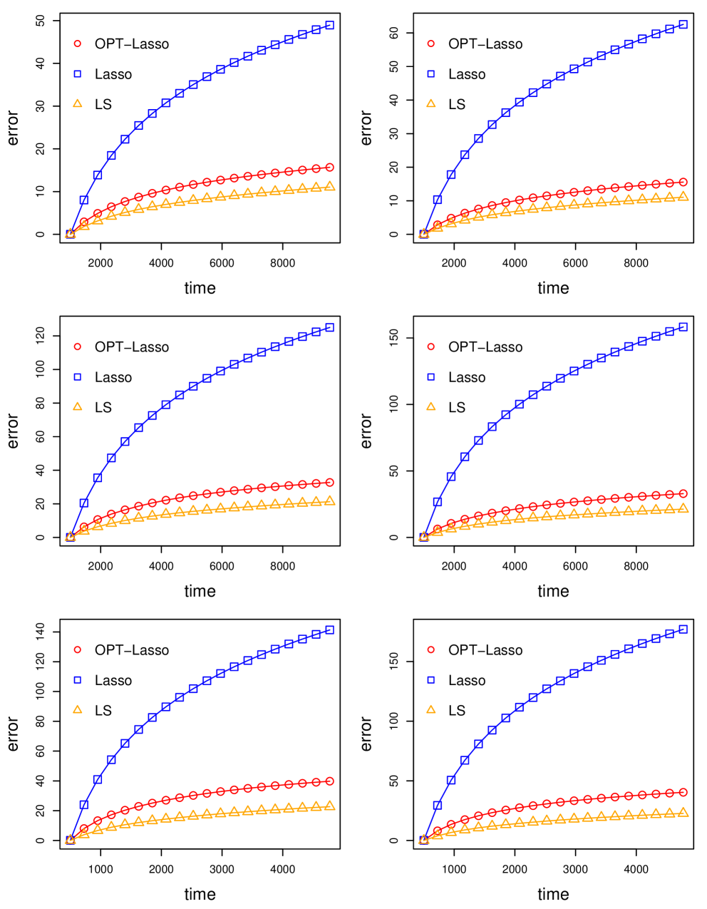
Figure 6: The $x$-axis represents time, and the $y$-axis shows the cumulative estimation error from time $T/10$ to time $t\in[T/10,T]$. The three rows correspond to scenarios (a), (b), and (d), respectively, while the first and second columns correspond to the parameter settings $(C_{0}=0.8,\ C_{0}^{\textup{hard}}=0.6)$ and $(C_{0}=1,\ C_{0}^{\textup{hard}}=0.4)$, respectively. Each plot displays the running cumulative estimation error of OPT-Lasso, Lasso, and an oracle estimator (denoted as “LS”), which has access to the true support.

Table 4: Under four scenarios, for different combinations of $C_{0}$ and $C_{0}^{\textup{hard}}$, we report the cumulative estimation error from time $T/10$ to $T$ for OPT-Lasso and Lasso. The combinations with the smallest cumulative errors are marked in bold.

(a)			OPT-Lasso			Lasso
$C_{0}\;\backslash\;C_{0}^{\textup{hard}}$	0.2	0.4	0.6	0.8	2.0	-
0.4	176.8 $\pm$ 7.7	135.3 $\pm$ 2.1	100.0 $\pm$ 1.1	69.7 $\pm$ 1.0	16.1 $\pm$ 0.8	64.2 $\pm$ 1.4
0.6	99.0 $\pm$ 1.1	56.7 $\pm$ 1.3	31.7 $\pm$ 0.6	20.1 $\pm$ 0.4	23.9 $\pm$ 1.4	45.7 $\pm$ 1.1
0.8	46.3 $\pm$ 1.5	22.7 $\pm$ 0.5	16.0 $\pm$ 0.4	15.9 $\pm$ 0.7	41.0 $\pm$ 2.3	52.5 $\pm$ 1.5
1.0	23.1 $\pm$ 0.8	15.9 $\pm$ 0.3	17.2 $\pm$ 0.4	21.9 $\pm$ 1.1	70.0 $\pm$ 3.9	64.6 $\pm$ 1.4
1.2	16.7 $\pm$ 0.4	16.9 $\pm$ 0.4	20.4 $\pm$ 1.0	26.1 $\pm$ 0.8	102.4 $\pm$ 6.1	88.5 $\pm$ 1.9

(b)			OPT-Lasso			Lasso
$C_{0}\;\backslash\;C_{0}^{\textup{hard}}$	0.2	0.4	0.6	0.8	2.0	-
0.4	761.6 $\pm$ 4.9	482.0 $\pm$ 26.4	356.3 $\pm$ 9.6	224.2 $\pm$ 4.9	33.6 $\pm$ 0.9	203.9 $\pm$ 2.6
0.6	322.9 $\pm$ 5.4	156.5 $\pm$ 2.6	74.7 $\pm$ 1.2	42.1 $\pm$ 1.0	53.2 $\pm$ 1.7	124.4 $\pm$ 1.4
0.8	115.7 $\pm$ 1.6	47.4 $\pm$ 1.0	33.3 $\pm$ 0.9	35.3 $\pm$ 0.8	94.4 $\pm$ 4.9	120.7 $\pm$ 2.2
1.0	46.3 $\pm$ 1.0	33.5 $\pm$ 0.7	39.6 $\pm$ 1.0	47.1 $\pm$ 1.2	171.2 $\pm$ 6.0	162.4 $\pm$ 2.1
1.2	34.2 $\pm$ 0.9	37.4 $\pm$ 0.9	50.6 $\pm$ 1.7	65.8 $\pm$ 1.8	272.9 $\pm$ 13.0	222.0 $\pm$ 4.0

(c)			OPT-Lasso			Lasso
$C_{0}\;\backslash\;C_{0}^{\textup{hard}}$	0.2	0.4	0.6	0.8	2.0	-
0.4	1108.6 $\pm$ 2.6	794.9 $\pm$ 2.3	515.1 $\pm$ 2.0	308.5 $\pm$ 1.7	23.8 $\pm$ 1.0	258.9 $\pm$ 1.8
0.6	468.6 $\pm$ 2.2	207.8 $\pm$ 2.1	79.6 $\pm$ 0.8	33.3 $\pm$ 0.5	36.3 $\pm$ 1.8	113.8 $\pm$ 1.4
0.8	144.3 $\pm$ 1.1	40.8 $\pm$ 0.5	21.1 $\pm$ 0.4	21.7 $\pm$ 0.4	68.3 $\pm$ 2.1	79.9 $\pm$ 1.1
1.0	38.6 $\pm$ 0.5	20.6 $\pm$ 0.4	24.2 $\pm$ 0.5	30.4 $\pm$ 0.6	121.3 $\pm$ 6.4	94.3 $\pm$ 1.9
1.2	20.4 $\pm$ 0.4	23.8 $\pm$ 0.5	31.9 $\pm$ 0.7	42.2 $\pm$ 0.9	196.1 $\pm$ 5.5	118.7 $\pm$ 1.4

(d)			OPT-Lasso			Lasso
$C_{0}\;\backslash\;C_{0}^{\textup{hard}}$	0.2	0.4	0.6	0.8	2.0	-
0.4	1122.1 $\pm$ 3.2	815.6 $\pm$ 2.8	534.3 $\pm$ 2.1	316.8 $\pm$ 1.6	41.6 $\pm$ 0.8	294.1 $\pm$ 1.5
0.6	487.8 $\pm$ 1.9	225.8 $\pm$ 1.4	97.3 $\pm$ 1.3	49.9 $\pm$ 0.6	73.7 $\pm$ 1.2	157.7 $\pm$ 0.9
0.8	162.1 $\pm$ 1.3	60.3 $\pm$ 1.0	40.5 $\pm$ 0.8	42.9 $\pm$ 0.6	136.5 $\pm$ 2.2	144.9 $\pm$ 1.0
1.0	57.4 $\pm$ 0.6	41.0 $\pm$ 0.6	47.6 $\pm$ 0.7	61.4 $\pm$ 1.4	239.0 $\pm$ 3.5	182.0 $\pm$ 1.2
1.2	40.2 $\pm$ 0.7	48.5 $\pm$ 1.0	66.3 $\pm$ 1.1	87.0 $\pm$ 1.4	403.0 $\pm$ 5.1	241.6 $\pm$ 1.4

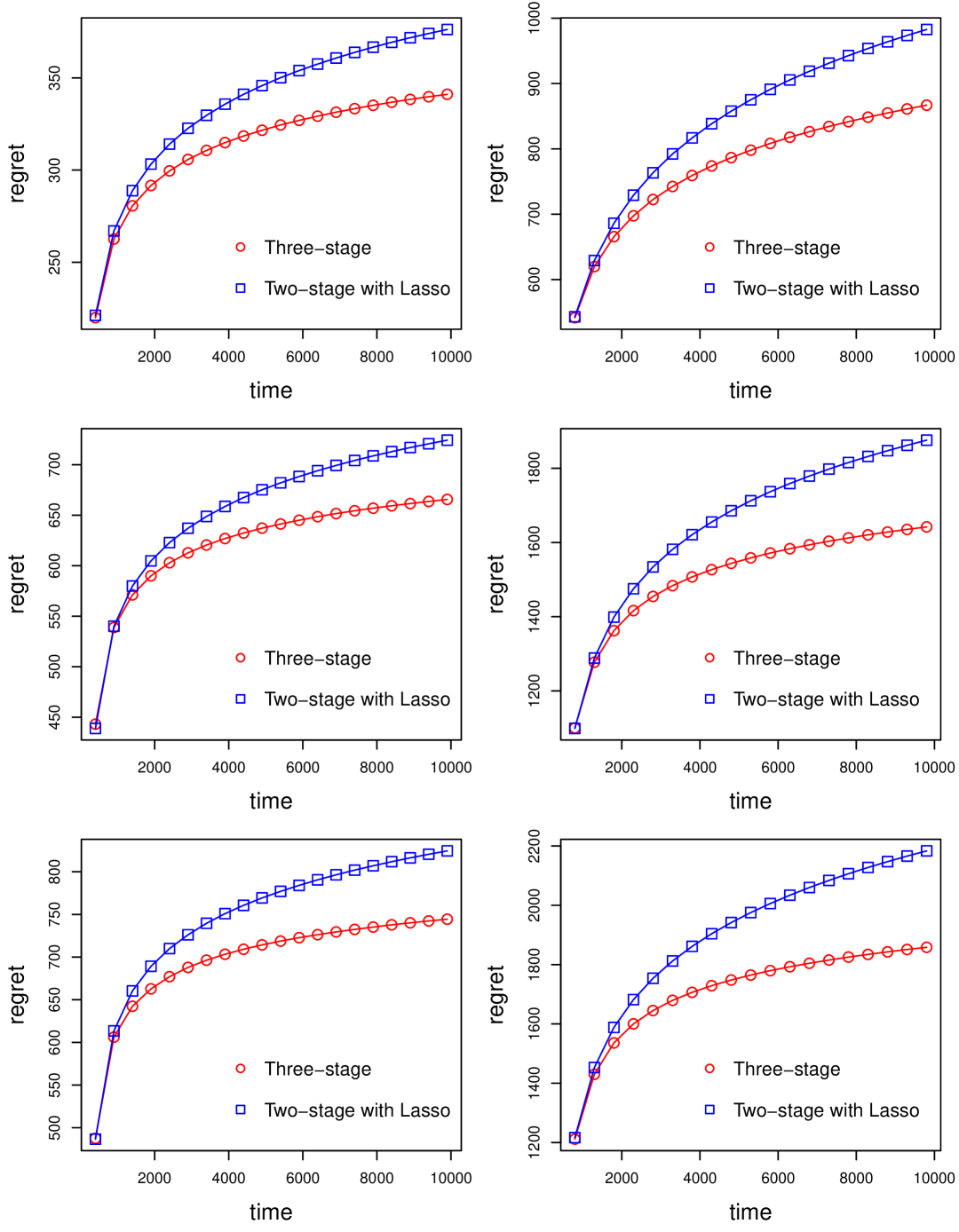
Figure 7: The $x$-axis represents time, and the $y$-axis denotes the cumulative regret up to time $t\in[\gamma_{2},T]$. The three rows in the left column correspond to scenarios (a), (c), and (g), with $C_{0}=2$ and $C_{0}^{\textup{hard}}=0.6$, while the three rows in the right column correspond to scenarios (b), (d), and (h), with $C_{0}=2$ and $C_{0}^{\textup{hard}}=1$.

Table 5: The tables show the cumulative regret for scenarios (a), (b), (c), (d), (g) and (h). The parameter combinations with the smallest cumulative regret are marked in bold.

$(a)$ $C_{0}\;\backslash\;C_{0}^{\textup{hard}}$ 0.2 0.6 1.0 1.5 2.0 1.0 826.2 $\pm$ 2.9 607.3 $\pm$ 2.3 441.0 $\pm$ 1.4 355.4 $\pm$ 1.1 351.0 $\pm$ 1.1 1.6 526.0 $\pm$ 2.1 361.4 $\pm$ 1.7 341.0 $\pm$ 1.5 405.6 $\pm$ 2.2 503.2 $\pm$ 3.1 2.0 416.8 $\pm$ 1.9 341.4 $\pm$ 1.6 388.6 $\pm$ 2.0 520.9 $\pm$ 3.1 721.5 $\pm$ 5.0 2.6 356.2 $\pm$ 1.7 398.0 $\pm$ 2.0 525.4 $\pm$ 3.3 813.5 $\pm$ 5.4 1258.5 $\pm$ 8.5 3.0 366.7 $\pm$ 1.8 466.1 $\pm$ 2.7 670.5 $\pm$ 4.4 1107.5 $\pm$ 7.9 1740.3 $\pm$ 10.7

$(b)$ $C_{0}\;\backslash\;C_{0}^{\textup{hard}}$ 0.2 0.6 1.0 1.5 2.0 1.0 2166.8 $\pm$ 4.4 1879.5 $\pm$ 4.0 1546.9 $\pm$ 2.8 1211.7 $\pm$ 2.4 1014.4 $\pm$ 2.2 1.6 1664.5 $\pm$ 4.0 1237.2 $\pm$ 3.7 967.2 $\pm$ 3.3 872.5 $\pm$ 3.1 920.5 $\pm$ 3.5 2.0 1401.0 $\pm$ 3.7 1000.3 $\pm$ 3.3 869.1 $\pm$ 2.8 916.1 $\pm$ 3.6 1082.7 $\pm$ 4.5 2.6 1112.5 $\pm$ 3.4 877.6 $\pm$ 3.1 918.3 $\pm$ 3.6 1131.9 $\pm$ 4.9 1510.1 $\pm$ 7.9 3.0 1009.3 $\pm$ 3.5 891.7 $\pm$ 3.4 1018.4 $\pm$ 4.6 1365.0 $\pm$ 6.6 1929.6 $\pm$ 10.5

$(c)$ $C_{0}\;\backslash\;C_{0}^{\textup{hard}}$ 0.2 0.6 1.0 1.5 2.0 1.0 1668.7 $\pm$ 3.7 1155.4 $\pm$ 3.1 793.2 $\pm$ 1.4 664.0 $\pm$ 1.2 688.4 $\pm$ 1.3 1.6 1007.7 $\pm$ 2.7 674.1 $\pm$ 2.1 673.4 $\pm$ 2.1 797.8 $\pm$ 2.7 1017.9 $\pm$ 4.0 2.0 781.8 $\pm$ 2.5 666.0 $\pm$ 2.2 776.2 $\pm$ 2.7 1028.8 $\pm$ 4.2 1418.2 $\pm$ 6.2 2.6 682.1 $\pm$ 2.4 774.3 $\pm$ 2.7 1042.1 $\pm$ 4.0 1576.0 $\pm$ 7.1 2360.6 $\pm$ 10.4 3.0 702.3 $\pm$ 2.4 905.3 $\pm$ 3.3 1309.9 $\pm$ 5.6 2096.3 $\pm$ 9.2 3161.9 $\pm$ 12.3

$(d)$ $C_{0}\;\backslash\;C_{0}^{\textup{hard}}$ 0.2 0.6 1.0 1.5 2.0 1.0 4263.2 $\pm$ 6.4 3614.1 $\pm$ 6.3 2832.8 $\pm$ 3.0 2108.4 $\pm$ 2.6 1779.4 $\pm$ 2.3 1.6 3177.1 $\pm$ 5.6 2242.0 $\pm$ 4.5 1741.6 $\pm$ 4.1 1674.8 $\pm$ 4.1 1852.6 $\pm$ 4.9 2.0 2623.9 $\pm$ 5.1 1810.8 $\pm$ 4.1 1644.5 $\pm$ 4.2 1827.6 $\pm$ 4.6 2218.2 $\pm$ 7.0 2.6 2070.1 $\pm$ 4.9 1652.3 $\pm$ 3.9 1813.7 $\pm$ 5.1 2309.7 $\pm$ 7.1 3084.4 $\pm$ 10.8 3.0 1861.3 $\pm$ 4.4 1706.8 $\pm$ 4.4 2039.1 $\pm$ 5.9 2790.1 $\pm$ 9.1 3869.8 $\pm$ 13.3

$(g)$ $C_{0}\;\backslash\;C_{0}^{\textup{hard}}$ 0.2 0.6 1.0 1.5 2.0 1.0 2129.6 $\pm$ 4.7 1404.3 $\pm$ 3.4 905.1 $\pm$ 2.8 745.2 $\pm$ 2.2 779.9 $\pm$ 2.4 1.6 1239.8 $\pm$ 3.3 759.1 $\pm$ 2.5 755.6 $\pm$ 2.5 904.0 $\pm$ 3.2 1154.0 $\pm$ 4.4 2.0 923.6 $\pm$ 2.7 744.8 $\pm$ 2.5 863.4 $\pm$ 2.7 1157.1 $\pm$ 4.7 1609.4 $\pm$ 6.7 2.6 765.5 $\pm$ 2.4 856.2 $\pm$ 2.9 1164.2 $\pm$ 4.5 1763.5 $\pm$ 7.4 2636.6 $\pm$ 10.6 3.0 778.8 $\pm$ 2.5 999.2 $\pm$ 3.8 1460.9 $\pm$ 6.3 2336.2 $\pm$ 10.1 3456.2 $\pm$ 13.8

$(h)$ $C_{0}\;\backslash\;C_{0}^{\textup{hard}}$ 0.2 0.6 1.0 1.5 2.0 1.0 4935.7 $\pm$ 7.1 4227.7 $\pm$ 6.8 3246.3 $\pm$ 5.9 2336.2 $\pm$ 4.9 1986.5 $\pm$ 4.8 1.6 3817.5 $\pm$ 6.3 2597.0 $\pm$ 5.6 1963.8 $\pm$ 4.3 1906.1 $\pm$ 4.6 2130.3 $\pm$ 5.8 2.0 3138.4 $\pm$ 5.8 2069.7 $\pm$ 4.9 1861.3 $\pm$ 4.7 2104.8 $\pm$ 5.8 2557.4 $\pm$ 7.8 2.6 2422.7 $\pm$ 5.3 1854.3 $\pm$ 4.8 2069.9 $\pm$ 5.4 2658.4 $\pm$ 8.4 3575.2 $\pm$ 12.4 3.0 2149.2 $\pm$ 4.9 1909.7 $\pm$ 4.8 2297.2 $\pm$ 7.0 3197.0 $\pm$ 10.9 4505.6 $\pm$ 16.2

References

- [1] {barticle}[author] \bauthor\bsnmAbbasi-Yadkori, \bfnmYasin\binitsY., \bauthor\bsnmPál, \bfnmDávid\binitsD. and \bauthor\bsnmSzepesvári, \bfnmCsaba\binitsC. (\byear2011). \btitleImproved algorithms for linear stochastic bandits. \bjournalAdvances in neural information processing systems \bvolume24 \bpages2312–2320. \endbibitem
- [2] {binproceedings}[author] \bauthor\bsnmAgrawal, \bfnmShipra\binitsS. and \bauthor\bsnmGoyal, \bfnmNavin\binitsN. (\byear2012). \btitleAnalysis of thompson sampling for the multi-armed bandit problem. In \bbooktitleConference on learning theory \bpages39–1. \bpublisherJMLR Workshop and Conference Proceedings. \endbibitem
- [3] {binproceedings}[author] \bauthor\bsnmAriu, \bfnmKaito\binitsK., \bauthor\bsnmAbe, \bfnmKenshi\binitsK. and \bauthor\bsnmProutière, \bfnmAlexandre\binitsA. (\byear2022). \btitleThresholded lasso bandit. In \bbooktitleInternational Conference on Machine Learning \bpages878–928. \bpublisherPMLR. \endbibitem
- [4] {binproceedings}[author] \bauthor\bsnmAudibert, \bfnmJean-Yves\binitsJ.-Y. and \bauthor\bsnmBubeck, \bfnmSébastien\binitsS. (\byear2009). \btitleMinimax Policies for Adversarial and Stochastic Bandits. In \bbooktitle22nd Conference on Learning Theory \bvolume217–226. \endbibitem
- [5] {barticle}[author] \bauthor\bsnmAuer, \bfnmPeter\binitsP., \bauthor\bsnmCesa-Bianchi, \bfnmNicolo\binitsN. and \bauthor\bsnmFischer, \bfnmPaul\binitsP. (\byear2002). \btitleFinite-time analysis of the multiarmed bandit problem. \bjournalMachine learning \bvolume47 \bpages235–256. \endbibitem
- [6] {barticle}[author] \bauthor\bsnmAuer, \bfnmPeter\binitsP., \bauthor\bsnmCesa-Bianchi, \bfnmNicolo\binitsN., \bauthor\bsnmFreund, \bfnmYoav\binitsY. and \bauthor\bsnmSchapire, \bfnmRobert E\binitsR. E. (\byear2002). \btitleThe nonstochastic multiarmed bandit problem. \bjournalSIAM journal on computing \bvolume32 \bpages48–77. \endbibitem
- [7] {barticle}[author] \bauthor\bsnmBastani, \bfnmHamsa\binitsH. and \bauthor\bsnmBayati, \bfnmMohsen\binitsM. (\byear2020). \btitleOnline decision making with high-dimensional covariates. \bjournalOperations Research \bvolume68 \bpages276–294. \endbibitem
- [8] {barticle}[author] \bauthor\bsnmBastani, \bfnmHamsa\binitsH., \bauthor\bsnmBayati, \bfnmMohsen\binitsM. and \bauthor\bsnmKhosravi, \bfnmKhashayar\binitsK. (\byear2021). \btitleMostly exploration-free algorithms for contextual bandits. \bjournalManagement Science \bvolume67 \bpages1329–1349. \endbibitem
- [9] {barticle}[author] \bauthor\bsnmBellec, \bfnmPierre C\binitsP. C. and \bauthor\bsnmZhang, \bfnmCun-Hui\binitsC.-H. (\byear2022). \btitleDe-biasing the lasso with degrees-of-freedom adjustment. \bjournalBernoulli \bvolume28 \bpages713–743. \endbibitem
- [10] {barticle}[author] \bauthor\bsnmBelloni, \bfnmAlexandre\binitsA. and \bauthor\bsnmChernozhukov, \bfnmVictor\binitsV. (\byear2013). \btitleLeast squares after model selection in high-dimensional sparse models. \bjournalBernoulli \bvolume19 \bpages521–547. \endbibitem
- [11] {barticle}[author] \bauthor\bsnmBubeck, \bfnmSébastien\binitsS. and \bauthor\bsnmCesa-Bianchi, \bfnmNicolò\binitsN. (\byear2012). \btitleRegret Analysis of Stochastic and Nonstochastic Multi-armed Bandit Problems. \bjournalFound. Trends Mach. Learn. \bvolume5 \bpages1–122. \bdoi10.1561/2200000024 \endbibitem
- [12] {bbook}[author] \bauthor\bsnmBühlmann, \bfnmPeter\binitsP. and \bauthor\bsnmVan De Geer, \bfnmSara\binitsS. (\byear2011). \btitleStatistics for high-dimensional data: methods, theory and applications. \bpublisherSpringer Science & Business Media. \endbibitem
- [13] {barticle}[author] \bauthor\bsnmChapelle, \bfnmOlivier\binitsO. and \bauthor\bsnmLi, \bfnmLihong\binitsL. (\byear2011). \btitleAn empirical evaluation of thompson sampling. \bjournalAdvances in neural information processing systems \bvolume24. \endbibitem
- [14] {binproceedings}[author] \bauthor\bsnmDing, \bfnmQin\binitsQ., \bauthor\bsnmHsieh, \bfnmCho-Jui\binitsC.-J. and \bauthor\bsnmSharpnack, \bfnmJames\binitsJ. (\byear2021). \btitleAn efficient algorithm for generalized linear bandit: Online stochastic gradient descent and thompson sampling. In \bbooktitleInternational Conference on Artificial Intelligence and Statistics \bpages1585–1593. \bpublisherPMLR. \endbibitem
- [15] {barticle}[author] \bauthor\bsnmGill, \bfnmRichard D\binitsR. D. and \bauthor\bsnmLevit, \bfnmBoris Y\binitsB. Y. (\byear1995). \btitleApplications of the van Trees inequality: a Bayesian Cramér-Rao bound. \bjournalBernoulli \bpages59–79. \endbibitem
- [16] {barticle}[author] \bauthor\bsnmGoldenshluger, \bfnmAlexander\binitsA. and \bauthor\bsnmZeevi, \bfnmAssaf\binitsA. (\byear2013). \btitleA linear response bandit problem. \bjournalStochastic Systems \bvolume3 \bpages230–261. \endbibitem
- [17] {barticle}[author] \bauthor\bsnmHamidi, \bfnmNima\binitsN. and \bauthor\bsnmBayati, \bfnmMohsen\binitsM. (\byear2020). \btitleA General Framework to Analyze Stochastic Linear Bandit. \bjournalCoRR \bvolumeabs/2002.05152. \endbibitem
- [18] {barticle}[author] \bauthor\bsnmHao, \bfnmBotao\binitsB., \bauthor\bsnmLattimore, \bfnmTor\binitsT. and \bauthor\bsnmWang, \bfnmMengdi\binitsM. (\byear2020). \btitleHigh-dimensional sparse linear bandits. \bjournalAdvances in Neural Information Processing Systems \bvolume33 \bpages10753–10763. \endbibitem
- [19] {barticle}[author] \bauthor\bsnmJin, \bfnmChi\binitsC., \bauthor\bsnmNetrapalli, \bfnmPraneeth\binitsP., \bauthor\bsnmGe, \bfnmRong\binitsR., \bauthor\bsnmKakade, \bfnmSham M\binitsS. M. and \bauthor\bsnmJordan, \bfnmMichael I\binitsM. I. (\byear2019). \btitleA short note on concentration inequalities for random vectors with subgaussian norm. \bjournalarXiv preprint arXiv:1902.03736. \endbibitem
- [20] {barticle}[author] \bauthor\bsnmJun, \bfnmKwang-Sung\binitsK.-S., \bauthor\bsnmBhargava, \bfnmAniruddha\binitsA., \bauthor\bsnmNowak, \bfnmRobert\binitsR. and \bauthor\bsnmWillett, \bfnmRebecca\binitsR. (\byear2017). \btitleScalable generalized linear bandits: Online computation and hashing. \bjournalAdvances in Neural Information Processing Systems \bvolume30. \endbibitem
- [21] {binproceedings}[author] \bauthor\bsnmKakade, \bfnmSham M\binitsS. M., \bauthor\bsnmShalev-Shwartz, \bfnmShai\binitsS. and \bauthor\bsnmTewari, \bfnmAmbuj\binitsA. (\byear2008). \btitleEfficient bandit algorithms for online multiclass prediction. In \bbooktitleProceedings of the 25th international conference on Machine learning \bpages440–447. \endbibitem
- [22] {barticle}[author] \bauthor\bsnmKim, \bfnmGi-Soo\binitsG.-S. and \bauthor\bsnmPaik, \bfnmMyunghee Cho\binitsM. C. (\byear2019). \btitleDoubly-robust lasso bandit. \bjournalAdvances in Neural Information Processing Systems \bvolume32. \endbibitem
- [23] {barticle}[author] \bauthor\bsnmLai, \bfnmTze Leung\binitsT. L., \bauthor\bsnmRobbins, \bfnmHerbert\binitsH. \betalet al. (\byear1985). \btitleAsymptotically efficient adaptive allocation rules. \bjournalAdvances in applied mathematics \bvolume6 \bpages4–22. \endbibitem
- [24] {bbook}[author] \bauthor\bsnmLattimore, \bfnmTor\binitsT. and \bauthor\bsnmSzepesvári, \bfnmCsaba\binitsC. (\byear2020). \btitleBandit algorithms. \bpublisherCambridge University Press. \endbibitem
- [25] {binproceedings}[author] \bauthor\bsnmLi, \bfnmLihong\binitsL., \bauthor\bsnmChu, \bfnmWei\binitsW., \bauthor\bsnmLangford, \bfnmJohn\binitsJ. and \bauthor\bsnmSchapire, \bfnmRobert E.\binitsR. E. (\byear2010). \btitleA contextual-bandit approach to personalized news article recommendation. In \bbooktitleProceedings of the 19th International Conference on World Wide Web \bpages661–670. \bpublisherACM. \endbibitem
- [26] {binproceedings}[author] \bauthor\bsnmLi, \bfnmLihong\binitsL., \bauthor\bsnmChu, \bfnmWei\binitsW., \bauthor\bsnmLangford, \bfnmJohn\binitsJ. and \bauthor\bsnmSchapire, \bfnmRobert E\binitsR. E. (\byear2010). \btitleA contextual-bandit approach to personalized news article recommendation. In \bbooktitleProceedings of the 19th international conference on World wide web \bpages661–670. \endbibitem
- [27] {binproceedings}[author] \bauthor\bsnmOh, \bfnmMin-hwan\binitsM.-h., \bauthor\bsnmIyengar, \bfnmGarud\binitsG. and \bauthor\bsnmZeevi, \bfnmAssaf\binitsA. (\byear2021). \btitleSparsity-agnostic lasso bandit. In \bbooktitleInternational Conference on Machine Learning \bpages8271–8280. \bpublisherPMLR. \endbibitem
- [28] {barticle}[author] \bauthor\bsnmPerchet, \bfnmVianney\binitsV. and \bauthor\bsnmRigollet, \bfnmPhilippe\binitsP. (\byear2013). \btitleThe multi-armed bandit problem with covariates. \bjournalThe Annals of Statistics \bvolume41 \bpages693–721. \endbibitem
- [29] {barticle}[author] \bauthor\bsnmRaskutti, \bfnmGarvesh\binitsG., \bauthor\bsnmWainwright, \bfnmMartin J\binitsM. J. and \bauthor\bsnmYu, \bfnmBin\binitsB. (\byear2011). \btitleMinimax rates of estimation for high-dimensional linear regression over -balls. \bjournalIEEE transactions on information theory \bvolume57 \bpages6976–6994. \endbibitem
- [30] {barticle}[author] \bauthor\bsnmRen, \bfnmZhimei\binitsZ. and \bauthor\bsnmZhou, \bfnmZhengyuan\binitsZ. (\byear2024). \btitleDynamic batch learning in high-dimensional sparse linear contextual bandits. \bjournalManagement Science \bvolume70 \bpages1315–1342. \endbibitem
- [31] {bmisc}[author] \bauthor\bsnmRigollet, \bfnmPhilippe\binitsP. and \bauthor\bsnmHütter, \bfnmJan-Christian\binitsJ.-C. (\byear2023). \btitleHigh-Dimensional Statistics. \endbibitem
- [32] {barticle}[author] \bauthor\bsnmRobbins, \bfnmHerbert\binitsH. (\byear1952). \btitleSome aspects of the sequential design of experiments. \bjournalBulletin of the American Mathematical Society \bvolume58 \bpages527–535. \endbibitem
- [33] {binproceedings}[author] \bauthor\bsnmRudelson, \bfnmMark\binitsM. and \bauthor\bsnmZhou, \bfnmShuheng\binitsS. (\byear2012). \btitleReconstruction from Anisotropic Random Measurements. In \bbooktitleProceedings of the 25th Annual Conference on Learning Theory. \bseriesProceedings of Machine Learning Research \bvolume23 \bpages10.1–10.24. \bpublisherPMLR, \baddressEdinburgh, Scotland. \endbibitem
- [34] {barticle}[author] \bauthor\bsnmRusso, \bfnmDaniel\binitsD. and \bauthor\bsnmVan Roy, \bfnmBenjamin\binitsB. (\byear2018). \btitleLearning to optimize via information-directed sampling. \bjournalOperations Research \bvolume66 \bpages230–252. \endbibitem
- [35] {barticle}[author] \bauthor\bsnmShalev-Shwartz, \bfnmShai\binitsS. \betalet al. (\byear2012). \btitleOnline learning and online convex optimization. \bjournalFoundations and Trends® in Machine Learning \bvolume4 \bpages107–194. \endbibitem
- [36] {barticle}[author] \bauthor\bsnmSong, \bfnmYanglei\binitsY. and \bauthor\bsnmZhou, \bfnmMeng\binitsM. (\byear2022). \btitleTruncated LinUCB for Stochastic Linear Bandits. \bjournalarXiv preprint arXiv:2202.11735. \endbibitem
- [37] {bincollection}[author] \bauthor\bsnmTewari, \bfnmAmbuj\binitsA. and \bauthor\bsnmMurphy, \bfnmSusan A\binitsS. A. (\byear2017). \btitleFrom ads to interventions: Contextual bandits in mobile health. In \bbooktitleMobile Health \bpages495–517. \bpublisherSpringer. \endbibitem
- [38] {barticle}[author] \bauthor\bsnmThompson, \bfnmWilliam R\binitsW. R. (\byear1933). \btitleOn the likelihood that one unknown probability exceeds another in view of the evidence of two samples. \bjournalBiometrika \bvolume25 \bpages285–294. \endbibitem
- [39] {barticle}[author] \bauthor\bsnmTibshirani, \bfnmRobert\binitsR. (\byear1996). \btitleRegression shrinkage and selection via the lasso. \bjournalJournal of the Royal Statistical Society: Series B (Methodological) \bvolume58 \bpages267–288. \endbibitem
- [40] {barticle}[author] \bauthor\bparticleVan de \bsnmGeer, \bfnmSara\binitsS., \bauthor\bsnmBühlmann, \bfnmPeter\binitsP. and \bauthor\bsnmZhou, \bfnmShuheng\binitsS. (\byear2011). \btitleThe adaptive and the thresholded Lasso for potentially misspecified models (and a lower bound for the Lasso). \endbibitem
- [41] {barticle}[author] \bauthor\bparticleVan de \bsnmGeer, \bfnmSara A\binitsS. A. (\byear2008). \btitleHigh-dimensional generalized linear models and the lasso. \bjournalThe Annals of Statistics \bvolume36 \bpages614–645. \endbibitem
- [42] {bbook}[author] \bauthor\bparticleVan de \bsnmGeer, \bfnmSara A\binitsS. A. (\byear2016). \btitleEstimation and testing under sparsity. \bpublisherSpringer. \endbibitem
- [43] {bbook}[author] \bauthor\bsnmVershynin, \bfnmRoman\binitsR. (\byear2018). \btitleHigh-dimensional probability: An introduction with applications in data science \bvolume47. \bpublisherCambridge university press. \endbibitem
- [44] {barticle}[author] \bauthor\bsnmWainwright, \bfnmMartin J\binitsM. J. (\byear2009). \btitleSharp thresholds for High-Dimensional and noisy sparsity recovery using -Constrained Quadratic Programming (Lasso). \bjournalIEEE transactions on information theory \bvolume55 \bpages2183–2202. \endbibitem
- [45] {bbook}[author] \bauthor\bsnmWainwright, \bfnmMartin J\binitsM. J. (\byear2019). \btitleHigh-dimensional statistics: A non-asymptotic viewpoint \bvolume48. \bpublisherCambridge University Press. \endbibitem
- [46] {binproceedings}[author] \bauthor\bsnmWang, \bfnmXue\binitsX., \bauthor\bsnmWei, \bfnmMingcheng\binitsM. and \bauthor\bsnmYao, \bfnmTao\binitsT. (\byear2018). \btitleMinimax concave penalized multi-armed bandit model with high-dimensional covariates. In \bbooktitleInternational Conference on Machine Learning \bpages5200–5208. \bpublisherPMLR. \endbibitem
- [47] {barticle}[author] \bauthor\bsnmYuan, \bfnmMing\binitsM. and \bauthor\bsnmLin, \bfnmYi\binitsY. (\byear2006). \btitleModel selection and estimation in regression with grouped variables. \bjournalJournal of the Royal Statistical Society: Series B (Statistical Methodology) \bvolume68 \bpages49–67. \endbibitem
- [48] {barticle}[author] \bauthor\bsnmZhang, \bfnmCun-Hui\binitsC.-H. and \bauthor\bsnmHuang, \bfnmJian\binitsJ. (\byear2008). \btitleThe sparsity and bias of the Lasso selection in high-dimensional linear regression. \bjournalThe Annals of Statistics \bvolume36 \bpages1567 – 1594. \bdoi10.1214/07-AOS520 \endbibitem
- [49] {barticle}[author] \bauthor\bsnmZhao, \bfnmPeng\binitsP. and \bauthor\bsnmYu, \bfnmBin\binitsB. (\byear2006). \btitleOn model selection consistency of Lasso. \bjournalThe Journal of Machine Learning Research \bvolume7 \bpages2541–2563. \endbibitem
- [50] {barticle}[author] \bauthor\bsnmZou, \bfnmHui\binitsH. (\byear2006). \btitleThe adaptive lasso and its oracle properties. \bjournalJournal of the American statistical association \bvolume101 \bpages1418–1429. \endbibitem
- [51] {barticle}[author] \bauthor\bsnmZou, \bfnmHui\binitsH. and \bauthor\bsnmHastie, \bfnmTrevor\binitsT. (\byear2005). \btitleRegularization and variable selection via the elastic net. \bjournalJournal of the Royal Statistical Society Series B: Statistical Methodology \bvolume67 \bpages301–320. \endbibitem