Spectral Mixture Kernels for Bayesian Optimization

Abstract

Bayesian Optimization (BO) is a widely used approach for solving expensive black-box optimization tasks. However, selecting an appropriate probabilistic surrogate model remains an important yet challenging problem. In this work, we introduce a novel Gaussian Process (GP)-based BO method that incorporates spectral mixture kernels, derived from spectral densities formed by scale-location mixtures of Cauchy and Gaussian distributions. This method achieves a significant improvement in both efficiency and optimization performance, matching the computational speed of simpler kernels while delivering results that outperform more complex models and automatic BO methods. We provide bounds on the information gain and cumulative regret associated with obtaining the optimum. Extensive numerical experiments demonstrate that our method consistently outperforms existing baselines across a diverse range of synthetic and real-world problems, including both low- and high-dimensional settings.

1 Introduction

Gradient-free optimization of expensive black-box functions is a ubiquitous task in many fields. Bayesian Optimization (BO) has emerged as a mainstream approach to tackle those difficulties Wang_2017 . Featuring expressive surrogate models and high data efficiency, BO has been applied across various fields to a wide class of problems, including but not limited to materials design and discovery Frazier_2016 , experimental design Lorenz_2019 , reinforcement learning Turchetta_2020 , hyperparameter tuning Wu_2020 , and neural architecture search Kandasamy_2018 . A typical BO algorithm has two key components that must be determined: (i) the acquisition function, i.e., the utility function guiding the search towards the most promising candidate solution; and (ii) the surrogate model, i.e., a probabilistic model used to approximate the expensive-to-evaluate objective function. Whereas the former has been studied extensively, e.g., expected improvement (EI) Mockus_1975 , knowledge gradient (KG) Frazier_2008 , Thompson sampling Agrawal_2012 , max-value entropy search Wang_2017 , etc, the choice of surrogate model has received relatively less attention.

In BO approaches, a surrogate model, often a Gaussian Process (GP) Rasmussen_2006 , provides a probabilistic belief over the unknown objective function. Covariance function, or kernel, is the crucial ingredient of GP, as it encodes assumptions about the objective function, e.g., smoothness, periodicity, etc. Therefore, the choice of kernel significantly influences BO performance by shaping the structure of the underlying GP surrogate. Most off-the-shelf BO solvers use general-purpose kernels, including squared exponential (SE), rational quadratic (RQ), periodic (PE), and Matérn kernels, etc. While these kernels are simple and widely used, they often lack expressiveness and may fail to capture the inherent complexity of real-world phenomena Wilson_2013 .

In this paper, we aim to derive flexible GP surrogates for BO by expressing covariance functions in terms of their Fourier transforms, specifically spectral mixture kernels. Our motivation stems from Bochner’s theorem Stein_1999 , which shows that every stationary kernel used in GP models is associated with a symmetric spectral measure. Building on this characterization, we propose BO with spectral mixture kernels, which offer a simple form while accommodating varying levels of complexity. Additionally, Fourier transformations are dense in stationary covariances, meaning any stationary kernel can be approximated to arbitrary precision, provided the spectral densities cover a sufficiently wide range Konstantinos_2000 ; Wilson_2013 . Thus, spectral mixture kernels can serve as a direct replacement for conventional kernels. In this regard, the traditional discrete search for conventional kernels in the spatial domain can now be replaced by continuous hyperparameter tuning in the Fourier domain. This approach enables us to achieve both the efficiency and simplicity of basic kernels, along with the expressiveness and flexibility of more complex composite kernels.

Specifically, we make the following contributions:

• Parameterize a new class of stationary kernels via Cauchy and Gaussian distributions in the Fourier domain, which provides distinct advantages over conventional kernels.

• Propose the first BO framework employing spectral mixture kernels, demonstrating the flexibility in optimizing black-box functions with complex spectral characteristics.

• Derive upper bounds for the information gain and cumulative regret in optimizing with spectral mixture kernels, and demonstrate their ability to approximate conventional stationary kernels and their compositions.

• Numerical results show improvements across all synthetic and real-world examples tested, including both low- and high-dimensional scenarios, with an average improvement of 11% compared to state-of-the-art baselines.

2 Related Work

BO with Kernel Designs

Conventional kernels, such as the SE or Matérn kernels, assume a fixed structure that may not capture the complexities of high-dimensional objective functions. To address this, several approaches have been proposed to design flexible kernels through automatic construction and adaptation. Kandasamy et al. Kandasamy_2015 introduced an additive structure for the objective function, decomposing it into a sum of lower-dimensional functions. This approach allows for efficient optimization in high-dimensional spaces by reducing the effective dimensionality of the problem. Building upon this, Gardner et al. Gardner_2017 proposed a method to automatically discover and exploit additive structures using a Metropolis-Hastings sampling algorithm. Their approach demonstrated improved performance by identifying hidden additive components in the objective function.

Malkomes et al. Malkomes_2018 introduced a dynamic approach to kernel construction during the BO process. They used a predefined grammar to iteratively combine basic kernels, enabling the exploration of a wide range of kernel compositions. While this approach offers greater flexibility, it also presents challenges in computational efficiency and risks overfitting due to the complexity of the kernel structures Wilson_2013 . To address the limitations of static kernel choices, adaptive kernel selection strategies have been explored Roman_2019_ADA . These strategies maintain a set of candidate kernels and dynamically select the most suitable one at each iteration based on six adaptive criteria. This adaptability allows the surrogate model to better respond to newly acquired data, which is particularly beneficial in the early stages of optimization when data is limited.

Despite the advancements in kernel design for BO, several challenges remain. The vast number of possible kernel compositions can make the search computationally expensive, and overly complex kernel structures may lead to overfitting and difficulties with hyperparameter inference.

Spectral Kernels

Recent developments in spectral kernels have notably enhanced the capabilities of GP modeling. A key advancement is the concept of sparse spectrum kernels Miguel_2010 , which are derived by sparsifying the spectral density of a full GP, resulting in a more efficient, sparse alternative. However, this class of kernels is prone to overfitting and implicitly assumes that the covariance between two points does not decay as their distance increases, an assumption that may not hold in many real-world, non-periodic applications Samo_2015 .

Wilson and Adams Wilson_2013 defined a space of stationary kernels using a family of Gaussian mixture distributions in the Fourier domain to represent the spectral density in GP regression. This formulation was later extended to handle multidimensional inputs by incorporating a Kronecker structure for scalability Wilson_2014 . However, the covariance functions induced by Gaussian mixture spectral densities are infinitely differentiable, which may be unrealistic for modeling certain physical processes Stein_1999 . While being introduced for regression tasks, the role of spectral mixture kernels in BO remains underexplored. In this paper, we propose and investigate the combination of Cauchy and Gaussian kernels into a spectral mixture, demonstrating state-of-the-art performance in optimization tasks.

The Sinc kernel Tobar_2019_SINC is another notable advancement, parameterizing the GP’s power spectral density as a rectangular function. This kernel has shown exceptional performance in signal processing, particularly in tasks like band-limited frequency recovery and anti-aliasing. The Spectral Delta kernel Vargas_2021_SDK approximates stationary kernels through a finite sum of cosine basis functions, offering computational efficiency by avoiding Fourier integrals. However, its expressiveness is constrained by the discrete frequency sampling and fixed amplitude scaling.

To address multi-channel dependencies, researchers have generalized spectral kernels to multi-output GP regressions. The Multi-Output Spectral Mixture kernel Parra_2017_SMK_multiGP explicitly models cross-covariances by representing them as complex-valued spectral mixtures, capturing inter-channel correlations within a parametric framework. Building on this, Altamirano and Tobar Altamirano_2022_multiGP proposed a nonstationary harmonizable kernel family, enabling time-varying cross-spectral density estimation for nonstationary processes. The Minecraft kernel Simpson_2021_Minecraft further innovates by structuring cross-covariances via block-diagonal spectral representations with rectangular step functions, enhancing interpretability for high-dimensional outputs.

3 Preliminaries

Bochner’s Theorem

Bochner’s Theorem provides a foundational result in characterizing positive definite kernels in terms of their spectral representations.

Theorem 3.1 (Bochner’s Theorem Bochner_1960 ).

A complex-valued function $k$ on $\mathbb{R}^{P}$ is the kernel of a weakly stationary, mean square continuous complex-valued random process on $\mathbb{R}^{P}$ if and only if it can be represented as

$$k(\tau)=\int_{\mathbb{R}^{P}}\exp(2\pi is^{\top}\tau)d\psi(s),$$

where $\psi$ is a positive finite Borel measure on $\mathbb{R}^{P}$.

Specifically, Bochner’s theorem states that the Fourier transform of any stationary covariance function on $\mathbb{R}^{P}$ is proportional to a probability measure, and conversely, the inverse Fourier transform of a probability measure yields a stationary covariance function Bochner_1960 ; Stein_1999 . The measure $\psi$ is called the spectral measure of $k$. If $\psi$ has a density $S$, then $S$ is referred to as the spectral density or power spectrum of $k$. The covariance function $k$ and the spectral density $S$ forms a Fourier pair Chatfield_2006 :

$$k(\tau)=\int S(s)\exp(2\pi is^{\top}\tau)\,ds,\qquad S(s)=\int k(\tau)\exp(-2\pi is^{\top}\tau)\,d\tau.$$ (1)

Mercer’s Theorem

Mercer’s Theorem is a central result in functional analysis that plays a crucial role in kernel methods, particularly in positive definite kernels. It provides a spectral decomposition of a positive definite kernel, allowing the kernel to be expressed in terms of its eigenvalues and eigenfunctions.

Theorem 3.2 (Mercer’s Theorem Knig_1986 ).

Let $(\mathcal{X},\psi)$ be a finite measure space and $k\in L_{\infty}(\mathcal{X}^{2},\psi^{2})$ be a kernel such that $T_{k}:L_{2}(\mathcal{X},\psi)\rightarrow L_{2}(\mathcal{X},\psi)$ is positive definite. Let $\phi_{i}\in L_{2}(\mathcal{X},\psi)$ be the normalized eigenfunctions of $T_{k}$ associated with the eigenvalues $\lambda_{i}>0$. Then:

1. The eigenvalues $\{\lambda_{i}\}_{i=1}^{\infty}$ are absolutely summable;

2. The kernel can be represented as $k(x,x^{\prime})=\sum_{i=1}^{\infty}\lambda_{i}\phi_{i}(x)\phi_{i}^{*}(x^{\prime}),$ which holds $\mu^{2}$ almost everywhere, with the series converging absolutely and uniformly $\mu^{2}$ almost everywhere.

Mercer’s Theorem allows us to express the kernel in terms of its eigenvalues and eigenfunctions, which reveals important information about the kernel’s smoothness. Specifically, processes with greater power at high frequencies show a slower eigenvalue decay, indicating lower smoothness.

4 Spectral Mixture Kernels

4.1 Gaussian Spectral Density

A natural choice for constructing a space of stationary kernels is to use a mixture of Gaussian distributions Wilson_2013 to represent the spectral density $S(s)$:

$$\phi_{\rm g}(s)=\sum_{q=1}^{Q_{g}}w_{q}\mathcal{N}(s;\mathbf{\mu}_{q},\mathbf{\Sigma}_{q}),\quad S(s)=\frac{\phi(s)+\phi(-s)}{2},$$ (2)

where the construction of $S$ ensures symmetry, and the wights $w_{q}$ determine the contribution of each of the $Q_{g}$ components. By taking the inverse Fourier transform in Eq. (1), the resulting spectral mixture kernel induced by Gaussian distributions (Gaussian spectral mixture kernel, GSM) is given by:

$$k_{\rm g}(\tau)=\sum_{q=1}^{Q_{g}}w_{q}\exp\left(-2\pi^{2}\tau^{\top}\mathbf{\Sigma}_{q}\tau\right)\cos\left(2\pi\tau^{\top}\mathbf{\mu}_{q}\right).$$ (3)

Inspecting Eq. (3), we observe that the covariance function induced by a Gaussian mixture spectral density is infinitely differentiable. However, this choice may generate overly smooth sample paths Garnett_2023 .

4.2 Cauchy Spectral Density

To address the issue of overly smooth sample paths in GSM, we introduce a different family of distributions, i.e., Cauchy distributions, to construct a class of continuous but finitely differentiable covariance functions.

Theorem 4.1.

If $\phi_{c}(s)$ is a mixture of $Q_{c}$ Cauchy distributions on $\mathbb{R}^{P}$, where the $q^{\text{th}}$ component has a position parameter vector $\mathbf{x_{0}}_{q}=({x_{0}}_{q}^{(1)},\ldots,{x_{0}}_{q}^{(P)})$ and scale parameter $\mathbf{\gamma_{q}}=\text{diag}(\gamma_{q}^{(1)},\ldots,\gamma_{q}^{(P)})$, and $\tau_{p}$ is the $p^{\text{th}}$ component of the $P$-dimensional vector $\mathbf{\tau}=\mathbf{x}-\mathbf{x^{\prime}}$. The Fourier dual of spectral density $\phi_{c}(s)$ is

$$k_{\rm c}(\mathbf{\tau})=\sum_{q=1}^{Q_{c}}w_{q}\exp\left(-2\pi|\mathbf{\tau}^{\top}\mathbf{\gamma_{q}}|\right)\cos\left(2\pi\mathbf{\tau}^{\top}\mathbf{{x_{0}}_{q}}\right).$$

The spectral mixture kernel induced by Cauchy distributions is referred to as the Cauchy spectral mixture kernel (CSM). We offer a brief outline of the key ideas here, and a detailed proof is provided in Appendix B.1.

We begin by considering a simplified case where the probability density function of a univariate Cauchy distribution is given by

$$\mathcal{C}(s;x_{0},\gamma)=\frac{1}{\pi}\frac{\gamma}{(s-x_{0})^{2}+\gamma^{2}},$$ (4)

and the spectral density $S$ follows Eq. (2), while replacing the Gaussian distribution with Cauchy distribution. Noting that $S$ is symmetric Rasmussen_2006 , substituting $S$ into Eq. (1) yields

$$k_{c}(\tau) =\frac{1}{\pi}\int\frac{\gamma}{(s-x_{0})^{2}+\gamma^{2}}\exp\left(2\pi is\tau\right)ds.$$

Notice that $\int_{-\infty}^{\infty}\frac{\gamma}{(s-x_{0})^{2}+\gamma^{2}}\,ds=\pi$, we have

$$\mathcal{F}\left[\frac{\gamma}{(s-x_{0})^{2}+\gamma^{2}}\right]=\exp(-2\pi|\gamma\tau|)\exp\left(2\pi ix_{0}\tau\right),$$

where $\mathcal{F}$ denotes the Fourier Transform. This gives us the following kernel

$$k_{\rm c}(\tau)=\exp\left(-2\pi|\gamma\tau|\right)\cos(2\pi\tau x_{0}).$$

Now, if $\phi(s)$ is a mixture of $Q_{c}$ Cauchy distributions as described in Theorem 4.1, with its spectral density given by $\phi_{\rm c}=\sum_{q=1}^{Q_{c}}w_{q}\mathcal{C}(s;\mathbf{x}_{0q},\mathbf{\gamma}_{q})$, we obtain

$$k_{\rm c}(\tau) =\sum_{q=1}^{Q_{c}}w_{q}\prod_{p=1}^{P}\exp\left(-2\pi|\tau_{p}\gamma_{q}^{(p)}|\right)\cos(2\pi\tau_{p}{x_{0}}_{q}^{(p)})=\sum_{q=1}^{Q_{c}}w_{q}\exp\left(-2\pi|\mathbf{\tau}^{\top}\mathbf{\gamma_{q}}|\right)\cos\left(2\pi\mathbf{\tau}^{\top}\mathbf{x_{0q}}\right).$$ (5)

4.3 Cauchy and Gaussian Spectral Mixture Kernel

To leverage the complementary properties of both distributions, we define a spectral density $S(s)$ as a mixture of Gaussian and Cauchy components:

$$\phi_{\rm cg}(s)=\sum_{q=1}^{Q_{g}}w_{q}^{g}\mathcal{N}(s;\mathbf{\mu}_{q},\mathbf{\Sigma}_{q})+\sum_{q=1}^{Q_{c}}w_{q}^{c}\mathcal{C}(s;\mathbf{x}_{0q},\mathbf{\gamma}_{q}).$$ (6)

The resulting Cauchy-Gaussian Spectral Mixture (CSM+GSM) then follows:

$$k_{\rm cg}(\mathbf{\tau})=\sum_{q=1}^{Q_{g}}w_{q}^{g}\exp\left(-2\pi^{2}\mathbf{\tau}^{\top}\mathbf{\Sigma}_{q}\mathbf{\tau}\right)\cos\left(2\pi\mathbf{\tau}^{\top}\mathbf{\mu}_{q}\right)+\sum_{q=1}^{Q_{c}}w_{q}^{c}\exp\left(-2\pi\mathbf{\tau}^{\top}\mathbf{\gamma}_{q}|\right)\cos\left(2\pi\mathbf{\tau}^{\top}\mathbf{x}_{0q}\right).$$ (7)

The CSM+GSM kernel offers several key advantages over using either component alone. First, it maintains spectral interpretability, where each component’s location parameters ($\mathbf{\mu}_{q}$ and $\mathbf{x}_{0q}$) correspond to distinct frequency modes and their weights represent relative energy contributions. Second, it achieves adaptive smoothness through multi-scale modeling capability. The Gaussian components capture smooth global trends via their bandwidth parameters $\mathbf{\Sigma}_{q}$ while the Cauchy components model local variations through their heavy-tailed distributions controlled by $\mathbf{\gamma}_{q}$. The pseudo-code for BO with spectral mixture kernels is presented in Appendix A.

5 Theoretical Analysis

5.1 Decay Rate

The eigenvalue decay of a kernel’s Mercer decomposition provides critical insights into its smoothness properties. Applying Mercer’s Theorem (Theorem 3.2) to both GSM and CSM reveals fundamental differences in their spectral characteristics.

For GSM in Eq. (3), the Mercer decomposition yields eigenvalues $\lambda_{i}^{g}$ with exponential decay:

$$\lambda_{i}^{g}\sim\exp\left(-\pi i/\bar{\sigma}\right),\quad\bar{\sigma}=\frac{1}{Q_{g}}\sum_{q=1}^{Q_{g}}\|\mathbf{\Sigma}_{q}^{1/2}\|,$$

where $\bar{\sigma}$ represents the average bandwidth of the Gaussian components. This rapid decay confirms that GSM generates infinitely differentiable sample paths, as:

$$\sum_{i=1}^{\infty}i^{2m}|\lambda_{i}^{g}|^{2}<\infty\quad\forall m\in\mathbb{N}.$$

Exponential decay corresponds to rapid, high-frequency attenuation, producing smooth functions. The decay rate $\propto\|\mathbf{\Sigma}_{q}\|^{-1}$ confirms that narrower Gaussians (smaller $\|\mathbf{\Sigma}_{q}\|$) yield faster decay.

CSM in Eq. (5) exhibits markedly different behavior. Its eigenvalues decay algebraically:

$$\lambda_{i}^{c}\sim i^{-(1+2\bar{\gamma})},\quad\bar{\gamma}=\frac{1}{Q_{c}}\sum_{q=1}^{Q_{c}}\|\mathbf{\gamma}_{q}\|,$$

with $\bar{\gamma}$ being the average scale parameter. This slower decay implies finite differentiability:

$$\sum_{i=1}^{\infty}i^{2m}|\lambda_{i}^{c}|^{2}<\infty\iff m<\bar{\gamma}.$$

Polynomial decay maintains significantly high-frequency components, enabling non-smooth function modeling. The exponent $-(1+2\bar{\gamma})$ shows that larger scale parameters $\gamma_{q}$ accelerate decay (increased smoothness). These decay rates are key to deriving the information gain and regret bound in the subsequent section.

5.2 Information Gain and Regret Bound

We first provide upper bounds on the maximum information gains of the spectral mixture kernels, which measure how fast the objective function $f$ can be learned in an information-theoretic sense. We refer readers to Appendix B.2 for the detailed proofs of the results in this section.

The maximum information gain $\gamma(T)$ achieved by sampling $T$ points in a GP defined over a set $\mathcal{X}\subset\mathbb{R}^{d}$ with a kernel $k$ is defined as:

$$\gamma(T):=\max_{A\subset\mathcal{X}:|A|=T}I(y_{A};f_{A}),$$

where $I(y_{A};f_{A})=\frac{1}{2}\log|I+\sigma^{-2}K_{A}|$. $K_{A}=[k(x,x^{\prime})]_{x,x^{\prime}\in A}$ is the covariance matrix of $f_{A}=[f(x)]_{x\in A}$ associated with the samples $A$, and $\sigma^{2}$ is the noise variance.

Theorem 5.1.

The upper bounds on the maximum information gain of CSM and GSM kernels are:

1. Cauchy spectral mixture (CSM): $\gamma_{c}(T)=\mathcal{O}\left(T^{\frac{d^{2}+d}{d^{2}+d+1}}(\log T)\right)$;

2. Gaussian spectral mixture (GSM): $\gamma_{g}(T)=\mathcal{O}\left((\log T)^{d+1}\right)$.

where $d$ denotes the input dimension.

Using maximum information gain, we apply Theorem 1 from Srinivas et al. Srinivas_2012 to derive the cumulative regret bound when pairing with a UCB acquisition function.

Proposition 5.2.

Let $\delta\in(0,1),\beta_{t}=2\log\left(|\mathcal{X}|t^{2}\pi^{2}/6\delta\right)$, where $\beta_{t}$ is the hyperparameter for the UCB acquisition function. Suppose the objective function $f:\mathcal{X}\rightarrow\mathbb{R}$ is sampled from $\mathcal{GP}(\boldsymbol{0},k(x,x^{\prime}))$. With high probability, BO using the UCB acquisition function obtains a cumulative regret bound of

1. Cauchy spectral mixture (CSM): $\mathcal{O}\left(T^{\frac{2d^{2}+2d+1}{2(d^{2}+d+1)}}\sqrt{\log T\cdot\log|\mathcal{X}|}\right),$

2. Gaussian spectral mixture (GSM): $\mathcal{O}\left(\sqrt{T}\cdot(\log T)^{\frac{d+1}{2}}\cdot\sqrt{\log|\mathcal{X}|}\right)$.

The information gain for the CSM kernel grows at a sub-polynomial rate in $T$. The exponent $\frac{d^{2}+d}{d^{2}+d+1}$ is slightly less than 1, implying that the information gain increases rapidly, but at a diminishing rate as $T$ grows. For the GSM kernel, the information gain grows logarithmically in $T$, with the growth rate amplified by the dimensionality $d$, indicating that higher dimensionality increases the rate of information gain. Due to its logarithmic growth in $T$, the GSM kernel more effectively controls cumulative regret, providing more stable long-term performance.

While our theoretical analysis establishes regret bounds for pure CSM and GSM, the CSM+GSM kernel suggests intriguing potential behavior. Intuitively, its mixed components imply dual-phase characteristics: in the initial optimization stages, the Cauchy components may promote high-frequency exploration, leading to polynomial information gain, while the asymptotic behavior is likely to transition to logarithmic scaling as the Gaussian components, which capture low-frequency patterns, become dominant. This phased behavior could provide a practical balance, achieving faster initial convergence compared to pure GSM while offering better long-term stability than pure CSM.

Example 5.3.

Figure 1 visualizes one iteration of BO using different kernels based on 6 random samples from a 1D test function $f(x)=\sin(x)+\sin(\frac{10}{3}x)$.

The results reveal significant divergence in the behavior of GP surrogates employing different kernels. CSM excels in capturing high-frequency components (rapid oscillations and narrow confidence bands around sharp peaks), aligning with its heavy-tailed spectral density that preserves high-frequency content; while GSM better models low-frequency trends (smooth fitting and wider confidence intervals) due to its exponentially decaying spectral density that attenuates high frequencies. The CSM+GSM achieves superior performance by maintaining CSM’s precise high-frequency tracking and GSM’s stable low-frequency extrapolation, as visually confirmed by its balanced error distribution and theoretically explained by its dual-peaked spectral energy distribution.

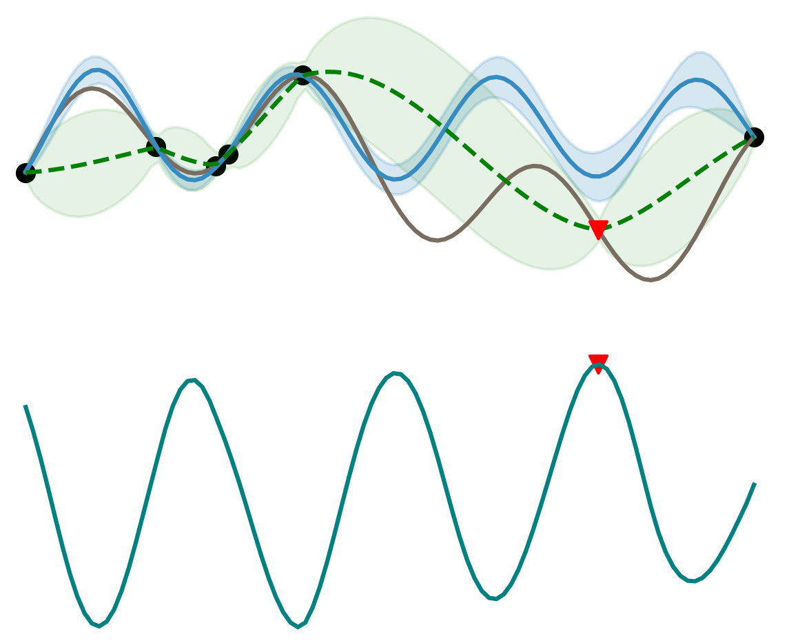
(a) CSM

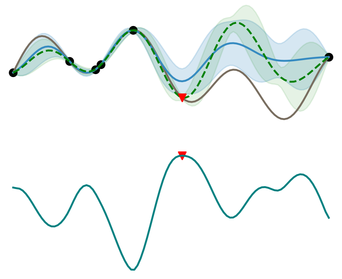
(b) GSM

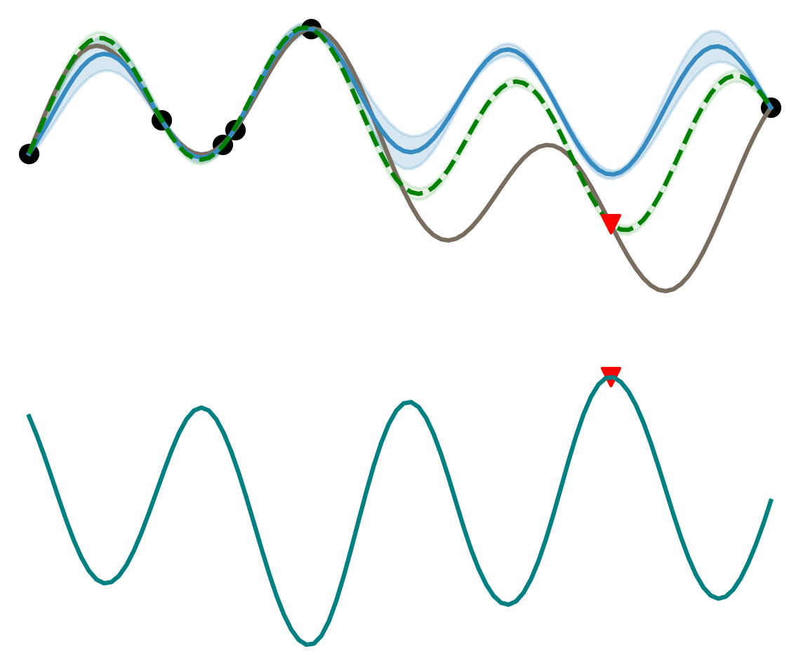
(c) CSM+GSM

Figure 1: Comparison of predictive distributions for the objective $f(x)$ using different kernels, before and after conditioning on the sampled point. The upper subplots show the GP surrogate before and after adding a new sample point, while the lower subplots display the corresponding acquisition function values using UCB and indicate the next point to sample.

6 Numerical Experiments

6.1 Approximate Conventional Kernels

Theorem 3.1 allows us to approximate an arbitrary stationary covariance function by approximating (e.g., modeling or sampling from) its spectral density Garnett_2023 . Since mixtures of Cauchy and Gaussian distributions can be used to construct a wide range of spectral densities Konstantinos_2000 , these mixtures enable us to approximate any stationary covariance function. We considered the approximation of conventional kernels of various complexities. The parameters for source kernels that generate the data are shown in Table 2 (Appendix C).

We evaluate the approximation ability of six distinct kernels, including the standard RQ, MA12, and MA52, alongside our proposed CSM, GSM, and CSM+GSM, through both quantitative and functional analyses. Table 1 reveals that our proposed kernels achieve superior marginal log likelihood (MLL) scores compared to conventional kernels. Figure 2 further demonstrates that our proposed kernels provide the closest approximation to the true kernel’s correlation structure.

Table 1: MLL of training on the sampled data. A higher MLL indicates a better approximation of the true kernel. Each experiment was repeated 10 times using different random seeds. The table shows the mean MLL values with standard deviations in parentheses.

	CSM+GSM	CSM	GSM	RQ	MA52	MA12	True
SE	$\mathbf{2.751}$ (0.067)	$2.719$ (0.075)	$2.702$ (0.059)	$2.498$ (0.058)	$2.437$ (0.058)	$2.256$ (0.061)	$2.752$ (0.044)
SE+MA32	$1.021$ (0.055)	$1.012$ (0.061)	1.042 (0.059)	$0.872$ (0.066)	$1.040$ (0.058)	$0.891$ (0.053)	$1.134$ (0.051)
SE*SE	$\mathbf{2.499}$ (0.059)	$2.271$ (0.054)	$2.398$ (0.056)	$2.292$ (0.065)	$1.933$ (0.058)	$1.728$ (0.063)	$2.517$ (0.045)
PE+SE+MA32	$\mathbf{0.885}$ (0.057)	$0.821$ (0.050)	$0.776$ (0.053)	$0.527$ (0.061)	$0.530$ (0.051)	$0.459$ (0.053)	$0.920$ (0.044)
SE*(PE+MA32)	$\mathbf{0.569}$ (0.049)	$0.521$ (0.053)	$0.557$ (0.044)	$0.418$ (0.052)	$0.534$ (0.042)	$0.377$ (0.043)	$0.575$ (0.041)
PE*(SE+MA32)	$\mathbf{0.983}$ (0.049)	$0.965$ (0.052)	$0.894$ (0.048)	$0.634$ (0.057)	$0.681$ (0.053)	$0.685$ (0.056)	$1.053$ (0.044)

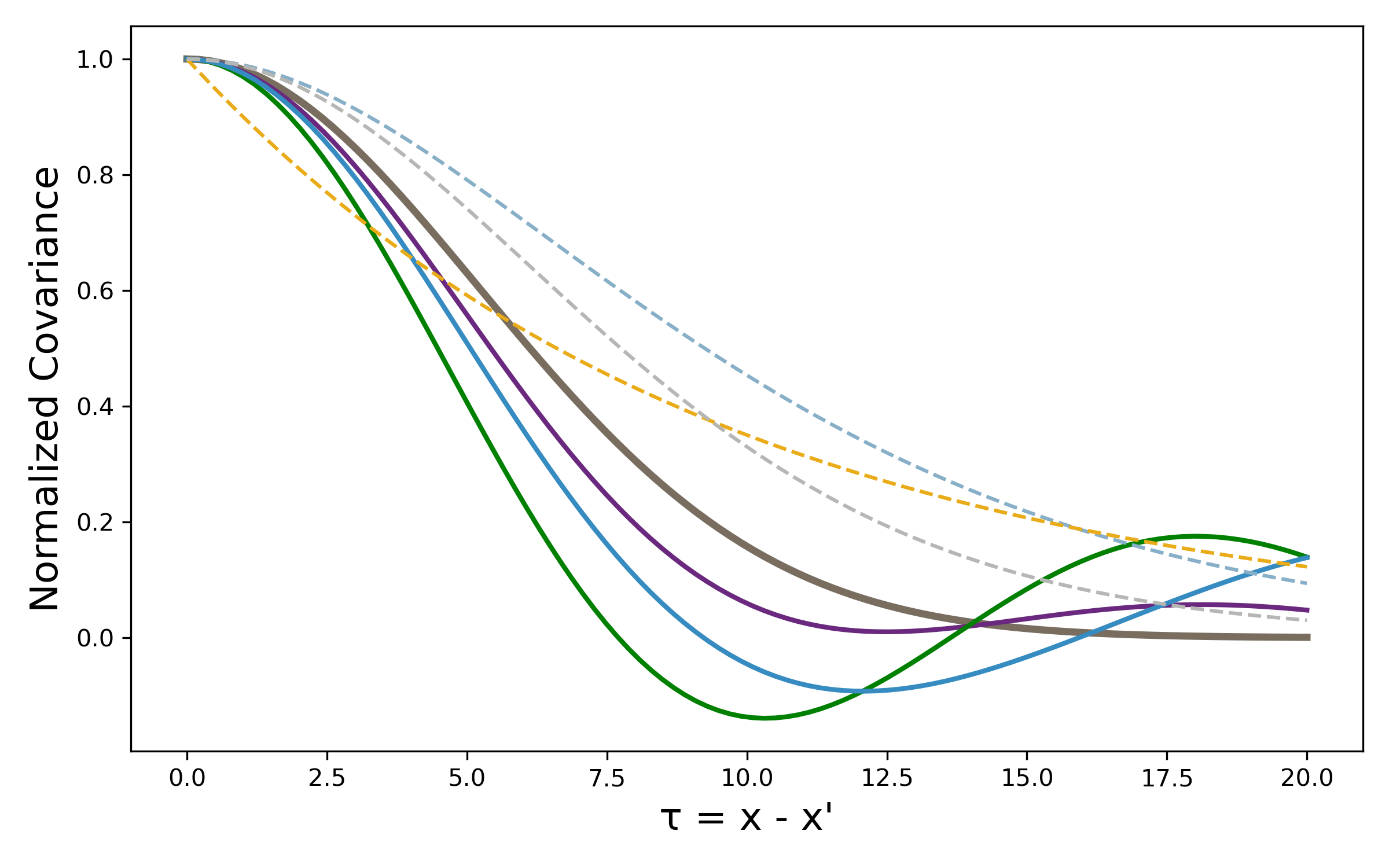
(a) SE

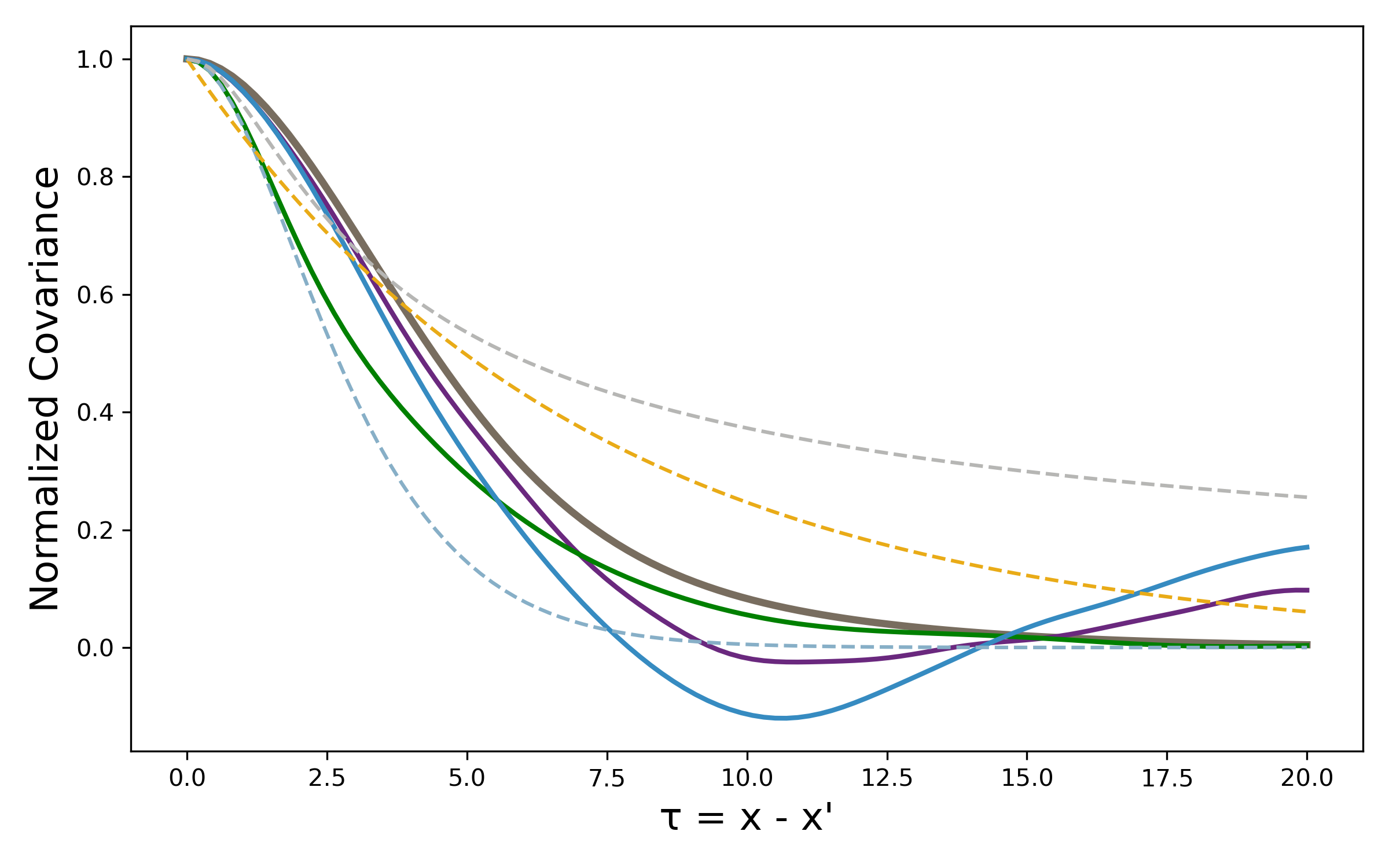
(b) SE+MA32

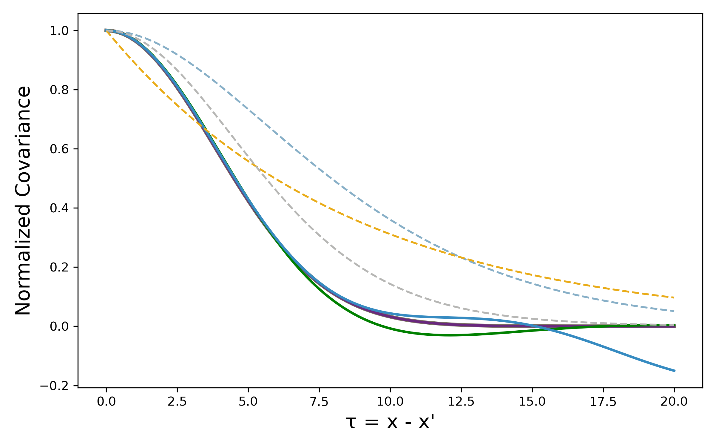
(c) SE*SE

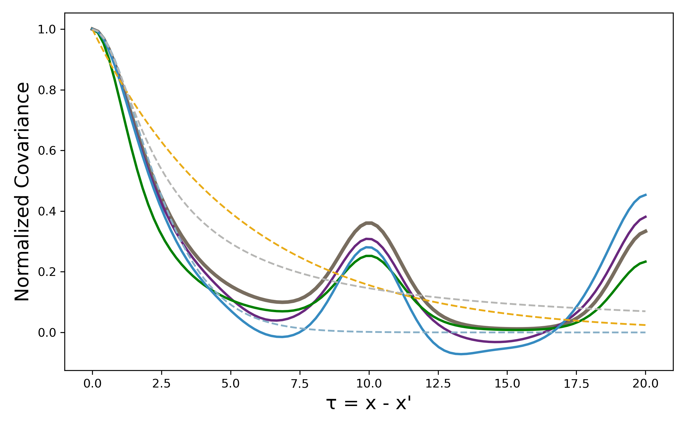
(f) PE+SE+MA32

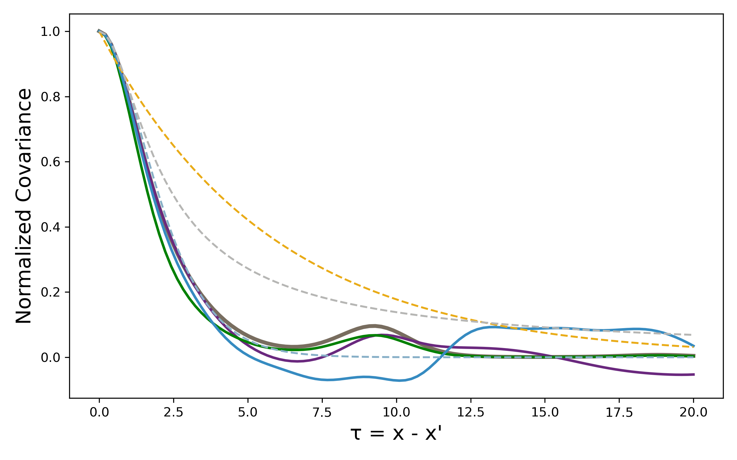
(d) SE*(PE+MA32)

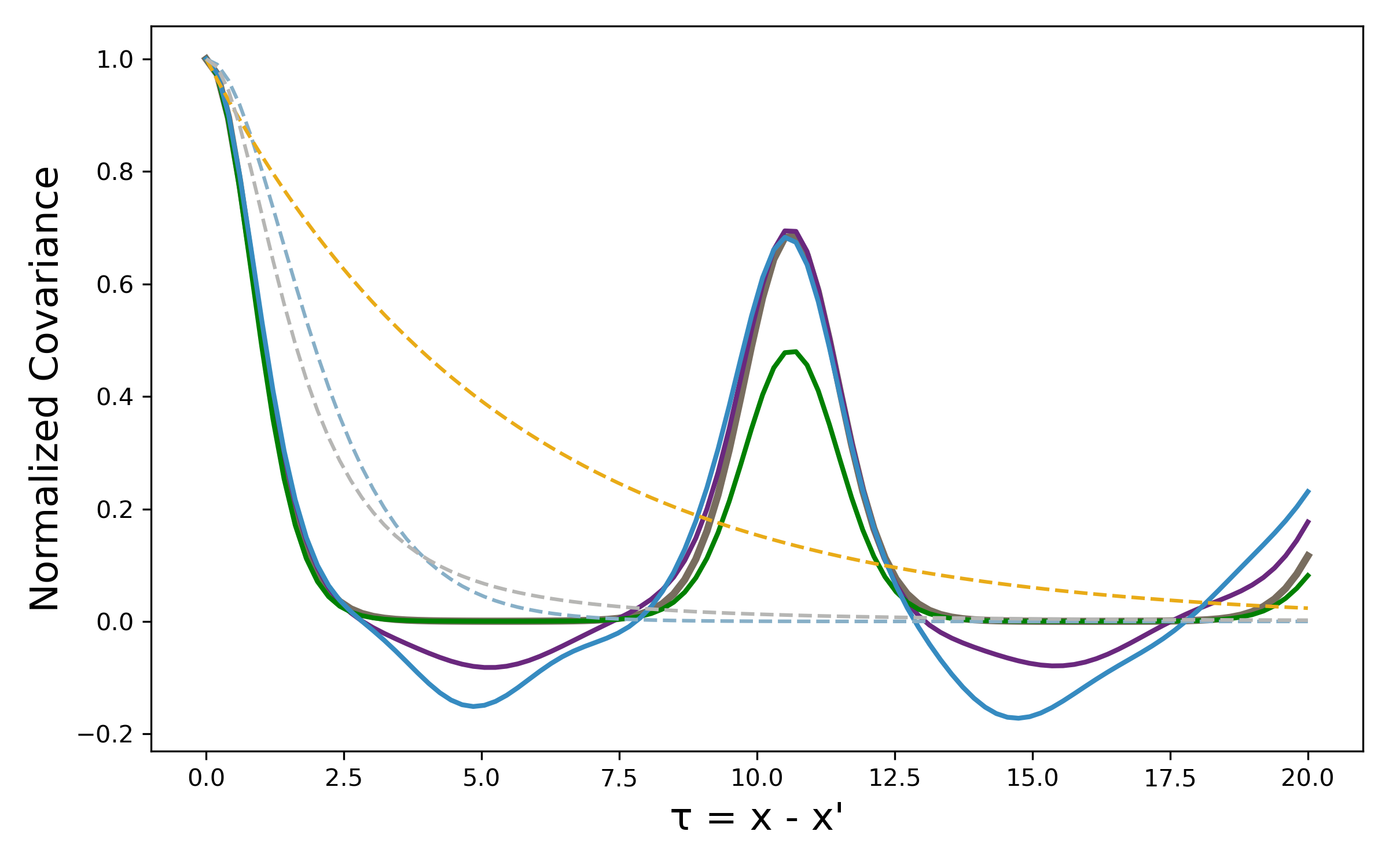
(e) PE*(SE+MA32)

Figure 2: Learned correlation function in kernel approximation. The horizontal axis denotes the Euclidean distance between two points, while the vertical axis represents the corresponding covariance distance. The darker solid line denotes the kernel that generates sampling points. Spectral mixture kernels more closely approximate the true kernel.

6.2 Optimization Performance

In this section, we validate our approach against several baselines across different optimization tasks. We implement BO with CSM, GSM, and CSM+GSM, and consider three sets of baseline models:

• Off-the-shelf BO implementations: SE, RQ, and MA52 kernels;

• Advanced BO methods: automatic Bayesian optimization (ABO) Malkomes_2018 and Adaptive Kernel Selection (ADA) Roman_2019_ADA ;

• Other spectral kernels: spectral Delta kernel (SDK) Vargas_2021_SDK and SINC kernel (SINC) Tobar_2019_SINC .

We consider a wider range of optimization problems with increasing dimensionality and complexity:

• Synthetic problems: Branin-2d, Hartmann-3d, Exponential-5d, Hartmann-6d, Exponential-10d, Rosenbrock-20d, Levy-30d;

• Real-world problems: Robot pushing-4d, Portfolio optimization-5d.

Details of our test functions, computational setup, and additional results are provided in Appendix C. The code is available at https://anonymous.4open.science/r/SpectralBO-0FE3/.

Figure 3 illustrates the performance of different methods across various optimization tasks using UCB acquisition function. In nearly all experiments, our method consistently outperforms existing baselines in both low- and high-dimensional settings, achieving an increase of over 11% in relative improvement, and a reduction of 76% in optimality gap. We also provide a summarized result in Table 4. To further validate the robustness of our method, we extended our evaluation to include EI and PI acquisition functions, as shown in Figures 5 and 6. The results confirm that our method maintains its performance advantage across different acquisition functions and problem settings.

To assess sensitivity to model complexity, we conduct an extensive ablation study evaluating $Q\in\{3,5,7,9\}$ components. As shown in Figure 7. We find that the results remain relatively stable across different mixture components, especially in higher-dimensional problems, with CSM+GSM demonstrating superior performance.

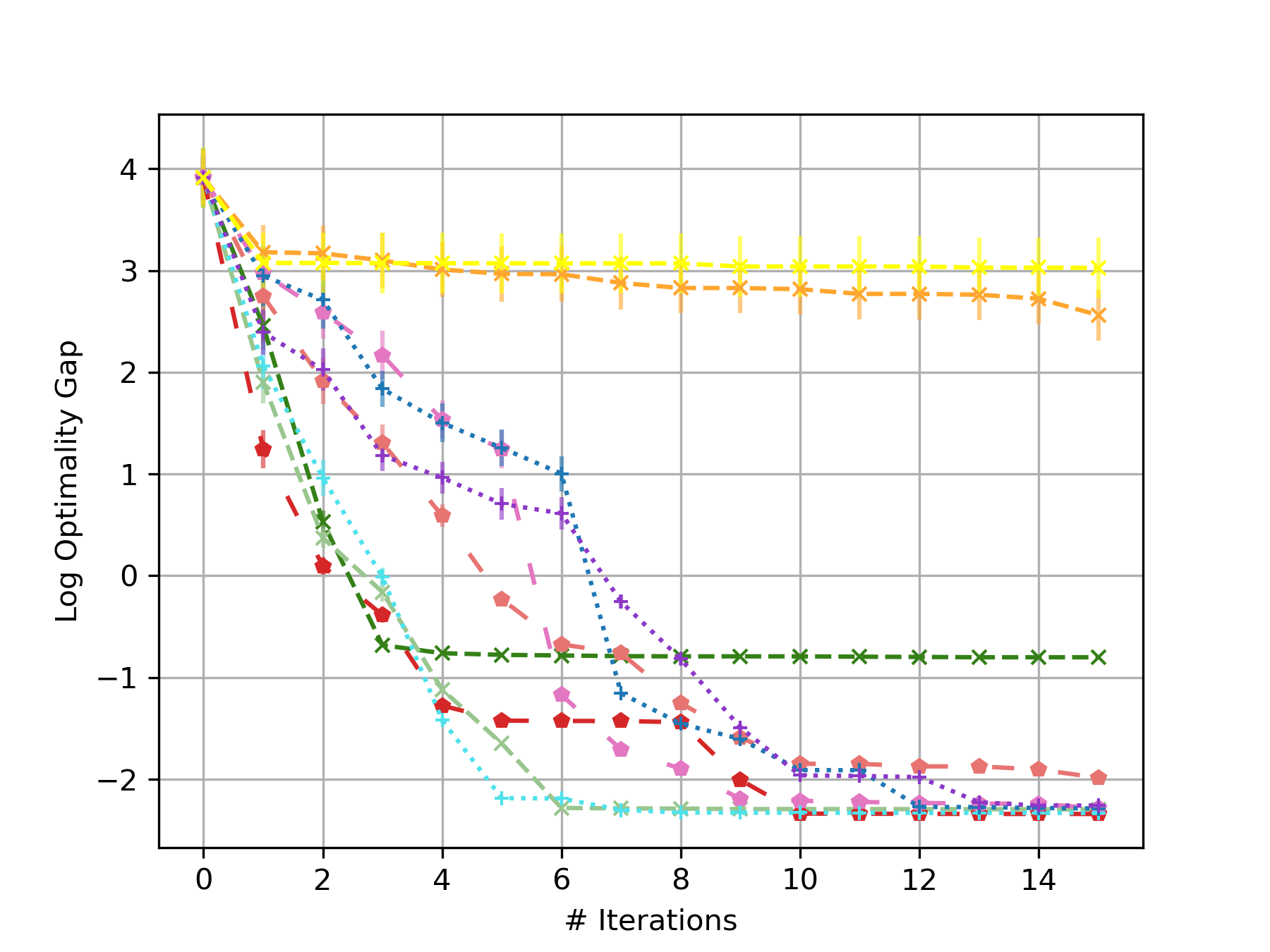
(a) Branin-2d

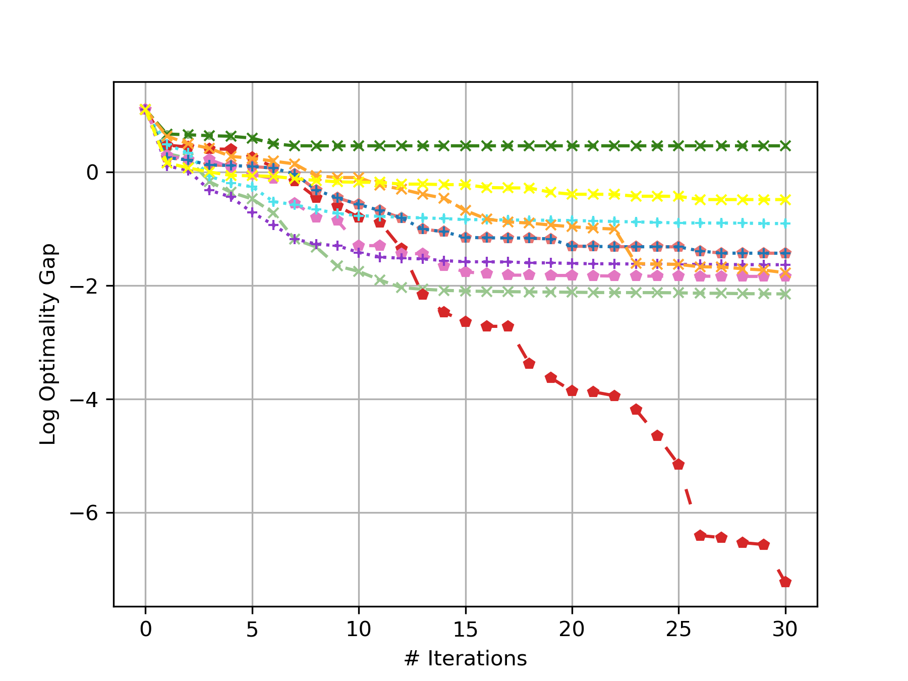
(b) Hartmann-3d

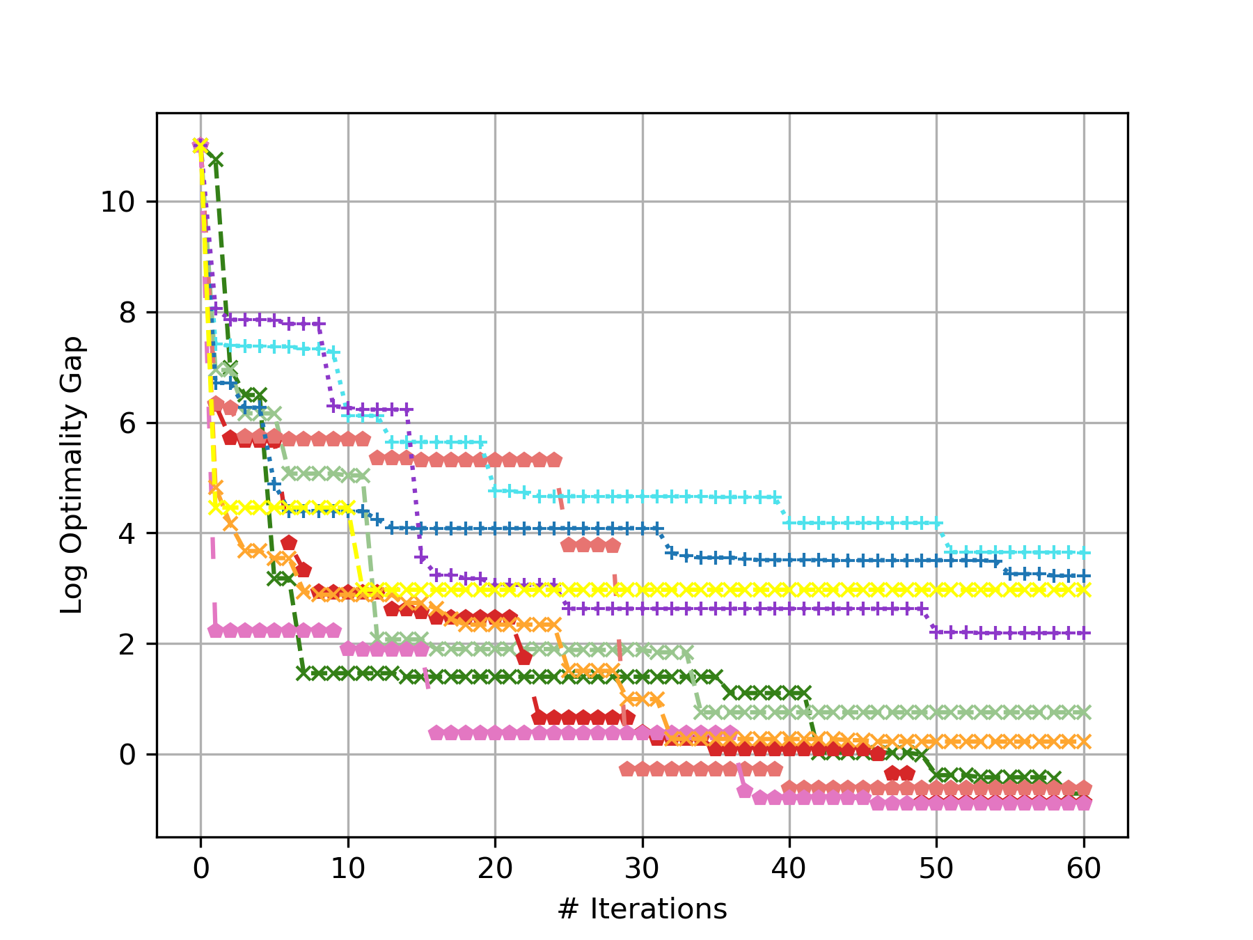
(c) Exponential-5d

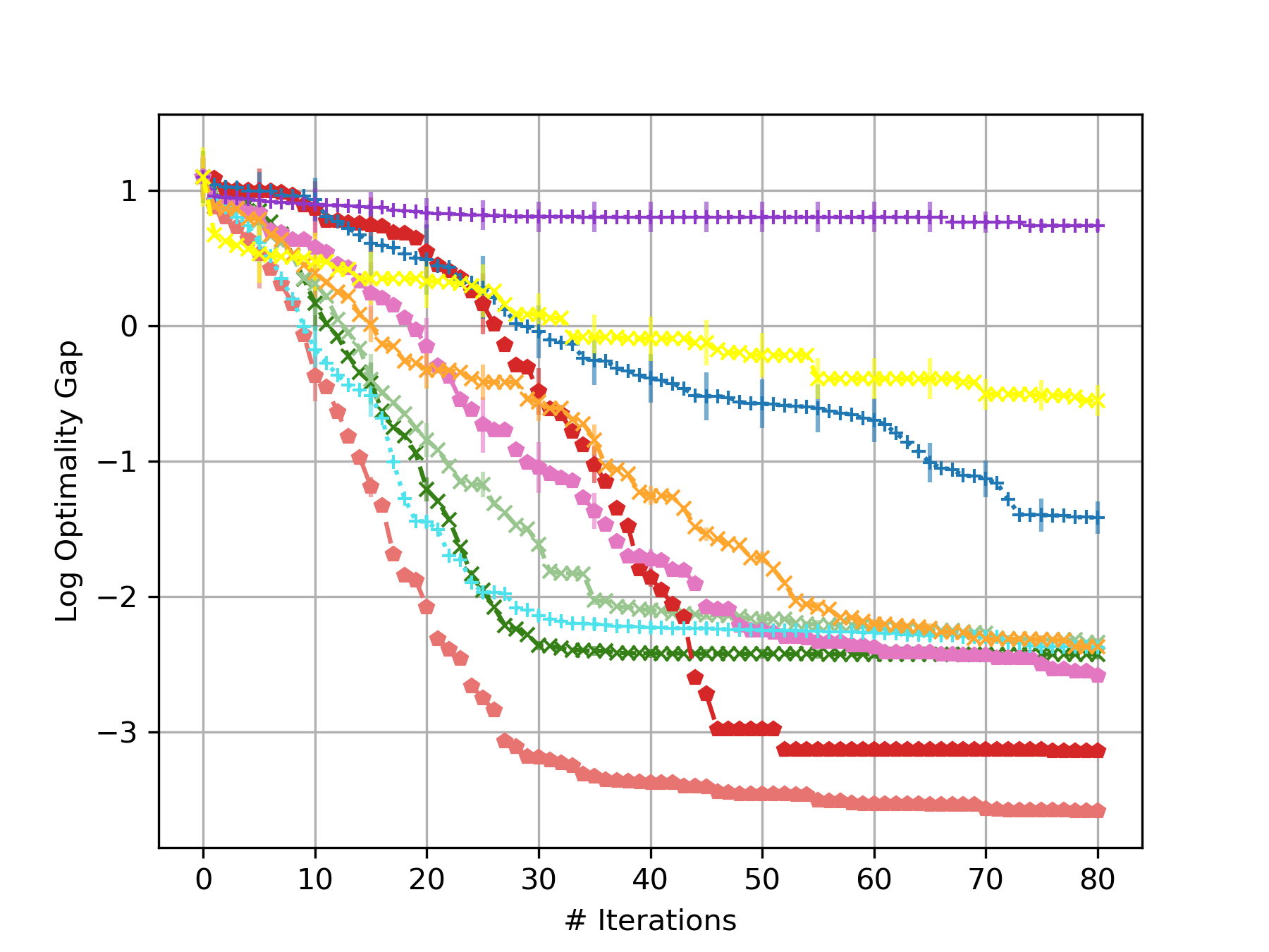
(d) Hartmann-6d

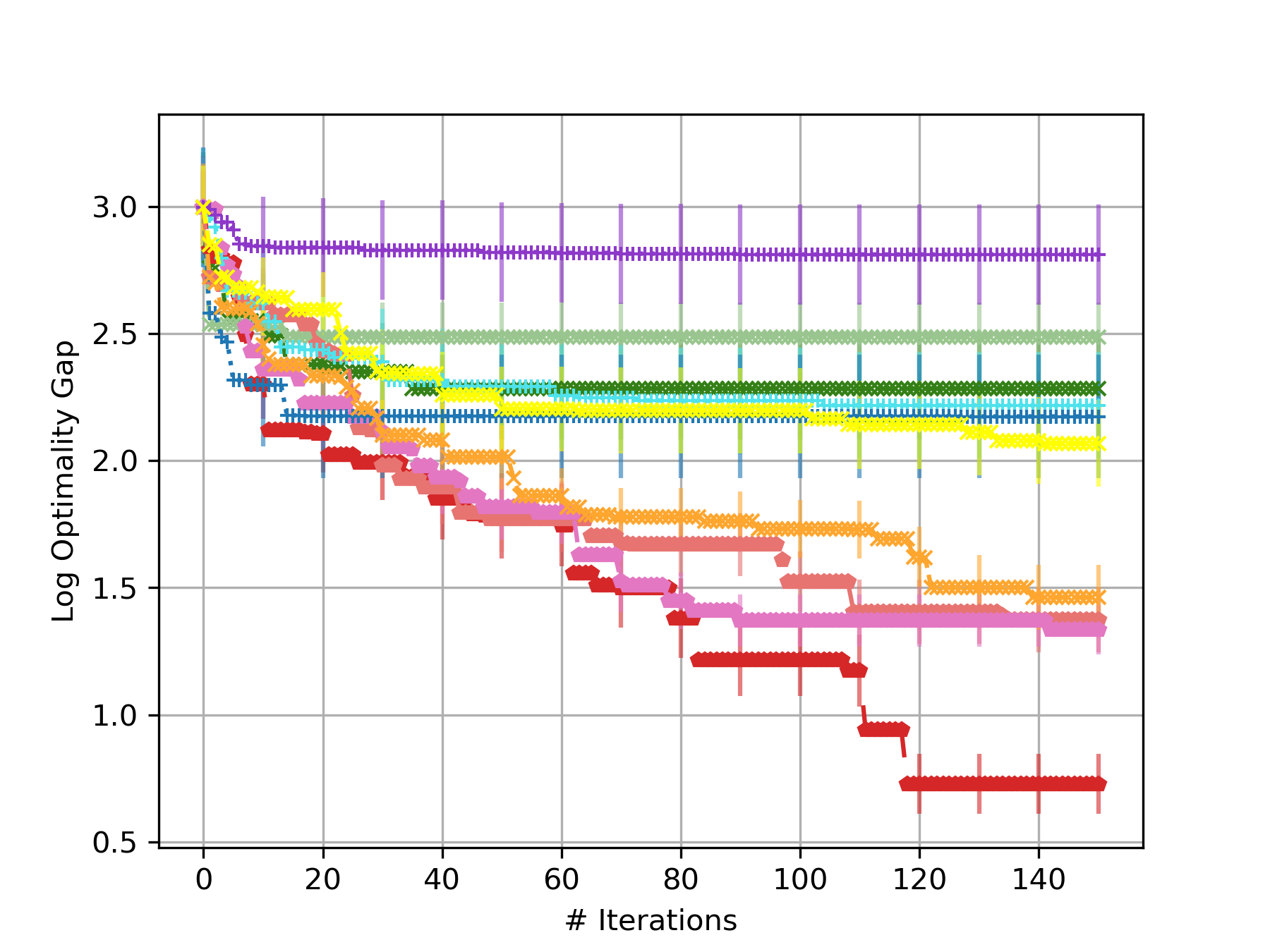
(e) Exponential-10d

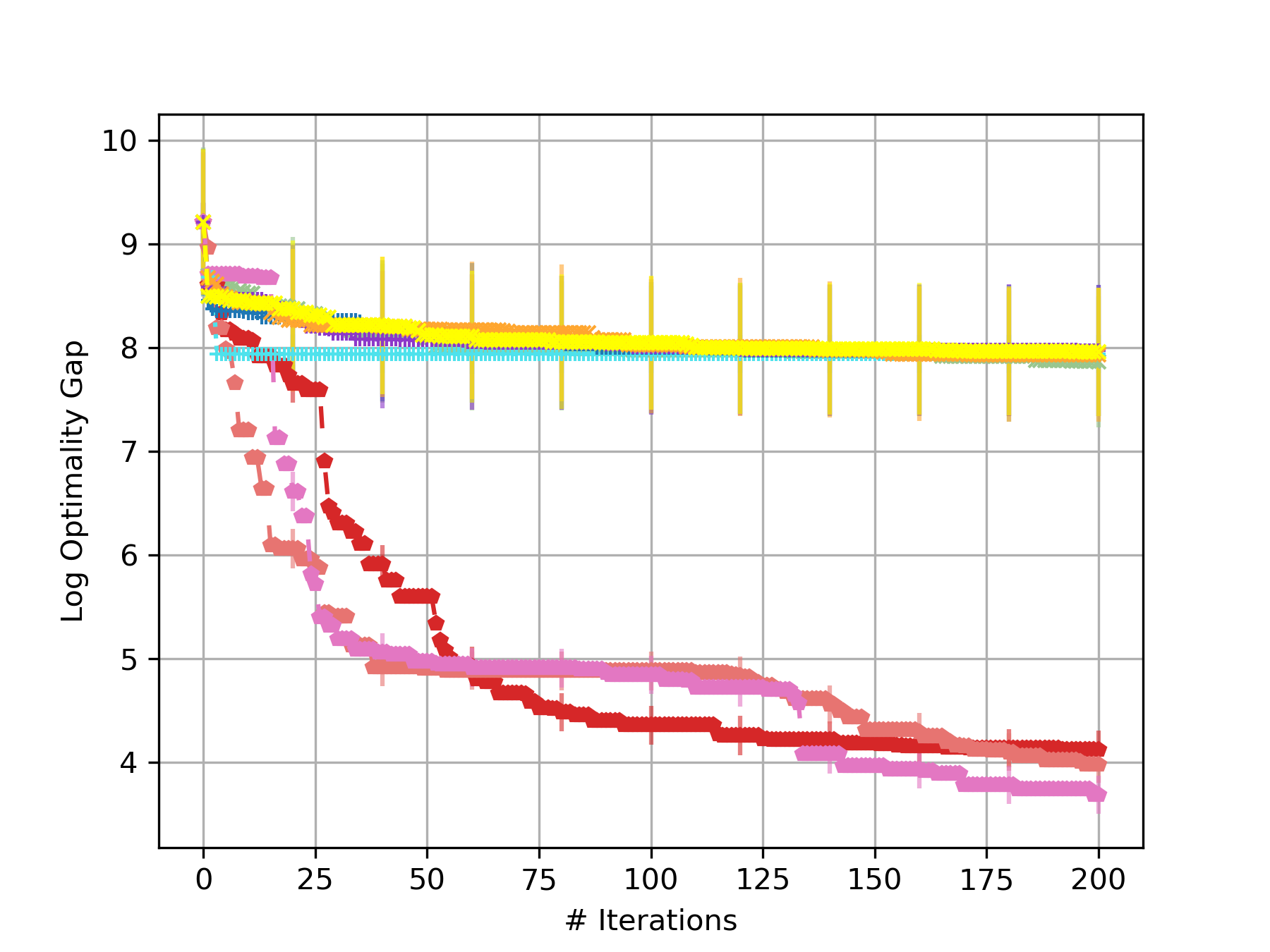
(f) Rosenbrock-20d

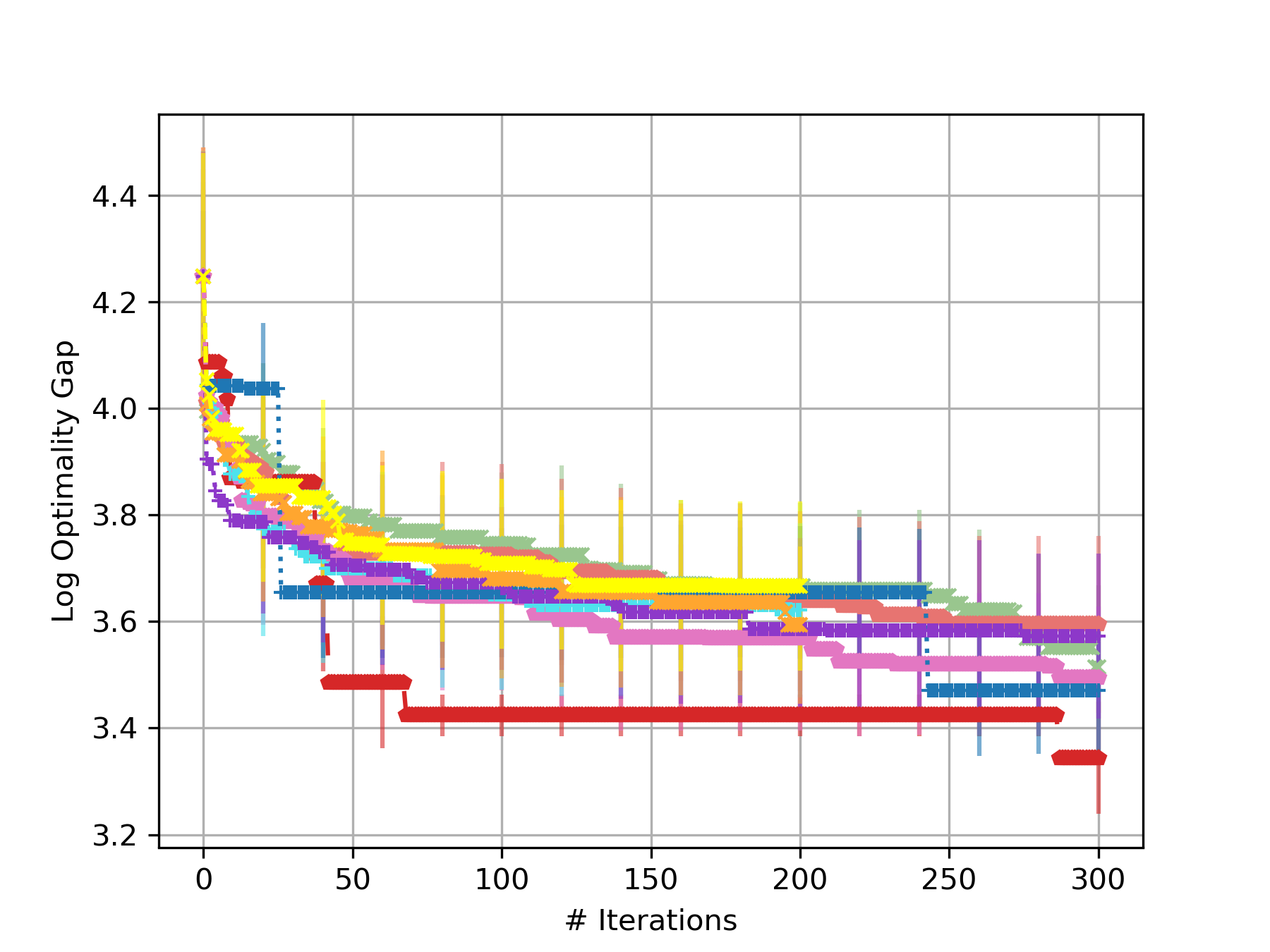
(g) Levy-30d

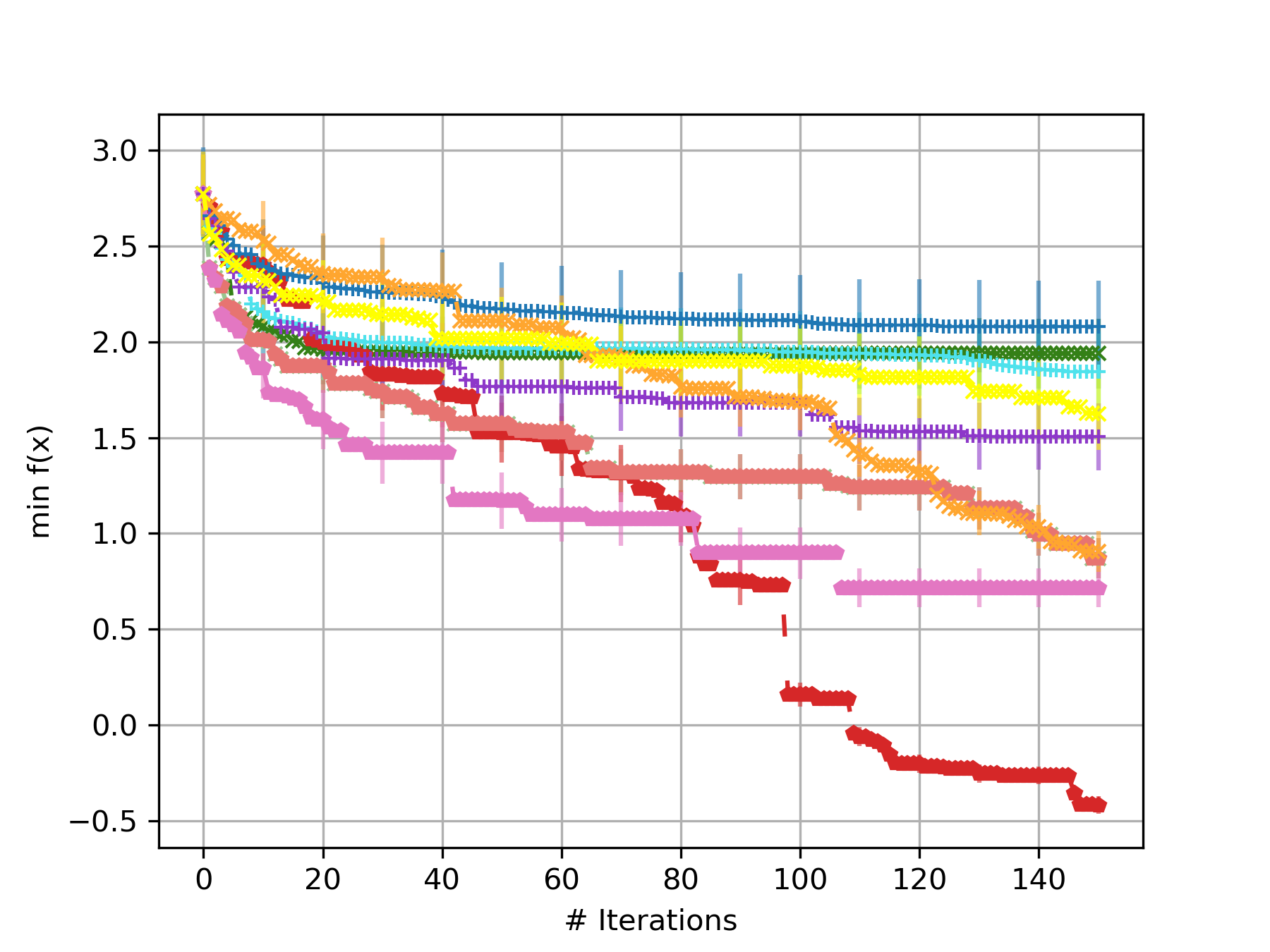
(h) Robot-4d

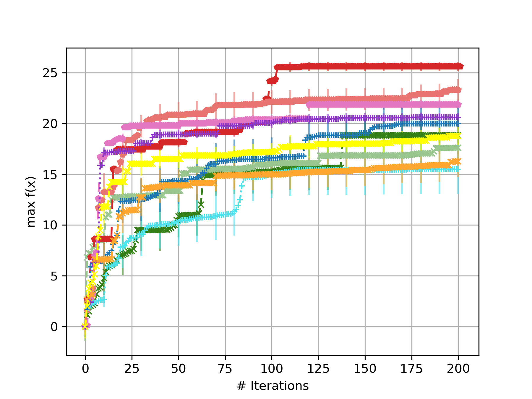
(i) Portfolio-5d

Figure 3: Performance of different test functions and algorithms across 10 repetitions using UCB acquisition function.

7 Conclusion and Future Work

We propose a new GP-based BO approach with spectral mixture kernels in the Fourier domain, which are derived by modeling a spectral density using mixtures of Cauchy and Gaussian distributions. We also provide bounds on the information gain and cumulative regret associated with obtaining the optimum. We empirically show that spectral mixture kernels with different densities can approximate a wide range of stationary kernels, which boosts the flexibility of GP and results in superior performance over existing conventional kernel methods.

This work represents an initial step in exploring BO methods using kernels in the Fourier domain. Future research could expand on this by exploring different forms of spectral mixture kernels, incorporating more mixture components, or considering other distribution families. Additionally, approximation techniques could be applied to spectral densities that are difficult to integrate. It would also be valuable to further investigate the performance of this approach in more complex settings, such as high-dimensional or constrained optimization problems.

Appendix A Primer on BO and GP

A.1 Bayesian Optimization

Consider the problem of minimizing an unknown, expensive-to-evaluate function $f$, which can be formulated as:

$$x^{*}=\arg\min_{x\in\mathcal{X}}f(x)$$

where $\mathcal{X}\subset\mathbb{R}^{d}$ denotes the search/decision space of interest and $x^{*}$ represents the global minimum. Starting with a limited set of observations, BO builds a probabilistic surrogate model, typically a GP, to estimate the unknown objective function. It then uses an acquisition function to evaluate and prioritize candidate solutions based on the model’s posterior distribution. The acquisition function guides the search by selecting the most promising points to evaluate next. After each new evaluation, the surrogate model is updated, and the process continues to refine the search. The method seeks to identify the optimal solution within the given constraints.

Algorithm 1 demonstrates the pseudo-code for BO with spectral mixture kernels using Upper Confidence Bound (UCB) as the acquisition function.

Algorithm 1 BO with Spectral Mixture Kernels

 Input: number of initial points $n_{0}$, spectral density $S$, iterations $N$

 Place a Gaussian process prior on $f$, with the kernel given by $\mathcal{F}(S)$

 Observe $f$ at $n_{0}$ points

 $n_{0}\rightarrow n$

 while $n\leq N$ do

  Update the posterior distribution on $f$ using all available data

  $x_{n+1}=\mathop{\arg\max}\limits_{x}\left(\mu(x)+\beta\sigma(x)\right)$

  Observe $y_{n+1}=f(x_{n+1})$

  Increment $n$

 end while

 Return a solution: either the point evaluated with the largest $f(x)$, or the point with the largest posterior mean

A.2 Gaussian Process

Gaussian process defines a distribution over functions $f:\mathcal{X}\rightarrow\mathbb{R}$, parameterized by a mean function $m(\cdot)$ and a covariance function $k(\cdot,\cdot)$:

$$f\sim\mathcal{GP}(m(x),k(x,x^{\prime})),$$

where $x\in\mathcal{X}$ is an arbitrary input variable, and the mean function $m(x)$ and covariance function $k(x,x^{\prime})$ are defined as

$$m(x)=\mathbb{E}[f(x)],\quad k(x,x^{\prime})=\operatorname{cov}(f(x),f(x^{\prime})).$$

For any finite set $\{x_{1},\ldots,x_{n}\}\subset\mathcal{X}$, the function values $f=(f(x_{1}),f(x_{2}),\ldots,f(x_{n}))$ follow a multivariate Gaussian distribution:

$$(f(x_{1}),f(x_{2}),\ldots,f(x_{n}))^{\top}\sim\mathcal{N}(\boldsymbol{\mu},\mathbf{K}),$$

where the $n\times n$ covariance matrix $\mathbf{K}$ has entries $K_{ij}=k(x_{i},x_{j})$, and the mean vector $\boldsymbol{\mu}$ has entries $\mu_{i}=m(x_{i})$. GP depends on specifying a kernel function, which measures the similarity between input points. A typical example is the SE kernel in Eq. (8). Functions drawn from a GP with this kernel are infinitely differentiable. Another example is the Matérn kernel with degrees of freedom $\nu=p+1/2$:

$$k_{\nu}(r)=e^{-\frac{\sqrt{2\nu}r}{\ell}}\frac{\Gamma(p+1)}{\Gamma(2p+1)}\sum_{i=0}^{p}\frac{(p+i)!}{i!(p-i)!}\left(\frac{\sqrt{8\nu}r}{\ell}\right)^{p-i},$$

which is $k$-times differentiable only if $k<\nu$.

A.3 Conventional Kernels

Squared Exponential, also known as Radial Basis Function (RBF):

$$k_{\text{SE}}(x,x^{\prime})=\exp(-\frac{\|x-x^{\prime}\|^{2}}{2\ell^{2}}),$$ (8)

Rational Quadratic:

$$k_{\text{RQ}}(\tau)=\left(1+\frac{\tau^{2}}{2\alpha\ell^{2}}\right)^{-\alpha},$$ (9)

Periodic:

$$k_{\text{PE}}(\tau)=\exp\left(-2\sin^{2}(\pi\tau\omega)/\ell^{2}\right).$$ (10)

Matérn kernel with $\nu=\frac{3}{2}$:

$$k_{\nu=3/2}(\tau)=\left(1+\frac{\sqrt{3}\tau}{\ell}\right)\exp\left(-\frac{\sqrt{3}\tau}{\ell}\right),$$ (11)

Matérn kernel with $\nu=\frac{5}{2}$:

$$k_{\nu=5/2}(\tau)=\left(1+\frac{\sqrt{5}\tau}{\ell}+\frac{5\tau^{2}}{3\ell^{2}}\right)\exp\left(-\frac{\sqrt{5}\tau}{\ell}\right).$$ (12)

We refer readers to Rasmussen & Williams [22] for a comprehensive catalog of different kernels.

Appendix B Technical Proofs

B.1 Proof of Theorem 4.1

Spectral density $S(s)$ of Cauchy distribution is given in Eq. (4), substituting it into Eq. (1):

$$k(\tau)=\int_{-\infty}^{\infty}\frac{1}{\pi\gamma\left[1+\left(\frac{s-x_{0}}{\gamma}\right)^{2}\right]}e^{2\pi is\tau}\,ds.$$

To simplify the integral, let:

$$u=\frac{s-x_{0}}{\gamma},\quad ds=\gamma du,\quad s=\gamma u+x_{0}.$$

We have

$$k(\tau) =\int_{-\infty}^{\infty}\frac{1}{\pi\gamma(1+u^{2})}e^{2\pi i(\gamma u+x_{0})\tau}\gamma du=\frac{1}{\pi}\int_{-\infty}^{\infty}\frac{e^{2\pi i\gamma u\tau}e^{2\pi ix_{0}\tau}}{1+u^{2}}du=e^{2\pi ix_{0}\tau}\frac{1}{\pi}\int_{-\infty}^{\infty}\frac{e^{2\pi i\gamma u\tau}}{1+u^{2}}du.$$

Next, we calculate the standard integral using contour integration:

$$I(\tau)=\int_{-\infty}^{\infty}\frac{e^{2\pi i\gamma u\tau}}{1+u^{2}}du.$$

where the integrand is:

$$f(u)=\frac{e^{2\pi i\gamma u\tau}}{1+u^{2}}.$$

We are interested in integrating this function along the real line. To apply contour integration, we extend the function to the complex plane. The function $\frac{1}{1+u^{2}}$ has simple poles at $u=i$ and $u=-i$. The residues at these poles are:

$$\text{Res}(f,i)=\lim_{u\to i}(u-i)\frac{e^{2\pi i\gamma u\tau}}{1+u^{2}}=\frac{e^{-2\pi\gamma\tau}}{2i},$$

$$\text{Res}(f,-i)=\lim_{u\to-i}(u+i)\frac{e^{2\pi i\gamma u\tau}}{1+u^{2}}=\frac{e^{2\pi\gamma\tau}}{-2i}.$$

We use the residue theorem, which states that the integral of a meromorphic function around a closed contour is $2\pi i$ times the sum of the residues inside the contour. By closing the contour in the upper half-plane (since $e^{2\pi i\gamma u\tau}$ decays for large $u$ in the upper half-plane), we get:

$$\int_{-\infty}^{\infty}\frac{e^{2\pi i\gamma u\tau}}{1+u^{2}}du=2\pi i\cdot\text{Res}(f,i).$$

Thus,

$$I(\tau)=\pi e^{-2\pi|\gamma\tau|}.$$

Substituting this result into the expression for $k(\tau)$, we get:

$$k(\tau) =exp(2\pi ix_{0}\tau)exp(-2\pi|\gamma\tau|)=[\cos(2\pi x_{0}\tau)+i\sin(2\pi x_{0}\tau)]\exp(-2\pi|\gamma\tau|).$$

Exploiting the symmetry of $S(s)$ gives

$$k(\tau)=\exp\left(-2\pi|\gamma\tau|\right)\cos(2\pi\tau x_{0}).$$

B.2 Proof of Theorem 5.1

We first state a theorem that gives an upper bound for information gain $\gamma(T)$ with a particular kernel $k$, given that $B_{k}(T_{*})$ is known.

Theorem B.1 (Srinivas et al. [27]).

Suppose that $D\subset\mathbb{R}^{d}$ is compact. Let $B_{k}(T_{*})=\sum_{s>T_{*}}\lambda_{h}$, where $\{\lambda_{h}\}$ is the operator spectrum of $k$ with respect to the uniform distribution over $D$. Pick $\tau>0$, and let $n_{T}=C_{4}T^{\tau}(\log T)$ with $C_{0}=2\mathcal{V}(D)(2\tau+1)$. Then, the following bound holds true:

$$\gamma(T)\leq \frac{1/2}{1-e^{-1}}\max_{r=1,\ldots,T}\left(T_{*}\log\left(\frac{rn_{T}}{\sigma^{2}}\right)+C_{0}\sigma^{-2}(1-r/T)(\log T)\left(T^{\tau+1}B_{k}(T_{*})+1\right)\right)$$

$$+\mathcal{O}(T^{1-\tau/d})$$

for any $T_{*}\in\{1,\ldots,n_{T}\}$.

To obtain the tail bound on $B_{k}(T_{*})=\sum_{h>T_{*}}\lambda_{h}$, we further draw on a theorem of Widom [35], which gives the asymptotic behavior of the operator spectrum $\{\lambda_{h}\}$.

Assumption B.2.

We assume that the covariate distribution $\mu$ has a bounded density, such that

$$\int I_{\{\|x\|\leq T\}}\mu(x)^{d/(2\nu+d)}\,dx\leq\tilde{C},$$

where $\tilde{C}$ is a constant independent of $T>0$.

Assumption B.2 provides a controlled growth of $\mu(x)$, ensuring that the covariates are not overly concentrated in any specific region, which could lead to numerical instabilities or biased estimation. Distributions that satisfy this assumption include uniform, Gaussian, and truncated power-law distributions, among others.

Theorem B.3 (Widom [35]).

Define

$$\psi(\varepsilon)=(2\pi)^{-d}\int I_{\{\mu(x)S(s)>(2\pi)^{-d}\varepsilon\}}\,dx\,d\omega,$$ (13)

where $S(s)$ is the spectral density and $h=h(\varepsilon)=\min\{h^{\prime}\mid\lambda_{h^{\prime}}>\varepsilon\}$. we have

$$\psi(\varepsilon)\sim h(\varepsilon),\quad\varepsilon\to 0.$$

where both $\psi(\varepsilon)$ and $h(\varepsilon)$ are non-increasing and $h(\varepsilon)$ is unbounded as $\varepsilon\to 0$.

When $\psi(\varepsilon)$ is strictly decreasing and $\psi^{-1}(h+o(h))\sim\psi^{-1}(h)$ for $h\to\infty$. The asymptotic distribution of eigenvalues $\lambda_{h}$ satisfies

$$\lambda_{h}\sim\psi^{-1}(h),\quad h\to\infty.$$

Theorem B.1 gives a upper bound on $\gamma(T)$, provided that $B_{k}(T_{*})=\sum_{h>T_{*}}\lambda_{h}$ is known. Theorem B.3 gives the asymptotic behavior of $\lambda_{h}$, so we can compute $B_{k}(T_{*})$. Following this path, we first show how $\lambda_{h}$ is derived.

Lemma B.4.

Let $K(\tau)$ be the CSM kernel with $d$-dimensioanl inputs. Define the bounded support measure $\mu_{T}$ with density $\mu_{T}(x)=I_{\{\|x\|\leq T\}}\mu(x)$, and let $\{\lambda_{h}\}$ be the spectrum of $K(\tau)$ w.r.t. $\mu_{T}$. Then, for all $T>0$ large enough, there exists a $h_{0}$ such that

$$\lambda_{h}\leq Ch^{-(d+1)/d}\quad\forall h\geq h_{0}.$$

Here, $C$ is a constant independent of $T$.

Proof.

The joint distribution of $d$ independent standard Cauchy is given by

$$\lambda(\eta)=\frac{\Gamma\left(\frac{d+1}{2}\right)}{\pi^{\frac{d+1}{2}}}\cdot\frac{1}{\left(1+||\eta||^{2}\right)^{\frac{d+1}{2}}}.$$

To upper bound Eq. (13) for the measure $\mu_{T}$, we first transform $\psi_{T}(\varepsilon)$ into polar coordinates. Recall that $d\omega=A^{d-1}\eta^{d-1}d\eta d\sigma$ with $d\sigma$ the uniform distribution on the unit sphere, and $A^{d-1}=2\pi^{d/2}/\Gamma(d/2)$. If $y=1+||\eta||^{2},q=(d+1)/2$, then

$$\psi_{T}(\varepsilon)=C_{1}\int_{0}^{\infty}\int_{\|x\|\leq T}I_{\{y^{-q}\mu(x)>c_{1}\varepsilon\}}\eta^{d-1}\,dx\,d\eta,$$ (14)

where

$$C_{1}=\frac{2^{1-d}\pi^{-d/2}}{\Gamma(d/2)},\quad c_{1}=\pi.$$

Let $\rho=(c_{1}\varepsilon)^{-1}$. Note that $\rho\to\infty$ as $\varepsilon\to 0$. Now,

$$\eta^{d-1}(d\eta)=\frac{1}{2}(y-1)^{\frac{d}{2}-1}\,dy,$$

so that

$$\psi_{T}(\varepsilon)=C_{2}\int_{\|x\|\leq T}\int_{1}^{\infty}I_{\{y^{q}<\rho\mu(x)\}}G(y)\,dy\,dx$$ (15)

with $C_{2}=\frac{1}{2}C_{1},G(y)=(y-1)^{\frac{d}{2}-1}$. Integrating out $y$, we have that

$$\psi_{T}(\varepsilon)\sim C_{2}\frac{2}{d}\rho^{\frac{d}{2q}}\int I_{\{\|x\|\leq T\}}\mu(x)^{\frac{d}{2q}}\,dx.$$

The integration leaves us with $(\rho\mu(x))^{1/q}-1)^{2/d}$. We can use the binomial theorem in order to write that as a polynomial in $(\rho\mu(x))^{1/q}$, which is dominated by the highest degree term as $\varepsilon\to 0$. Moreover, since $(y-1)^{2/d}\leq y^{2/d}$ for $y\geq 1$, the right-hand side is also an exact upper bound once $\rho\geq\rho_{0}:=\sup\{\mu(x)^{-1}\mid\|x\|\leq T\}$. Note that $q=(d+1)/2$ If $C_{3}=C_{2}\frac{2}{d}\tilde{C}c_{1}^{-2q/d}$, then $\psi_{T}(\varepsilon)\leq C_{3}(1+o(1))\varepsilon^{-2q/d}$ as $\varepsilon\to 0$. Widom’s theorem gives that $s-1\leq C_{3}(1+o(1))(\lambda_{h})^{-d/2q}$. The lemma follows by solving for $\lambda_{h}$. ∎

Therefore, $B_{k}(T_{*})=\sum_{h>T_{*}}=\mathcal{O}\left(T_{*}^{1-(d+1)/d}\right)$. Following Srinivas et al. [27], we choose $T_{*}=(Tn_{T})^{d/(1+d)}(\log(Tn_{T}))^{-(1+d)/d}$, so that the upper bound $\gamma(T)$ becomes:

$$\max_{r=1,\ldots,T}\left(T_{*}\log\left(\frac{rn_{T}}{\sigma^{2}}\right)+\sigma^{-2}(1-r/T)\times\left(C_{3}T_{*}(\log(Tn_{T}))+C_{0}(\log T)\right)\right)+\mathcal{O}(T^{1-\tau/d})$$

with $n_{T}=C_{0}T^{\tau}(\log T)$. The maximum of upper bound $\gamma(T)$ over $r$ is $\mathcal{O}(T_{*}\log(Tn_{T}))=\mathcal{O}(T^{(\tau+1)d/(d+1)}(\log T))$. Next, we choose $\tau=d/(d^{2}+d+1)$ to match this term with $\mathcal{O}(T^{1-\tau/d})$. Plugging this in, we can obtain $\gamma(T)$.

Lemma B.5.

Let $K(\tau)$ be the GSM kernel with $d$-dimensional inputs. Then, for all $T>0$ large enough, there exists a $h_{0}$ such that

$$\lambda_{h}\leq C\cdot B^{h^{1/d}}\quad\forall h\geq h_{0}.$$

where $B<1$, $C$ is a constant independent of $T$.

Proof.

The joint distribution of $d$ independent standard Gaussian distributions is given by

$$\lambda(\eta)=\frac{1}{(\sqrt{2\pi})^{d}}\exp(-\frac{||\eta||^{2}}{2})$$

For covariate distributions $\mu(x)$ that satisfy Assumption B.2, the same decay rate holds for $\lambda_{h}$, while the constants might change [27]. Therefore, without loss of generality, we assume $\mu(x)=N(x|0,\boldsymbol{I})$. In this case, the eigenexpansion of $k$ is known explicitly for $d=1$ [40]:

$$\lambda_{h}=(\frac{1}{2A})^{1/2+h},\quad A=\frac{1}{4}+\frac{1}{2}+\sqrt{\frac{5}{16}}.$$

Following the analysis of Seeger et al [25], in cases where $d>1$, a tight bound can be obtained on $\lambda_{h}$:

$$\lambda_{h}\leq(\frac{1}{2A})^{d/2}(B)^{h^{1/d}}$$

where $B<1$, $A$ is a constant independent of $T$.

Because the same decay rate holds for any $\mu(x)$ satisfying Assumption B.2. The lemma follows by keeping the decay rate $B^{h^{1/d}}$ while changing the constant term. ∎

Upper bound on information gain w.r.t $\lambda_{h}$ satisfying Lemma B.5 is given in Srinivas et al. [27]. This completes our proof for Theorem 5.1.

Appendix C Experiments

C.1 Implementation Details

Approximation

To further validate the flexibility of our proposed spectral mixture kernel, we considered the approximation of more sophisticated conventional kernels. The parameters for source kernels that generate the data are shown in Table 2.

Table 2: Parameters for source kernels generating the training data. The lengthscale and outputscale parameters are the same for all MA52, MA32, and PE.

Parameters	Value
number of data	80
number of repetitions	10
number of mixture	10
lengthscale	5
outputscale	4
period	10

Optimization

The objective is to identify the global optimum of each test function within a limited number of evaluations. We optimize each acquisition function using the LBFGS method [39]. We conduct 10 trials for all problems. Mean and standard errors are reported in all cases. All models employ UCB as the acquisition function. The kernel hyperparameters, as well as the observation noise, are inferred via marginal likelihood maximization after each function evaluation.

Performance Metric

For portfolio optimization tasks, we directly evaluate performance using investment returns. For other optimization problems, we employ the log-optimality gap metric:

$$gap=\log(|f_{n}^{*}-f_{\text{opt}}|),$$

where $f_{n}^{*}$ is the optimal solution found by the model, and $f_{\text{opt}}$ is the true global optimum.

To quantify algorithmic improvements, we introduce two comparative metrics.

Relative improvement increase:

$$\frac{(RI_{\text{spectral}}-RI_{\text{baseline}})}{RI_{\text{baseline}}},\quad RI=\frac{f_{n}^{*}-f_{0}}{f_{\text{opt}}-f_{0}};$$

Optimality gap reduction:

$$\frac{(OG_{\text{baseline}}-OG_{\text{spectral}})}{OG_{\text{baseline}}},\quad OG=f_{n}^{*}-f_{\text{opt}}.$$

Computational Resources

All experiments were performed on an Ubuntu 20.04 server equipped with an AMD Ryzen 9 5950X CPU (16 cores, 32 threads), 125 GiB RAM, and an NVIDIA RTX 3090 GPU (24 GiB VRAM). The primary storage was a 1.8 TB NVMe SSD.

C.2 Test Functions

C.2.1 Synthetic Functions

Our first set of experiments involves test functions commonly used for optimization. The hyperparameters to be optimized are summarized in Table 3.

C.2.2 Simulated Problems

Robot Pushing

We consider a Robot Pushing problem widely used in recent literature [10, 16, 18]. This problem addresses an active learning task for the pre-image learning problem in robotic pushing. The goal is to determine an optimal pre-image for pushing the robot to a desired location, with the pushing action as the input and the distance from the goal location as the output. We test a 4-dimensional input function: robot location $(r_{x},r_{y},r_{\theta})$, and pushing duration $t_{r}$.

Portfolio Optimization

Another real-world problem is portfolio optimization. Our goal is to tune the hyperparameters of a trading strategy so as to maximize investment return. We simulate and optimize the evolution of a portfolio over a period of four years using open-source market data.

Since the simulator CVXPortfolio [3] is expensive to evaluate, with each evaluation taking around 3 minutes, evaluating the performance of the various algorithms becomes prohibitively expensive. Therefore, following Cakmak et al. [4], we do not use the simulator directly in the experiments. Instead, we build a surrogate function obtained as the mean function of a GP trained using evaluations of the actual simulator across 3000 points chosen according to a Sobol sampling design [19].

Table 3: Test functions used in our experiments. The analytic form of synthetic test functions, as well as the global minima, are available in [29].

Objective Function	Type	Dimension	Iterations	Input Domain
Branin	min	2	15	$x\in[-3,3]^{2}$
Hartmann	min	3	30	$x\in[0,1]^{3}$
Exponential	min	5	60	$x\in[-5.12,5.12]^{5}$
Hartmann	min	6	80	$x\in[0,1]^{6}$
Exponential	min	10	150	$x\in[-5.12,5.12]^{10}$
Rosenbrock	min	20	200	$x\in[-2.048,2.048]^{20}$
Levy	min	30	200	$x\in[-5,5]^{30}$
Robot Pushing	min	4	150	$x_{0}\in[-5,5]$ ($x$-position), $x_{1}\in[-5,5]$ ($y$-position), $x_{2}\in[1,30]$ (pushing duration), $x_{3}\in[0,2\pi]$ (pushing angle),
Portfolio	max	5	200	$x_{0}\in[0.1,1000]$ (risk parameter), $x_{1}\in[5.5,8.0]$ (trade aversion parameter), $x_{2}\in[0.1,100]$ (holding cost multiplier), $x_{3}\in[10^{-4},10^{-2}]$ (bid-ask spread), $x_{4}\in[10^{-4},10^{-3}]$ (borrow cost)

C.3 Result Analysis

For synthetic problems, the results indicate that both CSM and GSM outperform other methods in terms of convergence and optimality gap. Notably, CSM+GSM demonstrates superior performance across most baseline functions. This performance advantage grows with the dimensionality of the problem. For the conventional kernels, performance varies significantly depending on the task. Specifically, single kernels perform as good on Branin-2d, a simple, low-dimensional problem where all methods show similar performance.

As we transition to more practical objective functions, the advantages of a more flexible and computationally efficient model become clear. Each type of spectral mixture kernel outperforms all other methods, with the one using both Gaussian and Cauchy components delivering the best performance. As a result, the log optimality gap is nearly two orders of magnitude smaller compared to standard BO methods using conventional kernels.

Table 4: Results for different test functions and algorithms across 10 repetitions using UCB acquisition function. In each cell, the first number represents the mean results, and the second number (inside parentheses) indicates the standard error. ABO failed in Rosenbrock-20d and Levy-30d.

Objective	Dim	RBF	RQ	MA52	ABO	ADA	SDK	SINC	CSM	GSM	CSM+GSM
Branin	2	-2.29 (0.02)	-2.25 (0.03)	-2.33 (0.02)	-0.80 (0.03)	-2.29 (0.01)	2.56 (0.15)	3.02 (0.08)	-1.98 (0.03)	-2.29 (0.03)	-2.34 (0.01)
Hartmann	3	-1.43 (0.06)	-1.63 (0.05)	-0.91 (0.10)	0.46 (0.15)	-2.14 (0.11)	-1.77 (0.07)	-0.49 (0.06)	-3.21 (0.10)	-1.84 (0.12)	-7.22 (0.20)
Exponential	5	3.23 (0.05)	2.19 (0.09)	3.64 (0.06)	-0.71 (0.13)	0.76 (0.07)	0.23 (0.04)	2.97 (0.10)	-0.61 (0.14)	-0.89 (0.09)	-0.87 (0.06)
Hartmann	6	-1.41 (0.08)	0.74 (0.09)	-2.36 (0.12)	-2.43 (0.15)	-2.34 (0.10)	-2.36 (0.08)	-0.55 (0.06)	-3.14 (0.12)	-2.59 (0.13)	-3.14 (0.15)
Exponential	10	2.17 (0.14)	2.81 (0.16)	2.21 (0.14)	2.28 (0.13)	2.48 (0.19)	1.46 (0.13)	2.06 (0.16)	1.37 (0.18)	1.33 (0.17)	0.72 (0.18)
Rosenbrock	20	7.97 (0.42)	7.97 (0.46)	7.94 (0.45)	–	7.86 (0.45)	7.93 (0.47)	7.96 (0.46)	3.97 (0.40)	3.68 (0.38)	4.11 (0.39)
Levy	30	3.47 (0.28)	3.57 (0.24)	3.62 (0.25)	–	3.51 (0.27)	3.59 (0.27)	3.66 (0.23)	3.59 (0.22)	3.49 (0.25)	3.34 (0.21)
Robot	4	2.08 (0.05)	1.51 (0.06)	1.84 (0.07)	1.94 (0.05)	0.87 (0.04)	0.91 (0.10)	1.62 (0.11)	0.87 (0.05)	0.71 (0.03)	-0.41 (0.04)
Portfolio	5	20.02 (1.01)	20.61 (0.97)	15.49 (0.92)	18.84 (0.87)	17.61 (1.07)	16.27 (0.98)	18.79 (1.02)	23.32 (0.90)	21.86 (0.91)	25.62 (0.87)

C.4 Alternative Performance Metric

To align with our theoretical analysis, we also conducted experiments using the mean average regret metric, in addition to the original optimal value and optimality gap metrics. The results, depicted in Figure 4, demonstrate consistent advantages of the proposed CSM and GSM kernels over conventional approaches (MA52, RBF, RQ) across multiple test functions.

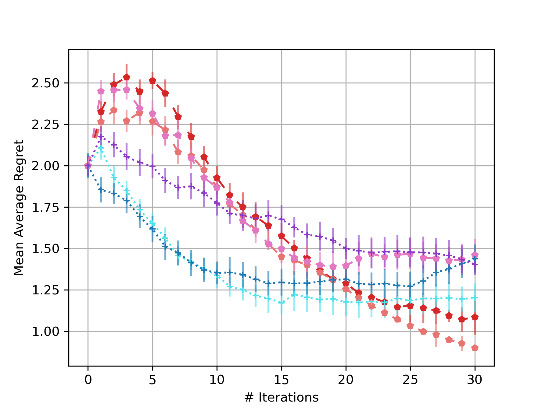
(a) Hartmann-3d

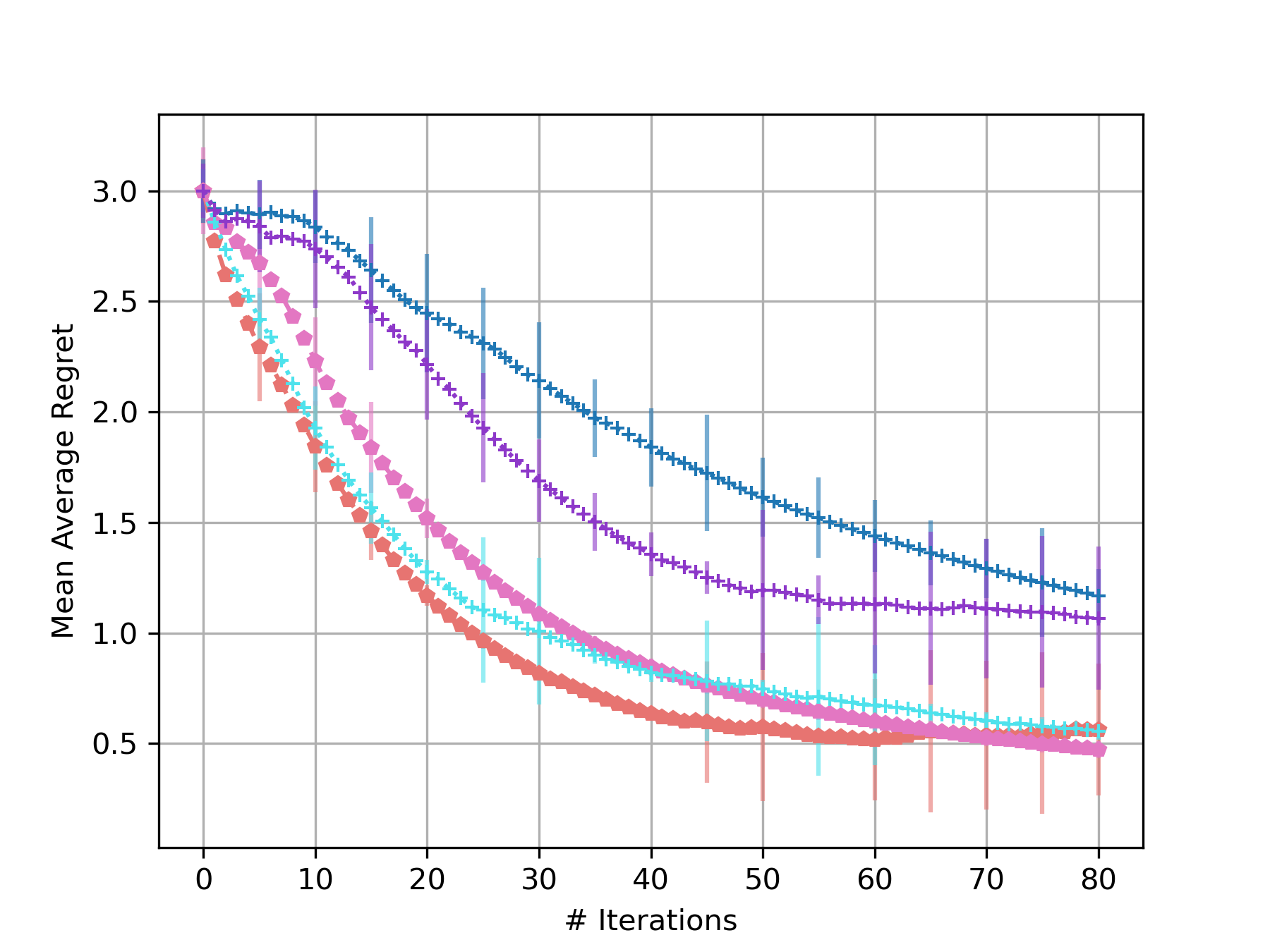
(b) Hartmann-6d

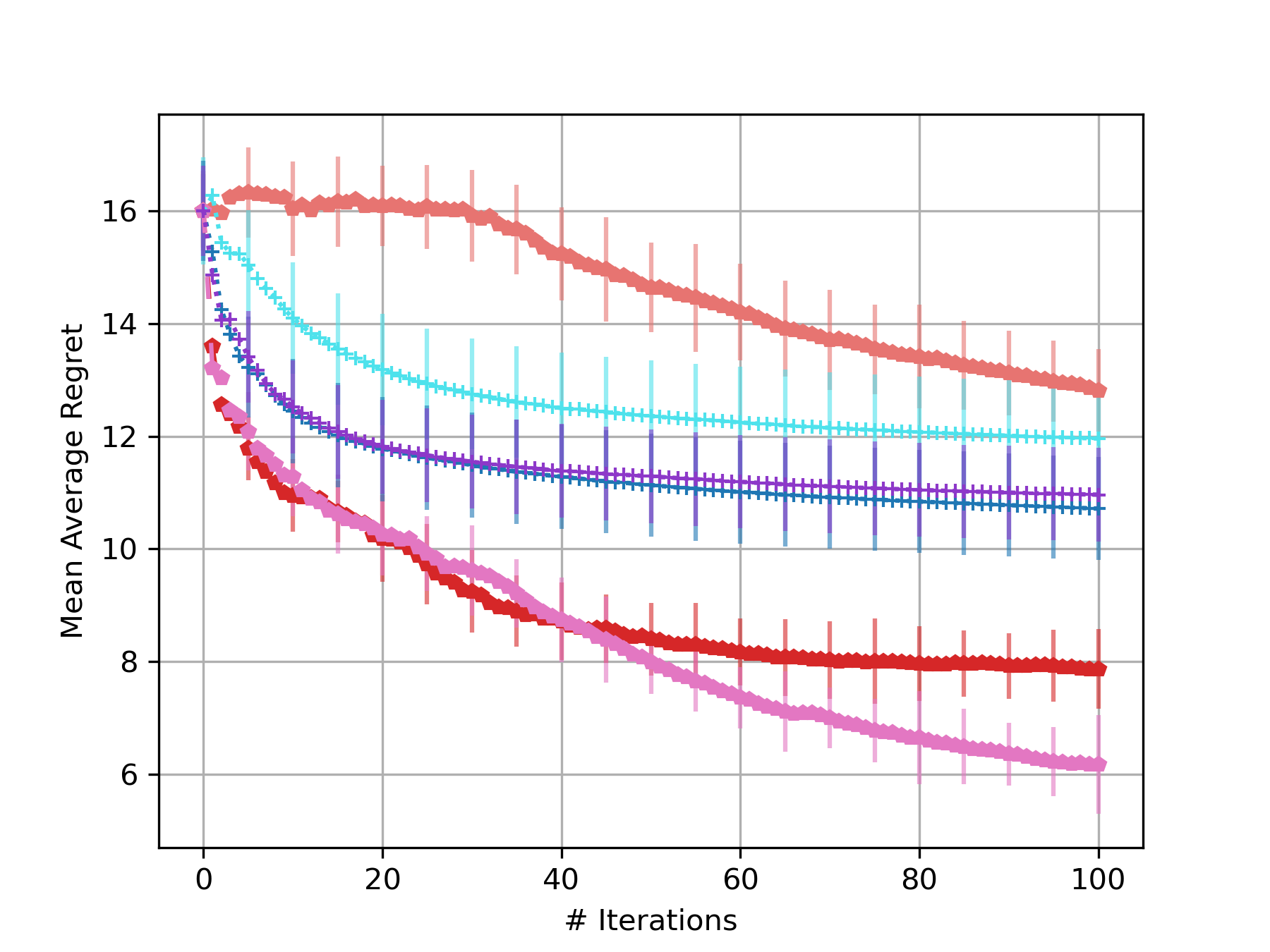
(c) Robot-3d

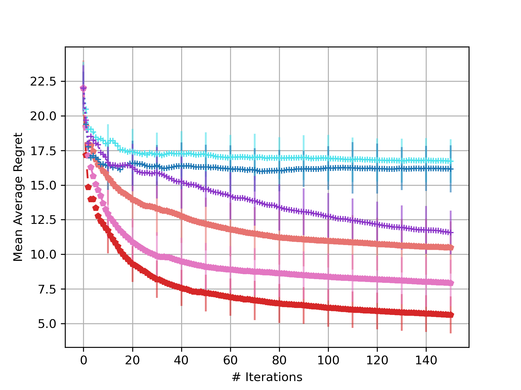
(D) Robot-4d

Figure 4: Results for the average mean regret over iterations using UCB as the acquisition function.

C.5 Alternative Acquisition Functions

To address potential bias from acquisition function selection, we repeated experiments using EI and PI alongside UCB. Results show that our approach outperformed baselines regardless of the choice acquisition function in nearly all cases, as shown in Figures 5 and 6.

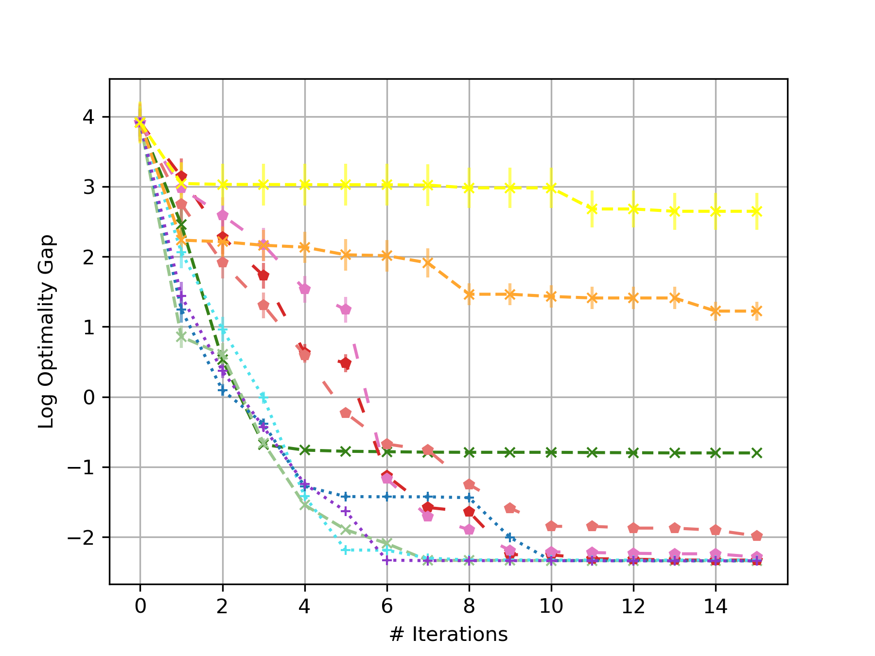
(a) Branin-2d

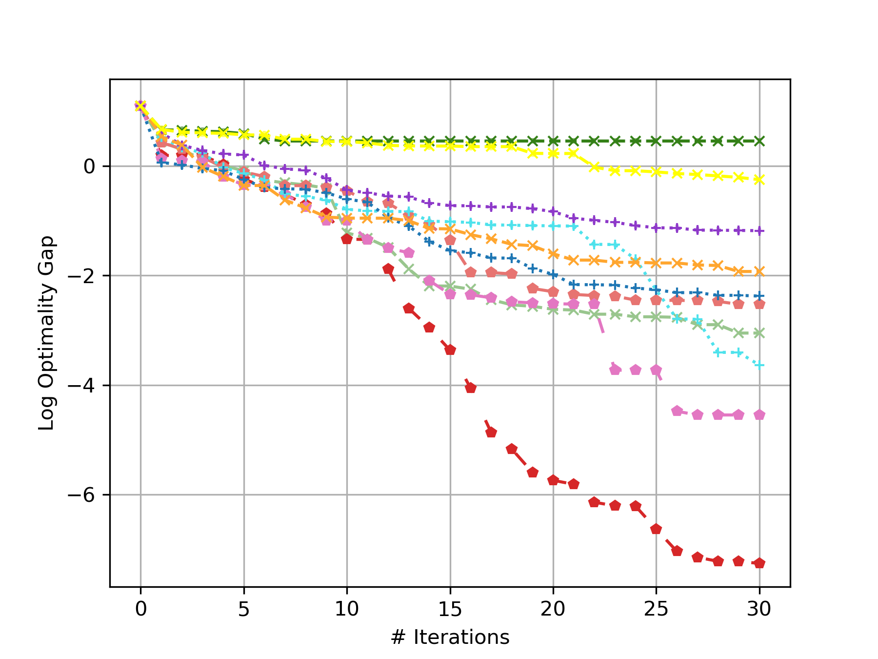
(b) Hartmann-3d

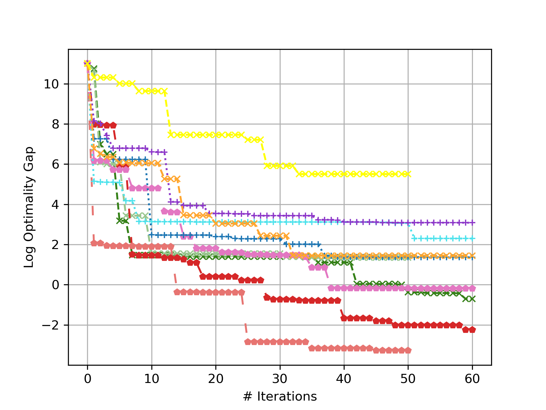
(c) Exponential-5d

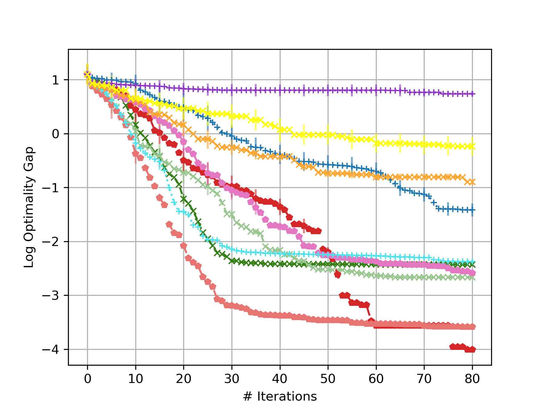
(d) Hartmann-6d

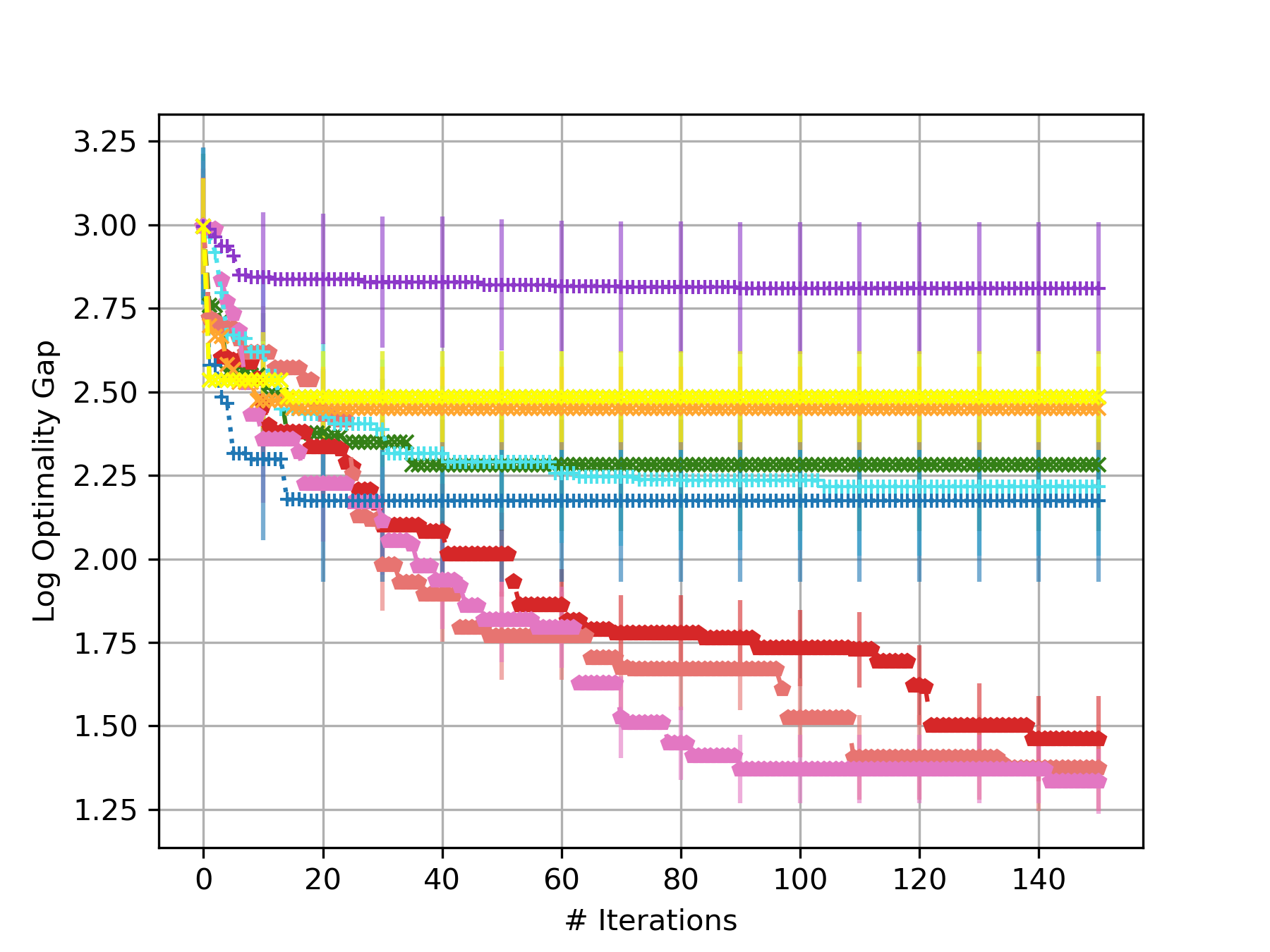
(e) Exponential-10d

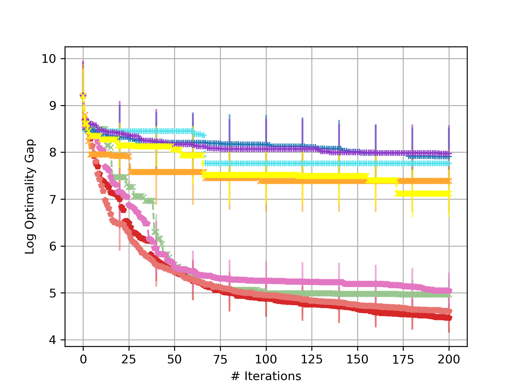
(f) Rosenbrock-20d

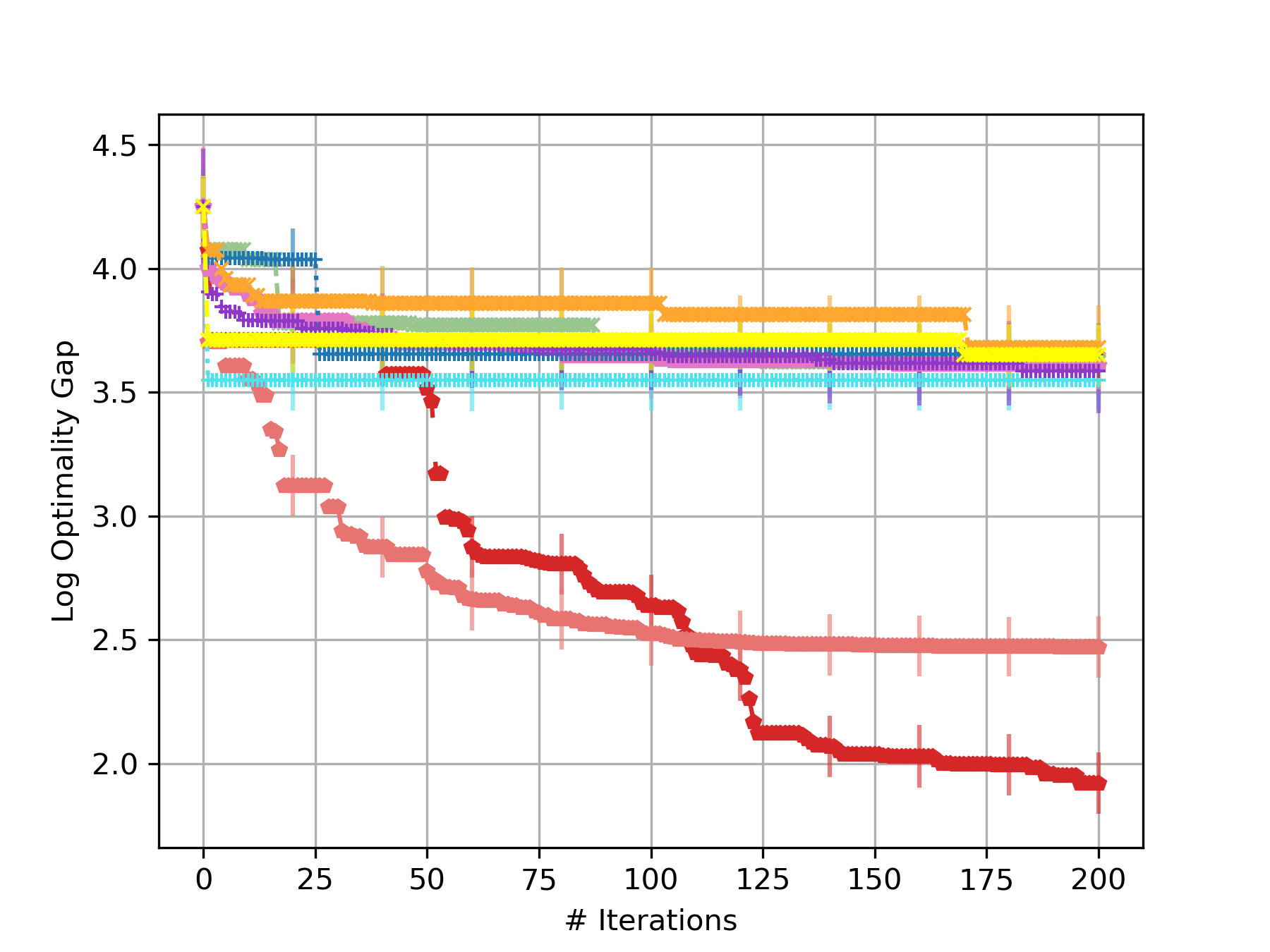
(g) Levy-30d

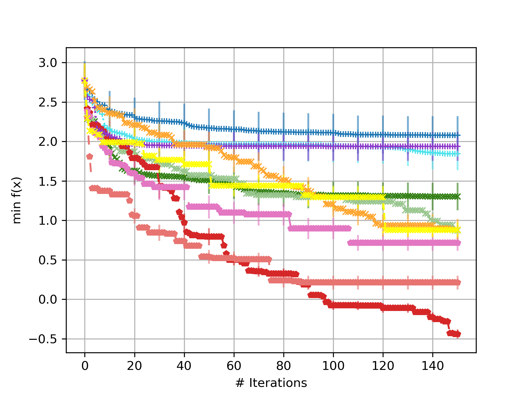
(h) Robot-4d

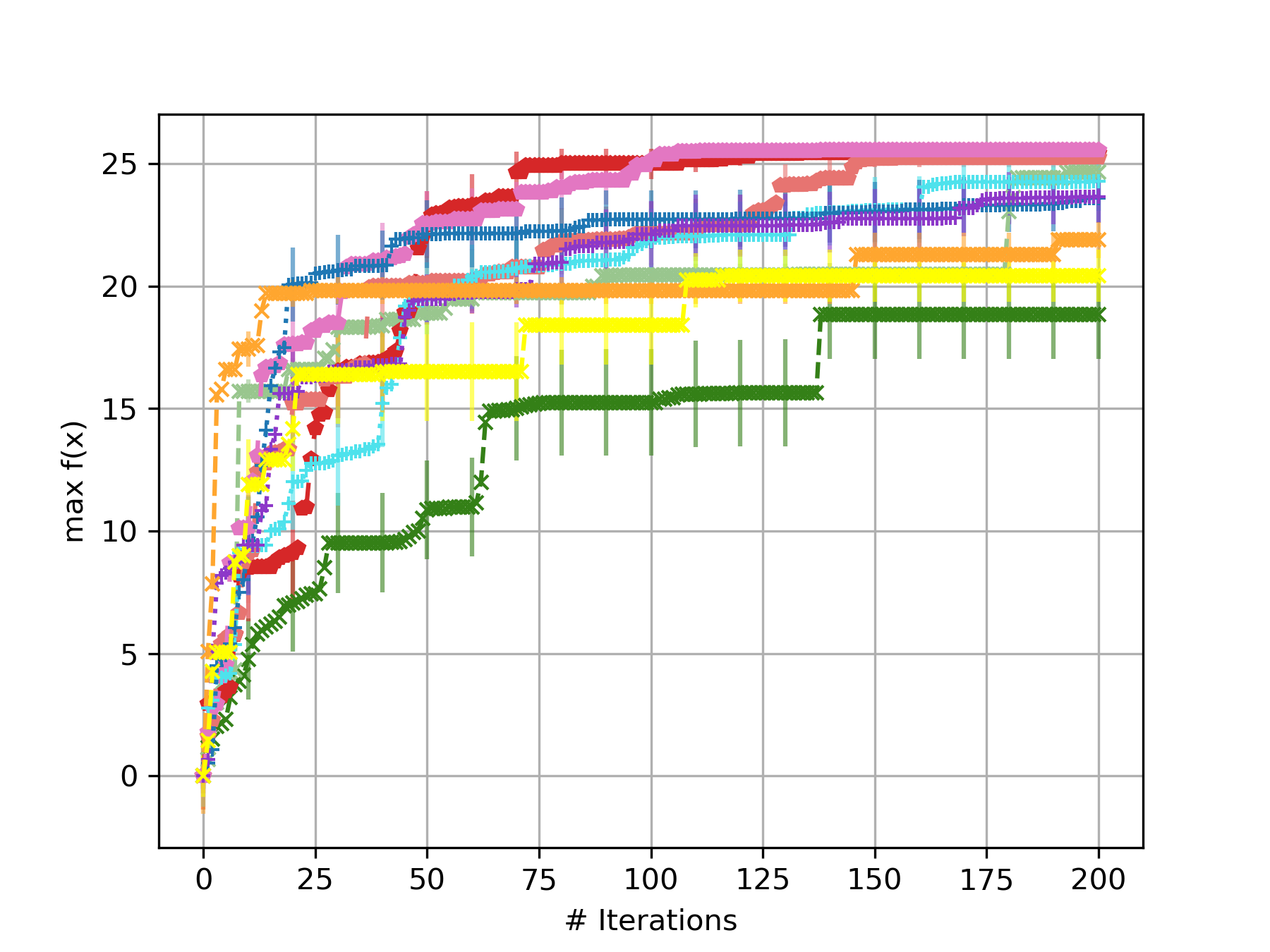
(i) Portfolio-5d

Figure 5: Optimization performance of different test functions and algorithms across 10 repetitions using EI acquisition function.

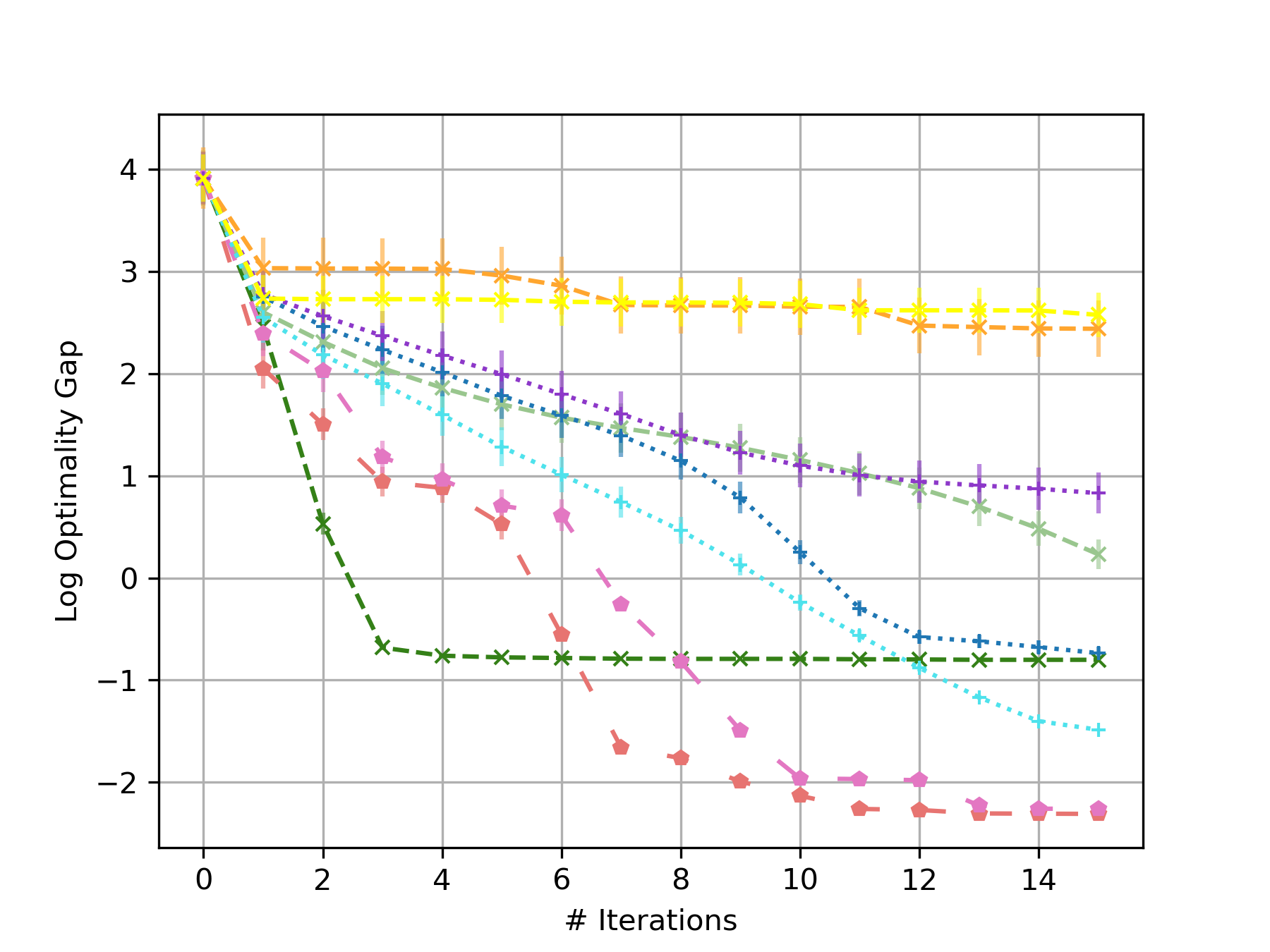
(a) Branin-2d

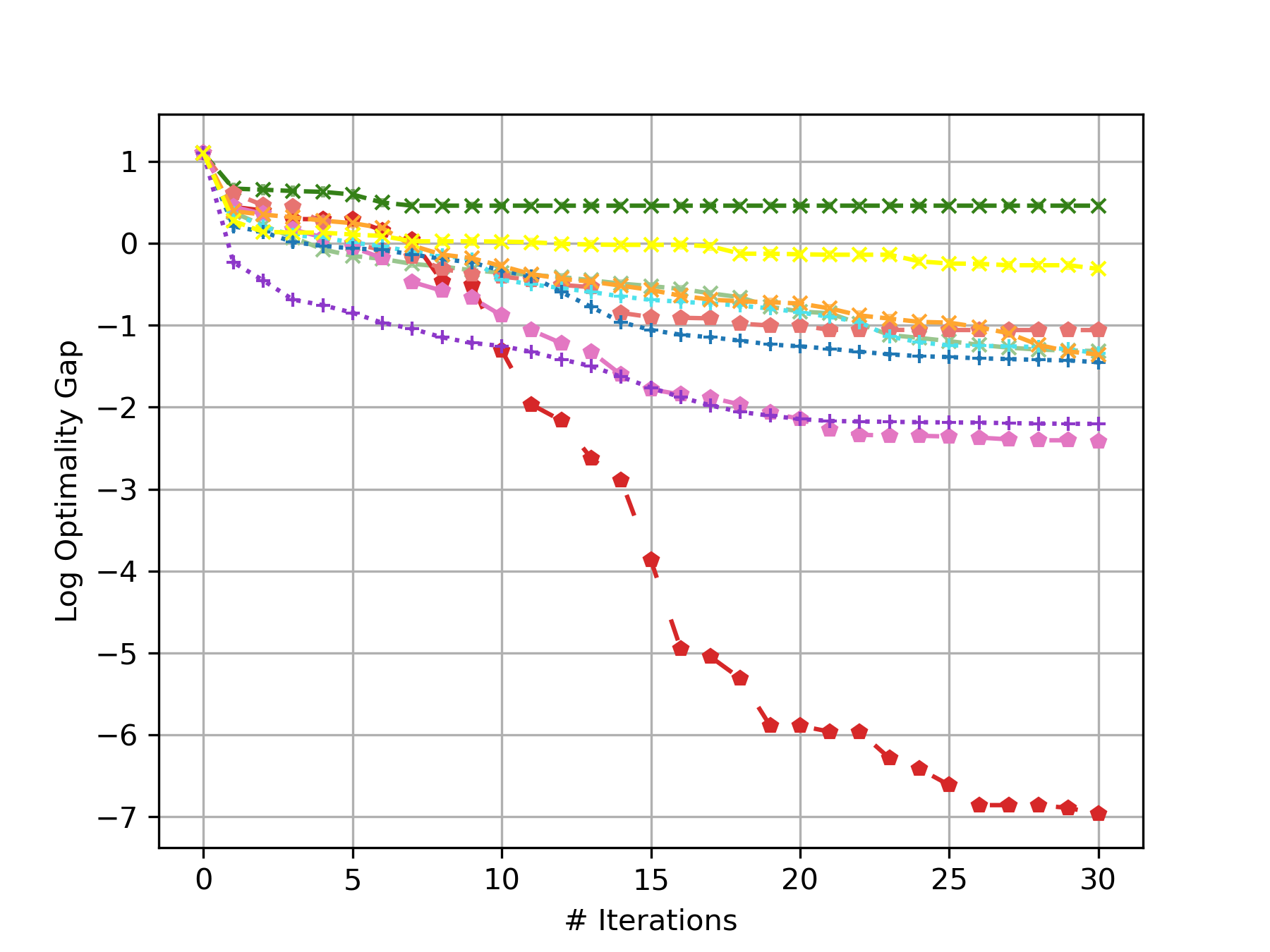
(b) Hartmann-3d

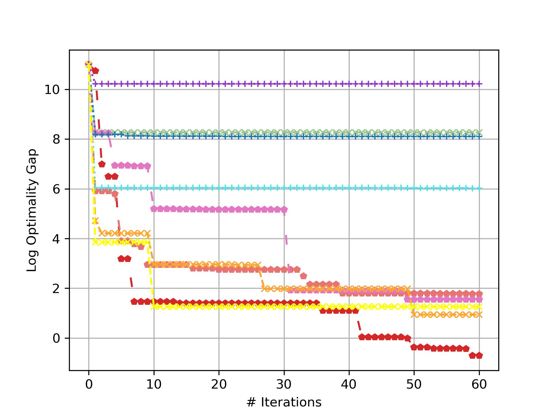
(c) Exponential-5d

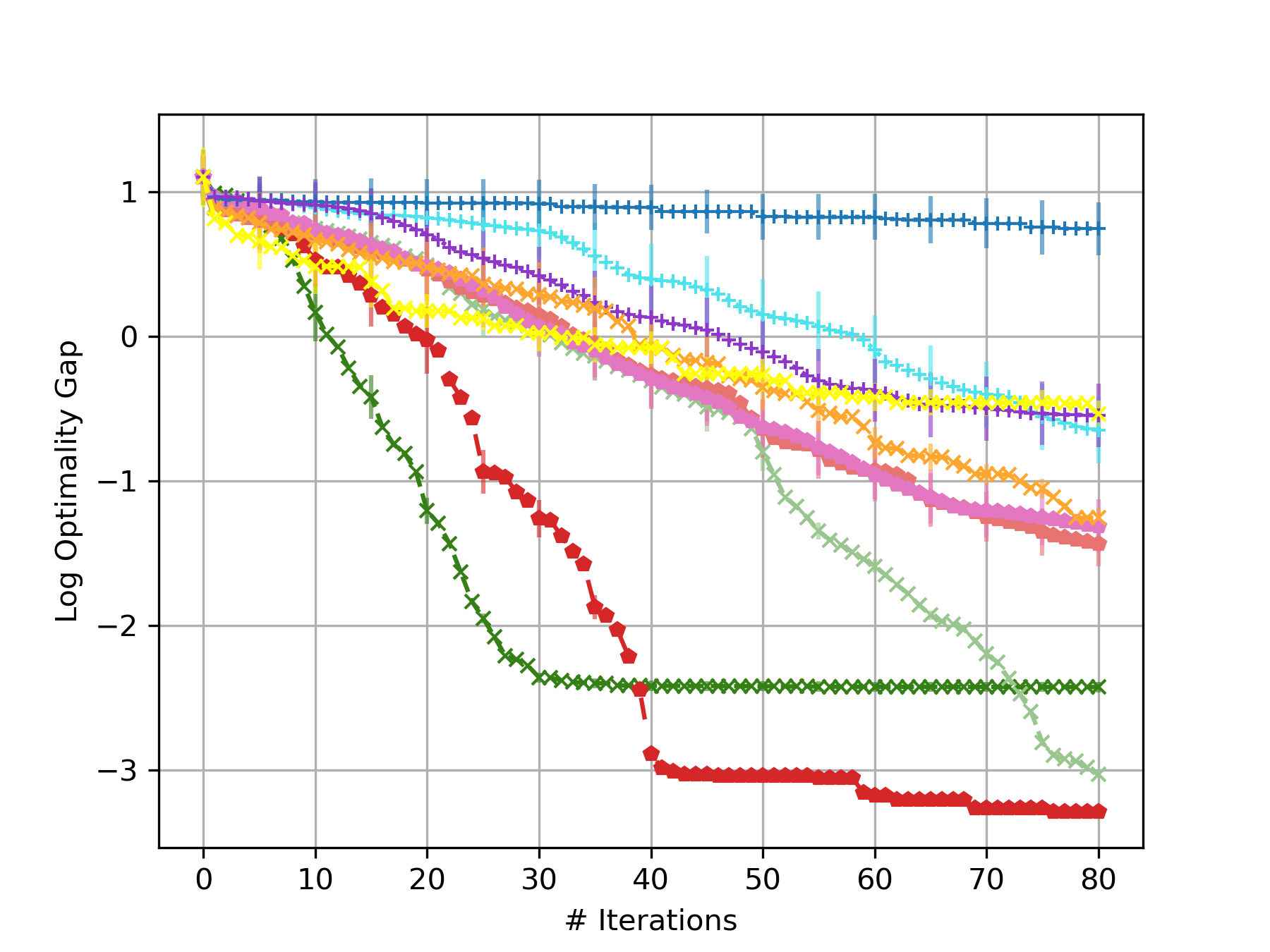
(d) Hartmann-6d

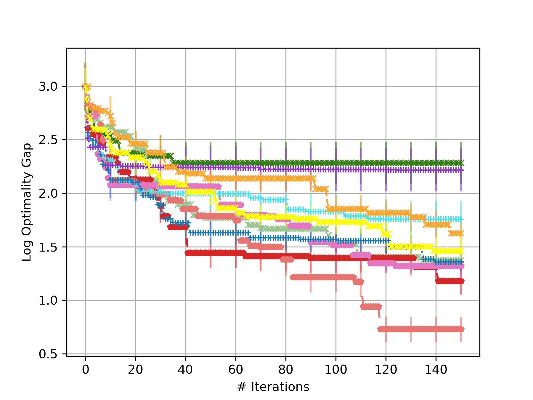
(e) Exponential-10d

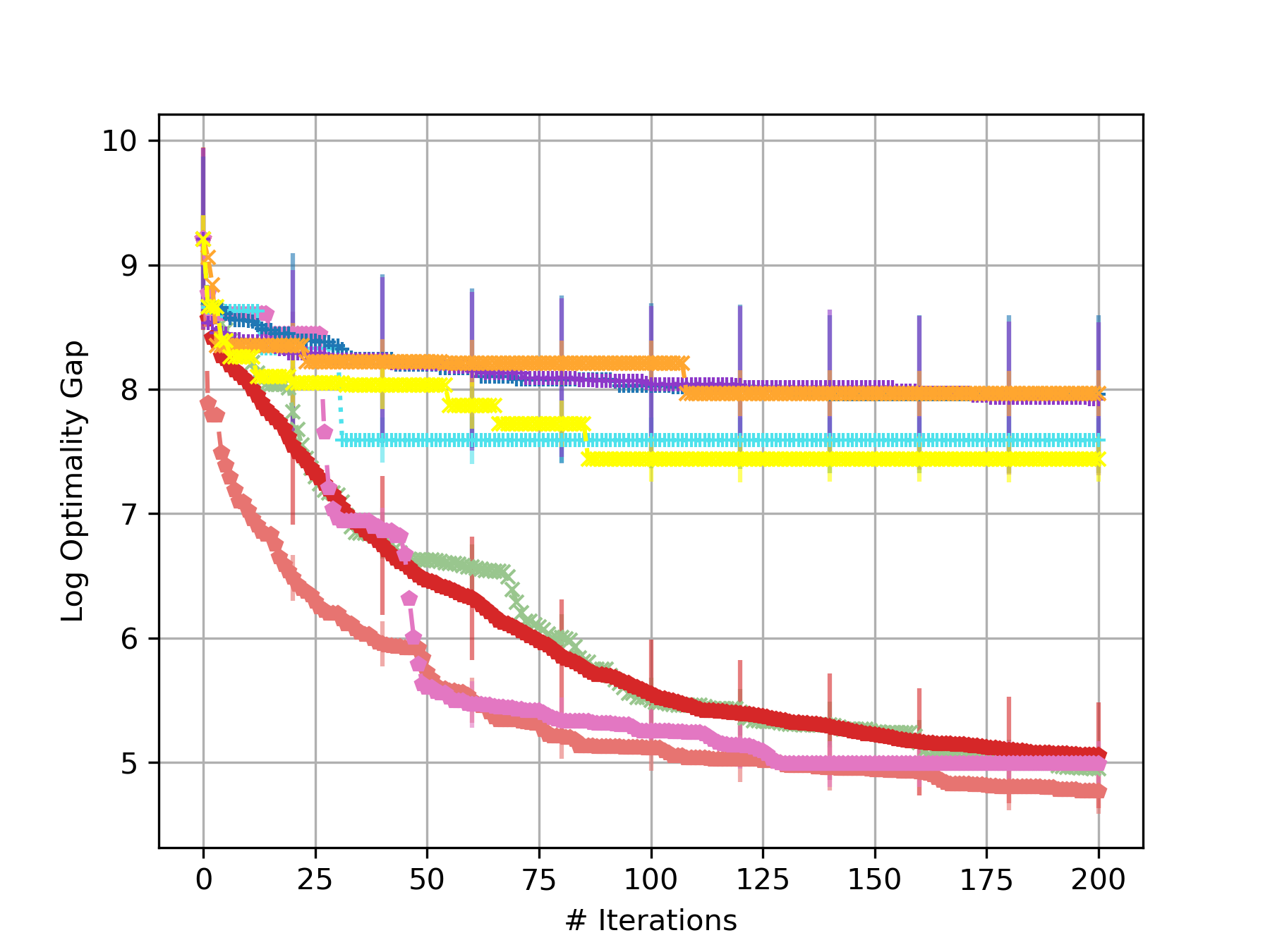
(f) Rosenbrock-20d

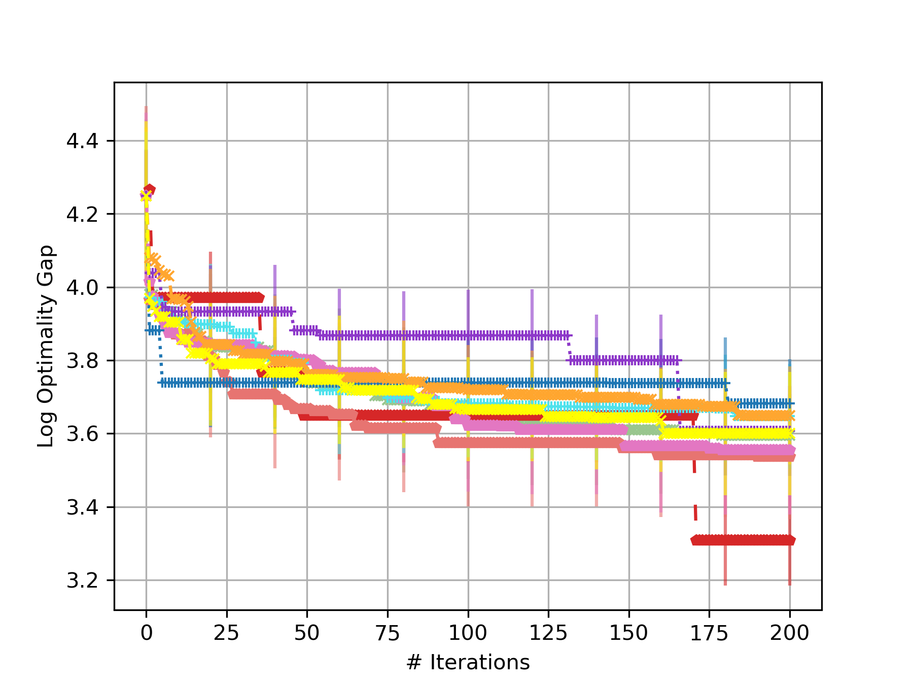
(g) Levy-30d

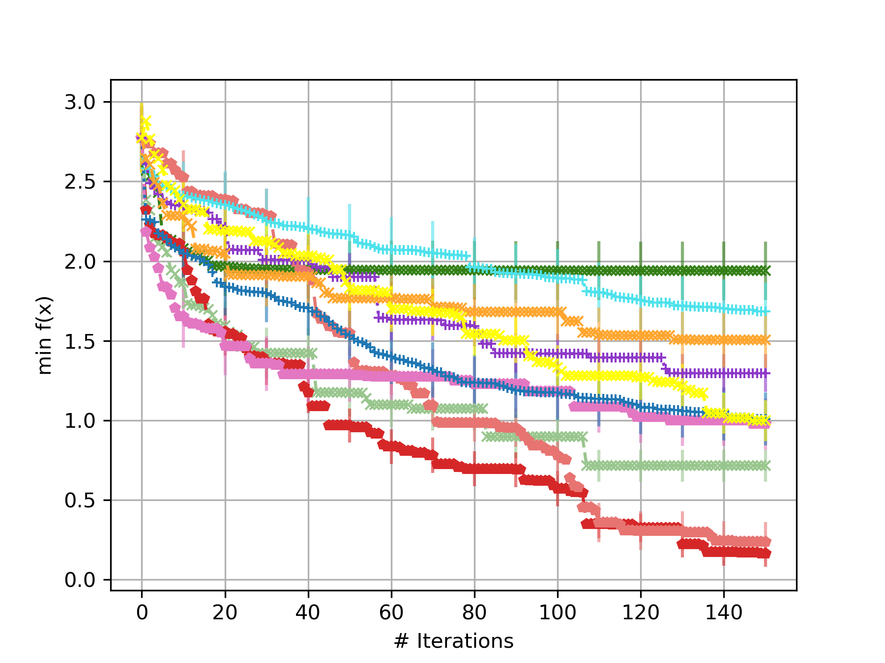
(h) Robot-4d

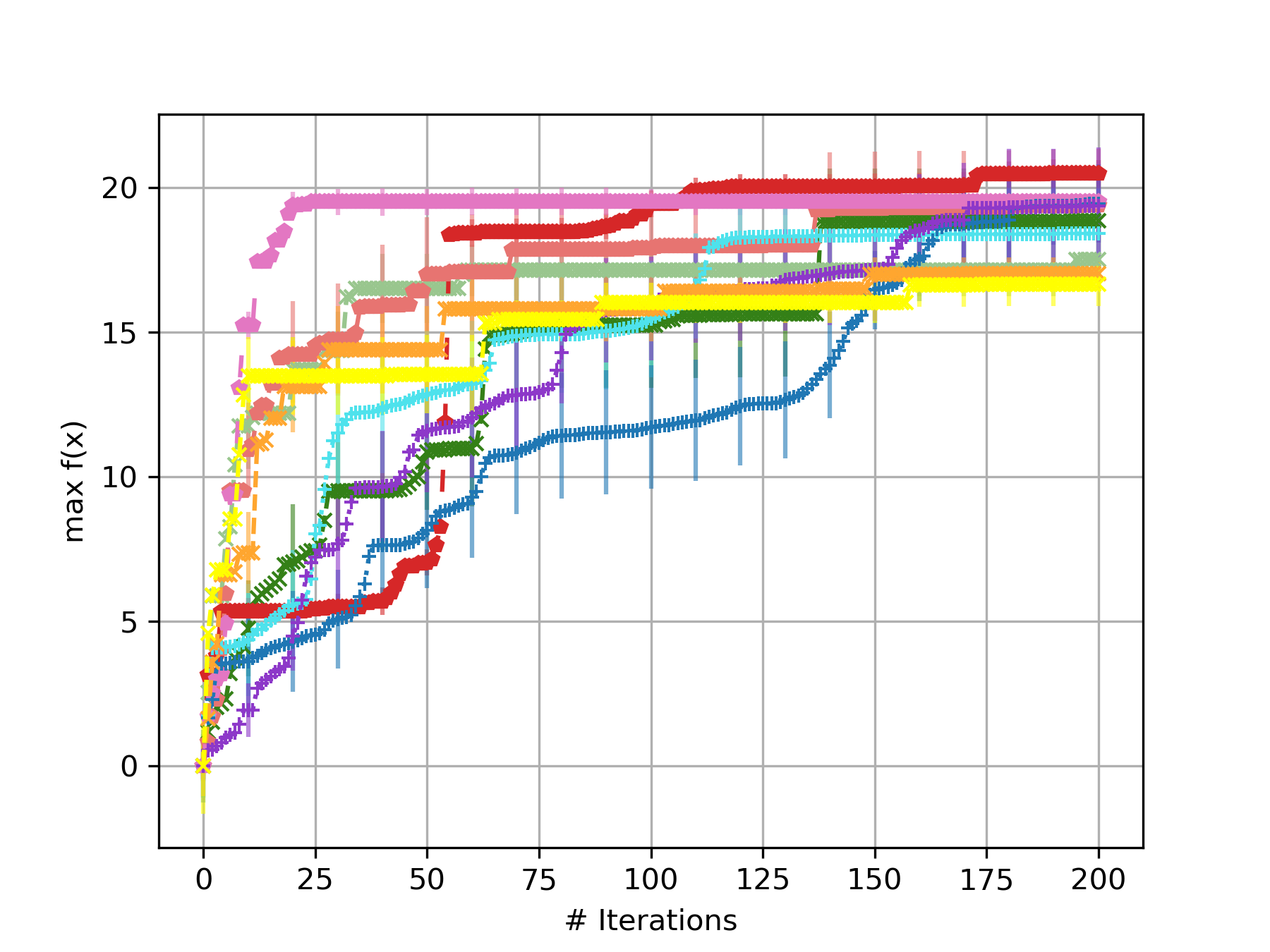
(i) Portfolio-5d

Figure 6: Optimization performance of different test functions and algorithms across 10 repetitions using PI acquisition function. Implementation constraint: original implementation of ABO exclusively uses EI; reported PI results for ABO are EI-based to enable cross-algorithm comparison.

C.6 Different Number of Spectral Mixtures

To illustrate the performance differences resulting from varying the number of mixture components, we further compare the performance of spectral mixture kernels combining Cauchy and Gaussian components, as illustrated in Figure 7. Across all tasks, there is a noticeable trend where specific configurations of Cauchy and Gaussian components yield superior optimization performance, as indicated by the larger bubbles. Additionally, the performance varies across tasks, highlighting the interplay between kernel structure and task-specific characteristics. The results emphasize the utility of balancing Cauchy and Gaussian components to achieve optimal performance in diverse optimization scenarios.

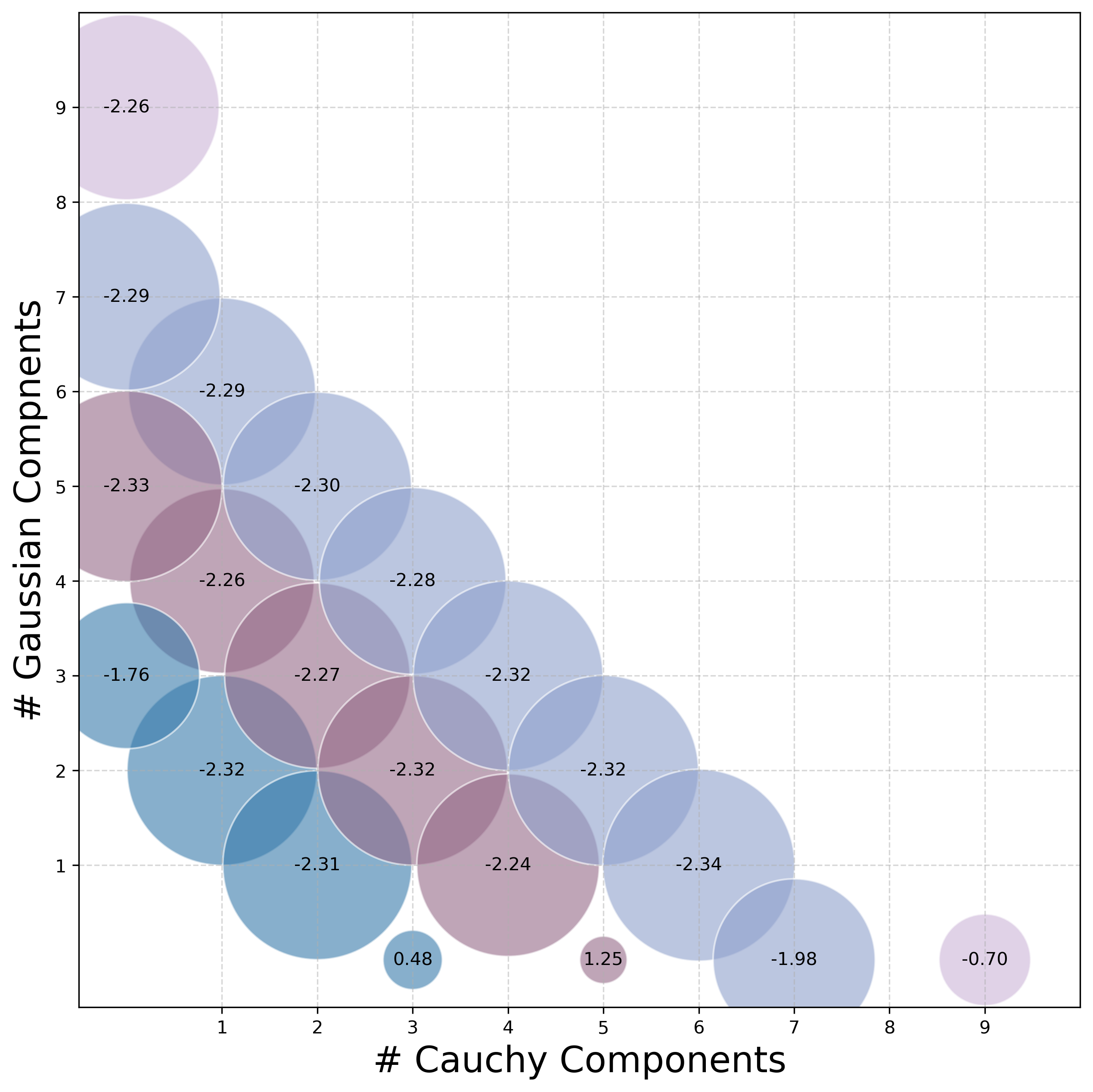
(a) Branin-2d

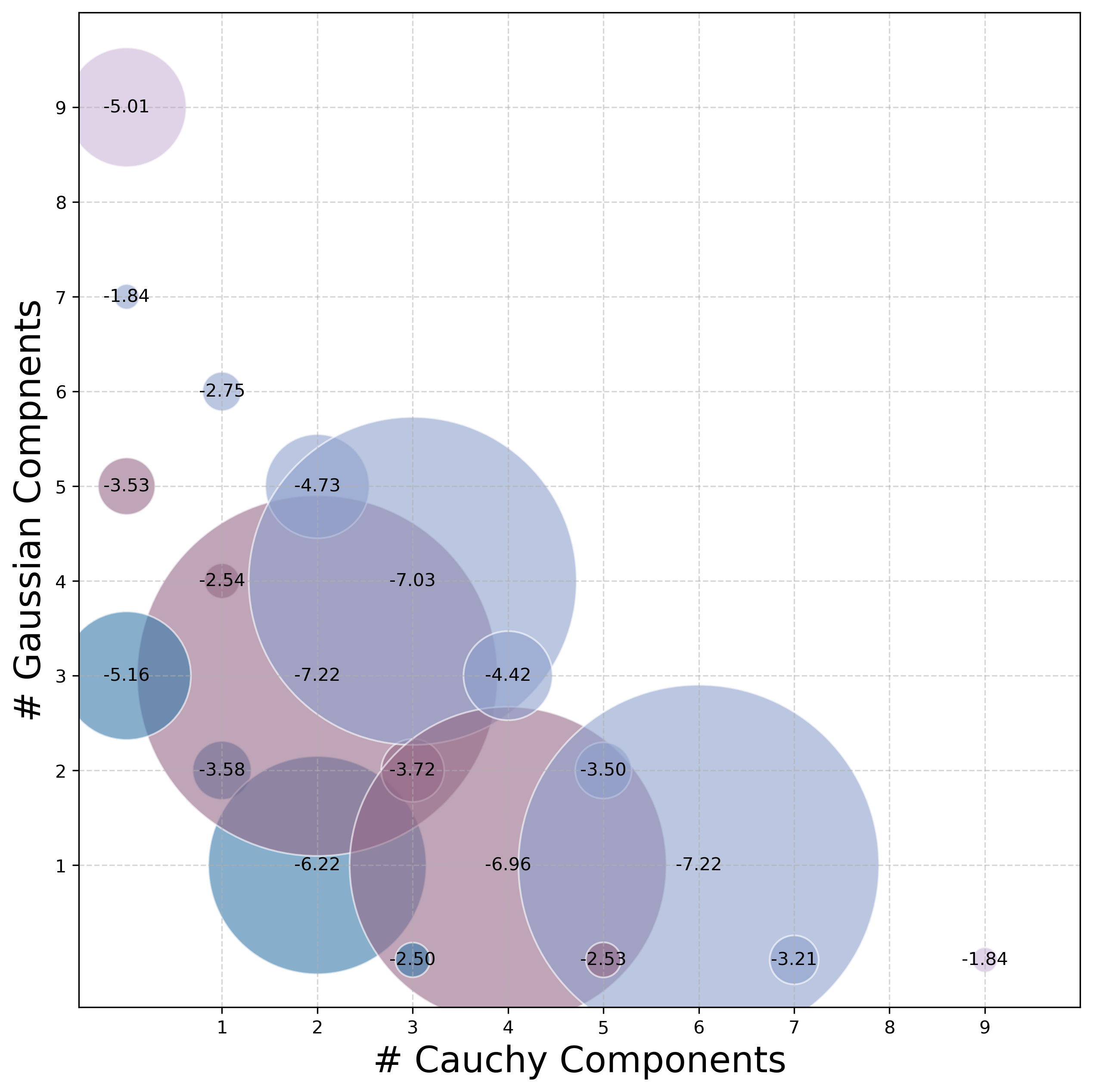
(b) Hartmann-3d

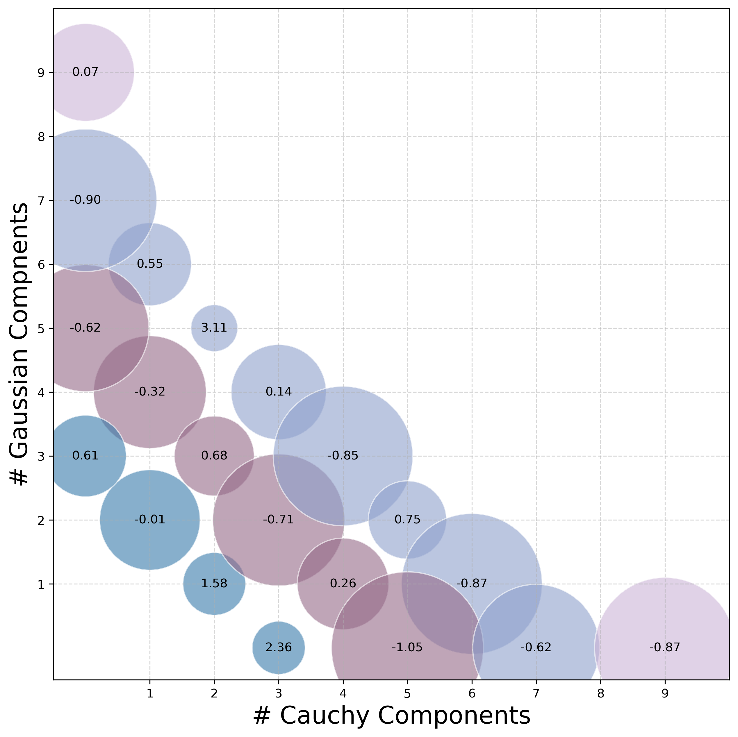
(c) Exponential-5d

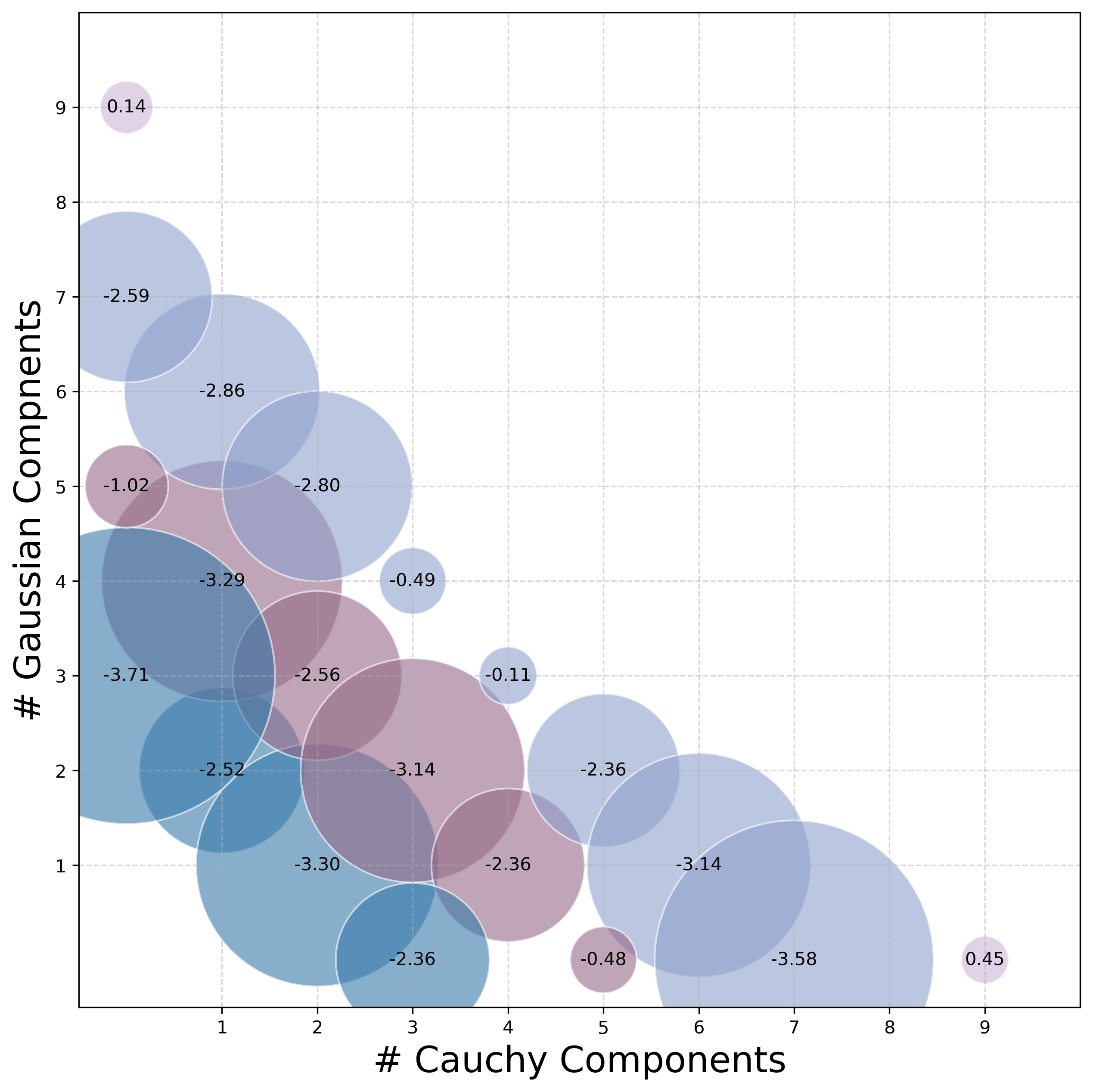
(d) Hartmann-6d

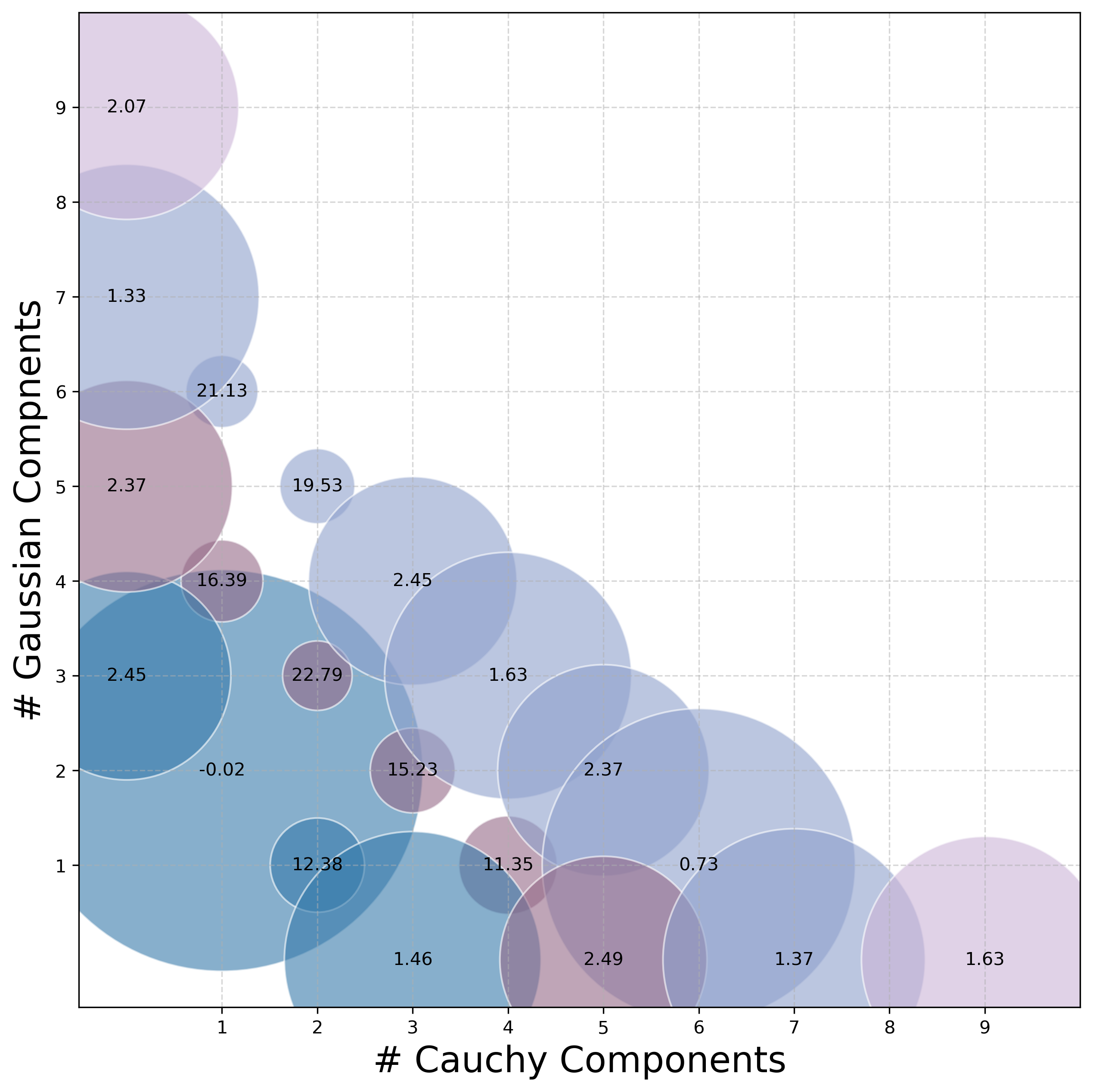
(e) Exponential-10d

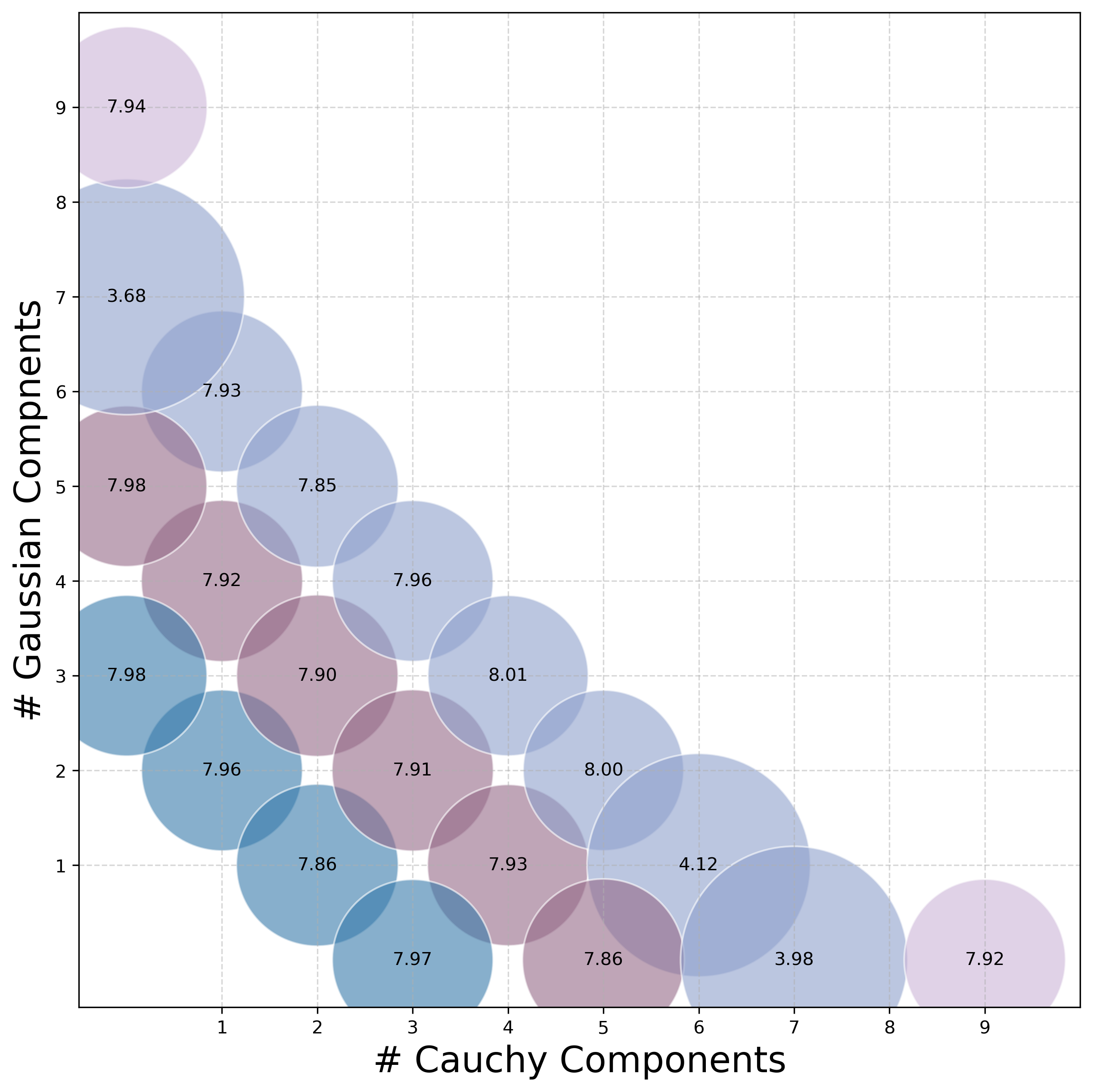
(f) Rosen-20d

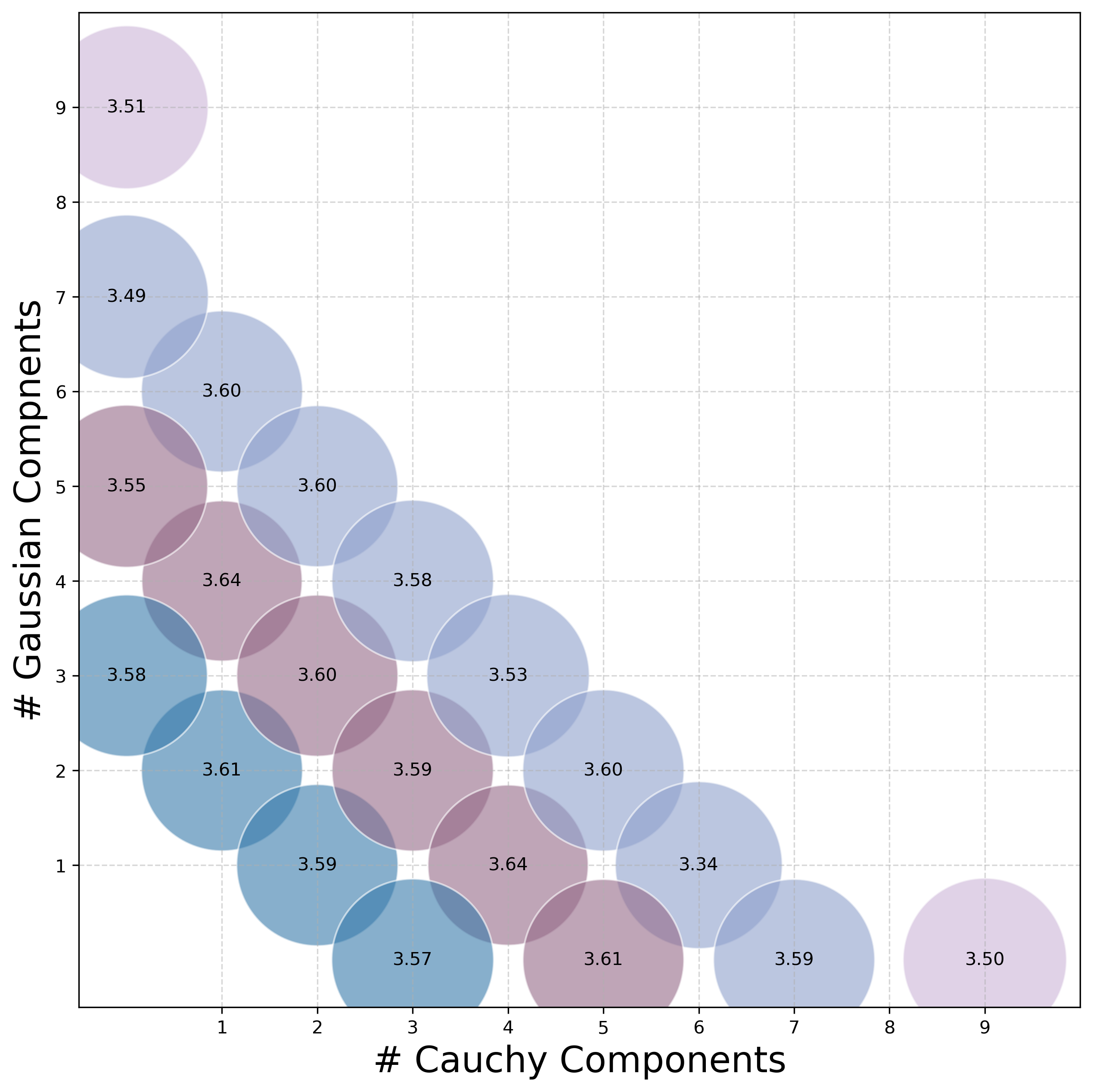
(g) Levy-30d

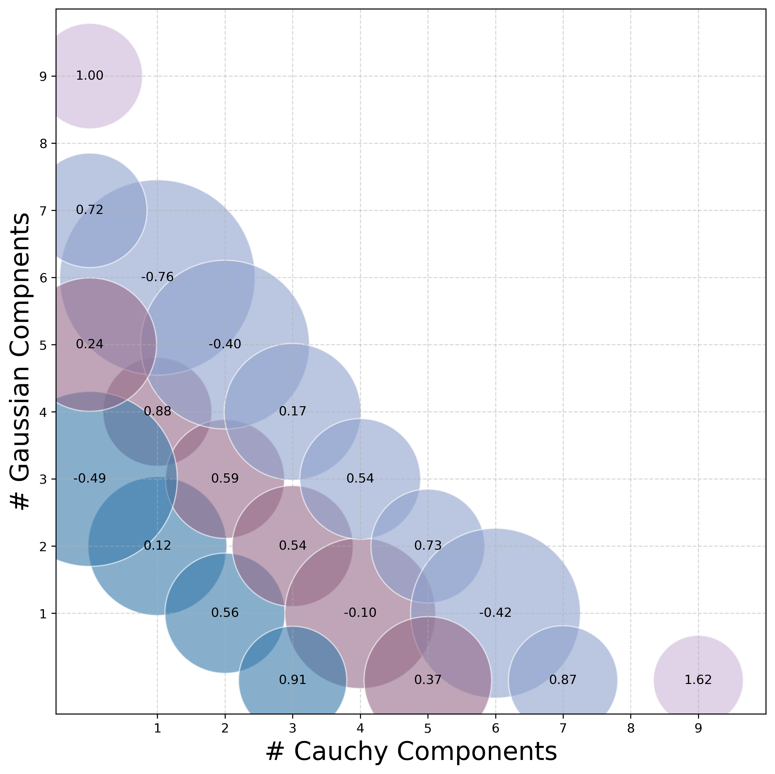
(h) Robot Pushing-4d

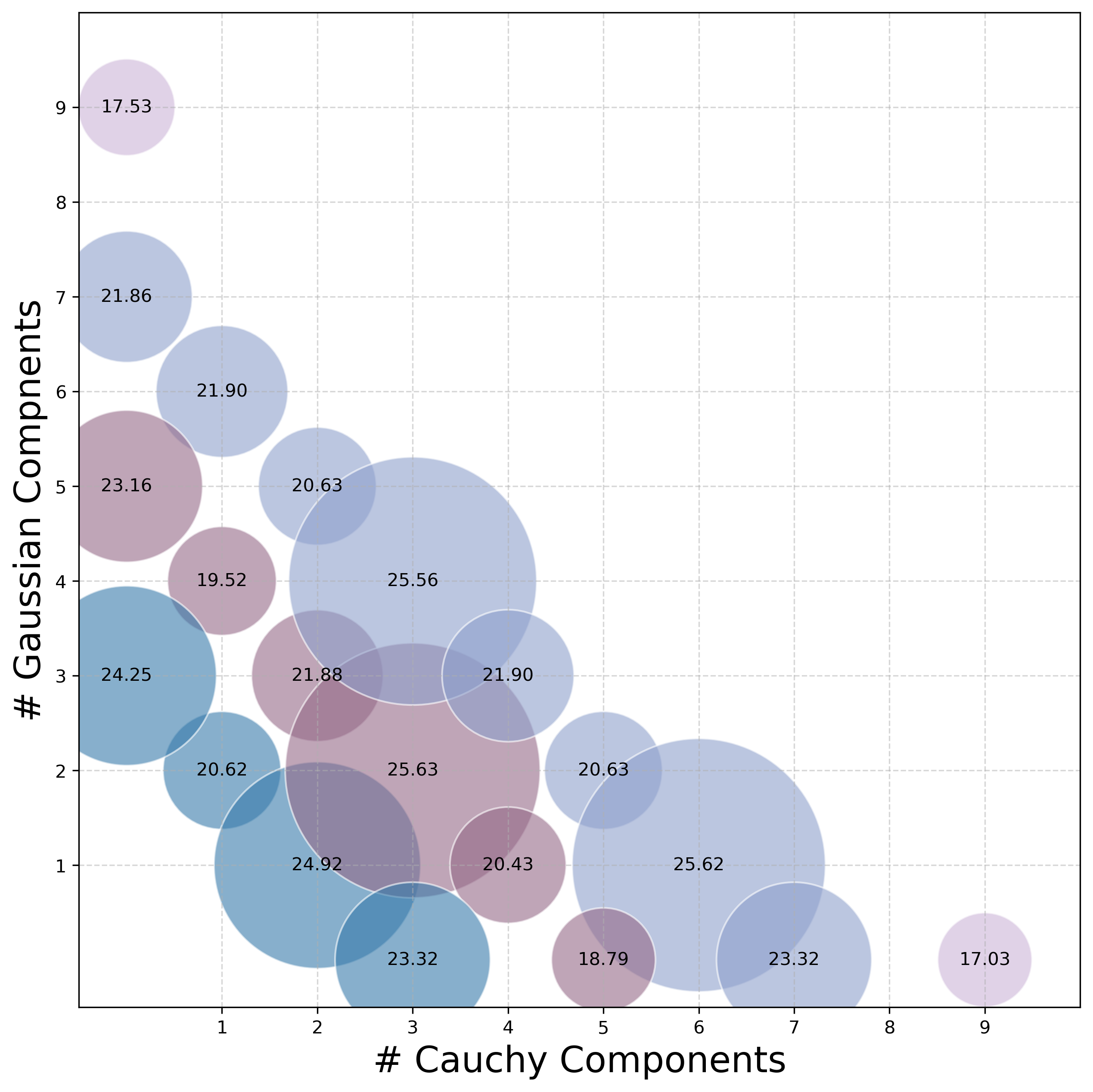
(i) portfolio-5d

Figure 7: Results for spectral mixture kernels with different number of Cauchy and Gaussian mixtures. The x-axis represents the number of Cauchy components, and the y-axis represents the number of Gaussian components. Different colors are used to distinguish mixtures based on their total number of components (3, 5, 7, 9). The bubble size represents the inverse of the optimality results, with larger bubbles indicating better performance.

References

- (1) Shipra Agrawal and Navin Goyal. Analysis of thompson sampling for the multi-armed bandit problem. In Shie Mannor, Nathan Srebro, and Robert C. Williamson, editors, Proceedings of the 25th Annual Conference on Learning Theory, volume 23 of Proceedings of Machine Learning Research, pages 39.1–39.26, Edinburgh, Scotland, 25–27 Jun 2012. PMLR.
- (2) Matias Altamirano and Felipe Tobar. Nonstationary multi-output gaussian processes via harmonizable spectral mixtures. In Gustau Camps-Valls, Francisco J. R. Ruiz, and Isabel Valera, editors, Proceedings of The 25th International Conference on Artificial Intelligence and Statistics, volume 151 of Proceedings of Machine Learning Research, pages 3204–3218. PMLR, 28–30 Mar 2022.
- (3) Stephen Boyd, Enzo Busseti, Steven Diamond, Ronald N. Kahn, Kwangmoo Koh, Peter Nystrup, and Jan Speth. 2017.
- (4) Sait Cakmak, Raul Astudillo, Peter Frazier, and Enlu Zhou. Bayesian optimization of risk measures. In Proceedings of the 34th International Conference on Neural Information Processing Systems, NIPS ’20, Red Hook, NY, USA, 2020. Curran Associates Inc.
- (5) Chris Chatfield. The Analysis of Time Series: An Introduction. CRC Press, 03 2016.
- (6) Peter I. Frazier, Warren B. Powell, and Savas Dayanik. A knowledge-gradient policy for sequential information collection. SIAM Journal on Control and Optimization, 47(5):2410–2439, 2008.
- (7) Peter I. Frazier and Jialei Wang. Bayesian Optimization for Materials Design, pages 45–75. Springer International Publishing, Cham, 2016.
- (8) Jacob Gardner, Chuan Guo, Kilian Weinberger, Roman Garnett, and Roger Grosse. Discovering and Exploiting Additive Structure for Bayesian Optimization. In Aarti Singh and Jerry Zhu, editors, Proceedings of the 20th International Conference on Artificial Intelligence and Statistics, volume 54 of Proceedings of Machine Learning Research, pages 1311–1319. PMLR, 20–22 Apr 2017.
- (9) Roman Garnett. Bayesian Optimization. Cambridge University Press, 2023.
- (10) Leslie Pack Kaelbling and Tomás Lozano-Pérez. Learning composable models of parameterized skills. In 2017 IEEE International Conference on Robotics and Automation (ICRA), pages 886–893, 2017.
- (11) Kirthevasan Kandasamy, Willie Neiswanger, Jeff Schneider, Barnabás Póczos, and Eric P. Xing. Neural architecture search with bayesian optimisation and optimal transport. In Proceedings of the 32nd International Conference on Neural Information Processing Systems, NIPS’18, page 2020–2029, Red Hook, NY, USA, 2018. Curran Associates Inc.
- (12) Kirthevasan Kandasamy, Jeff Schneider, and Barnabás Póczos. High dimensional bayesian optimisation and bandits via additive models. In Proceedings of the 32nd International Conference on International Conference on Machine Learning - Volume 37, ICML’15, page 295–304. JMLR.org, 2015.
- (13) Hermann König. Eigenvalue Distribution of Compact Operators. Springer Basel AG, 1986.
- (14) Miguel Lázaro-Gredilla, Joaquin Quiñonero Candela, Carl Edward Rasmussen, and Aníbal R. Figueiras-Vidal. Sparse spectrum gaussian process regression. J. Mach. Learn. Res., 11:1865–1881, August 2010.
- (15) Romy Lorenz, Laura E. Simmons, Ricardo P. Monti, Joy L. Arthur, Severin Limal, Ilkka Laakso, Robert Leech, and Ines R. Violante. Efficiently searching through large tacs parameter spaces using closed-loop bayesian optimization. Brain Stimulation, 12(6):1484–1489, 2019.
- (16) Gustavo Malkomes and Roman Garnett. Automating bayesian optimization with bayesian optimization. In Proceedings of the 32th International Conference on Neural Information Processing Systems, NIPS’18, page 5988–5997, Red Hook, NY, USA, 2018. Curran Associates Inc.
- (17) J. Mockus. On the bayes methods for seeking the extremal point. IFAC Proceedings Volumes, 8(1, Part 1):428–431, 1975. 6th IFAC World Congress (IFAC 1975) - Part 1: Theory, Boston/Cambridge, MA, USA, August 24-30, 1975.
- (18) Quoc Phong Nguyen, Zhongxiang Dai, Bryan Kian Hsiang Low, and Patrick Jaillet. Value-at-risk optimization with gaussian processes. In Marina Meila and Tong Zhang, editors, Proceedings of the 38th International Conference on Machine Learning, volume 139 of Proceedings of Machine Learning Research, pages 8063–8072. PMLR, 18–24 Jul 2021.
- (19) Art B. Owen. Scrambling sobol’ and niederreiter–xing points. Journal of Complexity, 14(4):466–489, 1998.
- (20) Gabriel Parra and Felipe Tobar. Spectral mixture kernels for multi-output gaussian processes. In I. Guyon, U. Von Luxburg, S. Bengio, H. Wallach, R. Fergus, S. Vishwanathan, and R. Garnett, editors, Advances in Neural Information Processing Systems, volume 30. Curran Associates, Inc., 2017.
- (21) Konstantinos Plataniotis and D. Hatzinakos. Gaussian mixtures and their applications to signal processing, page 36. CRC Press, 01 2000.
- (22) Carl Edward Rasmussen and Christopher K. I. Williams. Gaussian Processes for Machine Learning. The MIT Press, 11 2006.
- (23) Ibai Roman, Roberto Santana, Alexander Mendiburu, and Jose A. Lozano. An experimental study in adaptive kernel selection for bayesian optimization. IEEE Access, 7:184294–184302, 2019.
- (24) Yves-Laurent Kom Samo and Stephen Roberts. Generalized spectral kernels, 2015.
- (25) Matthias W. Seeger, Sham M. Kakade, and Dean P. Foster. Information consistency of nonparametric gaussian process methods. IEEE Transactions on Information Theory, 54(5):2376–2382, 2008.
- (26) Fergus Simpson, Alexis Boukouvalas, Vaclav Cadek, Elvijs Sarkans, and Nicolas Durrande. The minecraft kernel: Modelling correlated gaussian processes in the fourier domain. In Arindam Banerjee and Kenji Fukumizu, editors, Proceedings of The 24th International Conference on Artificial Intelligence and Statistics, volume 130 of Proceedings of Machine Learning Research, pages 1945–1953. PMLR, 13–15 Apr 2021.
- (27) Niranjan Srinivas, Andreas Krause, Sham M. Kakade, and Matthias W. Seeger. Information-theoretic regret bounds for gaussian process optimization in the bandit setting. IEEE Transactions on Information Theory, 58(5):3250–3265, 2012.
- (28) Michael L. Stein. Interpolation of Spatial Data: Some Theory for Kriging. Springer New York, 1999.
- (29) S. Surjanovic and D. Bingham. Virtual library of simulation experiments: Test functions and datasets. Retrieved January 19, 2025, from http://www.sfu.ca/˜ssurjano, 2025.
- (30) Felipe Tobar. Band-limited gaussian processes: the sinc kernel. Curran Associates Inc., Red Hook, NY, USA, 2019.
- (31) Salomon Trust. Lectures on Fourier Integrals. Princeton University Press, Princeton, 1960.
- (32) Matteo Turchetta, Andreas Krause, and Sebastian Trimpe. Robust model-free reinforcement learning with multi-objective bayesian optimization. In 2020 IEEE International Conference on Robotics and Automation (ICRA), pages 10702–10708, 2020.
- (33) Rodrigo Vargas-Hernández and Jake Gardner. Gaussian processes with spectral delta kernel for higher accurate potential energy surfaces for large molecules, 09 2021.
- (34) Zi Wang and Stefanie Jegelka. Max-value entropy search for efficient bayesian optimization. In Proceedings of the 34th International Conference on Machine Learning - Volume 70, ICML’17, page 3627–3635. JMLR.org, 2017.
- (35) Harold Widom. Asymptotic behavior of the eigenvalues of certain integral equations. Transactions of the American Mathematical Society, 109:278–295, 1963.
- (36) Andrew Gordon Wilson and Ryan Prescott Adams. Gaussian process kernels for pattern discovery and extrapolation. In Proceedings of the 30th International Conference on International Conference on Machine Learning - Volume 28, ICML’13, page III–1067–III–1075. JMLR.org, 2013.
- (37) Andrew Gordon Wilson, Elad Gilboa, Arye Nehorai, and John P. Cunningham. Fast kernel learning for multidimensional pattern extrapolation. In Proceedings of the 28th International Conference on Neural Information Processing Systems - Volume 2, NIPS’14, page 3626–3634, Cambridge, MA, USA, 2014. MIT Press.
- (38) Jian Wu, Saul Toscano-Palmerin, Peter I. Frazier, and Andrew Gordon Wilson. Practical multi-fidelity bayesian optimization for hyperparameter tuning. In Ryan P. Adams and Vibhav Gogate, editors, Proceedings of The 35th Uncertainty in Artificial Intelligence Conference, volume 115 of Proceedings of Machine Learning Research, pages 788–798. PMLR, 22–25 Jul 2020.
- (39) Ciyou Zhu, Richard H. Byrd, Peihuang Lu, and Jorge Nocedal. Algorithm 778: L-bfgs-b: Fortran subroutines for large-scale bound-constrained optimization. ACM Trans. Math. Softw., 23(4):550–560, December 1997.
- (40) Huaiyu Zhu, Christopher K. I. Williams, Richard Rohwer, and Michal Morciniec. Gaussian regression and optimal finite dimensional linear models. Technical report, Birmingham, July 1997.