Value-Guided Search for
Efficient Chain-of-Thought Reasoning

Abstract

In this paper, we propose a simple and efficient method for value model training on long-context reasoning traces. Compared to existing process reward models (PRMs), our method does not require a fine-grained notion of “step,” which is difficult to define for long-context reasoning models. By collecting a dataset of 2.5 million reasoning traces, we train a 1.5B token-level value model and apply it to DeepSeek models for improved performance with test-time compute scaling. We find that block-wise value-guided search (VGS) with a final weighted majority vote achieves better test-time scaling than standard methods such as majority voting or best-of-$n$. With an inference budget of 64 generations, VGS with DeepSeek-R1-Distill-1.5B achieves an average accuracy of $45.7\%$ across four competition math benchmarks (AIME 2024 & 2025, HMMT Feb 2024 & 2025), reaching parity with o3-mini-medium. Moreover, VGS significantly reduces the inference FLOPs required to achieve the same performance of majority voting. Our dataset, model and codebase are open-sourced at https://github.com/kaiwenw/value-guided-search.

Figure 1: Performance and Efficiency of Value Guidance: (Left) Value-guided search improves the overall quality of DeepSeek-R1-Distill responses across four combined competition math benchmarks (AIME & HMMT). The inference budget for 1.5B, 7B and 14B are $256$, $128$ and $64$ generations, respectively. (Right) Value-guided search also reduces the inference FLOPs required to achieve the same accuracy levels as majority voting, a standard TTC scaling baseline, showing value-guidance is promising for improving efficiency.

1 Introduction

Recent large language models (LLMs), such as OpenAI o1 & o3, Claude Sonnet 3.7, Gemini Pro 2.5 and DeepSeek R1 [18] are trained via reinforcement learning (RL) to “think” for many tokens before generating a final answer. Through multi-step reasoning and self-correction, these reasoning models have state-of-the-art performance in competition math, coding [16] and scientific research [37], often surpassing the average human. However, this enhanced capability comes at a cost: each generation involves a long chain-of-thought (CoT), thus requiring more inference compute. Further, these CoT traces can often be repetitive and get stuck in unproductive loops [30]. This raises two questions. Can we extract the same performance at a fraction of the inference compute by refining the thinking process? Can we improve the performance ceiling of these models with productive search methods?

Search with guidance models is a natural solution that addresses longer chain-of-thought reasoning by managing the exponential growth of possible paths with guidance models identifying optimal routes [15, 39, 35]. Prior works that combined search with LLMs proposed to guide search with process reward models (PRMs), predicting the correctness of each step (e.g., delimited by newlines) in the model-generated solution [23, 44, 50]. While PRM-guided search has been shown to improve test-time compute (TTC) [6, 36, 34, 25], it is challenging to scale existing PRM training techniques to long-context reasoning models. First, existing methods require a pre-defined notion of “step,” but, per Guo et al. [18], “it is challenging to explicitly define a fine-grain step in general reasoning.” Second, even if we can define a “step,” collecting step-wise labels is prohibitively expensive, since it requires annotations from humans [23], LLM-as-a-Judge [50], or multiple Monte Carlo roll-outs [44, 27]. Thus, there has been limited success to scale PRMs to long-context reasoning models [18].

We propose value-guided search (VGS) – a block-level search method guided by a token-level value model – as a promising approach to scale TTC for reasoning models. In Section˜2, we present an effective pipeline for value model training on tasks with outcome labels, such as competition math. Our data pipeline collects solution prefixes from various models and then, starting from random prefixes, generates completed solutions using a lean reasoning model (e.g., DeepSeek-R1-Distill-1.5B). Notably, our data collection does not require a pre-defined notion of step and is more efficient than existing techniques [44, 27]. With this pipeline, we collect a dataset of 2.5 million math reasoning traces (over $30$ billion tokens) from a filtered subset of the OpenR1-Math dataset [2]. Then, we train a 1.5B token-level value model called DeepSeek-VM-1.5B by regressing (via classification) the final reward of the completed solution.

Next, in Section˜3, we apply our value model to perform block-wise search with DeepSeek models [18] on competition math, where we evaluate on four prestigious high school math competitions in the US (AIME 2024 & 2025 and HMMT 2024 & 2025). Our experiments show that block-wise VGS significantly improves TTC compared to majority voting or weighted majority voting, strong baselines from the literature [45, 6]. We also show that VGS with DeepSeek-VM-1.5B leads to higher performance than searching with state-of-the-art PRMs, demonstrating that our value model can provide better feedback. When given an inference budget of $64$ generations, VGS on DeepSeek-R1-Distill-Qwen-1.5B can outperform o3-mini-medium, and VGS on DeepSeek-R1-Distill-Qwen-14B (total size with value model is 15.5B) is on par with DeepSeek-R1 (671B) on our competition math evaluations (Fig.˜1 left). Moreover, we show that VGS reduces the amount of inference compute required to attain the same performance as majority voting (Fig.˜1 right). In summary, we find that block-wise VGS not only improves the performance ceiling of reasoning models, but also reduces the amount of inference compute required to match the performance of standard TTC methods. Our contributions are summarized below:

1. A simple recipe for token-level value model training that does not require a pre-defined notion of “step” and scales to long-context reasoning traces (Section˜2).

2. Block-wise search, guided by our 1.5B value model, achieves impressive performance on four challenging math competitions, outperforming standard TTC methods (e.g., best-of-$N$, majority voting) and search with existing PRMs (Section˜3).

3. We open-source our dataset of 2.5 million reasoning traces, value model, and codebase (including data filtering and distributed training scripts) to support future work on applying VGS to other domains. https://github.com/kaiwenw/value-guided-search.

Please see Appendix˜A for a detailed discussion of related works.

2 Methods

We present an end-to-end pipeline for training a token-level value model and applying it to guide block-wise search. In Section˜2.1, we introduce necessary notation and present a regression-via-classification algorithm for learning the token-level value model [14]. Then, in Section˜2.2, we outline an efficient data pipeline for creating our dataset of 2.5 million reasoning traces from DeepSeek models. Finally, in Section˜2.3, we describe several TTC methods and baselines, e.g., best-of-$N$, (weighted) majority voting and search algorithms that can leverage our value model. While we focus on competition math in this paper, we remark that our pipeline can in principle be applied to any task with automated outcome supervision (e.g., a reward model). In Appendix˜B, we summarize a simple recipe for applying VGS to other such domains.

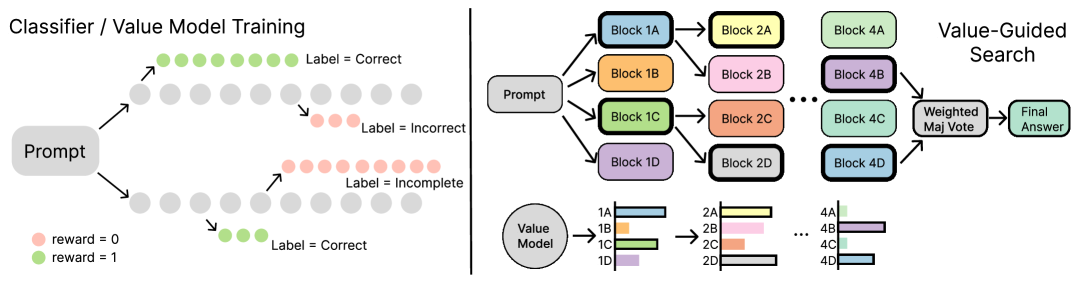
Figure 2: Summary of Methods. (Left) Diagrams how we collect multiple roll-ins (grey circles representing tokens) per problem, and branch off multiple roll-outs per roll-in at random points. The class label for each roll-out token is the outcome label at the very end. (Right) Shows the beam search process (beam width $2$ and budget $4$) guided by a value model.

2.1 Learning Algorithm for Value Model

We describe our training process for a language value model by performing regression via classification [7]. Let $\mathcal{V}$ be the vocabulary and let $\mathcal{S}=\bigcup_{n\in\mathbb{N}}\mathcal{V}^{n}$ denote the input sequence space. Given a problem prompt $x\in\mathcal{S}$ and a response $y\in\mathcal{S}$, let $\kappa=\Gamma(x,y)\in[0,1,\dots,K-1]$ denote its class label, where $K$ is the number of classes. Furthermore, let $r=R(x,y)$ denote the scalar reward, which we assume to be binary since we focus on competition math (see Appendix˜B for the general case). For our value model, $\kappa=2$ if the response is an incomplete generation (i.e., exceeds max generation length), $\kappa=0$ if the response finished and is incorrect, and $\kappa=1$ if the response finished and is correct. Thus, the event that $\kappa=1$ corresponds to $r=1$ (correct answer), and $\kappa\in\{0,2\}$ corresponds to $r=0$ (incorrect or exceeds max length). We adopt this convention in the rest of the paper. We remark that regression-via-classification is a standard approach that leads to better down-stream decision making than regressing via squared error [7, 20, 17, 3, 42, 43].

We employ datasets of the form $\mathcal{D}=\{(x_{i},y_{i},z_{i},\kappa_{i})\}_{i\in[N]}$, where $x_{i}$ is the problem prompt, $y_{i}$ is a partial response (which we call a “roll-in”), $z_{i}$ is a completion starting from $y_{i}$ (which we call a “roll-out”), and $\kappa_{i}=\Gamma(x_{i},y_{i},z_{i})$ is the label of the full response, where $x,y,z$ denotes the concatenation of $x$, $y$ and $z$. In this paper, we assume that the completions / roll-outs $z_{i}$ are generated by a fixed roll-out policy $\pi^{\text{ref}}$, i.e., $z_{i}\sim\pi^{\text{ref}}(\cdot\mid x_{i},y_{i})$ for all $i$. We remark that a good choice for $\pi^{\text{ref}}$ is a cost-efficient model which is capable of producing diverse responses with positive reward, e.g., a distilled version of a large reasoning model.

We train a classifier $f_{\theta}:\mathcal{S}\mapsto\Delta([K])$ via gradient descent on the following loss on data batch $\mathcal{B}$:

$$L(\theta;\mathcal{B}) \textstyle=\frac{1}{|\mathcal{B}|}\sum_{(x_{i},y_{i},z_{i},\kappa_{i})\in\mathcal{B}}\frac{1}{|z_{i}|}\sum_{h\in\operatorname{range}(|z_{i}|)}\ell_{\operatorname{ce}}(f_{\theta}(x_{i},y_{i},z_{i}^{:h}),\kappa_{i}),$$

where $\ell_{\operatorname{ce}}(\hat{p},\kappa)=-\ln(\hat{p}[\kappa])$ is the standard cross-entropy loss for classification and $z_{i}^{:h}$ denotes the first $h$ tokens of $z_{i}$. The rationale for the inner average is analogous to next-token prediction training of autoregressive models: since $z_{i}$ is generated autoregressively by $\pi^{\text{ref}}$, any suffix $z_{i}^{h:}$ is also a roll-out from $\pi^{\text{ref}}$ and hence can be viewed as another data-point. We found this to be an important training detail for performance, which is consistent with prior work who used a similar objective for training an outcome reward model [14, 23].

We can now view the classifier as a value model. Since $\kappa=1$ corresponds to the event that $r=1$, we have that $V_{\theta}(x):=f_{\theta}(x)[1]$ predicts the correctness probability of roll-outs from $\pi^{\text{ref}}$. Indeed, if $f^{\star}$ denotes the optimal classifier that minimizes the population-level loss, then $f^{\star}(x,y)[1]=\mathbb{E}_{z\sim\pi^{\text{ref}}(\cdot\mid x,y)}[R(x,y,z)\mid x,y]$ which is the expected reward of a completed response from rolling-out $\pi^{\text{ref}}$ starting from $x,y$. In sum, our value model is learned via predicting labels (one of which corresponds to reward $1$), and the training objective is the standard cross-entropy loss.

2.2 Dataset Creation Process

We describe our process for creating OpenR1-VM, a novel dataset of 2.5 million reasoning responses from DeepSeek models, across 45k math problems from OpenR1-Math [2].

Pre-Filtering. We start from the OpenR1-Math dataset (default split) [2] which contains 94k math problems with solutions that were already filtered for quality. Upon manual inspection, we found that this dataset still contained unsolvable problems (e.g., problems that require web browsing but our models cannot access the web) and ambiguous or unverifiable answers (e.g., multiple \boxed{} expressions or unparsable answers). We filter out all such problematic problems, producing a cleaned subset of 50k problems with solutions verifiable by sympy or math-verify [22]. We call this pre-filtered dataset OpenR1-Cleaned.

Response Generation. Next, we collect roll-ins and roll-outs from DeepSeek models [18]. We fix the roll-out policy $\pi^{\text{ref}}$ as DeepSeek-R1-Distill-Qwen-1.5B. To ensure diversity in the roll-in distribution, we sample $14$ independent roll-ins from four DeepSeek-R1-Distill-Qwen model sizes: 1.5B, 7B, 14B, and 32B by generating until the end of thinking token <\think>. For each roll-in $\tilde{y_{i}}$, we then sample four random prefix locations where we generate complete roll-outs $\{z_{i}^{j}\}_{j\in[4]}$ from $\pi^{\text{ref}}$. Finally, to compute the class label (incomplete, incorrect, or correct), we parse the response for the final answer (enclosed in \boxed{}) and use math-verify to check for correctness against the ground truth answer. In total, this process (illustrated in Fig.˜2 left) yields $56$ labeled roll-in, roll-out pairs per problem, leading to 2.8 million datapoints.

Post-Filtering. We filter out problems where all $56$ roll-outs for that problem were incomplete or incorrect (i.e., has reward $0$). This post-filtering removes any ambiguous or unanswerable problems that we missed during pre-filtering, and also removes problems that are too difficult for $\pi^{\text{ref}}$ and do not provide a useful learning signal. This step filters roughly $10\%$ of problems, yielding a final dataset of 2.5 million datapoints.

Notably, our approach does not require a fine-grained notion of step and our data collection is cheaper than existing PRM techniques. Specifically, Lightman et al. [23] used per-step annotations by human experts, Zhang et al. [50] used per-step annotations via LLM-as-a-Judge, and Wang et al. [44] used multiple Monte Carlo roll-outs at every step. Since the number of newlines in reasoning CoT traces can grow very quickly, per-step labels are quite expensive to collect for reasoning models. In contrast, our approach only requires a handful of roll-ins (from any policy) and roll-outs (from $\pi^{\text{ref}}$) per problem, and this number can be flexibly tuned up or down to trade-off data coverage and data collection cost. Please refer to Appendix˜D for further details on each step. We also release our filtering code and datasets to support future research.

Algorithm 1 Beam Search with Width $w$

1:Input: prompt $x$.

2:Set num beams $B\leftarrow\frac{N}{w}$.

3:Initialize beams $y_{1},\dots,y_{B}\leftarrow x$.

4:while $\exists j$ s.t. $y_{j}$ is not finished do

5:  For each $j$ s.t. $y_{j}$ is not finished, sample $w$ i.i.d. blocks $\{b_{i,j}\}_{i\in[w]}$ from $\pi(\cdot\mid y_{j})$.

6:  Update unfinished beams to be the best continuations with the highest $V(y_{j},b_{i,j})$.

7:end while

8:return BoN or WMV on $\{y_{1},\dots,y_{B}\}$.

Algorithm 2 Best-of-$N$

1:Input: prompt $x$, responses $\{y_{i}\}_{i\in[N]}$.

2:return $y^{\text{bon}}=\mathop{\rm arg\,max}_{y_{i}}V(x,y_{i})$.

Algorithm 3 (Weighted) Majority Vote

1:Input: prompt $x$, responses $\{y_{i}\}_{i\in[N]}$, weights $\{w_{i}\}_{i\in[N]}$, equivalence relation $\sim$.

2:Partition $\{y_{i}\}_{i}$ into equiv. classes $\{p_{k}\}_{k}$.

3:return A response from the highest weight partition $\mathop{\rm arg\,max}_{p_{k}}\sum_{y_{i}\in p_{k}}w_{i}$.

2.3 Algorithms for Test-Time Compute and Search

Equipped with a value model $V:\mathcal{S}\mapsto\mathbb{R}$, we can now apply it to scale test-time compute of a generator model $\pi$. For search-based approaches, we focus on block-wise search where a “block” refers to a sequence of tokens (e.g., blocks of $4096$ tokens worked best in our experiments). We let $N$ denote the inference budget, which is the number of generations we can sample (e.g., generating four responses and taking a majority vote is $N=4)$.

BFS. Breadth-first-search (BFS) [47, 28] is a natural search method that approximates the optimal KL-regularized policy given a good value model [52]. Given a prompt $x$, BFS samples $N$ parallel blocks $b_{i}$ from $\pi$ and selects the block with the highest value $b^{\star}=\mathop{\rm arg\,max}_{b_{i}}V(x,b_{i})$, which gets added to the prompt, i.e., $x\leftarrow x,b^{\star}$. The process repeats until the response finishes. Note the number of tokens generated from $\pi$ is roughly equivalent to $N$ independent generations from $\pi$.

Beam Search. One weakness of BFS is that parallel blocks are correlated because they share the same prefix, which limits diversity. Beam search with width $w$ (Algorithm˜1) is a generalization that keeps $B=N/w$ (assume to be integer) partial responses and branches $w$ parallel blocks from each one [26, 5, 40, 6, 36]. Given a prompt $x$, beam search first generates $N$ parallel blocks. However, unlike BFS, beam search keeps the top $B$ beams with the highest scores, and then samples $w$ parallel blocks per beam at the next step. Since $B\times w=N$ blocks are sampled at each step, the compute budget is also $N$. We illustrate beam search with $N=4$ and $w=2$ in Fig.˜2 (right).

DVTS. Diverse verifier tree search (DVTS) is a meta-algorithm that further increases diversity by running parallel searches each with smaller budgets [6]. Specifically, DVTS-$M$ runs $M$ parallel beam searches each with budget $N/M$ (assume to be integer), and aggregates responses into a final answer.

We remark a crucial detail of beam search and DVTS is how the final set of beams/responses are aggregated. Prior works [6, 36, 34] select the response with the highest score, which is analogous to a final best-of-$N$ (BoN; Algorithm˜2). Instead, we found that taking a weighted majority vote (WMV; Algorithm˜3) led to much better performance, which is demonstrated by Fig.˜3 (left).

Computational Efficiency of Block-wise Search. Since value scores are only used at the end of each block or the end of the whole response, the FLOPs required for block-wise value model guidance is a tiny fraction ($\ll 1\%$) of the generation cost from $\pi$. We compute FLOP estimates in Appendix˜H to concretely show this.

3 Experiments

We extensively evaluate value-guided search (VGS) with our 1.5B value model DeepSeek-VM-1.5B, focusing on guiding the CoT reasoning of DeepSeek models [18]. The best VGS setup for our value model is beam search with final WMV aggregation, beam width 2, block size 4096 and with DVTS (for larger inference budgets). We show this setup outperforms other test-time compute methods (e.g., MV, WMV, BoN) and other scoring models (e.g., existing 7B PRMs and a 1.5B Bradley-Terry reward model trained on our dataset). We remark our search results use a fixed beam width and block size for all problems; this is more practical than prior works on “compute-optimal scaling” which vary search parameters for each problem and require estimating each problem’s difficulty [6, 36, 25]. Please see Appendices˜E and F for additional details on value model training and inference.

Benchmarks. We evaluate on the 2024 and 2025 editions of the American Invitational Mathematics Exam (AIME) and the February Harvard-MIT Mathematics Tournament (HMMT). Both AIME and HMMT are prestigious high school math competitions in the US that have also been used to evaluate frontier LLMs [31, 18, 1]. We use AIME I & II and the individual part of HMMT, yielding $30$ problems per competition. To mitigate overfitting on a single widely used benchmark, we report the overall averaged accuracy unless otherwise stated. Per-benchmark plots are relegated to Appendix˜C.

Baseline Models. We evaluate two state-of-the-art 7B PRMs with distinct training styles: Math-Shepherd-Mistral-7B-PRM [44] and Qwen2.5-Math-PRM-7B [50]. Math-Shepherd uses Monte-Carlo roll-outs from each step to estimate per-step value while the Qwen2.5 PRM uses LLM-Judge annotation for each step, similar to the per-step human annotation of PRM800K [23]. As a step-level value model, Math-Shepherd-PRM-7B is more related to our token-level value model. Finally, we also evaluate a 1.5B Bradley-Terry (BT) [8] model, called DeepSeek-BT-1.5B, which we trained using our dataset (see Appendix˜G for training details).

Test-time scaling DeepSeek-1.5B ($N=256$)	AIME-24	AIME-25	HMMT-24	HMMT-25	AVG
VGS w/ DeepSeek-VM-1.5B (ours)	$72.0\pm 0.4$	$46.7\pm 0.7$	$31.4\pm 2.0$	$32.8\pm 0.8$	$\mathbf{45.7\pm 1.0}$
WMV w/ DeepSeek-VM-1.5B (ours)	$69.6\pm 3.9$	$45.1\pm 2.2$	$29.1\pm 2.6$	$28.9\pm 2.6$	$43.2\pm 1.4$
VGS w/ DeepSeek-BT-1.5B (ours)	$73.1\pm 1.4$	$40.6\pm 0.8$	$28.1\pm 1.9$	$27.5\pm 0.0$	$42.3\pm 0.5$
WMV w/ DeepSeek-BT-1.5B (ours)	$72.0\pm 3.3$	$40.5\pm 2.9$	$25.3\pm 2.3$	$24.6\pm 4.7$	$40.6\pm 1.6$
VGS w/ Qwen2.5-Math-PRM-7B	$71.1\pm 1.0$	$38.9\pm 1.4$	$26.7\pm 1.2$	$24.2\pm 0.2$	$40.2\pm 0.5$
WMV w/ Qwen2.5-Math-PRM-7B	$70.6\pm 3.1$	$39.1\pm 2.1$	$25.4\pm 2.4$	$24.0\pm 3.2$	$39.8\pm 1.4$
VGS w/ MathShepherd-PRM-7B	$70.6\pm 3.1$	$41.9\pm 1.4$	$30.0\pm 1.4$	$23.9\pm 1.4$	$41.6\pm 0.9$
WMV w/ MathShepherd-PRM-7B	$71.2\pm 3.2$	$40.0\pm 2.5$	$27.9\pm 2.3$	$25.6\pm 3.1$	$41.2\pm 1.4$
MV@256	$71.0\pm 3.5$	$38.9\pm 1.9$	$24.4\pm 1.7$	$24.3\pm 2.9$	$39.7\pm 1.2$
Test-time scaling larger models with our DeepSeek-VM-1.5B
VGS w/ DeepSeek-7B ($N=128$)	$82.2\pm 0.8$	$59.4\pm 0.8$	$42.8\pm 2.8$	$41.1\pm 1.6$	$\mathbf{56.4\pm 0.8}$
MV w/ DeepSeek-7B ($N=128$)	$77.1\pm 1.1$	$56.5\pm 1.6$	$34.7\pm 1.6$	$33.8\pm 2.5$	$50.5\pm 0.9$
VGS w/ DeepSeek-14B ($N=64$)	$86.7\pm 2.7$	$59.6\pm 0.6$	$46.7\pm 2.7$	$51.1\pm 1.6$	$\mathbf{61.0\pm 0.9}$
MV w/ DeepSeek-14B ($N=64$)	$80.6\pm 1.2$	$67.0\pm 2.0$	$40.6\pm 1.8$	$50.1\pm 2.0$	$59.6\pm 0.9$
Pass@N baselines for various models
DeepSeek-1.5B Pass@1	$28.2\pm 6.1$	$22.4\pm 4.1$	$13.9\pm 4.2$	$13.0\pm 3.9$	$19.4\pm 1.1$
DeepSeek-32B Pass@1	$77.2\pm 4.9$	$60.4\pm 6.0$	$38.0\pm 4.6$	$42.1\pm 5.2$	$54.4\pm 1.3$
Deepseek-R1 (671B) Pass@1	$85.0\pm 2.1$	$70.0\pm 0.9$	$41.7\pm 3.5$	$46.7\pm 2.4$	$\mathbf{60.8\pm 0.5}$
o3-mini-medium Pass@1	$49.2\pm 6.8$	$45.8\pm 6.6$	$32.4\pm 5.4$	$36.6\pm 6.0$	$41.0\pm 1.5$
o3-mini-medium Pass@8	$83.0\pm 4.6$	$77.4\pm 3.9$	$55.9\pm 4.3$	$64.9\pm 4.4$	$\underline{70.3\pm 2.1}$
o4-mini-medium Pass@1	$85.4\pm 4.3$	$82.3\pm 4.5$	$50.4\pm 5.0$	$61.1\pm 6.4$	$69.8\pm 2.5$
o4-mini-medium Pass@8	$95.4\pm 2.6$	$93.3\pm 0.4$	$69.7\pm 3.2$	$84.5\pm 2.5$	$\mathbf{85.7\pm 1.1}$

Table 1: (Top) Weighted majority vote (WMV) and VGS results for DeepSeek-1.5B with an inference budget of $N=256$, using various scoring models. (Middle) Compares MV and VGS for larger DeepSeek models guided with our DeepSeek-VM-1.5B. (Bottom) Lists performance of DeepSeek models and strong close-sourced reasoning models. For VGS, $\pm$ indicates standard deviation across 3 seeds; for MV, WMV, Pass@N, $\pm$ denotes bootstrap with $100$ repetitions. We bold the highest avg. accuracy and underline second highest. Section˜C.1 contains more baselines.

3.1 Main Results (Table˜1)

In the top section of Table˜1, we fix the generator to DeepSeek-1.5B and test-time budget to $N=256$, and compare VGS to weighted majority voting (WMV), using our value model, the BT model and baseline PRMs. We see that VGS and WMV with DeepSeek-VM-1.5B achieve the two highest scores, outperforming the BT reward model and prior PRMs. This shows that our value model is not only a strong outcome reward model (ORM) but also an effective value model for guiding search. Notably, with a budget of $256$, our 1.5B value model can guide DeepSeek-1.5B (total parameter count is 3B) to reach parity with the pass@1 of o3-mini-medium, a strong math reasoning model from OpenAI. Intriguingly, while DeepSeek-BT-1.5B was only trained as an ORM, we find that VGS also improves performance relative to WMV, suggesting that BT models may also provide meaningful block-wise feedback to guide search. We also observe that accuracies for the 7B baseline PRMs (MathSheperd and Qwen2.5-Math) are only slightly higher than MV@256 and do not improve with search, which suggests that these PRMs are likely out-of-distribution (OOD) for the long CoTs generated by DeepSeek-1.5B.

In the middle section of Table˜1, we guide stronger DeepSeek models with sizes 7B and 14B, and compare VGS to MV, a standard TTC method that does not use an external scoring model. We see that VGS again achieves higher accuracy than MV for both 7B and 14B, which suggests that DeepSeek-VM-1.5B is also useful in guiding the CoT of stronger DeepSeek models. However, we observe that the gap between VGS and MV becomes smaller for larger DeepSeek models, suggesting that DeepSeek-14B CoTs may be becoming OOD for our value model, which was trained on DeepSeek-1.5B CoTs. To guide more capable models, new value models should be trained on rollouts from similarly capable models; we however do not foresee this being a practical concern given the scalability of our training process (described in Section˜2 and summarized in Appendix˜B). Finally, we note that the performance of all models on AIME-24 is consistently higher than other competitions, suggesting the importance of evaluating on diverse and newer competitions to reduce risk of overfitting or data contamination.

3.2 Test-Time Compute Scaling for Search

This section presents three experiments designed to analyze the TTC scaling properties of VGS. Our investigation addresses three key research questions:

1. Does VGS, with its block-wise guidance, demonstrate superior performance compared to response-level aggregation methods such as BoN or WMV?

2. How does the TTC scaling behavior of VGS compare to the standard score-free baseline MV?

3. How does the TTC scaling behavior of DeepSeek-VM-1.5B compare to baseline models?

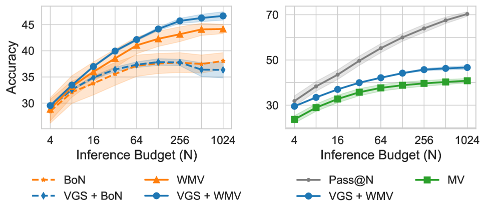
Figure 3: Test-Time Compute with DeepSeek-VM-1.5B. (Left) Compares best-of-$N$ (BoN), weighted majority voting (WMV) and VGS with either BoN or WMV for the final aggregation. (Right) Compares VGS to majority voting (MV), a standard baseline that does not require a scorer.

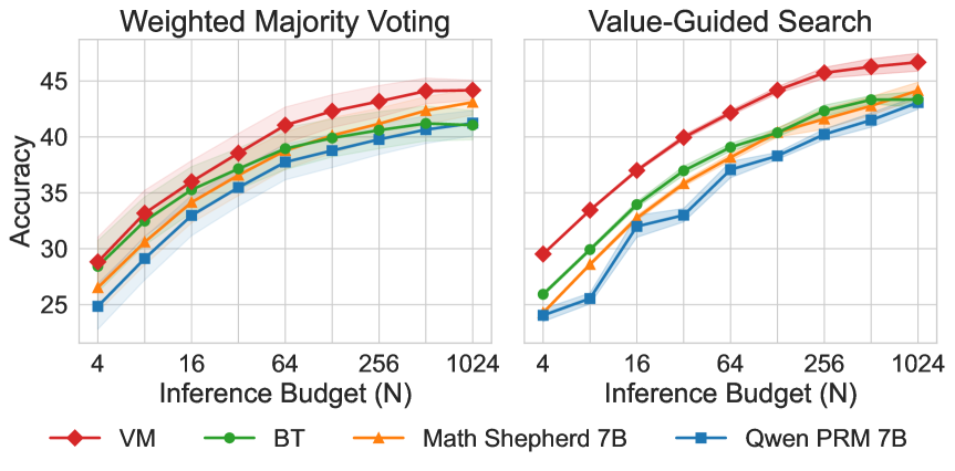
Figure 4: TTC Scaling of Various Scorers. Comparison of our 1.5B value model (VM), our 1.5B Bradley-Terry reward model (BT), and two 7B state-of-the-art PRMs for two TTC scaling methods: (Left) WMV or (Right) VGS (with WMV as a final aggregation step).

Response-Level Selection vs Search-Based Block-Level Selection. While BoN and WMV represent standard approaches for selecting responses using an ORM, block-wise VGS guides response generation through sequential block-by-block selection. As Fig.˜3 (left) illustrates, WMV consistently outperforms BoN across all inference budget scales, which demonstrates the benefits of combining MV with value scores. Furthermore, VGS (with WMV as a final aggregation step) yields additional improvements beyond WMV alone. This confirms the benefits of search and aligns with conclusions from previous studies [6, 36, 25]. Interestingly, we do not observe the same benefits of search if BoN is used as a final aggregation step, suggesting that WMV is a critical component to VGS.

Response Length for VGS. In addition to consistent performance gains, VGS also produces noticeably shorter responses compared to the base DeepSeek-1.5B model. In Figure 15 (Appendix C.7), we present histograms of response lengths across all benchmarks. The results show that VGS consistently generates more concise outputs, whereas the base model often reaches the generation cap, with up to 50% of its responses being unfinished. On average, VGS responses are 11,219 tokens long, compared to 12,793 for DeepSeek-1.5B, representing a reduction of over 12% in token and thus FLOPs usage.

VGS vs Majority Voting. As Fig.˜3 (right) demonstrates, VGS consistently achieves higher accuracy than MV, attaining equivalent performance while requiring substantially lower inference budgets (also shown in Fig.˜1 right). Fully closing the gap with the oracle Pass@N curve may require a larger value model trained on more extensive datasets.

DeepSeek-VM-1.5B vs Baseline Scoring Models. Fig.˜4 benchmarks DeepSeek-VM-1.5B against existing PRMs and our BT model. We observe that DeepSeek-VM-1.5B consistently delivers superior performance when employed both as an ORM for WMV (left) and as a guidance mechanism for block-wise search (right). Note that we find our BT model to be surprisingly effective as a search guidance model which suggests the importance of our token-level dataset playing an important role in successful downstream search.

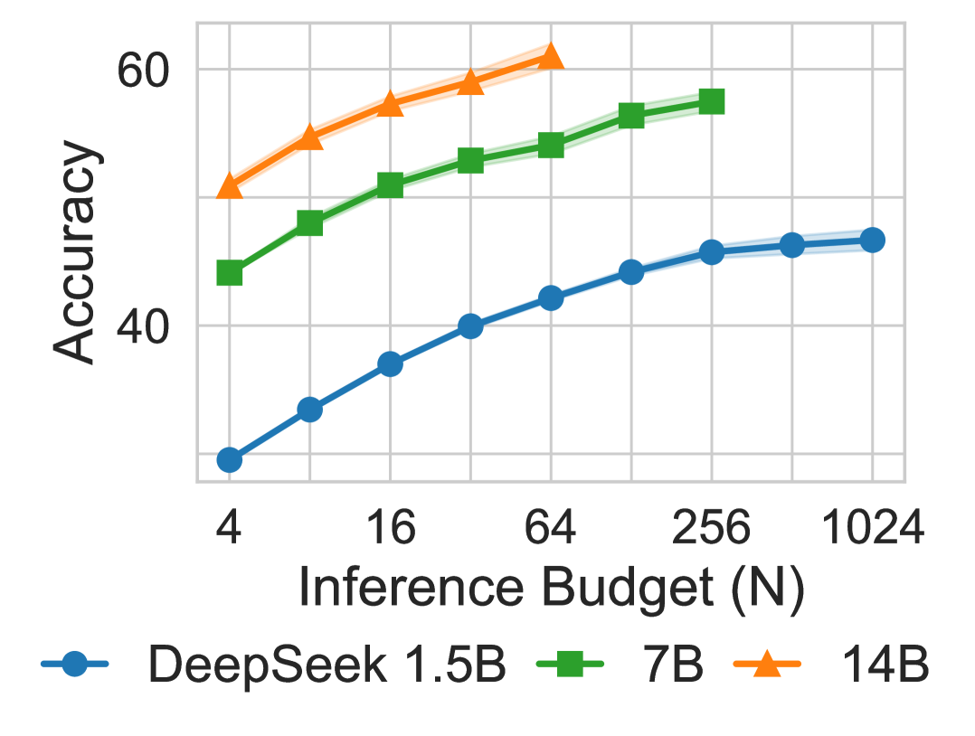
Figure 5: VGS + WMV Performance when Guiding Larger Models. With the same DeepSeek-VM-1.5B providing guidance, search continues to improve with more test-time compute.

3.3 Scaling up the Generator Model Sizes

In Fig.˜5, we scale up our experiments to guide larger 7B and 14B DeepSeek models. Here, we run VGS with the same search parameters using the same value model DeepSeek-VM-1.5B. Although the 7B and 14B DeepSeek models are in theory OOD for our value model [52], which was trained on DeepSeek-1.5B rollouts, we observe that VGS continues to scale without plateauing as test-time compute increases. This provides some evidence that a value model trained with a weaker verifier policy can generalize effectively and guide the CoTs of stronger models. Such generalization is particularly valuable, as it is significantly cheaper to collect training data from smaller $\pi^{\text{ref}}$ models. This form of “weak-to-strong” generalization [10] appears to be a promising direction for future research.

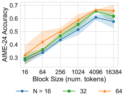
Figure 6: Ablation: Search Block Size. AIME-24 accuracies for beam search (width $2$) with varying block sizes from 16 to 16384. We found 4096 to be optimal across test-time budgets and benchmarks.

4 Ablation Studies

To investigate the role of key hyperparameters in search, we perform sensitivity analyses of block size and beam width on AIME-24 across varying inference budgets. We also ablate the amount of DVTS parallelism. These tests suggest that there is a consistent choice of search hyperparameters that work well across inference budgets.

4.1 Different Search Parameters and Methods

Block Size. We perform beam search with width $2$ using search block sizes from 16 to 16384. Fig.˜6 shows AIME-24 accuracies across three inference budgets $N$, revealing that the optimal choice of $4096$ stays consistent across different $N$. We see a decline in performance when searching with more fine-grained blocks.

Beam Width. We perform beam search with block size $4096$ using varying beam widths, with breadth-first-search (BFS) being a special case where beam width is equal to $N$. Fig.˜7 (left) shows AIME-24 accuracies across five inference budgets, demonstrating that beam width $2$ is consistently optimal across different $N$. We note our optimal beam width is different from prior works’ which found $4$ to work best [6, 36, 25].

DVTS Parallelism. Fig.˜7 (right) shows the role of ablating DVTS from VGS. For each inference budget, we report average accuracies without DVTS and with the best DVTS parallelism $M$. We observe that DVTS becomes more effective at higher budgets and scales better than a single search tree, which is consistent with findings from prior works [6]. However, we find that DVTS is never worse than a single search tree even at smaller inference budgets, which is the opposite conclusion reached by prior works [6]. This discrepancy may be explained by the fact that we use WMV to combine the DVTS responses, which seems to be a more robust way to perform DVTS than BoN (used in prior works) given our findings from Fig.˜3.

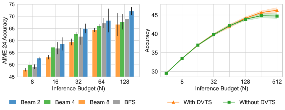
Figure 7: Ablations: Beam-Width and DVTS. (Left) AIME-24 accuracies for beam search with various widths (Section˜2.3) across inference budgets $N$. BFS is equivalent to setting width as $N$. We find that the optimal beam width is robust across multiple TTC budgets. (Right) Averaged accuracy for beam $2$ with and without DVTS. For DVTS, we report the best result with parallelism $M>1$ per inference budget $N$, which we find scales better at higher budgets.

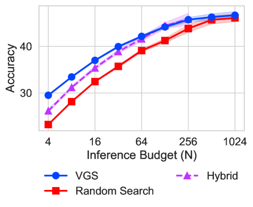
Figure 8: Ablation: Random Search. Random search is the same search process as VGS except intermediate blocks are randomly selected instead of using our value model. Hybrid is a mixture where we flip a fair coin at the start of a search tree that decides whether to use random search or VGS. We see that selecting blocks with highest value improves accuracy across inference budgets.

4.2 Random vs. Value-Guided Search

Finally, we directly ablate the role of our value model’s guidance during the search process. We perform VGS (w/ same width, block size and DVTS) but randomly select blocks instead of selecting blocks with the highest value. We still aggregate the final beams via WMV with our value model, so the only change is how intermediate blocks are chosen. We call this process “random search”. Thus, if our value model is helpful for search, we should expect VGS to outperform random search. Indeed, Fig.˜8 validates this hypothesis. We also evaluate a hybrid approach where half of DVTS’s parallel trees use random search and the other half use VGS. We find that this hybrid approach lands roughly between pure VGS and pure random search, again validating that block-selection from our value model improves over random selection.

5 Conclusion

In this paper, we introduced block-wise Value-Guided Search (VGS), a simple yet effective strategy for steering long-context CoT reasoning models. We proposed a scalable token-level value model training pipeline that does not require a pre-defined notion of “step” or expensive per-step annotations. We collect a large dataset of reasoning CoTs (OpenR1-VM) and train a lean 1.5B value model (DeepSeek-VM-1.5B), which we show can effectively guide the CoTs of DeepSeek models up to 14B in size. With extensive experiments, we demonstrate that VGS with DeepSeek-VM-1.5B enjoys better test-time compute scaling than standard methods (e.g., majority voting, best-of-$N$) and other scoring models (e.g., existing PRMs and a BT model), achieving a higher performance ceiling while reducing the FLOPs needed to extract the same performance as baseline methods (Fig.˜1). Our results point to VGS as a promising approach to scale TTC of emerging reasoning models.

Discussion of Limitations. Our value model is trained exclusively on completions / roll-outs from a lean reasoning model $\pi^{\text{ref}}$ (e.g., DeepSeek-R1-Distill-Qwen-1.5B). As frontier LLMs continue to advance, the distribution of their generated responses may increasingly diverge from our training distribution, potentially degrading scoring and search performance. To maintain optimal performance, new value models will need to be retrained on rollouts from updated generator policies. However, we do not foresee this as a major practical concern given the simplicity and scalability of our pipeline. To facilitate retraining and adaptation to similar verifiable domains, we open-source our codebase and provide a step-by-step recipe in Appendix˜B for data collection, training and search inference.

Appendices

Table of Contents

• Appendix A. Related Works

• Appendix B. Summary of VGS Pipeline

• Appendix C. Additional Experiment Results

• Appendix D. Further Details of Data Collection

• Appendix E. Further Details for Value Model Training

• Appendix F. Further Details for Inference with Search

• Appendix H. Inference FLOPS Computation

Note: In the appendix, we also provide additional empirical results in Appendix˜C. Two new results are worth highlighting here. First, in Section˜C.6, we provide test-time scaling results for guiding DeepSeek-1.5B further trained with PPO on our math dataset. We find that VGS improves test-time scaling compared to MV and WMV, which shows that our method nicely complements policy-based RL training. Moreover, in Section˜C.7, we include three qualitative examples of contrastive blocks that were selected or rejected by our value model during beam search process. We see that our value model prefers blocks with more straightforward logical deductions, yielding more efficient and effective CoT for reasoning.

Appendix A Related Works

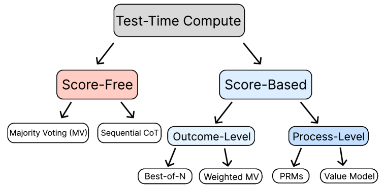
Figure 9: Taxonomy of TTC Methods. Score-free TTC methods do not require an external scoring model, e.g., by taking a majority vote. Score-based TTC methods require an external scoring model. The coarsest scoring model is an outcome reward model (ORM), which scores a whole response and can be used for best-of-$N$ or weighted MV. A more fine-grained scoring model are process-level scorers, which includes process reward models (PRMs) and value models; these more fine-grained scoring models can be used for search.

Test-time compute (TTC) broadly refers to algorithms that improve problem-solving performance when given more compute (i.e., FLOPs) at test-time. Fig.˜9 summarizes the taxonomy of TTC methods. The simplest TTC methods are score-free in the sense that they do not require access to an external scoring model. A notable example is majority voting (MV), which selects the most frequent answer among $N$ responses, breaking ties randomly [14, 46, 9]. Also known as self-consistency, MV can be applied to tasks where the output space is equipped with an equivalence relation, e.g., mathematical formulae that can be symbolically checked for equality. Other score-free TTC methods include sequentially revising the response via CoT prompting [38, 29] and hybrid methods [41].

There are also score-based TTC methods that employ an external scorer. The coarsest type of a scorer is an outcome reward model (ORM), which takes the full prompt and response as input and produces a scalar that measures the quality / correctness of the response. Popular examples of ORMs include Bradley-Terry reward models [8] or LLM-as-a-Judge [4]. ORMs can be used for best-of-$N$ (BoN), which selects the response with the highest score [14, 4]. ORMs can also be used for weighted majority voting (WMV), which generalizes MV where the strength of a response’s vote is proportional to its ORM score. Weighted MV (WMV) typically provides an improvement over vanilla (unweighted) MV [6, 25], which is also what we observe in our experiments (Fig.˜3).

Outcome-level TTC methods (e.g., BoN, WMV) may be further refined with process-level scorers that guide the generation process in a fine-grained manner. We remark that our value model can act as both an outcome-level and a process-level scorer. When queried with a partial response, the value model predicts the expected quality of future completions under $\pi^{\text{ref}}$. When queried at the end of a full response, the value model predicts the quality of the final response. Indeed, our best performing setup for value-guided search (VGS) uses intermediate values to guide block-wise beam search and uses final values via WMV to aggregate the final beams, which employs both the process-level and outcome-level scoring capabilities of the value model. Finally, to the best of our knowledge, the combination of search with WMV is novel to this work, and we found this to be a crucial ingredient to effectively scale TTC of DeepSeek models.

Prior works on process-level TTC largely focused on step-wise search with process reward models (PRMs), which measures the correctness of a fine-grained step [23]. They showed that step-wise search can provide better performance than outcome-level TTC methods [28, 47, 24, 36, 48, 34, 13]. However, training step-wise PRMs requires a pre-defined notion of step, which is challenging to explicitly define for general reasoning [18]; e.g., prior works used newlines \n to separate steps, but DeepSeek’s CoTs often contain newlines in-between coherent thoughts. Moreover, prior PRM training techniques require per-step annotations, via humans [23], LLM-Judges [50], or per-step MC rollouts [44, 27], which are expensive to collect for long reasoning traces; e.g., a single response from DeepSeek models typically contains hundreds of newlines.

These limitations make it difficult to scale PRMs to long-context reasoning models [18], and all these prior works could only evaluate on short-context models with easier benchmarks such as GSM8k [14] and MATH [23]. In contrast, our paper focuses on scaling process-level guidance to long-context reasoning models, and we propose a block-level search method that mitigates the above limitations. We train a token-level value model by collecting rollouts from random solution prefixes, which requires neither a pre-defined notion of step nor per-step annotations. We use our value model to guide a block-wise search process, where the block size is a hyperparameter and we find there exists a consistent choice that works well across inference budgets (Fig.˜6). Crucially, we are able to scale our value-guided search (VGS) to long-context DeepSeek models and demonstrate impressive performance and efficiency gains on challenging math competitions (Fig.˜1).

Closely related to our work is Setlur et al. [34], who propose to train a token-level process advantage verifier (PAV), which is the sum of $\pi^{\text{ref}}$’s $Q$-function and an (off-policy) expert’s advantage function, to guide step-wise search. This method is similar to ours since the training process also occurs at a token-level and is agnostic to the definition of step. However, a limitation of the PAV is that if the expert disagrees with the underlying policy, then maximizing the PAV can lead to suboptimal behavior [12]. Our approach of directly using the value model does not have this issue. Moreover, Setlur et al. [34] proposed to use PAVs to guide step-wise search, which still requires a definition of step at inference time; in contrast, we propose to use block-wise search which does not require a definition of step at inference. At a technical level, Setlur et al. [34] trained the PAV by minimizing the mean-squared error (MSE) loss; in contrast, we propose to use the cross-entropy loss, which has been shown to work better for downstream decision making [17, 43, 52].

We remark that some prior works proposed to use token-level value models to reweight the next-token distribution of the generator [28, 49, 19, 52]. However, these methods require one classifier call per token, which is more expensive than block-wise search. Moreover, token-level guidance might also be less effective because the imperfect value model may introduce cascading errors if queried at every token. We highlight that Mudgal et al. [28] also experimented with block-wise BFS and found this to be more effective at scaling test-time compute than reweighting the next-token distribution (i.e., token-wise guidance). One drawback of block-wise BFS is that the blocks may all become correlated due to sharing the same prefix. Thus, we build upon Mudgal et al. [28] by proposing to use beam search, which we show yields better test-time scaling for reasoning models (Fig.˜6).

Appendix B Summary of VGS Pipeline

We provide a step-by-step recipe for running VGS on any verifiable domain of interest. This recipe is applicable to any task with a reward label for responses (i.e., outcome-level feedback). If the task has continuous rewards, a standard trick from distributional RL is to discretize the reward distribution as a histogram, and then the value model is simply the expected reward under the learned distribution [7, 20, 17, 42, 43].

1. Start with a verifiable domain, where responses are identified with a label and a reward.

2. Identify a good dataset of prompts.

3. Identify a set of roll-in policies and a single roll-out policy. The roll-in policies should provide a diverse distribution of solutions, and the roll-out policy should be strong enough to complete responses given a partial roll-in.

4. For each prompt, sample $n$ roll-in responses from the set of roll-in policies.

5. For each roll-in response, sample $m$ random indices $\{i_{j}\}_{j\in[m]}$, and collect a roll-out per index. Thus, there are $nm$ roll-in, roll-out pairs per prompt.

6. Post-filter by removing prompts where all roll-out responses fail to complete or solve the prompt.

7. At this point, we have created our dataset of roll-in, roll-out pairs. We are now ready to train our value model.

8. Train a classifier / value model by following (Section˜2.1). Sweep hyperparameters such as learning rate.

9. Choose a generator policy to be guided by the value model. The most in-distribution choice is to use the roll-out policy $\pi^{\text{ref}}$.

10. Perform model selection by running outcome-level TTC (e.g., WMV) on some validation benchmark.

11. Sweep search parameters (e.g., block size, beam width, DVTS parallelism) on the validation benchmark.

12. Run the final model on the test benchmark with the best search parameters.

The sampling distribution for the cut-off index (Step 5) is also worth tuning. For example, values at earlier or middle indices may be harder to predict than final indices, so it is worth sampling more cut-off indices from these earlier regions.

Appendix C Additional Experiment Results

C.1 Full Main Results Table

We reproduce Table˜1 with additional baselines: DeepSeek-7B, DeepSeek-14B, o1-mini-medium.

Test-time scaling DeepSeek-1.5B ($N=256$)	AIME-24	AIME-25	HMMT-24	HMMT-25	AVG
VGS w/ DeepSeek-VM-1.5B (ours)	$72.0\pm 0.4$	$46.7\pm 0.7$	$31.4\pm 2.0$	$32.8\pm 0.8$	$\mathbf{45.7\pm 1.0}$
WMV w/ DeepSeek-VM-1.5B (ours)	$69.6\pm 3.9$	$45.1\pm 2.2$	$29.1\pm 2.6$	$28.9\pm 2.6$	$43.2\pm 1.4$
VGS w/ DeepSeek-BT-1.5B (ours)	$73.1\pm 1.4$	$40.6\pm 0.8$	$28.1\pm 1.9$	$27.5\pm 0.0$	$42.3\pm 0.5$
WMV w/ DeepSeek-BT-1.5B (ours)	$72.0\pm 3.3$	$40.5\pm 2.9$	$25.3\pm 2.3$	$24.6\pm 4.7$	$40.6\pm 1.6$
VGS w/ Qwen2.5-Math-PRM-7B	$71.1\pm 1.0$	$38.9\pm 1.4$	$26.7\pm 1.2$	$24.2\pm 0.2$	$40.2\pm 0.5$
WMV w/ Qwen2.5-Math-PRM-7B	$70.6\pm 3.1$	$39.1\pm 2.1$	$25.4\pm 2.4$	$24.0\pm 3.2$	$39.8\pm 1.4$
VGS w/ MathShepherd-PRM-7B	$70.6\pm 3.1$	$41.9\pm 1.4$	$30.0\pm 1.4$	$23.9\pm 1.4$	$41.6\pm 0.9$
WMV w/ MathShepherd-PRM-7B	$71.2\pm 3.2$	$40.0\pm 2.5$	$27.9\pm 2.3$	$25.6\pm 3.1$	$41.2\pm 1.4$
MV@256	$71.0\pm 3.5$	$38.9\pm 1.9$	$24.4\pm 1.7$	$24.3\pm 2.9$	$39.7\pm 1.2$
Test-time scaling larger models with our DeepSeek-VM-1.5B
VGS w/ DeepSeek-7B ($N=128$)	$82.2\pm 0.8$	$59.4\pm 0.8$	$42.8\pm 2.8$	$41.1\pm 1.6$	$\mathbf{56.4\pm 0.8}$
MV w/ DeepSeek-7B ($N=128$)	$77.1\pm 1.1$	$56.5\pm 1.6$	$34.7\pm 1.6$	$33.8\pm 2.5$	$50.5\pm 0.9$
VGS w/ DeepSeek-14B ($N=64$)	$86.7\pm 2.7$	$59.6\pm 0.6$	$46.7\pm 2.7$	$51.1\pm 1.6$	$\mathbf{61.0\pm 0.9}$
MV w/ DeepSeek-14B ($N=64$)	$80.6\pm 1.2$	$67.0\pm 2.0$	$40.6\pm 1.8$	$50.1\pm 2.0$	$59.6\pm 0.9$
Pass@N baselines for various models
DeepSeek-1.5B Pass@1	$28.2\pm 6.1$	$22.4\pm 4.1$	$13.9\pm 4.2$	$13.0\pm 3.9$	$19.4\pm 1.1$
DeepSeek-1.5B Pass@256	$81.9\pm 1.7$	$62.6\pm 3.6$	$54.2\pm 4.9$	$57.1\pm 3.8$	$63.9\pm 0.9$
DeepSeek-7B Pass@1	$54.8\pm 6.0$	$40.9\pm 6.1$	$31.5\pm 4.4$	$25.5\pm 4.6$	$38.2\pm 1.3$
DeepSeek-14B Pass@1	$72.4\pm 5.4$	$53.9\pm 5.5$	$36.4\pm 4.8$	$36.5\pm 5.5$	$49.8\pm 1.3$
DeepSeek-32B Pass@1	$77.2\pm 4.9$	$60.4\pm 6.0$	$38.0\pm 4.6$	$42.1\pm 5.2$	$54.4\pm 1.3$
Deepseek-R1 (671B) Pass@1	$85.0\pm 2.1$	$70.0\pm 0.9$	$41.7\pm 3.5$	$46.7\pm 2.4$	$\mathbf{60.8\pm 0.5}$
o1-mini-medium Pass@1	$63.3\pm 6.6$	$52.3\pm 6.8$	$33.1\pm 5.1$	$34.0\pm 5.9$	$45.7\pm 1.5$
o1-mini-medium Pass@8	$83.7\pm 2.7$	$81.8\pm 3.7$	$58.0\pm 4.0$	$52.8\pm 3.4$	$69.1\pm 1.7$
o3-mini-medium Pass@1	$49.2\pm 6.8$	$45.8\pm 6.6$	$32.4\pm 5.4$	$36.6\pm 6.0$	$41.0\pm 1.5$
o3-mini-medium Pass@8	$83.0\pm 4.6$	$77.4\pm 3.9$	$55.9\pm 4.3$	$64.9\pm 4.4$	$\underline{70.3\pm 2.1}$
o4-mini-medium Pass@1	$85.4\pm 4.3$	$82.3\pm 4.5$	$50.4\pm 5.0$	$61.1\pm 6.4$	$69.8\pm 2.5$
o4-mini-medium Pass@8	$95.4\pm 2.6$	$93.3\pm 0.4$	$69.7\pm 3.2$	$84.5\pm 2.5$	$\mathbf{85.7\pm 1.1}$

Table 2: (Top) Weighted majority vote (WMV) and VGS accuracies for DeepSeek-1.5B with an inference budget of $N=256$, with various scoring models. (Middle) Compares MV and VGS for larger DeepSeek models guided with our DeepSeek-VM-1.5B. (Bottom) Lists performance of DeepSeek models and strong close-sourced reasoning models. For VGS, $\pm$ indicates standard deviation across 3 seeds, and for MV, WMV, Pass@N, it denotes bootstrap with $100$ repetitions. We bold the highest avg. accuracy and underline second highest.

C.2 Per-benchmark Plots for Fig.˜3

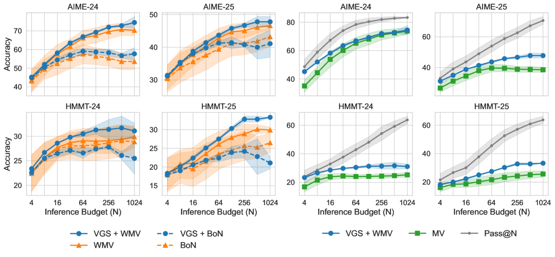
Figure 10: Per-benchmark results for Fig.˜3. (Left) Compares best-of-$N$ (BoN), weighted majority voting (WMV) and VGS with either BoN or WMV for the final aggregation. (Right) Compares VGS to majority voting (MV), a standard baseline that does not require a scorer.

C.3 Per-benchmark Plots for Fig.˜4

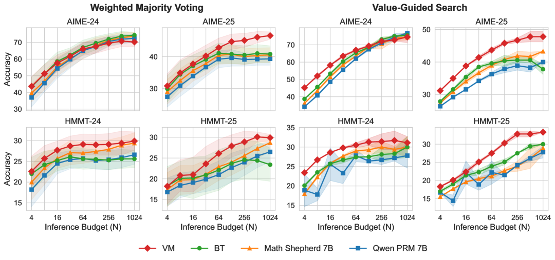
Figure 11: Per-benchmark results for Fig.˜4. Comparison of our 1.5B value model (VM), our 1.5B Bradley-Terry reward model (BT), and two 7B state-of-the-art PRMs for two TTC scaling methods: (Left) WMV or (Right) VGS (with WMV as a final aggregation step).

C.4 Per-benchmark Plots for Fig.˜5

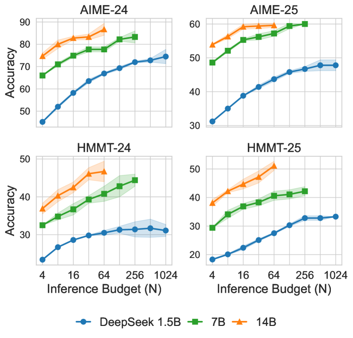
Figure 12: Per-benchmark results for Fig.˜5. With the same DeepSeek-VM-1.5B providing guidance, search continues to improve with more test-time compute.

C.5 Per-benchmark Plots for Fig.˜8

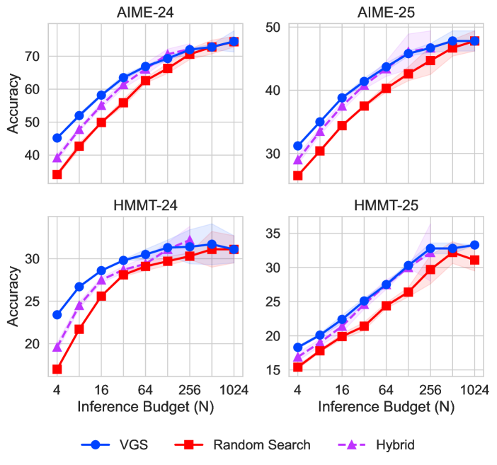
Figure 13: Per-benchmark results for Fig.˜8. Random search is the same search process as VGS except intermediate blocks are randomly selected instead of using our value model.

C.6 Results for Guiding a PPO Policy

Guo et al. [18] mentions that the performance of distilled DeepSeek models can be further enhanced through reinforcement learning (RL). In this section, we explore whether we could guide the generation of a RL trained policy. Specifically, we apply Proximal Policy Optimization (PPO) [33] to DeepSeek-1.5B using prompts from OpenR1-Cleaned and guide the trained model with DeepSeek-VM-1.5B.

We perform full parameter training with 8 H100 GPUs and use the same model as the policy for critic. We use a rule-based reward function based solely on the correctness of the response, assigning +1 for correct answers and 0 for incorrect or incomplete ones. To ensure that the learned policy $\pi$ remains close to the reference policy $\pi_{\mathrm{ref}}$, an additional KL penalty is applied to the reward:

$$r(x,y)-\gamma_{\mathrm{KL}}\left(\ln\pi(y\mid x)-\ln\pi_{\mathrm{ref}}(y\mid x)\right),$$ (1)

where $r(x,y)$ is the rule-based reward for prompt $x$ and response $y$, and $\gamma_{\mathrm{KL}}$ controls the strength of the KL penalty. To further encourage exploration, we apply standard entropy regularization by subtracting the policy entropy from the loss weighted by a coefficient $\gamma_{\mathrm{entropy}}$:

$$\mathcal{L}_{\mathrm{PPO}}-\gamma_{\mathrm{entropy}}\,\mathcal{H}[\pi(\cdot\mid x)],$$ (2)

The hyperparameter settings are shown below.

PPO Hyperparameter Setting Setting Parameters Generation (train) temperature: 1.0 top p: 1 PPO batch size: 256
mini batch size: 128
micro batch size: 1
policy learning rate: 1e-6
critic learning rate: 1e-5
train epochs: 25 $\gamma_{\mathrm{entropy}}$: 1e-3
$\gamma_{\mathrm{KL}}$: 1e-4
gae $\gamma$: 1
gae $\lambda$: 1
clip ratio: 0.2
Total number of steps: 2250

DeepSeek-1.5B	Pass@4	Pass@8	Pass@16	Pass@32	Pass@64	Pass@128	Pass@256
AIME-24	$48.7\pm 5.0$	$58.9\pm 4.9$	$67.3\pm 4.7$	$74.1\pm 3.2$	$78.4\pm 3.0$	$80.4\pm 2.4$	$81.9\pm 1.7$
AIME-25	$33.1\pm 4.1$	$39.1\pm 4.4$	$43.7\pm 3.9$	$49.0\pm 3.8$	$54.0\pm 3.9$	$58.8\pm 3.4$	$62.6\pm 3.6$
HMMT-24	$24.0\pm 4.6$	$28.6\pm 3.9$	$32.9\pm 3.6$	$37.7\pm 4.4$	$42.9\pm 4.2$	$48.1\pm 3.7$	$54.2\pm 4.9$
HMMT-25	$21.6\pm 4.6$	$26.7\pm 4.0$	$30.1\pm 4.8$	$37.8\pm 5.1$	$45.6\pm 4.6$	$52.6\pm 4.2$	$57.1\pm 3.8$
DeepSeek-1.5B-PPO	Pass@4	Pass@8	Pass@16	Pass@32	Pass@64	Pass@128	Pass@256
AIME-24	$54.0\pm 5.0$	$61.4\pm 4.6$	$67.6\pm 4.1$	$73.3\pm 3.4$	$76.8\pm 2.4$	$78.3\pm 1.7$	$79.6\pm 1.1$
AIME-25	$35.9\pm 3.9$	$39.8\pm 3.8$	$45.8\pm 4.2$	$50.9\pm 3.5$	$56.1\pm 3.0$	$59.8\pm 3.6$	$64.1\pm 3.9$
HMMT-24	$27.2\pm 4.2$	$32.8\pm 4.4$	$37.6\pm 3.6$	$41.5\pm 3.6$	$45.0\pm 3.3$	$48.8\pm 3.3$	$52.4\pm 3.4$
HMMT-25	$22.8\pm 4.0$	$26.8\pm 4.3$	$32.5\pm 4.4$	$36.9\pm 4.4$	$43.7\pm 3.8$	$48.9\pm 3.8$	$52.6\pm 3.6$

Table 3: Pass@N results for DeepSeek-1.5B model and PPO-trained DeepSeek-1.5B-PPO model.

Table˜3 presents the comparison between the DeepSeek-1.5B model and the PPO-trained model (DeepSeek-1.5B-PPO). As N increases, the performance gap gradually narrows. While the PPO-trained model performs competitively at lower $N$ values, it is surpassed by the base model at Pass@32 on both the AIME-24 and HMMT-25 datasets. This decline in performance could be attributed to the reduced entropy of the model after PPO training, which limits the diversity of model generations and negatively impacts performance at higher Pass@N.

We report our value-guided results of the PPO-trained model in Fig.˜14. We observe that VGS nicely complements PPO training and provides additional test-time compute gains in performance compared to WMV and MV.

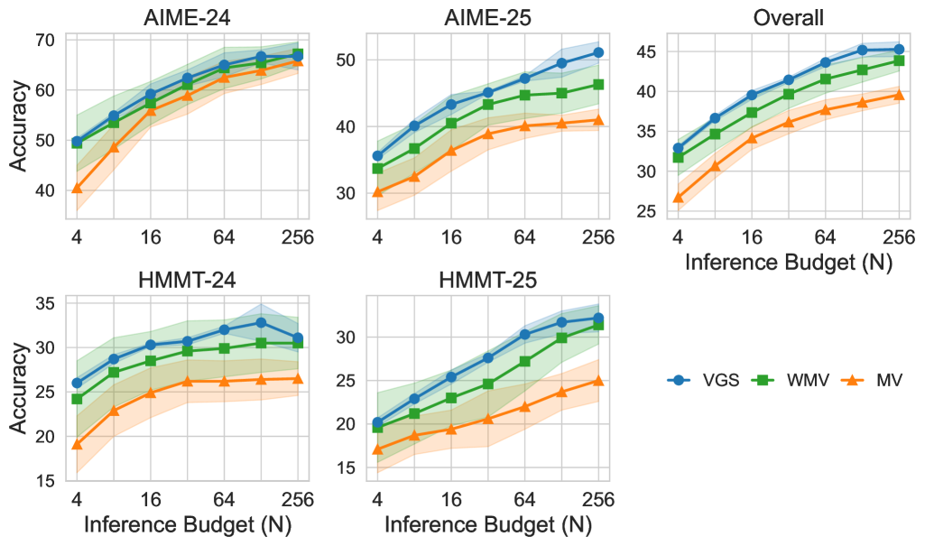
Figure 14: Guiding DeepSeek-1.5B Trained with PPO. Comparison of VGS, WMV and MV for TTC scaling our PPO policy.

C.7 Qualitative Examples

Figures 17, 18, and 19 (at the end of the paper) show representative qualitative examples where value scores from VGS are used to guide beam search. At each step, two blocks of tokens are proposed, and the one with the higher value is selected to continue the solution. Due to space constraints, parts of the beams are abridged with …, and for ease of visualization, blue highlights indicate correct reasoning steps, while red highlights denote incorrect ones.

Low-scoring beams exhibit different types of failure. In Figure 17, the rejected beam alternates between correct and incorrect steps, resulting in confused and ultimately incorrect reasoning. In Figure 18, the beam begins with a plausible strategy involving GCD analysis but eventually resorts to ineffective trial and error. In Figure 19, the beam makes a critical error in the algebraic transformation early on and fails to recover. In contrast, the selected beams across all examples demonstrate systematic reasoning and successfully solve the problems.

Interestingly, despite the critical error in Figure 19, VGS assigns a moderately high score (0.337) to the rejected beam—higher than scores for less subtle failures in earlier examples—suggesting that even significant mistakes can be difficult to detect when embedded in otherwise coherent reasoning.

Finally, we empirically compare the distribution of generation lengths between the DeepSeek-1.5B base model and VGS with DeepSeek-1.5B across all benchmarks (Figure 15). On average, VGS generates noticeably shorter responses (11,219 tokens vs. 12,793 for the DeepSeek-1.5B base model), suggesting that beam search not only enhances accuracy but also promotes more concise reasoning. This trend is consistent with our qualitative analysis, where beam search tends to favor token blocks that are direct and solution-oriented, rather than verbose or meandering reasoning. Notably, the sharp peak near 16,000 tokens corresponds to the maximum generation length of DeepSeek models (16,384). For the base model, as many as 50% of the generations reach this limit, often resulting in incomplete outputs.

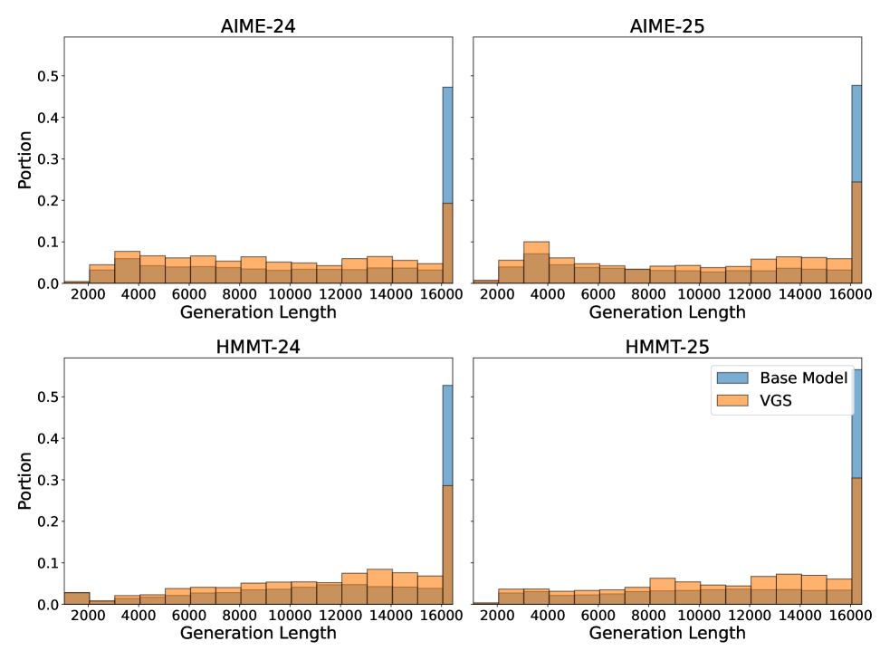
Figure 15: Histogram of generation lengths for the DeepSeek-1.5B base model vs. VGS. VGS consistently produces shorter responses across benchmarks, with average lengths of 11,219 and 12,793 tokens for VGS and the base model, respectively. The peak around 16,000 tokens reflects the generation cap of DeepSeek models, which the base model frequently hits, often resulting in incomplete outputs.

Appendix D Further Details of Data Collection

Pre-filtering process. Here we describe the pre-filtering process for constructing OpenR1-Cleaned in more detail. Below are the sequence of filtering operations we performed on OpenR1-Math [2]. We arrived at these rules by manually inspecting the data, by sampling $100$ random problems from the dataset and checking if all problems’ solutions looked reasonable to us. In OpenR1-Math, a solution is a fleshed-out solution to the math problem, an answer is the final answer to the math problem.

1. Filter out all solutions with $0$ or $>1$ boxed answers (enclosed in \boxed{}). These are ambiguous and difficult to parse out the answer.

2. Filter out answers which are difficult to automatically parse or verify. This includes answers containing: ‘or’, ‘and’ \mathrm, \quad, answers with equal signs, commas, semicolons, \cup, \cap, inequality symbols, approximation symbols.

3. Filter out multiple-choice questions, which are labeled with question_type = ‘MCQ’.

4. Filter out questions with multiple parts, as it is ambiguous which part the answer is for.

5. Filter out questions containing links (http:// or https://), since the models we test cannot access the web.

Roll-in roll-out process. We also provide further intuition for the roll-in vs. roll-out process (illustrated in Fig.˜2 left). The roll-in and then roll-out process is a standard technique in imitation learning [12] and reinforcement learning [11].

Roll-out. The roll-out process uses a fixed policy $\pi^{\text{ref}}$ to roll-out from any partial solution provided by the roll-in process. The rationale for using a fixed roll-out policy is to fix the target of the classification / value regression problem. In particular, the classifier is trained to predict the probability of each class under the roll-out policy, given the partial solution.

Roll-in. The main point of the roll-in process is to create a diverse distribution of partial solutions to roll-out from. By creating a diverse roll-in distribution with multiple roll-in policies, we can ensure that the classifier is trained on a diverse context distribution and will generalize better to new traces. To select where to cut a roll-in (to start the roll-out), we sample a cut index from the distribution of $p(i)=\frac{\sqrt{i}}{\sum_{j\in[L]}\sqrt{j}}$ where $L$ is the length of the roll-in. We chose this such that the cut index is more likely to occur at earlier positions of the roll-in. We want to encourage more learning at earlier positions since those prediction problems are more difficult than at later positions. The following figure (Fig.˜16) illustrates the distribution of the length of roll-outs, which shows that this indexing scheme indeed yields many long roll-outs.

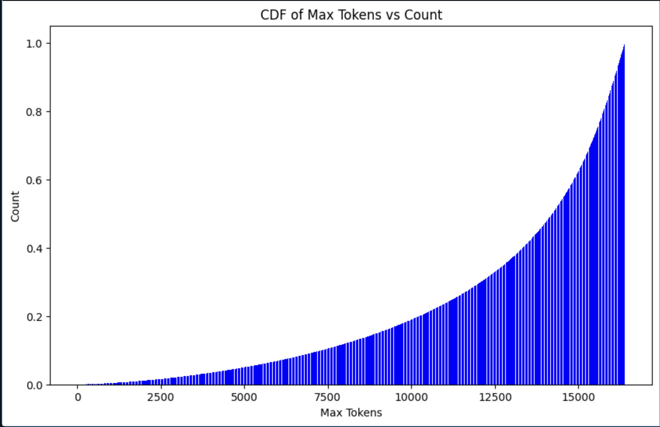
Figure 16: Distribution of roll-out length.

Appendix E Further Details for Value Model Training

Our value model DeepSeek-VM-1.5B uses the same base architecture as the DeepSeek-R1-Distill-Qwen-1.5B model, which is a 1.5B parameter transformer model with $28$ layers and $1536$ hidden size. To turn this model into a value model, we replace the LM head with a scoring head, parameterized by a two-layer MLP, that outputs logits for three classes: ‘correct’, ‘incorrect’, and ‘incomplete’. The number of classes can be modified to suit the task at hand.

Category	Parameter	Value
Model	Base Model Initialization	DeepSeek-R1-Distill-Qwen-1.5B
	Hidden size $d_{\text{model}}$	$1536$
	Score Head	two-layer MLP with hidden size $d_{\text{model}}$
	Score Head Bias	False
	Score Head Labels	$0$=Incorrect, $1$=Correct, $2$=Incomplete
Data	Dataset	OpenR1-VM
	Validation split	$500$
	Max sequence length	$16384$
Training	Batch size	$1024$
	Learning-rate schedule	Cosine with max_lr=1e-4
	Warm-up steps	$10\%$ of total steps
	Dropout	$0.05$
	Number of epochs	$5$
Optimizer	Optimizer type	AdamW
	$\beta_{1}$	$0.9$
	$\beta_{2}$	$0.95$
	Weight decay	$0.1$
	Grad Norm Clip	$5$
Compute	GPUs	$16$ nodes of $8\times\texttt{NVIDIA H100}$
	Wall-clock time (h)	24 hours
	Tokens Throughput (tokens/s)	2.07M
	Loss Tokens Throughput (loss tokens/s)	835k
	Total Tokens Processed (per epoch)	35.7B
	Total Loss Tokens Processed (per epoch)	14.4B

Table 4: Value Model Training Parameters.

We sweeped learning rates 1e-4, 3e-4, 7e-5 and we save checkpoints at every epoch. We selected the best checkpoint via WMV performance on AIME-24.

Appendix F Further Details for Inference with Search

Given a problem, the prompt we used is:

<|begin_of_sentence|><|User|>{problem} Please think step-by-step and put your final answer within \boxed{}.<|Assistant|><think>\n

We use the same decoding parameters as in the original DeepSeek paper [18].

Category	Parameter	Value
Decoding	Inference Engine	SGLang [51]
	Max generation length	$16384$
	Temperature	$0.6$
	Top-p	$0.95$
	Think Token	<think>
	End of Think Token	</think>
Best Parameters for Search (VGS)	Model	DeepSeek-VM-1.5B
	Beam width	$2$
	Block size (tokens)	$4096$
	Parallel branches (DVTS)	budget dependent
	Final aggregation rule	Weighted Majority Vote (WMV)

Table 5: Decoding and Search Parameters.

Appendix G Further Details for Training Bradley-Terry Reward Model

Dataset. Recall that our dataset for value model training (OpenR1-VM) contains $56$ responses per problem. To construct a Bradley-Terry dataset, we sample up to $4$ response pairs per problem, where a pair consists of a response with reward $0$ (the ‘reject’ response) and a response with reward $1$ (the ‘chosen’ response). Some prompts may have fewer than $4$ responses with reward $0$ or $1$, and in those cases, we include as many as possible. This yields a dataset of roughly $122$k pairs.

Model. We use the same model architecture as the value model (Appendix˜E) except that the score head outputs a single scalar score instead of a three-dimensional vector. We use the same training pipeline, except that the training loss is swapped to the standard BT loss [8]:

$$L_{\texttt{BT}}(\theta,\mathcal{B})=\frac{1}{|\mathcal{B}|}\sum_{(x,y_{r},y_{c})\in\mathcal{B}}-\log\sigma(f_{\theta}(x,y_{c})-f_{\theta}(x,y_{r})),$$ (3)

where $\sigma$ is the sigmoid function, $y_{r}$ is the reject response and $y_{c}$ is the chosen response. We use a batch size of $128$ pairs and we train for one epoch. We sweeped many learning rates: 3e-4, 1e-4, 7e-5, 3e-5, 7e-6. We found that the BT loss drops and plateaus much quicker than the value model loss, and all learning rates yielded similar final losses. We consider the last ckpt of each run and we selected lr=3e-5 as best ckpt with search (width 2, block size $4096$, WMV aggregation) on aime-24. We note that one detail for getting BT to work with weighted majority is to use the sigmoid of the BT score, i.e., take WMV with $\sigma(f_{\theta}(x,y))$ instead of $f_{\theta}(x,y)$ itself. While this doesn’t affect BoN performance, we found that taking sigmoid was crucial for WMV performance to scale well.

Appendix H Inference FLOPS Computation

In this section, we compute the FLOPs for search and show that adding value model guidance at the block-level introduces negligible compute overhead, as the vast majority of the compute is from generator model. We follow the approach outlined in Kaplan et al. [21], Sardana et al. [32] to compute the FLOPs for a single forward pass of the transformer, ignoring the embedding layers for simplicity. Consider a transformer with $n_{layer}$ layers, $d$ dimensional residual stream, $d_{ff}$ dimensional feed-forward layer, and $d$ dimensional attention outputs. Then the number of non-embedding parameters is $N=2n_{layer}d(2d+d_{ff})$, and the number of FLOPs for a single forward pass over a context of length $n_{ctx}$ is

$$C(n_{ctx})=2N+2n_{layer}n_{ctx}d.$$ (4)

Then, in the regime where $d_{model}>n_{ctx}/12$, Kaplan et al. [21], Sardana et al. [32] further approximate the above by ignoring the $n_{ctx}$ term, i.e., $C$ becomes independent of $n_{ctx}$. We adopt this approximation when estimating the inference FLOPs of our generator models. Thus, for a context length of $n_{ctx}=16,384$, the inference FLOPs for one complete generation for each generator model is $2Nn_{ctx}$:

1. DeepSeek-R1-Distill-Qwen-1.5B: $2\times 1.5B\times 16384=49.1T$.

2. DeepSeek-R1-Distill-Qwen-7B: $2\times 7B\times 16384=229T$.

3. DeepSeek-R1-Distill-Qwen-14B: $2\times 14B\times 16384=459T$.

4. DeepSeek-R1 (671B, with 37B activated params): $2\times 37B\times 16384=1212T$.

We now compute the FLOPs needed for one forward pass of the value model. Since we use a block-size of $4096$, there are at most $16384/4096=4$ value model inferences per generation. Thus, the FLOPs from the value model is:

1. 1.5B classifier: $2\times 1.5B\times 4=12B$.

2. 7B classifier (baselines): $2\times 7B\times 4=56B$.

Thus, we can see that the value model FLOPs is negligible compared to the generator model FLOPs. In particular, when guiding a 1.5B generator with a 1.5B classifier, the classifier FLOPs is only $0.024\%$ of the generator FLOPs. With a compute budget of $256$, this amounts to a total FLOPs of $(49.1T+12B)\times 256=12.6P$. When guiding with a 7B classifier, the total FLOPs is $(49.1T+56B)\times 256=12.6P$. Note that the FLOPs required for generating $256$ independent generations is $49.1T\times 256=12.6P$. Thus, search has a negligible overhead comapred to (weighted) majority voting or best of $n$.

Figure 17: Example of selected and rejected beams during beam search with VGS. The high-scoring beam (score 0.996) follows a correct and coherent line of reasoning, arriving at the correct answer. In contrast, the rejected beam (score 0.009) contains several inconsistencies and incorrect steps, despite occasionally making correct logical deduction—demonstrating the effectiveness of VGS as a value model. Highlighting is added for clarity: blue indicates correct reasoning steps or results, while red indicates incorrect ones. Part of generations are abridged with $\ldots$ notation.

Figure 18: Additional examples of selected and rejected beams under VGS. The high-scoring beam applies a concise and effective modular reasoning strategy whereas the rejected beam attempts several approaches—including an incorrect use of the Factor Theorem and trial-and-error—but ultimately fails. Color coding follows Figure 17. Part of generations are abridged with $\ldots$ notation.

Figure 19: Additional examples of selected and rejected beams under VGS. The rejected beam misrepresents Derek’s transformation, leading to an incorrect equation that derails the solution. In contrast, the high-scoring beam correctly models the relationship and systematically solves for the unique valid value of $a$. Color coding follows Figure 17. Part of generations are abridged with $\ldots$ notation.

References

- Abdin et al. [2025] Marah Abdin, Sahaj Agarwal, Ahmed Awadallah, Vidhisha Balachandran, Harkirat Behl, Lingjiao Chen, Gustavo de Rosa, Suriya Gunasekar, Mojan Javaheripi, Neel Joshi, et al. Phi-4-reasoning technical report. arXiv preprint arXiv:2504.21318, 2025.
- Allal et al. [2025] Loubna Ben Allal, Lewis Tunstall, Anton Lozhkov, Elie Bakouch, Guilherme Penedo, Hynek Kydlicek, and Gabriel Martín Blázquez. Open r1: Update #2. https://huggingface.co/blog/open-r1/update-2, February 2025. Hugging Face Blog.
- Ayoub et al. [2024] Alex Ayoub, Kaiwen Wang, Vincent Liu, Samuel Robertson, James McInerney, Dawen Liang, Nathan Kallus, and Csaba Szepesvári. Switching the loss reduces the cost in batch (offline) reinforcement learning. arXiv preprint arXiv:2403.05385, 2024.
- Bai et al. [2022] Yuntao Bai, Saurav Kadavath, Sandipan Kundu, Amanda Askell, Jackson Kernion, Andy Jones, Anna Chen, Anna Goldie, Azalia Mirhoseini, Cameron McKinnon, et al. Constitutional ai: Harmlessness from ai feedback. arXiv preprint arXiv:2212.08073, 2022.
- Batra et al. [2012] Dhruv Batra, Payman Yadollahpour, Abner Guzman-Rivera, and Gregory Shakhnarovich. Diverse m-best solutions in markov random fields. In Computer Vision–ECCV 2012: 12th European Conference on Computer Vision, Florence, Italy, October 7-13, 2012, Proceedings, Part V 12, pages 1–16. Springer, 2012.
- Beeching et al. [2024] Edward Beeching, Lewis Tunstall, and Sasha Rush. Scaling test-time compute with open models, 2024. URL https://huggingface.co/spaces/HuggingFaceH4/blogpost-scaling-test-time-compute.
- Bellemare et al. [2017] Marc G Bellemare, Will Dabney, and Rémi Munos. A distributional perspective on reinforcement learning. In International conference on machine learning, pages 449–458. PMLR, 2017.
- Bradley and Terry [1952] Ralph Allan Bradley and Milton E Terry. Rank analysis of incomplete block designs: I. the method of paired comparisons. Biometrika, 39(3/4):324–345, 1952.
- Brown et al. [2024] Bradley Brown, Jordan Juravsky, Ryan Ehrlich, Ronald Clark, Quoc V Le, Christopher Ré, and Azalia Mirhoseini. Large language monkeys: Scaling inference compute with repeated sampling. arXiv preprint arXiv:2407.21787, 2024.
- Burns et al. [2023] Collin Burns, Pavel Izmailov, Jan Hendrik Kirchner, Bowen Baker, Leo Gao, Leopold Aschenbrenner, Yining Chen, Adrien Ecoffet, Manas Joglekar, Jan Leike, et al. Weak-to-strong generalization: Eliciting strong capabilities with weak supervision. arXiv preprint arXiv:2312.09390, 2023.
- Chang et al. [2023] Jonathan D Chang, Kiante Brantley, Rajkumar Ramamurthy, Dipendra Misra, and Wen Sun. Learning to generate better than your llm. arXiv preprint arXiv:2306.11816, 2023.
- Chang et al. [2015] Kai-Wei Chang, Akshay Krishnamurthy, Alekh Agarwal, Hal Daumé III, and John Langford. Learning to search better than your teacher. In International Conference on Machine Learning, pages 2058–2066. PMLR, 2015.
- Chen et al. [2024] Guoxin Chen, Minpeng Liao, Chengxi Li, and Kai Fan. Alphamath almost zero: Process supervision without process. In The Thirty-eighth Annual Conference on Neural Information Processing Systems, 2024. URL https://openreview.net/forum?id=VaXnxQ3UKo.
- Cobbe et al. [2021] Karl Cobbe, Vineet Kosaraju, Mohammad Bavarian, Mark Chen, Heewoo Jun, Lukasz Kaiser, Matthias Plappert, Jerry Tworek, Jacob Hilton, Reiichiro Nakano, et al. Training verifiers to solve math word problems. arXiv preprint arXiv:2110.14168, 2021.
- Davies et al. [1998] Scott Davies, Andrew Y Ng, and Andrew Moore. Applying online search techniques to continuous-state reinforcement learning. In AAAI/IAAI, pages 753–760, 1998.
- El-Kishky et al. [2025] Ahmed El-Kishky, Alexander Wei, Andre Saraiva, Borys Minaiev, Daniel Selsam, David Dohan, Francis Song, Hunter Lightman, Ignasi Clavera, Jakub Pachocki, et al. Competitive programming with large reasoning models. arXiv preprint arXiv:2502.06807, 2025.
- Farebrother et al. [2024] Jesse Farebrother, Jordi Orbay, Quan Vuong, Adrien Ali Taïga, Yevgen Chebotar, Ted Xiao, Alex Irpan, Sergey Levine, Pablo Samuel Castro, Aleksandra Faust, et al. Stop regressing: Training value functions via classification for scalable deep rl. arXiv preprint arXiv:2403.03950, 2024.
- Guo et al. [2025] Daya Guo, Dejian Yang, Haowei Zhang, Junxiao Song, Ruoyu Zhang, Runxin Xu, Qihao Zhu, Shirong Ma, Peiyi Wang, Xiao Bi, and Others. Deepseek-r1: Incentivizing reasoning capability in llms via reinforcement learning. arXiv preprint arXiv:2501.12948, 2025.
- Han et al. [2024] Seungwook Han, Idan Shenfeld, Akash Srivastava, Yoon Kim, and Pulkit Agrawal. Value augmented sampling for language model alignment and personalization. arXiv preprint arXiv:2405.06639, 2024.
- Imani et al. [2024] Ehsan Imani, Kai Luedemann, Sam Scholnick-Hughes, Esraa Elelimy, and Martha White. Investigating the histogram loss in regression. arXiv preprint arXiv:2402.13425, 2024.
- Kaplan et al. [2020] Jared Kaplan, Sam McCandlish, Tom Henighan, Tom B Brown, Benjamin Chess, Rewon Child, Scott Gray, Alec Radford, Jeffrey Wu, and Dario Amodei. Scaling laws for neural language models. arXiv preprint arXiv:2001.08361, 2020.
- Kydl´ıček [2025] Hynek Kydlíček. Math-verify: Math verification library, 2025. URL https://github.com/huggingface/Math-Verify. A library to rule-based verify mathematical answers.
- Lightman et al. [2023] Hunter Lightman, Vineet Kosaraju, Yuri Burda, Harrison Edwards, Bowen Baker, Teddy Lee, Jan Leike, John Schulman, Ilya Sutskever, and Karl Cobbe. Let’s verify step by step. In The Twelfth International Conference on Learning Representations, 2023.
- Liu et al. [2023] Jiacheng Liu, Andrew Cohen, Ramakanth Pasunuru, Yejin Choi, Hannaneh Hajishirzi, and Asli Celikyilmaz. Don’t throw away your value model! generating more preferable text with value-guided monte-carlo tree search decoding. arXiv preprint arXiv:2309.15028, 2023.
- Liu et al. [2025] Runze Liu, Junqi Gao, Jian Zhao, Kaiyan Zhang, Xiu Li, Biqing Qi, Wanli Ouyang, and Bowen Zhou. Can 1b llm surpass 405b llm? rethinking compute-optimal test-time scaling. arXiv preprint arXiv:2502.06703, 2025.
- Lowerre [1976] Bruce T Lowerre. The harpy speech recognition system. Carnegie Mellon University, 1976.
- Luo et al. [2024] Liangchen Luo, Yinxiao Liu, Rosanne Liu, Samrat Phatale, Meiqi Guo, Harsh Lara, Yunxuan Li, Lei Shu, Yun Zhu, Lei Meng, et al. Improve mathematical reasoning in language models by automated process supervision. arXiv preprint arXiv:2406.06592, 2024.
- Mudgal et al. [2023] Sidharth Mudgal, Jong Lee, Harish Ganapathy, YaGuang Li, Tao Wang, Yanping Huang, Zhifeng Chen, Heng-Tze Cheng, Michael Collins, Trevor Strohman, et al. Controlled decoding from language models. arXiv preprint arXiv:2310.17022, 2023.
- Muennighoff et al. [2025] Niklas Muennighoff, Zitong Yang, Weijia Shi, Xiang Lisa Li, Li Fei-Fei, Hannaneh Hajishirzi, Luke Zettlemoyer, Percy Liang, Emmanuel Candès, and Tatsunori Hashimoto. s1: Simple test-time scaling. arXiv preprint arXiv:2501.19393, 2025.
- Petrov et al. [2025] Ivo Petrov, Jasper Dekoninck, Lyuben Baltadzhiev, Maria Drencheva, Kristian Minchev, Mislav Balunović, Nikola Jovanović, and Martin Vechev. Proof or bluff? evaluating llms on 2025 usa math olympiad. arXiv preprint arXiv:2503.21934, 2025.
- Qwen Team [2025] Qwen Team. Qwen3: Think deeper, act faster, 2025. URL https://qwenlm.github.io/blog/qwen3/. Accessed: 2025-05-08.
- Sardana et al. [2023] Nikhil Sardana, Jacob Portes, Sasha Doubov, and Jonathan Frankle. Beyond chinchilla-optimal: Accounting for inference in language model scaling laws. arXiv preprint arXiv:2401.00448, 2023.
- Schulman et al. [2017] John Schulman, Filip Wolski, Prafulla Dhariwal, Alec Radford, and Oleg Klimov. Proximal policy optimization algorithms, 2017. URL https://arxiv.org/abs/1707.06347.
- Setlur et al. [2025] Amrith Setlur, Chirag Nagpal, Adam Fisch, Xinyang Geng, Jacob Eisenstein, Rishabh Agarwal, Alekh Agarwal, Jonathan Berant, and Aviral Kumar. Rewarding progress: Scaling automated process verifiers for LLM reasoning. In The Thirteenth International Conference on Learning Representations, 2025. URL https://openreview.net/forum?id=A6Y7AqlzLW.
- Silver et al. [2017] David Silver, Thomas Hubert, Julian Schrittwieser, Ioannis Antonoglou, Matthew Lai, Arthur Guez, Marc Lanctot, Laurent Sifre, Dharshan Kumaran, Thore Graepel, et al. Mastering chess and shogi by self-play with a general reinforcement learning algorithm. arXiv preprint arXiv:1712.01815, 2017.
- Snell et al. [2025] Charlie Victor Snell, Jaehoon Lee, Kelvin Xu, and Aviral Kumar. Scaling LLM test-time compute optimally can be more effective than scaling parameters for reasoning. In The Thirteenth International Conference on Learning Representations, 2025. URL https://openreview.net/forum?id=4FWAwZtd2n.
- Starace et al. [2025] Giulio Starace, Oliver Jaffe, Dane Sherburn, James Aung, Jun Shern Chan, Leon Maksin, Rachel Dias, Evan Mays, Benjamin Kinsella, Wyatt Thompson, et al. Paperbench: Evaluating ai’s ability to replicate ai research. arXiv preprint arXiv:2504.01848, 2025.
- Sun et al. [2024] Jiashuo Sun, Yi Luo, Yeyun Gong, Chen Lin, Yelong Shen, Jian Guo, and Nan Duan. Enhancing chain-of-thoughts prompting with iterative bootstrapping in large language models. In Kevin Duh, Helena Gomez, and Steven Bethard, editors, Findings of the Association for Computational Linguistics: NAACL 2024, pages 4074–4101, Mexico City, Mexico, June 2024. Association for Computational Linguistics. doi: 10.18653/v1/2024.findings-naacl.257. URL https://aclanthology.org/2024.findings-naacl.257/.
- Sutton et al. [1998] Richard S Sutton, Andrew G Barto, et al. Reinforcement learning: An introduction, volume 1. MIT press Cambridge, 1998.
- Vijayakumar et al. [2016] Ashwin K Vijayakumar, Michael Cogswell, Ramprasath R Selvaraju, Qing Sun, Stefan Lee, David Crandall, and Dhruv Batra. Diverse beam search: Decoding diverse solutions from neural sequence models. arXiv preprint arXiv:1610.02424, 2016.
- Wang et al. [2025a] Junlin Wang, Shang Zhu, Jon Saad-Falcon, Ben Athiwaratkun, Qingyang Wu, Jue Wang, Shuaiwen Leon Song, Ce Zhang, Bhuwan Dhingra, and James Zou. Think deep, think fast: Investigating efficiency of verifier-free inference-time-scaling methods. arXiv preprint arXiv:2504.14047, 2025a.
- Wang et al. [2023a] Kaiwen Wang, Kevin Zhou, Runzhe Wu, Nathan Kallus, and Wen Sun. The benefits of being distributional: Small-loss bounds for reinforcement learning. Advances in neural information processing systems, 36:2275–2312, 2023a.
- Wang et al. [2025b] Kaiwen Wang, Nathan Kallus, and Wen Sun. The central role of the loss function in reinforcement learning. Statistical Science, 2025b. Forthcoming.
- Wang et al. [2023b] Peiyi Wang, Lei Li, Zhihong Shao, RX Xu, Damai Dai, Yifei Li, Deli Chen, Yu Wu, and Zhifang Sui. Math-shepherd: Verify and reinforce llms step-by-step without human annotations. arXiv preprint arXiv:2312.08935, 2023b.
- Wang et al. [2022] Xuezhi Wang, Jason Wei, Dale Schuurmans, Quoc Le, Ed Chi, Sharan Narang, Aakanksha Chowdhery, and Denny Zhou. Self-consistency improves chain of thought reasoning in language models. arXiv preprint arXiv:2203.11171, 2022.
- Wang et al. [2023c] Xuezhi Wang, Jason Wei, Dale Schuurmans, Quoc V Le, Ed H. Chi, Sharan Narang, Aakanksha Chowdhery, and Denny Zhou. Self-consistency improves chain of thought reasoning in language models. In The Eleventh International Conference on Learning Representations, 2023c. URL https://openreview.net/forum?id=1PL1NIMMrw.
- Yao et al. [2023] Shunyu Yao, Dian Yu, Jeffrey Zhao, Izhak Shafran, Tom Griffiths, Yuan Cao, and Karthik Narasimhan. Tree of thoughts: Deliberate problem solving with large language models. Advances in neural information processing systems, 36:11809–11822, 2023.
- Zhang et al. [2024a] Di Zhang, Xiaoshui Huang, Dongzhan Zhou, Yuqiang Li, and Wanli Ouyang. Accessing gpt-4 level mathematical olympiad solutions via monte carlo tree self-refine with llama-3 8b. arXiv preprint arXiv:2406.07394, 2024a.
- Zhang et al. [2024b] Hanning Zhang, Pengcheng Wang, Shizhe Diao, Yong Lin, Rui Pan, Hanze Dong, Dylan Zhang, Pavlo Molchanov, and Tong Zhang. Entropy-regularized process reward model. arXiv preprint arXiv:2412.11006, 2024b.
- Zhang et al. [2025] Zhenru Zhang, Chujie Zheng, Yangzhen Wu, Beichen Zhang, Runji Lin, Bowen Yu, Dayiheng Liu, Jingren Zhou, and Junyang Lin. The lessons of developing process reward models in mathematical reasoning. arXiv preprint arXiv:2501.07301, 2025.
- Zheng et al. [2024] Lianmin Zheng, Liangsheng Yin, Zhiqiang Xie, Chuyue Livia Sun, Jeff Huang, Cody Hao Yu, Shiyi Cao, Christos Kozyrakis, Ion Stoica, Joseph E Gonzalez, et al. Sglang: Efficient execution of structured language model programs. Advances in Neural Information Processing Systems, 37:62557–62583, 2024.
- Zhou et al. [2025] Jin Peng Zhou, Kaiwen Wang, Jonathan Chang, Zhaolin Gao, Nathan Kallus, Kilian Q Weinberger, Kianté Brantley, and Wen Sun. : Provably optimal distributional rl for llm post-training. arXiv preprint arXiv:2502.20548, 2025.