FRIREN: Beyond Trajectories — A Spectral Lens on Time

Abstract

Long-Term Time-Series Forecasting (LTSF) models often position themselves as general-purpose solutions ready to be deployed in different fields, implicitly assuming any data is pointwise predictable. Using chaotic systems like Lorenz-63 as a touchstone, we argue that geometry—not pointwise predictions—is the appropriate abstraction level for a truly dynamic-agnostic foundational model. Minimizing Wasserstein-2 distance (W2), a metric that measures geometric changes, and exposing a clear spectral view of dynamics, are key for long horizon forecasting. Our model FRIREN (Flow-inspired Representations via Interpretable Eigen-networks), implements an Augmented Normalizing-Flow block that embeds data into a normally distributed latent representation. It then produces a W2-efficient optimal path, decomposable as "rotate, stretch, rotate back, and translate". This design yields (i) locally generated, geometric structure preserving predictions that bypass underlying dynamics, and (ii) a global spectral representation that doubles as a finite Koopman operator when slightly modified, letting practitioners inspect which modes grow, damp, or oscillate across at both local and system levels. FRIREN achieves an MSE of 11.4, MAE of 1.6, and SWD of 0.96 on Lorenz-63 in a 336-in-336-out, dt=0.01 setting, decisively surpassing TimeMixer (MSE 27.3, MAE 2.8, SWD 2.1). Our model maintains effective prediction for 274 out of 336 steps, nearly 2.5 Lyapunov times. On Rossler (96-in, 336-out), FRIREN achieves an MSE 0.0349, MAE 0.0953, and SWD 0.0170, outperforming TimeMixer‘s MSE 4.3988, MAE 0.886, and SWD 3.2065. It remains competitive on standard LTSF datasets such as ETT and Weather. FRIREN bridges the gap between modern generative flows and classical spectral analysis, making long-term forecasting both accurate and interpretable—setting a new standard for LTSF model design.

1 Introduction

Deep learning models, including transformers, linear methods, and LLMs (Wu et al., 2022; Zhou et al., 2021; Zeng et al., 2023; Nie et al., 2022; Wang et al., 2024; Das et al., 2024), are now standard for Long-Term Time Series Forecasting (LTSF). The community largely treats them as dynamics-agnostic tools, implicitly assuming that complex patterns are simply pointwise predictable in a data-driven way—even under a simultaneous mix of stochastic, chaotic and non-stationary influences. This demand for robustness is justified, as mixtures of these dynamics are ubiquitous in real-world systems, from climate and power grids to finance. Even standard LTSF benchmarks like the ETT dataset (Zhou et al., 2021) exhibits known chaotic characteristics ((Hu et al., 2024), Section E.2). However, a strong solution in a very general setting cannot just be assumed to exist thanks to the successful transformer architecture Vaswani et al. (2017) without careful analysis of the predictability of datasets. In sharp critiques, Bergmeir (2023) questions benchmarking on nearly random-walk dataset (Exchange Rate), and Zeng et al. (2023) demonstrated transformer modules alone, without the widely acknowledged technique such as patching and smoothing, offer limited accuracy improvement against a simple linear model (DLinear) where one regression predicts the smoothed trend and another predicts the residual.

This paper challenges the dynamics-agnostic assumption with a canonical problem: Can you predict the butterfly? This refers to the 1963 Lorenz system (Lorenz, 1963) (Figure˜3 for visualization and Section˜A.2.1 for governing equations), whose butterfly-shaped attractor (a set of states that a system evolves towards) is the emblem of the "butterfly effect". As a purely deterministic process, its defining property is a sensitive dependence on initial conditions: “any two points that lie arbitrarily close to each other will move apart so dramatically that it is impossible to verify, after a reasonably short period, whether they were ever close to each other” (Osinga, 2018). Even if the governing equations were known and initial conditions measured near perfectly (both are very hard to reverse engineer), any infinitesimally small errors in measurement still grow exponentially, rendering long-term trajectory forecasting impossible, even in such ideal situations. For purely data-driven autoregressive models, the challenge is even greater: the system’s non-repeating, non-crossing trajectories make learned stepwise patterns misleading, causing prediction errors to compound catastrophically.

Amid this chaos, the hidden order is the system’s geometry. Takens’ Embedding Theorem (Takens, 1981) provides a remarkable guarantee: a time-delay embedding of a single variable can reconstruct a diffeomorphism of the system’s full attractor, preserving its topological structure (see Theorem˜A.1). A diffeomorphic transformation is a smooth and invertible transformation; intuitively, it means the butterfly-shaped attractor is bent or stretched, but not glued and torn. This stable, predictable geometric object captures the complete distribution of possible system states. Thus, the answer to our question is: “No, you cannot predict the exact trajectory. However, if you can reconstruct the attractor, you can place your prediction on it, and the range of error will be well-controlled." Thus, our core claim: predict geometry, not trajectory.

In the Lorenz system, the difficulty arises from the mesmerizing dance of particles between ‘wings’: they swirl within one lobe before irregularly switching to the other. Therefore, asking LTSF models if they can predict the next 96, 196, 336, and 720 steps ahead, where each step advances the system by 0.01 model time units (MTU), is a crucial stress test. Our results in LABEL:app:tab:lorenz63 are stark: on a short-term (96-step) forecast, DLinear—a strong benchmark performer on ETT—has 50$\times$ higher error than our model, FRIREN, and 20$\times$ higher than PatchTST and TimeMixer. This demonstrates that models optimized for stochastic trends can fail dramatically on deterministic chaos.

Forecasting is a trade-off between task strength and structural generality. Enhanced with governing equation discovery techniques (e.g. Brunton et al. (2016b) and Conti et al. (2024)), even autoregressive model exclusively designed for chaotic system can achieve a remarkable stability (Wang and Li, 2024). A truly general model, however, must be robust to different sources of unpredictability: (1) stochasticity, (2) deterministic chaos, and (3) external non-stationary shocks. We propose that the most robust abstraction level for such foundational model is pattern matching via geometry. Our model, FRIREN, embodies the principle of geometric conservatism: it aims to identify and preserve the stable geometric structures that represent conserved mechanisms amidst noise and chaos. By focusing on learning geometry-preserving maps, it excels where trajectory-based models fail, offering a new path toward building more robust and interpretable forecasting systems.

2 Method: Geometric Prediction via Location-Scale Optimal Transport

Beyond Pointwise Accuracy: Distributional Fidelity

Concretely, how to quantify the geometric closeness or distributional fidelity between prediction and real target data? For intuition, consider the two examples:

Example 1: You ask two oracles about the temperature in the next 24 hours. The first gives you an accurate hourly forecast, but each prediction is ahead by exactly three hours; the second only returns a 24-hour average for inquiries about any specific hour. Example 2: The sequences $[0,1,2,3,4]$ and $[1,2,3,4,5]$ are “similar” as a positional translation. The MSE is 1. However, $[0,2,4,6,8]$ and $[2,4,6,8,10]$ convey roughly the same degree of “similarity”, but with a MSE of 4.

Recall that in LTSF, the task is a direct multi-step prediction where past values in a time-delayed embeddings $x_{1},\dots,x_{n}$ map to future values $y\_1,\dots,y\_k$ (with $x_{n+1}\coloneqq y_{1}$), typically over horizons of 96, 196, 336, or 720. Mean squared error (MSE), defined as $\mathbb{E}_{x}[\mathbb{E}_{y\sim P(y|x)}[\|y_{pred}(x)-y_{real}\|^{2}]]$, thus measures only the average performance, ignoring the superior distributional fidelity of the first oracle’s prediction and failing to capture the intuitive similarity in the second example. The key element lost in MSE is invariance to phase shifts.

A metric that better captures the shape and is almost invariant to such shifts is the Wasserstein-2 distance Wasserstein-2 distance (W2) (see Section˜A.7 for definition, and refer to (Lei et al., 2017) for visualizations). It measures the minimal quadratic Euclidean/L2 costs required to transform one distribution into the other. Since the metric penalizes unnecessary distortions, distributional fidelity is preserved. W2 is deeply connected to optimal transport theory and in fact, the word optimal suggests the path incurs the lowest W2 among all. (Villani, 2008)

Unfortunately, W2 is computationally expensive. We approximate it by the computationally efficient Sliced Wasserstein-2 distance (SWD) (Rabin et al., 2012). Empirically, however, MSE and SWD exhibit a trade-off near the optimization boundary, where improving one often degrades the other (we will discuss this phenomenon in detail). When MSE or its variant Huber loss (it becomes MSE when the target is close, and L1 when the target is far off) is still the dominating paradigm, can we nevertheless design a geometrically conservative prediction model? A model that simultaneously balances both average performance and distributional similarity?

Fundamentally, geometric conservatism is about the worst behaviour of each particle beyond finding a conditional mean: no wasteful movement is allowed. We can exploit the connection between W2 and optimal paths: we find an intermediate representation $\mu_{z}(\tilde{y})$ as a “middleman”, and it must be close to $y_{real}$ and $y_{pred}$ in W2 sense.

$$W_{2}(p(y_{pred}|x),p(y_{real}|x))\leq\underbrace{W_{2}(p(y_{real}|x),\mu_{z}(\tilde{y}))}_{\text{(I) Center Accuracy}}+\underbrace{W_{2}(\mu_{z}(\tilde{y}),p(y_{pred}|x))}_{\text{(II) Unfold Effort}}$$ (1)

Part I simply says $\mu_{z}(\tilde{y})$ itself must be distributionally similar to the target data, and Part II says “unfolding” from $\mu_{z}(\tilde{y})$ into final prediction $y_{pred}$ must be efficient. Since an optimal path is by definition the most efficient path to (the induced measure of) $y_{pred}$, when we deliberately use a transformation from the optimal path class, the part II “leg” of the triangle is “tight”, meaning no other class of model can reach the same prediction with less effort or lower W2. Once we do our best to lower W2 in part I, we end up with a prediction bounded in W2.

Here is the most common scenario: a deterministic model trying to match the conditional expectation of the predictor $Q=\mathbb{P}(y_{pred}|x)$ to that of data $P=\mathbb{P}(y_{real}|x)$. As a deterministic model trained under MSE, the output as a point estimate $Q=\delta_{y_{pred}}\approx\mathbb{E}[P]$ is a Dirac mass. It turns out that for deterministic point estimates, minimizing W2 is equivalent to minimizing MSE, and that is all one can do to lower W2.

Proposition 2.1 (Square Factorization).

The squared Wasserstein-2 distance between the predicted and target distributions decomposes exactly:

$$W_{2}^{2}(Q,P)=\underbrace{\|\mathbb{E}[Q]-\mathbb{E}[P]\|^{2}}_{\text{(I) Location Error}}\;+\;\underbrace{W_{2}^{2}(Q_{\mathrm{centered}},P_{\mathrm{centered}})}_{\text{(II) Shape Fidelity}}$$ (2)

where $Q_{\mathrm{centered}}=Q-\mathbb{E}[Q]$. Square factorization splits W2 cleanly into decoupled subtasks: The first term Location Error term $\|\mathbb{E}[Q]-\mathbb{E}[P]\|^{2}$ precisely matches MSE minimization objective: conditional mean matching between prediction and target. The second term Shape Fidelity $W_{2}^{2}(Q_{\text{centered}},P_{\text{centered}})$ captures residual shape mismatching. For a deterministic translation vector $t$, since $(Q+t)_{\mathrm{centered}}=(Q+t)-\mathbb{E}[Q+t]=(Q-\mathbb{E}[Q])=Q_{\mathrm{centered}}$, $t$ does not affect shape fidelity. This implies to reduce W2, our model must both predict the correct average and retain sufficient stochastic spread to minimize shape error. Otherwise, for a Dirac mass $Q$, the second term approximates the variance of target, and it is not reducible. Note that identity illustrates the components of W2 but has nothing to do with training objective—in fact, training objective other than MSE that can drive MSE lower is helping with W2 minimization.

Model Architecture

We therefore need to inject a minimum level randomness into $Q$ to keep it from degenerating into a Dirac mass. We introduce a data-dependent latent variable $z\sim N(\mu(x),\sigma(x))$ into our predictor. and $Q(\cdot|x,z)$ now retains genuine spread, and varying z yields a family of conditional means $\mathbb{E}_{x}\!\bigl{[}Q(x,z)\bigr{]}$. We also should take advantage of the decoupled separation of concerns implied by square factorization: let $y_{0}$ be an anchor point, which can be generated from $z$ (as a distribution) or $x$ (as a deterministic point estimate). A shift t(z) translates the distribution, and A(z) does the scaling part. We leave the details of $A(z)$ for later. Formally,

$$OT(y_{0})=y_{0}\xmapsto{A(z)}A(z)y_{0}\xmapsto{+\,t(z)}y_{\mathrm{pred}}\quad\text{,}\quad\nabla_{y_{0}}OT(y_{0})=A(z),\;A(z)=A(z)^{\top},\;A(z)\succeq 0$$

Here the center distributions $\mu_{z}(\tilde{y})\coloneqq y_{0}+t(z)$ function as a “middleman”.

Model Implementation via Augmented Normalizing Flows

Our task is to implement $z$, $A(\cdot)$ and $t(\cdot)$. A highly expressive and flexible candidate is the Augmented Normalizing Flow block popularized by Huang et al. (2020). Each block contains several scale-and-translate layers (affine coupling layers or ACL), which is as simple as $[x_{1},x_{2}]\to[2x_{1}-3,3x_{2}+1]$. Formally, an ACL transformation of $x$ based on $z$ is $ACL(x;z)=\mathbf{s}(\mathbf{z})\odot\mathbf{x}+\mathbf{t}(\mathbf{z})$, i.e. parameters used to transformed one component are generated from the other component. Given data $x$ and normally distributed augment $z$, the block alternates between modifying the augment based on data and vice versa, creating the chained structure $x\to{z_{1}}\to x\to z_{2}...$ (using newly drawn $z_{1}$, $z_{2}$ empirically provides better stability). Given enough capacity, the paper proved that it can transform between two arbitrary continuous distributions (such as a cat picture and a multivariate normal distribution) on $\mathbb{R}^{m}$ smoothly and invertibly using only scaling and translating. Figure˜1 provides a simple illustration of data-dependency for audiences not familiar with the Normalizing Flow literature.

Figure 1: Mechanism of the affine coupling layers (ACL).

EigenACL: Data-Dependent Rotations for Interpretability

We adapt the structure for prediction by maintaining the chained $x\to{z}\to x\to z...$ embedding process but modifying the final layer to map $z\to y_{0}\in\mathbb{R}^{n}$ instead of back to $x$. The earlier layers encode the input data into a refined Gaussian latent representation $z\sim\mathcal{N}(\mu_{\phi},\sigma_{\phi}^{2})\in\mathbb{R}^{h}$while the final layer decodes this into an anchor point $y_{0}\in\mathbb{R}^{n}$ that undergoes further scale and translation transformations based on $z$.

ACLs are powerful and elegant but lack interpretability. Consider $y_{1}:=x_{51}=1.75\cdot x_{1}+2$ and $y_{2}:=x_{52}=1.9\cdot x_{2}+2.4$. Why multiply $x_{1}$ by 1.75 but $x_{2}$ by 1.9? Despite its simple appearance, this remains a linearized black box.

We propose EigenACL for interpretability: in the final layer, a data-driven orthogonal matrix serves as eigenvectors, with scaling coefficients as eigenvalues. Formally: $\mathbf{H}(\mathbf{z})\mathbf{S(z)}\mathbf{H}^{\top}(\mathbf{z})+\mathbf{t(z)}$. This introduces a third linear operation beyond scaling and translation. When eigenvalues like 1.75 and 1.9 pair with inspectable modes, they reveal crucial insights: which directions are growing or decaying, and their relative importance.

Data-dependent rotations can be implemented efficiently, requiring only matrix-vector products. A Householder reflection is a matrix $\mathbf{H_{i}}=\mathbf{I}-2\mathbf{v_{i}}\mathbf{v_{i}}^{T}$, where $\mathbf{v_{i}}$ is a unit normal vector generated from $\psi(z)$ with $\psi$ being a neural network. Each $\mathbf{H_{i}}$ is symmetric and has determinant $-1$, geometrically reflecting vectors across the hyperplane defined by normal $\mathbf{v_{i}}$.

When composing an even number of these reflections, $\mathbf{H}=\mathbf{H}_{n}\cdots\mathbf{H}_{2}\mathbf{H}_{1}$, we obtain an orthogonal matrix $\mathbf{H}$ with determinant $+1$ (a proper rotation). Inverting this transformation requires only transposition: $\mathbf{H}^{T}=(\mathbf{H}_{n}\cdots\mathbf{H}_{2}\mathbf{H}_{1})^{T}=\mathbf{H}_{1}\mathbf{H}_{2}\cdots\mathbf{H}_{n}$, making both forward and inverse transformations computationally efficient.

Geometrically, EigenACL transforms “scale, then translate” into “rotate, scale, rotate back, then translate.” Instead of scaling each time-delayed embedding coordinate independently, we rotate to a data-driven coordinate system aligned with the system’s natural modes, scale their importance, and then rotate back before translation. Since any $n$-dimensional rotation decomposes into $n$ Householder matrix products, a product of $n$ such matrices implies a thorough search of all possible rotations. In practice, the number of Householder matrices is far less than the dimensions, this creates a low-rank approximation of the optimal data-driven orthogonal directions. Another intuition is that scaling effectively acted as elementwise activation functions in plain ACL. EigenACL effectively converts it into more expressive matrix-valued activation functions.

Why is EigenACL an Optimal Path

The Brenier Theorem (Brenier, 1991) (McCann, 1995) (see Theorem˜A.2 for full details) tells us that when transportation cost is quadratic Euclidean and the source distribution is absolutely continuous, there exists a unique cost-minimizing map (the optimal path) from the source measure $\mu_{z}$ to the target measure $y_{pred}$ induced by the map. This map itself is also the gradient of some convex potential function. This is the key reason that we only use W2 (whose cost function is quadratic L2) and that we insist using a generative model, since $\mu_{z}(\cdot)$ is absolutely continuous thanks to the injected randomness from $z$. The Dirac mass output by the deterministic model, on the other hand, is not absolutely continuous, which would have prevented us to use the Brenier Theorem.

A smooth map $T:\mathbb{R}^{n}\to\mathbb{R}^{n}$ is the gradient of a convex potential $\psi$ (i.e., $T=\nabla\psi$) if and only if its Jacobian $DT$ (which equals the Hessian $D^{2}\psi$) is symmetric and positive semi-definite (PSD). By Brenier’s Theorem, such maps $T=\nabla\psi$ are precisely the unique $W_{2}$-optimal transport (OT) maps between a suitable source measure $\mu$ and its pushforward measure $T_{\#}\mu$ (details in Appendix A.7). Consider the affine map $[x_{1},x_{2}]\to[2x_{1}-3,3x_{2}+1]$ with Jacobian $\text{diag}[2,3]$. This PSD matrix ensures the transformation to the induced measure is optimal. Similarly, EigenACL achieves optimality when eigenvalues are constrained to be nonnegative (a similar approach with fixed matrix and monotonic acitvations has been explored in Chaudhari et al. (2023)). We emphasize: this doesn’t imply our mapping is the true optimal path. Rather, we’re asking neural networks to select an efficient predictive path from this restrictive class, based on latent z. Brenier’s Theorem guarantees a single true optimal transport path (leading to $y_{real}$) exists within this class, and the goal is that the low-rank approximates selected by neural networks can arrive at $y_{pred}$ that is pointwise similar to the target.

Sidestepping Dynamics with Optimal Transport

Brenier’s Theorem yields a powerful insight: between any pair of $x$ and $y$, there exist two fundamentally different yet mathematically equivalent routes—one governed by global dynamics, the other by local optimal paths. The latter arises from convex potential functions and defines a gradient field: deterministic, structure-preserving, but limited in expressivity for capturing complex behaviours. A static combo of rotation, scaling, or shift is rarely sufficient to model all local variations.

Our approach, instead, constructs bespoke optimal paths tailored to each new input. Rather than tracking the system’s full evolution, optimal transport directly links input and output distributions via a piecemeal geometric map, stitching space to space without replaying the underlying dynamics.

Think of a SWAT team chasing bank robbers headed for the border: modelling exact dynamics is like following the getaway car, attempting to predict every twist and detour. Modelling optimal paths is like sending a helicopter straight to the border crossing—bypassing traffic, roadblocks, and the messy journey in between. The helicopter’s straight-line flight is efficient but rigid: once its heading is chosen, it cannot turn sharply, so the route must be locally planned with the specific mission in mind. Similarly, EigenACL optimizes local transformations while remaining computationally tractable. All the keywords of the model, FRIREN (Flow-inspired Representations via Interpretable Eigen-networks), come from this core architecture: we disassemble the unknown nonlinear dynamics into a local and linear spectral lens, a lens through which one can estimate, predict, control and inspect for failure modes.

Eigenvalues Everywhere: Local Geometry, Global Flow

Beyond the local interpretability afforded by EigenACL’s data-dependent spectral view, FRIREN can be augmented to provide insights into global system dynamics by incorporating a Koopman-inspired operator (Koopman, 1931; Mezić, 2005; Brunton et al., 2021). The core idea is to learn an encoder $\phi\colon\mathcal{X}\to\mathbb{R}^{h}$ (encoder) that lifts the system’s state $x$ into an observable space where its evolution under dynamics $F(\cdot)$ can be approximated by a linear operator $K\in\mathbb{R}^{h\times h}$ such that

$$\phi\bigl{(}F(x)\bigr{)}\approx K\,\phi(x)$$ (3)

If $\phi(x)$ is an eigenfunction of $K$, i.e. $K\phi(x)=\lambda\phi(x)$, then $\lambda$ reveals the frequency or growth/decay rate of that mode, offering a global spectral lens on nonlinear dynamics through the structure of $\phi$.

In FRIREN, we implement the encoder as $\phi(x)=H\bigl{(}z(x)\bigr{)}\,z(x)$, where $z(x)$ is the Gaussian latent representation and $H(\cdot)$ is an orthogonal matrix derived from a sequence of NN selected Householder reflections, fixed post-training but data-informed. The Koopman-inspired operator $K$ is a fixed, learnable (as opposed to data-dependent scales in EigenACL) block-diagonal normal matrix ($KK^{T}=K^{T}K$) in $\mathbb{R}^{h\times h}$. Each 2 by 2 block, $K_{\text{block}}=\begin{bmatrix}a&b\\ -b&a\end{bmatrix}$ represents a complex conjugate pair of eigenvalues $\lambda=a\pm bi$. As a normal matrix, $K$ has dynamics that decompose into independent, orthogonal modes. This structure allows direct and decoupled interpretation of oscillatory dynamics (via $b$) and growth/decay characteristics (via $a$) of the system’s dominant eigenmodes as captured in the latent space. Note that the Koopman operator is usually implemented as one-step forward, but we compute a single Koopman $K$ as the average of multiple one-step $K$ mappings, approximating the average nonlinear dynamics $F(\cdot)$. See Section˜A.6 for a simple illustration of data-dependency difference between Koopman operator and EigenACL.

Ellipsoids and Eigenmodes: Geometry in Motion

Concretely, what we do is to construct a normal matrix $K^{\prime}(z)$ as a fixed version of EigenACL $H^{T}(z)KH(z)$ that acts on the $z$-space. EigenACL-style Koopman-inspired operator provides clear geometric interpretation: input $x$ transforms a Gaussian sphere $z$ into an axis-aligned ellipsoid, which is then rotated by $H(z)$. This completes the dynamic embedding of the observable $\phi(x)$. The fixed Koopman operator $K$ then acts linearly on this observable. Visually, these eigenvalues $a$ control scaling (growth/decay), while $b$ encode rotations (oscillation), transforming axis-aligned ellipsoids into fully anisotropic ellipsoids.

Koopman Invariance: A Guard Against Monster States

Koopman invariance (Brunton et al., 2016a) (see Equation˜5 for more details) is the biggest obstacles to empirical performances. Briefly, the basis functions $g=\alpha_{1}y_{s_{1}}+\alpha_{2}y_{s_{2}}+\cdots+\alpha_{m}y_{s_{m}}$ should be able to continue to represent $\mathcal{K}g$ after a push as $\beta_{1}y_{s_{1}}+\beta_{2}y_{s_{2}}+\cdots+\beta_{m}y_{s_{m}}$. More importantly, $K\phi(x)$ remains within Gaussian space due to the invariance of Gaussians under linear transformations. Our encoder $\phi(x)=H(z)z$, constructed from stacked ACLs, can map to a broad region of this space, making it highly unlikely that $K\phi(x)$ becomes unreachable by $\phi(\cdot)$. This contrasts with arbitrary MLP autoencoders, where $K\phi(x)$ can be pushed outside the encoder’s range. For example, with $\phi(x)$ as a linear layer followed by $\tanh$, $K\phi(x)$ might produce values like 1.5, exceeding the $[-1,1]$ range—creating “monster states” that correspond to no actual input, forcing the decoder to make arbitrary interpretations.

Design Synthesis

Our design leverages theoretical insights from optimal transport: we dissect W2 via the triangle inequality (1) and square factorization (2), ensuring one leg of the triangle (unfold effort) is tight while optimizing the other (center accuracy) for prediction quality.

This decomposition reveals important dynamics when considering MSE and SWD as training objectives. Ablation studies (Table˜13) demonstrate that for deterministic models, adding SWD to the training objective barely affects MSE while modestly improving SWD, suggesting these models can only navigate within MSE level sets. In contrast, FRIREN’s generative nature activates the distribution fidelity term in (2), enabling meaningful trade-offs—for example, under Huber+0.5SWD, FRIREN accepts doubling MSE (from 25.23 to 54.72) to achieve a 47% SWD reduction (from 1.63 to 0.86). This confirms that our architecture enables principled optimization of both pointwise accuracy and distributional fidelity, unlike deterministic alternatives.

3 Experiments

Experimental Setup

We conduct experiments on both synthetic chaotic systems (Lorenz63, Rossler, and Lorenz96) and standard Long-Term Time-Series Forecasting (LTSF) benchmarks (ETTh1, ETTh2, ETTm1, ETTm2, and Weather). Prediction horizons are {96, 192, 336, 720}. Input horizons are {96, 336} for most datasets except {196, 336} for Weather. Chaotic systems are generated using the 4th-order Runge-Kutta (RK4) method with $dt=0.01$. Lorenz63 and Rossler are simulated for 52,000 steps, and Lorenz96 (N=6) covers 19,000 steps. We follow standard 70%/10%/20% train/validation/test splits. All datasets are processed without any drop_last setting for loaders.

We evaluate models using Mean Squared Error (MSE), Mean Absolute Error (MAE), and Sliced Wasserstein Distance (SWD, $N=500$ projections) for shape-aware fidelity. For chaotic systems, we also report Effective Prediction Time (EPT), defined as the average number of steps before prediction error exceeds one standard deviation of the true data. Lower values are better for all metrics except EPT. See Section˜A.3 for formal definitions.

All models are implemented in PyTorch and trained using the AdamW optimizer (Loshchilov and Hutter, 2019) with a learning rate of $9\times 10^{-4}$ and a batch size of 128 for 50 epochs with patience of 5. Our model (FRIREN) and baseline models (PatchTST, DLinear, TimeMixer) use Huber loss ($\delta=1.0$) for its robustness against outliers. Ablations of Huber vs MSE is provided in Table˜13. Detailed hyperparameters and further training configurations are provided in Section˜A.4.

Main Results Summary

Table˜1 demonstrates FRIREN’s strong performance, particularly on chaotic datasets. For the Rossler system, FRIREN achieves an MSE of 0.02, which is over 100$\times$ better than TimeMixer (2.52) and 200$\times$ better than DLinear (4.58). FRIREN also shows competitive results on standard LTSF benchmarks like ETTm1 and ETTh1 (see LABEL:app:data:ettm1 and LABEL:app:data:etth1 for details).

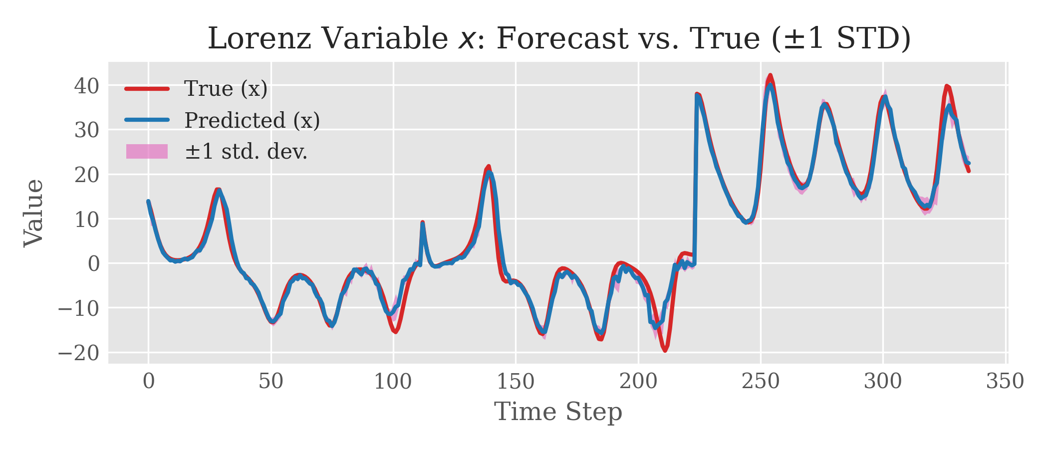
Figure 2: Forecasting performance of variable $x$ by FRIREN on sample 0 of the Lorenz63 system test set, over a 336-step prediction horizon.

Table 1: Comparative Performance Summary (Averaged over inputs 96 & 336 steps)

Dataset	Metric	FRI.	T.Mixer	TST.	DLin.
Lorenz63	MSE	19.40	24.76	26.16	63.55
	MAE	2.12	2.39	2.88	5.74
	SWD	1.89	3.85	4.72	21.96
Rossler	MSE	0.02	2.52	3.44	4.58
	MAE	0.07	0.64	0.82	0.88
	SWD	0.01	1.72	2.22	3.15
ETTm1	MSE	10.06	10.30	10.31	10.79
	MAE	1.70	1.66	1.76	1.66
	SWD	2.07	1.85	2.09	1.64
Weather*	MSE	0.25	0.24	0.25	0.23
	MAE	0.33	0.30	0.31	0.31
	SWD	0.09	0.08	0.09	0.10
Weather* results are avg. over Input 196 & 336 steps.

Let us focus on the Lorenz63 "butterfly" system. The most significant advantage occurs at prediction length 336: as shown in LABEL:app:tab:lorenz63, FRIREN achieved an MSE of $11.41$, MAE of $1.61$, and SWD of $0.97\pm 0.16$, substantially outperforming TimeMixer (MSE $27.33$, MAE $2.81$, SWD $2.09$) in the 336-input, 336-output, $dt=0.01$ setting. Figure˜2 illustrates our model’s performance on the first test sample. For state variable $x$, FRIREN captures the complex oscillations quite accurately, with only minor magnitude errors in a few places. For long-term performance across the entire test set, see Figure˜4 in the appendix.

Ablation Studies Summary

To validate the contributions of FRIREN’s core components, we conducted ablation studies on the Lorenz63 dataset (336-in, 336-out). Key results are presented in Table˜2, with the baseline representing the full FRIREN model. Each component proves indispensable: removing the ANF structure increases MSE by over 51% (from 24.50 to 37.06), while removing scale components increases MSE by 35%. The complete ablation results are presented in Appendix 12. Notably, while data-dependent shift contributes significantly to performance, the Koopman operator is not redundant—it independently improves results while providing interpretability benefits. Additionally, Huber loss provided a consistent advantage over standard MSE loss across all configurations (see Appendix 13 for detailed comparisons).

Table 2: Key Ablation Results on Lorenz63 (SeqLen=336, PredLen=336, dt=0.01 RK4, Unnormalized)

FRIREN Core Components Effectiveness	Test MSE ↓	Test MAE ↓	Test SWD ↓
Full FRIREN Model	24.50 $\pm$ 1.64	2.68 $\pm$ 0.13	1.88 $\pm$ 0.20
Remove Koopman on z-space	27.61 $\pm$ 3.39	2.82 $\pm$ 0.26	2.20 $\pm$ 0.50
Remove Rotation (pure ACL)	28.02 $\pm$ 1.35	2.89 $\pm$ 0.07	2.06 $\pm$ 0.21
Remove ANF ( $x\rightarrow z$ $\nrightarrow x\nrightarrow z$)	37.06 $\pm$ 2.08	3.35 $\pm$ 0.15	2.52 $\pm$ 0.51
Remove Scale Component in OT	33.02 $\pm$ 0.53	3.18 $\pm$ 0.09	1.96 $\pm$ 0.24
Remove Shift Component in OT	26.86 $\pm$ 1.52	2.75 $\pm$ 0.01	1.85 $\pm$ 0.37

Computational Resources

All experiments used a laptop with an NVIDIA mobile 4070 GPU (8GB VRAM). For a 52,000-step Lorenz63 dataset (336-in-336-out, 50 epochs, patience=5), training times were: FRIREN (16min), TimeMixer (21min), PatchTST (10min), and DLinear (2.5min). For ETTm1: FRIREN (83s), TimeMixer (120s), PatchTST (110s), and DLinear (27s). The project required 100-150 GPU hours total. Using THOP (Zhu, 2019), we measured model efficiency: FRIREN (1.025M params, 0.0035 GFLOPs), TimeMixer (0.886M params, 0.0463 GFLOPs), PatchTST (2.008M params, 0.0308 GFLOPs), and DLinear (0.679M params, 0.0007 GFLOPs).

Broader Impacts and Limitations

FRIREN is fundamentally a geometric and interpretable model for long-term time series forecasting (LTSF). Unlike standard black-box models, it is built around a linear transformation structure, with most components having a clear mathematical interpretation. FRIREN is thus uniquely interpretable at two levels: Globally, the Koopman operator allows practitioners to estimate, predict, and even control system behaviour based on the learned spectral properties. Locally, data-dependent scaling and translation allow direct checking of failure mode, making it valuable in fields where understanding why predictions fails matters more than a couple of percentage points better or worse than other state-of-the-arts models.

However, this geometric approach has its limits. FRIREN performs well on chaotic systems like Lorenz63, Rossler, the kind of dissipative chaotic system (one that loses energy over time) that has a compact attractor—meaning the system’s behaviour, while complex, remains confined to a bounded region of space rather than wandering indefinitely. Lorenz96 with $F=8$ has a quasi-stable behaviour, and our results are still better than other LTSF models (see LABEL:app:data:lorenz96_8). Empirically (results not included in this paper), when F = 15 — a regime of stronger forcing, more unstable directions and higher variance — our advantage shrinks. In the hyperchaotic regime (F = 24), FRIREN’s advantage diminishes, eventually performing on par with simpler models like DLinear. Without a stable geometric structure, such as in random walks, FRIREN cannot reliably learn meaningful dynamics.

This highlights a fundamental trade-off: FRIREN excels where systems have a learnable geometric structure but can struggle with highly stochastic or purely random systems. It is not a universal solution. Rather, it is part of a toolset for practitioners. Preliminary analysis on predictability cannot be replaced. Additionally, while our affine coupling layer ACL module $s(z)\cdot x+t(z)$ is robust and avoids the instability of $s(x)\cdot x+t(x)$, it still requires careful training. We use stabilizing techniques—ReLU6, spectral normalization, and specific activation functions—to maintain numerical stability.

In terms of scalability, FRIREN is efficient. It avoids expensive components, and the Householder rotations are lightweight. The primary computational cost arises from spectral normalization, which can slow down training but is essential for stability on some datasets. Finally, Our complete codebase is available at https://anonymous.4open.science/r/LTSF_model-03BB/ for reproducibility.

Appendix A Appendix

A.1 Experimental Setup Details

A.1.1 Implementation Details

All models were implemented in PyTorch. Training and evaluation were performed on a laptop with an NVIDIA mobile 4070 GPU. For synthetic datasets, trajectories were generated using the 4th-order Runge-Kutta (RK4) method with a time step $dt=0.01$, unless otherwise specified. Standard parameters were used for these systems as detailed below. For real-world benchmark datasets, we followed the standard data processing and train/validation/test splits (70%/10%/20% chronologically) used in the LTSF literature. Notably, we did not use drop_last flag for any data loader, and we did not use the Random seeds used for result averaging are [1955, 7, 20].

A.2 Dataset Descriptions

We evaluated our proposed model and baselines on a combination of synthetic chaotic systems and widely used real-world benchmark datasets.

A.2.1 Synthetic Chaotic Systems

These datasets allow for controlled evaluation of a model’s ability to capture complex, deterministic dynamics.

Lorenz63 System

A canonical 3-dimensional chaotic system modelling simplified atmospheric convection.

• Equations:

  $$\dot{x} =\sigma(y-x)$$

  $$\dot{y} =x(\rho-z)-y$$

  $$\dot{z} =xy-\beta z$$

• Parameters: Standard chaotic regime values $\sigma=10$, $\rho=28$, $\beta=8/3$.

• Initial Condition: $(1.0,0.98,1.1)$.

• Generation: RK4 integration with $dt=0.01$. Total length generated: 52,000 steps (after discarding initial transient).

• Task: Input length 336, predict next 336 steps.

Rossler System

A 3-dimensional chaotic system known for its simpler folded-band attractor structure.

• Equations:

  $$\dot{x} =-y-z$$

  $$\dot{y} =x+ay$$

  $$\dot{z} =b+z(x-c)$$

• Parameters: Standard values $a=0.2$, $b=0.2$, $c=5.7$.

• Initial Condition: $(1.0,1.0,1.0)$.

• Generation: RK4 integration with $dt=0.01$. Total length generated: 52,000 steps (after discarding initial transient).

• Task: Input length 336, predict next 336 steps.

Lorenz96 System

A higher-dimensional chaotic system modeling atmospheric dynamics across spatial locations.

• Equations: For $i=1,\dots,N$:

  $$\frac{dX_{i}}{dt}=(X_{i+1}-X_{i-2})X_{i-1}-X_{i}+F$$

  (Indices are taken modulo $N$).

• Parameters: Dimension $N=6$. We test forcing $F=8.0$ (classic chaotic setting) and $F=15.0$ (medium level chaotic behaviour).

• Initial Condition: $X_{i}=F$ for all $i$, except $X_{0}=F+0.01$.

• Generation: RK4 integration with $dt=0.01$. Total length generated: 19,000 steps (after discarding initial transient).

• Task: Input length 96, predict horizons {96, 192, 336, 720} steps.

A.2.2 Real-World Benchmark Datasets

These datasets are standard in the Long-Term Time Series Forecasting (LTSF) literature. It is worth mentioning that Hu et al. (2024) reported positive Lyapunov exponents for these datasets, indicating chaotic behavior.

ETT (Electricity Transformer Temperature)

Data was collected from two electricity transformers in China over 2 years.

• ETTm1: 7 variables, recorded every 15 minutes.

• ETTm2: 7 variables, recorded every 15 minutes.

• ETTh1: 7 variables, recorded every hour.

• ETTh2: 7 variables, recorded every hour.

• Task: Input length 336, predict horizons {96, 192, 336, 720} steps.

Weather

Contains 21 meteorological indicators (e.g., temperature, humidity) recorded every 10 minutes at the Max Planck Institute for Biogeochemistry weather station in Germany over 2020.

• Variables: 21.

• Frequency: 10 minutes.

• Task: Input length 336, predict horizons {96, 192, 336, 720} steps.

A.3 Evaluation Metrics

We evaluate forecasting performance using standard metrics:

• MSE: Mean Squared Error.

• MAE: Mean Absolute Error.

• SWD: Sliced Wasserstein Distance (SWD-2), calculated using $N=500$ random projections. For each projection direction $\theta_{i}$ (sampled uniformly from the unit hypersphere), the predicted and target distributions are projected onto this direction, transforming them into one-dimensional distributions. The Wasserstein-2 distance ($W_{2}$) is then calculated between the empirical quantiles of these 1D projections:

  $$\mathrm{SWD}^{2}(P,Q)=\frac{1}{N}\sum_{i=1}^{N}W_{2}^{2}\left(\operatorname{Quantile}\left(\langle X,\theta_{i}\rangle\right),\operatorname{Quantile}\left(\langle Y,\theta_{i}\rangle\right)\right)$$

  For the 1D case, $W_{2}$ is simply the squared Euclidean (L2) distance between the sorted quantiles:

  $$W_{2}^{2}\left(\operatorname{Quantile}(X),\operatorname{Quantile}(Y)\right)=\int_{0}^{1}\left[Q_{X}(t)-Q_{Y}(t)\right]^{2}\,dt$$

  where $Q_{X}(t)$ and $Q_{Y}(t)$ are the quantile functions of the projected distributions $X$ and $Y$, respectively. This formulation ensures that SWD-2 not only captures pointwise accuracy but also aligns the distributional shape of the predicted and target sequences.

Lower values are better for all metrics.

Huber Loss: A Stable Training Objective

The primary training objective was Huber loss with $\delta=1.0$. It combines the robustness of MAE with the sensitivity of MSE, penalizing errors quadratically for small differences and linearly for large ones. This dampens the influence of significant prediction deviations or outliers, enhancing training stability, which is particularly relevant for potentially noisy or chaotic datasets. Ablation studies (see Appendix 13) confirmed that adopting Huber loss improved performance over standard MSE for our model.

Effective Prediction Time (EPT)

For chaotic systems, we also report Effective Prediction Time (EPT). For each channel and test sequence, EPT is the first time step $s\in[1,H]$ where the absolute prediction error $|y_{pred,s}-y_{true,s}|$ exceeds a threshold $\epsilon$, typically set to one standard deviation of the true time series for that channel. If the error never exceeds $\epsilon$ within the horizon $H$, EPT is $H$. The reported EPT is the average over all test sequences and channels. EPT serves as a sanity-check for prediction uniformity, indicating the reliable prediction range for a model-dataset combination.

A.4 Model Hyperparameters

All models were trained using the AdamW optimizer with a learning rate of $9\times 10^{-4}$ and a batch size of 128 for 50 epochs, using Huber loss ($\delta=1.0$). Key hyperparameters for FRIREN include: hidden dimension (d_model) of 128, and 2 encoding layers in the Augmented Normalizing Flow blocks. The EigenACL component uses a configurable number of Householder reflections (typically 2-4, tuned per dataset group). The Koopman operator $K$, when used, has a latent dimension $h$ matching $d_{model}$.

For baseline models (PatchTST (Nie et al., 2022), DLinear (Zeng et al., 2023), TimeMixer (wangTimeMixerGeneralTime2025)), we adapted configurations from their original papers or common implementations. Table 3 summarizes key settings.

Table 3: Key Hyperparameters for Main Experiments in Appendix

Parameter	FRIREN	PatchTST	DLinear	TimeMixer
Optimizer	AdamW	AdamW	AdamW	AdamW
Learning Rate	$9\times 10^{-4}$	$9\times 10^{-4}$	$9\times 10^{-4}$	$9\times 10^{-4}$
Batch Size	128	128	128	128
Epochs	50	50	50	50
Loss Function	Huber	Huber	Huber	Huber
Huber Delta	1.0	1.0	1.0	1.0
Patch Length	N/A	16	N/A	N/A
Patch Stride	N/A	8	N/A	N/A
Hidden Dim ($d_{model}$)	128	128	N/A	16
FFN Dim ($d_{ff}$)	N/A	256	N/A	32
No. Heads	N/A	16	N/A	N/A
Dropout	0.2	0.2	N/A	0.1
Enc. Layers	2	3	N/A	2
Num. ANF Blocks	2	N/A	N/A	N/A
OT Householder Refl.	4	N/A	N/A	N/A
Koopman Householder Refl.	2	N/A	N/A	N/A
Down Samp. Layers	N/A	N/A	N/A	3
Down Samp. Window	N/A	N/A	N/A	2
Kernel Size	N/A	N/A	N/A	5

A.5 Visuals

A.5.1 Picture

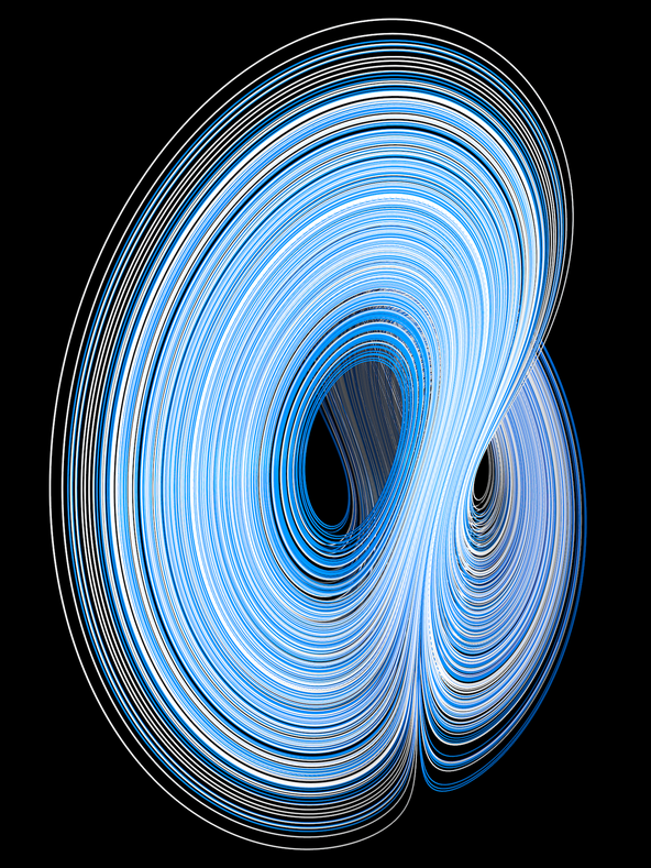
Figure 3: Lorenz attractor visualization. Image by Jos Leys, used under CC BY-NC-SA 3.0. Source: https://www.imaginary.org/gallery/the-lorenz-attractor

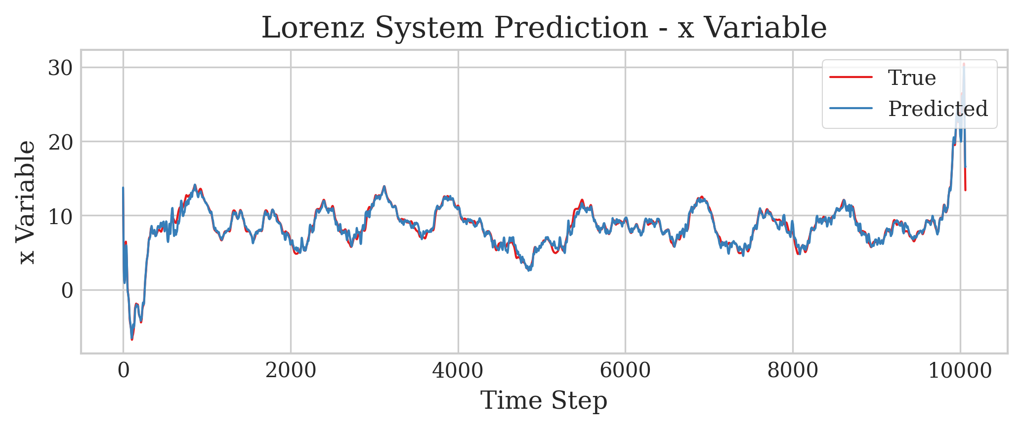
Figure 4: Continuous reconstruction of the full test trajectory (10 063 time steps) from the results using the first random seed. It shows the true (red) versus predicted (blue) series for the variables $x$.

A.6 Diagram

A.7 Definition, Theorem, Propositions

A.7.1 Takens Embedding Theorem

Theorem A.1 (Takens’ Embedding Theorem (Takens, 1981)).

Let $M$ be a compact manifold of dimension $d_{M}$. Consider a dynamical system described by a diffeomorphism $\phi:M\to M$ and a smooth scalar observation function $y:M\to\mathbb{R}$.

If the embedding dimension $m$ satisfies $m\geq 2d_{M}+1$, then the delay-coordinate map $\Phi:M\to\mathbb{R}^{m}$, defined by

$$\Phi(x)=\left(y(x),y(\phi^{-1}(x)),y(\phi^{-2}(x)),\dots,y(\phi^{-(m-1)}(x))\right)$$ (4)

is generically an embedding.

This implies that the reconstructed attractor in the $m$-dimensional delay-coordinate space is diffeomorphic to the original attractor on $M$, thus preserving its topological properties and dynamics.

A.7.2 Koopman Invariance

Consider a Hilbert space of functions with a chosen basis of observable functions $\{y_{1}(\mathbf{x}),y_{2}(\mathbf{x}),\ldots\}$. Any function $g(\mathbf{x})$ in this space can be written as:

$$g=\sum_{k=1}^{\infty}\alpha_{k}y_{k}.$$ (5)

A Koopman-invariant subspace is given by $\text{span}\{y_{s_{1}},y_{s_{2}},\cdots,y_{s_{m}}\}$ if all functions $g$ in this subspace,

$$g=\alpha_{1}y_{s_{1}}+\alpha_{2}y_{s_{2}}+\cdots+\alpha_{m}y_{s_{m}},$$ (6)

remain in this subspace after being acted on by the Koopman operator $\mathcal{K}$:

$$\mathcal{K}g=\beta_{1}y_{s_{1}}+\beta_{2}y_{s_{2}}+\cdots+\beta_{m}y_{s_{m}}.$$ (7)

A.7.3 Effective Prediction Time (EPT)

The Effective Prediction Time (EPT) is a metric used to quantify the duration for which a forecast remains reliable, particularly for chaotic dynamical systems (Wang and Li, 2024). It measures the time until the prediction error first surpasses a pre-defined threshold.

Let $y_{pred,d,s}$ be the predicted value for dimension (channel) $d$ at prediction step $s$ (out of a total horizon $H$), and $y_{true,d,s}$ be the corresponding true value. Let $\epsilon_{d}$ be the error threshold for dimension $d$, commonly set to one standard deviation of the true values for that dimension, $\sigma_{d}$. The EPT for a single sequence and a single dimension $d$ is defined as:

$$\text{EPT}_{d}=\min\{s\in[1,H]\mid|y_{pred,d,s}-y_{true,d,s}|>\epsilon_{d}\}$$ (8)

If $|y_{pred,d,s}-y_{true,d,s}|\leq\epsilon_{d}$ for all $s\in[1,H]$, then $\text{EPT}_{d}=H$.

The overall EPT reported is typically the average over all dimensions $D$ and all test sequences $B$ in the batch or evaluation set:

$$\text{EPT}_{\text{avg}}=\frac{1}{B\cdot D}\sum_{b=1}^{B}\sum_{d=1}^{D}\text{EPT}_{b,d}$$ (9)

Theorem A.2 (Brenier, McCann).

Let $\mu,\nu$ be probability measures on $\mathbb{R}^{n}$ with finite second moments. Assume $\mu$ is absolutely continuous w.r.t. the $n$-dimensional Lebesgue measure. For the quadratic cost $c(x,y)=\|x-y\|^{2}/2$, there exists a unique optimal transport map $T:\mathbb{R}^{n}\to\mathbb{R}^{n}$ such that $T_{\#}\mu=\nu$, and for some convex function $\psi:\mathbb{R}^{n}\to\mathbb{R}$

$$T(x)=\nabla\psi(x)\quad\text{for }\mu\text{-almost every }x.$$

Definition A.3 (Wasserstein-2).

$$W_{2}(\delta_{p},\nu)=\left(\inf_{\gamma\in\Pi(\delta_{p},\nu)}\int|x^{\prime}-y^{\prime}|^{2}d\gamma(x^{\prime},y^{\prime})\right)^{1/2}$$

Definition A.4.

$$W_{2}^{2}(\mu,\nu)=\int_{\mathbb{R}^{n}}\|x-T(x)\|^{2}d\mu(x)$$

Definition A.5 (Measure-Preserving Map).

$T:\mathbb{R}^{n}\to\mathbb{R}^{n}$ is a pushforward / transport of measure when $T_{\#}\mu=\nu$, meaning $\nu(B)=\mu(T^{-1}(B))$ for any set $B$.

Definition A.6 (Monotone).

Being monotone means for all $x,y$ in the domain

$$\langle\nabla f(x)-\nabla f(y),\,x-y\rangle\geq 0$$

Proposition A.7 (Convexity Function).

a continuously differentiable function function $f$ can be characterized as convex in two equivalent manners: (1) the gradient of $f$, $\nabla f$, is a monotone operator (2) the Hessian of $f$ (i.e. the Jacobian of the optimal transport mapping $\nabla f$) is symmetric and positive semi-definite (PSD) everywhere in the domain.

A.7.4 Justification: OT Property of Maps with Symmetric PSD Jacobians

We justify the claim that a sufficiently regular map $T:\mathbb{R}^{n}\to\mathbb{R}^{n}$ (e.g., $C^{1}$) with a symmetric positive semi-definite (PSD) Jacobian $DT(x)$ is the unique $W_{2}$-optimal transport map between a suitable source $\mu$ and the induced target $\nu=T_{\#}\mu$. The logic follows from combining standard results:

1. Gradient of a Convex Potential: If the Jacobian $DT(x)$ is symmetric everywhere on a simply connected domain like $\mathbb{R}^{n}$, the vector field $T$ is conservative. By the Poincaré lemma or fundamental theorem of calculus for line integrals, this ensures $T$ is the gradient of some scalar potential $\psi$ ($T=\nabla\psi$). Furthermore, if $DT=D^{2}\psi$ (the Hessian of $\psi$) is PSD, then $\psi$ is convex by definition. Thus, $T=\nabla\psi$ for some convex $\psi$.

2. Induced Target Measure: Given a source probability measure $\mu$, the map $T$ defines a unique pushforward probability measure $\nu=T_{\#}\mu$, which is the distribution of $T(x)$ when $x\sim\mu$. If $\mu$ has a finite second moment and $T$ is affine (as in the component maps $T_{z}$), $\nu$ also has a finite second moment.

3. Identification via Brenier’s Theorem: Assume $\mu$ satisfies the conditions for Brenier’s theorem (e.g., $\mu$ is absolutely continuous w.r.t. $\lambda^{n}$, has finite second moment). Let $\nu=T_{\#}\mu$. Brenier’s theorem (Brenier, 1991) (and McCann’s extension McCann (1995)) guarantees that for the quadratic cost $c(x,y)=\|x-y\|^{2}/2$, there exists a unique optimal transport map $T_{opt}:\mathbb{R}^{n}\to\mathbb{R}^{n}$ transporting $\mu$ to $\nu$, and this map must be the gradient of some convex potential $\psi_{opt}$.

   Since our map $T$ (from step a) is already $T=\nabla\psi$ for a convex $\psi$, and it transports $\mu$ to $\nu$ (step b), by the uniqueness of the optimal map, $T$ must be equal ($\mu$-a.e.) to $T_{opt}$.

4. Conclusion: Therefore, a map $T$ with a symmetric PSD Jacobian is precisely the unique $W_{2}$-optimal transport map between $\mu$ and its induced image measure $\nu=T_{\#}\mu$. It achieves the minimum $W_{2}$ cost for this specific transformation, which equals $W_{2}(\mu,\nu)^{2}$. Further details can be found in standard OT texts (Villani, 2008).

A.7.5 Justification: Equivalence of MSE and Point-Predictor W2 Objectives

Proposition A.8 (Equivalence of MSE and Point-Predictor W2 Objectives).

Let $x\in\mathcal{X}$ be an input variable, and $y\in\mathcal{Y}\subseteq\mathbb{R}^{n}$ be the target variable following a true conditional distribution $P(y|x)$ with a well-defined conditional mean $m(x)=\mathbb{E}[y|x]$. Consider a deterministic predictor function $p:\mathcal{X}\to\mathcal{Y}$ that outputs a point prediction $y_{\text{pred}}=p(x)$. Let $L_{\text{MSE}}(p)=\mathbb{E}_{x,y}[\|p(x)-y\|^{2}]$ be the expected Mean Squared Error. Let $L_{W2\delta}(p)=\mathbb{E}_{x}[W_{2}^{2}(\delta_{p(x)},P(y|x))]$ be the expected squared Wasserstein-2 distance between the predictor’s output (as a Dirac measure) and the true conditional distribution.

Then, minimizing $L_{\text{MSE}}(p)$ and minimizing $L_{W2\delta}(p)$ with respect to the function $p(x)$ yield the same unique optimal predictor: $p^{*}(x)=m(x)=\mathbb{E}[y|x]$.

A.7.6 MSE Loss Decomposition

Let the model prediction be $\mathbf{f}(\mathbf{x},\mathbf{z})$, depending on input $\mathbf{x}$ and internal randomness $\mathbf{z}\sim p(\mathbf{z})$. Let the true data be $\mathbf{y}\sim p(\mathbf{y}|\mathbf{x})$. We analyze the conditional expected MSE loss $L_{\mathbf{x}}$ for a fixed $\mathbf{x}$.

Step 1: Definition and Iterated Expectation

The loss is the expectation over both sources of randomness:

$$L_{\mathbf{x}}=\mathbb{E}_{\mathbf{z},\mathbf{y}}\left[\|\mathbf{f}(\mathbf{x},\mathbf{z})-\mathbf{y}\|^{2}\right]=\mathbb{E}_{\mathbf{z}}\left[\mathbb{E}_{\mathbf{y}|\mathbf{x}}\left[\|\mathbf{f}(\mathbf{x},\mathbf{z})-\mathbf{y}\|^{2}\right]\right]$$ (10)

Step 2: Decompose Inner Expectation (over $\mathbf{y}$)

Let $m(\mathbf{x})=\mathbb{E}[\mathbf{y}|\mathbf{x}]$ be the true conditional mean. For a fixed prediction $p=\mathbf{f}(\mathbf{x},\mathbf{z})$, the inner expectation is:

$$\mathbb{E}_{\mathbf{y}|\mathbf{x}}\left[\|\mathbf{f}(\mathbf{x},\mathbf{z})-\mathbf{y}\|^{2}\right] =\|\mathbf{f}(\mathbf{x},\mathbf{z})-m(\mathbf{x})\|^{2}+\mathbb{E}_{\mathbf{y}|\mathbf{x}}[\|\mathbf{y}-m(\mathbf{x})\|^{2}]$$

$$=\|\mathbf{f}(\mathbf{x},\mathbf{z})-m(\mathbf{x})\|^{2}+\text{Var}(\mathbf{y}|\mathbf{x})$$

Here, $\text{Var}(\mathbf{y}|\mathbf{x})$ is the irreducible variance of the true data given $\mathbf{x}$.

Step 3: Substitute Back and Focus on Expectation over $\mathbf{z}$

Plugging this back into the expression for $L_{\mathbf{x}}$:

$$L_{\mathbf{x}} =\mathbb{E}_{\mathbf{z}}\left[\|\mathbf{f}(\mathbf{x},\mathbf{z})-m(\mathbf{x})\|^{2}+\text{Var}(\mathbf{y}|\mathbf{x})\right]$$

$$=\mathbb{E}_{\mathbf{z}}\left[\|\mathbf{f}(\mathbf{x},\mathbf{z})-m(\mathbf{x})\|^{2}\right]+\text{Var}(\mathbf{y}|\mathbf{x})\quad(\text{since }\text{Var}(\mathbf{y}|\mathbf{x})\text{ is constant w.r.t. }\mathbf{z})$$

Step 4: Decompose Remaining Expectation (over $\mathbf{z}$)

Let $p(\mathbf{x})=\mathbb{E}_{\mathbf{z}}[\mathbf{f}(\mathbf{x},\mathbf{z})]$ be the mean prediction (averaged over $\mathbf{z}$). We analyze the term $\mathbb{E}_{\mathbf{z}}[\|\mathbf{f}(\mathbf{x},\mathbf{z})-m(\mathbf{x})\|^{2}]$. This is the expected squared distance between the stochastic prediction $\mathbf{f}(\mathbf{x},\mathbf{z})$ and the fixed true mean $m(\mathbf{x})$. Using the property $\mathbb{E}[\|X-c\|^{2}]=\|\mathbb{E}[X]-c\|^{2}+\text{Var}(X)$:

$$\mathbb{E}_{\mathbf{z}}\left[\|\mathbf{f}(\mathbf{x},\mathbf{z})-m(\mathbf{x})\|^{2}\right] =\|\underbrace{\mathbb{E}_{\mathbf{z}}[\mathbf{f}(\mathbf{x},\mathbf{z})]}_{p(\mathbf{x})}-m(\mathbf{x})\|^{2}+\underbrace{\mathbb{E}_{\mathbf{z}}[\|\mathbf{f}(\mathbf{x},\mathbf{z})-\mathbb{E}_{\mathbf{z}}[\mathbf{f}(\mathbf{x},\mathbf{z})]\|^{2}]}_{\text{Var}_{\mathbf{z}}(\mathbf{f}(\mathbf{x},\mathbf{z}))}$$

$$=\|p(\mathbf{x})-m(\mathbf{x})\|^{2}+\text{Var}_{\mathbf{z}}(\mathbf{f}(\mathbf{x},\mathbf{z}))$$

Step 5: Final Decomposition of $L_{\mathbf{x}}$

Combining the results:

$$L_{\mathbf{x}}=\underbrace{\|p(\mathbf{x})-m(\mathbf{x})\|^{2}}_{\text{(A) Squared Error of Mean Pred.}}+\underbrace{\text{Var}_{\mathbf{z}}(\mathbf{f}(\mathbf{x},\mathbf{z}))}_{\text{(B) Variance due to }\mathbf{z}}+\underbrace{\text{Var}(\mathbf{y}|\mathbf{x})}_{\text{(C) Irreducible Error}}$$ (11)

Conclusion: Minimizing the expected MSE $L_{\mathbf{x}}$ requires minimizing both (A) the squared error of the mean prediction and (B) the variance introduced by the model’s internal randomness $\mathbf{z}$. Thus, MSE incentivizes the model to produce predictions that are effectively deterministic conditional mean estimates.

A.8 Results

A.8.1 Lorenz63

Table 4: Performance (3-seed ([1955, 7, 20]) average $\pm$ std. dev.) on dataset Lorenz (Unnormalized Data Only, dt=1e-2, steps=52000, parameters $\sigma=10.0,\rho=28.0,\beta=8/3$; )

Seq.Len	Pred.Len	Model	MSE	MAE	SWD	EPT
Input Sequence Length: 96
Unnormalized Data (scale=False)
96	96	FRIREN	$1.0112\pm 0.2211$	$0.4649\pm 0.0153$	$0.2421\pm 0.0195$	$95.3839\pm 0.1269$
		TimeMixer	$3.6820\pm 1.2307$	$0.8703\pm 0.1994$	$1.1182\pm 0.2519$	$93.1517\pm 1.0061$
		PatchTST	$3.1388\pm 0.5167$	$0.8923\pm 0.0816$	$0.8851\pm 0.2039$	$94.0470\pm 0.3028$
		DLinear	$56.7910\pm 0.4369$	$5.0559\pm 0.0207$	$16.1738\pm 0.3259$	$50.5227\pm 0.5466$
	196	FRIREN	$4.2496\pm 0.7186$	$0.9425\pm 0.1248$	$0.5145\pm 0.1352$	$184.2673\pm 2.5229$
		TimeMixer	$13.4769\pm 2.0056$	$1.9334\pm 0.1798$	$2.2558\pm 0.1897$	$167.5430\pm 3.4347$
		PatchTST	$12.8054\pm 1.0178$	$1.9406\pm 0.0964$	$2.4246\pm 0.2857$	$167.8815\pm 1.5703$
		DLinear	$63.3469\pm 0.1008$	$5.6401\pm 0.0044$	$20.6054\pm 0.4115$	$56.0611\pm 0.1487$
	336	FRIREN	$23.7017\pm 2.9601$	$2.7683\pm 0.2577$	$2.5651\pm 0.7043$	$213.8304\pm 14.4593$
		TimeMixer	$30.7690\pm 0.8496$	$3.3360\pm 0.0640$	$4.8611\pm 1.2307$	$207.9292\pm 6.0368$
		PatchTST	$31.5992\pm 0.7597$	$3.3713\pm 0.0487$	$5.4578\pm 0.2636$	$203.3673\pm 2.2813$
		DLinear	$66.0108\pm 0.1827$	$5.9360\pm 0.0078$	$24.4054\pm 0.4662$	$57.7992\pm 0.4087$
	720	FRIREN	$47.2386\pm 0.9446$	$4.3913\pm 0.1105$	$5.7438\pm 0.6005$	$247.5058\pm 10.0393$
		TimeMixer	$51.1233\pm 1.7998$	$4.8833\pm 0.1404$	$11.9739\pm 1.3537$	$204.3494\pm 14.5916$
		PatchTST	$52.1294\pm 0.9395$	$4.9760\pm 0.0972$	$10.0533\pm 1.7525$	$200.0095\pm 12.2062$
		DLinear	$68.6638\pm 0.1640$	$6.2439\pm 0.0058$	$29.1775\pm 0.1888$	$56.8681\pm 1.4674$
Input Sequence Length: 336
Unnormalized Data (scale=False)
336	96	FRIREN	$2.3654\pm 0.5275$	$0.7475\pm 0.0955$	$0.5015\pm 0.0536$	$94.2000\pm 0.4771$
		TimeMixer	$2.9680\pm 0.3676$	$0.7235\pm 0.0482$	$0.8260\pm 0.1559$	$94.0752\pm 0.1751$
		PatchTST	$5.4495\pm 0.9481$	$1.3207\pm 0.1630$	$0.9258\pm 0.1472$	$92.7656\pm 0.6375$
		DLinear	$58.5568\pm 0.3109$	$5.3589\pm 0.0333$	$17.0806\pm 1.0705$	$48.1191\pm 1.0947$
	196	FRIREN	$4.3393\pm 0.6710$	$0.9808\pm 0.0839$	$0.5530\pm 0.1002$	$183.1031\pm 1.9392$
		TimeMixer	$5.1257\pm 0.3356$	$0.9558\pm 0.0550$	$0.6143\pm 0.0299$	$185.2168\pm 0.6879$
		PatchTST	$12.5343\pm 2.2358$	$1.9268\pm 0.1863$	$2.2511\pm 0.3257$	$169.2482\pm 4.3749$
		DLinear	$62.2699\pm 0.3688$	$5.6209\pm 0.0116$	$19.7883\pm 0.2781$	$56.9820\pm 0.7557$
	336	FRIREN	$11.4145\pm 1.2282$	$1.6146\pm 0.1313$	$0.9656\pm 0.1587$	$274.5805\pm 7.4334$
		TimeMixer	$27.3345\pm 6.2030$	$2.8132\pm 0.3579$	$2.0949\pm 0.1593$	$207.9292\pm 6.0368$
		PatchTST	$32.8696\pm 1.1018$	$3.3221\pm 0.1157$	$3.5280\pm 0.3079$	$217.9181\pm 3.4628$
		DLinear	$65.3914\pm 0.1545$	$5.9029\pm 0.0071$	$21.9630\pm 0.3026$	$60.1228\pm 0.4986$
	720	FRIREN	$59.8581\pm 0.8081$	$4.9497\pm 0.0285$	$3.9214\pm 0.4480$	$225.7067\pm 1.9141$
		TimeMixer	$63.6242\pm 0.9433$	$5.4601\pm 0.0505$	$7.0515\pm 2.6831$	$189.1650\pm 28.8411$
		PatchTST	$59.7778\pm 0.5504$	$5.4001\pm 0.0352$	$10.0533\pm 1.7525$	$176.8817\pm 13.1934$
		DLinear	$67.3741\pm 0.4980$	$6.1861\pm 0.0251$	$26.4637\pm 0.4778$	$57.3006\pm 0.8426$
Average Performance for Input Length 96 (Unnormalized)
Input Length	Prediction Length	Model	Avg. MSE	Avg. MAE	Avg. SWD	Avg. EPT
96	-	FRIREN	$19.0503$	$2.1418$	$2.2664$	$185.2469$
		TimeMixer	$24.7628$	$2.7558$	$5.0523$	$168.2433$
		PatchTST	$24.6682$	$2.7701$	$4.7053$	$176.2164$
		DLinear	$63.7031$	$5.7190$	$22.5905$	$55.3128$
Average Performance for Input Length 336 (Unnormalized)
Input Length	Prediction Length	Model	Avg. MSE	Avg. MAE	Avg. SWD	Avg. EPT
336	-	FRIREN	$19.7400$	$2.0971$	$1.5189$	$193.2157$
		TimeMixer	$24.7631$	$2.0182$	$2.6467$	$169.0966$
		PatchTST	$27.6578$	$2.9924$	$4.7291$	$163.1815$
		DLinear	$63.3981$	$5.7672$	$21.3239$	$55.6311$
Overall Average Performance (Input 96 & 336, Unnormalized)
Input Length	Prediction Length	Model	Avg. MSE	Avg. MAE	Avg. SWD	Avg. EPT
96+336	-	FRIREN	$19.3951$	$2.1195$	$1.8927$	$189.2313$
		TimeMixer	$24.7629$	$2.3870$	$3.8495$	$168.6699$
		PatchTST	$26.1630$	$2.8812$	$4.7172$	$165.4000$
		DLinear	$63.5506$	$5.7431$	$21.9572$	$55.4719$

A.8.2 Rossler

Table 5: Performance (3-seed ([1955, 7, 20]) average $\pm$ std. dev.) on dataset Rossler(Unnormalized Data Only, dt=1e-2, steps=52000, )

Seq.Len	Pred.Len	Model	MSE	MAE	SWD	EPT
Input Sequence Length: 96
Unnormalized Data (scale=False)
96	96	FRIREN	$0.0063\pm 0.0017$	$0.0510\pm 0.0086$	$0.0039\pm 0.0010$	$96.0000\pm 0.0000$
		TimeMixer	$0.7042\pm 0.2293$	$0.2412\pm 0.0446$	$0.5304\pm 0.1503$	$95.0454\pm 0.2411$
		PatchTST	$0.8551\pm 0.2157$	$0.3049\pm 0.0554$	$0.6538\pm 0.2179$	$94.8934\pm 0.2169$
		DLinear	$1.7967\pm 0.0056$	$0.3534\pm 0.0018$	$1.4215\pm 0.0570$	$93.7704\pm 0.0158$
	196	FRIREN	$0.0181\pm 0.0042$	$0.0769\pm 0.0068$	$0.0114\pm 0.0034$	$195.9988\pm 0.0016$
		TimeMixer	$2.5285\pm 0.2754$	$0.5179\pm 0.0561$	$2.1432\pm 0.2093$	$188.0716\pm 1.1346$
		PatchTST	$3.1459\pm 0.5099$	$0.6975\pm 0.0616$	$2.3850\pm 0.4256$	$186.9184\pm 1.4540$
		DLinear	$4.2080\pm 0.0090$	$0.7247\pm 0.0017$	$3.5051\pm 0.1642$	$183.8405\pm 0.0399$
	336	FRIREN	$0.0349\pm 0.0231$	$0.0953\pm 0.0199$	$0.0170\pm 0.0138$	$334.5515\pm 1.7118$
		TimeMixer	$4.3988\pm 0.4557$	$0.8863\pm 0.0563$	$3.2065\pm 0.2390$	$300.6456\pm 0.6511$
		PatchTST	$5.5064\pm 0.5389$	$1.1477\pm 0.0742$	$3.7213\pm 0.3017$	$300.6456\pm 0.6511$
		DLinear	$5.4518\pm 0.0204$	$1.0274\pm 0.0164$	$3.7048\pm 0.0272$	$297.4221\pm 0.7319$
	720	FRIREN	$0.0591\pm 0.0114$	$0.1422\pm 0.0112$	$0.0231\pm 0.0041$	$706.6850\pm 7.7466$
		TimeMixer	$5.7667\pm 0.2532$	$1.2087\pm 0.0420$	$3.6217\pm 0.0678$	$587.7859\pm 4.1672$
		PatchTST	$6.7297\pm 0.5812$	$1.4188\pm 0.0884$	$3.7606\pm 0.2811$	$569.2163\pm 12.6910$
		DLinear	$6.9724\pm 0.0375$	$1.4038\pm 0.0033$	$4.0184\pm 0.0720$	$561.1814\pm 1.8886$
Input Sequence Length: 336
Unnormalized Data (scale=False)
336	96	FRIREN	$0.0103\pm 0.0038$	$0.0648\pm 0.0105$	$0.0073\pm 0.0036$	$96.0000\pm 0.0000$
		TimeMixer	$1.2084\pm 0.4278$	$0.4019\pm 0.0326$	$0.9493\pm 0.3146$	$94.2858\pm 0.4247$
		PatchTST	$1.3989\pm 0.3620$	$0.5238\pm 0.0649$	$0.9956\pm 0.3167$	$94.0051\pm 0.5426$
		DLinear	$1.8980\pm 0.0425$	$0.4027\pm 0.0170$	$1.5048\pm 0.1034$	$93.6115\pm 0.0561$
	196	FRIREN	$0.0069\pm 0.0021$	$0.0500\pm 0.0074$	$0.0033\pm 0.0009$	$196.0000\pm 0.0000$
		TimeMixer	$1.2231\pm 0.1147$	$0.4485\pm 0.0339$	$0.8994\pm 0.1207$	$188.9314\pm 0.4425$
		PatchTST	$2.2919\pm 0.4740$	$0.5681\pm 0.0668$	$1.8586\pm 0.5062$	$188.5503\pm 1.3036$
		DLinear	$3.9438\pm 0.0490$	$0.7375\pm 0.0116$	$3.1948\pm 0.1478$	$183.9378\pm 0.1273$
	336	FRIREN	$0.0107\pm 0.0025$	$0.0624\pm 0.0047$	$0.0055\pm 0.0013$	$336.0000\pm 0.0000$
		TimeMixer	$1.6001\pm 0.1871$	$0.5826\pm 0.0727$	$0.9594\pm 0.1590$	$319.2823\pm 4.4003$
		PatchTST	$3.3916\pm 0.1686$	$0.8209\pm 0.0255$	$2.3486\pm 0.1283$	$308.1135\pm 1.0700$
		DLinear	$5.4518\pm 0.0204$	$1.0274\pm 0.0164$	$3.7048\pm 0.0272$	$297.4221\pm 0.7319$
	720	FRIREN	$0.0092\pm 0.0035$	$0.0615\pm 0.0112$	$0.0037\pm 0.0013$	$719.4792\pm 0.3957$
		TimeMixer	$2.7076\pm 0.3168$	$0.7936\pm 0.0661$	$1.4854\pm 0.2506$	$626.3566\pm 11.3725$
		PatchTST	$4.1788\pm 0.2951$	$1.0662\pm 0.0460$	$2.0194\pm 0.1188$	$597.0664\pm 5.4990$
		DLinear	$6.5224\pm 0.0358$	$1.3680\pm 0.0040$	$3.8097\pm 0.0292$	$555.6938\pm 0.8297$
Average Performance for Input Length 96 (Unnormalized)
Input Length	Prediction Length	Model	Avg. MSE	Avg. MAE	Avg. SWD	Avg. EPT
96		FRIREN	$0.02693$	$0.0851$	$0.0121$	$333.3088$
		TimeMixer	$3.3496$	$0.7135$	$2.3755$	$293.9924$
		PatchTST	$4.0593$	$0.8922$	$2.6302$	$287.9184$
		DLinear	$4.6960$	$0.8785$	$3.2390$	$284.7073$
Average Performance for Input Length 336 (Unnormalized)
Input Length	Prediction Length	Model	Avg. MSE	Avg. MAE	Avg. SWD	Avg. EPT
336		FRIREN	$0.0093$	$0.0597$	$0.0050$	$336.8698$
		TimeMixer	$1.6848$	$0.5567$	$1.0734$	$307.2140$
		PatchTST	$2.8153$	$0.7448$	$1.8056$	$296.9338$
		DLinear	$4.4540$	$0.8839$	$3.0535$	$282.6663$
Overall Average Performance (Input 96 & 336, Unnormalized)
Input Length	Prediction Length	Model	Avg. MSE	Avg. MAE	Avg. SWD	Avg. EPT
96+336		FRIREN	$0.0181$	$0.0724$	$0.0085$	$335.0893$
		TimeMixer	$2.5172$	$0.6351$	$1.7244$	$300.6032$
		PatchTST	$3.4373$	$0.8185$	$2.2179$	$292.4261$
		DLinear	$4.5750$	$0.8812$	$3.1463$	$283.6868$

A.8.3 Lorenz96-Forcing=8

Table 6: Performance (3-seed average $\pm$ std. dev.) on dataset Lorenz96 (Unnormalized Data Only, $F=8.0$, dt=1e-2, steps=19000, n=6 dimensional system instead of 40)

In. Len.	Pred. Len.	Model	MSE	MAE	SWD	EPT
Input Sequence Length: 96
Unnormalized Data (scale=False)
96	96	FRIREN	$4.3302\pm 0.0726$	$1.3462\pm 0.0051$	$0.9390\pm 0.0405$	$69.2855\pm 0.2294$
		TimeMixer	$7.2533\pm 0.1799$	$1.8292\pm 0.0391$	$1.8931\pm 0.0409$	$72.5250\pm 0.7027$
		PatchTST	$5.9886\pm 0.1334$	$1.6199\pm 0.0073$	$1.6165\pm 0.1269$	$73.5349\pm 0.4474$
		DLinear	$6.1479\pm 0.1035$	$1.6869\pm 0.0207$	$1.1489\pm 0.0408$	$71.6910\pm 0.4186$
	196	FRIREN	$8.8996\pm 0.1281$	$2.1005\pm 0.0223$	$1.2706\pm 0.0376$	$81.0132\pm 0.7023$
		TimeMixer	$11.1851\pm 0.1894$	$2.4564\pm 0.0292$	$2.3409\pm 0.0903$	$91.6087\pm 3.9011$
		PatchTST	$10.3982\pm 0.5181$	$2.3778\pm 0.0941$	$1.7096\pm 0.1718$	$83.8736\pm 3.1093$
		DLinear	$10.1630\pm 0.1293$	$2.3228\pm 0.0174$	$1.5058\pm 0.0328$	$84.0696\pm 0.9318$
	336	FRIREN	$11.3114\pm 0.0640$	$2.5516\pm 0.0085$	$1.8095\pm 0.0743$	$101.8015\pm 2.3346$
		TimeMixer	$13.3878\pm 0.0611$	$2.8077\pm 0.0062$	$2.6423\pm 0.0863$	$91.8578\pm 1.6738$
		PatchTST	$13.2978\pm 0.1343$	$2.7812\pm 0.0137$	$1.8270\pm 0.0453$	$93.6092\pm 1.0245$
		DLinear	$12.7459\pm 0.0319$	$2.7741\pm 0.0044$	$3.6713\pm 0.1868$	$93.0195\pm 0.5456$
	720	FRIREN	$13.5167\pm 0.0420$	$2.9008\pm 0.0039$	$2.5698\pm 0.0658$	$61.9939\pm 4.0366$
		TimeMixer	$15.0277\pm 0.0695$	$3.0937\pm 0.0114$	$2.8122\pm 0.1300$	$86.6012\pm 1.9939$
		PatchTST	$13.8220\pm 0.2200$	$2.9936\pm 0.0000$	$2.0709\pm 0.1718$	$90.4955\pm 1.3161$
		DLinear	$13.8220\pm 0.2200$	$2.9936\pm 0.0000$	$3.8189\pm 0.1718$	$66.8233\pm 1.3153$
Input Sequence Length: 336
Unnormalized Data (scale=False)
336	96	FRIREN	$5.7899\pm 0.0770$	$1.5954\pm 0.0197$	$1.1503\pm 0.0658$	$74.9139\pm 0.7718$
		TimeMixer	$8.2882\pm 0.7073$	$2.0426\pm 0.1227$	$2.1169\pm 0.4048$	$64.6972\pm 4.0665$
		PatchTST	$5.7456\pm 0.2183$	$1.6518\pm 0.0389$	$1.4505\pm 0.1269$	$76.2243\pm 0.6674$
		DLinear	$10.0714\pm 0.0648$	$2.3307\pm 0.0023$	$3.1504\pm 0.1137$	$58.0789\pm 0.1522$
	196	FRIREN	$10.4220\pm 0.3497$	$2.4199\pm 0.0949$	$1.9071\pm 0.3525$	$76.5531\pm 10.2590$
		TimeMixer	$11.7716\pm 0.1942$	$2.5964\pm 0.0412$	$2.3840\pm 0.1431$	$72.7980\pm 4.0358$
		PatchTST	$10.3982\pm 0.5181$	$2.3778\pm 0.0941$	$1.7096\pm 0.1718$	$92.9561\pm 9.1795$
		DLinear	$12.0251\pm 0.2449$	$2.6815\pm 0.0232$	$3.4687\pm 0.2573$	$66.5479\pm 0.2324$
	336	FRIREN	$12.1953\pm 0.1752$	$2.7255\pm 0.0455$	$2.4803\pm 0.3411$	$70.9905\pm 8.5836$
		TimeMixer	$13.9587\pm 0.1961$	$2.9267\pm 0.0182$	$2.4241\pm 0.3871$	$66.1581\pm 0.6715$
		PatchTST	$13.4666\pm 0.1343$	$2.7998\pm 0.0137$	$1.8169\pm 0.0453$	$95.2396\pm 1.8631$
		DLinear	$13.2813\pm 0.0762$	$2.8805\pm 0.0106$	$3.2052\pm 0.0984$	$65.5581\pm 0.5990$
	720	FRIREN	$13.7868\pm 0.0358$	$2.9756\pm 0.0017$	$2.9640\pm 0.1137$	$61.9939\pm 4.0366$
		TimeMixer	$15.0277\pm 0.0695$	$3.0937\pm 0.0114$	$2.8122\pm 0.1300$	$65.2673\pm 3.3321$
		PatchTST	$15.3028\pm 0.1478$	$3.0912\pm 0.0102$	$2.4025\pm 0.1661$	$88.9651\pm 1.5648$
		DLinear	$14.7433\pm 0.0505$	$3.0873\pm 0.0054$	$3.5182\pm 0.1176$	$65.0364\pm 0.1720$
Average Performance Across Prediction Lengths (Unnormalized Data Only, Best Validation)
In. Len.	Data Type	Model	Avg. MSE	Avg. MAE	Avg. SWD	Avg. EPT
96		FRIREN	$9.5145$	$2.2248$	$1.6472$	$78.5235$
		TimeMixer	$11.7135$	$2.5468$	$2.4221$	$85.6482$
		PatchTST	$10.8767$	$2.4431$	$1.8060$	$85.3783$
		DLinear	$10.7197$	$2.4444$	$2.5362$	$78.9009$
336		FRIREN	$10.5485$	$2.4291$	$2.1254$	$71.1129$
		TimeMixer	$12.2616$	$2.6649$	$2.4343$	$67.2302$
		PatchTST	$11.2283$	$2.4802$	$1.8449$	$88.3463$
		DLinear	$12.5303$	$2.7450$	$3.3356$	$63.8053$
Avg. 96 & 336		FRIREN	$10.0315$	$2.3270$	$1.8863$	$74.8182$
		TimeMixer	$11.9876$	$2.6059$	$2.4282$	$76.4392$
		PatchTST	$11.0525$	$2.4617$	$1.8255$	$86.8623$
		DLinear	$11.6250$	$2.5947$	$2.9359$	$71.3531$

A.8.4 ETTm1

Table 7: Performance (3-seed ([1955, 7, 20]) average $\pm$ std. dev.) on dataset ETTm1 (Unnormalized Data Only)

Seq.Len	Pred.Len	Model	MSE	MAE	SWD
Input Sequence Length: 96
Unnormalized Data (scale=False)
96	96	FRIREN	$8.1527\pm 0.1010$	$1.4783\pm 0.0073$	$1.7269\pm 0.0802$
		TimeMixer	$8.0476\pm 0.0375$	$1.3997\pm 0.0037$	$1.4379\pm 0.0512$
		PatchTST	$8.0957\pm 0.1097$	$1.4240\pm 0.0189$	$1.6321\pm 0.0411$
		DLinear	$8.2920\pm 0.0684$	$1.4037\pm 0.0051$	$1.2948\pm 0.0475$
	196	FRIREN	$10.3759\pm 0.3400$	$1.6884\pm 0.0351$	$2.0083\pm 0.0994$
		TimeMixer	$10.3354\pm 0.1277$	$1.6086\pm 0.0134$	$1.7417\pm 0.1439$
		PatchTST	$10.3130\pm 0.0548$	$1.6429\pm 0.0042$	$2.0279\pm 0.0789$
		DLinear	$10.6750\pm 0.0337$	$1.5980\pm 0.0034$	$1.5555\pm 0.0373$
	336	FRIREN	$11.9608\pm 0.0863$	$1.8372\pm 0.0075$	$2.3656\pm 0.1460$
		TimeMixer	$12.3451\pm 0.0635$	$1.7845\pm 0.0024$	$2.0290\pm 0.0814$
		PatchTST	$12.1807\pm 0.2380$	$2.3746\pm 0.2037$	$2.0113\pm 0.1443$
		DLinear	$12.8139\pm 0.0382$	$1.7758\pm 0.0010$	$1.8027\pm 0.0447$
	720	FRIREN	$13.1695\pm 0.2006$	$1.9993\pm 0.0175$	$2.4797\pm 0.1562$
		TimeMixer	$13.2973\pm 0.1474$	$1.9687\pm 0.0177$	$2.4469\pm 0.1687$
		PatchTST	$13.3853\pm 0.0135$	$1.9762\pm 0.0133$	$2.5954\pm 0.2217$
		DLinear	$14.1613\pm 0.0995$	$1.9505\pm 0.0068$	$1.9712\pm 0.0841$
Input Sequence Length: 336
Unnormalized Data (scale=False)
336	96	FRIREN	$7.5682\pm 0.0624$	$1.4391\pm 0.0071$	$1.7074\pm 0.1254$
		TimeMixer	$7.3753\pm 0.0846$	$1.3772\pm 0.0045$	$1.4542\pm 0.0796$
		PatchTST	$7.7119\pm 0.1559$	$1.4361\pm 0.0179$	$1.7424\pm 0.0793$
		DLinear	$7.8549\pm 0.0287$	$1.3890\pm 0.0030$	$1.3324\pm 0.0497$
	196	FRIREN	$8.7744\pm 0.1230$	$1.5738\pm 0.0041$	$1.8310\pm 0.0734$
		TimeMixer	$9.2151\pm 0.0234$	$1.5601\pm 0.0061$	$1.6314\pm 0.0838$
		PatchTST	$9.3505\pm 0.1502$	$1.6205\pm 0.0248$	$2.1119\pm 0.2233$
		DLinear	$9.6525\pm 0.0300$	$1.5707\pm 0.0029$	$1.5965\pm 0.0477$
	336	FRIREN	$9.8562\pm 0.1165$	$1.7206\pm 0.0063$	$2.1384\pm 0.1340$
		TimeMixer	$10.4413\pm 0.1240$	$1.7039\pm 0.0065$	$1.8461\pm 0.0461$
		PatchTST	$10.4511\pm 0.3693$	$1.7451\pm 0.0172$	$2.2369\pm 0.1096$
		DLinear	$10.9572\pm 0.0571$	$1.7158\pm 0.0043$	$1.7673\pm 0.0575$
	720	FRIREN	$10.6227\pm 0.1898$	$1.8495\pm 0.0074$	$2.2832\pm 0.1290$
		TimeMixer	$11.3628\pm 0.1597$	$1.8738\pm 0.0211$	$2.2133\pm 0.2582$
		PatchTST	$10.9889\pm 0.2663$	$1.8802\pm 0.0244$	$2.3854\pm 0.3386$
		DLinear	$11.9146\pm 0.0538$	$1.8526\pm 0.0046$	$1.8133\pm 0.0499$
Average Performance Across Prediction Lengths (Unnormalized Data Only)
Input Length	Data Type	Model	Avg. MSE	Avg. MAE	Avg. SWD
96		FRIREN	$10.9147$	$1.7508$	$2.1451$
		TimeMixer	$11.0064$	$1.6904$	$1.9139$
		PatchTST	$10.9937$	$1.7154$	$2.1575$
		DLinear	$11.4856$	$1.6820$	$1.6561$
336		FRIREN	$9.2054$	$1.6458$	$1.9900$
		TimeMixer	$9.5986$	$1.6288$	$1.7863$
		PatchTST	$9.6256$	$1.6705$	$2.1192$
		DLinear	$10.5053$	$1.6519$	$1.6273$
Avg. 96 & 336		FRIREN	$10.0601$	$1.6983$	$2.0676$
		TimeMixer	$10.3025$	$1.6596$	$1.8501$
		PatchTST	$10.3096$	$1.7623$	$2.0929$
		DLinear	$10.7902$	$1.6570$	$1.6417$

A.8.5 ETTm2

Table 8: Performance (3-seed ([1955, 7, 20]) average $\pm$ std. dev.) on dataset ETTm2 (Unnormalized Data Only)

Seq.Len	Pred.Len	Model	MSE	MAE	SWD
Input Sequence Length: 96
Unnormalized Data (scale=False)
96	96	FRIREN	$9.7251\pm 0.0641$	$1.9357\pm 0.0125$	$4.6570\pm 0.1738$
		TimeMixer	$9.5280\pm 0.0582$	$1.8740\pm 0.0135$	$4.6177\pm 0.1780$
		PatchTST	$9.3492\pm 0.0917$	$1.8711\pm 0.0038$	$4.4979\pm 0.2742$
		DLinear	$9.7502\pm 0.0233$	$1.9100\pm 0.0032$	$4.5416\pm 0.1968$
	196	FRIREN	$12.9706\pm 0.2328$	$2.2426\pm 0.0153$	$6.1404\pm 0.2942$
		TimeMixer	$12.4345\pm 0.0679$	$2.1584\pm 0.0047$	$6.0027\pm 0.3763$
		PatchTST	$12.4226\pm 0.1178$	$2.1675\pm 0.0070$	$5.9939\pm 0.4921$
		DLinear	$12.5857\pm 0.0174$	$2.1740\pm 0.0018$	$5.9116\pm 0.4115$
	336	FRIREN	$16.9374\pm 0.3259$	$2.5800\pm 0.0285$	$8.3449\pm 0.4532$
		TimeMixer	$15.6615\pm 0.0938$	$2.4193\pm 0.0013$	$7.7087\pm 0.2687$
		PatchTST	$15.6427\pm 0.1254$	$2.4269\pm 0.0030$	$7.7286\pm 0.2565$
		DLinear	$15.7283\pm 0.0496$	$2.4288\pm 0.0030$	$7.5717\pm 0.3070$
	720	FRIREN	$21.7935\pm 0.8100$	$3.0056\pm 0.0670$	$10.6700\pm 0.9551$
		TimeMixer	$20.0602\pm 0.0681$	$2.7851\pm 0.0016$	$9.7764\pm 0.5103$
		PatchTST	$20.0305\pm 0.0698$	$2.7916\pm 0.0066$	$9.7694\pm 0.6045$
		DLinear	$20.2229\pm 0.1129$	$2.8013\pm 0.0042$	$9.6672\pm 0.5635$
Input Sequence Length: 336
Unnormalized Data (scale=False)
336	96	FRIREN	$9.4360\pm 0.2577$	$1.9499\pm 0.0283$	$4.5256\pm 0.0801$
		TimeMixer	$9.2926\pm 0.0752$	$1.8541\pm 0.0095$	$4.6718\pm 0.2109$
		PatchTST	$9.2503\pm 0.0779$	$1.8635\pm 0.0125$	$4.6481\pm 0.2197$
		DLinear	$9.2664\pm 0.0168$	$1.8873\pm 0.0030$	$4.4834\pm 0.1910$
	196	FRIREN	$12.4496\pm 0.3338$	$2.2169\pm 0.0180$	$5.9403\pm 0.2835$
		TimeMixer	$12.1918\pm 0.0800$	$2.1182\pm 0.0052$	$6.0626\pm 0.4404$
		PatchTST	$12.1847\pm 0.3321$	$2.1382\pm 0.0104$	$6.0700\pm 0.5358$
		DLinear	$11.8886\pm 0.0614$	$2.1447\pm 0.0052$	$5.7104\pm 0.3729$
	336	FRIREN	$14.8082\pm 0.1567$	$2.4506\pm 0.0248$	$6.9184\pm 0.2892$
		TimeMixer	$14.5481\pm 0.0490$	$2.3398\pm 0.0068$	$7.2727\pm 0.2597$
		PatchTST	$14.6204\pm 0.1046$	$2.3655\pm 0.0087$	$7.3107\pm 0.2235$
		DLinear	$14.6482\pm 0.1190$	$2.3900\pm 0.0043$	$7.1547\pm 0.3041$
	720	FRIREN	$18.2867\pm 0.6258$	$2.7625\pm 0.0396$	$8.5610\pm 1.0169$
		TimeMixer	$17.3708\pm 0.2528$	$2.6347\pm 0.0216$	$8.1369\pm 0.5490$
		PatchTST	$17.1631\pm 0.2960$	$2.6444\pm 0.0212$	$8.1432\pm 0.3767$
		DLinear	$17.7252\pm 0.1991$	$2.6828\pm 0.0162$	$8.4277\pm 0.5219$
Average Performance for Input Length 96 (Unnormalized)
Input Length	Data Type	Model	Avg. MSE	Avg. MAE	Avg. SWD
96		FRIREN	$15.3566$	$2.4410$	$7.4532$
		TimeMixer	$14.4211$	$2.3100$	$7.0506$
		PatchTST	$14.3613$	$2.3143$	$6.9975$
		DLinear	$14.5718$	$2.3285$	$6.9230$
Average Performance for Input Length 336 (Unnormalized)
Input Length	Data Type	Model	Avg. MSE	Avg. MAE	Avg. SWD
336		FRIREN	$13.7451$	$2.3450$	$6.4863$
		TimeMixer	$13.3508$	$2.2367$	$6.7196$
		PatchTST	$13.3096$	$2.2503$	$6.5414$
		DLinear	$13.2821$	$2.2772$	$6.5416$
Overall Average Performance (Input 96 & 336, Unnormalized)
Input Length	Data Type	Model	Avg. MSE	Avg. MAE	Avg. SWD
96+336		FRIREN	$14.5509$	$2.3930$	$6.9698$
		TimeMixer	$13.8859$	$2.2734$	$6.8851$
		PatchTST	$13.8354$	$2.2823$	$6.7694$
		DLinear	$13.9269$	$2.3029$	$6.7323$

A.8.6 Weather

Due to computational and time constraints, a subset of 10 features: wv (m/s), max. wv (m/s), PAR (µmol/m²/s), VPdef (mbar), H2OC (mmol/mol), Tlog (degC), Tdew (degC), rain (mm), rho (g/m³), VPact (mbar) are randomly selected from the original 21 features using seed 1955.

Table 9: Performance (3-seed ([1955, 7, 20]) average $\pm$ std. dev.) on dataset Weather (Normalized Data Only)

Seq.Len	Pred.Len	Model	MSE	MAE	SWD
Input Sequence Length: 196
Normalized Data (scale=False)
196	96	FRIREN	$0.1746\pm 0.0037$	$0.2608\pm 0.0037$	$0.0671\pm 0.0041$
		TimeMixer	$0.1726\pm 0.0015$	$0.2435\pm 0.0018$	$0.0627\pm 0.0028$
		PatchTST	$0.1802\pm 0.0022$	$0.2466\pm 0.0010$	$0.0614\pm 0.0021$
		DLinear	$0.1604\pm 0.0009$	$0.2468\pm 0.0013$	$0.0702\pm 0.0021$
	196	FRIREN	$0.2181\pm 0.0016$	$0.3112\pm 0.0035$	$0.0889\pm 0.0062$
		TimeMixer	$0.2234\pm 0.0005$	$0.2880\pm 0.0007$	$0.0782\pm 0.0030$
		PatchTST	$0.2262\pm 0.0016$	$0.2912\pm 0.0019$	$0.0805\pm 0.0048$
		DLinear	$0.2069\pm 0.0021$	$0.2955\pm 0.0011$	$0.0933\pm 0.0054$
	336	FRIREN	$0.2610\pm 0.0010$	$0.3430\pm 0.0010$	$0.0942\pm 0.0020$
		TimeMixer	$0.2606\pm 0.0007$	$0.3218\pm 0.0004$	$0.0906\pm 0.0007$
		PatchTST	$0.2679\pm 0.0020$	$0.3249\pm 0.0007$	$0.0898\pm 0.0021$
		DLinear	$0.2465\pm 0.0021$	$0.3306\pm 0.0044$	$0.1097\pm 0.0038$
	720	FRIREN	$0.3314\pm 0.0042$	$0.3959\pm 0.0057$	$0.1100\pm 0.0043$
		TimeMixer	$0.3294\pm 0.0003$	$0.3735\pm 0.0017$	$0.1053\pm 0.0031$
		PatchTST	$0.3393\pm 0.0030$	$0.3792\pm 0.0014$	$0.1085\pm 0.0042$
		DLinear	$0.3063\pm 0.0011$	$0.3821\pm 0.0025$	$0.1393\pm 0.0060$
Input Sequence Length: 336
Normalized Data (scale=False)
336	96	FRIREN	$0.1675\pm 0.0061$	$0.2506\pm 0.0038$	$0.0644\pm 0.0016$
		TimeMixer	$0.1681\pm 0.0019$	$0.2410\pm 0.0034$	$0.0613\pm 0.0008$
		PatchTST	$0.1740\pm 0.0030$	$0.2482\pm 0.0022$	$0.0677\pm 0.0030$
		DLinear	$0.1588\pm 0.0018$	$0.2445\pm 0.0033$	$0.0687\pm 0.0022$
	196	FRIREN	$0.2170\pm 0.0061$	$0.3035\pm 0.0052$	$0.0824\pm 0.0020$
		TimeMixer	$0.2107\pm 0.0031$	$0.2805\pm 0.0030$	$0.0773\pm 0.0036$
		PatchTST	$0.2156\pm 0.0026$	$0.2866\pm 0.0015$	$0.0826\pm 0.0044$
		DLinear	$0.2022\pm 0.0013$	$0.2877\pm 0.0009$	$0.0879\pm 0.0036$
	336	FRIREN	$0.2654\pm 0.0045$	$0.3463\pm 0.0037$	$0.0944\pm 0.0047$
		TimeMixer	$0.2552\pm 0.0038$	$0.3182\pm 0.0022$	$0.0888\pm 0.0042$
		PatchTST	$0.2572\pm 0.0030$	$0.3215\pm 0.0019$	$0.0953\pm 0.0032$
		DLinear	$0.2418\pm 0.0017$	$0.3234\pm 0.0015$	$0.1087\pm 0.0025$
	720	FRIREN	$0.3333\pm 0.0091$	$0.4028\pm 0.0067$	$0.1175\pm 0.0032$
		TimeMixer	$0.3225\pm 0.0039$	$0.3698\pm 0.0021$	$0.1043\pm 0.0070$
		PatchTST	$0.3235\pm 0.0041$	$0.3726\pm 0.0010$	$0.1138\pm 0.0039$
		DLinear	$0.3041\pm 0.0023$	$0.3830\pm 0.0031$	$0.1400\pm 0.0076$
Average Performance for Input Length 196 (Normalized)
Input Length	Data Type	Model	Avg. MSE	Avg. MAE	Avg. SWD
196		FRIREN	($0.2463$)	$0.3277$	$0.0901$
		TimeMixer	$0.2465$	$0.3067$	$0.0842$
		PatchTST	$0.2534$	$0.3105$	$0.0851$
		DLinear	$0.2300$	$0.3138$	$0.1031$
Average Performance for Input Length 336 (Normalized)
Input Length	Data Type	Model	Avg. MSE	Avg. MAE	Avg. SWD
336		FRIREN	$0.2458$	$0.3258$	$0.0897$
		TimeMixer	$0.2391$	$0.3024$	$0.0829$
		PatchTST	$0.2426$	$0.3072$	$0.0899$
		DLinear	$0.2267$	$0.3097$	$0.1013$
Overall Average Performance (Input 196 & 336, Normalized)
Input Length	Data Type	Model	Avg. MSE	Avg. MAE	Avg. SWD
196+336		FRIREN	$0.2461$	$0.3268$	$0.0899$
		TimeMixer	$0.2428$	$0.3045$	$0.0836$
		PatchTST	$0.2480$	$0.3089$	$0.0875$
		DLinear	$0.2284$	$0.3117$	$0.1022$

A.8.7 ETTh1

Table 10: Performance (3-seed ([1955, 7, 20]) average $\pm$ std. dev.) on dataset ETTh1 (Normalized Data Only)

Seq.Len	Pred.Len	Model	MSE	MAE	SWD
Input Sequence Length: 96
Normalized Data (scale=True)
96 (Norm)	96	FRIREN	$0.4306\pm 0.0071$	$0.4564\pm 0.0040$	$0.1448\pm 0.0122$
		TimeMixer	$0.4369\pm 0.0058$	$0.4489\pm 0.0038$	$0.1378\pm 0.0078$
		PatchTST	$0.4301\pm 0.0015$	$0.4516\pm 0.0012$	$0.1327\pm 0.0025$
		DLinear	$0.4304\pm 0.0007$	$0.4376\pm 0.0006$	$0.1365\pm 0.0034$
	196	FRIREN	$0.4871\pm 0.0028$	$0.4993\pm 0.0019$	$0.1789\pm 0.0169$
		TimeMixer	$0.4922\pm 0.0014$	$0.4897\pm 0.0001$	$0.1337\pm 0.0055$
		PatchTST	$0.5012\pm 0.0052$	$0.4963\pm 0.0031$	$0.1444\pm 0.0085$
		DLinear	$0.4886\pm 0.0020$	$0.4797\pm 0.0014$	$0.1502\pm 0.0046$
	336	FRIREN	$0.5420\pm 0.0027$	$0.5352\pm 0.0005$	$0.1973\pm 0.0039$
		TimeMixer	$0.5529\pm 0.0015$	$0.5253\pm 0.0009$	$0.1440\pm 0.0067$
		PatchTST	$0.5551\pm 0.0055$	$0.5278\pm 0.0041$	$0.1470\pm 0.0058$
		DLinear	$0.5347\pm 0.0031$	$0.5132\pm 0.0022$	$0.1593\pm 0.0037$
	720	FRIREN	$0.6743\pm 0.0114$	$0.6133\pm 0.0032$	$0.2526\pm 0.0054$
		TimeMixer	$0.7056\pm 0.0003$	$0.6152\pm 0.0010$	$0.1640\pm 0.0083$
		PatchTST	$0.7103\pm 0.0036$	$0.6215\pm 0.0026$	$0.1472\pm 0.0030$
		DLinear	$0.6633\pm 0.0026$	$0.5934\pm 0.0012$	$0.1627\pm 0.0067$
Input Sequence Length: 336
Normalized Data (scale=True)
336 (Norm)	96	FRIREN	$0.4297\pm 0.0064$	$0.4605\pm 0.0051$	$0.1453\pm 0.0046$
		TimeMixer	$0.4183\pm 0.0052$	$0.4456\pm 0.0046$	$0.1214\pm 0.0075$
		PatchTST	$0.4462\pm 0.0076$	$0.4672\pm 0.0035$	$0.1229\pm 0.0043$
		DLinear	$0.4232\pm 0.0000$	$0.4446\pm 0.0011$	$0.1158\pm 0.0024$
	196	FRIREN	$0.4770\pm 0.0035$	$0.4992\pm 0.0027$	$0.1412\pm 0.0157$
		TimeMixer	$0.4659\pm 0.0037$	$0.4838\pm 0.0034$	$0.1237\pm 0.0109$
		PatchTST	$0.5021\pm 0.0093$	$0.5083\pm 0.0059$	$0.1243\pm 0.0091$
		DLinear	$0.4678\pm 0.0023$	$0.4809\pm 0.0026$	$0.1164\pm 0.0061$
	336	FRIREN	$0.5290\pm 0.0327$	$0.5319\pm 0.0170$	$0.1500\pm 0.0144$
		TimeMixer	$0.5289\pm 0.0037$	$0.5247\pm 0.0032$	$0.1140\pm 0.0143$
		PatchTST	$0.5781\pm 0.0061$	$0.5551\pm 0.0031$	$0.1237\pm 0.0088$
		DLinear	$0.5291\pm 0.0032$	$0.5212\pm 0.0022$	$0.1256\pm 0.0042$
	720	FRIREN	$0.6736\pm 0.0184$	$0.6160\pm 0.0084$	$0.2190\pm 0.0307$
		TimeMixer	$0.6739\pm 0.0066$	$0.6098\pm 0.0009$	$0.1415\pm 0.0158$
		PatchTST	$0.8301\pm 0.0537$	$0.6832\pm 0.0138$	$0.1372\pm 0.0102$
		DLinear	$0.6676\pm 0.0122$	$0.6071\pm 0.0077$	$0.1627\pm 0.0067$
Average Performance for Input Length 96 (Normalized)
Input Length	Data Type	Model	Avg. MSE	Avg. MAE	Avg. SWD
96		FRIREN	$0.5335$	$0.5261$	$0.1934$
		TimeMixer	$0.5469$	$0.5209$	$0.1449$
		PatchTST	$0.5492$	$0.5243$	$0.1428$
		DLinear	$0.5293$	$0.5060$	$0.1522$
Average Performance for Input Length 336 (Normalized)
Input Length	Data Type	Model	Avg. MSE	Avg. MAE	Avg. SWD
336		FRIREN	$0.5273$	$0.5269$	$0.1639$
		TimeMixer	$0.5218$	$0.5160$	$0.1252$
		PatchTST	$0.5891$	$0.5535$	$0.1270$
		DLinear	$0.5219$	$0.5135$	$0.1301$
Overall Average Performance (Input 96 & 336, Normalized)
Input Length	Data Type	Model	Avg. MSE	Avg. MAE	Avg. SWD
96+336		FRIREN	$0.5304$	$0.5265$	$0.1786$
		TimeMixer	$0.5343$	$0.5184$	$0.1350$
		PatchTST	$0.5692$	$0.5389$	$0.1349$
		DLinear	$0.5256$	$0.5097$	$0.1411$

A.8.8 ETTh2

verify this against yours, if diff, check again

Table 11: Performance (3-seed ([1955, 7, 20]) average $\pm$ std. dev.) on dataset ETTh2 (Normalized Data Only)

Seq.Len	Pred.Len	Model	MSE	MAE	SWD
Input Sequence Length: 96
Normalized Data (scale=True)
96 (Norm)	96	FRIREN	$0.1794\pm 0.0031$	$0.2914\pm 0.0011$	$0.0728\pm 0.0026$
		TimeMixer	$0.1705\pm 0.0011$	$0.2821\pm 0.0011$	$0.0627\pm 0.0024$
		PatchTST	$0.1721\pm 0.0016$	$0.2816\pm 0.0002$	$0.0621\pm 0.0018$
		DLinear	$0.1716\pm 0.0007$	$0.2833\pm 0.0013$	$0.0670\pm 0.0021$
	196	FRIREN	$0.2258\pm 0.0112$	$0.3390\pm 0.0080$	$0.1075\pm 0.0056$
		TimeMixer	$0.2017\pm 0.0005$	$0.3120\pm 0.0007$	$0.0751\pm 0.0049$
		PatchTST	$0.2033\pm 0.0009$	$0.3121\pm 0.0017$	$0.0743\pm 0.0040$
		DLinear	$0.1986\pm 0.0015$	$0.3070\pm 0.0011$	$0.0793\pm 0.0045$
	336	FRIREN	$0.2789\pm 0.0155$	$0.3810\pm 0.0107$	$0.1396\pm 0.0085$
		TimeMixer	$0.2222\pm 0.0013$	$0.3265\pm 0.0010$	$0.0813\pm 0.0026$
		PatchTST	$0.2292\pm 0.0047$	$0.3337\pm 0.0053$	$0.0833\pm 0.0049$
		DLinear	$0.2200\pm 0.0046$	$0.3267\pm 0.0037$	$0.0913\pm 0.0012$
	720	FRIREN	$0.3291\pm 0.0092$	$0.4234\pm 0.0077$	$0.1616\pm 0.0160$
		TimeMixer	$0.2829\pm 0.0031$	$0.3726\pm 0.0029$	$0.1014\pm 0.0013$
		PatchTST	$0.2801\pm 0.0106$	$0.3791\pm 0.0078$	$0.1001\pm 0.0074$
		DLinear	$0.2621\pm 0.0002$	$0.3623\pm 0.0002$	$0.1054\pm 0.0049$
Input Sequence Length: 336
Normalized Data (scale=True)
336 (Norm)	96	FRIREN	$0.1545\pm 0.0041$	$0.2871\pm 0.0055$	$0.0496\pm 0.0019$
		TimeMixer	$0.1423\pm 0.0065$	$0.2662\pm 0.0053$	$0.0461\pm 0.0049$
		PatchTST	$0.1484\pm 0.0083$	$0.2761\pm 0.0094$	$0.0469\pm 0.0056$
		DLinear	$0.1407\pm 0.0026$	$0.2659\pm 0.0028$	$0.0488\pm 0.0034$
	196	FRIREN	$0.1828\pm 0.0020$	$0.3189\pm 0.0041$	$0.0678\pm 0.0075$
		TimeMixer	$0.1686\pm 0.0044$	$0.2926\pm 0.0052$	$0.0540\pm 0.0050$
		PatchTST	$0.1714\pm 0.0056$	$0.2953\pm 0.0069$	$0.0534\pm 0.0046$
		DLinear	$0.1706\pm 0.0047$	$0.2936\pm 0.0042$	$0.0621\pm 0.0067$
	336	FRIREN	$0.2787\pm 0.0493$	$0.3916\pm 0.0364$	$0.1254\pm 0.0339$
		TimeMixer	$0.1888\pm 0.0073$	$0.3097\pm 0.0069$	$0.0543\pm 0.0021$
		PatchTST	$0.2130\pm 0.0055$	$0.3313\pm 0.0060$	$0.0624\pm 0.0036$
		DLinear	$0.1939\pm 0.0057$	$0.3155\pm 0.0079$	$0.0632\pm 0.0067$
	720	FRIREN	$0.3260\pm 0.0351$	$0.4299\pm 0.0183$	$0.1812\pm 0.0285$
		TimeMixer	$0.2340\pm 0.0164$	$0.3450\pm 0.0135$	$0.0659\pm 0.0086$
		PatchTST	$0.2498\pm 0.0151$	$0.3571\pm 0.0099$	$0.0707\pm 0.0091$
		DLinear	$0.2470\pm 0.0148$	$0.3610\pm 0.0156$	$0.0874\pm 0.0171$
Average Performance for Input Length 96 (Normalized)
Input Length	Data Type	Model	Avg. MSE	Avg. MAE	Avg. SWD
96		FRIREN	$0.2533$	$0.3587$	$0.1204$
		TimeMixer	$0.2193$	$0.3233$	$0.0801$
		PatchTST	$0.2212$	$0.3266$	$0.0799$
		DLinear	$0.2131$	$0.3198$	$0.0857$
Average Performance for Input Length 336 (Normalized)
Input Length	Data Type	Model	Avg. MSE	Avg. MAE	Avg. SWD
336		FRIREN	$0.2355$	$0.3569$	$0.1060$
		TimeMixer	$0.1834$	$0.3034$	$0.0551$
		PatchTST	$0.1956$	$0.3150$	$0.0583$
		DLinear	$0.1881$	$0.3090$	$0.0654$
Overall Average Performance (Input 96 & 336, Normalized)
Input Length	Data Type	Model	Avg. MSE	Avg. MAE	Avg. SWD
96+336		FRIREN	$0.2444$	$0.3578$	$0.1132$
		TimeMixer	$0.2014$	$0.3133$	$0.0676$
		PatchTST	$0.2084$	$0.3208$	$0.0691$
		DLinear	$0.2006$	$0.3144$	$0.0755$

Data Splitting and Setup:

For all datasets, we employed the standard LTSF train/validation/test splits of 70%/10%/20% chronologically, unless otherwise noted. For the LTSF benchmark datasets (ETTm1, Weather), we evaluated performance across the standard prediction horizons of 96, 192, 336, 720 steps, using an input sequence length of 336. For chaotic systems, we used an input length of 336 and predicted 336 steps ahead. Data preprocessing details, including scaling (if applied), are specified alongside the results for each experiment.

A.9 Ablation Study Results

This section provides the comprehensive results of the ablation studies performed on the Lorenz63 dataset, supporting the analysis presented in the main paper. Experiments were run with an input sequence length of 336 and a prediction horizon of 336 steps, using data generated via the RK4 method with dt=0.01. All results are reported as mean $\pm$ standard deviation over three random seeds (1955, 7, 20). The primary metrics shown are Test Mean Squared Error (MSE), Test Mean Absolute Error (MAE), and Test Sliced Wasserstein Distance (SWD). Lower values indicate better performance for all metrics.

A.9.1 FRIREN Ablation

Table 12: Key Ablation Results for FRIREN on Lorenz63 (SeqLen=336, PredLen=336, dt=0.01 RK4, Unnormalized)

Model Configuration	Test MSE ↓	Test MAE ↓	Test SWD ↓
Baseline Models (with normal and complex eigenvalue Koopman; OT in $A(\cdot)y_{0}+t(\cdot)$ form
The Baseline Model	24.50 $\pm$ 1.64	2.68 $\pm$ 0.13	1.88 $\pm$ 0.20
FRIREN Core Components Effectiveness
Remove Koopman on z-space	27.61 $\pm$ 3.39	2.82 $\pm$ 0.26	2.20 $\pm$ 0.50
Remove Rotation (pure ACL)	28.02 $\pm$ 1.35	2.89 $\pm$ 0.07	2.06 $\pm$ 0.21
Remove ANF ( $x\rightarrow z$ $\nrightarrow x\nrightarrow z$)	37.06 $\pm$ 2.08	3.35 $\pm$ 0.15	2.52 $\pm$ 0.51
Remove Scale Component in OT	33.02 $\pm$ 0.53	3.18 $\pm$ 0.09	1.96 $\pm$ 0.24
Remove Shift Component in OT	26.86 $\pm$ 1.52	2.75 $\pm$ 0.01	1.85 $\pm$ 0.37
Koopman detail ablation
Use Real Eigenvalue	23.80 $\pm$ 0.91	2.52 $\pm$ 0.04	1.62 $\pm$ 0.17
Koopman but w/o shift in Z-Push	26.84 $\pm$ 0.90	2.80 $\pm$ 0.07	2.09 $\pm$ 0.19
No Koopman but w/ shift in Z-Push	24.85 $\pm$ 0.81	2.62 $\pm$ 0.04	1.82 $\pm$ 0.10
Koopman but w/o rotate back (not normal matrix)	27.08 $\pm$ 0.86	2.74 $\pm$ 0.03	2.03 $\pm$ 0.26
OT ablation of different formulations
$A(\cdot)(\delta_{y_{0}}+t(\cdot))$ i.e. w/ deter. $y_{0}$	28.71 $\pm$ 2.08	2.95 $\pm$ 0.25	2.22 $\pm$ 0.50
$A(\cdot)(\delta_{y_{0}}+t(\cdot))$	23.26 $\pm$ 1.30	2.55 $\pm$ 0.12	1.58 $\pm$ 0.18
Explore: two encoders
Convex Combin. of two encoders	25.23 $\pm$ 2.11	2.60 $\pm$ 0.16	1.63 $\pm$ 0.29

A.9.2 SWD Ablation

Table 13: Detailed Ablation Results on Lorenz63 - Loss Function Comparisons (SeqLen=336, PredLen=336, dt=0.01 RK4, Unnormalized)

Model Configuration	Test MSE ↓	Test MAE ↓	Test SWD ↓
Loss Function Comparisons (FRIREN with Convex Mixing, Koopman, Complex Eigen, Shift Mag)
FRIREN (Huber Loss)	25.23 $\pm$ 2.11	2.60 $\pm$ 0.16	1.63 $\pm$ 0.29
FRIREN (Huber + 0.1 SWD)	35.80 $\pm$ 3.19	3.18 $\pm$ 0.22	1.30 $\pm$ 0.12
FRIREN (Huber + 0.5 SWD)	54.72 $\pm$ 3.83	4.18 $\pm$ 0.09	0.86 $\pm$ 0.04
FRIREN (MSE Loss)	33.39 $\pm$ 3.55	3.65 $\pm$ 0.47	4.15 $\pm$ 2.73
FRIREN (MSE + 0.1 SWD)	35.56 $\pm$ 2.64	4.04 $\pm$ 0.25	4.97 $\pm$ 1.49
FRIREN (MSE + 0.5 SWD)	38.95 $\pm$ 2.81	4.22 $\pm$ 0.38	2.70 $\pm$ 0.90
TimeMixer (Huber Loss)	51.18 $\pm$ 1.11	4.47 $\pm$ 0.26	5.73 $\pm$ 2.49
TimeMixer (Huber + 0.1 SWD)	53.22 $\pm$ 4.00	4.30 $\pm$ 0.33	1.59 $\pm$ 0.05
TimeMixer (Huber + 0.5 SWD)	68.10 $\pm$ 4.68	4.95 $\pm$ 0.14	0.96 $\pm$ 0.11
TimeMixer (MSE Loss)	52.22 $\pm$ 0.89	5.28 $\pm$ 0.06	15.73 $\pm$ 1.41
TimeMixer (MSE + 0.1 SWD)	53.03 $\pm$ 0.91	5.31 $\pm$ 0.05	12.79 $\pm$ 1.21
TimeMixer (MSE + 0.5 SWD)	55.82 $\pm$ 0.47	5.39 $\pm$ 0.01	5.23 $\pm$ 0.45
PatchTST (Huber Loss)	39.49 $\pm$ 0.60	3.86 $\pm$ 0.11	5.20 $\pm$ 1.09
PatchTST (Huber + 0.1 SWD)	48.23 $\pm$ 1.33	4.29 $\pm$ 0.05	1.47 $\pm$ 0.17
PatchTST (Huber + 0.5 SWD)	56.16 $\pm$ 1.88	4.81 $\pm$ 0.13	0.99 $\pm$ 0.03
PatchTST (MSE Loss)	46.66 $\pm$ 1.62	4.77 $\pm$ 0.13	9.80 $\pm$ 1.15
PatchTST (MSE + 0.1 SWD)	47.86 $\pm$ 0.67	4.90 $\pm$ 0.06	8.46 $\pm$ 0.65
PatchTST (MSE + 0.5 SWD)	49.50 $\pm$ 0.10	4.93 $\pm$ 0.05	3.62 $\pm$ 0.47
DLinear (Huber Loss)	64.35 $\pm$ 0.54	5.73 $\pm$ 0.02	21.01 $\pm$ 0.47
DLinear (Huber + 0.1 SWD)	83.62 $\pm$ 1.54	6.02 $\pm$ 0.03	1.53 $\pm$ 0.04
DLinear (Huber + 0.5 SWD)	93.22 $\pm$ 2.09	6.18 $\pm$ 0.02	0.84 $\pm$ 0.07
DLinear (MSE Loss)	58.04 $\pm$ 0.14	5.70 $\pm$ 0.03	27.81 $\pm$ 0.46
DLinear (MSE + 0.1 SWD)	59.02 $\pm$ 0.11	5.76 $\pm$ 0.03	21.97 $\pm$ 0.18
DLinear (MSE + 0.5 SWD)	63.36 $\pm$ 0.14	6.02 $\pm$ 0.01	8.24 $\pm$ 0.12

Dedication

This paper is a conversation I carry on in my father’s name, an echo of explorations I wish we could have embarked on together with today’s marvels, like the AI he would have undoubtedly loved. His love lights my way. I miss you.

References

- Bergmeir [2023] Christoph Bergmeir. Common pitfalls and better practices in forecast evaluation for data scientists. Foresight: The International Journal of Applied Forecasting, (70), 2023. URL https://cbergmeir.com/papers/Bergmeir2023pitfalls.pdf.
- Bergmeir [2024] Christoph Bergmeir. Llms and foundational models: Not (yet) as good as hoped. Foresight: The International Journal of Applied Forecasting, (73), 2024. URL https://cbergmeir.com/papers/Bergmeir2024LLMs.pdf.
- Brenier [1991] Yann Brenier. Polar factorization and monotone rearrangement of vector-valued functions. Communications on pure and applied mathematics, 44(4):375–417, 1991.
- Brunton et al. [2016a] Steven L. Brunton, Bingni W. Brunton, Joshua L. Proctor, and J. Nathan Kutz. Koopman Invariant Subspaces and Finite Linear Representations of Nonlinear Dynamical Systems for Control. PLOS ONE, 11(2):e0150171, February 2016a. ISSN 1932-6203. doi: 10.1371/journal.pone.0150171.
- Brunton et al. [2016b] Steven L. Brunton, Joshua L. Proctor, and J. Nathan Kutz. Discovering governing equations from data by sparse identification of nonlinear dynamical systems. Proceedings of the National Academy of Sciences, 113(15):3932–3937, 2016b. doi: 10.1073/pnas.1517384113.
- Brunton et al. [2021] Steven L. Brunton, Marko Budišić, Eurika Kaiser, and J. Nathan Kutz. Modern Koopman Theory for Dynamical Systems, October 2021.
- Chaudhari et al. [2023] Shreyas Chaudhari, Srinivasa Pranav, and José M. F. Moura. Learning Gradients of Convex Functions with Monotone Gradient Networks, March 2023.
- Conti et al. [2024] Paolo Conti, Riccardo Demo, Marco Tezzele, Michele Girfoglio, Nicola R. Franco, Gianluigi Rozza, and Francesco A. N. Palmieri. VENI, VINDy, VICI: a variational reduced-order modeling framework with uncertainty quantification, 2024.
- Das et al. [2024] Abhimanyu Das, Weihao Kong, Rajat Sen, and Yichen Zhou. A decoder-only foundation model for time-series forecasting, April 2024.
- Hochreiter and Schmidhuber [1997] Sepp Hochreiter and Jürgen Schmidhuber. Long short-term memory. Neural computation, 9(8):1735–1780, 1997.
- Hu et al. [2024] Jiaxi Hu, Yuehong Hu, Wei Chen, Ming Jin, Shirui Pan, Qingsong Wen, and Yuxuan Liang. Attractor memory for long-term time series forecasting: A chaos perspective. In A. Globerson, L. Mackey, D. Belgrave, A. Fan, U. Paquet, J. Tomczak, and C. Zhang, editors, Advances in Neural Information Processing Systems, volume 37, pages 20786–20818. Curran Associates, Inc., 2024.
- Huang et al. [2020] Chin-Wei Huang, Laurent Dinh, and Aaron Courville. Augmented Normalizing Flows: Bridging the Gap Between Generative Flows and Latent Variable Models, February 2020.
- Koopman [1931] B. O. Koopman. Hamiltonian systems and transformations in hilbert space. Proceedings of the National Academy of Sciences of the United States of America, 17(5):315–318, 1931. doi: 10.1073/pnas.17.5.315. URL https://www.pnas.org/content/17/5/315.
- Lei et al. [2017] Na Lei, Kehua Su, Li Cui, Shing-Tung Yau, and David Xianfeng Gu. A Geometric View of Optimal Transportation and Generative Model, December 2017.
- Lorenz [1963] Edward N. Lorenz. Deterministic nonperiodic flow. Journal of the Atmospheric Sciences, 20(2):130–141, Mar 1963. doi: 10.1175/1520-0469(1963)020<0130:dnf>2.0.co;2.
- Lorenz [1972] Edward N. Lorenz. Predictability: Does the flap of a butterfly’s wings in brazil set off a tornado in texas? https://mathsciencehistory.com/wp-content/uploads/2020/03/132_kap6_lorenz_artikel_the_butterfly_effect.pdf, 1972. Talk presented at the 139th meeting of the AAAS.
- Loshchilov and Hutter [2019] Ilya Loshchilov and Frank Hutter. Decoupled weight decay regularization. In International Conference on Learning Representations (ICLR), 2019. URL https://arxiv.org/abs/1711.05101.
- McCann [1995] Robert J McCann. Existence and uniqueness of monotone measure-preserving maps. 1995.
- Mezić [2005] Igor Mezić. Spectral properties of dynamical systems, model reduction and decompositions. Nonlinear Dynamics, 41(1-3):309–325, 2005. doi: 10.1007/s11071-005-2824-x. URL https://doi.org/10.1007/s11071-005-2824-x.
- Nie et al. [2022] Yuqi Nie, Nam H. Nguyen, Phanwadee Sinthong, and Jayant Kalagnanam. A Time Series is Worth 64 Words: Long-term Forecasting with Transformers. https://arxiv.org/abs/2211.14730v2, November 2022.
- Osinga [2018] Hinke M. Osinga. Understanding the geometry of dynamics: The stable manifold of the Lorenz system. Journal of the Royal Society of New Zealand, 48(2-3):203–214, July 2018. ISSN 0303-6758. doi: 10.1080/03036758.2018.1434802.
- Rabin et al. [2012] Julien Rabin, Gabriel Peyré, Julie Delon, and Marc Bernot. Wasserstein Barycenter and Its Application to Texture Mixing. In Alfred M. Bruckstein, Bart M. ter Haar Romeny, Alexander M. Bronstein, and Michael M. Bronstein, editors, Scale Space and Variational Methods in Computer Vision, pages 435–446, Berlin, Heidelberg, 2012. Springer. ISBN 978-3-642-24785-9. doi: 10.1007/978-3-642-24785-9_37.
- Takens [1981] Floris Takens. Detecting strange attractors in turbulence. In David Rand and Lai-Sang Young, editors, Dynamical Systems and Turbulence, Warwick 1980, pages 366–381, Berlin, Heidelberg, 1981. Springer Berlin Heidelberg. ISBN 978-3-540-38945-3.
- Vaswani et al. [2017] Ashish Vaswani, Noam Shazeer, Niki Parmar, Jakob Uszkoreit, Llion Jones, Aidan N. Gomez, Lukasz Kaiser, and Illia Polosukhin. Attention Is All You Need. https://arxiv.org/abs/1706.03762v7, June 2017.
- Villani [2008] Cédric Villani. Optimal Transport: Old and New. Springer Science & Business Media, October 2008. ISBN 978-3-540-71050-9.
- Wang and Li [2024] Mingyu Wang and Jianping Li. Interpretable predictions of chaotic dynamical systems using dynamical system deep learning. Scientific Reports, 14(1):3143, February 2024. ISSN 2045-2322. doi: 10.1038/s41598-024-53169-y.
- Wang et al. [2024] Shiyu Wang, Haixu Wu, Xiaoming Shi, Tengge Hu, Huakun Luo, Lintao Ma, James Y. Zhang, and Jun Zhou. TimeMixer: Decomposable Multiscale Mixing for Time Series Forecasting, May 2024.
- Wu et al. [2022] Haixu Wu, Jiehui Xu, Jianmin Wang, and Mingsheng Long. Autoformer: Decomposition Transformers with Auto-Correlation for Long-Term Series Forecasting, January 2022.
- Zeng et al. [2023] Ailing Zeng, Muxi Chen, Lei Zhang, and Qiang Xu. Are transformers effective for time series forecasting? Proceedings of the AAAI Conference on Artificial Intelligence, 37(9):11121–11128, June 2023. doi: 10.1609/aaai.v37i9.26317.
- Zhou et al. [2021] Haoyi Zhou, Shanghang Zhang, Jieqi Peng, Shuai Zhang, Jianxin Li, Hui Xiong, and Wancai Zhang. Informer: Beyond Efficient Transformer for Long Sequence Time-Series Forecasting, March 2021.
- Zhu [2019] Ligeng Zhu. Thop: Pytorch-opcounter. https://github.com/Lyken17/pytorch-OpCounter, 2019. Accessed: 2025-05-16.