The Solution of the Critical Dynamics of the Mean-Field Kob-Andersen Model

Abstract

We analytically solve the critical dynamics of the Kob-Andersen kinetically constrained model of supercooled liquids on the Bethe lattice, employing a combinatorial argument based on the cavity method. For arbitrary values of graph connectivity $z$ and facilitation parameter $m$, we demonstrate that the critical behavior of the order parameter is governed by equations of motion equivalent to those found in Mode-Coupling Theory. The resulting predictions for the dynamical exponents are validated through direct comparisons with numerical simulations that include both continuous and discontinuous transition scenarios.

I introduction

Understanding the dynamics of supercooled liquids remains a fundamental open challenge in statistical physics. A cornerstone of this quest is represented by the analytical study of certain mean-field models of spin-glasses [1, 2, 3] and simple liquid models in the limit of infinite dimensions [4], both described by Parisi’s replica-symmetry-breaking (RSB) theory. These RSB models of glasses (RSBGs) share complex thermodynamics properties, and exhibit many non-trivial dynamical features, e.g. the existence of an ergodicity-breaking transition characterized by a two time-scales relaxation of the order parameter close to the critical point. Moreover, their dynamics is described by a set of equations that are formally the same as the approximated equations formulated by Mode Coupling Theory (MCT) for finite-dimensional structural glasses [5].

Remarkably, this phenomenology appears to extend beyond RSBGs. Indeed the dynamics of certain kinetically constrained models (KCMs) on mean-field geometries called Bethe lattices (BLs) exhibit qualitatively similar behavior [6, 7]. BLs are finite-connectivity random graphs enjoying the so-called locally-tree-likeness, i.e. the neighborhood of a node taken at random is typically a tree (namely there are no loops) up to a distance that scales like $\log{N}$, where $N$ is the size of the system. This topological property, combined with a probabilistic argument, has been demonstrated to suffice for analytically solving the dynamics of a family of KCMs on BLs, known as Fredrickson-Andersen models (FA) [8, 9]. The solution of the dynamics of FA reveals that their critical behavior is governed by the same MCT equations as those found in RSBGs, as previously observed also in numerical simulations [10]. This observation is particularly striking, given the fundamental differences between these two classes of models. Unlike RSBGs, where complex behavior arises from thermodynamic singularities, in KCMs it emerges from a purely dynamical mechanism known as facilitation (which we will discuss later). As a result, KCMs are often presented as an extreme case in the debate over the origins of glassy behavior—specifically, whether glassiness stems from thermodynamic causes or is purely a dynamical phenomenon, a question central to the so-called dynamics versus structure dilemma.

Another central problem is the comparison between the predictions obtained by the analytical study of the aforementioned mean-field models, and numerical simulations of supercooled liquids in finite dimensions. Indeed, the dynamical arrest transition characterizing both RSBGs and KCMs on BLs is not found in numerical experiments of finite-dimensional models of glasses, but rather a crossover from power-law to exponential increase of the relaxation time. The possibility is that such “spurious” transition is a consequence of the mean-field nature of the models. Perturbations around mean-field theory can be taken into account by a renormalization-group approach, which in spin-glasses leads to a set of stochastic dynamical equations for the order parameter called Stochastic-Beta-Relaxation (SBR) equations [11, 12]. The same program can be carried out also for FA [13]. In both cases it is found that within SBR the arrest transition is turned into a crossover, as observed in realistic systems. An important observation is that given the analytical solution of the dynamics at the mean-field level, the SBR equations lead to parameter-free predictions beyond mean-field. This is one of the key reasons motivating the study of the dynamics of MF models, that in the case of KCMs has been solved only for FA.

In this paper we analytically solve the critical dynamics of another prototypical family of KCMs on the BL called Kob-Andersen models (KA) [14]. KA is a lattice gas model that, at variance with FA, has conserved dynamics, namely the number of particles is a constant of motion. We show that the argument used in [8] to solve FA can be extended also to the KA case, leading to an equation of motion for the order parameter close to the critical point equivalent to those found in Mode-Coupling Theory. The paper is organized as follows. In Sec. II, we define KA on the Bethe lattice. In particular, in Subsec. II.1 we introduce the glassy phenomenology of the model. In Subsec. II.2 we discuss the cavity method for the computation of the plateau value of the persistence, and the critical point. In Sec. III, we derive an exact closed equation of motion for the order parameter of the problem, the persistence function, in the $\beta$-regime. Specifically, in Subsec. III.1 we define the fundamental objects required for the study of the critical behaviour of the persistence. In Subsec. III.2 we present the argument for the derivation of the equation of motion, and discuss the case of KA with discontinuous transitions. In Subsec. III.3 we study the case of KA with continuous transition. Finally, in Sec. IV we present the conclusions.

II The Kob-Andersen Model

II.1 Definitions and glassy phenomenology

In KA each site of the graph is allowed to be occupied by zero or one particle. The particles move according to a kinetically constrained dynamics that conserves their number, and is defined as follows. An initial configuration is generated by independently populating each site with probability $\rho$, where $\rho$ is the particle number density. At each time-step a randomly chosen particle attempts to move to one of its $z$ neighbors, chosen at random. However, a move from site $i$ to site $j$ is allowed if and only if: i) site $j$ is empty, ii) the particle has no more than $m$ occupied neighbors before and after the move, where $m$ is a facilitation parameter. We define facilitated sites within a system configuration, as those containing a particle permitted to move, or empty sites that are allowed to be occupied. Note that the above dynamics satisfies the detail balance condition with respect to the probability distribution of the initial configuration, that is factorized over the sites. However the presence of the facilitation constraints introduces non trivial properties in the model, that depend on the topology of the graph on which it is defined. On the BL, for $0<m<z-1$, above a critical value $0<\rho_{c}(z,m)<1$ of the density of particles, there is ergodicity breaking [15]. This is at variance with the finite dimensional case. In [15, 16] it is proven that on hyper-cubic lattices of dimension $d$, there is no ergodicity breaking for $d\leq m\leq 2d-2$. Note that the case $m=2d-1$, corresponding to an unconstrained lattice gas, is trivial, and it is shown that a model on hypercubic lattice with $m<d$ has a finite fraction of frozen particles at any density.

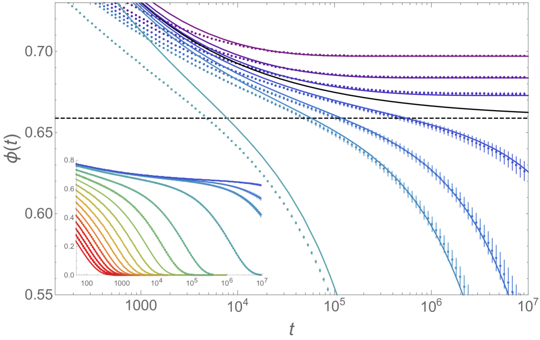
Figure 1: Double-step relaxation of the persistence in KA with $z=6$, $m=3$. Points correspond to numerical simulations on graphs with $N=64\times 10^{5}$ sites. From bottom left to top right the densities are $\rho=0.83,0.8335,0.834,0.8345,0.835,0.8355,0.8365$. Continuous lines represent the numerical solution of the MCT integral equation (1), with $\lambda$ and $\sigma$ computed analytically (we remind that $\sigma$ is a constant times $\delta\rho=\rho-\rho_{c}$)). Note that Equation (1) fix $\phi(t)$ up to a rescaling of time. We fit the timescale from the data at the critical point, where $\phi(t)\approx\phi_{plat}+(t/t_{0})^{-a}$, obtaining $t_{0}\approx 0.3$. Inset: persistence versus time for various densities ($0.7\leq\rho\leq 0.8345$).

On the BL the critical dynamics of KA is qualitatively the same as that of other KCMs, like FA. An order parameter of the problem is provided by the persistence function $\phi(t)$, counting the fraction of sites occupied by a particle that never moved up to time $t$. The ergodicity-breaking transition $\rho=\rho_{c}(z,m)$, separates a low-density (liquid) phase $\rho<\rho_{c}(z,m)$ where the persistence $\phi(t)$ relaxes to zero in the long-time limit, from a high-density (glassy) phase $\rho>\rho_{c}(z,m)$ where $\phi(t)$ reaches a non-zero plateau (see Fig. 1). This means that in the glassy phase there is a finite fractions of particles of the system that are permanently blocked. Depending on the value of the facilitation $m$, the transition at $\rho_{c}(z,m)$ is discontinuous, for $1<m<z-1$, or continuous for $m=1$. We call $\phi_{plat}(z,m)$ the plateau value of the persistence function at the critical point. As we are going to show in the next sections, the relaxation of the persistence function close to the critical point in the liquid phase is characterized by two time-scales described by MCT dynamical equations. This means that for densities close to the critical one, $\rho\lesssim\rho_{c}(z,m)$, there is a so-called $\beta$-regime corresponding to a time-scale $\tau_{\beta}$ on which the persistence is almost equal to $\phi_{plat}(z,m)$ followed by a so-called $\alpha$-regime, during which the persistence decays from $\phi_{plat}(z,m)$ to zero. Within MCT the deviations of the dynamical correlators from the plateau value in the $\beta$ regime is controlled by the following equation [5]:

$$\sigma=-\lambda\,g^{2}(t)+\frac{d}{dt}\,\int_{0}^{t}\,g(t^{\prime})\,g(t-t^{\prime})\,dt^{\prime}\ ,$$ (1)

where $\sigma$ is a linear function of $\rho-\rho_{c}$. In the liquid phase Eq. (1) implies that $g(t)$ leaves the plateau with a $-t^{b}$ law, and the model-dependent exponents $a$ and $b$ are determined by the so-called parameter exponent $\lambda$ through:

$$\lambda=\frac{\Gamma^{2}(1-a)}{\Gamma(1-2a)}=\frac{\Gamma^{2}(1+b)}{\Gamma(1+2b)}.$$ (2)

Let us introduce the “master functions” $f_{\pm}$, which are the solutions of Eq. (1) with $\sigma=\pm 1$. From Eq. (1) it follows that $g(t)$ is $O(\sqrt{|\sigma}|)$ in the $\beta$ regime and obeys the following scaling law:

$$g(t)=\sqrt{|\sigma|}\,f_{\pm}(t/\tau_{\beta}),$$ (3)

where one has to take $f_{+}$ or $f_{-}$ depending if, respectively, $\sigma$ is positive or negative. Moreover, the $\beta$ timescale, $\tau_{\beta}$, diverges with $\sigma$ from both sides as $\tau_{\beta}\propto|\sigma|^{-1/(2\,a)}$. Similarly, the time-scale of the $\alpha$ regime increases as $\tau_{\alpha}\propto|\sigma|^{-\gamma}$ with $\gamma=1/(2a)+1/(2b)$.

All of the above scaling laws have been shown to hold in FA with $g(t)\equiv\phi(t)-\phi_{plat}$ [8], where $\phi(t)$ is a persistence function analogous to the one we defined for KA. In the following, we show that the same analysis can be extended to KA, deriving an equation for the deviation of the persistence from its plateau value equivalent to (1) together with analytical expressions for the exponents $a$ and $b$ through the parameter $\lambda$.

II.2 The cavity equations for the plateau and the critical density

The plateau value of the persistence and the critical density can be computed on the BL with the cavity method, similar to the FA case. In fact, consider a reference site $i$ and one of its neighbors, which we call “root”. Based on [15], we define the “cavity” probabilities $Y,F,B$:

1. $Y(t)$ is the probability that $i$ is occupied and blocked, conditioned to the root to be occupied, up to time $t$, and it can be represented by the following diagram:

   $$Y(t)=\begin{gathered}\scalebox{0.85}{ \leavevmode\hbox to76.53pt{\vbox to72.51pt{\text{[drawing]}}} }\end{gathered}, i$$ (4)

   where the circle with dashed circumference represents a blocked site. Occupied sites are represented by filled circles. Empty sites will be represented by white circles;

2. $F(t)$ is the probability that $i$ is occupied and blocked if the root is conditioned to be empty up to time $t$. Note that the reference sites satisfying this condition is a subset of those satisfying (i). Pictorially:

   $$F(t)=\begin{gathered}\scalebox{0.85}{ \leavevmode\hbox to76.53pt{\vbox to72.51pt{\text{[drawing]}}} }\end{gathered}, i$$ (5)

3. $B(t)$ is the probability that $i$ is empty, and that it is not possible for a particle occupying the root to move to $i$ up to time $t$.

We use the notation $\lim_{t\rightarrow\infty}Y(t)=Y$, $\lim_{t\rightarrow\infty}F(t)=F$ and $\lim_{t\rightarrow\infty}B(t)=B$. The plateau value $\phi_{plat}$ of the persistence $\phi(t)$, that corresponds to the probability that a site on the graph is occupied by a blocked particle, can be easily expressed in terms of $Y$ and $B$:

$$\phi_{plat}=\rho\sum_{j=m+1}^{z}\binom{z}{j}Y^{j}(1-Y)^{z-j}+\\ +\rho\sum_{j=0}^{m}\binom{z}{j}Y^{j}B^{z-j}.$$ (6)

The cavity probabilities $Y$, $B$, and $F$ can be determined by solving a set of self-consistent equations of the following form (see Appendix A):

$$Y=\rho\,G^{(Y)}(Y,B),$$ (7)

$$F=\rho\,G^{(F)}(Y,B),$$ (8)

$$B=(1-\rho)\,G^{(B)}(F).$$ (9)

The critical values of $Y,B,F,\rho$ can be obtained by means of a stability analysis of Eqs.(7),(8),(9). For densities $\rho$ larger than the critical one $\rho>\rho_{c}$, there is a non-trivial solution of the self-consistent equations, and the fixed point is stable. In particular in this regime one finds that the eigenvalues of the Jacobian associated with the system linearized on the fixed point are all smaller than one. For $\rho=\rho_{c}$ there is a critical mode corresponding to an eigenvalue of the Jacobian equal to one. As soon as the denisity becomes smaller than $\rho_{c}$ the non-trivial fixed point destabilizes along the direction of the critical mode, and the system becomes a liquid. Therefore the critical values of $Y,B,F$ and $\rho$ are given by the solution of Eqs. (7), (9) and (8), with the addition of:

$$0=\det{\big{(}\mathds{1}-\boldsymbol{J}(Y,B,F,\rho)\big{)}},$$ (10)

where $\mathds{1}$ is the $3\times 3$ identity matrix, and $\boldsymbol{J}(Y,B,F,\rho)$ is the Jacobian matrix obtained linearizing the system of Eqs. (7), (9), (8) w.r.t. $Y,B,F$.

III Dynamical equations in the $\beta$ regime

III.1 The blocked persistences

In order to derive the equations for the dynamics of the persistence, we start with a number of definitions that have been introduced for the first time in [8] for the study of the FA. We define the blocked persistence $\phi_{b}(t)$ as the fraction of particles that have been blocked at all times less than $t$. Naturally, we have $\phi(t)\geq\phi_{b}(t)$, since a particle that is facilitated (i.e. not blocked) does not necessarily move. Note that in the infinite time limit, one has $\lim_{t\rightarrow\infty}\phi(t)=\lim_{t\rightarrow\infty}\phi_{b}(t)=\phi_{plat}$. Crucially, it is possible to argue that at large times $\delta\phi_{b}(t)\equiv\phi_{b}(t)-\phi_{plat}$ and $\delta\phi(t)\equiv\phi(t)-\phi_{plat}$ approach zero with the same leading term $(t/t_{0})^{-a}$. This is observed numerically in [8]. In App. B we present an argument to justify this equivalence in the large time limit.

Keeping in mind the definitions given in Sec. II.2, we note that for a particle $i$ to be blocked at a certain time, it must have a blocking set, i.e. a set composed by either: a) at least $m+1$ neighboring occupied sites, or b) at least $z-m$ empty neighboring sites that cannot be occupied by $i$, and $z-j$ neighboring occupied sites. We define the zero-switch blocked persistence $\phi_{b}^{(0)}(t)$ as the fraction of particles that have been blocked up to time $t$ because their blocking set has remained the same throughout the interval $(0,t)$. This zero-switch persistence reads:

$$\phi_{b}^{(0)}(t)=\rho\sum_{j=m+1}^{z}\,\binom{z}{j}\,Y^{j}(t)\,(1-Y(t))^{z-j}+\\ +\rho\sum_{j=0}^{m}\binom{z}{j}\,Y^{j}(t)\,B^{z-j}(t).$$ (11)

For $z=4,m=2$ the possible contributions entering Eq. (11) can be represented graphically as:

$$\begin{split}\phi_{b}^{(0)}(t)=&\begin{gathered}\scalebox{0.5}{ \leavevmode\hbox to73.23pt{\vbox to73.23pt{\text{[drawing]}}} }\end{gathered}\quad+\quad\begin{gathered}\scalebox{0.5}{ \leavevmode\hbox to73.23pt{\vbox to73.23pt{\text{[drawing]}}} }\end{gathered}+\\ &+\begin{gathered}\scalebox{0.5}{ \leavevmode\hbox to76.03pt{\vbox to76.03pt{\text{[drawing]}}} }\end{gathered}+\begin{gathered}\scalebox{0.5}{ \leavevmode\hbox to76.03pt{\vbox to76.03pt{\text{[drawing]}}} }\end{gathered}+\begin{gathered}\scalebox{0.5}{ \leavevmode\hbox to76.03pt{\vbox to74.63pt{\text{[drawing]}}} }\end{gathered}\end{split}$$ (12)

where the full lines represent the neighbors of the blocked particle (circle) which have always remained occupied at all times less than $t$, the double lines represent empty neighbors that cannot be occupied, and the dashed line represents an unconditioned neighbor. Therefore, the first term in Eq. (11), which takes into account the case in which there are at least $m+1$ occupied neighbors, is represented by the first two diagrams. The second in Eq. (11), taking into account the case in which there are at least $z-m$ empty neighbors that cannot be occupied, and the remaining neighbors are occupied, is represented by the remaining three diagrams. Note that taking the infinite-time limit, Eq. (11) reduces to the equation for the plateau value of the persistence (Eq. (6)). We also define the one-switch blocked persistence $\phi_{b}^{(1)}(t)$ as the the fraction of blocked particles s.t. their blocking set is composed by $m$ neighbors that have been always occupied, and a so-called switching couple of neighbors. A switching couple is composed by a first neighboring site which has been occupied up to some time $t^{\prime}$, and a second neighbor, that has been occupied in $(t^{\prime\prime},t)$, where $0<t^{\prime\prime}<t^{\prime}<t$. Note that $t^{\prime\prime}>0$, otherwise this contribution is already taken into account by $\phi_{b}^{(0)}(t)$. For example in the case $z=4,m=2$, the term with $t^{\prime\prime}=0$ is given by the second diagram in Eq. (12). Also $\phi_{b}^{(1)}(t)$ can be represented graphically. For $z=4,m=2$ we have:

$$\phi_{b}^{(1)}(t)=\begin{gathered}\scalebox{0.5}{ \leavevmode\hbox to73.23pt{\vbox to73.23pt{\text{[drawing]}}} }\end{gathered}.$$ (13)

The top lines in the diagram (13) represent the switching couple of neighbors: the top right line corresponds to the neighbor which is occupied up to time $t^{\prime}$, and the top left line the neighbor which is occupied between $t^{\prime\prime}$ and $t$.

Following [8], one-switch blocked persistence can also be expressed in terms of cavity persistence. Let’s call $i_{1}$ and $i_{2}$ the switching couple of neighbors of an occupied site $i_{0}$ counted by $\phi_{b}^{(1)}(t)$. Recalling the definition of $Y(t)$, it follows that the probability that $i_{1}$ was occupied up to $t^{\prime}$, and that it frees between $t^{\prime}$ and $t^{\prime}+dt^{\prime}$, is given by $-(dY(t^{\prime})/dt^{\prime})dt^{\prime}$. The total probability that $i_{2}$ is occupied between time $t^{\prime\prime}$ and $t$ with $0<t^{\prime\prime}<t^{\prime}$ can be computed invoking the reversibility of the dynamics: it is equal to the probability that starting at equilibrium at time $t$, and moving backward in time the site is occupied up to time $t-t^{\prime}$ but not up to time $t$, leading to a factor $Y(t-t^{\prime})-Y(t)$. As already discussed, we have to subtract $Y(t)$ because the case $t^{\prime}=0$ (and then $t^{\prime\prime}=0$) leads to a contribution which is already taken into account by the zero-switch persistence. At this point: i) multiplying by a combinatorial factor counting all possible switching couples of neighbors; ii) multiplying by the probability $\rho$ that $i_{0}$ is occupied in the initial condition; iii) multiplying by the probability $Y^{m}(t)$ that the neighbors of $i_{0}$ not belonging to the switching couple are occupied at all times less than $t$; iv) integrating over $t^{\prime}$, we obtain the following formula:

$$\phi_{b}^{(1)}(t)=\rho\,\binom{z}{m}\,(z-m)\,(z-m-1)\,Y(t)^{m}\times\\ \times(1-Y(t))^{z-m-2}\,\int_{0}^{t}dt^{\prime}\frac{dY(t^{\prime})}{dt^{\prime}}(Y(t-t^{\prime})-Y(t)).$$ (14)

In the next section, we use the quantities defined here to write a closed equation for $\phi(t)$.

III.2 The critical hierarchy

$z$	$m$	$\rho_{c}$	$\phi_{plat}$	$\lambda$	$a$	$b$
4	2	0.888793	0.788605	0.673328	0.337761	0.685369
5	2	0.724831	0.32489	0.716273	0.320017	0.613758
5	3	0.948964	0.942315	0.649708	0.346793	0.725438
6	2	0.602788	0.11982	0.734512	0.311883	0.583671
6	3	0.834769	0.65877	0.701751	0.326226	0.637831
6	4	0.970598	0.969832	0.643283	0.34917	0.736444
7	2	0.513688	0.0477438	0.744701	0.307162	0.566909
7	3	0.730949	0.523061	0.723766	0.316723	0.601382
7	4	0.886856	0.777713	0.702238	0.326021	0.637021
7	5	0.980847	0.954341	0.643002	0.349274	0.736926
8	2	0.446765	0.182959	0.75112	0.304117	0.556359
8	3	0.645919	0.430747	0.737636	0.31045	0.578529
8	4	0.80069	0.655943	0.722238	0.3174	0.603903
8	5	0.916342	0.843202	0.712058	0.321843	0.620734
8	6	0.986518	0.969399	0.645149	0.348483	0.733243

Table 1: Dynamical parameters of the KA model on the Bethe lattice with connectivity $z$ and facilitation $m$.

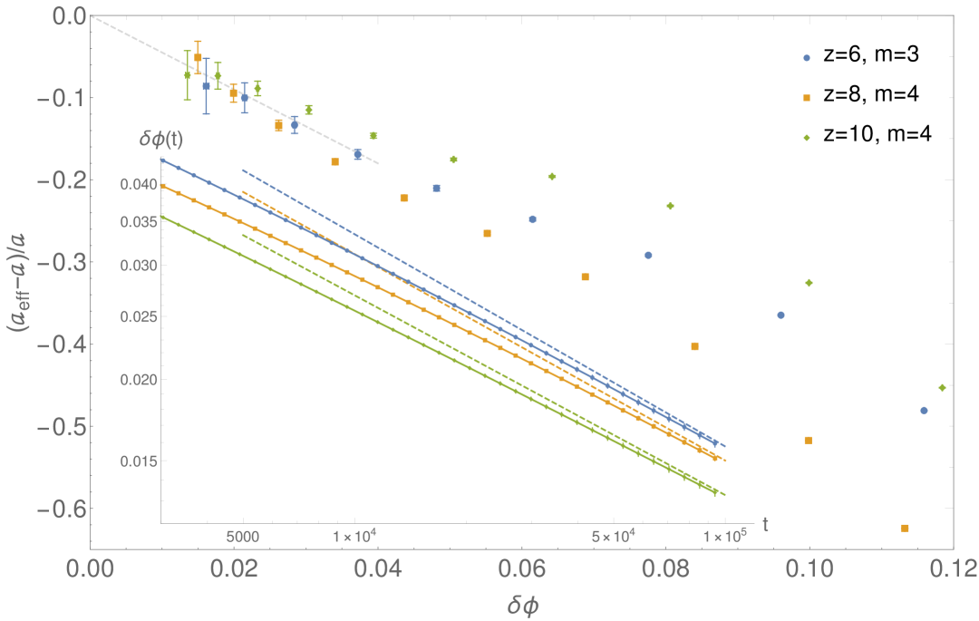
Figure 2: Parametric plot of the relative shift of the effective exponent $a_{eff}$ with respect to the analytical prediction $a$ vs. the shift $\delta\phi$ from the plateau. From bottom right to top right: $z=8$ $m=4$, $z=6$ $m=3$ and $z=10$ $m=4$. The dashed line is a guide for the eye. Inset: distance of the persistence from the plateau value vs $t$. From top right to bottom right: $z=8$ $m=4$, $z=6$ $m=3$ and $z=10$ $m=4$. Continuous lines correspond to curves of proportional to $t^{-a_{z,m}}$, where $a_{z,m}$ are predicted analytically (see Table 1). Each point is obtained by performing numerical simulations at different sizes ($10^{5}<N<10^{6}$), and then extrapolating to infinite volume.

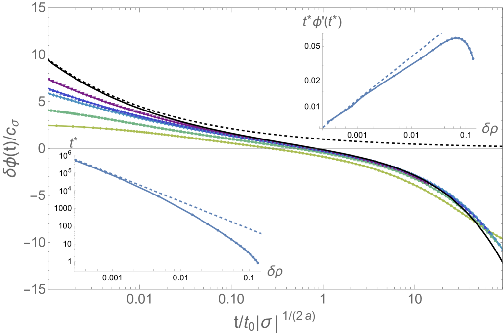
Figure 3: Scaling laws in the $\beta$-regime for $z=6$ and $m=3$. The continuous black line represents the master function $f_{-}$. The dashed line is the critical shift of the persistence $t^{-a}$. The other curves are numerical estimates of the shifted rescaled persistence. From bottom left to top left $\rho=0.82,0.83,0.8335,0.834,0.8345$. The top right inset tests Eq. (29). The dashed line represents $\hat{t}\,f_{-}(\hat{t})\,\sqrt{|\sigma|}$. The bottom left inset tests Eq. (28). The dashed line represents $t_{0}\,\hat{t}\,\sigma^{-\frac{1}{2a}}$, with $t_{0}\approx 0.3$ fitted from the data at the critical point and $a$ given by our analytical estimate. Numerical simulations are obtained on graphs with $N=64\times 10^{5}$ sites.

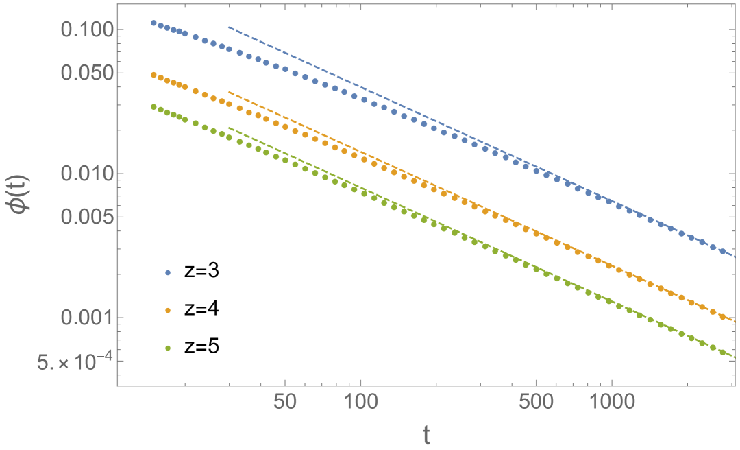
Figure 4: Persistence in KA continuous models ($m=1$). From top to bottom: $z=3,4,5$. The dashed lines correspond to $C_{z}t^{-2a}$, where $a=0.395263$ is the analytical prediction, and $C_{3}\approx 1.52$, $C_{4}\approx 0.54$ and $C_{5}\approx 0.305$. Numerical data correspond to the average of $20$ samples of size $N=64\times 10^{6}$.

The blocked cavity persistence can be always written as as sum of zero-switch and one-switch persistences, plus an error $\Delta\phi_{b}(t)>0$ that counts all contributions to $\phi_{b}(t)$ other than $\phi_{b}^{(0)}(t)$ and $\phi_{b}^{(1)}(t)$:

$$\phi_{b}(t)=\phi_{b}^{(0)}(t)+\phi_{b}^{(1)}(t)+\Delta\phi_{b}(t)\ .$$ (15)

In FA [8] it is shown that in the $\beta$-regime a hierarchy between the different contributions emerges:

$$1\gg\phi_{b}^{(0)}(t)-\phi_{plat}\gg\phi_{b}^{(1)}(t)\gg\Delta\phi_{b}(t)\ \ \ t\gg 1\ .$$ (16)

In particular, it is found that $\phi_{b}^{(0)}(t)-\phi_{plat}\approx t^{-a}$, $\phi_{b}^{(1)}(t)\approx t^{-2a}$, $\Delta\phi_{b}(t)\approx t^{-3a}$ for some $a>0$ predicted by the theory. It is also shown that in order to compute the persistence $\phi_{b}(t)$ in the $\beta$-regime close to the critical point, it is sufficient to truncate (15) at the one-switch order:

$$\phi_{b}(t)\approx\phi_{b}^{(0)}(t)+\phi_{b}^{(1)}(t).$$ (17)

Let us assume the validity of the critical hierarchy (16). We are going to check the consistency of (16) a posteriori, by comparing the predictions obtained under this assumption, e.g. the critical exponent $a$, with numerical simulations. Under (16), the one-switch contribution $\phi_{b}^{(1)}(t)$ can be interpreted as a correction to the first term of (11), that corresponds to the case in which the occupied site is blocked because it has more than $m$ occupied neighbors. Note that we ignored one-switch corrections to the second term of (11), taking into account the case in which the occupied site is blocked because all its neighbors are blocked. This is the case because all the neighbors must be blocked at all times, and the probability that a site switches from being blocked and occupied to being blocked and empty is negligible. From Eq. (17), to compute the critical behavior of $\phi(t)$, we need to analyze the cavity persistences, which, as shown in Sec. III, are used to express both $\phi_{b}^{(0)}(t)$ and $\phi_{b}^{(1)}(t)$. Indeed, as we have seen in Sec. III, both $\phi_{b}^{(0)}(t)$ and $\phi_{b}^{(1)}(t)$ are expressed in terms of the cavity persistences. At this point the strategy is to also express $Y(t),B(t),F(t)$ in terms of blocked persistences, and to truncate the blocked persistences at the one-switch term, which is assumed to be exact in the $\beta$-regime close to the critical point. Therefore, we have:

$$\delta Y(t)\approx\delta Y_{b}^{(0)}(t)+Y_{b}^{(1)}(t)$$ (18)

$$\delta B(t)\approx\delta B_{b}^{(0)}(t)+B_{b}^{(1)}(t)$$ (19)

$$\delta F(t)\approx\delta F_{b}^{(0)}(t)+F_{b}^{(1)}(t),$$ (20)

where “$\delta$” in front of a persistence means the persistence minus its plateau value. We use the following vectorial notation to write Eqs. (18), (19) and (20):

$$\boldsymbol{\delta\hat{\phi}}(t)\approx\boldsymbol{\delta\hat{\phi}}_{b}^{(0)}(t)+\boldsymbol{\hat{\phi}}_{b}^{(1)}(t),$$ (21)

where $\boldsymbol{\delta\hat{\phi}}_{b}^{(0)}(t)=\big{(}\delta Y_{b}^{(0)}(t),\delta B_{b}^{(0)}(t),\delta F_{b}^{(0)}(t)\big{)}$, and $\boldsymbol{\delta\hat{\phi}}(t)=\big{(}\delta Y(t),\delta B(t),\delta F(t)\big{)}$. The one-switch terms $\boldsymbol{\hat{\phi}}_{b}^{(1)}(t)$ can be computed repeating the arguments of Sec. III.1 (see Eq. 14). The complete expressions are written in App. C. The zero-switch blocked cavity persistences are exactly given by:

$$Y_{b}^{(0)}(t)=\rho\,G^{(Y)}\big{(}Y(t),B(t)\big{)},$$ (22)

$$B_{b}^{(0)}(t)=(1-\rho)\,G^{(B)}\big{(}F(t)\big{)},$$ (23)

$$F_{b}^{(0)}(t)=\rho\,G^{(F)}\big{(}Y(t),B(t)\big{)},$$ (24)

to be compared with Eqs. (7), (9) and (8). Close to the critical density $\rho_{c}$, i.e. for small $\delta\rho=\rho-\rho_{c}$, and on the time-scale $\tau_{\beta}$ of the $\beta$-regime, we can expand Eqs. (22), (23) and (24), recalling that the cavity peristences are close to their plateau values. In this way, we obtain an expression of the form:

$$\boldsymbol{\delta\hat{\phi}}_{b}^{(0)}(t)\approx\delta\rho\,\boldsymbol{\xi}+\boldsymbol{J}_{crit}\,\boldsymbol{\delta\hat{\phi}}(t)+\frac{1}{2}\boldsymbol{\delta\hat{\phi}}^{T}(t)\boldsymbol{H}^{(Y)}_{crit}\boldsymbol{\delta\hat{\phi}}(t)+\frac{1}{2}\boldsymbol{\delta\hat{\phi}}^{T}(t)\boldsymbol{H}^{(B)}_{crit}\boldsymbol{\delta\hat{\phi}}(t)+\frac{1}{2}\boldsymbol{\delta\hat{\phi}}^{T}(t)\boldsymbol{H}^{(F)}_{crit}\boldsymbol{\delta\hat{\phi}}(t),$$ (25)

where: i) $\boldsymbol{J}_{crit}$ is the (non-symmetric) Jacobian associated with the linearized system computed at $\rho=\rho_{c}$ and on the plateau values of the cavity persistences at the critical point; ii) $\boldsymbol{\xi}=\big{(}G^{(Y)}_{crit},-G^{(B)}_{crit},G^{(F)}_{crit}\big{)}$, and $G^{(Y)}_{crit},G^{(B)}_{crit},G^{(F)}_{crit}$ are the functions $G^{(Y)},G^{(B)},G^{(F)}$ computed on the plateau values of the cavity persistences at the critical point; iii) $\boldsymbol{H}_{crit}^{(Y)},\boldsymbol{H}_{crit}^{(B)}$ and $\boldsymbol{H}_{crit}^{(F)}$ are the matrices of second derivatives of, respectively, $\rho_{c}\,G^{(Y)},(1-\rho_{c})\,G^{(B)}$ and $\rho_{c}\,G^{(F)}$ w.r.t. the cavity persistences, computed on the plateau values of the cavity persistences at the critical point. The Jacobian $\boldsymbol{J}_{crit}$ has a critical eigenvalue equal to one (see Eq. (10)). We call, respectively, $\boldsymbol{v}^{r}$ and $\boldsymbol{v}^{l}$ the corresponding right and left critical eigenvectors. The dynamics in the $\beta$-regime is determined by the projection of the cavity persistences vector on the critical mode, since the other directions correspond to eigenvalues smaller than one, that imply an exponentially fast relaxation. For this reason in the $\beta$-regime we write

$$\boldsymbol{\delta\hat{\phi}}(t)\approx g(t)\,\boldsymbol{v}^{r},$$ (26)

and we are interested in the projection of Eqs. (21) and (25) on $\boldsymbol{v}^{l}$. Like in FA (see [8]), the linear term in $g(t)$ cancels out with the LHS of the projection of Eq. (21), and we have to consider the $g(t)^{2}$ contributions coming both from the projection of (25) and from the one-switch terms. This yields a quadratic equation for $g(t)$ in the form of (1), where $\sigma=A(\rho-\rho_{c})$, and both $A$ and $\lambda$ are expressed as functions of $z$ and $m$, with explicit formulas provided in App. C. At this point going back to the persistence $\phi(t)$, we have that in the $\beta$-regime, and for $1<m<z-1$ (discontinuous transitions)

$$\delta\phi(t)\propto g(t),$$ (27)

namely the critical behavior of $\phi(t)$ is the same of that of the cavity persistences, like for FA in the case of discontinuous transitions. Eq. (27) can be simply found substituting $Y+\delta Y(t)$ and $B+\delta B(t)$ in Eq. (11), expanding at first order, and noting (see Eq. (26)) that $\delta Y(t),\delta B(t)\propto g(t)$. Therefore also $\delta\phi(t)$ satisfies equation (1) with the same value of $\lambda$. The analytical formula for $\lambda$ provided in App. C allows us to determine the critical exponents of the $\beta$-regime using Eq. (2). In table 1 we display these critical exponents for all non-trivial values of $m$ up to $z=8$, excluded the cases with $m=1$, which correspond to continuous transitions (see Sec. III.3). In Fig. 2 we study the effective exponent $a_{eff}\equiv-d\ln\delta\phi/d\ln t$, that converges to the actual exponent $a$ at large times (small values of $\delta\phi$). In figure 3 we study the scaling laws of the $\beta$-regime, corresponding to time-scales where $\phi(t)$ remains close to the plateau value. In order to do so, we consider for densities $\rho\lesssim\rho_{c}$ the time $t^{*}$ at which $\delta\phi(t^{*})=0$, which can be measured in numerical experiments. Starting from Eq. (3), if $\hat{t}$ satisfies $f_{-}(\hat{t})=0$, then

$$t^{*}=\hat{t}\,\tau_{\beta}=\hat{t}\,t_{0}\,\sigma^{-\frac{1}{2a}},$$ (28)

and

$$t^{*}\,\delta\phi^{\prime}(t^{*})=\hat{t}\,f_{-}(\hat{t})\,\sqrt{|\sigma|},$$ (29)

where $t_{0}$ is the microscopic time-scale that has to be fitted from numerical data. In Fig. 3 we test (28), (29), and we compare the master function $f_{-}(t)$, obtained solving numerically Eq. (1) with $\sigma=-1$, with the numerical estimates of the persistence.

III.3 Continuous Models

For $m=1$, the transition is continuous and occurs at $\rho_{c}=1/(z-1)$. In this case, the equations for $Y_{b}^{(0)}(t)$ and $Y_{b}^{(1)}(t)$ can be closed on $Y(t)$ at criticality. This fact simplifies the analysis of the previous section. In App. D we show that for continuous transitions, independently of the value of the connectivity, $Y(t)$ decays as $t^{-a}$ with $\lambda=1/2\,\rightarrow\ a=0.395263$, and $\phi(t)$ is quadratic in $Y(t)$, implying that its dynamic exponent is doubled: $\phi(t)\,\approx\,z\,Y^{2}(t)/2\,\propto 1/t^{2a}$. The same holds for continuous FA [8]. In Fig. 4 we show the persistence for connectivity $z=3,4,5$, confirming the prediction that the exponent does not depend on $z$.

III.4 The $\alpha$ regime

The dynamical hierarchy leading to equation (1) is only valid in the $\beta$ regime, corresponding to time-scales where $\phi(t)$ remains close to the plateau value. Nonetheless from the equation itself one can deduce, as we mentioned below Eq. (1), not only the scaling law of the $\beta$ regime $\tau_{\beta}\propto|\sigma|^{-1/(2\,a)}$ but also the time-scale of the $\alpha$ regime $\tau_{\alpha}$. The scaling function (3) implies that in the liquid phase $g(t)$ leaves the plateau with a power law behavior $-t^{b}$. The $\alpha$ regime can be identified as the time when $g(t)$ is no longer small and becomes $O(1)$. This occurs when $(\tau_{\alpha}/\tau_{\beta})^{b}\sqrt{|\sigma|}=O(1)$ leading to $\tau_{\alpha}\propto|\sigma|^{-\gamma}$ with $\gamma=1/(2a)+1/(2b)$. In the $\alpha$ regime it can be argued that the following scaling law is obeyed:

$$\phi(t)=C_{\alpha}(t/\tau_{\alpha})$$ (30)

where the function $C_{\alpha}(x)$ is model-dependent at variance with the function $f_{\pm}(x)$ that depends only on $\lambda$. See Figure 5 for a numerical check of the scaling $\tau_{\alpha}\propto|\sigma|^{-\gamma}$ in the case of KA, and [10] in the case of FA.

The scaling function $C_{\alpha}(x)$ cannot be determined solely from Eq. (1). This equation is quadratic in $g(t)=\delta\phi(t)$ and therefore is accurate as long as $\delta\phi$ is close to the plateau, i.e. on the time scale $\tau_{\beta}$. Instead in the $\alpha$ regime, by definition, $\delta\phi$ is $O(1)$ because the system leaves the plateau. As a consequence, terms of order $\delta\phi^{3}(t)$ and higher become important. These terms do not change the scaling laws of the critical exponents, i.e. $a$, $b$ and $\gamma$, but determine the model-dependent scaling function $C_{\alpha}(x)$. A non-perturbative approximation to the scaling function can be obtained closing Eq. (21) with the complete expressions of $\boldsymbol{\hat{\phi}}_{b}^{(0)}(t)$ (see Eqs. (22), (23), (24)) and $\hat{\phi}_{b}^{(1)}(t)$ (see Eqs. (40), (41) and (42)). Note that this is different from what we were doing in the $\beta$ regime, where the expression for $\boldsymbol{\hat{\phi}}_{b}^{(0)}(t)$ is expanded close to its plateau value (see Eq. (25)). This approximation yields a solution for $C_{\alpha}(t)$ that goes to zero at large times because Eqs. (22), (23) and (24) imply that $\hat{\phi}_{b}^{(0)}(t)=0$ if $\hat{\phi}_{b}(t)=0$, and $\hat{\phi}_{b}^{(1)}(t)$ tends to zero if $\hat{\phi}_{b}(t)=0$ tends to zero. We show this solution in Fig. 5. Despite the fact that it satisfies $\hat{\phi}_{b}(\infty)=0$, it is not particularly accurate.

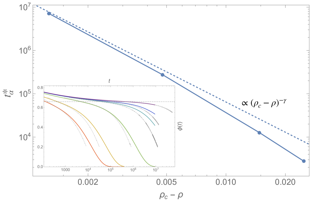
Figure 5: Estimate of the $\alpha$ time-scale $\tau_{\alpha}$, obtained computing the time $t^{*}_{\alpha}$ at which $\phi(t)=C$ as a function of $\rho_{c}-\rho$, where $C<\phi_{plat}$ is a constant. Here we choose $C=0.45$. If the scaling-law (30) is verified, then $t^{*}_{\alpha}\propto\tau_{\alpha}$. The data correspond to the case $z=6,m=3$, where the analytical computation of the critical exponents (see Table 1) gives $\gamma=2.31659\dots$. Inset: comparison between the persistence derived from the approximate scaling function of the $\alpha$-regime (dotted gray lines), and numerical data (continuous lines) for $\rho=0.81,0.82,0.83,0.8335,0.834,0.8345$. The scaling function, computed from the non-perturbative approximation obtained closing Eq. (21) with the complete expressions of $\boldsymbol{\hat{\phi}}_{b}^{(0)}(t)$ and $\boldsymbol{\hat{\phi}}_{b}^{(1)}(t)$ (see section III.4), reproduces qualitatively the behavior of the data. Numerical simulations are obtained on graphs with $N=64\times 10^{5}$ sites.

IV Conclusions

In this work, we presented the analytical solution of the dynamics of the Kob-Andersen model on the Bethe lattice in the critical regime. Similarly to other models of supercooled liquids, the dynamics near the critical point exhibits a two-stage relaxation behavior, captured by the persistence function, which is an order parameter for the problem. Extending the combinatorial argument introduced in [8] for the Fredrickson-Andersen model, we have shown that the persistence function obeys the very same critical equation of MCT. By means of numerical experiments, we have verified that the model displays indeed the whole MCT critical phenomenology, notably: i) the power-law divergences of the $\beta$ and $\alpha$ times scales as $\tau_{\beta}\propto|\delta\rho|^{-\frac{1}{2\,a}}$ and $\tau_{\alpha}\propto|\delta\rho|^{-\gamma}$, ii) $1/t^{a}$ approach to the plateau at the critical point and iii) the scaling law $\phi(t)-\phi_{plat}\propto|\delta\rho|^{1/2}\,f_{\pm}(t/\tau_{\beta})$ in the $\beta$ regime. Furthermore the numerical data are in excellent quantitative agreement with our analytical predictions for the critical exponents. The theory has been also validated in the context of continuous transitions.

Appendix A Cavity Equations for $Y,B$ and $F$

Following [15], we write the fixed-point equations for the plateau values of the cavity persistences:

$$Y=\rho\,\left(\sum_{j=m}^{z-1}\binom{z-1}{j}Y^{j}(1-Y)^{z-1-j}+\sum_{j=0}^{m-1}\binom{z-1}{j}Y^{j}B^{z-1-j}\right)\equiv\rho\,G^{(Y)}(Y,B),$$ (31)

$$F=\rho\left(\sum_{j=m+1}^{z-1}\binom{z-1}{j}Y^{j}(1-Y)^{z-1-j}+\sum_{j=0}^{m}\binom{z-1}{j}Y^{j}B^{z-1-j}\right)\equiv\rho\,G^{(F)}(Y,B).$$ (32)

$$B=(1-\rho)\sum_{j=m+1}^{z-1}\binom{z-1}{j}F^{j}(1-F)^{z-1-j}\equiv(1-\rho)\,G^{(B)}(F),$$ (33)

Based on the definitions of $B,F,Y$ given in Sec. II.2, we can write the plateau value of the persistence as follows:

$$\phi=\rho\sum_{j=m+1}^{z}\binom{z}{j}Y^{j}(1-Y)^{z-j}+\\ +\rho\sum_{j=0}^{m}\binom{z}{j}Y^{j}B^{z-j}.$$ (34)

In Fig. 6 we show the plateau value of $B,F,Y$ as a function of the density $\rho$ for $z=6,m=3$, computed solving the self-consistency Eqs. (31), (32) and (33). In Fig. 7 we show the plateau value of the persistence as a function of $\rho$ for $z=6,m=3$.

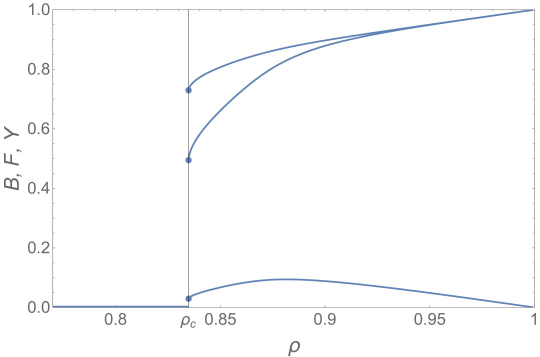
Figure 6: Plateau values of the cavity persistences as a function of the density $\rho$, for $z=6$, $m=3$. From top to bottom $Y,F,B$.

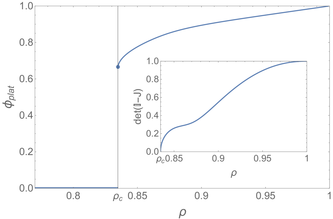
Figure 7: Plateau value of the persistence as a function of the density $\rho$, for $z=6,m=3$. Inset: value of $\det{\big{(}\mathds{1}-\boldsymbol{J}(Y(\rho),B(\rho),F(\rho),\rho)\big{)}}$ as a function of $\rho$, where $Y(\rho),B(\rho),F(\rho)$ are the respective non-trivial solutions of the cavity equations. For $\rho\rightarrow\rho_{c}^{+}$ the determinant goes to zero, as a consequence of the destabilization of the non-trivial fixed point.

Appendix B Asymptotic Equivalence between persistence and blocked persistence

The argument is as follows. Let us start by noticing that the higher the number of times a particle is facilitated, the lower the probability that it does not move from its initial position. Now, due to the reversibility of the dynamics, if the particle was facilitated at some distant time in the past with probability one, it must have been facilitated many times at later times, leading to a vanishing probability that it did not move. In other words we expect that once a particle becomes facilitated at time $t$, it will move with probability one after a finite time $t_{sw}$ that is short on the time scale of the critical dynamics. Therefore the difference between the persistence $\phi(t)$ at time $t$ and the blocked persistence $\phi_{b}(t)$ is controlled by the fraction $\delta_{sw}(t)$ of the number of particles that become facilitated between times $t$ and $t+t_{sw}$, because these particle will typically start to move after $t_{sw}$. In formulas:

$$\phi(t)\approx\phi_{b}(t)+\delta_{sw}(t),$$ (35)

where $\delta_{sw}$ is just given by:

$$\delta_{sw}=\phi_{b}(t)-\phi_{b}(t+t_{sw})\approx-t_{sw}\frac{d\phi_{b}(t)}{dt}.$$ (36)

Using the fact that in the $\beta$-regime $\phi(t)-\phi_{plat}\approx 1/t^{a}$, Eq. (35) implies that for large times also $\phi_{b}(t)-\phi_{plat}\approx 1/t^{a}$, and in particular that their difference is $O(1/t^{a+1})$. As we are going to see in the following, terms $O(1/t^{a+1})$ can be neglected for the characterization of the dynamics at the leading order.

Appendix C The dynamical equations

As discussed in the main text, the critical dynamics is determined by the projection of the cavity persistences on the critical mode of the Jacobian $\boldsymbol{J}_{crit}$. For this reason we write:

$$\boldsymbol{\delta\hat{\phi}}(t)\approx g(t)\,\boldsymbol{v}^{r},$$ (37)

where $\boldsymbol{v}^{r}$ and $\boldsymbol{v}^{l}$ are, respectively, the right and the left critical eigenvectors. Let us denote the coordinates of $\boldsymbol{v}^{r}$ and $\boldsymbol{v}^{l}$, respectively, as $\boldsymbol{v}^{r}=(v^{r}_{Y},v^{r}_{B},v^{r}_{F})$ and $\boldsymbol{v}^{r}=(v^{l}_{Y},v^{l}_{B},v^{l}_{F})$. Projecting (25) on $\boldsymbol{v}^{l}$ we find

$$\boldsymbol{v}^{l}\cdot\boldsymbol{\delta\hat{\phi}}_{b}^{(0)}(t)=g(t)+\delta\rho\,\boldsymbol{v}^{l}\cdot\boldsymbol{\xi}+C_{z,m}g(t)^{2}+\dots,$$ (38)

where

$$C_{z,m}=\frac{v^{l}_{Y}}{2}(\boldsymbol{v}^{r})^{T}\boldsymbol{H}_{crit}^{(Y)}\boldsymbol{v}^{r}+\frac{v^{l}_{B}}{2}(\boldsymbol{v}^{r})^{T}\boldsymbol{H}_{crit}^{(B)}\boldsymbol{v}^{r}+\\ +\frac{v^{l}_{F}}{2}(\boldsymbol{v}^{r})^{T}\boldsymbol{H}_{crit}^{(F)}\boldsymbol{v}^{r}.$$ (39)

Following the same arguments of section III, we can write the one-switch blocked cavity persistences in the following way:

$$Y_{b}^{(1)}(t)=-\rho\,\binom{z-1}{m-1}(z-m)(z-m-1)Y(t)^{m-1}(1-Y(t))^{z-m-2}\int_{0}^{t}ds\frac{dY(s)}{ds}(Y(t-s)-Y(t))$$ (40)

$$F_{b}^{(1)}(t)=-\rho\,\binom{z-1}{m}(z-1-m)(z-2-m)Y(t)^{m}(1-Y(t))^{z-m-3}\int_{0}^{t}ds\frac{dY(s)}{ds}(Y(t-s)-Y(t)).$$ (41)

$$B_{b}^{(1)}(t)=-(1-\rho)\,\binom{z-1}{m}(z-1-m)(z-2-m)F(t)^{m}(1-F(t))^{z-3-m}\int_{0}^{t}ds\frac{dF(s)}{ds}(F(t-s)-F(t))$$ (42)

Using Eq. (37), and expanding at the leading order in $g(t)$, we have

$$\boldsymbol{v}^{l}\cdot\boldsymbol{\hat{\phi}}^{(1)}_{b}=D_{z,m}\,\int_{0}^{t}ds\frac{dg(s)}{ds}\big{(}g(t-s)-g(t)\big{)},$$ (43)

where

$$\begin{split}D_{z,m}=&-\rho_{c}\,\binom{z-1}{m-1}\,(z-m)(z-m-1)\,Y^{m-1}\,(1-Y)^{z-m-2}\,v_{Y}^{l}\,(v_{Y}^{r})^{2}+\\ &-(1-\rho_{c})\,\binom{z-1}{m}\,(z-1-m)(z-2-m)\,F^{m}\,(1-F)^{z-3-m}\,v_{B}^{l}\,(v_{F}^{r})^{2}+\\ &-\rho_{c}\,\binom{z-1}{m}\,(z-1-m)(z-2-m)\,Y^{m}\,(1-Y)^{z-m-3}\,v_{F}^{l}\,(v_{Y}^{r})^{2}.\end{split}$$ (44)

Therefore substituting Eqs. (43) and (38) into the projection of (21) on $\boldsymbol{v}^{l}$, and integrating by parts, we get:

$$-\frac{\boldsymbol{v}^{l}\cdot\xi}{D_{z,m}}\,\delta\rho=-\left(1-\frac{C_{z,m}}{D_{z,m}}\right)g(t)^{2}+\frac{d}{dt}\int_{0}^{t}ds\,g(s)\,g(t-s),$$ (45)

that is written in the MCT form (see Eq. (1)), implying that:

$$\lambda=1-\frac{C_{z,m}}{D_{z,m}},\quad\sigma=-\frac{\boldsymbol{v}^{l}\cdot\boldsymbol{\xi}}{D_{z,m}}\,\delta\rho.$$ (46)

Appendix D Continuous Transitions

For $m=1$ the transition is continuous, and the analysis of section III simplifies, since to discuss the critical dynamics, the only relevant cavity persistence is $Y(t)$. Recall that in the continuous case $Y(t)$ tends to zero for large times. Expanding (22) for small $Y(t)$ up to the second order at the critical point $\rho_{c}=1/(z-1)$, we find:

$$Y_{b}^{(0)}(t)=Y(t)-\frac{1}{2}(z-2)Y(t)^{2},$$ (47)

and equation (40) becomes

$$Y_{b}^{(1)}(t)=-(z-2)\int_{0}^{t}ds\frac{dY(s)}{ds}(Y(t-s)-Y(t)).$$ (48)

Therefore, using

$$Y(t)=Y_{b}^{(0)}(t)+Y_{b}^{(1)}(t),$$ (49)

we find $\lambda=1/2$, independently of $z$. Now consider the persistence $\phi(t)$. The zero-switch blocked persistence $\phi_{b}^{(0)}(t)$ is given by:

$$\phi_{b}^{(0)}(t)=\rho\left(\sum_{j=m+1}^{z}\binom{z}{j}Y(t)^{j}(1-Y(t))^{z-j}+\sum_{j=0}^{m}\binom{z}{j}Y(t)^{j}B(t)^{z-j}\right).$$ (50)

For $m=1$, at $\rho_{c}=1/(z-1)$, and close to the plateau, we have $\phi_{b}^{(0)}(t)\approx\frac{z}{2}\,Y(t)^{2}$, and the one-switch blocked persistence $\phi_{b}^{(1)}(t)$ (see the main text) is $O(Y(t)^{3})$, therefore

$$\phi(t)\approx\frac{z}{2}\,Y(t)^{2}.$$ (51)

References

- Kirkpatrick et al. [1989] T. R. Kirkpatrick, D. Thirumalai, and P. G. Wolynes, Scaling concepts for the dynamics of viscous liquids near an ideal glassy state, Physical Review A 40, 1045 (1989).
- Thirumalai and Kirkpatrick [1988] D. Thirumalai and T. Kirkpatrick, Mean-field potts glass model: Initial-condition effects on dynamics and properties of metastable states, Physical Review B 38, 4881 (1988).
- Kirkpatrick and Thirumalai [1989] T. Kirkpatrick and D. Thirumalai, Random solutions from a regular density functional hamiltonian: a static and dynamical theory for the structural glass transition, Journal of Physics A: Mathematical and General 22, L149 (1989).
- Charbonneau et al. [2017] P. Charbonneau, J. Kurchan, G. Parisi, P. Urbani, and F. Zamponi, Glass and jamming transitions: From exact results to finite-dimensional descriptions, Annual Review of Condensed Matter Physics 8, 265 (2017).
- Götze [2008] W. Götze, Complex dynamics of glass-forming liquids: A mode-coupling theory, Vol. 143 (Oxford University Press, USA, 2008) pp. 304–436.
- Ritort and Sollich [2003] F. Ritort and P. Sollich, Glassy dynamics of kinetically constrained models, Advances in physics 52, 219 (2003).
- Garrahan et al. [2011] J. P. Garrahan, P. Sollich, and C. Toninelli, Kinetically constrained models, Dynamical heterogeneities in glasses, colloids, and granular media 150, 111 (2011).
- Perrupato and Rizzo [2025] G. Perrupato and T. Rizzo, Theory of kinetically-constrained-models dynamics, SciPost Physics 18, 020 (2025).
- Perrupato and Rizzo [2024] G. Perrupato and T. Rizzo, Thermodynamics of the fredrickson-andersen model on the bethe lattice, Physical Review E 110, 044312 (2024).
- Sellitto [2015] M. Sellitto, Crossover from to relaxation in cooperative facilitation dynamics, Phys. Rev. Lett. 115, 225701 (2015).
- Rizzo [2016] T. Rizzo, Dynamical landau theory of the glass crossover, Physical Review B 94, 014202 (2016).
- Rizzo [2023] T. Rizzo, Stochastic equations and dynamics beyond mean-field theory, ”Spin Glass Theory and Far Beyond - Replica Symmetry Breaking after 40 years”, World Scientific (2023).
- Rizzo and Voigtmann [2020] T. Rizzo and T. Voigtmann, Solvable models of supercooled liquids in three dimensions, Physical Review Letters 124, 195501 (2020).
- Kob and Andersen [1993] W. Kob and H. C. Andersen, Kinetic lattice-gas model of cage effects in high-density liquids and a test of mode-coupling theory of the ideal-glass transition, Physical Review E 48, 4364 (1993).
- Toninelli et al. [2005] C. Toninelli, G. Biroli, and D. S. Fisher, Cooperative behavior of kinetically constrained lattice gas models of glassy dynamics, Journal of statistical physics 120, 167 (2005).
- Cancrini et al. [2010] N. Cancrini, F. Martinelli, C. Roberto, and C. Toninelli, Kinetically constrained lattice gases, Communications in Mathematical Physics 297, 299 (2010).