On QFT in Klein space

Abstract

In this paper, we investigate the quantum field theory in Klein space that has two time directions. To study the canonical quantization, we select the “length of time” $q$ as the evolution direction of the system. In our novel construction, some additional modes beyond the plane wave modes are crucial in the canonical quantization and the later derivation of the LSZ reduction formula. We also derive the free two-point function by using Wick contraction in the canonical quantization formalism. Moreover, we introduce the path-integral formalism in which we can redefine the vacuum states and rederive the correlation functions. We show that all the results in the Klein space derived in our novel approach match those obtained via analytical continuation from the Minkowski spacetime.

1 Introduction

The holographic principle tHooft:1993dmi ; Susskind:1994vu is the cornerstone of quantum gravity. It suggests a duality between quantum gravity in bulk and quantum field theory at a lower-dimensional boundary. A prototypical example of this duality is the celebrated AdS/CFT correspondenceMaldacena:1997re ; Gubser:1998bc ; Witten:1998qj . To deepen our understanding of the holographic principle, significant efforts have been devoted to extending the AdS/CFT correspondence to flat spacetime holography, as explored in early works Susskind:1998vk ; Polchinski:1999ry ; deBoer:2003vf ; Arcioni:2003xx ; Arcioni:2003td ; Solodukhin:2004gs ; Barnich:2006av ; Guica:2008mu ; Barnich:2009se ; Barnich:2010eb ; Bagchi:2010zz ; Bagchi:2012xr . In recent years, flat holography in Minkowski spacetime has been widely studied in the framework of celestial holography Pasterski:2016qvg ; Pasterski:2017kqt ; Pasterski:2017ylz ; Raclariu:2021zjz ; Pasterski:2021rjz ; Pasterski:2021raf ; Strominger:2017zoo and the Carrollian perspective Donnay:2022aba ; Donnay:2022wvx ; Chen:2023naw ; Chen:2023pqf ; Bagchi:2023cen ; Bagchi:2022emh .

Holography in flat spaces $\mathbb{R}^{p,q}$ with varying $p,q$ is closely related to the AdS/CFT correspondence. On one hand, Carrollian holography in Minkowski space emerges from the flat limit of AdS/CFT Bagchi:2012cy ; Bagchi:2022nvj ; Banerjee:2022ime ; Bagchi:2023fbj ; Alday:2024yyj . Moreover, techniques developed in AdS/CFT can be applied directly to celestial holography in Minkowski Ball:2019atb ; Casali:2022fro ; Iacobacci:2022yjo ; Melton:2023dee ; Bu:2023cef , since the Minkowski space can be foliated by Euclidean AdS (EAdS) slices. On the other hand, AdS spaces AdS_q themselves can be viewed as hyperbolic slices embedded in higher-dimensional flat spaces $\mathbb{R}^{2,q}$ with two time directions. In particular, AdS₃ slices share conformal boundaries with such embeddings, suggesting that flat holography in two-time space $\mathbb{R}^{2,2}$ may shed new light on AdS₃/CFT₂. For concreteness, this work focuses on the simplest multi-time prototype: Klein space $\mathbb{R}^{2,2}$ (or $\mathbb{K}^{2,2}$).

The scattering amplitudes in Klein space present some intriguing features that are trivial in Minkowski and Euclidean spaces. For instance, the on-shell three-point amplitudes of massless particles do not exist in Euclidean space due to the nonexistence of on-shell states, and they universally vanish in Minkowski spacetime for kinematic reasons, but they are non-trivial in Klein space. Therefore, based on the demonstrations in Britto:2005fq ; Cachazo:2004kj ; Arkani-Hamed:2008bsc ; Benincasa:2007xk ; Arkani-Hamed:2012zlh , the massless scattering amplitudes in Klein space can be expressed in terms of three-point amplitudes, instead of relying on four-point amplitudes as in Minkowski or Euclidean space. This results in a simpler structure of scattering amplitudes in Klein space. On the other hand, modern approaches for dealing with scattering amplitudes through complexification can be much simpler in Klein space than in Minkowski or Euclidean space, see, e.g. Penrose:1967wn ; Penrose:1968me ; Penrose:1985bww ; Parke:1986gb ; Dunajski:2001ea ; Witten:2003nn ; Arkani-Hamed:2009hub ; Monteiro:2020plf .

Klein space has a notable feature that there is only one single asymptotic conformal boundary, in contrast to Minkowski spacetime’s two boundaries. This unique property makes Klein space particularly suitable and convenient for investigations of flat holography, especially in the context of recent developments in celestial holography Atanasov:2021oyu ; Melton:2023hiq ; Melton:2023bjw ; Melton:2024jyq ; Melton:2024pre ; Duary:2024cqb ; Bhattacharjee:2021mdc . Based on all these aforementioned developments, the Klein space serves as a valuable tool, providing new insights into the intricate features of the theories in the Lorentz signature, including self-dual quantum gravity Penrose:1976jq ; KO198151 ; flathspaces ; Eguchi:1978xp , black holes Crawley:2021auj , the Unruh effect Santos:2023pwg , etc.

A standard QFT is formulated in Minkowski space to calculate the scattering amplitude of ingoing and outgoing particles from the past and the future boundaries, based on the path-integral quantization and canonical quantization. The analytic continuation from Lorentz signature to Kleinian signature is natural in the path-integral language Heckman:2022peq , similar to previous investigations of analytic continuation to Euclidean signature Schwinger:1958mma . However, since canonical quantization relies on a 3+1 decomposition of spacetime, it is subtle to do canonical quantization in Klein space, as it has two timelike directions. The most peculiar aspect is that when one of the time directions is selected for decomposition, the symmetry between the two time directions gets broken.

In this paper, to keep the symmetry of the two time directions, we will use the coordinate $q$, the “length” of the time, as “time” to investigate the canonical quantization of the scalar field and its corresponding scattering theory. Because of the existence of only one single conformal boundary, the scattering process in Klein space cannot be described by an $S$-matrix in a normal way, instead, it takes the form like a vector, referred to as $S$-vector. The physical meanings of $S$-vector and furthermore the “time-ordering” in correlation functions has not been discussed carefully in the literature. We would like to address these issues in this work.

The remaining parts of this paper are organized as follows. In section 2, we review briefly the basic knowledge about the Klein space and especially introduce the coordinate system we will use when performing quantization. Then in section 3, we perform canonical quantization by expanding the scalar field in terms of Bessel functions and Neumann functions, and define the Neumann vacuum state and the Hankel vacuum state. Within the ”in-out” formalism, we explicitly calculate the free two-point function. We also derive the LSZ reduction formula for a general interacting field theory. In section 4, we interpret the states and $q$-ordered correlation functions in the framework of the path-integral quantization and rederive the free two-point function. Finally, we draw conclusions and discuss the implications of our work in section 5. In appendix A, we show that the results obtained in our novel approach exactly match the results by direct analytical continuation from Minkowski spacetime. In appendix B, we check the self-consistency of the propagator. In appendix C, we show how to do perturbative calculation in Klein space. In addition, we demonstrate the causal structure of the correlation functions within a very simple example, the two-point function of conformal field theory in Klein space, in the appendix D.

2 Basics of Klein space

In this section, we briefly introduce the fundamental aspects of Klein space $\mathbb{K}^{2,2}$, including its geometric structure, conformal boundaries, and dual space (known as the momentum space). Let us start from its Penrose diagram.

In Cartesian coordinates, the flat metric of $\mathbb{K}^{2,2}$ takes the form:

$$\text{d}s^{2}=-(\text{d}x^{0})^{2}-(\text{d}x^{1})^{2}+(\text{d}x^{2})^{2}+(\text{d}x^{3})^{2}.$$ (1)

The Klein space can be decomposed into two orthogonal 2D planes, each of which can be parameterized using polar coordinates

$$(x^{0},x^{1})=q(\cos\psi,\sin\psi),\qquad(x^{2},x^{3})=r(\cos\varphi,\sin\varphi),$$ (2)

such that the metric can be rewritten as

$$\text{d}s^{2}=-\text{d}q^{2}-q^{2}\text{d}\psi^{2}+\text{d}r^{2}+r^{2}\text{d}\varphi^{2}.$$ (3)

Then, with the following coordinate transformations

$$Q=\arctan(q+r)+\arctan(q-r),\quad R=\arctan(q+r)-\arctan(q-r),$$ (4)

the metric can be rewritten as

$$\text{d}s^{2}=\Omega^{-2}(-\text{d}Q^{2}+\text{d}R^{2}-\sin^{2}Q\text{d}\psi^{2}+\sin^{2}R\text{d}\varphi^{2}),$$ (5)

where the conformal factor is defined as

$$\Omega=2\left|\cos\left(\frac{R+Q}{2}\right)\cos\left(\frac{R-Q}{2}\right)\right|.$$ (6)

The infinite coordinate ranges $q,r\in[0,\infty)$ are conformally mapped to finite ranges $Q,R\in[0,\pi)$. The conformal boundary emerges at the singularity of $\Omega^{-1}$, with null infinity $\mathscr{I}$ located at $Q+R=\pi$. The endpoints $(Q,R)=(0,\pi)$ and $(Q,R)=(\pi,0)$ correspond to the spacelike infinity $i_{0}$ and timelike infinity $i^{\prime}$, respectively.

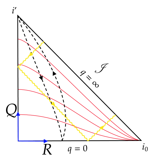
Figure 1: The Penrose diagram of Klein space.

The Penrose diagram can thus be depicted in the $(Q,R)$ coordinates, as shown in Fig. 1. In this diagram, the black dashed line and the yellow wavy line (45°) denote the worldlines of massive and massless particles, respectively. Unlike the Minkowski space $\mathbb{R}^{1,3}$, which has two null boundaries, the Klein space possesses only a single null infinity. This structural difference necessitates replacing the conventional S-matrix with an S-vector to describe scattering processes, following the discussion in Witten:2001kn .

The Klein space admits a natural foliation by $q=$ constant hypersurfaces, represented by red curves in Fig 1, where the $q=0$ limit approaches the hypersurface $Q=0$ and $q\rightarrow\infty$ limit converges to null infinity $\mathscr{I}$. For our subsequent analysis, we employ polar coordinates for the temporal dimensions only while maintaining Cartesian coordinates for the spatial dimensions. This hybrid coordinate system proves particularly advantageous when examining the $q=$ constant hypersurface. Under this choice, the metric takes the form

$$\text{d}s^{2}=-\text{d}q^{2}-q^{2}\text{d}\psi^{2}+(\text{d}x^{2})^{2}+(\text{d}x^{3})^{2}.$$ (7)

The momentum space, as a dual space of Klein space, inherits the same geometric structure as $\mathbb{K}^{2,2}$. Consequently, we can parameterize the 4-momentum using analogous coordinates:

$$p^{\mu}=(p^{0},p^{1},p^{2},p^{3})=(\omega\cos\theta,\omega\sin\theta,\vec{p})\,,\quad\vec{p}=(p^{2},p^{3})\,,\quad\omega>0.$$ (8)

Then the $SO(2,2)$-invariant momentum measure can be defined in the similar manner as that in Minkowski space

$$\int\text{d}^{4}p\delta(p^{2}+m^{2})=\int\omega\text{d}\omega\text{d}\theta\text{d}^{2}\vec{p}\delta(-\omega^{2}+\omega_{\vec{p}}^{2})=\frac{1}{2}\int^{2\pi}_{0}\text{d}\theta\int\text{d}^{2}\vec{p}\bigg{|}_{\omega=\omega_{\vec{p}}}$$ (9)

where

$$\omega=\sqrt{(p^{0})^{2}+(p^{1})^{2}},\qquad\omega_{\vec{p}}=\sqrt{|\vec{p}|^{2}+m^{2}},\qquad|\vec{p}|=\sqrt{(p^{2})^{2}+(p^{3})^{2}}.$$ (10)

The $\vec{p}$ denotes the spacial momentum, and the $\omega_{\vec{p}}$ is the on-shell energy.

3 Canonical quantization for real scalar in Klein space

The canonical quantization of field theories in Minkowski spacetime is fundamentally based on a 3+1 decomposition within the Hamiltonian framework. However, this approach presents a significant challenge when applied to Klein space due to its two equivalent temporal dimensions. The absence of a preferred time direction means that selecting either temporal coordinate would explicitly break the symmetry between them, leading to an ambiguous quantization procedure. To resolve this issue, we introduce a novel quantization scheme that preserves the inherent symmetry of Klein space while maintaining the essential features of canonical quantization. Instead of using one of two temporal coordinates, we adopt the temporal ”radial coordinate” $q$—the invariant length in the time plane-to foliate the space. In this framework, we employ the coordinates specified in (7) to perform the canonical quantization. The induced metric of $q=$ constant hypersurface $\Sigma_{q}$ is then

$$\text{d}s^{2}_{\Sigma_{q}}=-q^{2}\text{d}\psi^{2}+\text{d}\vec{x}^{2},\quad\vec{x}=(x^{2},x^{3}).$$ (11)

Therefore, the determinant of the induced metric is $h=\text{det}[h_{ab}]=-q^{2}$.

In this section, we investigate the canonical quantization for real scalar fields, with the Lagrangian expressed in terms of the coordinates in (7) as

$$\begin{split}\mathcal{L}&=-\frac{1}{2}(\partial_{\mu}\phi\partial^{\mu}\phi+m^{2}\phi^{2})-V(\phi)\\ &=\frac{1}{2}\left[(\partial_{q}\phi)^{2}+\frac{1}{q^{2}}(\partial_{\psi}\phi)^{2}-(\vec{\partial}\phi)^{2}-m^{2}\phi^{2}\right]-V(\phi),\end{split}$$ (12)

where $V(\phi)$ denotes the interacting term relying only on the field $\phi$. The conjugate momentum is then

$$\pi_{q}=\sqrt{h}\frac{\partial\mathcal{L}}{\partial(\partial_{q}\phi)}=iq\partial_{q}\phi.$$ (13)

Therefore, the canonical quantization yields

$$\begin{split}[\phi(q,\psi_{2},\vec{x}_{2}),q\partial_{q}\phi(q,\psi_{1},\vec{x}_{1})]&=\delta(\psi_{12})\delta^{2}(\vec{x}_{12}),\\ [\phi(q,\psi_{1},\vec{x}_{1}),\phi(q,\psi_{2},\vec{x}_{2})]&=0,\end{split}$$ (14)

where

$$\delta(\psi_{12})=\frac{1}{2\pi}\sum_{n\in\mathbb{Z}}e^{in\psi_{12}},\qquad\int^{2\pi}_{0}\text{d}\psi\delta(\psi-\psi^{\prime})f(\psi)=f(\psi^{\prime}).$$ (15)

Before moving on, it is also useful to introduce the definition of Klein-Gordon (KG) inner product between two fields $\phi^{1}$ and $\phi^{2}$

$$\langle\phi^{1},\phi^{2}\rangle\equiv i\int_{\Sigma_{q}}\text{d}\psi\text{d}^{2}x(\phi^{2}\pi^{1}_{q}-\phi^{1}\pi_{q}^{2})=\int_{\Sigma_{q}}\text{d}\psi\text{d}^{2}x\phi^{1}\overset{\longleftrightarrow}{q\partial_{q}}\phi^{2}.$$ (16)

Here we need only partial derivative $\partial_{q}$ rather than covariant derivative, as we are considering scalar fields.

3.1 Free real scalar field

3.1.1 Mode expansion

Let us first consider the free real scalar ($V(\phi)=0$), with the equation of motion (E.o.M)

$$(-\partial^{2}+m^{2})\phi=\left[\frac{1}{q}\partial_{q}(q\partial_{q})+\frac{1}{q^{2}}\partial^{2}_{\psi}+(m^{2}-\vec{\partial}^{2})\right]\phi(q,\psi,\vec{x})=0\,.$$ (17)

The solution can be generally expressed as

$$\phi(q,\psi,\vec{x})=\sum_{n\in\mathbb{Z}}e^{-in\psi}\int\text{d}^{2}\vec{p}e^{i\vec{p}\cdot\vec{x}}f_{n}(q)a_{n,\vec{p}},$$ (18)

where the function $f_{n}(q)$ obeys the equation

$$u^{2}f^{\prime\prime}_{n}(u)+uf^{\prime}_{n}(u)+(u^{2}-n^{2})f_{n}(u)=0,\qquad\omega_{\vec{p}}q=u.$$ (19)

This is the Bessel equation, which has two linearly independent solutions

$$\begin{split}J_{n}(x)&=\sum_{k=0}^{\infty}\frac{(-)^{k}(x/2)^{n+2k}}{k!\Gamma(n+k+1)}=(-)^{n}J_{-n}(x),\\ N_{n}(x)&=\lim_{\nu\rightarrow n}\frac{J_{\nu}(x)\cos\pi\nu-J_{-\nu}(x)}{\sin\pi\nu},\end{split}$$ (20)

where $J_{n},N_{n}$ are referred to as $n$-th order Bessel function and Neumann function (also called Bessel function of the second kind), and they form the Bessel basis as the solutions of the Klein Gordon equation when multiplied with $e^{-in\psi+i\vec{p}\cdot\vec{x}}$. However, based on the following asymptotic behavior of $N_{n},J_{n}$

$$\begin{split}&x\rightarrow 0:\ \begin{cases}&J_{0}(x)\rightarrow 1,\quad J_{n\neq 0}\rightarrow\frac{1}{n!}\left(\frac{x}{2}\right)^{n},\\ &N_{0}(x)\sim\frac{2}{\pi}\ln x,\quad N_{n\neq 0}(x)\rightarrow-\frac{(n-1)!}{\pi}\left(\frac{2}{x}\right)^{n}\end{cases}\\ &x\rightarrow\infty:\ \begin{cases}&J_{n}(x)\rightarrow\sqrt{\frac{2}{\pi x}}\cos\left(x-\frac{n}{2}\pi-\frac{\pi}{4}\right)\\ &N_{n}(x)\rightarrow\sqrt{\frac{2}{\pi x}}\sin\left(x-\frac{n}{2}\pi-\frac{\pi}{4}\right)\end{cases},\end{split}$$ (21)

the Neumann function $N_{n}(\omega_{\vec{p}}q)$ is divergent when $q\rightarrow 0$. Therefore, the $N_{n}$ modes are forbidden in the classical solution, as the field $\phi(x)$ must remain finite for any value of the coordinates at the classical level. As a result, the classical solution is given by

$$\phi^{\text{cl}}(q,\psi,\vec{x})=\sqrt{\frac{\pi}{2}}\sum_{n\in\mathbb{Z}}\int\frac{\text{d}^{2}\vec{p}}{(2\pi)^{3}}a^{(J)}_{n,\vec{p}}J_{n}(\omega_{\vec{p}}q)e^{i(\vec{p}\cdot\vec{x}-n\psi)},$$ (22)

where the superscript “cl” is the abbreviation of “classical”, and $a^{(J)}$ is independent of the coordinates $(q,\psi,\vec{x})$. The reality condition $\phi^{*}=\phi$ is then equivalent to

$$a_{n,\vec{p}}^{(J)*}=(-)^{n}a_{-n,-\vec{p}}^{(J)}\,,$$ (23)

because of $J_{n}=(-)^{n}J_{-n}$.

The mode expansion (22) indicates that there are no two linearly independent modes for the classical solution in Klein space. This becomes much clearer when compared to the Minkowski case. To facilitate this comparison, we re-express the classical solution (22) in terms of plane-wave modes using Cartesian coordinates as

$$\phi^{\text{cl}}(q,\psi,\vec{x}) =\frac{1}{2}\int\frac{\text{d}^{4}p}{(2\pi)^{3}}\delta(p^{2}+m^{2})a_{p}^{(J)}e^{ipx}$$ (24)

$$=\frac{1}{4}\int\frac{\text{d}\theta\text{d}^{2}\vec{p}}{(2\pi)^{3}}a_{\theta,\vec{p}}^{(J)}e^{i(-\omega_{\vec{p}}q\cos(\theta-\psi)+\vec{p}\cdot\vec{x})}\,,$$

where $\theta$ is the polar angle of the momentum component $p^{0},p^{1}$, and we used the integral representation of Bessel function

$$J_{n}(\omega_{\vec{p}}q)=\frac{i^{n}}{2\pi}\int_{-\pi}^{\pi}\text{d}\theta e^{-in\theta}e^{-i\omega_{\vec{p}}q\cos\theta}\,,$$ (25)

and the relation between the coefficients

$$a_{\theta,\vec{p}}^{(J)}=a_{p}^{(J)}\Big{|}_{p^{2}+m^{2}=0}=\sqrt{\frac{2}{\pi}}\sum_{n\in\mathbb{Z}}i^{n}a_{n,\vec{p}}^{(J)}e^{in\theta}\,,$$ (26)

In comparison, the mode expansions via plane waves in Minkowski

$$\phi^{\text{cl}}_{\text{Mink}}(t,\vec{x})=\int\frac{\text{d}^{3}\vec{p}}{(2\pi)^{3}2\omega_{\vec{p}}}\left[a_{\vec{p}}e^{-i\omega_{\vec{p}}t+i\vec{p}\cdot\vec{x}}+a^{*}_{-\vec{p}}e^{i\omega_{\vec{p}}t+i\vec{p}\cdot\vec{x}}\right]\,,$$ (27)

do have two linearly independent modes $e^{-i\omega_{\vec{p}}t+i\vec{p}\cdot\vec{x}}$ and $e^{i\omega_{\vec{p}}t+i\vec{p}\cdot\vec{x}}$. In Minkowski spacetime, the creation and annihilation operators can create plane wave modes at the past infinity and the future infinity, respectively. Thus, there must be two independent modes associated with two different conformal boundaries. But in Klein space, whose Penrose diagram is topologically equivalent to gluing together the two conformal boundaries of the Penrose diagram of Minkowski spacetime, there is only one conformal boundary. The gluing of the boundaries transforms the worldlines of massive plane waves to closed curves (see the black dashed line in Fig. 1) , which means that the outgoing and incoming processes of plane waves on the single conformal boundary are no longer two independent processes. Instead, they are identical to each other.

However, only one linearly independent mode causes some severe problems. One is that the classical free fields $\phi$ are not independent of their conjugation $\pi_{q}=iq\partial_{q}\phi$. This can be shown by using the KG inner product. Note that the dual of the Klein-Gordon current $J^{12}:=\phi^{1}\overleftrightarrow{\partial_{\mu}}\phi^{2}\text{d}x^{\mu}$ constructed by the on-shell fields $\phi^{1},\phi^{2}$ is closed

$$\text{d}*J^{12}=-\partial^{\mu}\left(\phi^{1}\overleftrightarrow{\partial_{\mu}}\phi^{2}\right)\text{d}^{4}x=m^{2}\phi^{1}\phi^{2}-m^{2}\phi^{1}\phi^{2}=0,$$ (28)

which has also been demonstrated in Melton:2024pre for massless case. This results in the vanishing of the KG inner product between two fields

$$\langle\phi^{1},\phi^{2}\rangle\propto\int_{\Sigma_{q_{0}}}*J^{12}=\int_{M_{4}}\text{d}*J^{12}=0.$$ (29)

Here, the hypersurfaces $\Sigma_{q_{0}}$ are always the boundary $\partial M_{4}$ of a four-dimensional region $M_{4}\equiv\{(q,\psi,\vec{x})|0\leq q\leq q_{0}\}$. In particular, provided that the field $\phi$ is on-shell, the conjugate momentum $\pi_{q}=iq\partial_{q}\phi$ also satisfies the Klein-Gordon equation, indicating the vanishing of the inner product

$$\langle\phi^{\text{cl}},\pi_{q}\rangle=0,$$ (30)

The vanishing of the inner product indicates the linear dependence of $\phi$ and $\pi_{q}$. As a result, it is not possible to satisfy the two relations in (14) simultaneously when dealing with the canonical quantization.

The other more technical problem is that when we consider amplitudes in flat space, we need to use the KG inner product

$$\langle e^{\pm ipx},\phi^{\text{cl}}(x)\rangle=0\,,$$ (31)

to define an asymptotic scattering state, see (77) and (78) later. But here it just vanishes due to the same reason as in the above discussions.

To overcome these problems, it is essential to introduce additional modes besides the ones relating to Bessel function. These additional modes could emerge at the quantum level, while they are forbidden at the classical level. The Neumann modes $N_{n}$, previously discarded by the classical regular condition at $q=0$, are appropriate candidates. They can be retrieved by removing the original point in the Klein space to obtain a new manifold $\mathbb{K}^{2,2}-\{0\}$, where the quantum fields are defined. Then, the Klein-Gordon inner product between on-shell fields will no longer vanish, because the $\Sigma_{q_{0}}$ in (29) is not the only boundary of $M_{4}-\{0\}\equiv\{(q,\psi,\vec{x})|0<q\leq q_{0}\}$. Consequently, $\phi$ and $\pi_{q}$ are independent after introducing $N_{n}$. Furthermore, the classical requirement for the field $\phi$ to be regular at $q=0$ is modified in the quantum level: we only require its regularity when acting on the vacuum state $\ket{0}$

$$\phi(q,\psi,\vec{x})\ket{0}\Big{|}_{q=0}=\text{finite}.$$ (32)

This is analogous to the definition of asymptotic states in CFT DiFrancesco:1997nk . As a result, the mode expansion of free scalar field should be reformulated as

$$\phi(q,\psi,\vec{x})=\sqrt{\frac{\pi}{2}}\sum_{n\in\mathbb{Z}}\int\frac{\text{d}^{2}\vec{p}}{(2\pi)^{3}}\left[a^{(J)}_{n,\vec{p}}J_{n}(\omega_{\vec{p}}q)+a^{(N)}_{n,\vec{p}}N_{n}(\omega_{\vec{p}}q)\right]e^{i(\vec{p}\cdot\vec{x}-n\psi)}\,.$$ (33)

Here, $a^{(J)}$ and $a^{(N)}$ are linearly independent operators.The reality condition is then given by

$$a^{(J)*}_{n,\vec{p}}=(-)^{n}a^{(J)}_{-n,-\vec{p}}\,,\quad a^{(N)*}_{n,\vec{p}}=(-)^{n}a^{(N)}_{-n,-\vec{p}}\,,$$ (34)

because of $N_{n}=(-)^{n}N_{-n},\ J_{n}=(-)^{n}J_{-n}$. The regular condition (32) is explicitly given by

$$a^{(N)}_{n,\vec{p}}\ket{0}=0\quad(\forall n,\vec{p}),$$ (35)

as the $q=0$ divergences come from $N_{n}$ modes. Since the state $|0\rangle$ is annihilated by the Neunmann function coefficient, we will call it the Neumann vacuum, in contrast with the Hankel vacuum $\langle\infty|$ which will be defined in (59) later. Now the Klein-Gordon product between the plane-wave and the field is not vanishing

$$\begin{split}\langle e^{-ip\cdot x},\phi(x)\rangle&=\sqrt{\frac{\pi}{2}}\sum_{n\in\mathbb{Z}}i^{n}e^{in\theta}a^{(N)}_{n,\vec{p}}J_{n}(\omega_{\vec{p}}q)\overset{\longleftrightarrow}{q\partial_{q}}N_{n}(\omega_{\vec{p}}q)\end{split}$$ (36)

The above equation is independent of $q$, due to the following identity

$$J_{n}(\omega_{\vec{p}}q)\overset{\longleftrightarrow}{q\partial_{q}}N_{n}(\omega_{\vec{p}}q)=\frac{2}{\pi}\qquad(\forall q\geq 0).$$ (37)

Then, one obtains

$$a^{(N)}_{\theta,\vec{p}}\equiv\sqrt{\frac{2}{\pi}}\sum_{n\in\mathbb{Z}}i^{n}e^{in\theta}a^{(N)}_{n,\vec{p}}=\langle e^{-ip\cdot x},\phi(x)\rangle.$$ (38)

For convenience, one can perform Fourier transformation to Eq.(38) and obtains

$$\begin{split}a_{n,\vec{p}}^{(N)}&=\sqrt{\frac{\pi}{2}}\left\langle e^{-i(\vec{p}\cdot\vec{x}-n\psi)}J_{n}(\omega_{\vec{p}}q),\phi(q,\psi,\vec{x})\right\rangle\\ &=-\sqrt{\frac{\pi}{2}}\int\frac{\text{d}^{2}\vec{x}\text{d}\psi}{(2\pi)^{3}}e^{-i(\vec{p}\cdot\vec{x}-n\psi)}\phi(q,\psi,\vec{x})\overset{\longleftrightarrow}{q\partial_{q}}J_{n}(\omega_{\vec{p}}q).\end{split}$$ (39)

Similarly, the $a_{n,\vec{p}}^{(J)}$ can also be derived in terms of the Klein-Gordon inner product as

$$\begin{split}a_{n,\vec{p}}^{(J)}&=-\sqrt{\frac{\pi}{2}}\left\langle e^{-i(\vec{p}\cdot\vec{x}-n\psi)}N_{n}(\omega_{\vec{p}}q),\phi(q,\psi,\vec{x})\right\rangle\\ &=\sqrt{\frac{\pi}{2}}\int\frac{\text{d}^{2}\vec{x}\text{d}\psi}{(2\pi)^{3}}e^{-i(\vec{p}\cdot\vec{x}-n\psi)}\phi(q,\psi,\vec{x})\overset{\longleftrightarrow}{q\partial_{q}}N_{n}(\omega_{\vec{p}}q).\end{split}$$ (40)

It is important to reiterate that the Eqs (40) and (39) hold for any $q$, because their left-hand sides are all independent of $q$. The canonical quantization (14) is thus equivalent to

$$\left[a^{(J)}_{n,\vec{p}_{1}},a^{(N)}_{m,\vec{p}_{2}}\right]=(-)^{n}(2\pi)^{3}\delta_{m+n,0}\delta^{2}(\vec{p}_{1}+\vec{p}_{2})$$ (41)

or equivalently,

$$\left[a^{(J)}_{n,\vec{p}_{1}},a^{(N)*}_{m,\vec{p}_{2}}\right]=(2\pi)^{3}\delta_{m,n}\delta^{2}(\vec{p}_{12}).$$ (42)

3.1.2 Hamiltonian and evolution operator

The Hamiltonian of the free real scalar can be derived from the Legendre transformation of the Lagrangian

$$\begin{split}H_{q}^{(0)}&=\int q\text{d}\psi\text{d}^{2}\vec{x}(\phi\partial_{q}\phi-\mathcal{L})\\ &=\frac{1}{2}\int\text{d}\psi\text{d}^{2}\vec{x}\left[-\frac{1}{q}\pi_{q}^{2}-\frac{1}{q}(\partial_{\psi}\phi)^{2}+(\vec{\partial}\phi)^{2}+m^{2}\phi^{2}\right].\end{split}$$ (43)

The Hamiltonian is then $q$-dependent. Furthermore, the Hamiltonians at different values of $q$ do not commute with each other, while Hamiltonians at the same $q$ commute

$$\left[H^{(0)}_{q_{1}},H^{(0)}_{q_{2}}\right]\neq 0,\quad\left[H^{(0)}_{q},H^{(0)}_{q}\right]=0.$$ (44)

The commutators between $H^{(0)}_{q}$ and the field $\phi$ or the conjugation momentum $\pi_{q}$ at the same $q$ are derived from the canonical commutator (14) as

$$\begin{split}\left[H^{(0)}_{q},\phi(q,\psi,\vec{x})\right]&=-\partial_{q}\phi(q,\psi,\vec{x}),\\ \left[H^{(0)}_{q},\pi_{q}(q,\psi,\vec{x})\right]&=-\partial_{q}\pi_{q}(q,\psi,\vec{x}),\end{split}$$ (45)

which are the Heisenberg equations. The solution of the Heisenberg equations are

$$\begin{split}\phi(q,\psi,\vec{x})&=U^{-1}_{(0)}(q,q_{0})\phi(q_{0},\psi,\vec{x})U_{(0)}(q,q_{0})\,,\\ \pi_{q}(q,\psi,\vec{x})&=U^{-1}_{(0)}(q,q_{0})\pi_{q_{0}}(q_{0},\psi,\vec{x})U_{(0)}(q,q_{0})\,.\end{split}$$ (46)

Here, $q_{0}$ is the reference time (or initial time), and the evolution operator $U_{(0)}(q,q_{0})$ with the initial condition $U_{(0)}(q_{0},q_{0})=1$ satisfies the schr$\ddot{\text{o}}$dinger equation

$$\partial_{q}U_{(0)}(q,q_{0})=U_{(0)}(q,q_{0})H_{q}^{(0)},\quad\partial_{q}U^{-1}_{(0)}(q,q_{0})=-H_{q}^{(0)}U^{-1}_{(0)}(q,q_{0}).$$ (47)

These two equations are actually equivalent, and they have the solution

$$U_{(0)}(q,q_{0})=\mathcal{Q}^{-1}\text{exp}\left[\int^{q}_{q_{0}}H^{(0)}_{q^{\prime}}\text{d}q^{\prime}\right]\quad\text{when}\ q>q_{0}\,,$$ (48)

and

$$U_{(0)}(q,q^{\prime})=U^{-1}_{(0)}(q^{\prime},q)\quad\text{when}\ q<q^{\prime}\,,$$ (49)

where $\mathcal{Q}^{-1}$ is the anti-$q$ order operator placing the operators with larger $q$ on the right. Note that $H_{q}^{(0)}$ is actually the Hamiltonian in the Heisenberg picture. The evolution operator $U_{(0)}(q,q_{0})$ takes a complex form because the fact that $H_{q}^{(0)}$’s at different $q$ do not commute with each other.

The Hamiltonian in the Schr$\ddot{\text{o}}$dinger picture is

$$\begin{split}H_{q}^{(0)(S)}&=U_{(0)}(q,q_{0})H_{q}^{(0)}U^{-1}_{(0)}(q,q_{0})\\ &=\frac{1}{2}\int\text{d}\psi\text{d}^{2}\vec{x}\left[-\frac{1}{q}\pi_{q_{0}}^{2}-\frac{1}{q}(\partial_{\psi}\phi(q_{0}))^{2}+(\vec{\partial}\phi(q_{0}))^{2}+m^{2}(\phi(q_{0}))^{2}\right],\end{split}$$ (50)

where $\phi(q_{0})$ is a shorthand version of $\phi(q_{0},\psi,\vec{x})$. The Hamitonian in these two pictures are linked at the initial time $q_{0}$

$$H^{(0)(S)}_{q_{0}}=H^{(0)}_{q_{0}}.$$ (51)

Note that even in the Schr$\ddot{\text{o}}$dinger picture, the Hamiltonian for free scalar still depends on $q$, and

$$\left[H^{(0)(S)}_{q_{1}},H^{(0)(S)}_{q_{2}}\right]\neq 0\quad(q_{1}\neq q_{2}),\quad\quad\left[H^{(0)(S)}_{q},H^{(0)(S)}_{q}\right]=0.$$ (52)

The Heisenberg equation (47) can be rewritten in term of $H^{(0)(S)}_{q}$ as

$$\partial_{q}U_{(0)}(q,q_{0})=H^{(0)(S)}_{q}U_{(0)}(q,q_{0}).$$ (53)

Then, the evolution operator can be expressed in terms of Hamiltonian in the Schr$\ddot{\text{o}}$dinger picture as

$$U_{(0)}(q,q_{0})=\mathcal{Q}\text{exp}\left[\int^{q}_{q_{0}}H^{(0)(S)}_{q^{\prime}}\text{d}q^{\prime}\right],\quad\text{when}\ q>q_{0}$$ (54)

where $\mathcal{Q}$ represents the $q$-ordering operator placing the fields with larger $q$ to the left of those with smaller $q$.

3.1.3 Correlation functions

On the other hand, the quantum field theory in Klein space can also be regarded as the analytical continuation from Euclidean space by implementing Wick rotation $q_{E}\rightarrow iq(1-i\epsilon)$. Here, $q_{E}$ denotes the radial direction on 2D plane $(x^{0}_{E},x^{1}_{E})$ in Euclidean space parametrized by the coordinates $(x^{0}_{E},x^{1}_{E},x^{2},x^{3})$. This is similar to the analytical continuation from Euclidean space to Minkowski space $x^{0}_{E}\rightarrow ix^{0}(1-i\epsilon)$, which leads to the $x^{0}$-ordered (time-ordered) correlation function. For more information about Wick rotation, see Appendix A. Therefore, the $n$-point correlation function for QFT in Klein space is similarly defined by the $q$-ordered expectation of $n$ operators, expressed as

$$\langle\phi_{1}(x_{1})\cdots\phi_{n}(x_{n})\rangle=\bra{\infty}\mathcal{Q}\phi_{1}(x_{1})\cdots\phi_{n}(x_{n})\ket{0}\,.$$ (55)

Instead of using $\bra{0}$, we adopt the state $\bra{\infty}$ as the bra vacuum state in the correlation function, because here we need to work in an “in-out” formalism rather than an “in-in” formalism. The “in-out” formalism can be translated to the usual path integral and related to the results from analytical continuation, while the “in-in” formalism can be translated to a closed-time-path functional integral Schwinger:1960qe . The field $\phi$ at the asymptotic infinity behaves as

$$\phi(q,\psi,\vec{x}) =\sqrt{\frac{\pi}{2}}\sum_{n\in\mathbb{Z}}\int\frac{\text{d}^{2}\vec{p}}{(2\pi)^{3}}\left[a^{(H^{(1)})}_{n,\vec{p}}H_{n}^{(1)}(\omega_{\vec{p}}q)+a^{(H^{(2)})}_{n,\vec{p}}H_{n}^{(2)}(\omega_{\vec{p}}q)\right]e^{i(\vec{p}\cdot\vec{x}-n\psi)}$$ (56)

$$\underset{q\to\infty}{\longrightarrow}\sqrt{\frac{\pi}{2}}\sum_{n\in\mathbb{Z}}\int\frac{\text{d}^{2}\vec{p}}{(2\pi)^{3}}\sqrt{\frac{2}{\pi\omega_{\vec{p}}q}}\left[a^{(H^{(1)})}_{n,\vec{p}}e^{i\left(\omega_{\vec{p}}q-\frac{n\pi}{2}-\frac{\pi}{4}\right)}+a^{(H^{(2)})}_{n,\vec{p}}e^{-i\left(\omega_{\vec{p}}q-\frac{n\pi}{2}-\frac{\pi}{4}\right)}\right]e^{i(\vec{p}\cdot\vec{x}-n\psi)}$$

with

$$a^{(H^{(1)})}_{n,\vec{p}}=\frac{a^{(J)}_{n,\vec{p}}-ia^{(N)}_{n,\vec{p}}}{2}\,,\quad a^{(H^{(2)})}_{n,\vec{p}}=\frac{a^{(J)}_{n,\vec{p}}+ia^{(N)}_{n,\vec{p}}}{2}\,,$$ (57)

where we reformulated the mode expansion (33) by the first-kind and the second kind Hankel functions $H^{(1)}_{n}(x)$ and $H^{(2)}_{n}(x)$ defined as

$$H_{n}^{(1)}(x)=J_{n}(x)+iN_{n}(x)\,,\quad H_{n}^{(2)}(x)=J_{n}(x)-iN_{n}(x)\,.$$ (58)

The modes $e^{i\left(\omega_{\vec{p}}q-\frac{n\pi}{2}-\frac{\pi}{4}\right)}$ and $e^{-i\left(\omega_{\vec{p}}q-\frac{n\pi}{2}-\frac{\pi}{4}\right)}$ are similar to $e^{i\omega t}$ and $e^{-i\omega t}$ in the Minkowski case. Thus, one of them should be interpreted as the annihilation operator and the other as the creation operator concerning the state $\langle\infty|$. We will see that the right choice is

$$\langle\infty|a_{n,\vec{p}}^{(H^{(1)})}=0\,.$$ (59)

Since the state $\langle\infty|$ is annihilated by the Hankel function coefficient acting from the right side, we will call it the Hankel vacuum. Now we can calculate any correlation functions via the Wick contraction, based on the annihilation conditions of Neumann vacuum (35) and the Hankel vacuum (59). Let us consider the two-point propagator $\Delta(x-x^{\prime})=\langle\infty|\mathcal{Q}\phi(x)\phi(x^{\prime})|0\rangle$ as an example. By using the Poincaré symmetry, we can always transform the two points to locate at $x=(q,\psi,\vec{x}),\,x^{\prime}=(0,0,\vec{0})$, then we have

$$\langle\infty|\phi(x)\phi(0)|0\rangle =\frac{\pi}{2}\sum_{n}\int\frac{\text{d}^{2}\vec{p}\text{d}^{2}\vec{p}^{\prime}}{(2\pi)^{6}}e^{i(\vec{p}\cdot\vec{x}-n\psi)}H_{n}^{(2)}(\omega_{\vec{p}}q)\langle\infty|a_{n,\vec{p}}^{(H^{(2)})}a_{0,\vec{p}^{\prime}}^{(J)}|0\rangle$$ (60)

$$=-\frac{i\pi}{2}\int\frac{\text{d}^{2}\vec{p}}{(2\pi)^{3}}H_{0}^{(2)}(\omega_{\vec{p}}q)e^{i\vec{p}\cdot\vec{x}}\,\langle\infty|0\rangle.$$

where we used the commutator (41) in the last step. Note that the inner product $\langle\infty|0\rangle$ is non-vanishing.

In general, the two-point propagator can be expressed in a covariant form. This can be achieved by acting Klein-Gordon operator $-\partial^{2}+m^{2}$ on the two-point function

$$\begin{split}&\left(\frac{\partial_{q}}{q}(q\partial_{q})+\frac{\partial_{\phi}^{2}}{q^{2}}-\vec{\partial}^{2}+m^{2}\right)\langle\infty|\mathcal{Q}\phi(x)\phi(x^{\prime})|0\rangle\\ &=\frac{\partial_{q}}{q}\eta(q-q^{\prime})\bra{\infty}[q\partial_{q}\phi(x),\phi(x^{\prime})]\ket{0}\,,\end{split}$$ (61)

where $\eta(x)$ denotes the step function. This differential equation can be re-expressed by using (14)

$$\begin{split}(-\partial_{x}^{2}+m^{2})\Delta(x-x^{\prime})&=-\frac{1}{q}\delta(q-q^{\prime})\delta(\psi-\psi^{\prime})\delta^{2}(\vec{x}-\vec{x}^{\prime})\bra{\infty}0\rangle\\ &=-\delta^{4}(x-x^{\prime})\bra{\infty}0\rangle\,.\end{split}$$ (62)

The solution of this equation is

$$\Delta(x-x^{\prime})=-\int\frac{\text{d}^{4}p}{(2\pi)^{4}}\frac{e^{ip(x-x^{\prime})}}{p^{2}+m^{2}-i\epsilon}\bra{\infty}0\rangle\,.$$ (63)

The above expression matches the result (60) derived from the Wick contraction, see details in the Appendix B. This also serves as the verification of the annihilation condition (59) for the Hankel vacuum $\bra{\infty}$.

3.2 The interacting real scalar field and LSZ reduction formula

For the interacting real scalar, the potential $V(\phi)$ in the Lagrangian is non-vanishing, such that the E.o.M (17) should be modified to include potential terms. In a QFT textbook, people usually use the interaction picture, which is convenient for perturbative calculations, see appendix C. However, in this subsection, we adopt the Heisenberg picture in which the mode expansion can be formally performed in a similar form to that of free field theory (33),

$$\phi(q,\psi,\vec{x})=\sqrt{\frac{\pi}{2}}\sum_{n\in\mathbb{Z}}\int\frac{\text{d}^{2}\vec{p}}{(2\pi)^{3}}\left[a^{(J)}_{n,\vec{p}}(q)J_{n}(\omega_{\vec{p}}q)+a^{(N)}_{n,\vec{p}}(q)N_{n}(\omega_{\vec{p}}q)\right]e^{i(\vec{p}\cdot\vec{x}-n\psi)}\,.$$ (64)

But now the coefficients $a^{(J)}(q),a^{(N)}(q)$ are no longer independent of the coordinate $q$. As a result, they do not satisfy (41) except for $q\rightarrow\infty$ where the field tends to be free. As usual, the reality condition also yields

$$a^{(J)*}_{n,\vec{p}}(q)=(-)^{n}a^{(J)}_{-n,-\vec{p}}(q)\,,\quad a^{(N)*}_{n,\vec{p}}(q)=(-)^{n}a^{(N)}_{-n,-\vec{p}}(q)\,.$$ (65)

The interacting field $\phi$ also satisfies the Heisenberg equation

$$\partial_{q}\phi=-[H_{q},\phi]\,,$$ (66)

where the Hamiltonian for interacting real scalar theory is given by

$$\begin{split}H_{q}&=H_{q}^{(0)}+H_{q}^{(\text{int})}\\ &=\frac{1}{2}\int\text{d}\psi\text{d}^{2}\vec{x}\left[-\frac{1}{q}\pi_{q}^{2}-\frac{1}{q}(\partial_{\psi}\phi)^{2}+(\vec{\partial}\phi)^{2}+m^{2}\phi^{2}\right]+\int q\text{d}\psi\text{d}^{2}\vec{x}V(\phi)\,.\end{split}$$ (67)

Therefore, the interacting field $\phi$ evolves as

$$\phi(q,\psi,\vec{x})=U^{-1}(q,q_{0})\phi(q_{0},\psi,\vec{x})U(q,q_{0})$$ (68)

where the evolution operator $U(q,q_{0})$ satisfies the Schr$\ddot{\text{o}}$dinger equation

$$\partial_{q}U(q,q_{0})=U(q,q_{0})H_{q},$$ (69)

the solution of which is

$$U(q,q_{0})=\mathcal{Q}^{-1}\text{exp}\left[\int^{q}_{q_{0}}H_{q^{\prime}}\text{d}q^{\prime}\right].$$ (70)

The evolution operator can also be expressed by using the Hamiltonian in the Schr$\ddot{\text{o}}$dinger picture. This is similar to the discussion in section 3.1.2, and we will not repeat it here.

Moreover, at the quantum level, $\phi(q\rightarrow 0)|0\rangle$ also needs to be finite, leading to

$$a^{(N)}_{n,\vec{p}}(q=0)\ket{0}=0\qquad\forall n,\vec{p}\,,$$ (71)

or equivalently,

$$a^{(N)}_{\theta,\vec{p}}(q=0)\ket{0}=0\qquad\forall\theta,\vec{p}\,.$$ (72)

In general, $a^{(N)}_{\theta,\vec{p}}(q=\infty)\ket{0}\neq 0$ as $a^{(N)}_{\theta,\vec{p}}(\infty)$ differs from $a_{\theta,\vec{p}}^{(N)}(0)$ in a non-trivial way. This can be shown by computing the following Klein-Gordon inner product

$$\langle e^{-ip\cdot x},\phi(x)\rangle\Big{|}_{q}=\sqrt{\frac{\pi}{2}}\sum_{n\in\mathbb{Z}}i^{n}e^{in\theta}J_{n}(\omega_{\vec{p}}q)\overset{\longleftrightarrow}{q\partial_{q}}\left[a^{(J)}_{n,\vec{p}}(q)J_{n}(\omega_{\vec{p}}q)+a^{(N)}_{n,\vec{p}}(q)N_{n}(\omega_{\vec{p}}q)\right].$$ (73)

Fortunately, through the asymptotic behavior of the Bessel functions (21), one can find that

$$a^{(N)}_{\theta,\vec{p}}(q)\equiv\sqrt{\frac{2}{\pi}}\sum_{n\in\mathbb{Z}}i^{n}e^{in\theta}a^{(N)}_{n,\vec{p}}(q)=\langle e^{-ipx},\phi(x)\rangle\Big{|}_{q}\,,\quad\text{when}\ q\rightarrow 0,\infty.$$ (74)

Now with the Klein-Gordon product at the asymptotic region $(q\rightarrow 0,\infty)$, we can calculate the difference between $a^{(N)}_{\theta,\vec{p}}(\infty)$ and $a_{\theta,\vec{p}}^{(N)}(0)$ as

$$\begin{split}a^{(N)}_{\theta,\vec{p}}(\infty)-a^{(N)}_{\theta,\vec{p}}(0)=&\langle e^{-ipx},\phi(x)\rangle\Big{|}_{q=0}^{\infty}=\int\text{d}\psi\text{d}^{2}\vec{x}\left[e^{-ipx}\overset{\longleftrightarrow}{q\partial_{q}}\phi(x)\right]\Big{|}_{q=0}^{\infty}\\ =&\int\text{d}^{4}xe^{-ipx}(-\partial^{2}+m^{2})\phi(x)\,.\end{split}$$ (75)

The difference will be important in deriving the LSZ reduction formula.

The scattering amplitude is defined by the inner product between the scattering state living on the boundary of Klein space and the S-vector $|S\rangle\equiv|0\rangle$ (originally mentioned in section 2), or more explicitly

$$\mathcal{A}_{n}:=\langle p_{1},\cdots,p_{n}|S\rangle=\langle\infty|a_{p_{1}}(\infty)\cdots a_{p_{n}}(\infty)|0\rangle,$$ (76)

where the scattering state defined at the asymptotic region $q\rightarrow\infty$ is given by

$$\langle p_{1},\cdots,p_{n}| =\langle\infty|a_{p_{1}}(\infty)\cdots a_{p_{n}}(\infty).$$ (77)

The explicit expression for the counterpart of $a_{p}$ in Minkowski space is the Klein-Gordon inner product between the plane wave and the field $\phi(x)$. In Klein space, $a_{p}$ can be similarly defined as the plane wave generator $\langle e^{-ipx},\phi(x)\rangle$ in the asymptotic regions $q\rightarrow 0,\infty$,

$$a_{p}(q):=\langle e^{-ipx},\phi(x)\rangle=a^{(N)}_{\theta,\vec{p}}(q),\quad\text{when}~~q\rightarrow 0,\infty,$$ (78)

where the expression for $a^{(N)}_{\theta,\vec{p}}(q=0,\infty)$ has been shown in (74). Therefore, the amplitude can be rewritten in terms of the Klein-Gordon inner products $\langle e^{-ipx},\phi(x)\rangle$

$$\mathcal{A}_{n} =\langle\infty|\mathcal{Q}\left(a^{(N)}_{\theta_{1},\vec{p}_{1}}(\infty)-a^{(N)}_{\theta_{1},\vec{p}_{1}}(0)\right)\cdots\left(a^{(N)}_{\theta_{n},\vec{p}_{n}}(\infty)-a^{(N)}_{\theta_{n},\vec{p}_{n}}(0)\right)|0\rangle$$ (79)

$$=\langle\infty|\mathcal{Q}\langle e^{-ip_{1}x_{1}},\phi(x_{1})\rangle\Big{|}_{q=0}^{\infty}\cdots\langle e^{-ip_{n}x_{n}},\phi(x_{n})\rangle\Big{|}_{q=0}^{\infty}|0\rangle$$

where we use the regularity condition (72) to add the $a^{(N)}_{\theta_{i},\vec{p}_{i}}(0)\ket{0}$ term. Note that the $a^{(N)}_{\theta_{i},\vec{p}_{i}}(\infty)$ generally do not commute with $a^{(N)}_{\theta_{i},\vec{p}_{i}}(0)$, because $a^{(N)}_{\theta_{i},\vec{p}_{i}}(\infty)$ are expressed in terms of $a^{(N)}_{\theta_{i},\vec{p}_{i}}(0),a^{(J)}_{\theta_{i},\vec{p}_{i}}(0)$. Therefore, the $q$-ordering operator $\mathcal{Q}$ is necessary to move all $a^{(N)}_{\theta_{i},\vec{p}_{i}}(0)$ attached to $\ket{0}$. Finally, by using the equation (75), we have

$$\mathcal{A}_{n}=\left[\prod^{n}_{k=1}\int\text{d}^{4}x_{k}e^{-ip_{k}x_{k}}(-\partial_{k}^{2}+m^{2})\right]\langle\infty|\mathcal{Q}\phi(x_{1})\cdots\phi(x_{n})|0\rangle\,.$$ (80)

This is in the same form as the LSZ reduction formula in Minkowski space. In particular, in the case of free theory, in which $a^{(N)}_{n,\vec{p}}(q=0)=a^{(N)}_{n,\vec{p}}(q=\infty)$, the amplitude will vanish.

4 Path-integral formalism

In this section, we will study a generally interacting real scalar field in the path-integral formalism. We will start from the path-integral formalism in Euclidean space $(x^{0}_{E},x^{1}_{E},x^{2},x^{3})$ to define the ket vacuum state $|0\rangle$, the bra vacuum $\langle\infty|$, and the $q$-evolution operator $U(q,q^{\prime})$, and then turn to Klein space by implementing the Wick rotation $q_{E}=\sqrt{(x^{0}_{E})^{2}+(x^{1}_{E})^{2}}\rightarrow iq(1-i\epsilon)$. Finally, we will derive the LZS reduction formula that bridges the correlation functions and scattering amplitudes. The canonical quantization results will also be reproduced in terms of the path integral.

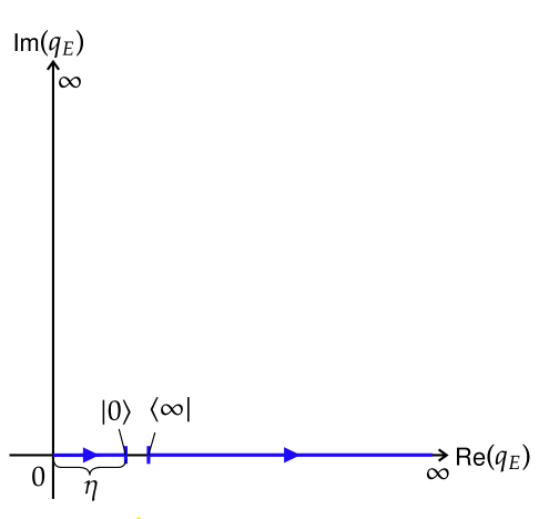
(a) The definitions of $\bra{\infty}$ and $\ket{0}$.

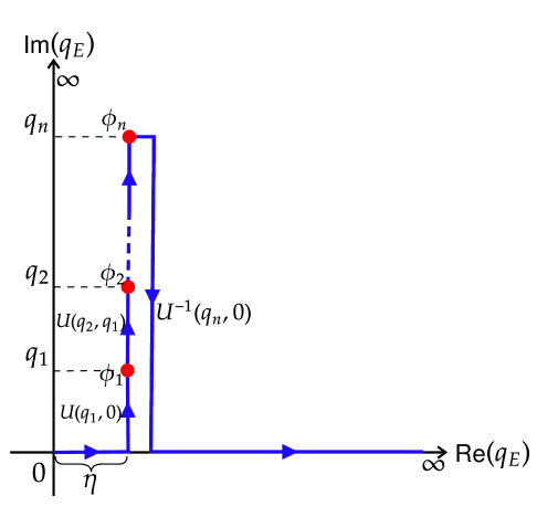
(b) The $q$-ordered $n$-point correlation function $\bra{\infty}\phi_{n}(x_{n})\cdots\phi_{1}(x_{1})\ket{0}$, where $q_{1}<\cdots<q_{n}$.

Figure 2: The path integral approach to define vacuum states and correlation functions in the Euclidean signature. The complex plane here is described by the complexified $q_{E}$.

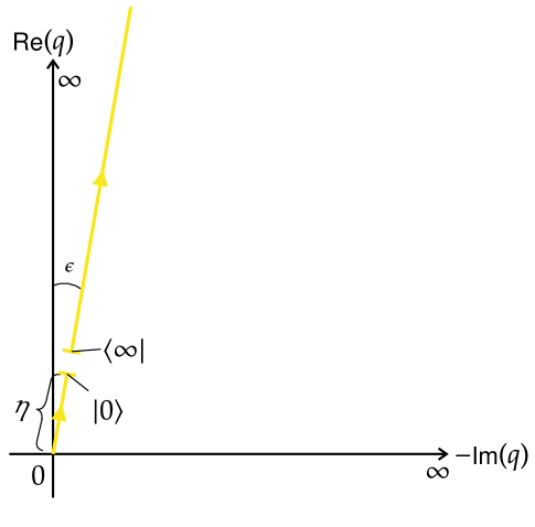
(a) The definitions of $\bra{\infty}$ and $\ket{0}$.

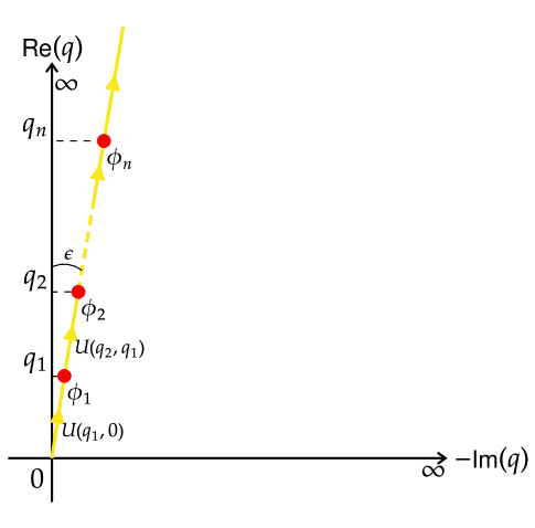
(b) The $q$-ordered $n$-point correlation function $\bra{\infty}\phi_{n}(x_{n})\cdots\phi_{1}(x_{1})\ket{0}$, where $q_{1}<\cdots<q_{n}$.

Figure 3: The path integral approach to define vacuum states and correlation functions in the Klein signature. The complex plane here is described by the complexified $q$ with $q=-iq_{E}$

A general state $|\Psi\rangle$ in a quantum field theory is a wave functional which maps a field $\tilde{\phi}(\psi,\vec{x})$ to a number $\langle\tilde{\phi}|\Psi\rangle$, where the basis $|\tilde{\phi}\rangle$ satisfys $\phi(-i\eta,\psi,\vec{x})|\tilde{\phi}\rangle=\tilde{\phi}(\psi,\vec{x})|\tilde{\phi}\rangle$. And then

$$\phi(q-i\eta,\psi,\vec{x})|q,\tilde{\phi}\rangle=U^{-1}(q,0)\phi(-i\eta,\psi,\vec{x})U(q,0)U^{-1}(q,0)|\tilde{\phi}\rangle=U^{-1}(q,0)\tilde{\phi}(\psi,\vec{x})|\tilde{\phi}\rangle\,,$$ (81)

$$\langle q,\tilde{\phi}|\phi(q-i\eta,\psi,\vec{x})=\langle\tilde{\phi}|U(q,0)U^{-1}(q,0)\phi(-i\eta,\psi,\vec{x})U(q,0)=\langle\tilde{\phi}|\tilde{\phi}(\psi,\vec{x})U(q,0)\,,$$

with $|q,\tilde{\phi}\rangle\equiv U^{-1}(q,0)|\tilde{\phi}\rangle$ and $\langle q,\tilde{\phi}|=\langle\tilde{\phi}|U(q,0)$. The state $|0\rangle$ and $\bra{\infty}$ are produced by the Euclidean path integral as

$$\langle\tilde{\phi}|0\rangle=\frac{1}{Z_{0}}\int^{\phi(q_{E}=\eta,\psi,\vec{x})=\tilde{\phi}(\psi,\vec{x})}D\phi\,e^{\int_{q_{E}=0}^{\eta}q_{E}\text{d}q_{E}\text{d}\psi\text{d}^{2}\vec{x}\mathcal{L}}\,,$$ (82)

and

$$\langle\infty|\tilde{\phi}\rangle=\frac{1}{Z_{\infty}}\int_{\phi(q_{E}=\eta,\psi,\vec{x})=\tilde{\phi}(\psi,\vec{x})}D\phi\,e^{\int_{q_{E}=\eta}^{\infty}q_{E}\text{d}q_{E}\text{d}\psi\text{d}^{2}\vec{x}\mathcal{L}}\,,$$ (83)

where $\eta$ serves as a regulator that keeps $q$ away from the original point, and is ultimately taken to zero in calculating correlation functions. The path-integral definition for the states $\bra{\infty}$ and $\ket{0}$ is illustrated in Fig. 2(a). The states $\bra{\infty}$ and $\ket{0}$ are located at the boundaries $q_{E}=\eta$ of the two blue lines. Note that $\langle\tilde{\phi}|\phi(q=-i\eta,\psi,\vec{x})|0\rangle=\tilde{\phi}(\psi,\vec{x})\langle\tilde{\phi}|0\rangle$ is always finite for any function $\tilde{\phi}(\psi,\vec{x})$. Then, the finiteness of $\phi(x)|0\rangle|_{q\rightarrow 0}$ is recovered by taking the regulator $\eta$ to zero. Consequently, the definition (82) for the vacuum state is consistent with the regularity condition (72).

The evolution operator $U(q,q^{\prime})$ can also be produced by a path integral

$$\langle\tilde{\phi}|U(q,q^{\prime})|\tilde{\phi}^{\prime}\rangle=\langle q,\tilde{\phi}|q^{\prime},\tilde{\phi}^{\prime}\rangle=\int_{\phi(q^{\prime}-i\eta,\psi,\vec{x})=\tilde{\phi}^{\prime}(\psi,\vec{x})}^{\phi(q-i\eta,\psi,\vec{x})=\tilde{\phi}(\psi,\vec{x})}D\phi\,e^{-\int_{q^{\prime}-i\eta}^{q-i\eta}q\text{d}q\text{d}\psi\text{d}^{2}\vec{x}\mathcal{L}}\,.$$ (84)

The path integral for a series of evolution operators $U(q_{1},0),U(q_{2},q_{1}),\cdots,U^{-1}(q_{n},0)$ can be depicted in Fig. 2(b), wherein the evolution operators are represented by some vertical blue lines with boundary at $q_{E}=\eta,\eta+iq_{1},\eta+iq_{2},\cdots,\eta+iq_{n}$. Then, the $q$-ordered correlation function $\langle\infty|\mathcal{Q}\phi(x_{1})\cdots\phi(x_{n})|0\rangle$ can be represented by a row of red points connected by blue lines, where the red points denote the fields. Moreover, the path-integral formalism can be equivalently reformulated in the Klein signature by Wick rotation, which is illustrated by the yellow lines in Fig. 3. As a result, the path-integral definition of $n$-point correlation function is

$$\langle\infty|\mathcal{Q}\phi(x_{1})\cdots\phi(x_{n})|0\rangle=\frac{1}{Z}\int D\phi\,\phi(x_{1})\cdots\phi(x_{n})e^{-\int_{q=0}^{\infty(1-i\epsilon)}q\text{d}q\text{d}\psi\text{d}^{2}\vec{x}\mathcal{L}}\,,$$ (85)

where $Z=Z_{0}Z_{\infty}$. With the infinitesimal constant $\epsilon$, the right-hand side will be automatically $q$-ordered. It is also important to stress that, similar to Feynman’s $i\epsilon$-prescription in the Minkowski signature, the $i\epsilon$-prescription is also needed for the path-integral formalism in the Klein signature, as the path integral without $\epsilon$ is not well defined. In particular, the vacuum expectation is

$$\langle\infty|0\rangle=\frac{1}{Z}\int D\phi\,e^{-\int_{q=0}^{\infty(1-i\epsilon)}q\text{d}q\text{d}\psi\text{d}^{2}\vec{x}\mathcal{L}}\,.$$ (86)

Without generality, we can choose the normalization $\langle\infty|0\rangle=1$, with the normalization constant $Z$ satisfying,

$$Z=\int D\phi\,e^{-\int_{q=0}^{\infty(1-i\epsilon)}q\text{d}q\text{d}\psi\text{d}^{2}\vec{x}\mathcal{L}}\,.$$ (87)

These results exactly match the results from direct analytic continuation as shown in Eq. (102). As an example, we can consider the two-point function $\langle\infty|\mathcal{Q}\phi(x)\phi(x^{\prime})|0\rangle$ of free field. Instead of calculating the path integral directly

$$\langle\infty|\mathcal{Q}\phi(x)\phi(x^{\prime})|0\rangle=\frac{1}{Z}\int D\phi\,\phi(x)\phi(x^{\prime})e^{-\int\text{d}^{4}x\mathcal{L}_{0}},,$$ (88)

we compute the vacuum partition functional with a source $J(x)$,

$$Z[J]=\int D\phi e^{-\int\text{d}^{4}x(\mathcal{L}_{0}+J\phi)}\equiv\int D\phi e^{-S[J]}\,.$$ (89)

Defining $\tilde{\phi}(p)=\int\text{d}^{4}xe^{ipx}\phi(x)$ and $\tilde{J}(p)=\int\text{d}^{4}xe^{ipx}J(x)$, we obtain

$$S[J]= \frac{1}{2}\int\frac{\text{d}^{4}p}{(2\pi)^{4}}[-\tilde{\phi}(p)(p^{2}+m^{2})\tilde{\phi}(-p)+\tilde{J}(p)\tilde{\phi}(-p)+\tilde{J}(-p)\tilde{\phi}(p)]$$ (90)

$$= \frac{1}{2}\int\frac{\text{d}^{4}p}{(2\pi)^{4}}\left[\frac{\tilde{J}(p)\tilde{J}(-p)}{p^{2}+m^{2}}-\tilde{\chi}(p)(p^{2}+m^{2})\tilde{\chi}(-p)\right]\,,$$

with $\tilde{\chi}(p)=\tilde{\phi}(p)-\frac{\tilde{J}(p)}{p^{2}+m^{2}}$. Then we have

$$Z[J]=Z \exp\left[-\frac{1}{2}\int\frac{\text{d}^{4}p}{(2\pi)^{4}}\frac{\tilde{J}(p)\tilde{J}(-p)}{p^{2}+m^{2}-i\epsilon}\right]$$ (91)

$$=Z \exp\left[\frac{1}{2}\int\text{d}^{4}x\text{d}^{4}x^{\prime}J(x)\Delta(x-x^{\prime})J(x^{\prime})\right]$$

with

$$\Delta(x-x^{\prime})=-\int\frac{\text{d}^{4}p}{(2\pi)^{4}}\frac{e^{ip(x-x^{\prime})}}{p^{2}+m^{2}-i\epsilon}$$ (92)

being the two-point function of the free field.

5 Conclusions and discussions

In this work, we investigated the canonical quantization and the path-integral quantization of a scalar field theory in Klein space. In canonical quantization, we selected the “length of time” $q$ as the evolution parameter such that the field can be expanded in terms of the Bessel functions and the Neumann functions. Though the Neumann functions are divergent at the original point, they are crucial in canonical quantization. We imposed the regularity condition to constrain the Neumann vacuum state $|0\rangle$. On the other hand, we also define the Hankel vacuum state $\langle\infty|$ which is associated with the asymptotic region $q\rightarrow\infty$, where the mode expansions behave as $e^{\pm i\omega_{\vec{p}}q}$. By using these constructions, we explicitly calculated the free two-point function, which is consistent with the covariant one. For general $q$-ordered correlation functions with small interactions, they can be calculated perturbatively. The details can be found in appendix C. And then we deduced the LSZ reduction formula in the Heisenberg picture. Furthermore, we reconstructed the states and the correlation functions in the framework of path-integral quantization.

One subtle point is that the order in $q$ in our formalism depends on the choice of the original point. A different choice of the original point could lead to a different ordering of operators in the correlation functions. In other words, the $q$-ordering operator $\mathcal{Q}$ does not commute with spacetime translations. This is similar to the radial quantization of CFT, where the radial-ordering operator $R$ in the definition of correlation functions does not commute with the spacetime translations. In contrast, the time-ordering operator $T$ in Minkowski spacetime does commute with the spacetime translations (but does not commute with the Lorentz boosts generally).

The novel modes associated with the Neumann functions need further study. They may play an essential role in flat holography. One unanswered question in flat holography concerns the extrapolation dictionary between the operators in boundary field theory and the bulk fields. It would be interesting to investigate the role of these novel modes in the bulk reconstruction in flat holography.

As a final remark, most of our discussions apply to a more general spacetime $\mathbb{R}^{p,q}(p,q\geq 2)$, which also has only one asymptotic boundary. Although the solution basis of the Klein-Gordon equation would be different, the basic physical picture would remain the same. We can still define “the length of time” and introduce additional modes beyond plane waves in the associated coordinate system. The canonical quantization, the path integral quantization, and the LSZ reduction would also be realizable.

Appendix A Amplitudes and correlation functions from analytical continuation

In this section, we derive the “time”-ordered correlation functions and LSZ reduction formula by doing direct analytical continuation from the Euclidean and Minkowski spacetime.

First, consider a QFT in Euclidean space

$$ds^{2}=(dx^{0})^{2}+(dx^{1})^{2}+(dx^{2})^{2}+(dx^{3})^{2}\,,$$ (93)

we can tell any correlation function by the path integral

$$Z[J]=\int D\phi e^{\int d^{4}x(L+J\phi)}\,,$$ (94)

where $\int d^{4}xL$ is definitely negative to make sure the path integral is well-defined.

It can be analytically continued to Minkowski space

$$ds^{2}=-(dx^{0})^{2}+(dx^{1})^{2}+(dx^{2})^{2}+(dx^{3})^{2}$$ (95)

by Wick rotation

$$x^{0}\rightarrow ix^{0}(1-i\epsilon),p_{0}\rightarrow-ip_{0}(1+i\epsilon)\,.$$ (96)

Then the Feynman integral is given by

$$Z[J]=\int D\phi e^{i\int d^{4}x(L+J\phi)}\equiv\int D\phi e^{iS}\,.$$ (97)

Take a massive scalar, for example, its free two-point function is given by

$$\Delta(x-x^{\prime})\equiv-i\int\frac{d^{4}p}{(2\pi)^{4}}\frac{e^{ip(x-x^{\prime})}}{p^{2}+m^{2}-i\epsilon}$$ (98)

where the $\epsilon$-prescription comes from $\frac{e^{ik_{E}(x_{E}-x_{E}^{\prime})}}{k_{E}^{2}+m^{2}}$ by using $x^{0}\rightarrow ix^{0}(1-i\epsilon),p^{0}\rightarrow-ip^{0}(1+i\epsilon)$. Then the time-ordered correlations are

$$\langle 0|T\phi(x_{1})\ldots\phi(x^{\prime}_{1})\ldots|0\rangle=\frac{\delta}{i\delta J(x_{1})}\ldots\frac{\delta}{i\delta J(x^{\prime}_{1})}\ldots Z[J]|_{J=0}\,,$$ (99)

and the LSZ formula gives the amplitude

$$\langle f|i\rangle= \langle p_{1^{\prime}}p_{2^{\prime}}\ldots p_{n^{\prime}}|S|p_{1}p_{2}\ldots p_{n}\rangle$$ (100)

$$= i^{n+n^{\prime}}\int d^{4}x_{1}e^{ip_{1}x_{2}}(-\partial_{1}^{2}+m^{2})\ldots$$

$$\times\int d^{4}{x^{\prime}_{1}}e^{-ip^{\prime}_{1}x^{\prime}_{2}}(-\partial_{1^{\prime}}^{2}+m^{2})\ldots$$

$$\times\langle\phi(x_{1})\ldots\phi(x^{\prime}_{1})\ldots\rangle\,.$$

Note that we have assumed $p^{0}>0$ for every in-going or out-going particle, Thus, we can distinguish the in-going or out-going particles by the signature in $e^{\pm ipx}$, “$+$” for in-going and “$-$” for out-going.

We can also analytically continue the QFT from Minkowski space to Klein space

$$ds^{2}=-(dx^{0})^{2}-(dx^{1})^{2}+(dx^{2})^{2}+(dx^{3})^{2}$$ (101)

by $x^{1}\rightarrow ix^{1}(1-i\epsilon),p^{1}\rightarrow-ip^{1}(1+i\epsilon)$. The Feynman integral is given by

$$Z[J]=\int D\phi e^{-\int d^{4}x(L+J\phi)}\equiv\int D\phi e^{-S}\,.\\$$ (102)

The two-point function is similar to that in Minkowski space

$$\Delta(x-x^{\prime})\equiv-\int\frac{d^{4}p}{(2\pi)^{4}}\frac{e^{ip(x-x^{\prime})}}{p^{2}+m^{2}-i\epsilon}\,.$$ (103)

Then the “time”-ordered, which turn out to be $q$-ordered in our formalism shown in section 3, correlation functions are

$$\langle\infty|\mathcal{Q}\phi(x_{1})\ldots\phi(x_{n})|0\rangle=\frac{-\delta}{\delta J(x_{1})}\ldots\frac{-\delta}{\delta J(x_{n})}Z[J]|_{J=0}.$$ (104)

We would expect that there is a similar LSZ reduction formula giving

$$\mathcal{A}= \langle p_{1}p_{2}\ldots p_{n}|S\rangle$$ (105)

$$= \int d^{4}x_{1}e^{ip_{1}x_{1}}(-\partial_{1}^{2}+m^{2})\ldots$$

$$\times\langle\phi(x_{1})\ldots\phi(x_{n})\rangle\,.$$

Here we cannot distinguish the incoming or outgoing particles because the mass-shell condition $p^{2}=0$ in Klein signature has only one connected component, which reflects the fact that there is only one asymptotic boundary for Klein space.

Appendix B Self-consistency check of the propagator

In this section, we verify the equivalence between the two approaches in deriving the two-point propagator, as presented in equations (60) and (63) respectively. This can be achieved by choosing $x^{\prime}=(0,0,\vec{0})$ in (63) such that

$$\frac{\Delta(x)}{\bra{\infty}0\rangle} =-\int\frac{\text{d}^{4}p}{(2\pi)^{4}}\frac{e^{ipx}}{p^{2}+m^{2}-i\epsilon}$$ (106)

$$=-\int\frac{\omega\text{d}\omega\text{d}\theta\text{d}^{2}\vec{p}}{(2\pi)^{4}}\frac{e^{-i\omega q\sin\theta+i\vec{p}\cdot\vec{x}}}{-\omega^{2}+\omega_{\vec{p}}^{2}-i\epsilon}$$

$$=-\left(\int_{0}^{\pi}\text{d}\theta+\int_{-\pi}^{0}\text{d}\theta\right)\int\frac{\omega\text{d}\omega\text{d}^{2}\vec{p}}{(2\pi)^{4}}\frac{e^{-i\omega q\sin\theta+i\vec{p}\cdot\vec{x}}}{-\omega^{2}+\omega_{\vec{p}}^{2}-i\epsilon}.$$

To proceed with the above integral represented by a red line interval in Fig. 4, we rotate the two parts $\theta>0$ and $\theta<0$ into different half imaginary coordinate axes represented by the blue line and the purple line, respectively. When rotating to the blue line, we cross a pole at $\omega=\omega_{\vec{p}}-i\epsilon$ and obtain a contribution by using the residue theorem.

Figure 4: The integral contour for the complexified $\omega$.

Then the final result is

$$\frac{\Delta(x)}{\bra{\infty}0\rangle}=\int\frac{\text{d}^{2}\vec{p}}{(2\pi)^{3}}e^{i\vec{p}\cdot\vec{x}}\mathcal{I}_{\vec{p}}$$ (107)

where

$$\mathcal{I}_{\vec{p}}=-\frac{i}{2}\int_{0}^{\pi}\text{d}\theta e^{-i\omega_{\vec{p}}q\sin\theta}+2\int_{0}^{\pi}\text{d}\theta\int_{0}^{\infty}\frac{\omega\text{d}\omega}{2\pi}\frac{e^{-\omega q\sin\theta}}{\omega^{2}+\omega_{\vec{p}}^{2}}.$$ (108)

These two integrals can be calculated by using Mathematica

$$\begin{split}\mathcal{I}_{\vec{p}}=&-\frac{i\pi}{2}\left(J_{0}(\omega_{\vec{p}}q)-iH_{0}(\omega_{\vec{p}}q)\right)+J_{0}(\omega_{\vec{p}}q)\ln\frac{2}{\omega_{\vec{p}}q}\\ &+\frac{\pi}{2}H_{0}(\omega_{\vec{p}}q)-\lim_{\alpha\rightarrow 0}\partial_{\alpha}\left[\left(\frac{2}{\omega_{\vec{p}}q}\right)^{\alpha}J_{\alpha}(\omega_{\vec{p}}q)\right],\end{split}$$ (109)

where $H_{0}(x)$ denotes the Struve function and can be given in terms of a power series

$$H_{0}(x)=\sum_{m=0}^{\infty}\frac{(-)^{m}}{\left[\Gamma(m+\frac{3}{2})\right]^{2}}\left(\frac{x}{2}\right)^{2m+1}.$$ (110)

It can be verified that

$$\mathcal{I}_{\vec{p}}=-\frac{i\pi}{2}H_{0}^{(2)}(\omega_{\vec{p}}q),$$ (111)

where $H_{0}^{(2)}$ is the second kind Hankel function. Therefore, (63) can be rewritten as

$$\Delta(x-0)=-\frac{i\pi}{2}\int\frac{\text{d}^{2}\vec{p}}{(2\pi)^{3}}e^{i\vec{p}\cdot\vec{x}}H_{0}^{(2)}(\omega_{\vec{p}}q)\bra{\infty}0\rangle.$$ (112)

This matches the result we derived from the Wick contraction (60).

Appendix C Perturbative expansion and Wick theorem

In this appendix, we will show how to perturbatively calculate an interactive real scalar field theory in Klein space within the canonical quantization formalism.

In the interaction picture, the scalar field behaves the same as in the free case,

$$\phi_{I}(q)=U^{-1}_{(0)}(q,q_{0})\phi_{I}(q_{0})U_{(0)}(q,q_{0})\,,$$ (113)

which is related to the field in the Heisenberg picture as

$$\phi(q)=U^{-1}_{I}(q,q_{0})\phi_{I}(q)U_{I}(q,q_{0})\,,$$ (114)

where the evolution operator in the interaction picture is defined to be

$$U_{I}(q,q_{0})=U^{-1}_{(0)}(q,q_{0})U(q,q_{0})\,.$$ (115)

From the definition of $U_{I}(q,q_{0})$, we have

$$\partial_{q}U_{I}(q,q_{0})=H_{I}(q)U_{I}(q,q_{0})\,,$$ (116)

the solution to which is

$$U_{I}(q,q_{0})=\mathcal{Q}\exp\left[\int^{q}_{q_{0}}\text{d}qH_{I}(q)\right]\,,$$ (117)

where the Hamiltonian in the interaction picture $H_{I}(q)$ is

$$H_{I}(q)=U^{-1}_{(0)}(q,q_{0})\left(H_{q}^{(S)}-H_{q}^{(0)(S)}\right)U_{(0)}(q,q_{0})=\int q\text{d}\psi\text{d}^{2}\vec{x}V(\phi_{I}(q))\,.$$ (118)

Due to the interaction $V(\phi)$, the Hankel vacuum state should be adjusted to

$$\langle\infty|\propto\langle\infty,\text{free}|U_{I}(\infty,q_{0})\,,$$ (119)

while the Neumann vacuum state becomes

$$|0\rangle\propto U_{I}(q_{0},0)|0,\text{free}\rangle\,,$$ (120)

where the free states $|0,\text{free}\rangle$, $\langle\infty,\text{free}|$ are defined as (35) and (59) respectively in the free theory case. And it is convenient to choose $q_{0}=0$. Thus, a general correlation function $\langle\infty|\phi(q_{n})\cdots\phi(q_{1})|0\rangle$ with $q_{n}>\cdots>q_{1}$ can be calculated as

$$\langle\infty|\phi(q_{n})\cdots\phi(q_{1})|0\rangle$$

$$\propto \langle\infty,\text{free}|U_{I}(\infty,0)U^{-1}_{I}(q_{n},0)\phi_{I}(q_{n})U_{I}(q_{n},0)\cdots U^{-1}_{I}(0,q_{1})\phi_{I}(q_{1})U_{I}(q_{1},0)|0,\text{free}\rangle$$

$$= \langle\infty,\text{free}|U_{I}(\infty,q_{n})\phi_{I}(q_{n})U_{I}(q_{n},q_{n-1})\cdots U_{I}(q_{2},q_{1})\phi_{I}(q_{1})U_{I}(q_{1},0)|0,\text{free}\rangle\,,$$

which can be expressed in a more compact way as

$$\langle\infty|\mathcal{Q}\phi(q_{1})\cdots\phi(q_{n})|0\rangle\propto\langle\infty,\text{free}|\mathcal{Q}\phi_{I}(q_{1})\cdots\phi_{I}(q_{n})\exp\left[\int^{\infty}_{0}\text{d}qH_{I}(q)\right]|0,\text{free}\rangle\,.$$

If we choose the normalization $\langle\infty|0\rangle=1$, we have

$$\langle\infty|\mathcal{Q}\phi(q_{1})\cdots\phi(q_{n})|0\rangle=\frac{\langle\infty,\text{free}|\mathcal{Q}\phi_{I}(q_{1})\cdots\phi_{I}(q_{n})\exp\left[\int^{\infty}_{0}\text{d}qH_{I}(q)\right]|0,\text{free}\rangle}{\langle\infty,\text{free}|\mathcal{Q}\exp\left[\int^{\infty}_{0}\text{d}qH_{I}(q)\right]|0,\text{free}\rangle}\,.$$ (121)

Next, we will demonstrate how the Wick theorem still works, as it slightly differs from the process in Minkowski spacetime. Since the free states $|0,\text{free}\rangle$, $\langle\infty,\text{free}|$ are annihilated by $a^{(N)}$ and $a^{(H^{(1)})}$. We need to expand the field $\phi_{I}$ as

$$\phi_{I}(q,\psi,\vec{x})=\phi_{I}^{+}(q,\psi,\vec{x})+\phi_{I}^{-}(q,\psi,\vec{x})\,,$$ (122)

with

$$\phi_{I}^{+}(q,\psi,\vec{x})=\sqrt{\frac{\pi}{2}}\sum_{n\in\mathbb{Z}}\int\frac{\text{d}^{2}\vec{p}}{(2\pi)^{3}}\left[ia^{(N)}_{n,\vec{p}}H^{(2)}_{n}(\omega_{\vec{p}}q)\right]e^{i(\vec{p}\cdot\vec{x}-n\psi)}$$ (123)

and

$$\phi_{I}^{-}(q,\psi,\vec{x})=\sqrt{\frac{\pi}{2}}\sum_{n\in\mathbb{Z}}\int\frac{\text{d}^{2}\vec{p}}{(2\pi)^{3}}\left[2a^{(H^{(1)})}_{n,\vec{p}}J_{n}(\omega_{\vec{p}}q)\right]e^{i(\vec{p}\cdot\vec{x}-n\psi)}\,.$$ (124)

Obviously, we have $\langle\infty,\text{free}|\phi^{-}_{I}=0$ and $\phi^{+}_{I}|0,\text{free}\rangle=0$. Thus, we define the normal ordering $\mathcal{N}$ as all the $\phi^{+}_{I}$’s being to the right of all the $\phi^{-}_{I}$’s and define the Wick contraction $\contraction{}{\phi_{I}}{(q)}{\phi_{I}}\phi_{I}(q)\phi_{I}(q^{\prime})$ as

$$\contraction{}{\phi_{I}}{(q)}{\phi_{I}}\phi_{I}(q)\phi_{I}(q^{\prime})=\begin{cases}&[\phi_{I}^{+}(q),\phi_{I}^{-}(q^{\prime})]\,,\quad\text{if}\,q>q^{\prime}\,,\\ &[\phi_{I}^{+}(q^{\prime}),\phi_{I}^{-}(q)]\,,\quad\text{if}\,q^{\prime}>q\,.\end{cases}$$ (125)

And this Wick contraction of two fields is just the Feynman propagator $\Delta(x-x^{\prime})$, which we explicitly calculated in the appendix B.

Finally, we can perturbatively expand the exponential $\exp\left[\int^{\infty}_{0}\text{d}qH_{I}(q)\right]$ in the right-hand side of Eq.(121) and use the Wick theorem that

$$\mathcal{Q}\left\{\phi_{I}(q_{1})\phi_{I}(q_{2})\cdots\phi_{I}(q_{n})\right\}=\mathcal{N}\left\{\phi_{I}(q_{1})\phi_{I}(q_{2})\cdots\phi_{I}(q_{n})+\text{all possible contractions}\right\}$$ (126)

to obtain the final results, where all terms in the expansions can be labeled by Feynman diagrams.

Appendix D Causal structure

In this appendix, we want to demonstrate causal structures of a QFT in Euclidean, Minkowski, and Klein spaces. We use a very simple model, a conformal field theory (CFT).

The Euclidean correlator reads

$$\langle O(x)O(0)\rangle_{E}=\frac{1}{(x^{2})^{\Delta}}=\frac{1}{[(x^{0})^{2}+(x^{1})^{2}+(\vec{x})^{2}]^{\Delta}}\,,$$ (127)

with $\vec{x}=(x^{2},x^{3})$. It can be analytically continued to Minkwoski space by $x^{0}\rightarrow ix^{0}(1\mp i\epsilon)$. If $-\sqrt{(x^{1})^{2}+(\vec{x})^{2}}<x^{0}<\sqrt{(x^{1})^{2}+(\vec{x})^{2}}$ , starting from (127), the analytic continuation won’t pass any branch point, and we have

$$\langle O(x)O(0)\rangle_{M}=\frac{1}{[-(x^{0})^{2}+(x^{1})^{2}+(\vec{x})^{2}]^{\Delta}}\,.$$ (128)

If $x^{0}>\sqrt{(x^{1})^{2}+(\vec{x})^{2}}$ or $x^{0}<-\sqrt{(x^{1})^{2}+(\vec{x})^{2}}$, starting from (127), different ways to avoid the branch point give different correlators:

$$\langle O(x)O(0)\rangle_{E}\xrightarrow{x^{0}\rightarrow ix^{0}(1-i\epsilon)}\langle O(x)O(0)\rangle_{M}^{(1)} =\frac{1}{e^{i\pi\Delta}[(x^{0})^{2}-(x^{1})^{2}-(\vec{x})^{2}]^{\Delta}}\,,$$ (129)

$$\langle O(x)O(0)\rangle_{E}\xrightarrow{x^{0}\rightarrow ix^{0}(1+i\epsilon)}\langle O(x)O(0)\rangle_{M}^{(2)} =\frac{1}{e^{-i\pi\Delta}[(x^{0})^{2}-(x^{1})^{2}-(\vec{x})^{2}]^{\Delta}}\,,$$

where the former one gives the time-ordered correlator and the latter one gives the anti-time-ordered correlator.

Now consider analytic continuation from Minkowski spacetime to Klein space by $x^{1}\rightarrow ix^{1}(1\mp i\epsilon)$. If $x^{0}>|\vec{x}|$ or $x^{0}<-|\vec{x}|$, starting from (129), the analytic continuation won’t pass any branch point, we have

$$\langle O(x)O(0)\rangle_{M}^{(1)}\xrightarrow{x^{0}\rightarrow ix^{0}(1\mp i\epsilon)}\langle O(x)O(0)\rangle_{K}^{(1)}= \frac{1}{e^{i\pi\Delta}[(x^{0})^{2}+(x^{1})^{2}-(\vec{x})^{2}]^{\Delta}}\,,$$ (130)

$$\langle O(x)O(0)\rangle_{M}^{(2)}\xrightarrow{x^{0}\rightarrow ix^{0}(1\mp i\epsilon)}\langle O(x)O(0)\rangle_{K}^{(2)}= \frac{1}{e^{-i\pi\Delta}[(x^{0})^{2}+(x^{1})^{2}-(\vec{x})^{2}]^{\Delta}}\,.$$

If $-|\vec{x}|<x^{0}<|\vec{x}|$, and if $x^{1}>\sqrt{-(x^{0})^{2}+(\vec{x})^{2}}$ or $x^{1}<-\sqrt{-(x^{0})^{2}+(\vec{x})^{2}}$, starting from (128), different ways to avoid the branch point give different correlators:

$$\langle O(x)O(0)\rangle_{M}\xrightarrow{x^{0}\rightarrow ix^{0}(1-i\epsilon)}\langle O(x)O(0)\rangle_{K}^{(1)}= \frac{1}{e^{i\pi\Delta}[(x^{0})^{2}+(x^{1})^{2}-(\vec{x})^{2}]^{\Delta}}\,,$$ (131)

$$\langle O(x)O(0)\rangle_{M}\xrightarrow{x^{0}\rightarrow ix^{0}(1+i\epsilon)}\langle O(x)O(0)\rangle_{K}^{(2)}= \frac{1}{e^{-i\pi\Delta}[(x^{0})^{2}+(x^{1})^{2}-(\vec{x})^{2}]^{\Delta}}\,.$$

If $-|\vec{x}|<x^{0}<|\vec{x}|$, and if $-\sqrt{-(x^{0})^{2}+(\vec{x})^{2}}<x^{1}<\sqrt{-(x^{0})^{2}+(\vec{x})^{2}}$, starting from (128), it won’t pass any branch point, we have

$$\langle O(x)O(0)\rangle_{M}\xrightarrow{x^{0}\rightarrow ix^{0}(1\mp i\epsilon)}\langle O(x)O(0)\rangle_{K}=\frac{1}{[-(x^{0})^{2}-(x^{1})^{2}+(\vec{x})^{2}]^{\Delta}}\,.$$ (132)

We can also consider direct analytic continuation from Euclidean space

$$\text{d}s^{2}=(\text{d}q)^{2}+(q\text{d}\psi)^{2}+(\text{d}r)^{2}+(r\text{d}\varphi)^{2}\,,\\$$ (133)

to Klein space

$$\text{d}s^{2}=-(\text{d}q)^{2}-(q\text{d}\psi)^{2}+(\text{d}r)^{2}+(r\text{d}\varphi)^{2}\,,\\$$ (134)

by complexifying $q$ and taking $q\rightarrow iq(1\mp i\epsilon)$. Since $q>0$, we can see that there is only one possible branch point of correlators in Klein space that occurs at $x^{2}=0$, which is

$$q=r>0\,.$$ (135)

When $q<r$, starting from (127), the correlator becomes

$$\langle O(x)O(0)\rangle_{E}\xrightarrow{q\rightarrow iq(1\mp i\epsilon)}\langle O(x)O(0)\rangle_{K}=\frac{1}{(-q^{2}+r^{2})^{\Delta}}\,.$$ (136)

When $q>r$, the correlator has two branches as well

$$\langle O(x)O(0)\rangle_{E}\xrightarrow{q\rightarrow iq(1-i\epsilon)}\langle O(x)O(0)\rangle_{K}^{(1)}= \frac{1}{e^{i\pi\Delta}(q^{2}-r^{2})^{\Delta}}\,,$$ (137)

$$\langle O(x)O(0)\rangle_{E}\xrightarrow{q\rightarrow iq(1+i\epsilon)}\langle O(x)O(0)\rangle_{K}^{(2)}= \frac{1}{e^{-i\pi\Delta}(q^{2}-r^{2})^{\Delta}}\,.$$

In this work, we constructed the Klein correlators $\langle O(x)O(0)\rangle_{K}$ and $\langle O(x)O(0)\rangle_{K}^{(1)}$ as they are given by the Feynman path integral and interpreted as the $q$-ordered correlation functions in the canonical quantization formalism.

The causal structure of the spacetime is reflected in the correlation function, as the branch points of the correlation functions are located at the light cone of the original point. First, we see that the correlation function (127) is definitely positive and only has a single pole at $x=0$, which means a “light cone” in Euclidean space is the original point itself. In the Minkowski spacetime, consider the correlation function (128) as a holomorphic function of complex $x^{0}$ with fixed $\vec{x}=(x^{1},x^{2},x^{3})$, we have two branch points located at $x^{0}=\pm|\vec{x}|$ corresponding to the future and past light cones, respectively. In the Klein space, consider the correlation function (136) as a holomorphic function of complex $q$ with fixed $r$, we have only one meaningful branch point located at $q=r>0$ corresponding to the only light cone in Klein space. In short, the form of the correlation functions is determined by whether $x$ and the original point are space-like or time-like separated from each other: we have $\langle O(x)O(0)\rangle_{E},\,\langle O(x)O(0)\rangle_{M},\,\langle O(x)O(0)\rangle_{K}$ if they are space-like separated; we have $\langle O(x)O(0)\rangle_{M}^{(1)/(2)},\,\langle O(x)O(0)\rangle_{K}^{(1)/(2)}$ if they are time-like separated. The two different branches are traced back to the opposite $\epsilon$-prescription.

References

- (1) G. ’t Hooft, Dimensional reduction in quantum gravity, Conf. Proc. C 930308 (1993) 284 [gr-qc/9310026].
- (2) L. Susskind, The World as a hologram, J. Math. Phys. 36 (1995) 6377 [hep-th/9409089].
- (3) J.M. Maldacena, The Large limit of superconformal field theories and supergravity, Adv. Theor. Math. Phys. 2 (1998) 231 [hep-th/9711200].
- (4) S.S. Gubser, I.R. Klebanov and A.M. Polyakov, Gauge theory correlators from noncritical string theory, Phys. Lett. B 428 (1998) 105 [hep-th/9802109].
- (5) E. Witten, Anti de Sitter space and holography, Adv. Theor. Math. Phys. 2 (1998) 253 [hep-th/9802150].
- (6) L. Susskind, Holography in the flat space limit, AIP Conf. Proc. 493 (1999) 98 [hep-th/9901079].
- (7) J. Polchinski, S matrices from AdS space-time, hep-th/9901076.
- (8) J. de Boer and S.N. Solodukhin, A Holographic reduction of Minkowski space-time, Nucl. Phys. B 665 (2003) 545 [hep-th/0303006].
- (9) G. Arcioni and C. Dappiaggi, Exploring the holographic principle in asymptotically flat space-times via the BMS group, Nucl. Phys. B 674 (2003) 553 [hep-th/0306142].
- (10) G. Arcioni and C. Dappiaggi, Holography in asymptotically flat space-times and the BMS group, Class. Quant. Grav. 21 (2004) 5655 [hep-th/0312186].
- (11) S.N. Solodukhin, Reconstructing Minkowski space-time, IRMA Lect. Math. Theor. Phys. 8 (2005) 123 [hep-th/0405252].
- (12) G. Barnich and G. Compere, Classical central extension for asymptotic symmetries at null infinity in three spacetime dimensions, Class. Quant. Grav. 24 (2007) F15 [gr-qc/0610130].
- (13) M. Guica, T. Hartman, W. Song and A. Strominger, The Kerr/CFT Correspondence, Phys. Rev. D 80 (2009) 124008 [0809.4266].
- (14) G. Barnich and C. Troessaert, Symmetries of asymptotically flat 4 dimensional spacetimes at null infinity revisited, Phys. Rev. Lett. 105 (2010) 111103 [0909.2617].
- (15) G. Barnich and C. Troessaert, Aspects of the BMS/CFT correspondence, JHEP 05 (2010) 062 [1001.1541].
- (16) A. Bagchi, Correspondence between Asymptotically Flat Spacetimes and Nonrelativistic Conformal Field Theories, Phys. Rev. Lett. 105 (2010) 171601 [1006.3354].
- (17) A. Bagchi, S. Detournay, R. Fareghbal and J. Simón, Holography of 3D Flat Cosmological Horizons, Phys. Rev. Lett. 110 (2013) 141302 [1208.4372].
- (18) S. Pasterski, S.-H. Shao and A. Strominger, Flat Space Amplitudes and Conformal Symmetry of the Celestial Sphere, Phys. Rev. D 96 (2017) 065026 [1701.00049].
- (19) S. Pasterski and S.-H. Shao, Conformal basis for flat space amplitudes, Phys. Rev. D 96 (2017) 065022 [1705.01027].
- (20) S. Pasterski, S.-H. Shao and A. Strominger, Gluon Amplitudes as 2d Conformal Correlators, Phys. Rev. D 96 (2017) 085006 [1706.03917].
- (21) A.-M. Raclariu, Lectures on Celestial Holography, 2107.02075.
- (22) S. Pasterski, Lectures on celestial amplitudes, Eur. Phys. J. C 81 (2021) 1062 [2108.04801].
- (23) S. Pasterski, M. Pate and A.-M. Raclariu, Celestial Holography, in Snowmass 2021, 11, 2021 [2111.11392].
- (24) A. Strominger, Lectures on the Infrared Structure of Gravity and Gauge Theory (3, 2017), [1703.05448].
- (25) L. Donnay, A. Fiorucci, Y. Herfray and R. Ruzziconi, Carrollian Perspective on Celestial Holography, Phys. Rev. Lett. 129 (2022) 071602 [2202.04702].
- (26) L. Donnay, A. Fiorucci, Y. Herfray and R. Ruzziconi, Bridging Carrollian and celestial holography, Phys. Rev. D 107 (2023) 126027 [2212.12553].
- (27) B. Chen and Z. Hu, Bulk reconstruction in flat holography, JHEP 03 (2024) 064 [2312.13574].
- (28) B. Chen, R. Liu, H. Sun and Y.-f. Zheng, Constructing Carrollian field theories from null reduction, JHEP 11 (2023) 170 [2301.06011].
- (29) A. Bagchi, P. Dhivakar and S. Dutta, Holography in flat spacetimes: the case for Carroll, JHEP 08 (2024) 144 [2311.11246].
- (30) A. Bagchi, S. Banerjee, R. Basu and S. Dutta, Scattering Amplitudes: Celestial and Carrollian, Phys. Rev. Lett. 128 (2022) 241601 [2202.08438].
- (31) A. Bagchi and R. Fareghbal, BMS/GCA Redux: Towards Flatspace Holography from Non-Relativistic Symmetries, JHEP 10 (2012) 092 [1203.5795].
- (32) A. Bagchi, A. Banerjee and H. Muraki, Boosting to BMS, JHEP 09 (2022) 251 [2205.05094].
- (33) A. Banerjee, A. Bhattacharyya, P. Drashni and S. Pawar, From CFTs to theories with Bondi-Metzner-Sachs symmetries: Complexity and out-of-time-ordered correlators, Phys. Rev. D 106 (2022) 126022 [2205.15338].
- (34) A. Bagchi, P. Dhivakar and S. Dutta, AdS Witten diagrams to Carrollian correlators, JHEP 04 (2023) 135 [2303.07388].
- (35) L.F. Alday, M. Nocchi, R. Ruzziconi and A. Yelleshpur Srikant, Carrollian amplitudes from holographic correlators, JHEP 03 (2025) 158 [2406.19343].
- (36) A. Ball, E. Himwich, S.A. Narayanan, S. Pasterski and A. Strominger, Uplifting AdS3/CFT2 to flat space holography, JHEP 08 (2019) 168 [1905.09809].
- (37) E. Casali, W. Melton and A. Strominger, Celestial amplitudes as AdS-Witten diagrams, JHEP 11 (2022) 140 [2204.10249].
- (38) L. Iacobacci, C. Sleight and M. Taronna, From celestial correlators to AdS, and back, JHEP 06 (2023) 053 [2208.01629].
- (39) W. Melton, F. Niewinski, A. Strominger and T. Wang, Hyperbolic vacua in Minkowski space, JHEP 08 (2024) 046 [2310.13663].
- (40) W. Bu and S. Seet, Celestial holography and AdS3/CFT2 from a scaling reduction of twistor space, JHEP 12 (2023) 168 [2306.11850].
- (41) R. Britto, F. Cachazo, B. Feng and E. Witten, Direct proof of tree-level recursion relation in Yang-Mills theory, Phys. Rev. Lett. 94 (2005) 181602 [hep-th/0501052].
- (42) F. Cachazo, P. Svrcek and E. Witten, MHV vertices and tree amplitudes in gauge theory, JHEP 09 (2004) 006 [hep-th/0403047].
- (43) N. Arkani-Hamed and J. Kaplan, On Tree Amplitudes in Gauge Theory and Gravity, JHEP 04 (2008) 076 [0801.2385].
- (44) P. Benincasa and F. Cachazo, Consistency Conditions on the S-Matrix of Massless Particles, 0705.4305.
- (45) N. Arkani-Hamed, J.L. Bourjaily, F. Cachazo, A.B. Goncharov, A. Postnikov and J. Trnka, Grassmannian Geometry of Scattering Amplitudes, Cambridge University Press (4, 2016), 10.1017/CBO9781316091548, [1212.5605].
- (46) R. Penrose, Twistor algebra, J. Math. Phys. 8 (1967) 345.
- (47) R. Penrose, Twistor quantization and curved space-time, Int. J. Theor. Phys. 1 (1968) 61.
- (48) R. Penrose and W. Rindler, Spinors and Space-Time, Cambridge Monographs on Mathematical Physics, Cambridge Univ. Press, Cambridge, UK (4, 2011), 10.1017/CBO9780511564048.
- (49) S.J. Parke and T.R. Taylor, An Amplitude for Gluon Scattering, Phys. Rev. Lett. 56 (1986) 2459.
- (50) M. Dunajski, Antiselfdual four manifolds with a parallel real spinor, Proc. Roy. Soc. Lond. A 458 (2002) 1205 [math/0102225].
- (51) E. Witten, Perturbative gauge theory as a string theory in twistor space, Commun. Math. Phys. 252 (2004) 189 [hep-th/0312171].
- (52) N. Arkani-Hamed, F. Cachazo, C. Cheung and J. Kaplan, The S-Matrix in Twistor Space, JHEP 03 (2010) 110 [0903.2110].
- (53) R. Monteiro, D. O’Connell, D. Peinador Veiga and M. Sergola, Classical solutions and their double copy in split signature, JHEP 05 (2021) 268 [2012.11190].
- (54) A. Atanasov, A. Ball, W. Melton, A.-M. Raclariu and A. Strominger, (2, 2) Scattering and the celestial torus, JHEP 07 (2021) 083 [2101.09591].
- (55) W. Melton, A. Sharma and A. Strominger, Conformal correlators on the Lorentzian torus, Phys. Rev. D 109 (2024) L101701 [2310.15104].
- (56) W. Melton, A. Sharma and A. Strominger, Celestial leaf amplitudes, JHEP 07 (2024) 132 [2312.07820].
- (57) W. Melton, A. Sharma and A. Strominger, Soft algebras for leaf amplitudes, JHEP 07 (2024) 070 [2402.04150].
- (58) W. Melton, A. Sharma, A. Strominger and T. Wang, No-Boundary State for Klein Space, 2410.08853.
- (59) S. Duary and S. Maji, Spectral representation in Klein space: simplifying celestial leaf amplitudes, JHEP 08 (2024) 079 [2406.02342].
- (60) B. Bhattacharjee and C. Krishnan, Celestial Klein spaces, Phys. Rev. D 106 (2022) 106018 [2110.06180].
- (61) R. Penrose, The Nonlinear Graviton, Gen. Rel. Grav. 7 (1976) 171.
- (62) M. Ko, M. Ludvigsen, E. Newman and K. Tod, The Theory of H-space, Physics Reports 71 (1981) 51.
- (63) M. Ludvigsen, E.T. Newman and K.P. Tod, Asymptotically flat h spaces, Journal of Mathematical Physics 22 (1981) 818 [https://doi.org/10.1063/1.524988].
- (64) T. Eguchi and A.J. Hanson, Asymptotically Flat Selfdual Solutions to Euclidean Gravity, Phys. Lett. B 74 (1978) 249.
- (65) E. Crawley, A. Guevara, N. Miller and A. Strominger, Black holes in Klein space, JHEP 10 (2022) 135 [2112.03954].
- (66) R.M. Santos, L.C.T. Brito and C. Filgueiras, Diamonds in Klein geometry, Eur. Phys. J. Plus 138 (2023) 1079 [2312.06611].
- (67) J.J. Heckman, A. Joyce, J. Sakstein and M. Trodden, Exploring 2 + 2 answers to 3 + 1 questions, Int. J. Mod. Phys. A 37 (2022) 2250201 [2208.02267].
- (68) J. Schwinger, Four-dimensional euclidean formulation of quantum field theory, in 8th International Annual Conference on High Energy Physics, pp. 134–140, 1958.
- (69) E. Witten, Quantum gravity in de Sitter space, in Strings 2001: International Conference, 6, 2001 [hep-th/0106109].
- (70) P. Di Francesco, P. Mathieu and D. Senechal, Conformal Field Theory, Graduate Texts in Contemporary Physics, Springer-Verlag, New York (1997), 10.1007/978-1-4612-2256-9.
- (71) J.S. Schwinger, Brownian motion of a quantum oscillator, J. Math. Phys. 2 (1961) 407.