Robust Look-ahead Pursuit Control for Three-Dimensional Path Following within Finite-Time Stability Guarantee

Abstract

This paper addresses the challenging problem of robust path following for fixed-wing unmanned aerial vehicles (UAVs) in complex environments with bounded external disturbances and non-smooth predefined paths. Due to the unique aerodynamic characteristics and flight constraints of fixed-wing UAVs, achieving accurate and stable path following remains difficult, especially in low-altitude mountainous terrains, urban landscapes, and under wind disturbances. Traditional path-following guidance laws often struggle with rapid stabilization and constrained input commands under unknown disturbances while maintaining robustness. To overcome these limitations, we propose a robust nonlinear path-following guidance law that considers the flight path angle and track angle, and dynamically adjusts controller parameters to achieve optimal compensation for acceleration increments. The proposed guidance law guarantees finite-time stability, reduced sensitivity to constrained uncertainties, and consistent behavior compared to traditional asymptotic convergence controllers. Additionally, it ensures that the UAV approaches mobile virtual target points in the shortest possible time while adhering to input constrained conditions. Our contributions include a thorough analysis of the conditions for robust stability, the derivation of the guidance law, and simulations demonstrating its effectiveness. The results show that the proposed guidance law significantly improves path-following performance under external disturbances, making it a promising solution for autonomous missions execution of fixed-wing UAVs.

I Introduction

In recent years, fixed-wing unmanned aerial vehicles (UAVs) are widely used in extensive range of applications encompassing environmental monitoring, agricultural exploration, rescue operations, military reconnaissance, etc., primarily due to their attributes of large payload capacity, high speed, and long flight endurance. The autonomous missions execution of many fixed-wing UAVs heavily relies on predefined geometric path following [1][2][3] guidance law, which is deployed in the flight control system(FCS) and outputs the acceleration commands according to the predefined path and constraints on the vehicle’s dynamics. However, due to the unique aerodynamic characteristics and flight constraints of fixed-wing UAVs, achieving robust path following in complex low-altitude mountainous terrains, urban landscapes, and under wind disturbances remains a challenging problem. The conventional path-following problem under perturbed conditions tends to impose external disturbances on the three-axis velocities, neglecting the impact on flight-path angle and track angle. Furthermore, most path-following guidance laws struggle to ensure rapid stabilization under unknown bounded disturbances while maintaining a certain robustness threshold. Additionally, there is a lack of further research on how to optimally design the input commands for non-smooth paths based on the flight constraints. These issues inspire us to design a robust constraints-based path-following controller that can achieve fast finite-time stability in the case of unstructured predefined path and constrained disturbances.

I-A Related Work

Classical path-following algorithms have predominantly focused on 2D contexts[3][4][5]. In order to tackle the challenge of achieving high-robustness online 3D UAVs path-following, the primary methodologies[6] have encompassed error regulation based[7][8][9], optimal control[10][11], vector field based[12][13], and virtual target based[14][15][16] approaches.

I-A1 Error regulation based

Error regulation based method prioritizes the achievement of asymptotic convergence for positional errors. Piprek[8] decoupled the three-dimensional error model into time-varying linear models in both lateral and longitudinal planes, achieving error asymptotic stability by configuring the pole positions of the linear time-varying system (LTV) at any given moment. Isaac[7] employed the $L_{1}$ adaptive augmentation algorithm to design an adaptive feedback controller for the linearized kinematic model of UAVs by solving the lyapunov equation under perturbed conditions, thereby guaranteeing the tuning effectiveness of the error. Takeshi[9] , however, constrained the convergence surface of the tracking error by solving for high-order sliding mode variable structure control. Nevertheless, these methods struggles to guarantee a effective stable time, and model-based control is overly complex and challenging to implement into the autopilot for 3D path-following.

I-A2 Optimal control based

Optimal control based method tends to utilize optimal control techniques to minimize both the quadratic form of tracking deviation and the quadratic form of control input over a future time horizon. Ahmed[10] employed quasi-linear parameter-varying model predictive control (ql-MPC) with time-varying semilinear characteristics to perform rolling optimization for solving the optimal strategy of a three-dimensional perturbed velocity form kinematic model, achieving robust path following under high disturbance conditions. Yang[11] designed a finite-time-horizon optimal control law for an affine kinematic model under perturbed conditions, enabling exponential convergence of path tracking deviations. However, such optimal control methods have high computational costs, making it difficult to meet the requirements for real-time path following.

I-A3 Vector field based

Vector field based method involves designing a vector field to compel the UAV flight trajectory to follow a path formed by the intersection of multiple planes[13]. However, this method is primarily suited for relatively regular and simple paths[12] such as straight lines and arcs, and it falls short when dealing with complex path following tasks.

I-A4 Virtual target based

Compared to the aforementioned methods, due to its simplicity, the virtual target point method is more commonly used in practice[16]. In this approach, the UAV continuously approximates a virtual target point moving along a predefined path. This characteristic makes the algorithm suitable for following a relatively general 3D path. Zian[14] employed the $L_{1}$ guidance law in both the horizontal and vertical planes for a 3D UAV to achieve optimal path point approximation and thus path following after selecting the optimal virtual approach point, which led to the successful completion of real-flight experiments. However, this method struggles to guarantee positional and angular tracking errors, and it may not robustly and stably converge under external disturbances caused by factors such as wind fields and the movement of virtual points. Despite existing research[15] attempts to address the finite-time stability of path-following errors under wind disturbances, these methods still primarily consider relatively simple 2D particle model and the wind disturbances are mainly imposed on the impact on velocity, instead of angular rates. Additionally, they seldom take into account the input command saturation and the effectiveness of following non-smooth path.

The impact of disturbance factors, including wind field disturbances and model simplification, on the path following performance under constrained kinetic limitations, is often substantial. These disturbances directly influence the flight velocity and angular rate of UAVs. Therefore, a relatively straightforward approach is to correct the disturbance term by incorporating a compensation quantity. As a result, Thomas[17] introduces an airspeed reference command increment according to the wind speed ratio, and the $L_{1}$ ratio and feasibility parameters are adaptively compensated in an attempt to mitigate run-away phenomena in over-wind scenarios. The authors[11][18] seeks to employ disturbance observers to dynamically compensate for the estimated disturbances, thereby bolstering the robustness of the guidance rate in the presence of wind disturbances. Similarly, compensation effects can also be applied to classical feedback controllers to address external disturbances. Souanef[19] employs feedback linearized dynamics compensation based on $L_{1}$ adaptive control for UAVs path-following controller with parametric uncertainties and external disturbances. Wu[20] proposed a robust fuzzy control scheme that employs a proportional-integral-derivative(PID) controller based on feedback linearization to compensate nonlinear deviations caused by system uncertainties and modeling parameters.

The previously mentioned efforts have yielded satisfactory performance improvements in mitigating the effects of disturbances, yet most research frameworks still rely on controllers that guarantee asymptotic convergence. Such controllers may be hard to ensure rapid convergence time and robustness metric[15]. When virtual target points are densely distributed, these controllers may find it challenging to handle disturbances and uncertainties, leading to deviations in the system’s steady state. The system may exhibit oscillations and unpredictable behaviors while abrupt changes in state occur due to external disturbances such as wind fields, measurement noise, and other error sources. Furthermore, the system’s path-following error is further amplified by factors such as external disturbances, if the UAV is initially far away from the desired path, the movement of virtual target points, and sharp curvatures, resulting in an inability to provide the expected following performance. Nevertheless, the above-mentioned model-based methodologies pose challenges in guaranteeing error stabilization within a finite timeframe in the presence of external perturbations.

I-B Contributions

In this paper, we further augment the preliminary results obtained in[14] with additional in-depth analysis, deriving a robust guidance law in the presence of bounded external disturbances and non-smooth predefined path within finite-time stability guarantee, and summarize our main contributions below.

• We have analyzed the conditions for robust stability and the domain of attraction for the longitudinal and lateral look-ahead pursuit path following guidance law, specifically considering the flight path angle and the track angle, in the presence of external disturbances. The results demonstrate the robustness of the guidance law under small disturbance and its feasibility for practical deployment.

• By leveraging the current angular deviation, we propose a robust nonlinear path-following guidance law for a UAV, which applies an appropriate compensation term to resist the perturbations, and enable the UAV to follow a predefined path. Consequently, the proposed guidance law guarantees finite-time stability, robustness, reduced sensitivity to constrained uncertainties, and consistent behavior compared to traditional asymptotic convergence controllers.

• The proposed strategy dynamically adjusts the controller parameters to achieve appropriate selection of virtual target points and optimal compensation for acceleration increments. Furthermore, it ensures that the UAV approaches the mobile virtual target points in the shortest possible time frame, while adhering to input constrained conditions.

The remainder of this paper is organized as follows. After an overview in Section I, the perturbed model and constrained input commands, along with the problem formulation, is presented in Section II. The proposed robust guidance law is designed in Section III and its modified optimal version in IV, followed by simulations in Section V. Finally, Section VI presents concluding remarks and directions for future investigation.

II Problem Formulation

This article focuses on developing a robust path-following solution for fixed-wing UAV in the presence of disturbances such as wind fields and model simplifications. Assuming that a UAV intends to adhere to a generic, predefined reference path points denoted as $\mathcal{P}=\{(x_{c,i},y_{c,i},z_{c,i})\}_{i=1}^{n}$, in the absence of any curvature constraints. The UAV’s kinematic equations of motion, while maintaining a given velocity, can be organized as[14]

$$\begin{cases}\begin{split}\dot{x}_{p}&=V_{g}\cos\gamma\cos\chi\\ \dot{y}_{p}&=V_{g}\cos\gamma\sin\chi\\ \dot{z}_{p}&=V_{g}\sin\gamma\\ \end{split}\end{cases}$$ (1)

and innner kinematic model for perturbed track angle and path angle as

$$\begin{cases}\begin{split}\dot{\chi}&=\frac{a_{yc}}{V_{g}\cos\gamma}+d_{\chi}\\ \dot{\gamma}&=\frac{a_{zc}-g\cos\gamma}{V_{g}}+d_{\gamma}\end{split}\end{cases}$$ (2)

where $x_{p},y_{p},z_{p}$ denote the position of the UAV in the local tangent frame, $V_{g}$ represents the airspeed of the UAV, $\chi$ and $\gamma$ respectively represent the track angle and path angle, the symbols $d_{\chi}$, $d_{\gamma}$ respectively represent the external disturbance imposed on the $\chi$ and $\gamma$-axes, confined within constrained bound $L_{d}$ as

$$\sqrt{d_{\chi}^{2}+d_{\gamma}^{2}}\leq L_{d}$$ (3)

And $a_{yc}$, $a_{zc}$ are accelerations to the inputs of Eq.(2) over a specific range

$$a_{yc}^{\min}\leq a_{yc}\leq a_{yc}^{\max},a_{zc}^{\min}\leq a_{zc}\leq a_{zc}^{\max}$$ (4)

steering $x_{p},y_{p},z_{p}$ toward the desired path points $\mathcal{P}$, which are generated by the guidance law, and constrained within the range defined by the normal acceleration $a_{bzc}$ and bank roll angle $\phi_{c}$ commands when maintaining a zero sideslip angle as $a_{zc}=a_{bzc}\sin\phi_{c}$, $a_{yc}=a_{bzc}\cos\phi_{c}$, where

$$a_{bzc}^{\min}\leq a_{bzc}\leq a_{bzc}^{\max},\phi_{c}^{\min}\leq\phi_{c}\leq\phi_{c}^{\max}$$ (5)

Denote $e_{x}=x_{p}-x_{c}$, $e_{y}=y_{p}-y_{c}$, and $e_{z}=z_{p}-z_{c}$ the path following errors along $x$, $y$, and $z$ axes, respectively.

The objective of this article is to design the desired control commands $a_{yc}$, $a_{zc}$ to ensure that the path following errors can be stablized to zero within a predetermined timeframe even when subject to bounded path angles disturbances. This is accomplished through the implementation of improved adaptive longitudinal and lateral look-ahead pursuit control strategies, guided by an extended $L_{1}$ guidance law[21].

III Robust Longitudinal-lateral Guidance law

This section details the approach to the longitudinal and lateral look-ahead pursuit path following guidance law in the presence of constrained disturbance. The look-ahead pursuit control of UAV considers the problem of following a predetermined path $\mathcal{P}$ as the tracking problem for moving virtual path points. An imaginary target point $(x_{c},y_{c},z_{c})$ traverses along the reference path $\mathcal{P}$, with the line-of-sight(LOS) vector extending from the UAV to this point, defined as the look-ahead vector $L$ comprised of the lateral component $L^{lat}$ and the longitudinal component $L^{lon}$, as shown in Fig.1,

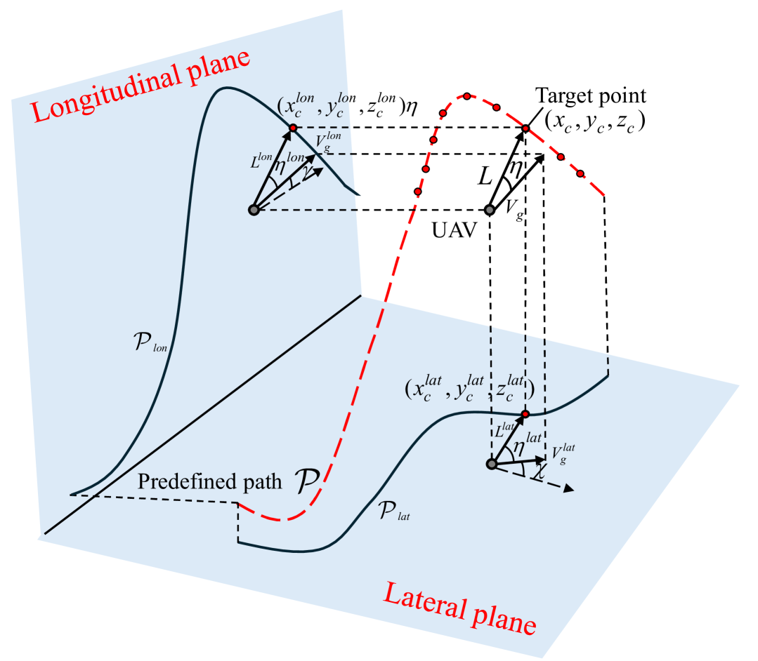
Figure 1: The schematic diagram of look-ahead pursuit guidance law decoupled along the longitudinal plane and lateral plane projections for a predefined path

and the virtual target point $P_{c}=(x_{c},y_{c},z_{c})$ is defined as the nearest point located ahead along the predefined reference path in the direction of velocity as[14]

$$P_{c}=\underset{(x,y,z)\in\mathcal{P}}{\text{argmin}}|q_{L}V_{g}-\sqrt{(x_{p}-x)^{2}+(y_{p}-y)^{2}+(z_{p}-z)^{2}}|$$ (6)

where $q_{L}$ represents the coefficient that adaptively adjusts the look-ahead length in relation to the UAV’s ground velocity. During the process of tracking a virtual target point, its first-order derivative $\dot{x}_{c},\dot{y}_{c},\dot{z}_{c}$ can be considered as zeros under the condition of not considering abrupt target switching. Meanwhile the longitudinal and lateral acceleration commands $a_{yc}$ and $a_{zc}$ can be organized as

$$\begin{cases}\begin{split}a_{yc}&=k_{q}V_{g}\sin\eta^{lat}\cos\gamma\\ a_{zc}&=k_{q}V_{g}\sin\eta^{lon}+g\cos\gamma\end{split}\end{cases}$$ (7)

where its lateral look-ahead angle $\eta^{lat}$ and longitudinal look-ahead angle $\eta^{lon}$ can be rewritten as

$$\begin{cases}\begin{split}\eta^{lat}&=\tan^{-1}\frac{y_{c}-y_{p}}{x_{c}-x_{p}}-\chi\\ \eta^{lon}&=\tan^{-1}\frac{z_{c}-z_{p}}{\sqrt{(x_{c}-x_{p})^{2}+(y_{c}-y_{p})^{2}}}-\gamma\end{split}\end{cases}$$ (8)

and $\eta^{lat}$ is limited to $\eta^{lat}_{\min}\leq\eta^{lat}\leq\eta^{lat}_{\max}$, $\eta^{lon}$ is limited to $\eta^{lon}_{\min}\leq\eta^{lon}\leq\eta^{lon}_{\max}$, $k_{q}$ is the gain ratio both in longitudinal and lateral planes.

Specifically, it is precisely because when $\eta^{lat}$ and $\eta^{lon}$ both are zero, the velocity direction of the UAV can be ensured to be coincide with the LOS, stablizing the positional errors $e_{x}$, $e_{y}$, and $e_{z}$ to zeros in a finite time. This is the foundational principle of look-ahead pursuit control, which will be further elucidated by the following theorem.

Theorem 1.

The $e_{x}$, $e_{y}$, and $e_{z}$ will be stablized to 0 within a finite time $T(e_{0})\leq\sqrt{e^{2}_{x}(0)+e^{2}_{y}(0)+e^{2}_{z}(0)}/V_{g}$ under the initial position error $e_{x}(0),e_{y}(0),e_{z}(0)$ if $\eta^{lat}=0$,$\eta^{lon}=0$.

Proof.

According to the $\eta^{lat}=0$,$\eta^{lon}=0$, there exists

$$\begin{cases}\begin{split}\sin\chi&=\frac{y_{c}-y_{p}}{\sqrt{(x_{c}-x_{p})^{2}+(y_{c}-y_{p})^{2}}}\\ \cos\chi&=\frac{x_{c}-x_{p}}{\sqrt{(x_{c}-x_{p})^{2}+(y_{c}-y_{p})^{2}}}\\ \sin\gamma&=\frac{z_{c}-z_{p}}{\sqrt{(x_{c}-x_{p})^{2}+(y_{c}-y_{p})^{2}+(z_{c}-z_{p})^{2}}}\\ \cos\gamma&=\frac{\sqrt{(x_{c}-x_{p})^{2}+(y_{c}-y_{p})^{2}}}{\sqrt{(x_{c}-x_{p})^{2}+(y_{c}-y_{p})^{2}+(z_{c}-z_{p})^{2}}}\end{split}\end{cases}$$

and $\dot{x}_{p}=-e_{x}$, $\dot{y}_{p}=-e_{y}$, $\dot{x}_{p}=-e_{y}$. Substitute it into Eq.(1) to obtain:

$$\begin{cases}\begin{split}\dot{e}_{x}=-V_{g}\frac{e_{x}}{\sqrt{e_{x}^{2}+e_{y}^{2}+e_{z}^{2}}}\\ \dot{e}_{y}=-V_{g}\frac{e_{y}}{\sqrt{e_{x}^{2}+e_{y}^{2}+e_{z}^{2}}}\\ \dot{e}_{z}=-V_{g}\frac{e_{z}}{\sqrt{e_{x}^{2}+e_{y}^{2}+e_{z}^{2}}}\\ \end{split}\end{cases}$$

we can construct lyapunov function $V(e)=\frac{a}{2}(e_{x}^{2}+e_{y}^{2}+e_{z}^{2}),a>0$, there exists

$$\begin{split}\dot{V}(e)&=a(e_{x}\dot{e}_{x}+e_{y}\dot{e}_{y}+e_{z}\dot{e}_{z})\\ &=-aV_{g}\sqrt{e_{x}^{2}+e_{y}^{2}+e_{z}^{2}}\\ &=-\sqrt{2a}V_{g}V(e)^{\frac{1}{2}}\end{split}$$

Hence, the settling time is:

$$T(e_{0})\leq\frac{V(e_{0})^{\frac{1}{2}}}{\sqrt{2a}V_{g}(1-\frac{1}{2})}=\frac{\sqrt{e^{2}_{x}(0)+e^{2}_{y}(0)+e^{2}_{z}(0)}}{V_{g}}$$

∎

Meanwhile,Eq.(7) can guarantee the exponential convergence of the kinematic model Eq.(1). We substitute Eq.(7) and Eq.(8) into Eq.(2) to obtain:

$$\begin{cases}\begin{split}\dot{\chi}&=k_{q}\sin(\tan^{-1}\frac{y_{c}-y_{p}}{x_{c}-x_{p}}-\chi)+d_{\chi}\\ \dot{\gamma}&=k_{q}\sin(\tan^{-1}\frac{z_{c}-z_{p}}{\sqrt{(x_{c}-x_{p})^{2}+(y_{c}-y_{p})^{2}}}-\gamma)+d_{\gamma}\end{split}\end{cases}$$ (9)

We can directly solve the ordinary differential Eq.(9) when the disturbances $d_{\gamma},d_{\chi}=0$ from initial time $t_{0}$ to $t$ that

$$\begin{cases}\begin{split}|\eta^{lat}(t)|&\leq 2|\tan\frac{\eta^{lat}(t_{0})}{2}|\exp(-k_{q}(t-t_{0}))\\ |\eta^{lon}(t)|&\leq 2|\tan\frac{\eta^{lon}(t_{0})}{2}|\exp(-k_{q}(t-t_{0}))\\ \end{split}\end{cases}$$ (10)

The aforementioned conclusion indicates that the disturbance-free guidance law designed for the path angle can guarantee exponential stabilization of the look-ahead angle errors, thereby ensuring stabilization of the positional errors.

III-A Robust stability of longitudinal-lateral guidance law

Here we will consider a guidance law with high robustness under the condition where the disturbances $d_{\gamma}$ and $d_{\chi}$ are not equal to zeros. To better describe the controller under disturbance conditions, we introduce the concept of robust stability.

Definition 1.

(Robust stability) For perturbed nonlinear system $\dot{y}=f(t,y)+g(t,y)$, $y\in\mathbb{R}^{n}$,$f(t,0)=0$, $f,g\in C[I\times S_{H},\mathbb{R}^{n}]$,$S_{H}=\{x|||x||\leq H\}$, if $\forall\varepsilon>0$, there exists $\delta_{1}(\varepsilon)>0$ and $\delta_{2}(\varepsilon)>0$ to make $||g(t,y)||\leq\delta_{1}(\varepsilon)$, $||y(0)||\leq\delta_{2}(\varepsilon)$, then the trivial solution of $\dot{y}=f(t,y)+g(t,y),f(t,0)=0$ exhibits robust stability.

The definition of robust stability characterizes a property such that for any perturbed system, the perturbed solution can be kept within an arbitrarily small range by adjusting the restricted range of the perturbation $g(t,y)$ and the initial values of trivial solution $y(0)$. The following lemma provides the basis for judging the robust stability of a perturbed system.

Lemma 1.

(T.Yoshizawa[22]) If for a nonlinear system $\dot{x}=f(t,x)$,$x\in S_{H}$,$f(t,0)=0$, there exists a corresponding lyapunov function $V(t,x)\in[I\times S_{H},\mathbb{R}_{+}^{1}]$ that satisfies the following conditions:

• $\alpha(||x||)\leq V(t,x)\leq\beta(||x||)$ involving non-decreasing nonnegative functions $\alpha,\beta:C[\mathbb{R}^{1}_{+}\cup\{0\},\mathbb{R}^{1}_{+}\cup\{0\}]$, both of which are zeros only at the origin;

• $\dot{V}(t,x)|\leq-cV(t,x),c>0$;

• $|V(t,x_{1})-V(t,x_{2})|\leq K||x-y||,\forall x_{1},x_{2}\in S_{H}$;

then the trivial solution of perturbed nonlinear system exhibits robust stability.

Lemma 1 reveals a fact that, in a certain sense, a lyapunov function under constrained exponential stability often implies a certain degree of robust stability. The following theorem demonstrates that the look-ahead pursuit control possesses robust stability when the look-ahead angle is within a certain range.

Theorem 2.

If there exists $0<\delta<\frac{\pi}{2}$ such that

$$|\eta^{lat}|\leq\delta,|\eta^{lon}|\leq\delta$$ (11)

for any $t$ holds, the perturbed kinematic model Eq.(2) will exhibit robust stability under the guidance law Eq.(7).

Proof.

Eq.(9) can be transformed into

$$\begin{cases}\begin{split}\dot{\eta^{lat}}&=-k_{q}\sin(\eta^{lat})+\dot{C}_{1}-d_{\chi}\\ \dot{\eta^{lon}}&=-k_{q}\sin(\eta^{lon})+\dot{C}_{2}-d_{\gamma}\end{split}\end{cases}$$ (12)

where

$$\begin{cases}\begin{split}C_{1}&=\tan^{-1}\frac{y_{c}-y_{p}}{x_{c}-x_{p}}\\ C_{2}&=\tan^{-1}\frac{z_{c}-z_{p}}{\sqrt{(x_{c}-x_{p})^{2}+(y_{c}-y_{p})^{2}}}\end{split}\end{cases}$$ (13)

We construct a positive define lyapunov function $V(\eta^{lon},\eta^{lat})=a\sin^{2}\eta^{lon}+a\sin^{2}\eta^{lat}$,$a>0$ for the unperturbed model

$$\begin{cases}\begin{split}\dot{\eta^{lat}}&=-k_{q}\sin(\eta^{lat})\\ \dot{\eta^{lon}}&=-k_{q}\sin(\eta^{lon})\end{split}\end{cases}$$

$$\frac{4a}{\pi^{2}}((\eta^{lon})^{2}+(\eta^{lat})^{2})\leq V(\eta^{lon},\eta^{lat})\leq a((\eta^{lon})^{2}+(\eta^{lat})^{2})$$

It is obvious that $V(\eta^{lon},\eta^{lat})$ is lipstichz continuous within $K=2a$, we obtain the following formulation after taking the first-order derivative of $V(\eta^{lon},\eta^{lat})$,

$$\begin{split}\dot{V}(\eta^{lon},\eta^{lat})&=-2a(\sin\eta^{lon}\cos\eta^{lon}\dot{\eta^{lon}}+\sin\eta^{lat}\cos\eta^{lat}\dot{\eta^{lat}})\\ &=-2ak_{q}(\sin^{2}\eta^{lon}\cos\eta^{lon}+\sin^{2}\eta^{lat}\cos\eta^{lat})\end{split}$$

Meanwhile the $\cos\eta^{lat}$ and $\cos\eta^{lon}$ is limited to

$$0<\cos\delta\leq\cos\eta^{lat}\leq 1,0<\cos\delta\leq\cos\eta^{lon}\leq 1$$

Hence,

$$\begin{split}\dot{V}(\eta^{lon},\eta^{lat})&\leq-2ak_{q}\cos\delta(\sin^{2}\eta^{lon}+\sin^{2}\eta^{lat})\\ &=-2k_{q}\cos\delta V(\eta^{lon},\eta^{lat})\end{split}$$

Thereby all conditions are satisfied. ∎

The aforementioned theorem delineates that under condition Eq.(11), as well as with certain appropriate disturbances and initial values, the system retains a certain degree of robustness, enabling $\eta^{lon}$ and $\eta^{lat}$ to still converge exponentially to zero. The following delineates a relatively conservative region of attraction as

$$\begin{split}||y(t_{0})||\leq\frac{\pi}{2}\sqrt{\frac{\sup_{t}||g(t,y(t))||}{k_{q}\cos\delta}}\\ \sup_{t}||g(t,y(t))||\leq\frac{16\varepsilon^{2}k_{q}\cos\delta}{\pi^{4}}\end{split}$$ (14)

for any $||y(t)||<\varepsilon$ within which the perturbed system can maintain robust stability.

III-B Robust compensation term design

Despite the guidance law Eq.(7) exhibiting certain robust performance, as indicated by Eq.(14), when the larger magnitude of the disturbances occur, the guidance law may not guarantee that the $\eta^{lat}$ and $\eta^{lon}$ converge to zero. Therefore, we aim to incorporate a compensation term $f_{lat}$, $f_{lon}$ into the existing guidance law as Eq.(15), enabling rapid stabilization of $\eta^{lat}$ and $\eta^{lon}$ within a finite time for any bounded disturbance $d_{\gamma}$ and $d_{\chi}$.

$$\begin{cases}\begin{split}a_{yc}^{*}&=(k_{q}\sin\eta^{lat}+f_{lat})V_{g}\cos\gamma\\ a_{zc}^{*}&=(k_{q}\sin\eta^{lon}+f_{lon})V_{g}+g\cos\gamma\end{split}\end{cases}$$ (15)

For this purpose, we first introduce the following lemma.

Lemma 2.

For given perturbed system as

$$\begin{cases}\begin{split}\dot{e}_{\chi}&=-k_{q}\sin e_{\chi}+f_{\chi}+d_{\chi}\\ \dot{e}_{\gamma}&=-k_{q}\sin e_{\gamma}+f_{\gamma}+d_{\gamma}\end{split}\end{cases}$$ (16)

where $d=(d_{\chi},d_{\gamma})^{T}$ represent the disturbance terms, $||d||_{2}\leq L_{d}$, $f_{\chi}$ and $f_{\gamma}$ denote the compensation term. If there exists a $\tau>0$ to make:

$$\begin{split}\frac{f_{\chi}\sin e_{\chi}\cos e_{\chi}+f_{\gamma}\sin e_{\gamma}\cos e_{\gamma}}{\sqrt{\sin^{2}e_{\chi}\cos^{2}e_{\chi}+\sin^{2}e_{\gamma}\cos^{2}e_{\gamma}}}+L_{d}+\tau\leq 0\end{split}$$ (17)

where

$$|e_{\gamma}|\leq\delta<\frac{\pi}{2},|e_{\chi}|\leq\delta<\frac{\pi}{2}$$ (18)

then the origin of above perturbed system is fast finite-time stable, and the settling time, depending on the initial state $e_{\gamma}(0)$, $e_{\chi}(0)$ is given by

$$T(e_{0})\leq\frac{1}{k_{q}\cos\delta}\ln(1+\frac{k_{q}\sqrt{\sin^{2}e_{\gamma}(0)+\sin^{2}e_{\chi}(0)}}{\tau})$$ (19)

Proof.

We construct a positive define lyapunov function $V(e)=a\sin^{2}e_{\chi}+a\sin^{2}e_{\gamma}$,$a>0$ for the perturbed model Eq.(16) to obtain

$$\begin{split}\dot{V}(e)&=2a(\sin e_{\chi}\cos e_{\chi}\dot{e}_{\chi}+\sin e_{\gamma}\cos e_{\gamma}\dot{e}_{\gamma})\\ &=2a(\sin e_{\chi}\cos e_{\chi}(-k_{q}\sin e_{\chi}+f_{\chi}+d_{\chi})\\ &+\sin e_{\gamma}\cos e_{\gamma}(-k_{q}\sin e_{\gamma}+f_{\gamma}+d_{\gamma}))\\ &\leq-2k_{q}\cos\delta(a\sin^{2}e_{\chi}+a\sin^{2}e_{\gamma})\\ &+2a(\sin e_{\chi}\cos e_{\chi}d_{\chi}+\sin e_{\gamma}\cos e_{\gamma}d_{\gamma})\\ &+2a(f_{\chi}\sin e_{\chi}\cos e_{\chi}+f_{\gamma}\sin e_{\gamma}\cos e_{\gamma})\\ &\leq+2aL_{d}\sqrt{(\sin e_{\chi}\cos e_{\chi})^{2}+(\sin e_{\gamma}\cos e_{\gamma})^{2}}\\ &+2a(f_{\chi}\sin e_{\chi}\cos e_{\chi}+f_{\gamma}\sin e_{\gamma}\cos e_{\gamma})-2k_{q}\cos\delta V(e)\\ &\leq-2k_{q}\cos\delta V(e)\\ &-2a\tau\sqrt{(\sin e_{\chi}\cos e_{\chi})^{2}+(\sin e_{\gamma}\cos e_{\gamma})^{2}}\\ &\leq-2k_{q}\cos\delta V(e)-2\tau\sqrt{a}\cos\delta V(e)^{\frac{1}{2}}\end{split}$$

The above derivation leads to the following conclusion,

$$\dot{V}(e)+2k_{q}\cos\delta V(e)+2\tau\sqrt{a}\cos\delta V(e)^{\frac{1}{2}}\leq 0$$

Hence the origin of above perturbed system is fast finite-time stable, and settling time bound is Eq.(19). ∎

In the following theorem, we will present the form of the compensation term $f_{lat}$ and $f_{lon}$ that enables the perturbed system Eq.(2) to achieve fast stabilization in a finite time.

Theorem 3.

The perturbed system Eq.(2) will be fast stabilizd in a finite time if the following compensation terms is adopted into modified guidance law Eq.(15),

$$\begin{cases}f_{lat}&=\dot{C}_{1}-f_{\chi}\\ f_{lon}&=\dot{C}_{2}-f_{\gamma}\end{cases}$$ (20)

where there exists a $\tau>0$ such that

$$\begin{split}\frac{f_{\chi}\sin\eta^{lat}\cos\eta^{lat}+f_{\gamma}\sin\eta^{lon}\cos\eta^{lon}}{\sqrt{\sin^{2}\eta^{lat}\cos^{2}\eta^{lat}+\sin^{2}\eta^{lon}\cos^{2}\eta^{lon}}}+L_{d}+\tau\leq 0\end{split}$$ (21)

$$|\eta^{lon}|\leq\delta<\frac{\pi}{2},|\eta^{lat}|\leq\delta<\frac{\pi}{2}$$ (22)

And the settling time bound is given by

$$T(\eta^{lon},\eta^{lat})\leq\frac{1}{k_{q}\cos\delta}\ln(1+\frac{k_{q}}{\tau}\sqrt{\sin^{2}\eta^{lon}+\sin^{2}\eta^{lat}})$$ (23)

Proof.

Eq.(2) can be transformed into following formulations by substituting compensation terms Eq.(20) and guidance law Eq.(15).

$$\begin{cases}\begin{split}\dot{\eta}^{lat}&=-k_{q}\sin\eta^{lat}+f_{\chi}-d_{\chi}\\ \dot{\eta}^{lon}&=-k_{q}\sin\eta^{lon}+f_{\gamma}-d_{\gamma}\end{split}\end{cases}$$

According to Lemma 2, the $\eta^{lon}$ and $\eta^{lat}$ is fast stablized to zeros in finite time. ∎

To confine $a_{yc}^{*}$ and $a_{zc}^{*}$ within the range specified in Eq.(4), it is necessary to control the bounds of $f_{lat}$ and $f_{lon}$ as follows:

$$f_{lat}^{\min}\leq f_{lat}\leq f_{lat}^{\max},f_{lon}^{\min}\leq f_{lon}\leq f_{lon}^{\max}$$ (24)

$$\begin{split}f_{\chi}^{\min}\leq f_{\chi}\leq f_{\chi}^{\max},f_{\gamma}^{\min}\leq f_{\gamma}\leq f_{\gamma}^{\max}\end{split}$$ (25)

where

$$\begin{cases}\begin{split}f_{\chi}^{\min}&=\dot{C}_{1}-f_{lat}^{\max},f_{\chi}^{\max}=\dot{C}_{1}-f_{lat}^{\min}\\ f_{\gamma}^{\min}&=\dot{C}_{2}-f_{lon}^{\max},f_{\gamma}^{\max}=\dot{C}_{2}-f_{lon}^{\min}\end{split}\end{cases}$$ (26)

$$\begin{cases}\begin{split}&f_{lat}^{\min}=\frac{a_{yc}^{\min}}{V_{g}\cos\gamma}-k_{q}\sin\eta^{lat}\\ &f_{lat}^{\max}=\frac{a_{yc}^{\max}}{V_{g}\cos\gamma}-k_{q}\sin\eta^{lat}\\ &f_{lon}^{\min}=\frac{a_{zc}^{\min}-g\cos\gamma-k_{q}\sin\eta^{lon}V_{g}}{V_{g}}\\ &f_{lon}^{\max}=\frac{a_{zc}^{\max}-g\cos\gamma-k_{q}\sin\eta^{lon}V_{g}}{V_{g}}\end{split}\end{cases}$$ (27)

To satisfy the longitudinal and lateral acceleration constraints of the compensation term, it is necessary to impose the following amplitude limitations on the modified guidance law Eq.(15) as

$$\begin{cases}\begin{split}\hat{f}_{lat}&={clip}(f_{lat},f_{lat}^{\min},f_{lat}^{\max})\\ \hat{f}_{lon}&={clip}(f_{lon},f_{lon}^{\min},f_{lon}^{\max})\end{split}\end{cases}$$ (28)

The formula used to modify the guidance law after compensation is as follows:

$$\begin{cases}\begin{split}a_{yc}^{*}&=a_{yc}+V_{g}\cos\gamma\hat{f}_{lat}\\ a_{zc}^{*}&=a_{zc}+V_{g}\hat{f}_{lon}\end{split}\end{cases}$$ (29)

IV Optimal Look-ahead Pursuit Controller design

In this section, we will design an adaptive longitudinal-lateral look-ahead pursuit controller by selecting optimal $f_{\chi}$ and $f_{\gamma}$ based on the current states and the constrains to achieve robust control. The optimal solution problem for the compensation amount can be transformed into a targeted linear programming(LP) problem for solving different look-ahead angle scenarios.

Figure 2: Robust longitudinal and lateral look-ahead pursuit path following guidance law in the presence of constrained disturbance

IV-A Selection of virtual target point for optimization

For the virtual target point $P_{c}$ located on the reference path $\mathcal{P}$ that necessitates tracking, the satisfaction of condition Eq.(22) is essential to ensure both robust stability and finite-time stability. This implies that the current virtual path point needs to be positioned as closely as feasible along the velocity forward direction of the current location point, while simultaneously ensuring that robustness constraints are met. In addition, the proximity of the flight time from the current location point $P_{g}=(x_{g},y_{g},z_{g})$ to the virtual target point $P_{c}=(x_{c},y_{c},z_{c})$ should not be excessively short, as an overly short flight duration in such scenarios may hinder the timely elimination of deviations $\eta^{lon}$ and $\eta^{lat}$. Here, the upper bound of $T(P_{c})$ can be estimated by

$$T(P_{c})=\frac{1}{k_{q}\cos\delta}\ln(1+\frac{k_{q}}{\hat{\tau}}\sqrt{\sin^{2}\eta^{lon}+\sin^{2}\eta^{lat}})$$ (30)

To simplify calculations, $\hat{\tau}$ can be approximately valued within the range of 0.5 to 2. In summary, we aim to select the point closest to the current location point from the following set $C$ as the virtual target point

$$C=\{P_{c}\in\mathcal{P}||\eta^{lon}|\leq\delta,|\eta^{lat}|\leq\delta,||P_{c}-P_{g}||_{2}\geq V_{g}T(P_{c})\}$$ (31)

IV-B Achieving the optimal solution for $f_{\chi}$ and $f_{\gamma}$

The optimal objective is to minimize upper bound of the time required for finite stable as

$$\begin{split}&\underset{f_{\chi},f_{\gamma},k_{q}}{\min}Eq.(\ref{equ:settling time 2})\\ s.t.\quad&Eq.(\ref{equ:compensation term 2}),Eq.(\ref{equ:constrain 2}),Eq.(\ref{equ:f_gamma_chi_sat})\end{split}$$ (32)

In the optimization problem Eq.(32), the feasible region for the compensatory terms $(f_{\gamma}^{*},f_{\chi}^{*})$ that guarantees finite-time stablization is characterized as the deep blue area depicted in Fig.(3). This area is formed by the intersection of the boundaries of $f_{\gamma}$ and $f_{\chi}$, outlined by the rectangular boxes, with the inequality region of Eq.(21) that excludes the origin. In the coordinate system of compensation quantities $f_{\chi}$ and $f_{\gamma}$ as shown in Fig.(3), the intercepts $I_{\chi}$, $I_{\gamma}$ on the horizontal and vertical axes formed by the linear equation in Eq.(21) along with $f_{\chi}$ and $f_{\gamma}$ can be respectively described as

$$I_{\chi}=-\frac{L_{d}+\tau}{\sin\theta},I_{\gamma}=-\frac{L_{d}+\tau}{\cos\theta}$$ (33)

where

$$\begin{cases}\begin{split}\sin\theta&=\frac{\sin\eta^{lat}\cos\eta^{lat}}{\sqrt{\sin^{2}\eta^{lat}\cos^{2}\eta^{lat}+\sin^{2}\eta^{lon}\cos^{2}\eta^{lon}}}\\ \cos\theta&=\frac{\sin\eta^{lon}\cos\eta^{lon}}{\sqrt{\sin^{2}\eta^{lat}\cos^{2}\eta^{lat}+\sin^{2}\eta^{lon}\cos^{2}\eta^{lon}}}\end{split}\end{cases}$$ (34)

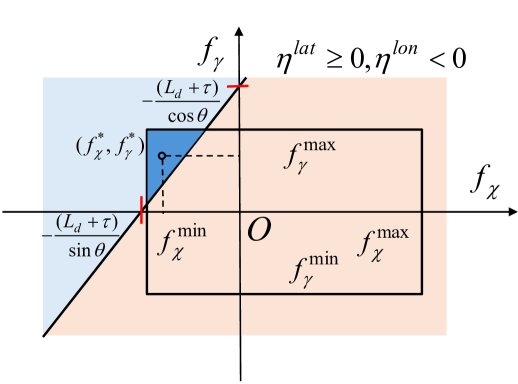
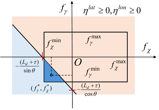
(a)	(b)
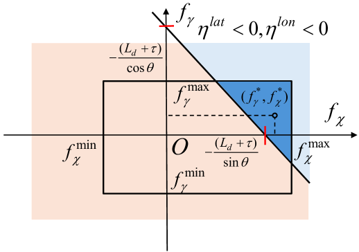
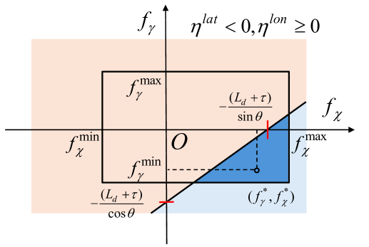
(c)	(d)

Figure 3: The schematic diagram provided to illustrate the feasible region at various look-ahead angles $\eta^{lon}$ and $\eta^{lat}$, where the feasible region is displayed as a deep blue area, located at the intersection within the rectangular frame and the light blue area, while the orange area and light blue area depict their infeasible ranges. (a): $\eta^{lat}\geq 0,\eta^{lon}<0$; (b): $\eta^{lat}\geq 0,\eta^{lon}\geq 0$; (c): $\eta^{lat}<0,\eta^{lon}<0$; (d): $\eta^{lat}<0,\eta^{lon}\geq 0$.

In the case where the feasible region is non-empty, the optimization objective in Eq.(32) can be transformed into maximizing the $\tau$, which corresponds to maximizing the distance of the horizontal and vertical intercepts $I_{\gamma}$ and $I_{\chi}$ of the line away from the origin. It is evident that such an optimal solution is achieved precisely at the vertices of the rectangular bounding box. Assuming that the optimal solution is denoted as $(f_{\chi}^{opt},f_{\gamma}^{opt})$, the necessary and sufficient condition for the existence of the feasible region can be determined by

$$\frac{f_{\chi}^{opt}\sin\eta^{lat}\cos\eta^{lat}+f_{\gamma}^{opt}\sin\eta^{lon}\cos\eta^{lon}}{\sqrt{\sin^{2}\eta^{lat}\cos^{2}\eta^{lat}+\sin^{2}\eta^{lon}\cos^{2}\eta^{lon}}}+L_{d}<0$$ (35)

A typical selection of $f_{\gamma}$ and $f_{\chi}$ based on the aforementioned feasible region can be described as:

$$\begin{cases}\begin{split}f_{\chi}^{*}&=-\frac{k_{1}\sqrt{\sin^{2}\eta^{lat}\cos^{2}\eta^{lat}+\sin^{2}\eta^{lon}\cos^{2}\eta^{lon}}}{\sin\eta^{lat}\cos\eta^{lat}}\\ f_{\gamma}^{*}&=-\frac{k_{2}\sqrt{\sin^{2}\eta^{lat}\cos^{2}\eta^{lat}+\sin^{2}\eta^{lon}\cos^{2}\eta^{lon}}}{\sin\eta^{lon}\cos\eta^{lon}}\\ \end{split}\end{cases}$$ (36)

where $k_{1}$ and $k_{2}$ represent the parameters that need to be optimized, and the inequality $k_{1}+k_{2}>L_{d}$ ensures the achievement of fast finite-time stability. However, if the feasible region is empty, there needs to readjust the $k_{q}$ to shift the position of the bounding box and thereby attempt to construct a suitable feasible region. Additionally, we endeavor to ensure that $k_{q}$ follows a decremental search principle, as excessively small $k_{q}$ may result in larger finite stable time.

IV-C Online convex optimization for $k_{1}$ and $k_{2}$

While we aim to obtain the fastest stabilization time by optimizing Eq.(32), excessively rapid stabilization is not necessary as it can lead to repeated oscillations during the error convergence process. In contrast, we prefer to minimize the positive definite quadratic form of input accelerations, as this approach typically implies lower input energy consumption, thereby relatively reducing the frequency of error oscillations. When Eq.(36) is adopted as the specific form of the compensation term to be optimized, we can obtain the explicit expression for the input accelerations $u=(a_{yc}^{*},a_{zc}^{*})^{T}$ by substituting Eq.(36), Eq.(34) into Eq.(29), yielding:

$$\small\begin{bmatrix}a_{yc}^{*}\\ a_{zc}^{*}\end{bmatrix}=\begin{bmatrix}(k_{q}\sin\eta^{lat}+\dot{C}_{1})V_{g}\cos\gamma\\ (k_{q}\sin\eta^{lon}+\dot{C}_{2})V_{g}+g\cos\gamma\end{bmatrix}\\ +\begin{bmatrix}\frac{V_{g}\cos\gamma}{\sin\theta}&0\\ 0&\frac{V_{g}}{\cos\theta}\end{bmatrix}\begin{bmatrix}k_{1}\\ k_{2}\end{bmatrix}$$ (37)

Assuming the continuity of $\dot{C}_{1}$ and $\dot{C}_{2}$, it can be numerically approximated using the difference method as follows:

$$\dot{C}_{1}(t)\approx\frac{C_{1}(t)-C_{1}(t-\Delta t)}{\Delta t},\dot{C}_{2}(t)\approx\frac{C_{2}(t)-C_{2}(t-\Delta t)}{\Delta t}$$ (38)

We denote $k=(k_{1},k_{2})^{T}$, and the above equation can then be transformed into

$$u=b+Ak$$ (39)

where

$$b=\begin{bmatrix}(k_{q}\sin\eta^{lat}+\dot{C}_{1})V_{g}\cos\gamma\\ (k_{q}\sin\eta^{lon}+\dot{C}_{2})V_{g}+g\cos\gamma\end{bmatrix},A=\begin{bmatrix}\frac{V_{g}\cos\gamma}{\sin\theta}&0\\ 0&\frac{V_{g}}{\cos\theta}\end{bmatrix}$$ (40)

Based on the input constraint given by Eq.(4), we can derive the upper and lower bounds for $k$, denoted as

$$u_{\min}-b\leq Ak\leq u_{\max}-b$$ (41)

where $u_{\min}=(a_{yc}^{\min},a_{zc}^{\min})^{T}$, $u_{\max}=(a_{yc}^{\max},a_{zc}^{\max})^{T}$. To prevent large oscillations in the input $u$, it is necessary to impose constraints on its derivative during each iteration of the optimization process as

$$\dot{u}_{\min}\leq\dot{u}\leq\dot{u}_{\max}$$ (42)

which can be discretized by implementing an estimation of $\Delta u\approx\dot{u}\Delta t$ to obtain

$$\dot{u}_{\min}\Delta t-\Delta b\leq\Delta Ak\leq\dot{u}_{\max}\Delta t-\Delta b$$ (43)

For a given positive definite matrix $R=R^{T}>0$, in order to minimize the energy increment of the input accelerations represented by $\frac{1}{2}\Delta u^{T}R\Delta u$, the optimization problem for the coefficients $k$, under the existence of its feasible region, can be transformed into the following online convex optimization problem as

$$\begin{split}&\underset{k}{\min}\frac{1}{2}k^{T}\Delta A^{T}R\Delta Ak+\Delta b^{T}R\Delta Ak\\ s.t.&\begin{bmatrix}&A&\\ &-A&\\ &\Delta A&\\ &-\Delta A&\\ &-1,-1&\end{bmatrix}k\leq\begin{bmatrix}u_{\max}-b\\ b-u_{\min}\\ \dot{u}_{\max}\Delta t-\Delta b\\ \Delta b-\dot{u}_{\min}\Delta t\\ -(1+\varepsilon)L_{d}\end{bmatrix}\end{split}$$ (44)

where $\varepsilon>0$ serves as a predetermined threshold for disturbance rejection, which can be efficiently tackled in real-time by employing the interior point method.

V Simulation

In this section, we conduct a comprehensive analysis of the path - following performance of the Robust Longitudinal and Lateral Look-ahead Pursuit(RLLP) guidance law. The analysis is carried out under the conditions of bounded white - noise disturbances and practical non-smooth predefined paths. Additionally, by incorporating optimal compensation terms, we have further enhanced numerous critical performance aspects.

V-A Performance of Robust Look-ahead Pursuit Controller

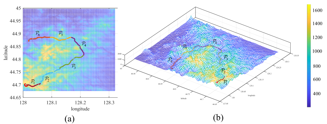
Figure 4: Top view and side view of a six-segment complex non-smooth low-altitude path used for path-following experiments. (a): Top view; (b): Side view.

In order to demonstrate the path-following performance of the proposed algorithm on multiple different non-smooth paths, we carry out comparative path-following experiments with white-noise disturbances for each of the six path segments $\mathcal{P}_{1},\mathcal{P}_{2},...\mathcal{P}_{6}$ as shown in Fig.4, where the disturbance is regulated to mimic uniformly distributed random white noise, characterized by a mean value of 0 and a standard deviation of $\frac{L_{d}}{\sqrt{2}}$, expressed as

$$d_{\chi},d_{\gamma}\sim U(0,\frac{L_{d}}{\sqrt{2}})$$ (45)

For further clarification, we set the weight matrix $R=\begin{pmatrix}0.1&0\\ 0&0.1\end{pmatrix}$, the controller’s sampling time to $\Delta t=0.1s$, the period of the disturbances to $5\Delta t=0.5s$, the aircraft’s constant flight velocity to $V_{g}=25m/s$, the acceleration boundary values to $a_{yc}^{\max}=25m/s^{2}$, $a_{yc}^{\min}=-25m/s^{2}$, $a_{zc}^{\max}=14.12m/s^{2}$, $a_{zc}^{\min}=-14.12m/s^{2}$. We compared the path-following performance of the RLLP guidance law under both undisturbed ($L_{d}=0$) and disturbed ($L_{d}=\frac{\pi}{15}$, representing a significant disturbance in practical scenarios) conditions, as illustrated in Fig.5 and Fig.6. Taking the path following results of $\mathcal{P}_{1}$ as an example, the convergence profiles of $\eta^{lon}$ and $\eta^{lat}$ are depicted in Fig.7, and the control-command curves of $a_{yc}$ and $a_{zc}$ are presented in Fig.8.

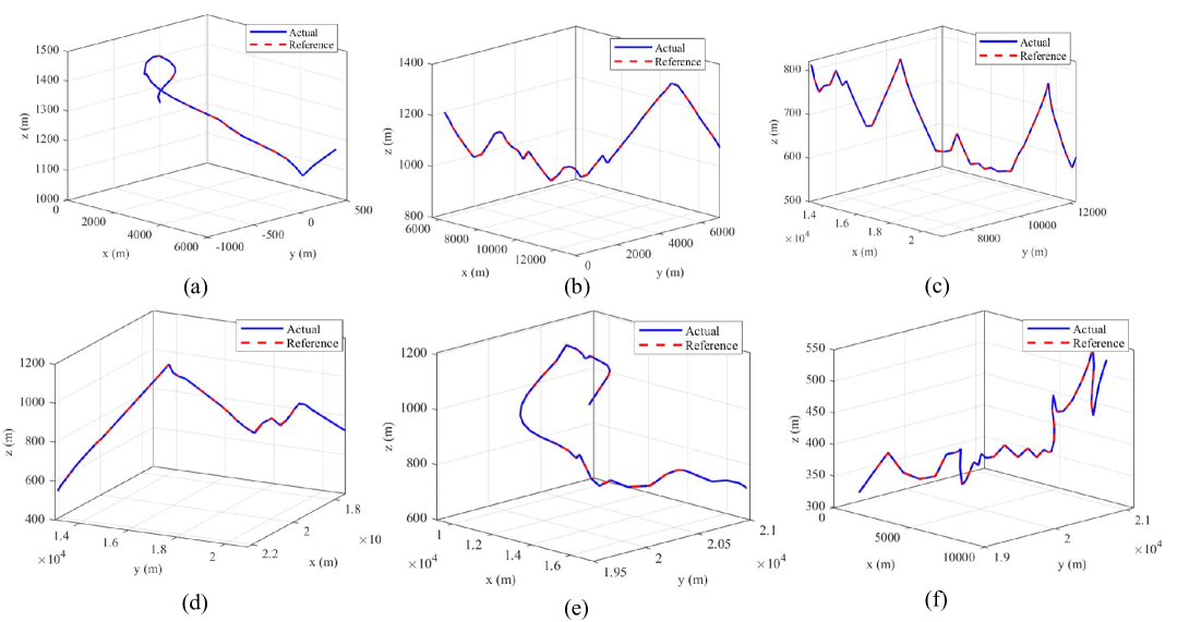
Figure 5: The path-following profiles for $\mathcal{P}_{1}$,$\mathcal{P}_{2}$,$\mathcal{P}_{3}$,$\mathcal{P}_{4}$,$\mathcal{P}_{5}$,$\mathcal{P}_{6}$, corresponding to the robust longitudinal and lateral look-ahead pursuit guidance law when $L_{d}=0$. (a):$\mathcal{P}_{1}$;(b):$\mathcal{P}_{2}$;(c):$\mathcal{P}_{3}$;(d):$\mathcal{P}_{4}$;(e):$\mathcal{P}_{5}$;(f):$\mathcal{P}_{6}$

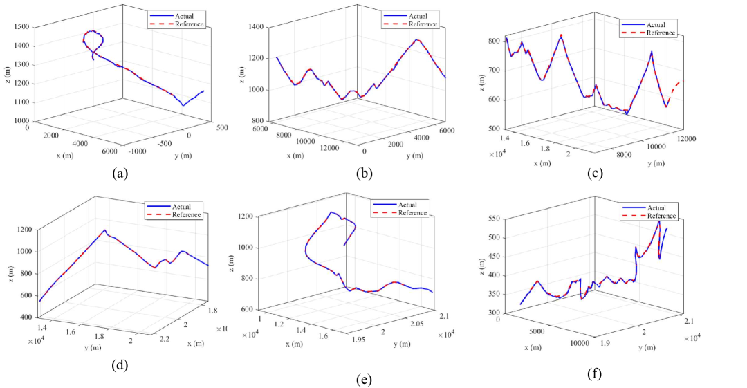
Figure 6: The path-following profiles for $\mathcal{P}_{1}$,$\mathcal{P}_{2}$,$\mathcal{P}_{3}$,$\mathcal{P}_{4}$,$\mathcal{P}_{5}$,$\mathcal{P}_{6}$, corresponding to the robust longitudinal and lateral look-ahead pursuit guidance law when $L_{d}=\frac{\pi}{15}$. (a):$\mathcal{P}_{1}$;(b):$\mathcal{P}_{2}$;(c):$\mathcal{P}_{3}$;(d):$\mathcal{P}_{4}$;(e):$\mathcal{P}_{5}$;(f):$\mathcal{P}_{6}$

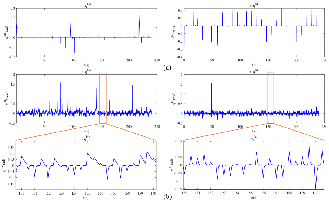
Figure 7: The comparative profiles depicting the changes in $\eta^{lon}$ and $\eta^{lat}$ during the path following process of path $\mathcal{P}_{1}$ under the different conditions of $L_{d}=0$ and $L_{d}=\frac{\pi}{15}$. (a):$L_{d}=0$; (b):$L_{d}=\frac{\pi}{15}$

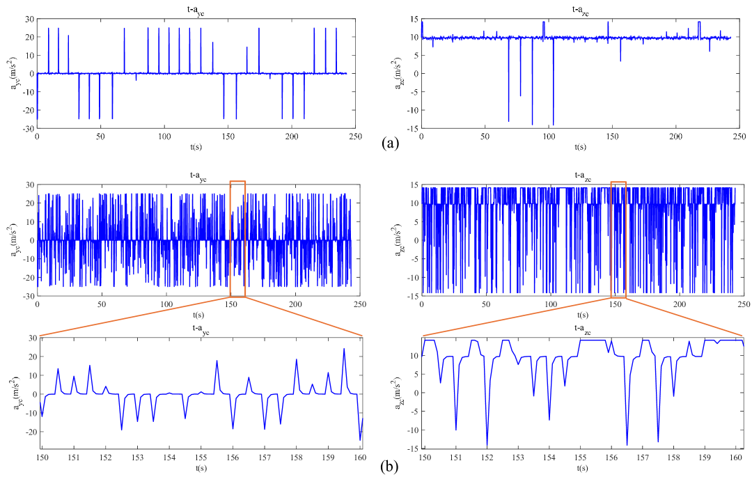
Figure 8: The comparative profiles depicting the changes in $a_{yc}$ and $a_{zc}$ during the path following process of path $\mathcal{P}_{1}$ under the different conditions of $L_{d}=0$ and $L_{d}=\frac{\pi}{15}$. (a):$L_{d}=0$; (b):$L_{d}=\frac{\pi}{15}$.

Specifically, compared to the undisturbed scenario, the RLLP guidance law achieves superior tracking performance across all intended paths to be followed. In the presence of noise disturbances and moving virtual target points, the $\eta^{lon}$ and $\eta^{lat}$ exhibit minimal fluctuations around the origin. Moreover, we quantitatively characterize the oscillation degrees of $\eta^{lon}$ and $\eta^{lat}$, as well as the performance of acceleration $a_{yc}$ and $a_{zc}$ by analyzing their mean values and standard deviations, under different disturbance amplitudes $L_{d}$ as shown in Table I.

TABLE I: Mean values and standard deviations of $\eta^{lon}$, $\eta^{lat}$, $a_{yc}$, $a_{zc}$ profiles for path $\mathcal{P}_{1}$.

$L_{d}$	$\eta^{lon}$	$\eta^{lat}$	$a_{yc}$	$a_{zc}$
0	0.0020 $\pm$ 0.0161	0.0032 $\pm$ 0.0228	0.5141 $\pm$ 3.2695	9.7840 $\pm$ 1.1233
$\frac{\pi}{40}$	0.0111 $\pm$ 0.0252	0.0097 $\pm$ 0.0278	1.9213 $\pm$ 4.6565	9.9673 $\pm$ 3.3427
$\frac{\pi}{30}$	0.0154 $\pm$ 0.0324	0.0124 $\pm$ 0.0423	2.3907 $\pm$ 5.5005	10.2331 $\pm$ 4.0948
$\frac{\pi}{20}$	0.0298 $\pm$ 0.0652	0.0173 $\pm$ 0.0444	3.379 $\pm$ 7.3653	10.8264 $\pm$ 5.4172
$\frac{\pi}{15}$	0.0512 $\pm$ 0.0961	0.0230 $\pm$ 0.0579	4.2776 $\pm$ 8.7193	11.3129 $\pm$ 6.3978
$\frac{\pi}{10}$	0.1231 $\pm$ 0.1983	0.0381 $\pm$ 0.0827	6.1789 $\pm$ 11.0851	11.8918 $\pm$ 7.3803

As $L_{d}$ increases, for $\eta^{lon}$ and $\eta^{lat}$, as well as $a_{yc}$ and $a_{zc}$, both their averages and standard deviations exhibit an approximately linear growth trend. This indicates that the increase in disturbance amplitude affects the control effect of this robust guidance law to some extent. On one hand, a larger disturbance will boost the averages and oscillations of $\eta^{lon}$ and $\eta^{lat}$. On the other hand, it will also result in frequent changes in the acceleration input commands, augmenting the control difficulty and the energy-consumption cost. However, because this robust guidance law always confines the influence of the disturbance within a certain range, the final position-following error remains controlled within a certain range. As shown in Fig.6, a relatively satisfactory following effect is achieved.

V-B Enhanced Performance by Adding Optimal Compensation

To demonstrate the superiority of the convex-optimized RLLP (Optimal RLLP) in addressing the input-command chattering induced by disturbances, a path-following comparative experiment is carried out on path $\mathcal{P}_{1}$ with a perturbation amplitude of $L_{d}=\frac{\pi}{15}$. The Optimal RLLP is compared with the basic RLLP without a compensation term (RLLP) and the RLLP with $k_{1}=k_{2}=0.52$ compensation terms (RLLP with compensation). The objective is to analyze the above method differences across multiple metrics of $\eta^{lon}$, $\eta^{lat}$, $a_{yc}$ and $a_{zc}$. Specifically, the path-following comparison experiments of all algorithms on the perturbed path $\mathcal{P}_{1}$ are shown in Fig.13. Here, we focus on examining the differences among the algorithms when the aircraft is in the descending glide phase during the time period from 150 to 160 seconds. In this stage, the algorithms exhibit relatively similar path-following effects, which is more conducive to conducting a more meticulous comparison of metrics such as the mean and standard deviation of $\eta^{lon}$, $\eta^{lat}$, $a_{yc}$ and $a_{zc}$. As shown in Fig.12, from the perspective of the fluctuation amplitudes of the aforementioned four sequences, we conduct a comprehensive analysis of the performance differences. Obviously, due to the frequent switching of virtual target points and the guarantee of stability within a limited time, the acceleration input commands of the controller and the look-ahead angles are prone to significant fluctuations. However, the Optimal RLLP weakens multiple oscillation peaks by minimizing the input energy as much as possible, as a result of which the optimized curves demonstrate better stability compared with the curves prior to optimization. This performance superiority of the Optimal RLLP algorithm can also be quantitatively measured by the mean and standard deviation. As presented in Fig.11, across multiple dimensions among $\eta^{lon}$, $\eta^{lat}$, $a_{yc}$ and $a_{zc}$, the optimized algorithm shows relatively more stable performance with smaller deviations, whether considering the mean or the standard deviation. Although the application of the compensation term that ensures finite-time stabilization may give rise to excessive oscillations, the minimization of the acceleration increment can effectively compensate for this drawback. This operation ensures that the requirement for the smoothness of the acceleration input commands is satisfied to the greatest extent possible while guaranteeing finite-time stabilization.

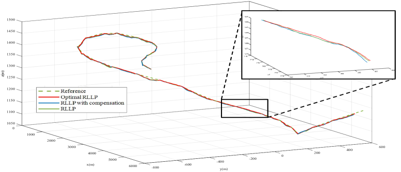
Figure 9: Comparison of path following performance of different algorithms under reference path $\mathcal{P}_{1}$ and disturbance amplitude $L_{d}=\frac{\pi}{15}$.

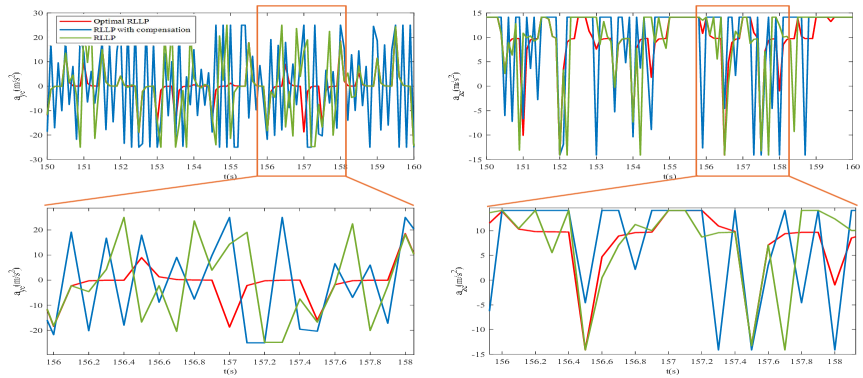
(a)

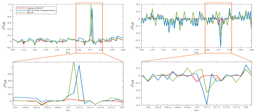
(b)

Figure 10: A comparison of the acceleration commands $a_{yc}$, $a_{zc}$, and the profiles of $\eta^{lon}$ and $\eta^{lat}$ for the RLLP, RLLP with compensation item ($K_{1}=0.52$,$k_{2}=0.52$), and RLLP with optimal compensation item algorithms on path $\mathcal{P}_{1}$ during the time interval of 150s to 160s.

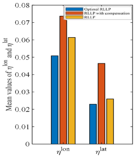
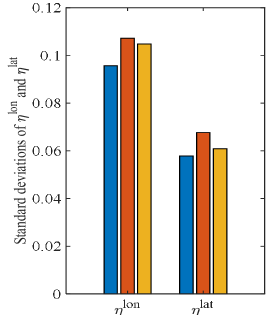
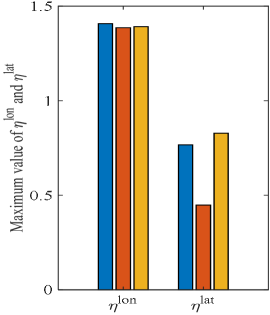
(a)	(b)	(c)
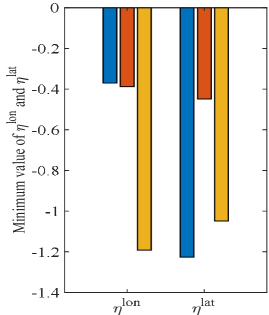
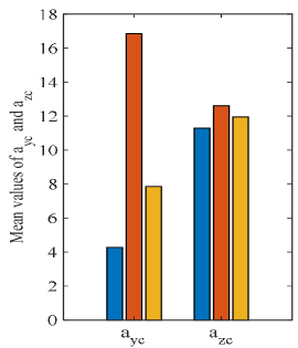
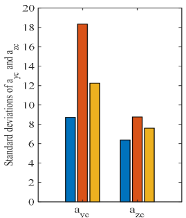
(d)	(e)	(f)

Figure 11: The comparative experiments, conducted for path $\mathcal{P}_{1}$, involve three specific types of RLLP algorithms: RLLP, RLLP with compensation term, and RLLP with optimized compensation term, under different metrics. (a):Comparison of the average values of the time-series data of $\eta^{lon}$ and $\eta^{lat}$; (b) Comparison of the standard deviations of the time-series data of $\eta^{lon}$ and $\eta^{lat}$; (c) Comparison of the maximum values of the time-series data of $\eta^{lon}$ and $\eta^{lat}$; (d) Comparison of the minimum values of the time-series data of $\eta^{lon}$ and $\eta^{lat}$; (e) Comparison of the average values of the time-series data of $a_{yc}$ and $a_{zc}$; (f) Comparison of the standard deviations of the time-series data of $a_{yc}$ and $a_{zc}$.

V-C Optimal Compensation Effect under Large Disturbance

To further analyze the finite-time stabilization performance of the Optimal RLLP guidance law on position error and angular error under large-disturbance condition, we conduct a path-following experiment with noise disturbance at a considerable magnitude of $L_{d}=\frac{\pi}{4}$. Specifically, we use the distance error $e_{d}$ to measure the distance between the current location point $(x_{p},y_{p},z_{p})$ of the fixed-wing UAV and the virtual target point $(x_{g},y_{g},z_{g})$ to be pursued, as follows

$$e_{d}=\sqrt{(x_{p}-x_{g})^{2}+(y_{p}-y_{g})^{2}+(z_{p}-z_{g})^{2}}$$ (46)

As illustrated in Fig.12, even when the UAV encounters large disturbances, leading to a relatively significant fluctuation in its actual flight trajectory, the Optimal RLLP guidance law remains effective. It can drive the distance error $e_{d}$ between the UAV and the virtual target point to converge almost linearly and be stabilized to zero within an average time of less than 10 seconds. Despite the potential risk that an inappropriate selection of the reference point may cause an exceedingly large peak in the distance error, such misselection is promptly corrected during the UAV’s flight. Furthermore, as depicted in Fig.13 and Fig.14, under the circumstances of both constrained input acceleration commands and large-scale disturbances, the Optimal RLLP guidance law is capable of enabling the UAV to follow the reference paths along the $x$, $y$, and $z$-axes with better performance to the fullest extent. Additionally, during each instance of following the virtual target point, $\eta^{lon}$ and $\eta^{lat}$ still demonstrate a rapid convergence trend within a finite time.

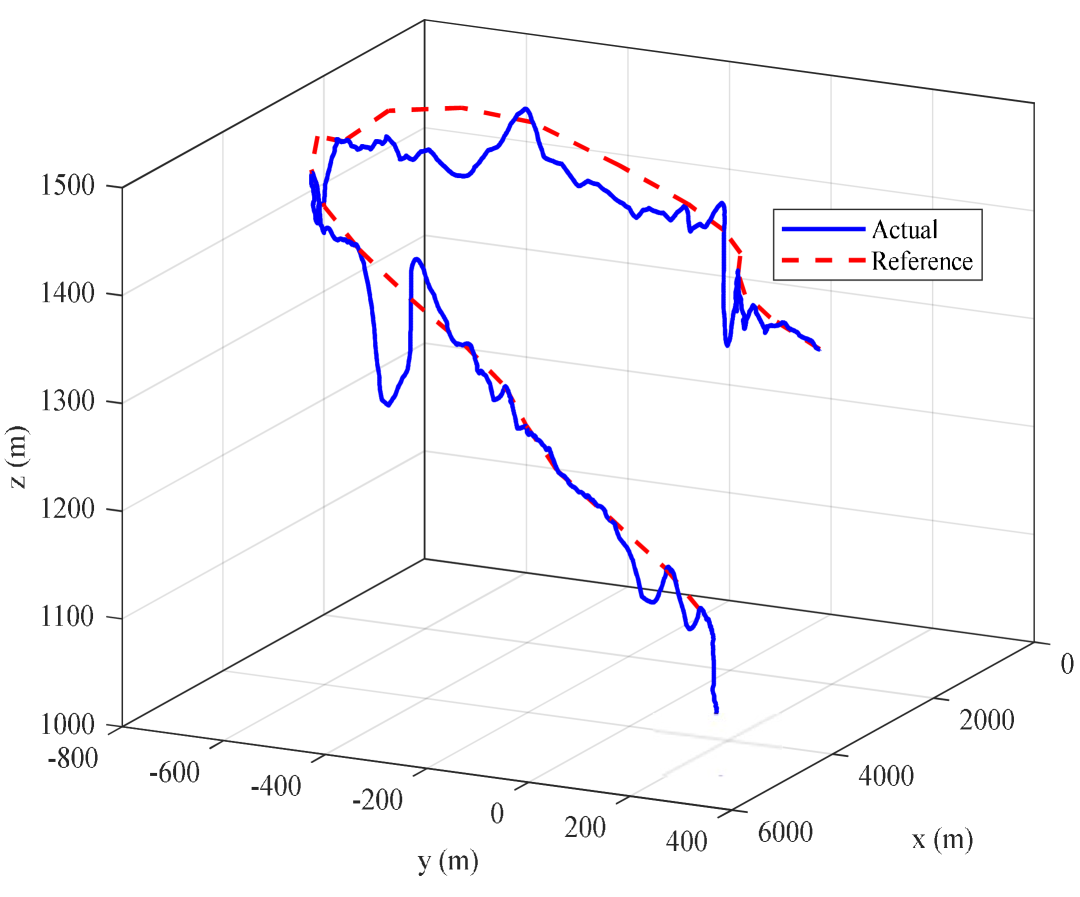
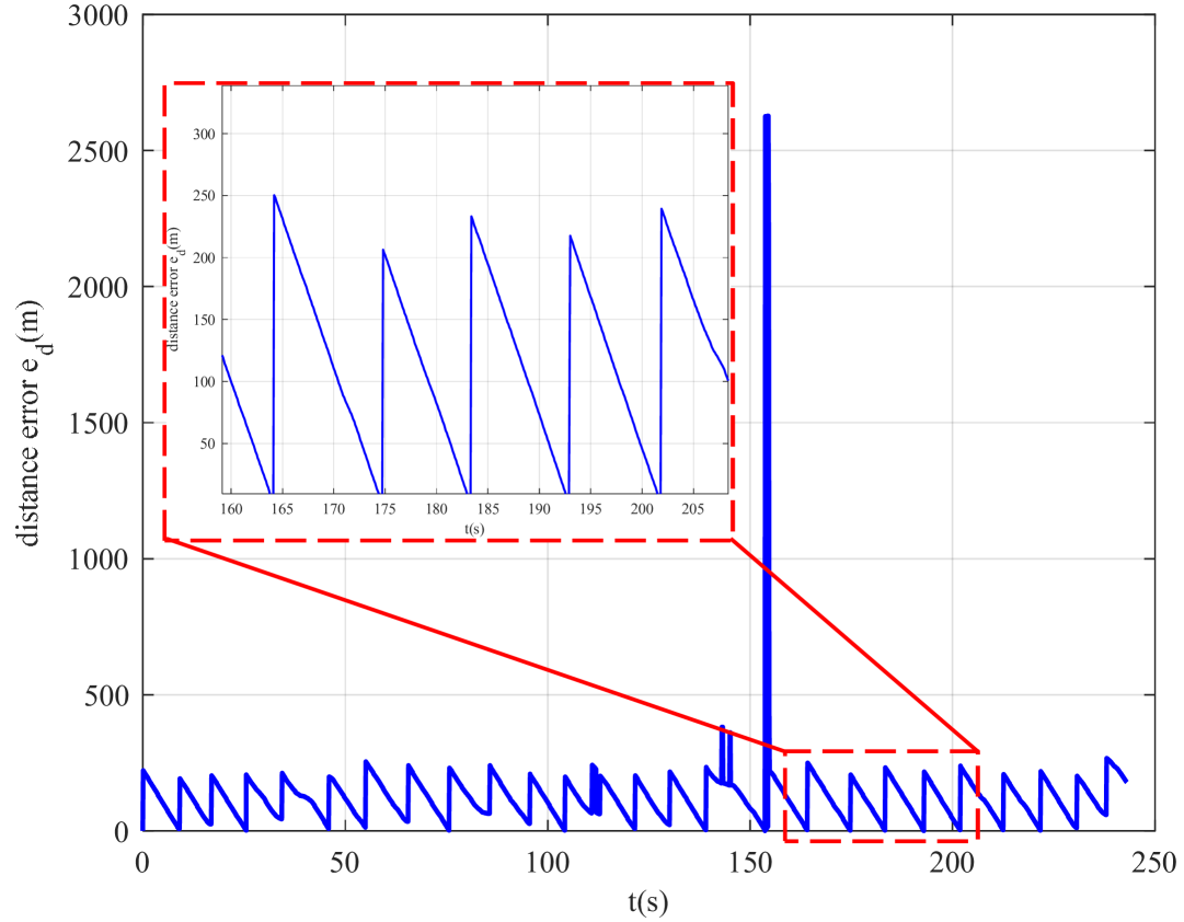
(a)	(b)

Figure 12: The path following performance of the optimal RLLP guidance law under the large disturbance $L_{d}=\frac{\pi}{4}$ on $\mathcal{P}_{1}$ and the time-series curve of the distance error $e_{d}$. (a): The performance of optimal RLLP under $L_{d}=\frac{\pi}{4}$; (b): Sequence data of the distance error $e_{d}$.

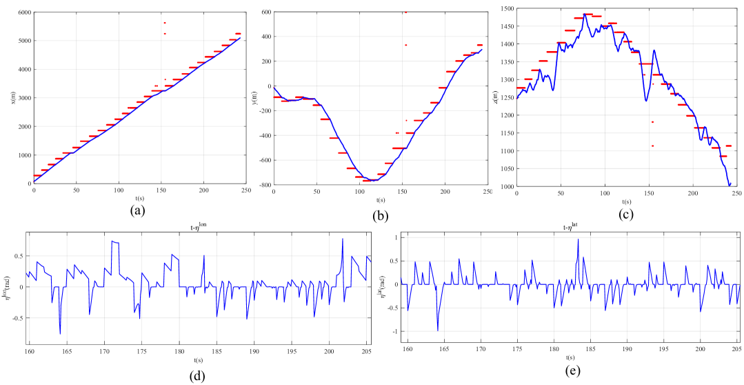
Figure 13: The reference tracking curves along the $x,y$ and $z$-axes, as well as the convergence curves of $\eta^{lon}$ and $\eta^{lat}$ under large-disturbance condition $L_{d}=\frac{\pi}{4}$ when path $\mathcal{P}_{1}$ is followed. (a):Reference tracking curve along the $x$-axe; (b):Reference tracking curve along the $y$-axe; (c):Reference tracking curve along the $z$-axe; (d):The convergence curves of $\eta^{lon}$; (e):The convergence curves of $\eta^{lat}$.

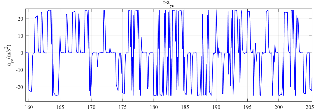
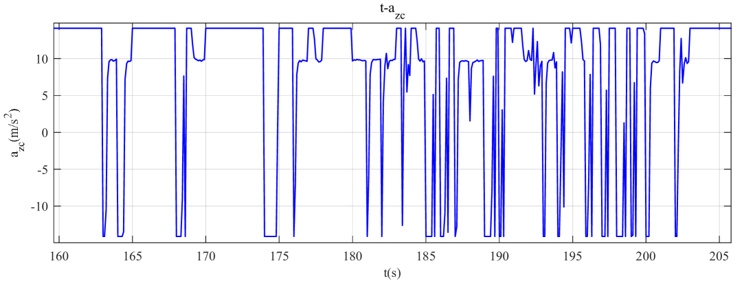
(a)	(b)

Figure 14: Acceleration input commands $a_{yc},a_{zc}$ when path $\mathcal{P}_{1}$ is followed under large disturbance. (a): $a_{yc}$; (b): $a_{zc}$.

VI Conclusion

In an effort to solve the problem of achieving robust and efficient path following for fixed-wing UAVs in low-altitude airspace under externally constrained disturbances, we put forward the Robust Longitudinal-Lateral Look -ahead Pursuit (RLLP) path-following guidance law. By adding specific compensation terms, we have successfully realized the finite-time stabilization of the look-ahead angles and path-following errors. To further mitigate the oscillations of errors and input commands during the operation, we optimized the RLLP guidance law from the aspect of minimizing input energy consumption. Experimental results demonstrate that the optimized RLLP is capable of ensuring the smoothness of sequential input commands while maintaining robustness and finite-time stability.

For future research, the focus should be on devising a more rational form of compensation terms. This is crucial for ensuring the optimal minimization of error oscillations and the shortening of the convergence time of path-following errors under the condition of finite-time stabilization. Additionally, the effective stabilization when the first-order and second-order differentials of input control commands are subject to constraints should also be incorporated into the scope of subsequent research considerations.

Sheng Zimao is born in September, 1999, in Xiaogan, Hubei, PR.China. He is currently working toward the Ph.D. degree in the school of mechanical engineering, Northwestern Polytechnical University, Xi’an Shaanxi, P.R.China. He held the bachelor’s degree of mechanical engineering in Qinghai University, Qinghai, P.R.China in 2021. His current research interests focus on UAV flight motion planning, guidance law, adaptive robust control, active disturbance rejection control, model predictive control, distributed task allocation.

Hong’an Yang received his Ph.D. degree in mechatronic engineering from Northwestern Polytechnical University, Xi’an, China in 2004. He is now a professor in school of Mechanical Engineering, Northwestern Polytechnical University. His major research interests are in the areas of UAV flight planning and control, multi-robot systems, robotic manipulation of deformable objects and intelligent scheduling optimization.

ZiRui Yu is born in February 2003 in Xiaogan, Hubei, China, he is currently pursuing his bachelor’s degree at Tianjin University of Science and Technology in Tianjin, China. His current research interests focus on computer vision, artificial intelligence, and object detection.

Jiakang Wang Jiakang Wang obtained his B.S. degree in mechanical design manufacture and automation from Beijing University of Chemical Technology, Beijing, China in 2017. He received M.S. degree in mechanical engineering from the Beijing University of Chemical Technology, Beijing, China in 2020. He is currently a Ph.D. student at the school of Mechanical Engineering in Northwestern Polytechnical University, Xi’an, China, where he is focusing his research on deformable objects manipulation by robot.

References

- [1] A Pedro Aguiar and Joao P Hespanha. Trajectory-tracking and path-following of underactuated autonomous vehicles with parametric modeling uncertainty. IEEE transactions on automatic control, 52(8):1362–1379, 2007.
- [2] A Pedro Aguiar, Joao P Hespanha, and Petar V Kokotović. Performance limitations in reference tracking and path following for nonlinear systems. Automatica, 44(3):598–610, 2008.
- [3] PB Sujit, Srikanth Saripalli, and Joao Borges Sousa. Unmanned aerial vehicle path following: A survey and analysis of algorithms for fixed-wing unmanned aerial vehicless. IEEE Control Systems Magazine, 34(1):42–59, 2014.
- [4] Saurabh Kumar, Shashi Ranjan Kumar, and Abhinav Sinha. Robust path-following guidance for an unmanned vehicle. In AIAA SCITECH 2023 Forum, page 1055, 2023.
- [5] Praveen Kumar Ranjan, Abhinav Sinha, and Yongcan Cao. Robust uav guidance law for safe target circumnavigation with limited information and autopilot lag considerations. In AIAA SCITECH 2024 Forum, page 0124, 2024.
- [6] Saurabh Kumar, Shashi Ranjan Kumar, and Abhinav Sinha. Three-dimensional path-following nonlinear guidance for unmanned aerial vehicles. Journal of Guidance, Control, and Dynamics, 47(6):1231–1240, 2024.
- [7] Isaac Kaminer, António Pascoal, Enric Xargay, Naira Hovakimyan, Chengyu Cao, and Vladimir Dobrokhodov. Path following for small unmanned aerial vehicles using l1 adaptive augmentation of commercial autopilots. Journal of guidance, control, and dynamics, 33(2):550–564, 2010.
- [8] Patrick Piprek, Haichao Hong, and Florian Holzapfel. Optimal trajectory design accounting for robust stability of path-following controller. Journal of Guidance, Control, and Dynamics, 45(8):1385–1398, 2022.
- [9] Takeshi Yamasaki, SN Balakrishnan, and Hiroyuki Takano. Separate-channel integrated guidance and autopilot for automatic path-following. Journal of Guidance, Control, and Dynamics, 36(1):25–34, 2013.
- [10] Ahmed S Rezk, Horacio M Calderón, Herbert Werner, Benjamin Herrmann, and Frank Thielecke. Predictive path following control for fixed wing uavs using the qlmpc framework in the presence of wind disturbances. In AIAA SCITECH 2024 Forum, page 1594, 2024.
- [11] Jun Yang, Cunjia Liu, Matthew Coombes, Yunda Yan, and Wen-Hua Chen. Optimal path following for small fixed-wing uavs under wind disturbances. IEEE Transactions on Control Systems Technology, 29(3):996–1008, 2020.
- [12] Weijia Yao, Héctor Garcia de Marina, Bohuan Lin, and Ming Cao. Singularity-free guiding vector field for robot navigation. IEEE Transactions on Robotics, 37(4):1206–1221, 2021.
- [13] Weijia Yao. Path following control in 3d using a vector field. In Guiding Vector Fields for Robot Motion Control, pages 39–62. Springer, 2023.
- [14] Zian Wang, Zheng Gong, Jinfa Xu, Jin Wu, and Ming Liu. Path following for unmanned combat aerial vehicles using three-dimensional nonlinear guidance. IEEE-ASME TRANSACTIONS ON MECHATRONICS, 27(5):2646–2656, OCT 2022.
- [15] Saurabh Kumar, Abhinav Sinha, and Shashi Ranjan Kumar. Robust path-following guidance for an autonomous vehicle in the presence of wind. AEROSPACE SCIENCE AND TECHNOLOGY, 150, JUL 2024.
- [16] Randal W Beard, Jeff Ferrin, and Jeffrey Humpherys. Fixed wing uav path following in wind with input constraints. IEEE Transactions on Control Systems Technology, 22(6):2103–2117, 2014.
- [17] Thomas Stastny. L1 guidance logic extension for small uavs: handling high winds and small loiter radii. arXiv preprint arXiv:1804.04209, 2018.
- [18] Cunjia Liu, Owen McAree, and Wen-Hua Chen. Path-following control for small fixed-wing unmanned aerial vehicles under wind disturbances. International Journal of Robust and Nonlinear Control, 23(15):1682–1698, 2013.
- [19] Toufik Souanef. adaptive path-following of small fixed-wing unmanned aerial vehicles in wind. IEEE Transactions on Aerospace and Electronic Systems, 58(4):3708–3716, 2022.
- [20] Weinan Wu, Yao Wang, Chunlin Gong, and Dan Ma. Path following control for miniature fixed-wing unmanned aerial vehicles under uncertainties and disturbances: a two-layered framework. NONLINEAR DYNAMICS, 108(4):3761–3781, JUN 2022.
- [21] Isaac Kaminer, Antonio Pascoal, Enric Xargay, Naira Hovakimyan, Chengyu Cao, and Vladimir Dobrokhodov. Path following for unmanned aerial vehicles using adaptive augmentation of commercial autopilots. JOURNAL OF GUIDANCE CONTROL AND DYNAMICS, 33(2):550–564, MAR-APR 2010.
- [22] Taro YoszAwA. Stability of sets and perturbed system. Funkcialaj Ekvacioj, 5:31–69, 1962.