Micro-canonical cascades and random homeomorphisms

Abstract.

We obtain the Fourier dimension formula for the Mandelbrot micro-canonical cascade measure. Combining with our previous work on the canonical cascade measure, we complete the Mandelbrot-Kahane problem of the Fourier decay of Mandelbrot’s turbulence cascade measures. In addition, we get a two-sided Frostman regularity estimate of the microcanonical cascade measure. As a corollary, we show that almost surely the Dubins-Freedman random homeomorphism is bi-Hölder continuous with “almost” sharp exponents.

1. Introduction

Influenced by the turbluence theory of Kolmogorov-Obukhov-Yaglom, Mandelbrot introduce multiplicative cascade turbluence models. Mandelbrot’s theory is to construct and analyze random fractal measures on the unit interval $[0,1]$ which are generated by two forms: the microcanonical (or conservative) and canonical ones [20, page 67].

In the 1970s, wih the development of fractial analysis, Mandelbrot recognized that it was the time to explore the multifractal properties of cascade measures. He proposed several specific conjectures and fundamental questions, including non-degeneracy, the existence of finite moments, and the Hausdorff dimension of the canonical cascade measure.

Mandelbrot’s conjectures were soon validated by Kahane and Peyrière in [12]. Their results were subsequently generalized by Holley and Waymire [10], Ben Nasr [2], and Waymire and Williams [24], which includ the multifractal properties of microcanonical cascade measure as particular examples(see [7, Corollary 2.1]).

In the 1970s, Mandelbrot also recognized the roles of harmonic analysis on multiplicative cascade models. He hoped that the understanding of multiplicative cascades may at long last benefit from results in harmonic analysis. In particular, he asked the question of the optimal Fourier decay of cascade measures. In 1993, Kahane [11] reanalyzed Mandelbrot’s problem and presented a detailed program for studying the Fourier decay of natural random measures. The Fourier decay of cascade measures is then known as the Mandelbrot-Kahane problem.

By introducing vector-valued martingale theory to the canonical casacde theory, in our recent work [4], announced in [5], we provide a solution to the Mandelbrot-Kahane problem for the canonical case and derive the precise Fourier dimension formula for the Mandelbrot canonical cascade measure.

The goal of current paper is to present a solution to the Mandelbrot-Kahane problem for the microcanonical cascade measure.

Recall that Mandelbrot’s microcanonical cascade measure [18] is constructed by a random vector $W=(W_{0},W_{1})$ with positive coordinates ($W_{0}>0$ and $W_{1}>0\,\,a.s.$) such that

(1.1) $$W_{0}+W_{1}=1\,\,a.s.\text{\, and \,}\mathbb{E}[W_{0}]=\mathbb{E}[W_{1}]=1/2.$$

The microcanonical cascade model also naturally includes the random homeomorphism on $[0,1]$ constructed by Dubins and Freedman in [6] (see [25, Page 305]). As noted by Graf, Mauldin, and Williams in [8], the Dubins-Freedman random homeomorphism and its quantitative properties are closed to an old question posed by S. Ulam. Moreover, the Dubins-Freedman random homeomorphism is the key step for Kozma and Olevskiĭ’s solutions to Luzin problem on the convergence properties of Fourier series by change of variable and related questions [16, 15, 17].

By using wavelet analysis, Resnick-Samorodnitsky-Gilbert-Willinger further studied the microcanonical cascades measures in [22]. Their work goes beyond the classical turbulence cascade models, which is also motivated by Internet WAN traffic studied by Feldmann-Gilbert -Willinge in [1]. Moreover, multiplicative microcanonical cascades has many applications in stock prices [19], river flow and rainfall [9].

Throughout the following, we assume that $W_{0}$ is not identically $1/2$. We will consider the random vector $W=(W_{0},W_{1})$ that satisfies the condition (1.1). We note that the random variables in the work of Resnick-Samorodnitsky-Gilbert-Willinger satisfy the condition (1.1). Moreover, recall that, in Dubins-Freedman’s orignial construction as well as the one studied by Graf-Mauldin-Williams and Kozma-Olevskiĭ, the related random vector is

(1.2) $$W\stackrel{{\scriptstyle d}}{{=}}(U,1-U)\quad\text{with $U$ being uniformly distributed on $(0,1)$}.$$

Let $\mu_{\infty}$ be the Mandelbrot microcanonical cascade measure. Denote its Fourier transform by

$$\widehat{\mu}_{\infty}(\zeta)=\int_{[0,1]}e^{2\pi it\zeta}d\mu_{\infty}(t),\quad\zeta\in\mathbb{R}.$$

The Fourier dimension of $\mu_{\infty}$ is defined by

$$\dim_{F}(\mu_{\infty}):=\sup\{D\in[0,1]:|\widehat{\mu}_{\infty}(\zeta)|^{2}=O(|\zeta|^{-D})\}.$$

Set

(1.3) $$D_{F}=D_{F}(W):=\log_{2}\Big{(}\frac{1}{\mathbb{E}[W_{0}^{2}]+\mathbb{E}[W_{1}^{2}]}\Big{)}=\log_{2}\Big{(}\frac{1}{2\mathbb{E}[W_{0}^{2}]}\Big{)}.$$

Observe that $\mathbb{E}[W_{0}^{2}]=\mathbb{E}[W_{1}^{2}]\in(1/4,1/2)$, then $D_{F}\in(0,1)$.

Theorem 1.1 (Fourier dimension).

Almost surely, we have $\mathrm{dim}_{F}(\mu_{\infty})=D_{F}.$

We also have learned from [22] that the distribution of the generating random vectors can be inferred from the local behavior of signals or samples of the microcanonical cascades. This behavior can be mathematically expressed in terms of the local Hölder exponents of the signal or sample. The Hölder property is, in turn, determined by the Frostman regularity of the cascade measure (see Theorem 1.2 and Corollary 1.3 below). Meanwhile, by Graf-Mauldin-Williams[8] and Kozma-Olevskiĭ[15], almost surely the Dubins-Freedman random homeomorphism is Hölder continuous.

Define

(1.4) $$\gamma_{o}^{+}=\gamma_{o}^{+}(W):=\sup_{p>0}\frac{\log_{2}\big{[}(\mathbb{E}[W_{0}^{p}]+\mathbb{E}[W_{1}^{p}])^{-1}\big{]}}{p};$$

(1.5) $$\gamma_{o}^{-}=\gamma_{o}^{-}(W):=\inf_{p>0}\frac{\log_{2}\big{[}\mathbb{E}[W_{0}^{-p}]+\mathbb{E}[W_{1}^{-p}]\big{]}}{p}.$$

Theorem 1.2 (Frostman regularity).

Almost surely, for any $\varepsilon>0$, there exist $C_{\varepsilon}>1$, such that for any sub-interval $I\subset[0,1]$,

(1.6) $$\frac{1}{C_{\varepsilon}}|I|^{\gamma_{o}^{-}+\varepsilon}\leq\mu_{\infty}(I)\leq C_{\varepsilon}|I|^{\gamma_{o}^{+}-\varepsilon}.$$

If $\gamma_{o}^{-}=+\infty$, then we shall understand the left-hand side of (1.6) as $|I|^{+\infty}=0$ for $|I|<1$.

Remark.

By Lemmas 7.1 and 7.2 below, we know that $\gamma_{o}^{+}\in(0,1)$ and $\gamma_{o}^{-}\in(1,\infty]$.

Remark.

It is worthwhile to mention that, in general, the upper Frostman regularity can not guarantee the positive Fourier dimension of a measure. For instance, the classical Cantor-Lebesgue measure $\mu_{\mathrm{CL}}$ on the one-third Cantor subset of $[0,1]$ is upper Frostman regular with an exponent $\frac{\log 2}{\log 3}$, but the Fourier coefficients of $\mu_{\mathrm{CL}}$ has no Fourier decay since $\widehat{\mu_{\mathrm{CL}}}(3n)=\widehat{\mu_{\mathrm{CL}}}(n)$ for any $n\in\mathbb{N}$. That is, $\dim_{F}(\mu_{\mathrm{CL}})=0$.

Given a microcanonical cascade measure $\mu_{\infty}$ with a random vector $W=(W_{0},W_{1})$, the corresponding random homeomorphism $F_{\infty}$ of the unit interval (called Dubins-Freedman random homeomorphism, see §2.2 for more details) is defined by

$$F_{\infty}(t)=\mu_{\infty}([0,t]),\quad t\in[0,1].$$

Corollary 1.3.

Almost surely, the Dubins-Freedman random homeomorphism $F_{\infty}$ is Hölder continuous of order $\gamma_{o}^{+}-\varepsilon$ for any $\varepsilon>0$ and the inverse Dubins-Freedman random homeomorphism $F_{\infty}^{-1}$ is Hölder continuous of order $(\gamma_{o}^{-})^{-1}-\varepsilon$ for any $\varepsilon>0$.

Remark.

Kozma and Olevskiĭ [15, Remarks after Lemma 1.4] already obtained (1.6) in the case when the random vector $W$ is given by

$$W\stackrel{{\scriptstyle d}}{{=}}(U,1-U)\quad\text{with $U$ being uniformly distributed on $(0,1)$}.$$

We highly believe that the formalism developed by Kozma and Olevskiĭ could be extended beyong the case (1.2). However, even in the case of (1.2), our proof strategies differ significantly from theirs.

Remark.

In the sequel to this paper, we shall show that, under a mild additional assumption on the random vector $W$ (in particular, the random vector $W$ given in (1.2) satisfies our assumption), the two-sided inequalities (1.6) can be improved to be

$$c|I|^{\gamma_{o}^{-}}\leq\mu_{\infty}(I)\leq C|I|^{\gamma_{o}^{+}}$$

and $\gamma_{o}^{\pm}$ are both sharp in the sense that, for any $\delta>0$,

$$\sup_{I}\frac{\mu_{\infty}(I)}{|I|^{\gamma_{o}^{+}+\delta}}=\infty\text{\, and \,}\inf_{I}\frac{\mu_{\infty}(I)}{|I|^{\gamma_{o}^{-}-\delta}}=0\quad a.s.$$

1.1. Outline of the proof of Theorem 1.1

One of the key ingredient is the estimate of the following Sobolev-type norm on $\mu_{\infty}$.

Step 1. Polynomial Fourier decay via vector-valued martingale estimates.

Proposition 1.4.

For any $\varepsilon>0$, there exists $q>2$ large enough such that

$$\mathbb{E}\Big{[}\Big{\{}\sum_{n\in\mathbb{Z}}\big{(}|n|^{\frac{D_{F}}{2}-\varepsilon}\cdot|\widehat{\mu}_{\infty}(n)|\big{)}^{q}\Big{\}}^{2/q}\Big{]}<\infty.$$

Step 2. Optimality of the polynomial exponent: fluctuation of branching random walks.

Consider

$$\mathcal{M}_{n}^{(2)}=\frac{1}{2^{n}}\sum_{|u|=n}\prod_{j=1}^{n}\frac{W_{u_{j}}(u|_{j-1})^{2}}{\mathbb{E}[W_{0}^{2}]},\quad n\geq 1.$$

It can be checked that $(\mathcal{M}_{n}^{(2)}:n\geq 1)$ is a positive martingale and hence converges to a limit denoted by $\mathcal{M}_{\infty}^{(2)}$. In Lemma 5.6 below, we shall prove that $\mathbb{P}(\mathcal{M}_{\infty}^{(2)}>0)=1$.

Denote by

$$\varrho=\mathbb{E}[|\widehat{\mu}_{\infty}(1)|^{2}]\quad\text{\, and \,}\quad\varpi=\mathbb{E}[\widehat{\mu}_{\infty}(1)^{2}].$$

In Lemma 5.2 below, we shall show that $\varphi$ is a real number. Indeed, we show that $\varpi<0$ and $\varrho\pm\varpi>0$.

Proposition 1.5.

Along the dyadic subsequence, the fluctuation of the rescaled Fourier coefficients $\widehat{\mu}_{\infty}(2^{n})$ is given by

$$2^{\frac{nD_{F}}{2}}\widehat{\mu}_{\infty}(2^{n})\xrightarrow[n\to\infty]{d}\sqrt{\mathcal{M}_{\infty}^{(2)}}\cdot\mathcal{N}_{\mathbb{C}}(0,\Sigma),$$

where $\mathcal{N}_{\mathbb{C}}(0,\Sigma)$ is the complex random Gaussian with covariance matrix given by

$$\Sigma=\frac{1}{2}\begin{pmatrix}\varrho+\varpi&0\\ 0&\varrho-\varpi\\ \end{pmatrix}.$$

Moreover $\mathcal{N}_{\mathbb{C}}(0,\Sigma)$ and $\mathcal{M}_{\infty}^{(2)}$ are independent.

Step 3. The almost sure equality $\dim_{F}(\mu_{\infty})=D_{F}$.

Proposition 1.4 implies the almost sure inequality $\dim_{F}(\mu_{\infty})\geq D_{F}$ and Proposition 1.5 implies the almost sure converse inequality $\dim_{F}(\mu_{\infty})\leq D_{F}.$ See §6 for the details.

Acknowledgements.

This work is supported by the NSFC (No.12288201). XC is supported by Nation Key R&D Program of China 2022YFA1006500. YH is supported by NSFC 12131016 and 12201419, ZW is supported by NSF of China 12471116.

2. Preliminaries

2.1. Mandelbrot’s microcanonical cascade

Recall that the standard dyadic symtem on the $[0,1]$ can naturally be identified with the rooted binary tree $\mathcal{T}_{2}$ (with the root denoted by $\emptyset$) with

$$\mathcal{T}_{2}=\{\emptyset\}\sqcup\bigsqcup_{n\geq 1}\{0,1\}^{n}.$$

For any $u\in\mathcal{T}_{2}$, it can be written as $u=x_{1}x_{2}\cdots x_{n}$ with $x_{j}\in\{0,1\}$ and induces a dyadic interval $I_{u}\subset[0,1)$ as

$$I_{u}=\Big{[}\sum_{1}^{|u|}u_{k}2^{-k},\sum_{1}^{|u|}u_{k}2^{-k}+2^{-n}\Big{)}\text{\, and \,}I_{\emptyset}=[0,1).$$

We set $|u|=n,u_{j}=x_{j}$ and $u|_{k}=x_{1}\cdots x_{k}$ (with $u|_{0}=\emptyset$).

Given any random vector $W=(W_{0},W_{1})$ with

$$0<W_{0}<1\text{\, and \,}W_{0}+W_{1}=1\,\,a.s.$$

For any $n\geq 1$, the random probability measure $\mu_{n}$ defined in (2.5) is given by

(2.1) $$\mu_{n}(dt)=\sum_{|u|=n}\prod_{j=1}^{n}X(u|_{j})\cdot\mathds{1}_{I_{u}}(t)dt,$$

where $(X(u))_{u\in\mathcal{T}_{2}\setminus\{\emptyset\}}$ is the stochastic process on $\mathcal{T}_{2}\setminus\{\emptyset\}$ with $\mathbb{E}[X(u)]=1$ and defined as follows (see Figure 1 for an illustration): if $u=u_{1}\cdots u_{n}\in\{0,1\}^{n}$, then

(2.2) $$X(u):=2W_{u_{n}}(u_{1}\cdots u_{n-1}).$$

In particular, the random variable $X(u|_{j})$ is given by

$$X(u|_{j})=2W_{u_{j}}(u|_{j-1}).$$

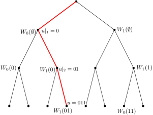
Figure 1. An illustration of the stochastic process $(\frac{X(u)}{2})_{u\in\mathcal{T}_{2}\setminus\{\emptyset\}}$

By Kahane’s fundamental theory of $T$-martingales, almost surely, the random probability measures $\mu_{n}$ converge weakly to a limit random probability measure, denoted by $\mu_{\infty}$:

(2.3) $$\mu_{n}\xrightarrow[n\to\infty]{\text{weakly}}\mu_{\infty},\quad a.s.$$

The limit random measure $\mu_{\infty}$ is called the Mandelbrot’s microcanonical cascade measure (also called the micro-canonical cascades [20, p. 311, §3.4]).

It is knwon that $\mu_{\infty}([0,1])=1$ almost surely and $\mu_{\infty}$ is supported on a Borel set of Hausdorff dimension $-2\mathbb{E}[W\log_{2}W]$.

2.2. Dubins-Freedman random homeomorphisms

In the following, we briefly recall the constructions of Dubins and Freedman, as well as Graf, Mauldin, and Williams [8], on random homeomorphisms of $[0,1]$.

Let $(W(u))_{u\in\mathcal{T}_{2}}$ be the i.i.d. copies of two dimensionanl random vector $W=(W_{0},W_{1})$ with satisfying the condition (1.1).. For each random vector $W(u)$, write

$$W(u)=(W_{0}(u),W_{1}(u)).$$

For each integer $n\geq 1$, define a random step function $\rho_{n}$ by

$$\rho_{n}(t):=\sum_{|u|=n}2W_{u_{n}}(u_{1}\cdots u_{n-1})\cdot\mathds{1}_{I_{u}}(t).$$

Then, consider the random homeomorphism $F_{n}$ between $[0,1]$ by

(2.4) $$F_{n}(t)=\int_{0}^{t}f_{n}(s)ds\quad\text{with\,}f_{n}(t):=\prod_{j=1}^{n}\rho_{j}(t).$$

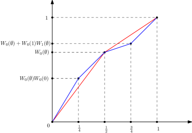
Figure 2. The first two constructions $F_{1}$ (the red one) and $F_{2}$ (the blue one)

Follows from the main result in [8, Theorem 2.6], almost surely, $F_{n}$ converges uniformly to a random homeomorphism $F_{\infty}$ of $[0,1)$ (which clearly has a natural extension to a homeomorphism of the closed unit interval).

2.3. Connections

The study of the random homeomorphisms $F_{n}$ and $F_{\infty}$ can be naturally put into the context of microcanonical Mandelbrot cascades. Here we briefly explain the connection. Indeed, we denote the random probability measure $dF_{n}$ by

(2.5) $$\mu_{n}(dt)=dF_{n}(t)=\prod_{j=1}^{n}\rho_{j}(t)dt\,\,\text{for $n\geq 1$}.$$

By convention, we set $\mu_{0}(dt)=dt$. Since $(\rho_{n}(t))_{n\geq 1}$ are independent random functions and $\mathbb{E}[\rho_{n}(t)]\equiv 1$, one easily sees that the sequence $(f_{n}(t))_{n\geq 1}$ forms a natural non-negative $T$-martingale in the sense of Kahane [13, 14], with respect to the natural filtration:

(2.6) $$\mathscr{F}_{n}=\sigma\Big{(}\Big{\{}\rho_{k}(t):k\leq n\Big{\}}\Big{)}=\sigma\Big{(}\Big{\{}W(u):|u|\leq n-1\Big{\}}\Big{)}\,\,\text{for $n\geq 1$},$$

where we used the fact that the definition of the random function $\rho_{k}$ involves only the random vectors

$$W(u_{1}\cdots u_{k-1})=(W_{0}(u_{1}\cdots u_{k-1}),W_{1}(u_{1}\cdots u_{k-1}))\,\,\text{for all $u_{1}\cdots u_{k-1}\in\{0,1\}^{k-1}$. }$$

By convention, we set $\mathscr{F}_{0}$ to be the trivial sigma-algebra.

Due to the self-similarity structure, the sequence $(\mu_{n})_{n\geq 1}$ and the limit random probability measure $\mu_{\infty}$ can be put into the context of To see the equality (2.1), it suffices to notice that, for any $n\geq 1$ and any $u=u_{1}\cdots u_{n}\in\{0,1\}^{n}$, we have

(2.7) $$\frac{d\mu_{n}}{dt}\Big{|}_{I_{u}}=\prod_{j=1}^{n}\rho_{j}(t)\Big{|}_{I_{u}}=2^{n}\cdot W_{u_{1}}(\emptyset)W_{u_{2}}(u_{1})W_{u_{3}}(u_{1}u_{2})\cdots W_{u_{n}}(u_{1}u_{2}\cdots u_{n-1}).$$

2.4. Notation

Throughout the paper, by writing $A\lesssim_{x,y}B$, we mean there exists a finite constant $C_{x,y}>0$ depending only on $x,y$ such that $A\leq C_{x,y}B$. And, by writing $A\asymp_{x,y}B$, we mean $A\lesssim_{x,y}B$ and $B\lesssim_{x,y}A$.

By convention, for any sequence $(c_{j})_{j\geq 1}$ in $\mathbb{C}$, we write

$$\prod_{j=1}^{0}c_{j}=\prod_{j\in\emptyset}c_{j}=1\text{\, and \,}\sum_{j=1}^{0}c_{j}=\sum_{j\in\emptyset}c_{j}=0.$$

Given any integrable random variable $X$, we shall write $\mathring{X}$ the centerization of $X$:

(2.8) $$\mathring{X}:=X-\mathbb{E}[X].$$

3. A new entropy-type inequality for 2D-random vectors

In this section, we always assume that $V=(V_{0},V_{1})$ is a random vector in $\mathbb{R}_{+}^{2}$ with non-negative coordinates such that

$$V_{0}+V_{1}=1\,\,a.s.$$

And define for any $p>0$,

(3.1) $$K_{V}(p):=\log\big{[}(\mathbb{E}[V_{0}^{p}+V_{1}^{p}])^{1/p}\big{]}=\log\big{[}(\mathbb{E}[\|V\|_{\ell^{p}}^{p}])^{1/p}\big{]}=\log\|V\|_{L^{p}(\ell^{p})},$$

where as usual, for any vector $x\in\mathbb{R}^{d}$ and any $p>0$, we write the $p$-norm

$$\|x\|_{\ell^{p}}=\Big{(}\sum_{i=1}^{d}|x_{i}|^{p}\Big{)}^{1/p}.$$

Note that the $\ell_{p}$-norm of a given vector is non-increasing on $p$ and the $L_{p}$-norm of a given random variable is non-decreasing on $p$. Therefore, a priori, it is not clear whether $K_{V}(p)$ is monotone as a function on $p$.

For $d=2$, we have the following unexpected monotonicity of the function $K_{V}(p)$ on the interval $[1,2]$. The general situation for $d\geq 3$ is not clear at the time of writing.

Proposition 3.1.

The function $K_{V}$ is non-increasing on the interval $[1,2]$. Moreover $K_{V}$ is decreasing on $[1,2]$ provided that $\mathbb{E}[V_{0}V_{1}]>0$. In particular, for all $p\in[1,2]$, the following entropy-type inequality holds

(3.2) $$\mathbb{E}\big{[}V_{0}^{p}\log(V_{0}^{p})+V_{1}^{p}\log(V_{1}^{p})\big{]}\leq\mathbb{E}\big{[}V_{0}^{p}+V_{1}^{p}\big{]}\log\big{(}\mathbb{E}\big{[}V_{0}^{p}+V_{1}^{p}\big{]}\big{)}.$$

Moreover, the equality holds at one point $p\in[1,2]$ if and only if $V_{0}V_{1}=0\,\,a.s.$

Remark 3.1.

By numerical experiments, we know that the inequality (3.2) fails in higher dimension $d\geq 17$. We believe that $17$ is not optimal and it could be that (3.2) already fails for $d=3$. However, at the time of writing, we are not able to prove this.

Lemma 3.2.

We have

(3.3) $$\|V\|_{L^{3}(\ell^{3})}\leq\|V\|_{L^{2}(\ell^{2})},$$

with the equality holds if and only if $V_{0}V_{1}=0\,\,a.s.$

Proof.

By setting

(3.4) $$c=\mathbb{E}[V_{0}]-\mathbb{E}[V_{0}^{2}]=\mathbb{E}[V_{0}V_{1}],$$

we obtain

$$\|V\|_{L^{2}(\ell^{2})}^{2}=\mathbb{E}[V_{0}^{2}]+\mathbb{E}[(1-V_{0})^{2}]=1-2\mathbb{E}[V_{0}]+2\mathbb{E}[V_{0}^{2}]=1-2c$$

and

$$\|V\|_{L^{3}(\ell^{3})}^{3}=\mathbb{E}[V_{0}^{3}]+\mathbb{E}[(1-V_{0})^{3}]=1-3\mathbb{E}[V_{0}]+3\mathbb{E}[V_{0}^{2}]=1-3c.$$

Consequently,

$$\|V\|_{L^{2}(\ell^{2})}^{6}-\|V\|_{L^{3}(\ell^{3})}^{6}=(1-2c)^{3}-(1-3c)^{2}=c^{2}(3-8c).$$

Using the defintion (3.4) for $c$, we have

$$3-8c=3-8\mathbb{E}[V_{0}]+8\mathbb{E}[V_{0}^{2}]=1+8\mathbb{E}[(V_{0}-1/2)^{2}]\geq 1.$$

Then the desired inequality (3.3) follows, with the equality holds if and only if $c=0$, which is equivalent to $V_{0}V_{1}=0\,\,a.s.$ ∎

Proof of Proposition 3.1.

By the standard complex interpolation method on $L^{p}$-spaces (see [3, Chapter 5, Theorem 5.1.1, p.106]), if $\theta\in(0,1)$ and $p_{0},p_{1},p_{\theta}\in[1,\infty)$ satisfy

$$\frac{1}{p_{\theta}}=\frac{1-\theta}{p_{0}}+\frac{\theta}{p_{1}},$$

then

$$\|V\|_{L^{p_{\theta}}(\ell^{p_{\theta}})}\leq\|V\|_{L^{p_{0}}(\ell^{p_{0}})}^{1-\theta}\|V\|_{L^{p_{1}}(\ell^{p_{1}})}^{\theta}.$$

Therefore, by the definition (3.1) of the function $K_{V}$,

$$K_{V}(p_{\theta})\leq(1-\theta)K_{V}(p_{0})+\theta K_{V}(p_{1}).$$

In other words, the function $(0,1]\ni t\mapsto f_{V}(t):=K_{V}(1/t)$ is convex.

Lemma 3.2 implies that $f_{V}(1/3)\leq f_{V}(1/2)$. Hence, by the convexity of $f_{V}$, for any $r,s\in[1,2]$ with $r<s$, then $\frac{1}{r}>\frac{1}{s}>\frac{1}{2}>\frac{1}{3}$ and

$$\frac{K_{V}(r)-K_{V}(s)}{\frac{1}{r}-\frac{1}{s}}=\frac{f_{V}(1/r)-f_{V}(1/s)}{\frac{1}{r}-\frac{1}{s}}\geq\frac{f_{V}(1/2)-f_{V}(1/3)}{\frac{1}{2}-\frac{1}{3}}\geq 0.$$

This implies that $K_{V}$ is non-increasing on the interval $[1,2]$. Lemma 3.2 also implies that if $\mathbb{E}[V_{0}V_{1}]>0$, then $f_{V}(1/2)>f_{V}(1/3)$ and hence $K_{V}$ is decreasing on $[1,2]$. In particular,

$$K_{V}^{\prime}(p)\leq 0\quad\text{for all $p\in[1,2]$},$$

which implies the desired inequality (3.2). Finally, if $\mathbb{E}[V_{0}V_{1}]>0$, then by Lemma 3.2, for any $p\in[1,2]$, we have $1/p\geq 1/2>1/3$ and

$$-p^{2}K_{V}^{\prime}(p)=f_{V}^{\prime}(1/p)\geq\frac{f_{V}(1/2)-f_{V}(1/3)}{\frac{1}{2}-\frac{1}{3}}>0.$$

This completes the whole proof. ∎

4. Polynomial Fourier decay

This section is devoted to the proof of Proposition 1.4. Indeed, it suffices to show that, for any $\varepsilon>0$, there exists a large enough $q>2$ such that

(4.1) $$\mathbb{E}\Big{[}\Big{\{}\sum_{s=1}^{\infty}\big{(}s^{\frac{D_{F}}{2}-\varepsilon}\cdot|\widehat{\mu}_{\infty}(s)|\big{)}^{q}\Big{\}}^{2/q}\Big{]}=\Big{\|}\Big{(}s^{\frac{D_{F}}{2}-\varepsilon}\cdot\widehat{\mu}_{\infty}(s)\Big{)}_{s\geq 1}\Big{\|}_{L^{2}(\ell^{q})}^{2}<\infty.$$

4.1. The $\ell^{q}$-vector valued martingale

Fix any $\alpha$ with

$$0<\alpha<1/2.$$

We are going to study the random vectors in $\mathbb{C}^{\mathbb{N}}$ generated by the Fourier coefficients of the random cascade probability measure $\mu_{\infty}$ obtained in (2.3):

(4.2) $$M=M^{(\alpha)}:=(s^{\alpha}\widehat{\mu}_{\infty}(s))_{s\geq 1}\in\mathbb{C}^{\mathbb{N}}.$$

Alarm:

A priori, we do not know whether, the random vector $M$ in $\mathbb{C}^{\mathbb{N}}$ in (4.2) almost surely represents a vector in $\ell^{q}$.

Definition.

Recall the increasing filtration $(\mathscr{F}_{n})_{n\geq 0}$ of $\sigma$-algebras introduced in (2.6). Recall also the definition of the random measures $\mu_{n}$ given in (2.5) and (2.1). For any integer $n\geq 0$, define a random vector $M_{n}=(M_{n}(s))_{s\geq 1}\in\mathbb{C}^{\mathbb{N}}$ by

(4.3) $$M_{n}(s):=\mathbb{E}[M(s)|\mathscr{F}_{n}]=s^{\alpha}\widehat{\mu}_{n}(s)=s^{\alpha}\int_{[0,1]}e^{2\pi ist}d\mu_{n}(t).$$

Note that $M_{0}(s)\equiv 0$ for all $s\geq 1$.

Now, by Lemma 4.1 below, we can see that $(M_{n})_{n\geq 1}$ is an $\ell^{q}$-vector-valued martingale with $\mathbb{E}[\|M_{n}\|_{\ell^{q}}^{2}]<\infty$. However, the very rough estimate in the proof of Lemma 4.1 does not yield the desired uniform $L^{2}$-boundedness of the martingale $(M_{n})_{n\geq 1}$. Indeed, the uniform $L^{2}$-boundedness of $(M_{n})_{n\geq 1}$ is given in §4.2, where martingale type inequalities will play a key role and will appear in two different places in the proof.

Lemma 4.1 (A very rough estimate).

For any $n\geq 0$ and any $q>\frac{1}{1-\alpha}>2$, we have

$$\mathbb{E}[\|M_{n}\|_{\ell^{q}}^{2}]<\infty.$$

Therefore, $(M_{n})_{n\geq 0}$ is an $\ell^{q}$-vector-valued martingale with respect to the filtration $\mathscr{F}_{n}$.

Proof.

Recall that the random measure $\mu_{n}(dt)=f_{n}(t)dt$ has a random density $f_{n}$ (see (2.4) and (2.7)) and $f_{n}$ is constant on each dyadic interval $I_{u}$ with $|u|=n$. By writing

$$f_{n}(t)|_{I_{u}}:=\underbrace{2^{n}\cdot W_{u_{1}}(\emptyset)W_{u_{2}}(u_{1})W_{u_{3}}(u_{1}u_{2})\cdots W_{u_{n}}(u_{1}u_{2}\cdots u_{n-1})}_{\text{denoted $C_{u}$}},$$

we have, for any integer $s\geq 1$,

$$\widehat{\mu}_{n}(s)=\sum_{|u|=n}\int_{I_{u}}f_{n}(t)e^{2\pi ist}dt=\sum_{|u|=n}C_{u}\int_{I_{u}}e^{2\pi ist}dt.$$

Since $0<W_{u_{k}}(u_{1}\cdots u_{k-1})<1$ for all $|u|=n$ and $k$, we have $0\leq C_{u}\leq 2^{n}$. Hence for any integer $s\geq 1$

$$|\widehat{\mu}_{n}(s)|\leq 2^{n}\sum_{|u|=n}\Big{|}\int_{I_{u}}e^{2\pi ist}dt\Big{|}\leq\frac{4^{n}}{\pi s}.$$

Therefore, by the assumption $q(1-\alpha)>1$ and the following inequality

$$\sum_{s\geq 1}|s^{\alpha}\widehat{\mu}_{n}(s)|^{q}\leq\frac{4^{n}}{\pi^{q}}\sum_{s\geq 1}s^{-(1-\alpha)q},$$

we obtain $\|M_{n}\|_{L^{\infty}(\ell^{q})}<\infty$. The desired inequality follows immediately. ∎

4.2. Uniform $L^{2}$-boundedness of $(M_{n})_{n\geq 0}$ via martingale type inequalities

To prove Proposition 1.4, we need to prove the uniform $L^{2}$-boundedness of the $\ell^{q}$-vector-valued martingale $(M_{n})_{n\geq 0}$ for very large $q$ (see Lemma 4.4 below for the choice of $q$):

(4.4) $$\sup_{n\geq 0}\mathbb{E}[\|M_{n}\|_{\ell^{q}}^{2}]<\infty.$$

The key ingredient in our proof of the inequality (4.4) is twice crucial applications of the martingale type-$2$ inequality of the Banach space $\ell^{q}$ for $q\geq 2$ which is classical in the local theory of Banach spaces (see [21, p. 409, Definition 10.41]): there exists a constant $C_{q}>0$ such that for any $\ell^{q}$-valued martingale $(Z_{m})_{m\geq 0}$ in $L^{2}(\mathbb{P};\ell^{q})$ satisfy

(4.5) $$\mathbb{E}[\|Z_{n}\|_{\ell^{q}}^{2}]\leq C_{q}\sum_{k=0}^{n}\mathbb{E}[\|Z_{k}-Z_{k-1}\|_{\ell^{q}}^{p}]$$

with the convention $Z_{-1}\equiv 0$. In particular, the inequality (4.5) implies in particular that, for any family of independent and centered random variables $(\Delta_{k})_{k=0}^{m}$ in $L^{2}(\mathbb{P};\ell^{q})$,

(4.6) $$\mathbb{E}\Big{[}\Big{\|}\sum_{k=0}^{m}\Delta_{k}\Big{\|}_{\ell^{q}}^{2}\Big{]}\leq C_{q}\sum_{k=0}^{m}\mathbb{E}[\|\Delta_{k}\|_{\ell^{q}}^{2}].$$

The proof of the inequality (4.4) is outlined as follows. In particular, we indicate the two places where the martingale type inequalities are used.

• The first application of martingale type-$2$ inequality: For applying martingale type inequality (4.5) to our $\ell^{q}$ martingale $(M_{n})_{n\geq 0}$ introduced in (4.3), we first define the sequence of the martingale differences $(D_{m})_{m\geq 1}$:

  (4.7) $$D_{m}(s):=M_{m}(s)-M_{m-1}(s)\quad\text{for all $m\geq 1$ and $s\geq 1$}.$$

  Note that, we have $M_{0}\equiv 0$. Hence, by (4.5), we get

  (4.8) $$\mathbb{E}[\|M_{n}\|_{\ell^{q}}^{2}]\leq C_{q}\sum_{m=1}^{n}\mathbb{E}[\|D_{m}\|_{\ell^{q}}^{p}].$$

• The second application of martingale type-$2$ inequality: for each $1\leq m\leq n$, we find that (see Lemma 4.2), each martingale difference $D_{m}$ can be decomposed as the following summation

  $$D_{m}=\sum_{|u|=m-1}\Delta_{u},$$

  where $\Delta_{u}$ are random vectors in $\ell^{q}$ with explicit form (see (4.16) below). From the explicit forms of all the random vectors $\Delta_{u}$, one immediately see that, conditioned on $\mathscr{F}_{m-1}$, they are independent and satisfy $\mathbb{E}[\Delta_{u}|\mathscr{F}_{m-1}]=0$. Consequently, we may apply the conditional version of (4.6) and obtain

  $$\mathbb{E}\big{[}\|D_{m}\|_{\ell^{q}}^{2}\big{|}\mathscr{F}_{m-1}\big{]}\leq C_{q}\sum_{|u|=m-1}\mathbb{E}\big{[}\|\Delta_{u}\|_{\ell^{q}}^{2}\big{|}\mathscr{F}_{m-1}\big{]}.$$

  Therefore, by taking expectation on both sides, we obtain

  (4.9) $$\mathbb{E}\big{[}\|D_{m}\|_{\ell^{q}}^{2}\big{]}\leq C_{q}\sum_{|u|=m-1}\mathbb{E}\big{[}\|\Delta_{u}\|_{\ell^{q}}^{2}\big{]}.$$

• Combining the inequalities (4.8) and (4.9), we obtain

  $$\mathbb{E}[\|M_{n}\|_{\ell^{q}}^{2}]\leq C_{q}^{2}\cdot\sum_{m=1}^{n}\sum_{|u|=m-1}\mathbb{E}\big{[}\|\Delta_{u}\|_{\ell^{q}}^{2}\big{]}.$$

• For each $1\leq m\leq n$ and $|u|=m-1$, it turns out that $\mathbb{E}\big{[}\|\Delta_{u}\|_{\ell^{q}}^{2}\big{]}$ has very simple form and can be effectively upper-estimated.

Now we proceed to the proof of the main inequality (4.4).

We start with introducing some notations. Recall the stochastic process $(X(u))_{u\in\mathcal{T}_{2}\setminus\{\emptyset\}}$ defined in (2.2). Using the notation (2.8), in what follows, we denote

$$\mathring{X}(u)=X(u)-\mathbb{E}[X(u)]=X(u)-1.$$

We shall denote the left end-point of the dyadic interval $I_{u}$ by $\ell_{u}$. That is,

(4.10) $$\ell_{u}:=\sum_{k=1}^{|u|}u_{k}2^{-k}\text{\, and \,}\ell_{\emptyset}=0.$$

It will be convenient for us to denote, for any integers $m,s\geq 1$

(4.11) $$\kappa_{m}(s):=\frac{e^{i2\pi s2^{-m}}-1}{i2\pi s}.$$

And, for any $s,m\geq 1$ and $|u|=m-1$, set

(4.12) $$T(u,s,m):=\mathring{X}(u0)+e^{i2\pi s2^{-m}}\mathring{X}(u1)=2\mathring{W}_{0}(u)+2e^{i2\pi s2^{-m}}\mathring{W}_{1}(u).$$

The martingale differences $D_{m}$ defined in (4.7) has the following explicit form. Recall that, since $M_{0}(s)\equiv 0$ for all $s\geq 1$, by an elementary computation, we have

(4.15) $$D_{1}(s)=M_{1}(s)=\left\{\begin{array}[]{cl}\frac{2i}{\pi}\cdot s^{\alpha-1}\cdot(W_{0}-W_{1})&\text{if $s$ is odd}\\ 0&\text{if $s$ is even}\end{array}\right..$$

Lemma 4.2.

For any $m\geq 2$ and $s\geq 1$, the martingale difference $D_{m}(s)$ is given by

(4.16) $$D_{m}(s)=s^{\alpha}\kappa_{m}(s)\sum_{|u|=m-1}e^{i2\pi s\ell_{u}}\Big{(}\prod_{j=1}^{m-1}X(u|_{j})\Big{)}\cdot T(u,s,m).$$

Proof.

Note that for any $|u|=m$, by the definition (4.11) of $\kappa_{m}(s)$,

(4.17) $$\int_{I_{u}}e^{i2\pi sx}dx=\kappa_{m}(s)e^{i2\pi s\ell_{u}}.$$

By (2.1), for any integer $s\geq 1$,

$$\widehat{\mu}_{m}(s) =\int_{0}^{1}e^{i2\pi sx}d\mu_{m}(x)=\kappa_{m}(s)\cdot\sum_{|u|=m}e^{i2\pi s\ell_{u}}\prod_{j=1}^{m}X(u|_{j}).$$

Thus, by using the equality

$$\frac{\kappa_{m-1}(s)}{\kappa_{m}(s)}=1+e^{i2\pi s2^{-m}},$$

we obtain

$$\widehat{\mu}_{m-1}(s)=\kappa_{m}(s)\cdot\sum_{|v|=m-1}e^{i2\pi s\ell_{v}}\Big{(}\prod_{j=1}^{m-1}X(v|_{j})\Big{)}\cdot(1+e^{i2\pi s2^{-m}}).$$

Now, for each $u$ with $|u|=m$, we may write it as $u=vu_{m}$ with $v=u|_{m-1}$. Then using

$$\ell_{u}=\ell_{v}+u_{m}2^{-m}\text{\, and \,}u|_{j}=v|_{j}\quad\text{for all $j\leq m-1$,}$$

we obtain

$$\widehat{\mu}_{m}(s) =\kappa_{m}(s)\sum_{|v|=m-1}\Big{[}e^{i2\pi s\ell_{v}}\Big{(}\prod_{j=1}^{m-1}X(v|_{j})\Big{)}X(v0)+e^{i2\pi s\ell_{v}}e^{i2\pi s2^{-m}}\Big{(}\prod_{j=1}^{m-1}X(v|_{j})\Big{)}X(v1)\Big{]}$$

$$=\kappa_{m}(s)\sum_{|v|=m-1}e^{i2\pi s\ell_{v}}\Big{(}\prod_{j=1}^{m-1}X(v|_{j})\Big{)}\cdot\Big{(}X(v0)+e^{i2\pi s2^{-m}}X(v1)\Big{)}$$

Consequently, by recalling $\mathring{X}(u)=X(u)-1$, we obtain

$$D_{m}(s)= \widehat{\mu}_{m}(s)-\widehat{\mu}_{m-1}(s)$$

$$= \kappa_{m}(s)\cdot\sum_{|v|=m-1}e^{i2\pi s\ell_{v}}\Big{(}\prod_{j=1}^{m-1}X(v|_{j})\Big{)}\cdot\Big{(}\mathring{X}(v0)+e^{i2\pi s2^{-m}}\mathring{X}(v1)\Big{)}.$$

This completes the proof of the lemma. ∎

Lemma 4.3.

For any $q\geq 2$,

(4.18) $$\mathbb{E}[|T(u,s,m)|^{q}]=2^{q}|1-e^{i2\pi s2^{-m}}|^{q}\cdot\mathbb{E}[|\mathring{W}_{0}|^{q}].$$

Moreover,

(4.19) $$\begin{split}\mathbb{E}[|T(u,s,m)|^{2}]&=4|1-e^{i2\pi s2^{-m}}|^{2}\mathrm{Var}(W_{0});\\ \mathbb{E}[T(u,s,m)^{2}]&=4(1-e^{i2\pi s2^{-m}})^{2}\mathrm{Var}(W_{0}).\end{split}$$

Proof.

By $W_{1}=1-W_{0}$, we have $\mathring{W}_{0}=-\mathring{W}_{1}$ and thus

$$T(u,s,m)=2(1-e^{i2\pi s2^{-m}})\mathring{W}_{0}(u).$$

Lemma 4.3 follows immediately. ∎

Recall the definition (1.3) of $D_{F}\in(0,1)$:

$$D_{F}=\log_{2}\Big{(}\frac{1}{\mathbb{E}[W_{0}^{2}]+\mathbb{E}[W_{1}^{2}]}\Big{)}.$$

Clearly, we have

Lemma 4.4.

Let $\alpha\in(0,D_{F}/2)$. Then for any $q>\frac{2}{D_{F}-2\alpha}$, we have

$$q>\frac{1}{1-\alpha}>2\text{\, and \,}(\mathbb{E}[W_{0}^{2}]+\mathbb{E}[W_{1}^{2}])\cdot 2^{2\alpha+\frac{2}{q}}<1.$$

Proof of Proposition 1.4.

Fix any $\alpha\in(0,D_{F}/2)$ and take any $q>\frac{2}{D_{F}-2\alpha}$. By Lemma 4.4, we have $q>2$ and hence the Banach space $\ell^{q}$ has martingale type-$2$ (see [21, p. 409, Definition 10.41] for its precise definition). Consequently, for any $n\geq 1$, we get

$$\|(s^{\alpha}\widehat{\mu}_{\infty}(s))_{s\geq 1}\|_{L^{2}(\ell^{q})}^{2}\lesssim_{q}\sum_{m=1}^{\infty}\|D_{m}\|_{L^{2}(\ell^{q})}^{2},$$

with the martingale differences $D_{m}$ defined as in (4.7).

Notice that, by the explicit form (4.16) for $D_{m}$, conditioned on $\mathscr{F}_{m-1}$, the martingale difference $D_{m}$ is the sum of independent centered random vectors in $\ell^{q}$. Therefore, by applying again the martingale type-$2$ property of $\ell^{q}$ and recalling the notation (4.12), we get

$$\mathbb{E}_{m-1}[\|D_{m}\|_{\ell^{q}}^{2}]\lesssim_{q} \sum_{|u|=m-1}\mathbb{E}_{m-1}\Big{[}\Big{\|}s^{\alpha}\kappa_{m}(s)e^{i2\pi s\ell_{u}}\Big{(}\prod_{j=1}^{m-1}X(u|_{j})\Big{)}T(u,s,m)\Big{\|}_{\ell^{q}}^{2}\Big{]}$$

$$= \sum_{|u|=m-1}\Big{(}\prod_{j=1}^{m-1}X(u|_{j})^{2}\Big{)}\cdot\mathbb{E}\Big{[}\Big{\{}\sum_{s=1}^{\infty}|s^{\alpha}\kappa_{m}(s)|^{q}\cdot|T(u,s,m)|^{q}\Big{\}}^{2/q}\Big{]}.$$

Observe that $2/q\leq 1$, by Jensen’s inequality, we obtain

$$\mathbb{E}\Big{[}\Big{\{}\sum_{s=1}^{\infty}|s^{\alpha}\kappa_{m}(s)|^{q}\cdot|T(u,s,m)|^{q}\Big{\}}^{2/q}\Big{]}\leq\Big{\{}\sum_{s=1}^{\infty}|s^{\alpha}\kappa_{m}(s)|^{q}\cdot\mathbb{E}\big{[}|T(u,s,m)|^{q}\big{]}\Big{\}}^{2/q}.$$

It follows that,

$$\mathbb{E}_{m-1}[\|D_{m}\|_{\ell^{q}}^{2}]\lesssim_{q} \sum_{|u|=m-1}\Big{(}\prod_{j=1}^{m-1}X(u|_{j})^{2}\Big{)}\cdot\Big{\{}\sum_{s=1}^{\infty}|s^{\alpha}\kappa_{m}(s)|^{q}\cdot\mathbb{E}\big{[}|T(u,s,m)|^{q}\big{]}\Big{\}}^{2/q},$$

Combining (4.11) and (4.18), we get

$$\mathbb{E}_{m-1}[\|D_{m}\|_{\ell^{q}}^{2}]\lesssim_{q}\sum_{|u|=m-1}\Big{(}\prod_{j=1}^{m-1}X(u|_{j})^{2}\Big{)}\cdot\underbrace{\Big{(}\sum_{s=1}^{\infty}\frac{|e^{i2\pi s2^{-m}}-1|^{2q}}{s^{q(1-\alpha)}}\Big{)}^{2/q}}_{\text{denoted $U(m,q,\alpha)$}}.$$

By taking expectations on both sides, one gets

$$\mathbb{E}[\|D_{m}\|_{\ell^{q}}^{2}]\lesssim_{q}\sum_{|u|=m-1}\Big{(}\prod_{j=1}^{m-1}\mathbb{E}[X(u|_{j})^{2}]\Big{)}\cdot U(m,q,\alpha).$$

Note that, by (2.2),

(4.20) $$\sum_{|u|=m-1}\prod_{j=1}^{m-1}\mathbb{E}[X(u|_{j})^{2}]=\sum_{|u|=m-1}\prod_{j=1}^{m-1}\mathbb{E}[2^{2}W_{u_{j}}^{2}]=4^{m-1}(\mathbb{E}[W_{0}^{2}]+\mathbb{E}[W_{1}^{2}])^{m-1}.$$

Hence

$$\mathbb{E}[\|D_{m}\|_{\ell^{q}}^{2}]\lesssim_{q}2^{2m}\cdot(\mathbb{E}[W_{0}^{2}]+\mathbb{E}[W_{1}^{2}])^{m}\cdot U(m,q,\alpha).$$

It follows that the random vector $(s^{\alpha}\widehat{\mu}_{\infty}(s))_{s\geq 1}$ satisfies

(4.21) $$\|(s^{\alpha}\widehat{\mu}_{\infty}(s))_{s\geq 1}\|_{L^{2}(\ell^{q})}^{2}\lesssim_{q}\sum_{m=1}^{\infty}2^{2m}(\mathbb{E}[W_{0}^{2}]+\mathbb{E}[W_{1}^{2}])^{m}\cdot U(m,q,\alpha).$$

Claim A:

For any $q,\alpha$ such that $q(1-\alpha)>1$ and $0\leq\alpha<1$, we have

$$U(m,q,\alpha)\lesssim_{q,\alpha}2^{-2m(1-\alpha-\frac{1}{q})}\quad\text{for all $m\geq 1$}.$$

Using (4.21) and Claim A, we get

$$\|(s^{\alpha}\widehat{\mu}_{\infty}(s))_{s\geq 1}\|_{L^{2}(\ell^{q})}^{2}\lesssim_{q,\alpha} \sum_{m=1}^{\infty}2^{2m}(\mathbb{E}[W_{0}^{2}]+\mathbb{E}[W_{1}^{2}])^{m}\cdot 2^{-2m(1-\alpha-\frac{1}{q})}$$

$$\lesssim_{q,\alpha} \sum_{m=1}^{\infty}\Big{[}(\mathbb{E}[W_{0}^{2}]+\mathbb{E}[W_{1}^{2}])\cdot 2^{2\alpha+\frac{2}{q}}\Big{]}^{m}.$$

By Lemma 4.4, our choice of $\alpha$ and $q$ implies

$$(\mathbb{E}[W_{0}^{2}]+\mathbb{E}[W_{1}^{2}])\cdot 2^{2\alpha+\frac{2}{q}}<1.$$

Therefore, we get the desired inequality

$$\|(s^{\alpha}\widehat{\mu}_{\infty}(s))_{s\geq 1}\|_{L^{2}(\ell^{q})}<\infty.$$

It remains to prove Claim A. Indeed, there exists a universal numerical constant $C>1$ such that for all integers $m,s\geq 1$,

$$|e^{i2\pi s2^{-m}}-1|\leq C\cdot\min(1,\,\,s\cdot 2^{-m}).$$

Therefore, using the assumption that $q(1-\alpha)>1$ and $0\leq\alpha<D_{F}/2<1$, we obtain

$$U(m,q,\alpha) \lesssim_{q,\alpha}\Big{(}\sum_{s=1}^{2^{m}}(s\cdot 2^{-m})^{2q}\cdot s^{-q(1-\alpha)}+\sum_{s\geq 2^{m}}s^{-q(1-\alpha)}\Big{)}^{2/q}$$

$$\lesssim_{q,\alpha}\Big{(}2^{-2mq}\cdot(2^{m})^{2q-q(1-\alpha)+1}+(2^{m})^{-q(1-\alpha)+1}\Big{)}^{2/q}$$

$$\lesssim_{q,\alpha}2^{-2m(1-\alpha-\frac{1}{q})}.$$

This completes the proof of the Claim A and hence the whole proof of Proposition 1.4. ∎

5. Optimality of the polynomial exponent

This section is devoted to the proof of Proposition 1.5 on the fluctuation of the rescaled Fourier coefficients $\widehat{\mu}_{\infty}(2^{n})$.

5.1. Basic properties of the Fourier coefficients

Note that, since $\mathbb{E}[\mu_{\infty}(dt)]=dt$ the Lebesgue measure on $[0,1]$, one has

$$\mathbb{E}[\widehat{\mu}_{\infty}(s)]=0\quad\text{for any integer $s\geq 1$.}$$

Lemma 5.1.

For any integer $s\geq 1$, one has

(5.1) $$\mathbb{E}[|\widehat{\mu}_{\infty}(s)|^{2}]=\frac{\mathrm{Var}[W_{0}]}{\pi^{2}s^{2}}\sum_{m=1}^{\infty}|e^{i2\pi s2^{-m}}-1|^{4}\cdot(8\mathbb{E}[W_{0}^{2}])^{m-1}.$$

In particular, for $s=1$, we have

(5.2) $$\varrho:=\mathbb{E}[|\widehat{\mu}_{\infty}(1)|^{2}]=\frac{\mathrm{Var}[W_{0}]}{\pi^{2}}\sum_{m=1}^{\infty}|e^{i2\pi 2^{-m}}-1|^{4}\cdot(8\mathbb{E}[W_{0}^{2}])^{m-1}.$$

Remark.

Fix any integer $s\geq 1$, since $\mathbb{E}[W_{0}^{2}]\in(0,1)$ and

$$|e^{i2\pi s2^{-m}}-1|^{4}\cdot(8\mathbb{E}[W_{0}^{2}])^{m-1}=O\Big{(}\Big{(}\frac{\mathbb{E}[W_{0}^{2}]}{2}\Big{)}^{m}\Big{)}\quad\text{as $m\to\infty$},$$

the series (5.1) is convergent.

Lemma 5.2.

One has

(5.3) $$\varpi:=\mathbb{E}[\widehat{\mu}_{\infty}(1)^{2}]=-\frac{16\mathrm{Var}[W_{0}]}{\pi^{2}}\Big{(}1-2\mathbb{E}[W_{0}^{2}]\Big{)}\in(-\infty,0).$$

Proof of Lemma 5.1.

Take $\alpha=0$ in (4.3). Take any $s\geq 1$. Since $\mathbb{E}[\widehat{\mu}_{\infty}(s)]=0$, by using the orthogonality of the martingale differences, we get

$$\mathbb{E}[|\widehat{\mu}_{\infty}(s)|^{2}]=\sum_{m=1}^{\infty}\mathbb{E}[|D_{m}(s)|^{2}],$$

where $D_{m}(s)$ is defined as in (4.7).

For $m=1$, by (4.15), we have

(5.6) $$\mathbb{E}[|D_{1}(s)|^{2}]=\left\{\begin{array}[]{cl}\frac{16}{\pi^{2}s^{2}}\mathrm{Var}[W_{0}]&\text{if $s$ is odd}\\ 0&\text{if $s$ is even}\end{array}\right..$$

For the integers $m\geq 2$, using the explicit form (4.16) of $D_{m}(s)$ and the orthogonality of $T(u,m,s)$ conditioned on $\mathscr{F}_{m-1}$, we have

$$\mathbb{E}_{m-1}[|D_{m}(s)|^{2}]=|\kappa_{m}(s)|^{2}\sum_{|u|=m-1}\prod_{j=1}^{m-1}X(u|_{j})^{2}\cdot\mathbb{E}[|T(u,m,s)|^{2}].$$

Hence, by taking expectation on both sides, then using (4.11), Lemma 4.3, (4.20) and the elementary equality $\mathbb{E}[W_{0}^{2}]=\mathbb{E}[W_{1}^{2}]$, we get

(5.7) $$\begin{split}\mathbb{E}[|D_{m}(s)|^{2}]&=\frac{|e^{i2\pi s2^{-m}}-1|^{4}}{\pi^{2}s^{2}}\mathrm{Var}[W_{0}]\cdot\sum_{|u|=m-1}\prod_{j=1}^{m-1}\mathbb{E}[X(u|_{j})^{2}]\\ &=\frac{|e^{i2\pi s2^{-m}}-1|^{4}}{\pi^{2}s^{2}}\mathrm{Var}[W_{0}]\cdot(8\mathbb{E}[W_{0}^{2}])^{m-1}.\end{split}$$

Comparing (5.6) and (5.7), we see that the equality (5.7) holds for all integers $m\geq 1$. Thus the desired equality (5.1) follows immediately. ∎

Proof of Lemma 5.2.

Recall that, if $(d_{n})_{n\geq 1}$ is any sequence of martingale differences, then for any $n\geq m$,

$$\mathbb{E}[d_{n}d_{m}]=\mathbb{E}[d_{n}\bar{d}_{m}]=0.$$

Then by using $D_{m}(1)$ defined as in (4.7) (here we take $\alpha=0$ and $s=1$), we have

$$\mathbb{E}[\widehat{\mu}_{\infty}(1)^{2}]=\sum_{m=1}^{\infty}\mathbb{E}[D_{m}(1)^{2}].$$

For $m=1$, by (4.15), we have

$$\mathbb{E}[D_{1}(1)^{2}]=-\frac{16}{\pi^{2}}\mathrm{Var}[W_{0}].$$

For $m\geq 2$, using the form (4.16) for $D_{m}(1)$ (again take $\alpha=0$ and $s=1$), we get

$$\mathbb{E}_{m-1}[D_{m}(1)^{2}]=\kappa_{m}(1)^{2}\sum_{|u|=m-1}e^{i4\pi\ell_{u}}\Big{(}\prod_{j=1}^{m-1}X(u|_{j})^{2}\Big{)}\mathbb{E}[T(u,m,1)^{2}].$$

Then taking expectation on both sides and using (4.19), we obtain

(5.8) $$\mathbb{E}[D_{m}(1)^{2}]=\kappa_{m}(1)^{2}\cdot 4(1-e^{i2\pi 2^{-m}})^{2}\mathrm{Var}(W_{0})\cdot\sum_{|u|=m-1}e^{i4\pi\ell_{u}}\Big{(}\prod_{j=1}^{m-1}\mathbb{E}[X(u|_{j})^{2}]\Big{)}.$$

By (2.2) and the elementary equality $\mathbb{E}[W_{0}^{2}]=\mathbb{E}[W_{1}^{2}]$, we get

(5.9) $$\sum_{|u|=m-1}e^{i4\pi\ell_{u}}\Big{(}\prod_{j=1}^{m-1}\mathbb{E}[X(u|_{j})^{2}]\Big{)}=(4\mathbb{E}[W_{0}^{2}])^{m-1}\sum_{|u|=m-1}e^{i4\pi\ell_{u}}.$$

By using (4.10), we have

$$\sum_{|u|=m-1}e^{i4\pi\ell_{u}}=\sum_{u_{1},\cdots,u_{m-1}\in\{0,1\}}\prod_{j=1}^{m-1}e^{i4\pi u_{j}2^{-j}}=\prod_{j=1}^{m-1}(1+e^{i4\pi 2^{-j}}).$$

Observe that for $j=2$, we have $1+e^{i4\pi 2^{-j}}=1+e^{i\pi}=0$, hence

(5.12) $$\sum_{|u|=m-1}e^{i4\pi\ell_{u}}=\left\{\begin{array}[]{cl}2&\text{if $m=2$}\\ 0&\text{if $m\geq 3$}\end{array}\right..$$

Combining (5.8), (5.9) and (5.12), we get

$$\mathbb{E}[D_{m}(1)^{2}]=\left\{\begin{array}[]{cl}\frac{32}{\pi^{2}}\cdot\mathrm{Var}[W_{0}]\cdot\mathbb{E}[W_{0}^{2}]&\text{if $m=2$}\\ 0&\text{if $m\geq 3$}\end{array}\right..$$

Therefore, we obtain the desired equality (5.3). ∎

5.2. Basic properties on $\widehat{\mu}_{\infty}(2^{n})$

Recall the filtration $(\mathscr{F}_{n})_{n\geq 1}$ in (2.6). Note also that, the filtration given in can be written as

$$\mathscr{F}_{n}=\sigma\Big{(}\Big{\{}X(u):|u|\leq n\Big{\}}\Big{)}=\sigma\Big{(}\Big{\{}W(u):|u|\leq n-1\Big{\}}\Big{)}\,\,\text{for $n\geq 1$}.$$

Lemma 5.3.

For any $n\geq 1$, we have

(5.13) $$\widehat{\mu}_{\infty}(2^{n})\overset{d}{=}\frac{1}{2^{n}}\sum_{|u|=n}\Big{(}\prod_{j=1}^{n}X(u|_{j})\Big{)}\widehat{\mu}_{\infty}^{(u)}(1),$$

where $\widehat{\mu}_{\infty}^{(u)}(1)$ are i.i.d. copies of $\widehat{\mu}_{\infty}(1)$ and are independent of $\mathscr{F}_{n}$.

Proof.

Fix any integer $n\geq 1$. By (2.1), for any $k\geq 1$, we have

$$\widehat{\mu}_{n+k}(2^{n})=\sum_{|u|=n+k}\prod_{j=1}^{n+k}X(u|_{j})\cdot\int_{I_{u}}e^{i2\pi 2^{n}x}dx.$$

Now for each $u$ with $|u|=n+k$, by writing $u$ as $u=vw$ with $|v|=n$ and $|w|=k$, we have

$$\widehat{\mu}_{n+k}(2^{n})=\sum_{|v|=n}\prod_{j=1}^{n}X(v|_{j})\cdot\sum_{|w|=k}\prod_{l=1}^{k}X(v\cdot w|_{l})\cdot\int_{I_{vw}}e^{i2\pi 2^{n}x}dx.$$

Observe that for $|v|=n$ and $|w|=k$,

$$\int_{I_{vw}}e^{i2\pi 2^{n}x}dx =\frac{1}{i2\pi 2^{n}}\cdot\exp\Bigg{(}i2\pi 2^{n}\Big{[}\sum_{j=1}^{n}v_{j}2^{-j}+\sum_{l=1}^{k}w_{l}2^{-n-l}\Big{]}\Bigg{)}\cdot\Big{(}e^{i2\pi 2^{n}2^{-n-k}}-1\Big{)}$$

$$=\frac{1}{i2\pi 2^{n}}\cdot\exp\Big{(}i2\pi\sum_{l=1}^{k}w_{l}2^{-l}\Big{)}\cdot\Big{(}e^{i2\pi 2^{-k}}-1\Big{)}$$

$$=\frac{1}{2^{n}}\int_{I_{w}}e^{i2\pi x}dx$$

It follows that

$$\widehat{\mu}_{n+k}(2^{n})=\frac{1}{2^{n}}\sum_{|v|=n}\prod_{j=1}^{n}X(v|_{j})\cdot\sum_{|w|=k}\prod_{l=1}^{k}X(v\cdot w|_{l})\cdot\int_{I_{w}}e^{i2\pi x}dx.$$

By letting $k\to\infty$, we obtain the desired equality (5.13) in distribution. ∎

Recall that for a complex random variable $X+iY$, we denote by

$$\mathrm{Cov}(X+iY):=\begin{pmatrix}\mathrm{Var}(X)&\mathrm{Cov}(X,Y)\\ \mathrm{Cov}(X,Y)&\mathrm{Var}(Y)\\ \end{pmatrix}.$$

In other words, $\mathrm{Cov}(X+iY)$ denotes the covariance matrix of the real random vector $(X,Y)$. Define the following non-negative martingale

(5.14) $$\mathcal{M}_{n}^{(2)}=\frac{1}{2^{n}}\sum_{|u|=n}\prod_{j=1}^{n}\frac{X(u|_{j})^{2}}{\mathbb{E}[4W_{0}^{2}]}=\frac{1}{(8\mathbb{E}[W_{0}^{2}])^{n}}\sum_{|u|=n}\prod_{j=1}^{n}X(u|_{j})^{2},\quad n\geq 1.$$

Recall the definition (1.3) of $D_{F}\in(0,1)$, the definition (5.2) of $\varrho=\mathbb{E}[|\widehat{\mu}_{\infty}(1)|^{2}]$ and the definition (5.3) of $\varpi=\mathbb{E}[(\widehat{\mu}_{\infty}(1))^{2}]$.

Lemma 5.4.

We have

$$\mathbb{E}\Big{[}2^{nD_{F}}|\widehat{\mu}_{\infty}(2^{n})|^{2}\big{|}\mathscr{F}_{n}\Big{]}=\varrho\mathcal{M}_{n}^{(2)}.$$

Moreover,

$$\mathbb{E}\Big{[}2^{nD_{F}}(\widehat{\mu}_{\infty}(2^{n}))^{2}\big{|}\mathscr{F}_{n}\Big{]}=\varpi\mathcal{M}_{n}^{(2)}.$$

Notice that $|\varpi|<\varrho$, hence $\varrho\pm\varpi>0$. Lemma 5.4 immediately implies the following

Corollary 5.5.

Conditioned on $\mathscr{F}_{n}$, the covariance matrix of the the complex random variable $2^{\frac{nD_{F}}{2}}\cdot\widehat{\mu}_{\infty}(2^{n})$ is given by

(5.15) $$\mathrm{Cov}\left[2^{\frac{nD_{F}}{2}}\widehat{\mu}_{\infty}(2^{n})\mid\mathscr{F}_{n}\right]=\frac{1}{2}\mathcal{M}_{n}^{(2)}\begin{pmatrix}\varrho+\varpi&0\\ 0&\varrho-\varpi\\ \end{pmatrix}.$$

In particular,

$$\mathbb{E}[2^{nD_{F}}|\widehat{\mu}_{\infty}(2^{n})|^{2}]=\varrho\text{\, and \,}\mathbb{E}[2^{nD_{F}}(\widehat{\mu}_{\infty}(2^{n}))^{2}]=\varpi.$$

and

$$\mathrm{Cov}\left[2^{\frac{nD_{F}}{2}}\widehat{\mu}_{\infty}(2^{n})\right]=\frac{1}{2}\begin{pmatrix}\varrho+\varpi&0\\ 0&\varrho-\varpi\\ \end{pmatrix}.$$

Proof of Lemma 5.4.

By the definition (1.3) of $D_{F}$, one has $2^{D_{F}}=\frac{1}{2\mathbb{E}[W_{0}^{2}]}$. Hence by (5.13),

(5.16) $$2^{\frac{nD_{F}}{2}}\widehat{\mu}_{\infty}(2^{n})=\frac{1}{(8\mathbb{E}[W_{0}^{2}])^{\frac{n}{2}}}\sum_{|u|=n}\Big{(}\prod_{j=1}^{n}X(u|_{j})\Big{)}\widehat{\mu}_{\infty}^{(u)}(1).$$

Since for any $u\neq v$ with $|u|=|v|=n$,

$$\mathbb{E}\Big{[}\widehat{\mu}_{\infty}^{(u)}(1)\cdot\overline{\widehat{\mu}_{\infty}^{(v)}(1)}\big{|}\mathscr{F}_{n}\Big{]}=0\text{\, and \,}\mathbb{E}\Big{[}|\widehat{\mu}_{\infty}^{(u)}(1)|^{2}\big{|}\mathscr{F}_{n}\Big{]}=\mathbb{E}\big{[}|\widehat{\mu}_{\infty}(1)|^{2}\big{]},$$

we have

$$\mathbb{E}\Big{[}2^{nD_{F}}|\widehat{\mu}_{\infty}(2^{n})|^{2}\big{|}\mathscr{F}_{n}\Big{]}=\frac{\mathbb{E}\big{[}|\widehat{\mu}_{\infty}(1)|^{2}\big{]}}{(8\mathbb{E}[W_{0}^{2}])^{n}}\sum_{|u|=n}\prod_{j=1}^{n}X(u|_{j})^{2}=\varrho\mathcal{M}_{n}^{(2)}.$$

Similarly, since for any $u\neq v$ with $|u|=|v|=n$,

$$\mathbb{E}[\widehat{\mu}_{\infty}^{(u)}(1)\widehat{\mu}_{\infty}^{(v)}(1)|\mathscr{F}_{n}]=0\text{\, and \,}\mathbb{E}\Big{[}(\widehat{\mu}_{\infty}^{(u)}(1))^{2}\big{|}\mathscr{F}_{n}\Big{]}=\mathbb{E}\big{[}(\widehat{\mu}_{\infty}(1))^{2}\big{]},$$

by (5.3) and (5.16), we obtain

$$\mathbb{E}\Big{[}2^{nD_{F}}(\widehat{\mu}_{\infty}(2^{n}))^{2}\big{|}\mathscr{F}_{n}\Big{]}=\frac{\mathbb{E}[(\widehat{\mu}_{\infty}(1))^{2}]}{(8\mathbb{E}[W_{0}^{2}])^{n}}\sum_{|u|=n}\prod_{j=1}^{n}X(u|_{j})^{2}=\varpi\,\mathcal{M}_{n}^{(2)}.$$

Lemma 5.4 is proved. ∎

5.3. Non-vanishing property of the martingale limit of $\mathcal{M}_{n}^{(2)}$

Recall the definition (5.14) of the martingale $\mathcal{M}_{n}^{(2)}$. Since $(\mathcal{M}_{n}^{(2)})_{n\geq 0}$ is a non-negative martingale, there exists a random variable $\mathcal{M}_{\infty}^{(2)}\geq 0$ such that

$$\mathcal{M}_{n}^{(2)}\rightarrow\mathcal{M}_{\infty}^{(2)}\quad a.s.$$

Lemma 5.6.

We have $\mathbb{P}(\mathcal{M}_{\infty}^{(2)}>0)=1$.

Given any random vector $W=(W_{0},W_{1})$ in (1.1), define

(5.17) $$\varphi_{W}(p):=\log(\mathbb{E}[W_{0}^{p}]+\mathbb{E}[W_{1}^{p}]),\quad p\in\mathbb{R},$$

where we take the convention $\log(+\infty)=+\infty$. It can be easily checked that:

• $\varphi_{W}$ is strictly convex on $(0,\infty)$ except for the trivial case $W_{0}=W_{1}=1/2\,\,a.s.$

• $\varphi_{W}(1)=0$ and $\varphi_{W}(p)\leq 0$ for $p\in(1,\infty)$ and $\varphi_{W}(p)\geq 0$ for $p\in[0,1)$.

Proof of Lemma 5.6.

We shall use Biggins martingale convergence theorem in the context of branching random walks (see, e.g., [23, Chapter 1]).

For this purpose, we write the martingale $\mathcal{M}_{n}^{(2)}$ in the standard form of additive martingale for branching random walks. First for all $|u|=n\geq 1$, we set

(5.18) $$Y(u):=\frac{1}{2^{n}}\prod_{j=1}^{n}\frac{X(u|_{j})^{2}}{\mathbb{E}[4W_{0}^{2}]}=\frac{1}{(8\mathbb{E}[W_{0}^{2}])^{n}}\prod_{j=1}^{n}X(u|_{j})^{2}$$

and, by setting $\xi(u)=-2\log X(u)+2\log 2$, we define

(5.19) $$V(u)=\sum_{j=1}^{|u|}\xi(u|_{j})=-2\sum_{j=1}^{|u|}\log X(u|_{j})+2n\log 2.$$

Set also

(5.20) $$\psi(\beta):=\log\mathbb{E}\Big{[}\sum_{|u|=1}e^{-\beta V(u)}\Big{]}.$$

Then, by the definition (2.2) for $X(u)$ and the definition (5.17) of the function $\varphi_{W}$, we have

(5.21) $$\psi(\beta)=\log\mathbb{E}[W_{0}^{2\beta}+W_{1}^{2\beta}]=\varphi_{W}(2\beta).$$

In particular,

(5.22) $$\psi(1)=\varphi_{W}(2).$$

Since $\mathbb{E}[W_{0}^{2}]=\mathbb{E}[W_{1}^{2}]$, we have

$$-\log Y(u)=n\log(8\mathbb{E}[W_{0}^{2}])-2\sum_{j=1}^{n}\log X(u|_{j})=V(u)+n\psi(1).$$

It follows that, the martingale $\mathcal{M}_{n}^{(2)}$ can be re-written as

$$\mathcal{M}_{n}^{(2)}=\sum_{|u|=n}Y(u)=\sum_{|u|=n}e^{-V(u)-n\psi(1)}.$$

We are going to apply the Biggins martingale convergence theorem (see, e.g., [23, Theorem 3.2, page 21]) in our setting. Clearly, all the conditions [23, Theorem 3.2, page 21] are satisfied here:

$$\psi(0)>0,\,\psi(1)<\infty\text{\, and \,}\psi^{\prime}(1)\in\mathbb{R}.$$

Therefore, $\mathbb{P}(\mathcal{M}_{\infty}^{(2)}>0)=1$ if and only if

(5.23) $$\mathbb{E}[\mathcal{M}_{1}^{(2)}\log_{+}(\mathcal{M}_{1}^{(2)})]<\infty\text{\, and \,}\psi(1)>\psi^{\prime}(1).$$

It remains to check the condition (5.23). First of all, by (5.14),

$$\mathcal{M}_{1}^{(2)}=\frac{1}{8\mathbb{E}[W_{0}^{2}]}\sum_{|u|=1}X(u)^{2}=\frac{W_{0}^{2}+W_{1}^{2}}{2\mathbb{E}[W_{0}^{2}]}.$$

Since $W_{0},W_{1}\in(0,1)$, the random variable $\mathcal{M}_{1}^{(2)}$ is bounded. Hence

$$\mathbb{E}[\mathcal{M}_{1}^{(2)}\log_{+}(\mathcal{M}_{1}^{(2)})]<\infty.$$

Secondly, by the relation (5.21) between $\psi$ and $\varphi_{W}$, we have

(5.24) $$\psi^{\prime}(1)=2\varphi_{W}^{\prime}(2).$$

By the proof of Proposition 3.1, we have

$$0>K_{W}^{\prime}(2)=(\varphi_{W}(p)/p)^{\prime}|_{p=2}=\frac{2\varphi_{W}^{\prime}(2)-\varphi_{W}(2)}{4}.$$

That is $\varphi_{W}(2)>2\varphi_{W}^{\prime}(2)$. Now by combining with the equalities (5.22) and (5.24), we obtain

$$\psi(1)=\varphi_{W}(2)>2\varphi_{W}^{\prime}(2)=\psi^{\prime}(1).$$

This completes the proof of the desired inequalities (5.23). ∎

5.4. CLT for rescaled $\widehat{\mu}_{\infty}(2^{n})$

For proving Proposition 1.5, we are going to apply the conditional Lindeberg-Feller central limit theorem (see, e.g., [4, Proposition A. 3] for a version that is convenient for our purpose). By Lemma 5.3 and the equality $2^{-D_{F}}=2\mathbb{E}[W_{0}^{2}]$, using the definition (5.18) of $Y(u)$, we get

(5.25) $$2^{\frac{nD_{F}}{2}}\widehat{\mu}_{\infty}(2^{n})\overset{d}{=}\frac{1}{(8\mathbb{E}[W_{0}^{2}])^{\frac{n}{2}}}\sum_{|u|=n}\prod_{j=1}^{n}X(u|_{j})\widehat{\mu}_{\infty}^{(u)}(1)=\sum_{|u|=n}\sqrt{Y(u)}\widehat{\mu}_{\infty}^{(u)}(1).$$

Note that, conditioned on $\mathscr{F}_{n}$, the random variables in the family

$$\big{\{}\sqrt{Y(u)}\cdot\widehat{\mu}_{\infty}^{(u)}(1)\big{\}}_{|u|=n}.$$

are centered and independent.

Lemma 5.7.

We have

(5.26) $$\lim_{n\rightarrow\infty}\sup_{|u|=n}Y(u)=0,\quad a.s.$$

Proof.

For $|u|=n$, recall the definition (5.19) of $V(u)$, one has

$$-\log Y(u)=n\log(8\mathbb{E}[W^{2}])-2\sum_{j=1}^{n}\log X(u|_{j})=V(u)+n\varphi_{W}(2).$$

By [23, Theorem 1.3] and the equality (5.21),

$$\lim_{n\rightarrow\infty}\inf_{|u|=n}\frac{-\log Y(u)}{n} =\lim_{n\rightarrow\infty}\inf_{|u|=n}\frac{V(u)}{n}+\varphi_{W}(2)$$

$$=-\inf_{\beta>0}\frac{\psi(\beta)}{\beta}+\varphi_{W}(2)$$

$$=-\inf_{\beta>0}\frac{\varphi_{W}(2\beta)}{\beta}+\varphi_{W}(2).$$

Take $\beta=3/2$, by the proof of Lemma 3.2, we get that

$$\varphi_{W}(3)/3<\varphi_{W}(2)/2.$$

This implies that

$$\lim_{n\rightarrow\infty}\sup_{|u|=n}\frac{\log Y(u)}{n}=\inf_{\beta>0}\frac{\varphi_{W}(2\beta)}{\beta}-\varphi_{W}(2)<0.$$

The desired convergence (5.26) follows immediately. ∎

Lemma 5.8.

For any $\varepsilon>0$, the following almost sure convergence holds:

(5.27) $$\lim_{n\rightarrow\infty}\sum_{|u|=n}\mathbb{E}[Y(u)|\widehat{\mu}_{\infty}^{(u)}(1)|^{2}\mathds{1}(Y(u)|\widehat{\mu}_{\infty}^{(u)}(1)|^{2}>\varepsilon)|\mathscr{F}_{n}]=0.$$

Proof.

Denote by

$$\sigma(x):=\mathbb{E}\big{[}|\widehat{\mu}_{\infty}(1)|^{2}\mathds{1}(|\widehat{\mu}_{\infty}(1)|^{2}>x)\big{]},\quad\forall x\geqslant 0.$$

Clearly, $\sigma(x)$ is non-increasing for $x\geq 0$. Since $\mathbb{E}[|\widehat{\mu}_{\infty}(1)|^{2}]=\varrho<+\infty$, the dominated convergence theorem implies

$$\sigma(x)\downarrow 0\quad\text{as $x\uparrow\infty$}.$$

Since for $|u|=n$, the random variable $Y(u)$ is $\mathscr{F}_{n}$-measurable and $\mu_{\infty}^{(u)}(1)$ is indepedent of $\mathscr{F}_{n}$, we have

$$\sum_{|u|=n}\mathbb{E}\Big{[}Y(u)|\widehat{\mu}_{\infty}^{(u)}(1)|^{2}\mathds{1}(Y(u)|\widehat{\mu}_{\infty}^{(u)}(1)|^{2}>\varepsilon)\Big{|}\mathscr{F}_{n}\Big{]}$$

$$= \sum_{|u|=n}Y(u)\sigma\Big{(}\frac{\varepsilon}{Y(u)}\Big{)}\leq\mathcal{M}_{n}^{(2)}\cdot\sigma\Big{(}\frac{\varepsilon}{\sup_{|u|=n}Y(u)}\Big{)}.$$

Therefore, the desired almost sure convergence (5.27) follows from Lemma 5.7 and the almost sure convergence of the martingale $(\mathcal{M}_{n}^{(2)})_{n\geq 1}$. ∎

Proof of Proposition 1.5.

This follows from Lemma 5.8 and the conditional Lindeberg-Feller central limit theorem (see, e.g., [4, Proposition A. 3] for a version that is convenient for our purpose).

Indeed, set

$$V_{n}=2^{\frac{nD_{F}}{2}}\widehat{\mu}_{\infty}(2^{n})$$

and

$$U_{n}:= \frac{1}{\sqrt{\varrho+\varpi}}\mathrm{Re}(V_{n})+\frac{i}{\sqrt{\varrho-\varpi}}\mathrm{Im}(V_{n})$$

$$= 2^{\frac{nD_{F}}{2}}\Big{[}\frac{1}{\sqrt{\varrho+\varpi}}\mathrm{Re}\big{(}\widehat{\mu}_{\infty}(2^{n})\big{)}+\frac{i}{\sqrt{\varrho-\varpi}}\mathrm{Im}\big{(}\widehat{\mu}_{\infty}(2^{n})\big{)}\Big{]}.$$

It suffices to show that

(5.28) $$U_{n}\xrightarrow[n\to\infty]{d}\sqrt{\mathcal{M}_{\infty}^{(2)}}\cdot\mathcal{N}_{\mathbb{C}}(0,1),$$

where $\mathcal{N}_{\mathbb{C}}(0,1)$ is the standard complex Gaussian random variable which is independent of $\mathcal{M}_{\infty}^{(2)}$.

By Lemma 5.4, we have

$$\mathbb{E}[|V_{n}|^{2}|\mathscr{F}_{n}]=\mathbb{E}[(\mathrm{Re}(V_{n}))^{2}|\mathscr{F}_{n}]+\mathbb{E}[(\mathrm{Im}(V_{n}))^{2}|\mathscr{F}_{n}]=\varrho\cdot\mathcal{M}_{n}^{(2)}.$$

And, since $\mathbb{E}[V_{n}^{2}|\mathscr{F}_{n}]\in\mathbb{R}$,

$$\mathbb{E}[V_{n}^{2}|\mathscr{F}_{n}]=\mathrm{Re}(\mathbb{E}[V_{n}^{2}|\mathscr{F}_{n}])=\mathbb{E}[(\mathrm{Re}(V_{n}))^{2}|\mathscr{F}_{n}]-\mathbb{E}[(\mathrm{Im}(V_{n}))^{2}|\mathscr{F}_{n}]=\varpi\cdot\mathcal{M}_{n}^{(2)}$$

and

$$0=\mathrm{Im}(\mathbb{E}[V_{n}^{2}|\mathscr{F}_{n}])=2\mathbb{E}[\mathrm{Re}(V_{n})\cdot\mathrm{Im}(V_{n})|\mathscr{F}_{n}].$$

Thus

$$\mathbb{E}[(\mathrm{Re}(V_{n}))^{2}|\mathscr{F}_{n}]=\frac{\varrho+\varpi}{2}\mathcal{M}_{\infty}^{(2)}\text{\, and \,}\mathbb{E}[(\mathrm{Im}(V_{n}))^{2}|\mathscr{F}_{n}]=\frac{\varrho-\varpi}{2}\mathcal{M}_{n}^{(2)}$$

It follows that

$$\mathbb{E}[|U_{n}|^{2}|\mathscr{F}_{n}]=\frac{\mathbb{E}[|\mathrm{Re}(V_{n})|^{2}|\mathscr{F}_{n}]}{\varrho+\varpi}+\frac{\mathbb{E}[|\mathrm{Im}(V_{n})|^{2}|\mathscr{F}_{n}]}{\varrho-\varpi}=\mathcal{M}_{n}^{(2)}$$

and

$$\mathbb{E}[U_{n}^{2}|\mathscr{F}_{n}]=0.$$

By (5.25), we have

$$U_{n}\overset{d}{=}\sum_{|u|=n}\sqrt{Y(u)}\Big{[}\frac{1}{\sqrt{\varrho+\varpi}}\mathrm{Re}\big{(}\widehat{\mu}_{\infty}^{(u)}(1)\big{)}+\frac{i}{\sqrt{\varrho-\varpi}}\mathrm{Im}\big{(}\widehat{\mu}_{\infty}^{(u)}(1)\big{)}\Big{]}.$$

Then, by Lemma 5.8, we conclude that the random variables $U_{n}$ satisfy all the assumptions of the conditional Lindeberg-Feller central limit theorem stated in [4, Proposition A. 3], hence we complete the proof of the desired convergence in law (5.28). ∎

6. Proof of Theorem 1.1

We recall the following elementary result in [4, Lemma 9.4].

Lemma 6.1.

Suppose that a sequence of complex random variables $(Z_{n})_{n\geq 1}$ satisfies that $Z_{n}\xrightarrow[n\rightarrow\infty]{d}Z$, where the random variable $Z_{\infty}\neq 0$ almost surely. Then for any positive increasing sequence $(a_{n})_{n\in\mathbb{N}}$ tending to $\infty$, one has

$$\lim_{n\rightarrow\infty}a_{n}|Z_{n}|=\infty,\quad\text{in probability}.$$

That is, for any $C>0$,

$$\lim_{n\rightarrow\infty}\mathbb{P}(a_{n}|Z_{n}|>C)=1.$$

Proof of Theorem 1.1.

By Proposition 1.4, for any $\varepsilon>0$, there exists $q>2$ large enough such that

$$\Big{\{}\sum_{n\in\mathbb{Z}}\big{(}|n|^{\frac{D_{F}}{2}-\varepsilon}\cdot|\widehat{\mu}_{\infty}(n)|\big{)}^{q}\Big{\}}^{2/q}<\infty,\quad a.s.$$

It follows that

$$|\widehat{\mu}_{\infty}(n)|^{2}=O(|n|^{-D_{F}+2\varepsilon})\quad a.s.$$

By [4, Lemma 1.8 or Remark 1.2], almost surely, one has $\dim_{F}(\mu_{\infty})\geq D_{F}-2\varepsilon$. Since $\varepsilon>0$ is arbitrary, we obtain the desired almost sure lower estimate $\dim_{F}(\mu_{\infty})\geq D_{F}$.

Conversely, by Proposition 1.5 and Lemma 5.6, one has

$$2^{\frac{nD_{F}}{2}}\cdot\widehat{\mu}_{\infty}(2^{n})\xrightarrow[n\to\infty]{d}\mathcal{Y}_{\infty}\quad\text{with $\mathbb{P}(\mathcal{Y}_{\infty}\neq 0)=1$.}$$

Then, for any $\varepsilon>0$, choosing $a(n)=2^{n\varepsilon}$ in Lemma 6.1, we have

$$\lim_{n\rightarrow\infty}2^{\frac{n(D_{F}+\varepsilon)}{2}}|\widehat{\mu}_{\infty}(2^{n})|=\infty,\quad\text{in probability}.$$

Therefore, there exists a subsequence $(n_{k})$ such that

$$\lim_{k\rightarrow\infty}2^{\frac{n_{k}(D_{F}+\varepsilon)}{2}}|\widehat{\mu}_{\infty}(2^{n_{k}})|=\infty,\quad\text{a.s.}$$

This implies the desired almost sure upper estimate $\dim_{F}(\mu_{\infty})\leq D_{F}$. ∎

7. Hölder Continuity

7.1. The ranges of $\gamma_{o}^{+}$ and $\gamma_{o}^{-}$

Recall the definitions of $\gamma_{o}^{+}$ in (1.4) and $\gamma_{o}^{-}$ in (1.5).

$$\gamma_{o}^{+} =\gamma_{o}^{+}(W):=\sup_{p>0}\frac{\log_{2}\big{[}(\mathbb{E}[W_{0}^{p}]+\mathbb{E}[W_{1}^{p}])^{-1}\big{]}}{p};$$

$$\gamma_{o}^{-} =\gamma_{o}^{-}(W):=\inf_{p>0}\frac{\log_{2}\big{[}\mathbb{E}[W_{0}^{-p}]+\mathbb{E}[W_{1}^{-p}]\big{]}}{p}.$$

Recall also that, by assumption, $W_{0}$ is not identically $1/2$ and $0<W_{0}<1$ a.s. (hence $0<W_{1}<1$ a.s. since $W_{1}=1-W_{0}$).

Lemma 7.1.

We have $0<\gamma_{o}^{+}<1$.

Proof.

Note that for any $t,s$ with $0<t\leq 1\leq s<\infty$, we have

$$(W_{0}^{t}+W_{1}^{t})^{1/t}\geq W_{0}+W_{1}=1\geq(W_{0}^{s}+W_{1}^{s})^{1/s}$$

and hence

$$\gamma_{o}^{+}=-\inf_{p>0}\log_{2}\big{[}(\mathbb{E}[W_{0}^{p}+W_{1}^{p}])^{1/p}\big{]}=-\inf_{p\geq 1}\log_{2}\big{[}(\mathbb{E}[W_{0}^{p}+W_{1}^{p}])^{1/p}\big{]}.$$

Clearly, $\gamma_{o}^{+}>0$, since $[(\mathbb{E}[W_{0}^{p}+W_{1}^{p}])^{1/p}]<1$ for all $p>1$.

It remains to prove that $\gamma_{o}^{+}<1$. Indeed, for any $p\geq 1$, we have

$$\log_{2}\big{[}(\mathbb{E}[W_{0}^{p}+W_{1}^{p}])^{1/p}\big{]}\geq\log_{2}\big{[}(\mathbb{E}[(\max\{W_{0},W_{1}\})^{p}])^{1/p}\big{]}\geq\log_{2}\mathbb{E}[\max\{W_{0},W_{1}\}].$$

Now, note that $W_{1}=1-W_{0}$ and $W_{0}$ is not identically $1/2$, hence $\max\{W_{0},W_{1}\}>1/2$. It follows that $\gamma_{o}^{+}<1$. ∎

Lemma 7.2.

We have $\gamma_{o}^{-}\in(1,\infty]$.

Proof.

If $\mathbb{E}[W_{0}^{-p}+W_{1}^{-p}]=\infty$ for any $p>0$, then we have $\gamma_{o}^{-}=\infty$.

Now assume that there exists $p_{0}>0$ such that $\mathbb{E}[W_{0}^{-p_{0}}+W_{1}^{-p_{0}}]<\infty$. Then $\gamma_{o}^{-}<\infty$. We shall prove that in this case, $\gamma_{o}^{-}>1$. Indeed, under the assumption $\mathbb{E}[W_{0}^{-p_{0}}+W_{1}^{-p_{0}}]<\infty$, we have

$$\lim_{p\to 0^{+}}\frac{\log\mathbb{E}[W_{0}^{-p}+W_{1}^{-p}]}{p}=+\infty.$$

Hence there exists $p_{1}$ with $0<p_{1}<p_{0}$ such that

$$\gamma_{o}^{-}=\inf_{p>0}\frac{\log_{2}\big{[}\mathbb{E}[W_{0}^{-p}]+\mathbb{E}[W_{1}^{-p}]\big{]}}{p}=\inf_{p\geq p_{1}}\frac{\log_{2}\big{[}\mathbb{E}[W_{0}^{-p}]+\mathbb{E}[W_{1}^{-p}]\big{]}}{p}.$$

Note that, for any $p\geq p_{1}$,

$$(\mathbb{E}[W_{0}^{-p}+W_{1}^{-p}])^{1/p} \geq(\mathbb{E}[(\max\{W_{0}^{-1},W_{1}^{-1}\})^{p}])^{1/p}$$

$$=(\mathbb{E}[(\min\{W_{0},W_{1}\})^{-p}])^{1/p}$$

$$\geq(\mathbb{E}[(\min\{W_{0},W_{1}\})^{-p_{1}}])^{1/p_{1}}.$$

Hence

$$\gamma_{o}^{-}=\inf_{p\geq p_{1}}\log_{2}\big{[}\big{(}\mathbb{E}[W_{0}^{-p}]+\mathbb{E}[W_{1}^{-p}]\big{)}^{1/p}\big{]}\geq\log_{2}\big{[}(\mathbb{E}[(\min\{W_{0},W_{1}\})^{-p_{1}}])^{1/p_{1}}\big{]}.$$

Finally, since $W_{1}=1-W_{0}$ and $W_{0}$ is not identically $1/2$, we have $\min\{W_{0},W_{1}\}<1/2$ and hence

$$(\mathbb{E}[(\min\{W_{0},W_{1}\})^{-p_{1}}])^{1/p_{1}}>2.$$

It follows that $\gamma_{o}^{-}>1$. ∎

7.2. Proof of Theorem 1.2

Let $\mathscr{D}$ denote the collection of all dyadic subintervals of $[0,1)$. By a routine standard argument, to prove the inequalities (1.6), it suffices to prove that for any $\varepsilon>0$,

(7.1) $$\frac{1}{C_{\varepsilon}}|I|^{\gamma_{o}^{-}+\varepsilon}\leq\mu_{\infty}(I)\leq C_{\varepsilon}|I|^{\gamma_{o}^{+}-\varepsilon}\quad\text{for all $I\in\mathscr{D}$}.$$

Take $v$ with $|v|=k$. Then by definition (2.1), for any $n\geq k+1$,

$$\mu_{n}(I_{v}) =\sum_{|u|=n}\Big{(}\prod_{j=1}^{n}X(u|_{j})\Big{)}\cdot|I_{u}\cap I_{v}|$$

$$=\sum_{|w|=n-k}\Big{(}\prod_{j=1}^{k}X(v|_{j})\Big{)}\cdot\Big{(}\prod_{l=1}^{n-k}X(v\cdot w|_{l})\Big{)}\cdot\frac{1}{2^{n}}$$

$$=\Big{(}\prod_{j=1}^{k}\frac{X(v|_{j})}{2}\Big{)}\cdot\sum_{|w|=n-k}\prod_{l=1}^{n-k}\frac{X(v\cdot w|_{l})}{2}.$$

Since for any $m\geq 1$,

$$\sum_{|w|=m}\prod_{l=1}^{m}\frac{X(v\cdot w|_{l})}{2} =\sum_{w_{1},\cdots,w_{m}\in\{0,1\}}W_{w_{1}}(v)W_{w_{2}}(vw_{1})\cdot\cdots\cdot W_{w_{m}}(vw_{1}\cdots w_{m-1})$$

$$=\sum_{w_{1},\cdots,w_{m-1}\in\{0,1\}}W_{w_{1}}(v)W_{w_{2}}(vw_{1})\cdot\cdots\cdot W_{w_{m-1}}(vw_{1}\cdots w_{m-2})$$

$$=\cdots=1,$$

where we used the fact that $W_{0}(u)+W_{1}(u)=1$ for any $u$. It follows that

$$\mu_{\infty}(I_{v})=\lim_{n\to\infty}\mu_{n}(I_{v})=\prod_{j=1}^{k}\frac{X(v|_{j})}{2}=\prod_{j=1}^{k}W_{v_{j}}(v|_{j-1}).$$

Consequently, for $\eta\in\mathbb{R}$ and $q\in\mathbb{R}$, we have

$$\mathbb{E}\Big{[}\sum_{|v|=k}\Big{(}\frac{\mu_{\infty}(I_{v})}{|I_{v}|^{\eta}}\Big{)}^{q}\Big{]} =\sum_{|v|=k}\frac{\mathbb{E}[|\mu_{\infty}(I_{v})|^{q}]}{|I_{v}|^{\eta q}}=2^{k\eta q}\sum_{|v|=k}\prod_{j=1}^{k}\mathbb{E}[(W_{v_{j}}(v|_{j-1}))^{q}]$$

$$=2^{k\eta q}\sum_{|v|=k}\prod_{j=1}^{k}\mathbb{E}[W_{v_{j}}^{q}]=2^{k\eta q}(\mathbb{E}[W_{0}^{q}]+\mathbb{E}[W_{1}^{q}])^{k}$$

Recall the definition (5.17) of the function $\varphi_{W}$, we get

(7.2) $$\mathbb{E}\Big{[}\sum_{|v|=k}\Big{(}\frac{\mu_{\infty}(I_{v})}{|I_{v}|^{\eta}}\Big{)}^{q}\Big{]}=e^{k(\eta q\log 2+\varphi_{W}(q))}.$$

Now take any $\gamma\in(0,\gamma_{o}^{+})$, we have

$$\gamma<\gamma_{o}^{+}=\sup_{p>0}\frac{\log_{2}\big{[}(\mathbb{E}[W_{0}^{p}]+\mathbb{E}[W_{1}^{p}])^{-1}\big{]}}{p}=\sup_{p>0}\frac{-\varphi_{W}(p)}{p\log 2},$$

Choosing $p>0$ such that $\gamma p\log 2+\varphi_{W}(p)<0$, then, by (7.2), we have

$$\mathbb{E}\Big{[}\sum_{k=1}^{\infty}\sum_{|v|=k}\Big{(}\frac{\mu_{\infty}(I_{v})}{|I_{v}|^{\gamma}}\Big{)}^{p}\Big{]}=\sum_{k=1}^{\infty}e^{k(\gamma p\log 2+\varphi_{W}(p))}<\infty.$$

This implies that

(7.3) $$\sup_{I\in\mathscr{D}}\frac{\mu_{\infty}(I_{v})}{|I_{v}|^{\gamma}}=\sup_{k\in\mathbb{N},|v|=k}\frac{\mu_{\infty}(I_{v})}{|I_{v}|^{\gamma}}<\infty,\quad a.s.$$

On the other hand, suppose that $\gamma_{o}^{-}<\infty$. Then take any $\gamma^{\prime}>\gamma_{o}^{-}$, we have

$$\gamma^{\prime}>\gamma_{o}^{-}=\inf_{p>0}\frac{\log_{2}\big{[}\mathbb{E}[W_{0}^{-p}]+\mathbb{E}[W_{1}^{-p}]\big{]}}{p}=\inf_{p>0}\frac{\varphi_{W}(-p)}{p\log 2}.$$

Then there exists $p^{\prime}>0$ such that $\varphi_{W}(-p^{\prime})<\infty$ and

$$\varphi_{W}(-p^{\prime})-\gamma^{\prime}p^{\prime}\log 2<0.$$

By (7.2), we obtain

$$\mathbb{E}\Big{[}\sum_{k=1}^{\infty}\sum_{|v|=k}\Big{(}\frac{|I_{v}|^{\gamma^{\prime}}}{|\mu_{\infty}(I_{v})|}\Big{)}^{p^{\prime}}\Big{]} =\mathbb{E}\Big{[}\sum_{k=1}^{\infty}\sum_{|v|=k}\Big{(}\frac{\mu_{\infty}(I_{v})}{|I_{v}|^{\gamma^{\prime}}}\Big{)}^{-p^{\prime}}\Big{]}$$

$$=\sum_{k=1}^{\infty}e^{k(\varphi_{W}(-p^{\prime})-\gamma^{\prime}p^{\prime}\log 2)}<\infty.$$

This implies that

(7.4) $$\sup_{I\in\mathscr{D}}\frac{|I|^{\gamma^{\prime}}}{\mu_{\infty}(I)}=\sup_{k\in\mathbb{N},|v|=k}\frac{|I_{v}|^{\gamma^{\prime}}}{|\mu_{\infty}(I_{v})|}<\infty,\quad a.s.$$

The inequalities (7.3) and (7.4) together imply the desired inequalities (7.1).

References

• [1] Anna Gilbert Anja Feldmann and Walter Willinger. Data networks as cascades: Investigating the multi-fractal nature of internet wan traffic. in ACM/SIGCOMM ’98 Proceedings: Applications, Technologies, Architectures, and Protocols for Computer Communication, pages 25–38, New York: Association for Computing Machinery 1998.
• [2] Fathi Ben Nasr. Mesures aléatoires de Mandelbrot associées à des substitutions. C. R. Acad. Sci. Paris Sér. I Math., 304(10):255–258, 1987.
• [3] Jöran Bergh and Jörgen Löfström. Interpolation spaces. An introduction. Grundlehren der Mathematischen Wissenschaften, No. 223. Springer-Verlag, Berlin-New York, 1976.
• [4] Xinxin Chen, Yong Han, Yanqi Qiu, and Zipeng Wang. Harmonic analysis of mandelbrot cascades – in the context of vector-valued martingales. arXiv 2409.13164, 09 2024.
• [5] Xinxin Chen, Yong Han, Yanqi Qiu, and Zipeng Wang. The mandelbrot-kahane problem of benoît mandelbrot model of turbulence. accepted by Comptes Rendus - Série Mathématique, 2024.
• [6] Lester E. Dubins and David A. Freedman. Random distribution functions. In Proc. Fifth Berkeley Sympos. Math. Statist. and Probability (Berkeley, Calif., 1965/66), Vol. II: Contributions to Probability Theory, Part 1, pages 183–214. Univ. California Press, Berkeley, CA, 1967.
• [7] A. C. Gilbert, W. Willinger, and A. Feldmann. Scaling analysis of conservative cascades, with applications to network traffic. IEEE Trans. Inform. Theory, 45(3):971–991, 1999.
• [8] S. Graf, R. Daniel Mauldin, and S. C. Williams. Random homeomorphisms. Adv. in Math., 60(3):239–359, 1986.
• [9] Vijay Gupta and Edward Waymire. Multiscaling properties of spatial rainfall and river flow disitributions. Journal of Geophysical Research, 95(D3,1999-2009), 1990.
• [10] Richard Holley and Edward C. Waymire. Multifractal dimensions and scaling exponents for strongly bounded random cascades. Ann. Appl. Probab., 2(4):819–845, 1992.
• [11] J.-P. Kahane. Fractals and random measures. Bull. Sci. Math., 117(1):153–159, 1993.
• [12] J.-P. Kahane and J. Peyrière. Sur certaines martingales de Benoit Mandelbrot. Advances in Math., 22(2):131–145, 1976.
• [13] Jean-Pierre Kahane. Sur le chaos multiplicatif. Ann. Sci. Math. Québec, 9(2):105–150, 1985.
• [14] Jean-Pierre Kahane. Positive martingales and random measures. Chinese Ann. Math. Ser. B, 8(1):1–12, 1987. A Chinese summary appears in Chinese Ann. Math. Ser. A 8 (1987), no. 1, 136.
• [15] G. Kozma and Alexander Olevskiĭ. Random homeomorphisms and Fourier expansions. Geom. Funct. Anal., 8(6):1016–1042, 1998.
• [16] Gady Kozma and Alexander Olevskiĭ. Luzin’s problem on Fourier convergence and homeomorphisms. Tr. Mat. Inst. Steklova, 319:134–181, 2022.
• [17] Gady Kozma and Alexander Olevskiĭ. Homeomorphisms and Fourier expansion. Real Anal. Exchange, 48(2):237–250, 2023.
• [18] Benoit B. Mandelbrot. Intermittent turbulence in self-similar cascades: divergence of high moments and dimension of the carrier. Journal of Fluid Mechanics, 62(2):331–358, 1974.
• [19] Benoit B. Mandelbrot. Fractals and scaling in finance. Selected Works of Benoit B. Mandelbrot. Springer-Verlag, New York, 1997. Discontinuity, concentration, risk, Selecta Volume E, With a foreword by R. E. Gomory.
• [20] Benoit B. Mandelbrot. Multifractals and $1/f$ noise. Selected Works of Benoit B. Mandelbrot. Springer-Verlag, New York, 1999. Wild self-affinity in physics (1963–1976), With contributions by J. M. Berger, J.-P. Kahane and J. Peyrière, Selecta Volume N.
• [21] Gilles Pisier. Martingales in Banach spaces, volume 155 of Cambridge Studies in Advanced Mathematics. Cambridge University Press, Cambridge, 2016.
• [22] Sidney Resnick, Gennady Samorodnitsky, Anna Gilbert, and Walter Willinger. Wavelet analysis of conservative cascades. Bernoulli, 9(1):97–135, 2003.
• [23] Zhan Shi. Branching random walks, volume 2151 of Lecture Notes in Mathematics. Springer, Cham, 2015. Lecture notes from the 42nd Probability Summer School held in Saint Flour, 2012, École d’Été de Probabilités de Saint-Flour. [Saint-Flour Probability Summer School].
• [24] Edward C. Waymire and Stanley C. Williams. Multiplicative cascades: dimension spectra and dependence. In Proceedings of the Conference in Honor of Jean-Pierre Kahane (Orsay, 1993), Kahane Special Issue, pages 589–609, 1995.
• [25] Edward C. Waymire and Stanley C. Williams. Markov cascades. In Classical and modern branching processes (Minneapolis, MN, 1994), volume 84 of IMA Vol. Math. Appl., pages 305–321. Springer, New York, 1997.