PCMamba: Physics-Informed Cross-Modal State Space Model for Dual-Camera Compressive Hyperspectral Imaging

Abstract

Panchromatic (PAN) -assisted Dual-Camera Compressive Hyperspectral Imaging (DCCHI) is a key technology in snapshot hyperspectral imaging. Existing research primarily focuses on exploring spectral information from 2D compressive measurements and spatial information from PAN images in an explicit manner, leading to a bottleneck in HSI reconstruction. Various physical factors, such as temperature, emissivity, and multiple reflections between objects, play a critical role in the process of a sensor acquiring hyperspectral thermal signals. Inspired by this, we attempt to investigate the interrelationships between physical properties to provide deeper theoretical insights for HSI reconstruction. In this paper, we propose a Physics-Informed Cross-Modal State Space Model Network (PCMamba) for DCCHI, which incorporates the forward physical imaging process of HSI into the linear complexity of Mamba to facilitate lightweight and high-quality HSI reconstruction. Specifically, we analyze the imaging process of hyperspectral thermal signals to enable the network to disentangle the three key physical properties—temperature, emissivity, and texture. By fully exploiting the potential information embedded in 2D measurements and PAN images, the HSIs are reconstructed through a physics-driven synthesis process. Furthermore, we design a Cross-Modal Scanning Mamba Block (CSMB) that introduces inter-modal pixel-wise interaction with positional inductive bias by cross-scanning the backbone features and PAN features. Extensive experiments conducted on both real and simulated datasets demonstrate that our method significantly outperforms SOTA methods in both quantitative and qualitative metrics.

1 Introduction

Hyperspectral images (HSIs) have multiple continuous and narrow spectral bands, which can capture the reflective properties of objects in different bands and store richer information. Based on this property, HSIs have been widely applied in multiple fields, for example, medical imaging liu2019flexible ; meng2020snapshot , remote sensing yuan2017hyperspectral ; shimoni2019hypersectral , material classification keshava2004distance ; khan2018modern , object tracking uzkent2017aerial ; li2022target , etc.

Conventional hyperspectral imaging uses a single 1D or 2D sensor that captures HSIs by scanning spatial or spectral dimensions with long exposures, which limits its applicability to dynamic scenes. To address this, researchers have employed the coded aperture snapshot spectral imaging (CASSI) system to capture the 3D HSI cube arce2013compressive ; llull2013coded . CASSI leverages the sparsity of spectral data to capture compressed 2D measurements by modulating spectral signals with coded apertures and dispersive elements. However, high-quality reconstruction demands multiple acquisitions of the same scene with varying coded apertures to enrich the available measurements. Dual Camera Compressed Hyperspectral Imaging (DCCHI) wang2018high ; xie2022dual , based on CASSI with the addition of a beam splitter and a grayscale camera, produces a higher-quality HSI reconstruction than CASSI by fusing the compressed and PAN images while maintaining the advantages of snapshots.

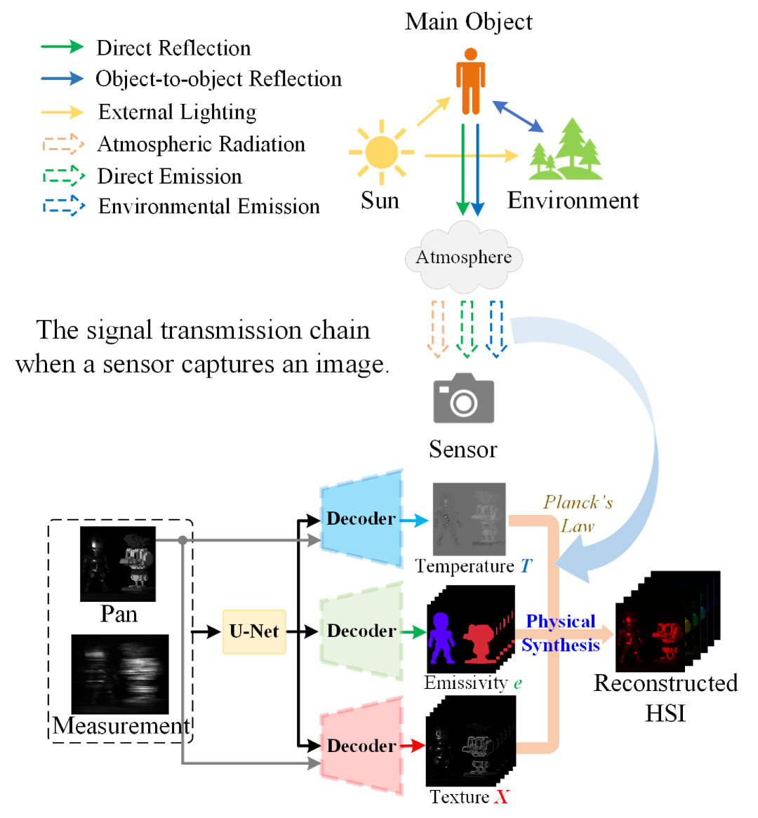
Figure 1: Our physics-informed HSI reconstruction method.

Traditional methods utilize hand-designed priors for reconstruction, such as sparsity lin2014spatial ; wang2016simultaneous , non-local similarity fu2016exploiting ; he2020non , low-rank liu2018rank , and total variation kittle2010multiframe ; wang2015dual . However, these methods require manual adjustment of the parameters, which often leads to mismatches between the prior assumptions and the actual problem. In deep learning-based methods, end-to-end methods yuan2018hyperspectral ; meng2020end treat the HSI reconstruction process as a black box, learning the transformation that maps spatial and spectral information to reconstructed HSIs. Additionally, some deep unfolding methods cai2022degradation ; li2023pixel attempt to incorporate physical priors into model training to enhance the model’s interpretability. The prior modules in these methods typically require a denoiser for multi-stage optimization, which is designed to effectively utilize both spatial and spectral information. However, in the aforementioned methods, researchers primarily focus on explicitly learning spatial and spectral information, often overlooking the physical imaging process of HSI bao2023heat . This has led to a bottleneck in HSI reconstruction.

In recent years, vision Transformer (ViT)-based HSI reconstruction methods cai2022mask ; li2023pixel ; yao2024specat have emerged due to their capability to capture global dependencies and non-local similarities. However, due to the significantly higher dimensionality of HSI data compared to traditional RGB images, the computational complexity of ViT grows quadratically with the increase in input sequence length. Visual Mamba (VMamba) models sequential dependencies by dividing an image into sequential blocks while maintaining linear computational complexity liu2025vmamba . This approach has been widely applied in various fields, including remote sensing image segmentation zhu2024samba ; cao2024remote , multimodal detection ren2024remotedet , and image super-resolution qiao2024hi ; ren2024mambacsr . However, VMamba assumes that the relationships between input sequences diminish as the sequential distance increases, which limits the ability to learn compact correlations between multimodal information. In addition, VMamba’s pixel-wise scanning of high-dimensional data imposes a heavy computational burden, leading to significant resource consumption.

To address the issues mentioned above, we propose a physics-informed cross-modal state space model (SSM) network (PCMamba) for DCCHI. PCMamba integrates the physical imaging process of hyperspectral signals with the linear complexity advantage of Mamba, effectively enhancing the quality of HSI reconstruction while preserving a lightweight computational cost. Specifically, we first analyze the physical process involved when the sensor captures spectral signals, as shown in Fig. 1. The thermal signals produced by an object in a specific band stem from both its own direct thermal emission and the environmental emission of surrounding objects. The former is governed by Planck’s law, the object’s temperature, and its emissivity, while the latter encapsulates the primary texture information in the HSI. Both signals are captured by the sensor after propagating through the atmosphere. Motivated by this observation, we aim to disentangle the object’s temperature, emissivity, and texture, and subsequently reconstruct the HSI through a physical synthesis process. This physics-informed feature learning approach fully utilizes the latent information embedded in 2D compressed measurements and PAN images, moving beyond the sole reliance on explicit spectral and spatial information. To achieve this goal, we design a Cross-Modal Scanning Mamba Block (CSMB) that performs inter-modal cross-scanning between the backbone features and PAN features, without pixel position repetition. This scanning scheme reduces the sequence length by half, while encouraging the model to learn more compact pixel-wise inter-modal interactions with a positional inductive bias.

Our contributions can be summarized as follows:

• We propose PCMamba, a physics-informed cross-modal SSM network for DCCHI. PCMamba integrates the linear complexity of Mamba with the forward physical imaging process of HSI, enabling both lightweight and high-quality HSI reconstruction.

• This is the first attempt to tackle the DCCHI task from the perspective of HSI thermal signal imaging, aiming to overcome the existing bottleneck in HSI reconstruction by exploring the latent physical properties embedded in the input image.

• We design a Cross-Modal Scanning Mamba Block (CSMB) that performs cross-scanning of features from different modalities without overlapping pixel positions. This design shortens the sequence length processed by the model and enhances its ability to learn more compact inter-modal associations.

• Experiments on both real and simulated datasets demonstrate the effectiveness and efficiency of the proposed method. Ablation studies further validate the contribution of each module.

2 Related Work

2.1 DCCHI System

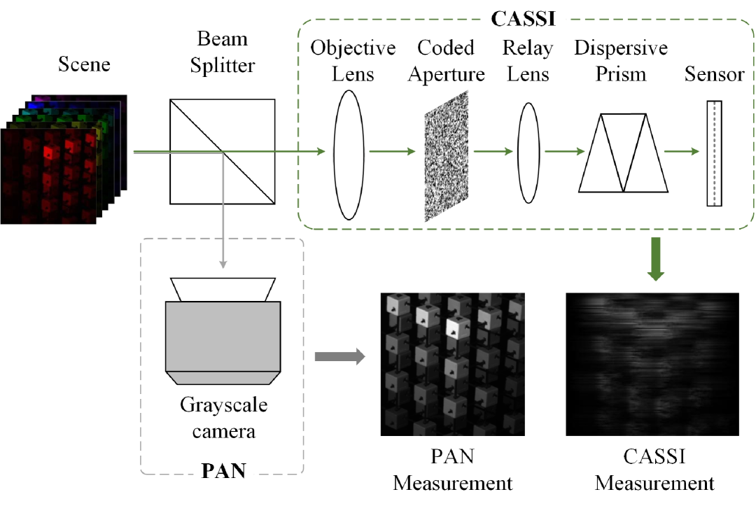
Figure 2: The dual-camera compressive hyperspectral imaging system.

The principle of DCCHI is shown in Fig. 2, which consists of a beam splitter, a PAN camera branch and a CASSI branch. The beam splitter splits the incident light equally in two directions, one direction is captured by the CASSI branch, which compresses the 3D HSI cube into a measurement by spatial and spectral modulation, and the other direction is captured by the PAN camera branch to generate a grayscale measurement.

The measurement $\mathbf{y^{c}}$ obtained by CASSI branch modulation can be formulated as

$$\mathbf{y^{c}}=\mathbf{\Phi^{c}}\mathbf{x}+\mathbf{g^{c}},$$ (1)

where $\mathbf{x}$ is the 3D HSI cube of the target scene, $\Phi^{c}$ is the coded aperture, and $\mathbf{g^{c}}$ is the Gaussian noise generated during the imaging process. Likewise, the imaging model of the PAN camera branch can be described as

$$\mathbf{y^{P}}=\mathbf{\Phi^{P}}\mathbf{x}+\mathbf{g^{P}},$$ (2)

To faciliate the subsequent discussion of the imaging model, we define $\mathbf{y}$, $\mathbf{\Phi}$, $\mathbf{g}$ as

$$\mathbf{y}=\begin{bmatrix}\mathbf{y^{c}}\\ \mathbf{y^{P}}\end{bmatrix},\mathbf{\Phi}=\begin{bmatrix}\mathbf{\Phi^{c}}\\ \mathbf{\Phi^{P}}\end{bmatrix},\mathbf{g}=\begin{bmatrix}\mathbf{g^{c}}\\ \mathbf{g^{P}}\end{bmatrix},$$ (3)

Based on the above definition, the imaging model of DCCHI can be expressed as

$$\mathbf{y}=\mathbf{\Phi}\mathbf{x}+\mathbf{g}.$$ (4)

2.2 Traditional HSI reconstruction methods

Traditional HSI reconstruction methods are mainly relied on hand-crafted priors yuan2016generalized ; liu2018rank ; he2020non . For example, GAP-TV yuan2016generalized introduces a generalized alternating projection algorithm using total variation minimization. Twist bioucas2007new proposes a two-step iterative shrinkage / thresholding algorithm for reconstructing missing samples. Non-local similarity and low-rank regularization fu2016exploiting ; liu2018rank ; he2020non are applied to explore spatial and spectral correlations. Sparse representation lin2014spatial ; arguello2013higher ; wang2016simultaneous models image sparsity by learning complete dictionaries. In  yang2014compressive , the image is reconstructed by learning a Gaussian mixture model of the signal. However, these model-driven methods lack efficiency and flexibility due to the need for manual tuning of extensive parameters.

2.3 Deep Learning-based DCCHI Methods

Using PAN to assist HSI reconstruction can effectively address the inherent limitations of CASSI. PFusion he2021fast uses RGB measurements to estimate the spatial coefficients and employs CASSI measurements to provide the spectral basis, thereby exploring the low-dimensional spectral subspace property of the HSI, which consists of spectral basis and spatial coefficients. PIDS chen2023prior utilizes the RGB image as a prior image to provide valuable semantic information. In2SET Wang_2024_CVPR employs a novel attention mechanism to capture both intra-similarity and inter-similarity between spectral and PAN images. Besides, some ViT-based methods attempt to recover HSI from a single measurement. MST cai2022mask utilizes transformer to capture the inter-spectral similarity of HSI. DAUHST cai2022degradation customizes a Half-Shuffle Transformer to capture both local content and non-local dependencies. PADUT li2023pixel proposes the nonlocal spectral transformer for modeling spatial and spectral similarity at a fine-grained level. SPECAT yao2024specat uses Swintransformer liu2021swin to model spatial sparsity. These methods show superior performance on HSI reconstruction than previous methods. However, these methods focus on explicitly exploring spatial and spectral information, while neglecting the underlying physical properties of HSI.

3 Method

Fig. 3 illustrates the overall architecture of our proposed PCMamba, which consists of two parts: a state space model (SSM) network with a U-net architecture composed of Cross-Modal Scanning Mamba Blocks (CSMBs), and the physical synthesis process of the HSI. The details are illustrated as below.

3.1 TeX decomposition

During the process of capturing hyperspectral signals, the sensor mixes the temperature (T, physical status), emissivity (e, material fingerprint), and texture of the object (X, surface geometry) in the photon flux bao2023heat . These physical properties collectively contribute to both the direct emission of the primary target and the environmental emission from surrounding objects.

$$\mathcal{S}_{\lambda}^{\alpha}=\Phi_{\lambda}^{\alpha}+\Psi_{\lambda}^{\alpha},$$ (5)

where $\Phi_{\lambda}^{\alpha}$ is the direct emission from the object $\alpha$ at wavelength $\lambda$, and $\Psi_{\lambda}^{\alpha}$ is environmental emission. Furthermore, the direct emission $\Phi_{\lambda}^{\alpha}$ consists of two components: the blackbody radiation of the object $\alpha$, governed by Planck’s law, and its emissivity.

$$\Phi_{\lambda}^{\alpha}=\mathit{e}_{\lambda}^{\alpha}B_{\lambda}\left(T\right),$$ (6)

$$B_{\lambda}\left(T\right)=\frac{2\pi hc^{2}}{\lambda^{5}}\frac{1}{e^{\frac{hc}{\lambda kT}}-1},$$ (7)

where $\emph{e}_{\lambda}^{\alpha}$ represents the emissivity of the object $\alpha$ at wavelength $\lambda$, and $B_{\lambda}\left(T\right)$ represents its blackbody radiation. Eq. (7) is Planck’s law, where $h$ is Planck constant, $k$ is Boltzmann constant, and $c$ is the speed of light. It is evident that the blackbody radiation of an object is solely determined by its wavelength $\lambda$ and temperature T.

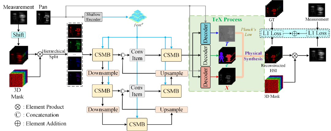
Figure 3: Overview of PCMamba. PCMamba consists of a state space model network with a U-net architecture composed of Cross-Modal Scanning Mamba Blocks (CSMB), and the physical synthesis process of the HSI, which combines Planck’s law and TeX decomposition.

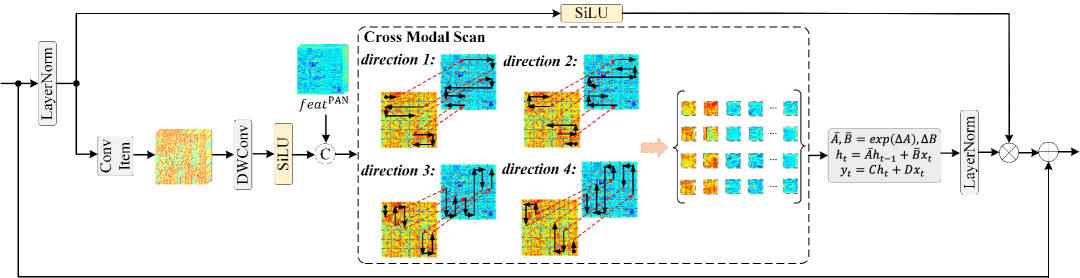
Figure 4: Illustration of Cross-Modal Scanning Mamba Block (CSMB). CSMB performs non-overlapping cross-scanning between backbone features and PAN features to learn more compact inter-modal correlations.

An important fact is that the surface texture of the object is obscured by its direct thermal emission, a phenomenon known as the “ghosting effect” gurton2014enhanced . The structural information observed in the image primarily comes from external light sources and environmental emissions, as shown in Fig. 1. Therefore, to fully describe the hyperspectral signal, it is necessary to consider the emission contributed by the environment. Given the emissivity $\emph{e}_{\lambda}^{\alpha}$ of object $\alpha$ at wavelength $\lambda$, its corresponding environmental emission $\Psi_{\lambda}^{\alpha}$ can be calculated as

$$\Psi_{\lambda}^{\alpha}=\left(1-e_{\lambda}^{\alpha}\right)X_{\lambda}^{\alpha},$$ (8)

$$X_{\lambda}^{\alpha}=\sum_{i=1}^{N-1}V_{\alpha\beta_{i}}\mathcal{S}_{\lambda}^{\beta_{i}},$$ (9)

where $\beta_{i}$ is the $i$-th object surrounding $\alpha$, and $V_{\alpha\beta_{i}}$ represents the linear combination vector between $\beta_{i}$ and $\alpha$. $\Psi$ represents multiple reflections between objects and contains the main texture information.

Furthermore, the hyperspectral signals, after passing through the atmosphere, are transmitted to the sensor along with atmospheric radiation

$$\mathcal{T}=\gamma\mathcal{S}+\left(1-\gamma\right)\Lambda,$$ (10)

where $\gamma$ represents the transmissivity of atmosphere Incropera_DeWitt_Bergman_Lavine_2018 , $\Lambda$ is atmospheric radiation, and $\mathcal{T}$ represents the total radiation signal.

Finally, the hyperspectral signal captured by the sensor can be rewritten as

$$\mathcal{T}=\gamma\left(\mathit{e}_{\lambda}B_{\lambda}\left(T\right)+\left(1-e_{\lambda}\right)X_{\lambda}\right)+\left(1-\gamma\right)\Lambda,$$ (11)

Due to the absorption of spectral signals by water vapor and carbon dioxide in the atmosphere, $\gamma$ is typically close to 1, resulting in the approximation of $\mathcal{T}$ as

$$\mathcal{T}=\mathit{e}_{\lambda}B_{\lambda}\left(T\right)+\left(1-e_{\lambda}\right)X_{\lambda}.$$ (12)

This implies that the HSI can be synthesized through a forward physical process if the temperature $T$, emissivity $e$, and texture $X$ can be accurately obtained.

3.2 Hyperspectral Signals

For HSIs, the spectral signals captured at wavelength $\lambda$ is equal to the superimposition of signals over the entire wavelength range [$\lambda_{min}$, $\lambda_{max}$]

$$\int_{\lambda_{min}}^{\lambda_{max}}\mathcal{S}_{\lambda}^{\alpha}d\lambda =\int_{\lambda_{min}}^{\lambda_{max}}e_{\lambda}^{\alpha}B_{\lambda}^{\alpha}\left(T\right)d\lambda$$ (13)

$$+\int_{\lambda_{min}}^{\lambda_{max}}\left(1-e_{\lambda}^{\alpha}\right)\sum_{i=1}^{N-1}V_{\alpha\beta_{i}}\mathcal{S}_{\lambda}^{\beta_{i}}d\lambda,$$

Available data in bao2023heat indicates that, the emissivity $e_{\lambda}$ of most objects remains relatively constant across the short working wavelengths. Therefore, we assume a constant emissivity for a specific material

$$\int_{\lambda_{min}}^{\lambda_{max}}\mathcal{S}_{\lambda}^{\alpha}d\lambda =e_{\lambda}^{\alpha}\int_{\lambda_{min}}^{\lambda_{max}}B_{\lambda}^{\alpha}\left(T\right)d\lambda$$ (14)

$$+\left(1-e_{\lambda}^{\alpha}\right)\int_{\lambda_{min}}^{\lambda_{max}}\sum_{i=1}^{N-1}V_{\alpha\beta_{i}}\mathcal{S}_{\lambda}^{\beta_{i}}d\lambda.$$

3.3 Cross-Modal Scanning Mamba Block (CSMB)

SSM utilizes a framework of linear ordinary differential equations to map inputs to outputs through hidden state. For a system with input excitation $x(t)\in\mathbb{R}^{L}$, hidden state $h(t)\in\mathbb{C}^{N}$ and output response $y(t)\in\mathbb{R}^{L}$, the model can be formulated as

$$h^{\prime}(t)=\mathbf{A}h(t)+\mathbf{B}x(t),$$ (15)

$$y(t)=\mathbf{C}h(t)+\mathbf{D}x(t),$$

where $\mathbf{A}\in\mathbb{C}^{N\times N}$, $\mathbf{B},\mathbf{C}\in\mathbb{C}^{N}$ and $\mathbf{D}\in\mathbb{C}^{1}$ are weighting parameters. Subsequently, a discretization of Eq. (15) is usually obtained using a zero-order keeper (ZOH)

$$\begin{array}[]{c}\overline{\mathbf{A}}=\exp(\Delta\mathbf{A}),\\ \overline{\mathbf{B}}=(\Delta\mathbf{A})^{-1}(\exp(\Delta\mathbf{A})-I)\cdot\Delta\mathbf{B},\end{array}$$ (16)

where $\Delta$ is a time scale parameter used to transform the continuous parameters $\mathbf{A}$, $\mathbf{B}$ into discrete parameters $\overline{\mathbf{A}}$, $\overline{\mathbf{B}}$. The discretized Eq. (15) can be written as

$$h_{t}=\overline{\mathbf{A}}h_{t-1}+\overline{\mathbf{B}}x_{t},$$ (17)

$$y_{t}=\mathbf{C}h_{t}+\mathbf{D}x_{t},$$

Given that the dimensionality of HSI data is several orders of magnitude higher than that of conventional RGB image, we adopt the SSM with linear complexity to keep the network lightweight. We aim to facilitate effective interaction between information from compressed measurements and PAN images, while mitigating interference from redundant spectral information. We first employ a shallow encoder to extract multi-scale PAN features

$$\left[feat_{1}^{P},feat_{2}^{P},\cdots,feat_{M}^{P}\right]=\mathrm{SE}\left(P\right),$$ (18)

where $P$ denotes a PAN image, SE($\cdot$) is a shallow encoder, and the subscript $M$ denotes the PAN features at different scales. Similarly, the backbone features are represented as $feat_{N}^{B}$. Then we ensure that $feat_{k}^{P}$ and $feat_{k}^{B}$ have the same spatial size and perform cross-scanning on them without pixel position overlap, as shown in Fig. 4

$$feat^{\mathrm{B}}_{k+1} =\mathrm{CS}\left(\mathrm{LN}\left(feat^{B}_{k}\right),feat^{P}_{k}\right)\odot$$ (19)

$$\mathrm{SiLU}\left(\mathrm{LN}\left(feat^{B}_{k}\right)\right)+feat^{\mathrm{B}}_{k}.$$

where $\operatorname{CS\left(\cdot\right)}$ represents the cross-modal scanning operation which employs the following operation sequence: $DWConv\to SiLU\to SSM\to LN$. This non-overlapping pixel position scanning method helps to suppress redundant spectral information between bands, encourages the network to learn a more compact pixel-wise inductive bias between emissivity and texture, and simultaneously reduces the sequence length processed by the SSM by half.

Finally, three decoders are applied to the output features of the U-net to generate the desired temperature T, emissivity e, and texture X. Since the PAN image theoretically shares the same temperature properties as the measurement, we leverage it to facilitate the generation of T. Likewise, the PAN is utilized to inject additional structural details into the generation of X, as shown in Fig. 3.

3.4 Loss Function

In this paper, we use L1 loss to optimize the reconstructed HSI at the pixel level

$$\begin{split}\mathcal{L}_{Rec}=\frac{1}{H\times W\times C}\sum_{i=0}\left|\widehat{Y}\left(i\right)-Y\left(i\right)\right|,\end{split}$$ (20)

where $C$ is the number of channels in the reconstructed HSI, $\widehat{Y}\left(i\right)$ represents the predicted value for pixel $i$, and $Y\left(i\right)$ is its corresponding ground truth. Besides, we ensure the rationality of the entire reconstruction process by modulating the reconstruction result of PCMamba to generate a 2D measurement consistent with the network input

$$\begin{gathered}\mathcal{L}_{\mathcal{M}}={\left\|\mathcal{M}\odot\widehat{Y}-\mathcal{X}\right\|}^{2}_{1},\end{gathered}$$ (21)

where $\mathcal{M}$ is the modulated mask and $\mathcal{X}$ is the input 2D measurement. The total loss $\mathcal{L}_{total}$ is defined by combing the reconstruction loss $\mathcal{L}_{Rec}$ and the imaging process consistency loss $\mathcal{L}_{\mathcal{M}}$

$$\begin{gathered}\mathcal{L}_{total}=\mathcal{L}_{Rec}+\mathcal{L}_{\mathcal{M}}.\end{gathered}$$ (22)

Table 1: Comparison of different methods on 10 simulated scenes including FLOPS, PSNR (upper entry) and SSIM (lower entry). “Method-RGB” denotes the use of RGB observations, and “Method-PAN” denotes grayscale observations in the PAN image. Notably, “Method-PAN” is modified from other HSI reconstruction methods in the DCCHI reconstruction task. The best values are bolded.

Methods	GFLOPs	Scene1	Scene2	Scene3	Scene4	Scene5	Scene6	Scene7	Scene8	Scene9	Scene10	Avg
PFsion-RGB he2021fast	-	40.09 0.979	38.84 0.968	38.70 0.966	46.65 0.936	32.07 0.980	37.12 0.980	39.74 0.964	36.75 0.965	34.52 0.931	35.53 0.979	38.00 0.965
PIDS-RGB chen2023prior	-	42.09 0.983	40.08 0.949	41.50 0.968	48.55 0.989	40.05 0.982	39.00 0.974	36.63 0.940	37.02 0.948	38.82 0.953	38.64 0.980	40.24 0.967
TV-PAN wang2015dual	-	35.81 0.947	33.22 0.885	31.07 0.879	40.11 0.947	33.32 0.944	34.62 0.943	31.09 0.885	32.31 0.916	29.36 0.862	33.84 0.953	33.47 0.910
PIDS-PAN chen2023prior	-	39.82 0.977	37.07 0.921	37.72 0.950	46.78 0.978	37.45 0.973	37.74 0.963	32.90 0.896	31.66 0.915	34.35 0.902	38.58 0.972	37.41 0.945
BiSRNet-PAN cai2024binarized	1.33	35.02 0.945	34.13 0.914	31.50 0.883	35.88 0.895	33.70 0.935	35.58 0.925	32.31 0.900	32.73 0.903	31.37 0.899	34.48 0.936	33.67 0.914
CST-PAN cai2022coarse	25.40	37.44 0.975	38.91 0.978	36.79 0.969	42.27 0.983	36.57 0.982	38.91 0.984	36.87 0.967	35.91 0.980	35.87 0.973	37.93 0.990	37.75 0.978
HDNet-PAN hu2022hdnet	144.31	38.06 0.976	39.79 0.982	38.21 0.973	42.79 0.983	37.22 0.983	39.26 0.986	37.41 0.968	36.51 0.982	36.64 0.976	37.52 0.988	38.34 0.980
MST++-PAN cai2022mst++	17.69	38.38 0.977	40.47 0.980	37.70 0.968	43.88 0.984	37.75 0.983	39.42 0.985	37.48 0.964	37.38 0.982	38.82 0.980	39.04 0.989	39.03 0.980
DAUHST-PAN-2stg cai2022degradation	16.79	40.78 0.983	43.13 0.987	41.73 0.980	47.09 0.990	39.84 0.987	40.90 0.986	39.75 0.976	38.98 0.981	41.29 0.983	40.04 0.988	40.22 0.983
DAUHST-PAN-3stg cai2022degradation	24.70	40.22 0.983	43.52 0.989	41.74 0.981	47.07 0.993	38.81 0.985	40.16 0.987	39.86 0.978	38.21 0.981	40.63 0.983	39.32 0.990	40.95 0.985
DAUHST-PAN-5stg cai2022degradation	40.51	40.74 0.984	44.00 0.989	41.58 0.981	46.84 0.991	39.66 0.986	40.89 0.987	40.21 0.979	38.72 0.983	39.98 0.982	40.10 0.989	41.27 0.916
DAUHST-PAN-9stg cai2022degradation	72.11	41.59 0.985	45.19 0.991	43.47 0.984	48.92 0.993	40.27 0.988	41.17 0.988	40.73 0.979	40.11 0.986	43.50 0.988	41.33 0.990	42.62 0.987
In2SET-2stg Wang_2024_CVPR	14.35	40.33 0.983	42.30 0.985	40.34 0.977	47.24 0.991	39.42 0.986	40.61 0.986	39.46 0.975	38.42 0.979	40.37 0.981	39.96 0.988	40.84 0.983
In2SET-3stg Wang_2024_CVPR	20.79	40.78 0.983	43.13 0.987	41.73 0.980	47.09 0.990	39.84 0.987	40.90 0.986	39.75 0.976	38.98 0.981	41.29 0.983	40.04 0.988	41.35 0.984
In2SET-5stg Wang_2024_CVPR	33.66	41.13 0.985	44.43 0.990	42.74 0.983	47.29 0.993	40.33 0.988	40.95 0.987	40.49 0.979	39.15 0.982	42.07 0.985	39.44 0.987	41.80 0.985
In2SET-9stg Wang_2024_CVPR	59.40	42.56 0.989	46.42 0.994	44.55 0.986	50.63 0.996	42.01 0.992	42.49 0.991	41.59 0.983	40.53 0.989	43.83 0.990	42.33 0.994	43.69 0.990
SPECAT-PAN yao2024specat	12.40	43.02 0.991	45.79 0.994	44.04 0.985	47.09 0.993	41.56 0.993	44.32 0.994	42.25 0.986	43.15 0.993	43.65 0.991	43.19 0.994	43.81 0.991
Ours	18.91	43.35 0.994	47.16 0.997	44.71 0.988	47.46 0.996	41.75 0.995	45.35 0.997	43.73 0.990	43.98 0.996	44.02 0.993	43.19 0.997	44.47 0.994

4 Experiments

4.1 Experimental Settings

Dataset. We used two simulated hyperspectral datasets: CAVE yasuma2010generalized , KAIST choi2017high and one real dataset wang2016adaptive . The CAVE dataset contains 32 hyperspectral images with a spatial resolution of 512$\times$512 pixels. The KAIST dataset consists of 30 hyperspectral images with a higher spatial resolution of 2704$\times$3306 pixels and a spectral dimension of 31. Following the protocol established in previous works cai2022mask ; huang2021deep ; Wang_2024_CVPR , we used the CAVE dataset for training set and select a subset of 10 scene crops from the KAIST dataset along with the real dataset for testing.

Implementation Details. We implemented our network on the PC with a single NVIDIA RTX 4090 GPU and built it in the PyTorch framework. In the training phase, the Adam optimizer diederik2014adam was used to optimize the model parameters. The initial learning rate was set to $4\times 10^{-4}$ , and the learning rate was decayed using a cosine annealing schedule with a minimum value of $1\times 10^{-6}$. The batch size was set to 4. We cropped $256\times 256$ patches from 3D cubes and input them into the network.

4.2 Baseline Methods

We compared our approach with three classic model-based spectral reconstruction methods (PFusion he2021fast , PIDS chen2023prior and TV wang2015dual ), five end-to-end methods (BiSRNet cai2024binarized , CST cai2022coarse , HDNet hu2022hdnet , MST++ cai2022mst++ and SPECAT yao2024specat ) and two depth unfolding methods (DAUHST cai2022degradation , In2SET Wang_2024_CVPR ).

4.3 Metrics

The reconstruction quality of hyperspectral images is evaluated using peak signal-to-noise ratio (PSNR) and structural similarity index (SSIM) metrics.

4.4 Simulation and Real Data Results

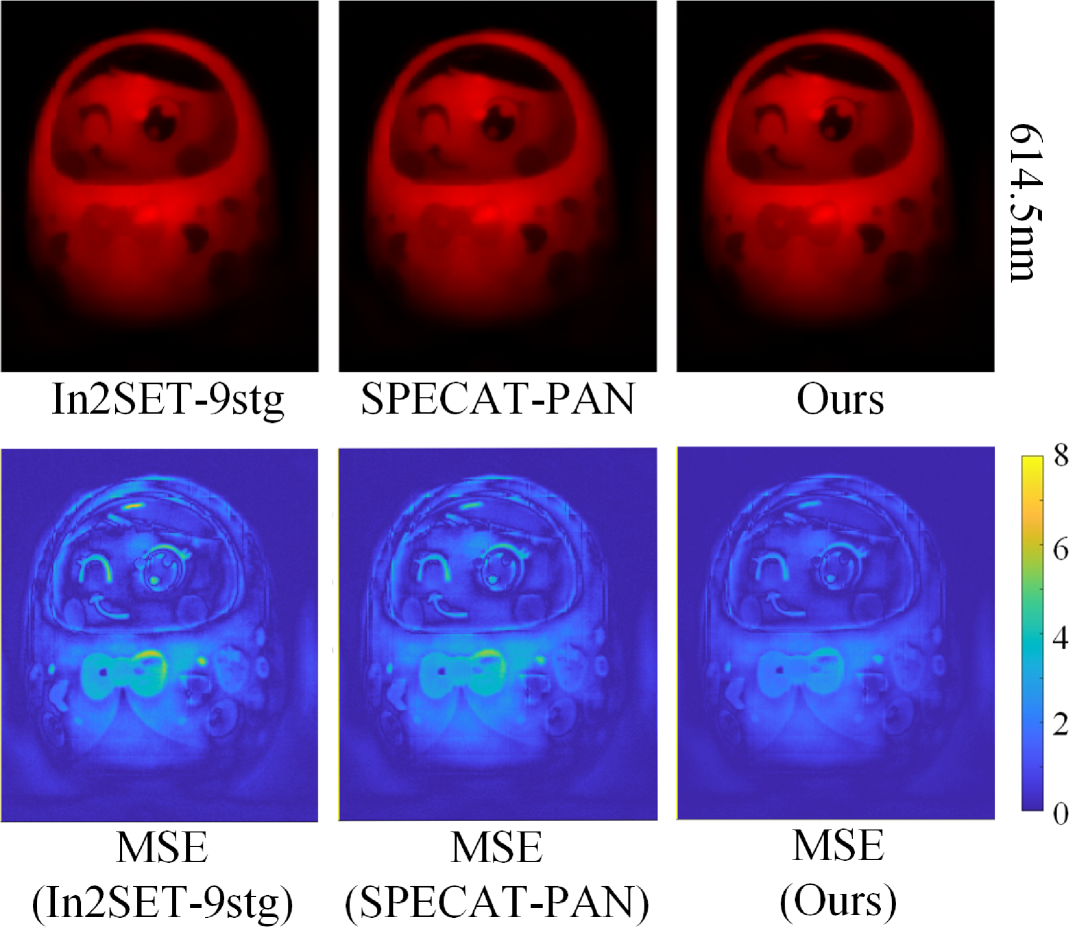
Figure 5: The visual comparisons between our method and SOTA methods on real dataset.

Numerical Results. The metrics of different methods on ten simulated scenes are shown in Tab. 1. Our method achieves superior performance in most scenes. The average PSNR and average SSIM of our method achieve 44.47 dB and 0.994, outperforming the second-best results by 0.66 dB and 0.003, respectively. Additionally, it can be observed that, compared to DAUHST-PAN-9stg and In2SET-9stg, PCMamba achieves higher reconstruction quality while requiring less than half of the computational cost.

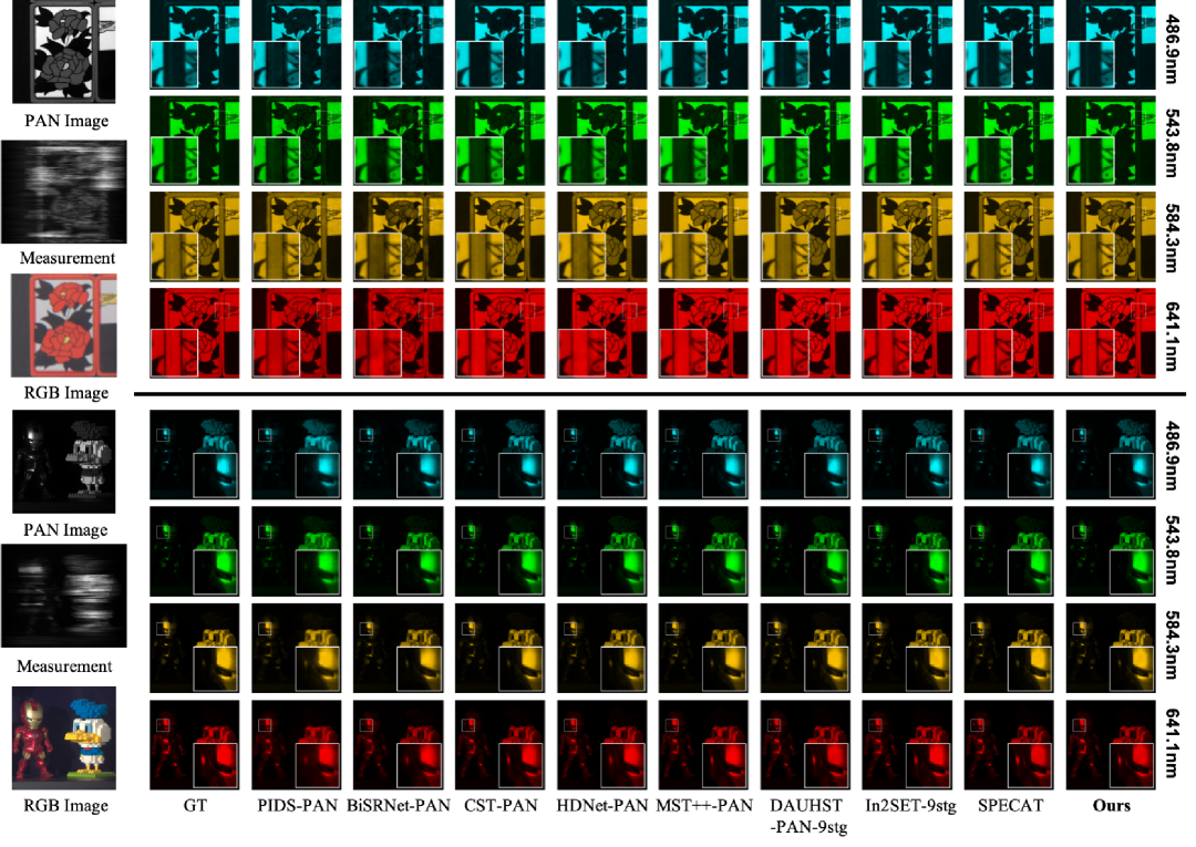
Figure 6: Comparison of the reconstruction results of different methods on two scenes from the KAIST dataset, including eight SOTA methods and our PCMamba. We select four bands (486.9 nm, 543.8 nm, 584.3 nm, and 641.1 nm) for visualization.

Visual Results. Fig. 5 shows the MSE residues between the reconstruction results and the ground truth on the real dataset, demonstrating that PCMamba achieves better spectral fidelity. To facilitate visual evaluation, we presented the reconstruction results of eight SOTA methods across four bands from the simulated dataset, alongside the ground truth. Fig. 6 illustrates these reconstruction results. By zooming into local regions, it can be observed that our method reconstructs results that are closer to the ground truth. For example, the vertical line to the left of the bird in the first image is restored more sharply by our method compared to other SOTA methods.

4.5 Ablation Study

TeX decomposition and the Cross-Modal Scanning Mamba Block (CSMB) are two key modules of PCMamba. We further conducted ablation experiments on simulated datasets to verify their effectiveness.

Table 2: Ablation studies on simulated dataset. ‘w/o’ denotes without, and ‘w/’ denotes with.

(a) Ablation studies of the TeX decomposition.

TeX Process	PSNR$\uparrow$	SSIM$\uparrow$
w/o TeX	43.65	0.991
w/ TeX	44.47	0.994

(b) Ablation studies of the Cross-Scan.

Cross-Scan	PSNR$\uparrow$	SSIM$\uparrow$
w/o	42.56	0.988
BFR = 0.3	44.03	0.993
BFR = 0.5	44.25	0.993
BFR = 0.7	44.47	0.994
BFR = 0.8	44.36	0.993
BFR = 0.9	44.20	0.993

(c) Ablation studies of the loss function terms.

Config	PSNR$\uparrow$	SSIM$\uparrow$
w/o $\mathcal{L}_{Rec}$	17.29	0.165
w/o $\mathcal{L}_{\mathcal{M}}$	44.08	0.993
Ours	44.47	0.994

TeX Decomposition.

As shown in Tab. 2 (a), we explored the impact of the introduced physical process on HSI reconstruction. Specifically, we removed the three decoders at the end of the U-net and directly generated the HSI. It is observed that the introduction of the TeX decomposition process improves PSNR by 0.82 dB, demonstrating that exploring the correlations between the latent physical properties within the input image is beneficial.

Cross-Modal Scanning Mamba Block (CSMB).

To validate the effectiveness of the cross-scanning scheme in CSMB, we replaced it with a Vanilla scan that performs pixel-wise scanning of both the backbone and PAN features. As shown in Tab. 2 (b), the cross-scanning scheme improved the PSNR by 1.91 dB, highlighting its effectiveness. Furthermore, we explored the impact of the backbone feature ratio (BFR) in the cross-scanning process. BFR is the proportion of backbone features in the encoder-decoder features. We found that maintaining an appropriate proportion between the backbone features and PAN features effectively enhanced the HSI reconstruction performance.

Loss Function.

We verified the effectiveness of each loss function by removing them individually, where the quantitative results are reported in Tab. 2 (c). It can be observed that the reconstruction loss $\mathcal{L}_{Rec}$ plays a major role, as it contains the primary supervisory information. On the other hand, the imaging process consistency loss $\mathcal{L}_{\mathcal{M}}$ effectively constrains the HSI generation process, resulting in an improvement in the quantitative metrics.

5 Conclusion

In this paper, we propose PCMamba, a physics-informed cross-modal SSM network for DCCHI. This is the first attempt to address the HSI reconstruction problem from the perspective of the physical process of spectral signal generation, aiming to provide theoretical guidance for future hyperspectral imaging tasks. PCMamba achieves the physical synthesis of HSI by exploiting three physical properties: temperature, emissivity, and texture. In addition, we design a Cross-Modal Scanning Mamba Block (CSMB), which learns more compact inter-modal inductive biases by performing cross-scanning without positional overlap across different modality features, thereby significantly reducing the computational cost of the SSM. Extensive experiments conducted on both real and simulated datasets demonstrate the effectiveness and efficiency of our method.

References

- [1] Gonzalo R Arce, David J Brady, Lawrence Carin, Henry Arguello, and David S Kittle. Compressive coded aperture spectral imaging: An introduction. IEEE Signal Processing Magazine, 31(1):105–115, 2013.
- [2] Henry Arguello, Hoover Rueda, Yuehao Wu, Dennis W Prather, and Gonzalo R Arce. Higher-order computational model for coded aperture spectral imaging. Applied optics, 52(10):D12–D21, 2013.
- [3] Fanglin Bao, Xueji Wang, Shree Hari Sureshbabu, Gautam Sreekumar, Liping Yang, Vaneet Aggarwal, Vishnu N Boddeti, and Zubin Jacob. Heat-assisted detection and ranging. Nature, 619(7971):743–748, 2023.
- [4] José M Bioucas-Dias and Mário AT Figueiredo. A new twist: Two-step iterative shrinkage/thresholding algorithms for image restoration. IEEE Transactions on Image processing, 16(12):2992–3004, 2007.
- [5] Yuanhao Cai, Jing Lin, Xiaowan Hu, Haoqian Wang, Xin Yuan, Yulun Zhang, Radu Timofte, and Luc Van Gool. Coarse-to-fine sparse transformer for hyperspectral image reconstruction. In European conference on computer vision, pages 686–704. Springer, 2022.
- [6] Yuanhao Cai, Jing Lin, Xiaowan Hu, Haoqian Wang, Xin Yuan, Yulun Zhang, Radu Timofte, and Luc Van Gool. Mask-guided spectral-wise transformer for efficient hyperspectral image reconstruction. In Proceedings of the IEEE/CVF conference on computer vision and pattern recognition, pages 17502–17511, 2022.
- [7] Yuanhao Cai, Jing Lin, Zudi Lin, Haoqian Wang, Yulun Zhang, Hanspeter Pfister, Radu Timofte, and Luc Van Gool. Mst++: Multi-stage spectral-wise transformer for efficient spectral reconstruction. In Proceedings of the IEEE/CVF Conference on Computer Vision and Pattern Recognition, pages 745–755, 2022.
- [8] Yuanhao Cai, Jing Lin, Haoqian Wang, Xin Yuan, Henghui Ding, Yulun Zhang, Radu Timofte, and Luc V Gool. Degradation-aware unfolding half-shuffle transformer for spectral compressive imaging. Advances in Neural Information Processing Systems, 35:37749–37761, 2022.
- [9] Yuanhao Cai, Yuxin Zheng, Jing Lin, Xin Yuan, Yulun Zhang, and Haoqian Wang. Binarized spectral compressive imaging. Advances in Neural Information Processing Systems, 36, 2024.
- [10] Yice Cao, Chenchen Liu, Zhenhua Wu, Wenxin Yao, Liu Xiong, Jie Chen, and Zhixiang Huang. Remote sensing image segmentation using vision mamba and multi-scale multi-frequency feature fusion. arXiv preprint arXiv:2410.05624, 2024.
- [11] Yurong Chen, Yaonan Wang, and Hui Zhang. Prior image guided snapshot compressive spectral imaging. IEEE Transactions on Pattern Analysis and Machine Intelligence, 45(9):11096–11107, 2023.
- [12] Inchang Choi, MH Kim, D Gutierrez, DS Jeon, and G Nam. High-quality hyperspectral reconstruction using a spectral prior. Technical report, 2017.
- [13] P Kingma Diederik. Adam: A method for stochastic optimization. (No Title), 2014.
- [14] Ying Fu, Yinqiang Zheng, Imari Sato, and Yoichi Sato. Exploiting spectral-spatial correlation for coded hyperspectral image restoration. In Proceedings of the IEEE Conference on Computer Vision and Pattern Recognition, pages 3727–3736, 2016.
- [15] Kristan P Gurton, Alex J Yuffa, and Gorden W Videen. Enhanced facial recognition for thermal imagery using polarimetric imaging. Optics letters, 39(13):3857–3859, 2014.
- [16] Wei He, Quanming Yao, Chao Li, Naoto Yokoya, Qibin Zhao, Hongyan Zhang, and Liangpei Zhang. Non-local meets global: An iterative paradigm for hyperspectral image restoration. IEEE Transactions on Pattern Analysis and Machine Intelligence, 44(4):2089–2107, 2020.
- [17] Wei He, Naoto Yokoya, and Xin Yuan. Fast hyperspectral image recovery of dual-camera compressive hyperspectral imaging via non-iterative subspace-based fusion. IEEE Transactions on Image Processing, 30:7170–7183, 2021.
- [18] Xiaowan Hu, Yuanhao Cai, Jing Lin, Haoqian Wang, Xin Yuan, Yulun Zhang, Radu Timofte, and Luc Van Gool. Hdnet: High-resolution dual-domain learning for spectral compressive imaging. In Proceedings of the IEEE/CVF Conference on Computer Vision and Pattern Recognition, pages 17542–17551, 2022.
- [19] Tao Huang, Weisheng Dong, Xin Yuan, Jinjian Wu, and Guangming Shi. Deep gaussian scale mixture prior for spectral compressive imaging. In Proceedings of the IEEE/CVF Conference on Computer Vision and Pattern Recognition, pages 16216–16225, 2021.
- [20] F.P. Incropera, DP. DeWitt, T.L. Bergman, and AdrienneS. Lavine. Principles of heat and mass transfer. Jun 2018.
- [21] Nirmal Keshava. Distance metrics and band selection in hyperspectral processing with applications to material identification and spectral libraries. IEEE Transactions on Geoscience and remote sensing, 42(7):1552–1565, 2004.
- [22] Muhammad Jaleed Khan, Hamid Saeed Khan, Adeel Yousaf, Khurram Khurshid, and Asad Abbas. Modern trends in hyperspectral image analysis: A review. Ieee Access, 6:14118–14129, 2018.
- [23] David Kittle, Kerkil Choi, Ashwin Wagadarikar, and David J Brady. Multiframe image estimation for coded aperture snapshot spectral imagers. Applied optics, 49(36):6824–6833, 2010.
- [24] Miaoyu Li, Ying Fu, Ji Liu, and Yulun Zhang. Pixel adaptive deep unfolding transformer for hyperspectral image reconstruction. In Proceedings of the IEEE/CVF International Conference on Computer Vision, pages 12959–12968, 2023.
- [25] Yunsong Li, Yanzi Shi, Keyan Wang, Bobo Xi, Jiaojiao Li, and Paolo Gamba. Target detection with unconstrained linear mixture model and hierarchical denoising autoencoder in hyperspectral imagery. IEEE Transactions on Image Processing, 31:1418–1432, 2022.
- [26] Xing Lin, Yebin Liu, Jiamin Wu, and Qionghai Dai. Spatial-spectral encoded compressive hyperspectral imaging. ACM Transactions on Graphics (TOG), 33(6):1–11, 2014.
- [27] Tingting Liu, Hai Liu, You-Fu Li, Zengzhao Chen, Zhaoli Zhang, and Sannyuya Liu. Flexible ftir spectral imaging enhancement for industrial robot infrared vision sensing. IEEE Transactions on Industrial Informatics, 16(1):544–554, 2019.
- [28] Yang Liu, Xin Yuan, Jinli Suo, David J Brady, and Qionghai Dai. Rank minimization for snapshot compressive imaging. IEEE transactions on pattern analysis and machine intelligence, 41(12):2990–3006, 2018.
- [29] Yue Liu, Yunjie Tian, Yuzhong Zhao, Hongtian Yu, Lingxi Xie, Yaowei Wang, Qixiang Ye, Jianbin Jiao, and Yunfan Liu. Vmamba: Visual state space model. Advances in neural information processing systems, 37:103031–103063, 2025.
- [30] Ze Liu, Yutong Lin, Yue Cao, Han Hu, Yixuan Wei, Zheng Zhang, Stephen Lin, and Baining Guo. Swin transformer: Hierarchical vision transformer using shifted windows. In Proceedings of the IEEE/CVF international conference on computer vision, pages 10012–10022, 2021.
- [31] Patrick Llull, Xuejun Liao, Xin Yuan, Jianbo Yang, David Kittle, Lawrence Carin, Guillermo Sapiro, and David J Brady. Coded aperture compressive temporal imaging. Optics express, 21(9):10526–10545, 2013.
- [32] Ziyi Meng, Jiawei Ma, and Xin Yuan. End-to-end low cost compressive spectral imaging with spatial-spectral self-attention. In European conference on computer vision, pages 187–204. Springer, 2020.
- [33] Ziyi Meng, Mu Qiao, Jiawei Ma, Zhenming Yu, Kun Xu, and Xin Yuan. Snapshot multispectral endomicroscopy. Optics Letters, 45(14):3897–3900, 2020.
- [34] Junbo Qiao, Jincheng Liao, Wei Li, Yulun Zhang, Yong Guo, Yi Wen, Zhangxizi Qiu, Jiao Xie, Jie Hu, and Shaohui Lin. Hi-mamba: Hierarchical mamba for efficient image super-resolution. arXiv preprint arXiv:2410.10140, 2024.
- [35] Kejun Ren, Xin Wu, Lianming Xu, and Li Wang. Remotedet-mamba: A hybrid mamba-cnn network for multi-modal object detection in remote sensing images. arXiv preprint arXiv:2410.13532, 2024.
- [36] Yulin Ren, Xin Li, Mengxi Guo, Bingchen Li, Shijie Zhao, and Zhibo Chen. Mambacsr: Dual-interleaved scanning for compressed image super-resolution with ssms. arXiv preprint arXiv:2408.11758, 2024.
- [37] Michal Shimoni, Rob Haelterman, and Christiaan Perneel. Hypersectral imaging for military and security applications: Combining myriad processing and sensing techniques. IEEE Geoscience and Remote Sensing Magazine, 7(2):101–117, 2019.
- [38] Burak Uzkent, Aneesh Rangnekar, and Matthew Hoffman. Aerial vehicle tracking by adaptive fusion of hyperspectral likelihood maps. In Proceedings of the IEEE Conference on Computer Vision and Pattern Recognition Workshops, pages 39–48, 2017.
- [39] Lizhi Wang, Zhiwei Xiong, Dahua Gao, Guangming Shi, and Feng Wu. Dual-camera design for coded aperture snapshot spectral imaging. Applied optics, 54(4):848–858, 2015.
- [40] Lizhi Wang, Zhiwei Xiong, Hua Huang, Guangming Shi, Feng Wu, and Wenjun Zeng. High-speed hyperspectral video acquisition by combining nyquist and compressive sampling. IEEE transactions on pattern analysis and machine intelligence, 41(4):857–870, 2018.
- [41] Lizhi Wang, Zhiwei Xiong, Guangming Shi, Feng Wu, and Wenjun Zeng. Adaptive nonlocal sparse representation for dual-camera compressive hyperspectral imaging. IEEE transactions on pattern analysis and machine intelligence, 39(10):2104–2111, 2016.
- [42] Lizhi Wang, Zhiwei Xiong, Guangming Shi, Wenjun Zeng, and Feng Wu. Simultaneous depth and spectral imaging with a cross-modal stereo system. IEEE Transactions on Circuits and Systems for Video Technology, 28(3):812–817, 2016.
- [43] Xin Wang, Lizhi Wang, Xiangtian Ma, Maoqing Zhang, Lin Zhu, and Hua Huang. In2set: Intra-inter similarity exploiting transformer for dual-camera compressive hyperspectral imaging. In Proceedings of the IEEE/CVF Conference on Computer Vision and Pattern Recognition (CVPR), pages 24881–24891, June 2024.
- [44] Hui Xie, Zhuang Zhao, Jing Han, Yi Zhang, Lianfa Bai, and Jun Lu. Dual camera snapshot hyperspectral imaging system via physics-informed learning. Optics and Lasers in Engineering, 154:107023, 2022.
- [45] Jianbo Yang, Xuejun Liao, Xin Yuan, Patrick Llull, David J Brady, Guillermo Sapiro, and Lawrence Carin. Compressive sensing by learning a gaussian mixture model from measurements. IEEE Transactions on Image Processing, 24(1):106–119, 2014.
- [46] Zhiyang Yao, Shuyang Liu, Xiaoyun Yuan, and Lu Fang. Specat: Spatial-spectral cumulative-attention transformer for high-resolution hyperspectral image reconstruction. In Proceedings of the IEEE/CVF Conference on Computer Vision and Pattern Recognition, pages 25368–25377, 2024.
- [47] Fumihito Yasuma, Tomoo Mitsunaga, Daisuke Iso, and Shree K Nayar. Generalized assorted pixel camera: postcapture control of resolution, dynamic range, and spectrum. IEEE transactions on image processing, 19(9):2241–2253, 2010.
- [48] Qiangqiang Yuan, Qiang Zhang, Jie Li, Huanfeng Shen, and Liangpei Zhang. Hyperspectral image denoising employing a spatial–spectral deep residual convolutional neural network. IEEE Transactions on Geoscience and Remote Sensing, 57(2):1205–1218, 2018.
- [49] Xin Yuan. Generalized alternating projection based total variation minimization for compressive sensing. In 2016 IEEE International conference on image processing (ICIP), pages 2539–2543. IEEE, 2016.
- [50] Yuan Yuan, Xiangtao Zheng, and Xiaoqiang Lu. Hyperspectral image superresolution by transfer learning. IEEE Journal of Selected Topics in Applied Earth Observations and Remote Sensing, 10(5):1963–1974, 2017.
- [51] Qinfeng Zhu, Yuanzhi Cai, Yuan Fang, Yihan Yang, Cheng Chen, Lei Fan, and Anh Nguyen. Samba: Semantic segmentation of remotely sensed images with state space model. Heliyon, 10(19), 2024.