$\alpha+{}^{2}n+{}^{2}n$ 3-body cluster structures and dineutron breaking in ${}^{8}\mathrm{He}$

Abstract

Background

The $0_{2}^{+}$ state of ${}^{8}\mathrm{He}$ has been discovered by a recent experiment, which suggested a developed cluster structure of spatially correlated neutron pairs, called ”dineutrons” (${}^{2}n$).

Purpose

We aim to investigate the structure of ${}^{8}\mathrm{He}(0^{+}_{1})$ and ${}^{8}\mathrm{He}(0^{+}_{2})$ to clarify the monopole excitation mode in ${}^{8}\mathrm{He}$ system while focusing on the $\alpha+{}^{2}n+{}^{2}n$ cluster structures and the breaking of ${}^{2}n$ clusters.

Methods

We apply a microscopic cluster model with the generator coordinate method for the $\alpha+{}^{2}n+{}^{2}n$ cluster and ${}^{6}{\rm He}+{}^{2}n$ cluster dynamics. The $p_{3/2}$-closure component, which is induced by the spin-orbit force, is also incorporated.

Results

The present calculation reasonably reproduces the experimental data of the properties of ${}^{8}\mathrm{He}$, such as $2n$ and $4n$ separation energies, energy spectra, and radii. The spatially developed cluster structure of the $0_{2}^{+}$ state is obtained. The $0_{1}^{+}$ and $0_{2}^{+}$ states have dominant components of $\alpha+{}^{2}n+{}^{2}n$ 3-body cluster, but contain significant ${}^{2}n$ breaking components which contribute to the energy gain and size shrinking of the ${}^{8}\mathrm{He}$ system. The monopole excitation in ${}^{8}\mathrm{He}$ is regarded as a radial excitation, which is similar to that in ${}^{12}\mathrm{C}$.

Conclusions

The $\alpha+{}^{2}n+{}^{2}n$ cluster structures play a dominant role in ${}^{8}\mathrm{He}(0_{1,2}^{+})$, and the mixing of the dineutron breaking contributes to significant structural effects.

I introduction

In nuclear systems, two neutrons have spatial correlation due to the attractive nuclear interaction, even though the attraction is not enough to bind two neutrons in a vacuum. In neutron matter, the neutron pair correlation is strong at dilute densities, as the pair size is smaller than the mean distance of two neutrons [1], and this phenomenon corresponds to the crossover region between the Bardeen-Cooper-Schrieffer (BCS) and the Bose-Einstein condensation (BEC) state. Also in finite nuclear systems, the neutron pair correlation is enhanced at the nuclear surface [2, 3]. These phenomena of strong spatial correlations of two neutrons are called ”dineutron” formation or correlation.

The dineutron plays a further important role in neutron-rich nuclei having loosely bound valence neutrons. For instance, in two-neutron halo nuclei such as ⁶He and ¹¹Li, two valence neutrons spread widely outside a core nucleus and have the spatial correlation forming the dineutron [4, 5]. In the case of ¹¹Li, the dineutron correlation contributes to the strong low-energy $E1$ transition [4, 6, 7]. Dineutron behaviors and multi-dineutron phenomena also attract attention as discussed in tetraneutrons [8, 9, 10] and neutron-skin nuclei.

${}^{8}\mathrm{He}$ has four valence neutrons around an $\alpha$ core and can be a good example of a multi-dineutron system. In works for the ground state of ${}^{8}\mathrm{He}$ [11, 12], the formation of two dineutrons was suggested, even though the shell-model (SM) $p_{3/2}$-closure configuration still contributes to the ground state. In other words, it is essential to take into account both the dineutron formation and its breaking due to spin-orbit interaction, in particular, for the ground state of ${}^{8}\mathrm{He}$.

The dineutron (${}^{2}n$) formation may play further important roles in excited states of ${}^{8}\mathrm{He}$. Theoretical studies with the anti-symmetrized molecular dynamics (AMD) model [13] and that with the ${}^{2}n$ condensation model [14] predicted the second $0^{+}$ state of ${}^{8}\mathrm{He}$ and suggested the spatially developed $\alpha+{}^{2}n+{}^{2}n$ 3-body cluster structure. This ${}^{8}\mathrm{He}(0_{2}^{+})$ was regarded as a 3-body cluster gas state in analogy to the $3\alpha$ cluster gas of ¹²C$(0_{2}^{+})$. ${}^{8}\mathrm{He}(0_{2}^{+})$ was also studied with $\alpha+4n$ 5-body model [15], but the dineutron formation was not obtained. Recently, an experimental search for new states of ${}^{8}\mathrm{He}$ was performed by inelastic scattering in inverse kinematics and successfully observed ${}^{8}\mathrm{He}(0_{2}^{+})$ for the first time [16]. Moreover, the observed matrix element of the isoscalar monopole (IS0) transition between the $0_{1}^{+}$ and $0_{2}^{+}$ states was large enough to support the developed cluster structure in the $0_{2}^{+}$ state, because the strong IS0 transition is a signal for cluster states as pointed out by Yamada $et$ $al.$ [17].

This paper aims to investigate structures of the $0_{1}^{+}$ and $0_{2}^{+}$ states of ${}^{8}\mathrm{He}$ and reveal $\alpha+{}^{2}n+{}^{2}n$ cluster dynamics while taking into account the breaking of dineutron clusters. For this aim, we apply a microscopic model based on a cluster model combined with cluster breaking configurations. In this model, the 3-body cluster dynamics is described in detail within the cluster generator coordinate method (GCM) [18, 19], and the cluster breaking configurations induced by spin-orbit interactions are incorporated by using the anti-symmetrized quasicluster model (AQCM) proposed by Itagaki $et$ $al.$ [20, 21]. We also calculate ${}^{12}\mathrm{C}$ with a similar method as done by Suhara $et$ $al.$ in Ref. [22] to discuss similarities of 3-body cluster structures in ${}^{8}\mathrm{He}$ to those in ${}^{12}\mathrm{C}$.

This paper is organized as follows. Section II explains the formulation, and Sec. III presents the calculated results of ${}^{8}\mathrm{He}$, ${}^{12}\mathrm{C}$, and ${}^{10}\mathrm{Be}$. Structure properties are shown, and the 3-body cluster dynamics and cluster breaking effects are discussed in Sec. IV. Finally, a summary is given in Sec. V.

II formulation

II.1 general formulation

To describe relative motions between the $\alpha+{}^{2}n+{}^{2}n$ clusters in ${}^{8}\mathrm{He}$, we adopt a microscopic cluster model [23] combined with the generator coordinate method (GCM) [18, 19] for the $\alpha+{{}^{2}n}+{{}^{2}n}$ cluster. The wave function in our model is given by a linear combination of Brink-Bloch (BB) wave functions [23]. In addition to the $\alpha+{{}^{2}n}+{{}^{2}n}$ cluster configurations, we mix dineutron breaking configurations within our microscopic model formalism because dineutrons are fragile and can be easily dissolved at the surface of the $\alpha$ cluster due to the spin-orbit interaction. We consider one-dineutron and two-dineutron breaking configurations. The former is expressed by the 2-body BB wave functions of the ${}^{6}\mathrm{He}+{}^{2}n$ clusters where the ${}^{6}\mathrm{He}$-cluster has $(0s)^{4}(0p_{3/2})^{2}$ configurations (simply denoted as ”${}^{6}\mathrm{He}$” in this paper). The latter is the $(0s_{1/2})^{4}(0p_{3/2})^{4}$ configuration with the neutron $0p_{3/2}$-closure, which is the lowest configuration of the $jj$-coupling shell model. For numerical simplicity, we use the same width parameter for dineutron and $\alpha$ clusters, and the harmonic oscillator of shell-model configurations. In the present framework, the center of mass motion is exactly removed.

For ${}^{12}\mathrm{C}$, we adopt the microscopic $3\alpha$ cluster model + GCM with the mixing of $p_{3/2}$-closure configuration to take into account the cluster breaking effect induced by the spin-orbit interaction. For ${}^{10}\mathrm{Be}$, we apply the microscopic $2\alpha+{{}^{2}n}$ cluster model + GCM and the incorporate the dineutron breaking component by mixing $\mathrm{{}^{6}He}+\alpha$ 2-body cluster configurations.

II.2 model wave functions

We consider a three cluster system composed of clusters $C_{i}$ $(i=1,2,3)$ with the mass numbers $A_{i}$, and express the 3-body cluster wave function of $C_{i}$ centering at $\bm{R}_{i}$ as,

$$\ket{C_{1},C_{2},C_{3};\bm{R}_{1},\bm{R}_{2},\bm{R}_{3}}$$

$$\quad\quad\quad={\cal A}\Bigl{[}\ket{C_{1};\bm{R}_{1}}\ket{C_{2};\bm{R}_{2}}\ket{C_{3};\bm{R}_{3}}\Bigr{]},$$ (1)

where $\ket{C_{i};\bm{R}_{i}}$ is the $i$th cluster wave function and ${\cal A}$ is the antisymmetrizer.

For 3-body cluster configurations of ${}^{8}\mathrm{He}$, $C_{i}$s correspond to $\alpha$ and ${}^{2}n$ clusters, and are given by the $(0s)^{4}$ and $(0s)^{2}$ wave functions as,

$$\ket{\alpha;\bm{R}_{i}}={\cal A}\left[\prod_{j=1}^{4}e^{-\nu(\bm{r}_{j}-\bm{R}_{i})^{2}}\ket{p\uparrow}_{1}\ket{p\downarrow}_{2}\ket{n\uparrow}_{3}\ket{n\downarrow}_{4}\right],$$ (2)

$$\ket{{}^{2}n;\bm{R}_{i}}={\cal A}\left[\prod_{j=1}^{2}e^{-\nu(\bm{r}_{j}-\bm{R}_{i})^{2}}\ket{n\uparrow}_{1}\ket{n\downarrow}_{2}\right],$$ (3)

where $p\uparrow$($\downarrow$) and $n\uparrow$($\downarrow$) denote the spin-up (down) proton and neutron.

Similarly, 2-body cluster wave functions are also expressed as,

$$\ket{C_{1},C_{2};\bm{R}_{1},\bm{R}_{2}}={\cal A}\left[\ket{C_{1};\bm{R}_{1}}\ket{C_{2};\bm{R}_{2}}\right].$$ (4)

The 3-body and 2-body cluster configurations are projected onto the parity and total angular momentum $J^{\pi}=0^{+}$ states. Furthermore, to exactly remove the center of mass motion of the total $A$-nucleon system of $k$-body cluster wave functions ($A=\sum_{i=1}^{k}A_{i}$), we set the condition

$$\bm{R}_{G}\equiv\frac{1}{A}\sum_{i=1}^{k}A_{i}\bm{R}_{i}=0.$$ (5)

In order to construct the $p_{3/2}$-closure configuration and the ${{}^{6}\rm He}$-cluster wave functions used in the 2-body cluster configurations, we use the expression of the anti-symmetrized quasicluster model [20, 21] proposed by Itagaki $et$ $al$. In this model, $p_{3/2}$ orbits are expressed by infinitesimally shifted Gaussians.

Practically, all of $A$-nucleon wave functions used in the present calculation are written in Gaussian form. They are expressed by Slater determinants of single-particle Gaussian wave functions within the AMD framework [24, 25, 26] as

$$\Phi_{\rm AMD}={\rm det}\left[\psi_{1}\psi_{2}\cdots\psi_{A}\right],$$ (6)

where $\psi_{i}$ represents the $i$th single-particle wave function written by a product of spatial, spin, and isospin functions as follows:

$$\psi_{i}\ = \phi(\bm{Z}_{i})\chi(\bm{\xi}_{i})\tau_{i},$$ (7)

$$\phi(\bm{Z}_{i}) = \left(\frac{2\nu}{\pi}\right)^{\frac{3}{4}}\exp\left[-\nu\left(\bm{r}-\frac{\bm{Z}_{i}}{\sqrt{\nu}}\right)^{2}\right],$$ (8)

$$\chi(\bm{\xi}_{i}) = \xi_{i\uparrow}|\uparrow\rangle+\xi_{i\downarrow}|\downarrow\rangle,$$ (9)

$$\tau_{i} = p\ \textrm{or}\ n.$$ (10)

Here, $\bm{Z}_{i}$ and $\bm{\xi}_{i}$ are complex parameters for Gaussian centers and spin directions, respectively. By setting specific values for $\bm{Z}_{i}$ and $\bm{\xi}_{i}$ parameters, we can express the 3-body, 2-body, and $p_{3/2}$-closure configurations. For more detailed expression of the $(0s)^{4}(0p_{3/2})^{2}$ configurations of the ${}^{6}\rm{He}$-cluster in the 2-body cluster configurations and the $p_{3/2}$-closure configuration in the form of AMD with AQCM, the reader is referred to Refs. [21, 20, 27].

II.3 3-body and 2-body cluster GCM + configuration mixing

For 3-body cluster configurations, we use hyperspherical coordinates [28, 29, 30] for the positions $\bm{R}_{i}$ of three clusters $C_{i}$($i=1,2,3$) in Eq. (II.2). The scaled Jacobi coordinates $\bm{X}$ and $\bm{Y}$ are defined as

$$\bm{X}=\sqrt{\frac{A_{1}A_{2}}{A_{12}}}\left(\bm{R}_{1}-\bm{R}_{2}\right),\quad$$ (11)

$$\bm{Y}=\sqrt{\frac{A_{12}A_{3}}{A}}\left(\frac{A_{1}\bm{R}_{1}+A_{2}\bm{R}_{2}}{A_{12}}-\bm{R}_{3}\right),$$ (12)

with $A_{12}=A_{1}+A_{2}$. Then, the intrinsic configurations before the $J^{\pi}=0^{+}$ projection are specified by 3 parameters of $X=|\bm{X}|$, $Y=|\bm{Y}|$, and the angle $\theta$ between $\bm{X}$ and $\bm{Y}$. We introduce hyperradial $\rho$ and hyperangle $\gamma$ instead of $X$ and $Y$ as,

$$\rho=\sqrt{\bm{X}^{2}+\bm{Y}^{2}},\quad\gamma=\frac{Y}{X}.$$ (13)

Note that the hyperradial is defined independently of the choice of cluster labels $i=1,2,3$, and hence it is a useful measure of the system size. By using $(\rho,\gamma,\theta)$, we rewrite the 3-body cluster configuration equivalent to that of Eq. (II.2) as,

$$\ket{C_{1},C_{2},C_{3};\bm{R}_{1},\bm{R}_{2},\bm{R}_{3}}\to\ket{C_{1},C_{2},C_{3};\rho,\gamma,\theta}.$$ (14)

For 2-body cluster configurations, we introduce the distance parameter $a\equiv|\bm{R}_{1}-\bm{R}_{2}|$ to specify the intrinsic configurations and rewrite Eq. (4) as

$$\ket{C_{1},C_{2};\bm{R}_{1},\bm{R}_{2}}\to\ket{C_{1},C_{2};a}.$$ (15)

In the GCM calculations, we superpose the 3-body cluster configurations using the generator coordinates $\rho$, $\gamma$, and $\theta$, and the 2-body cluster configurations with the generator coordinate $a$. Then, the total wave function of ${}^{8}\mathrm{He}$ is given by superposition of $J^{\pi}=0^{+}$ projected configurations of the $\alpha+{}^{2}n+{}^{2}n$, and the ${}^{6}{\rm He}+{}^{2}n$ cluster states with mixing of the shell-model (SM) configuration $\ket{\Psi^{SM}}$ of the $(0s_{1/2})^{4}(0p_{3/2})^{4}$ state. Thus, the ${}^{8}\mathrm{He}$ wave function of the $\nu$th state is written as

$$\begin{split}&\ket{{}^{8}\mathrm{He}(0_{\nu}^{+})}\\ &=\int d\rho\,d\gamma\,d\theta\,c^{3B}_{\nu}(\rho,\gamma,\theta)\hat{P}^{0+}\ket{\alpha+{{}^{2}n}+{{}^{2}n};\rho,\gamma,\theta}\\ &+\int da\,c_{\nu}^{2B}(a)\hat{P}^{0+}\ket{{{}^{6}\rm He}+{{}^{2}n};a}+c_{\nu}^{SM}\ket{\Psi^{SM}},\end{split}$$ (16)

where $\hat{P}^{J\pi}$ is the $J^{\pi}$ projection operator, and coefficients $c_{\nu}^{3B}$, $c_{\nu}^{2B}$, and $c_{\nu}^{SM}$ are determined by variational principle. Here, three clusters are chosen as $C_{1}=C_{2}={}^{2}n$ and $C_{3}=\alpha$ to save the range of $\theta$.

In the practical calculation, the integrations for the generator coordinates are performed by summation of discretized points, and Eq. (16) is rewritten in a discretized form as

$$\begin{split}\ket{{}^{8}\mathrm{He}(0_{\nu}^{+})}&=\sum_{i}c_{\nu}^{3B}(i)\ket{\Psi_{i}^{3B}}+\sum_{i}c_{\nu}^{2B}(i)\ket{\Psi_{i}^{2B}}\\ &+c_{\nu}^{SM}\ket{\Psi^{SM}},\end{split}$$ (17)

using the $0^{+}$-projected configurations of the discretized bases,

$$\ket{\Psi_{i}^{3B}}\equiv\hat{P}^{0+}\ket{\alpha+{}^{2}n+{}^{2}n;\rho=\rho_{i},\gamma=\gamma_{i},\theta=\theta_{i}},$$ (18)

$$\ket{\Psi_{i}^{2B}}\equiv\hat{P}^{0+}\ket{{}^{6}\mathrm{He}+{}^{2}n;a=a_{i}}.$$ (19)

Here, the coefficients $c_{\nu}^{3B}(i)$, $c_{\nu}^{2B}(i)$, and $c_{\nu}^{SM}$ are determined by solving the generalized eigenvalue problem of the Norm and Hamiltonian matrices, which is derived from the variational principle.

For configurations of $\ket{\Psi^{3B}_{i}}$, 485 sets of $(\rho_{i},\gamma_{i},\theta_{i})$ with $\rho_{i}=1,2,\cdots,$12\text{\,}\mathrm{f}\mathrm{m}$$, $\gamma_{i}=0,\pi/2\rho,\cdots$ $(\gamma\leq\pi/2$), $\theta_{i}=0,\pi/Y,\cdots,\pi/2$ are adopted. For $\ket{\Psi_{i}^{2B}}$, $a_{i}=1,2,\cdots,$12\text{\,}\mathrm{f}\mathrm{m}$$ are used.

Similarly, the total wave function of ${}^{12}{\rm C}$ is obtained by superposing $3\alpha$ configurations and the SM $p_{3/2}$-closure configuration $\ket{(0p_{3/2})^{8}}$, and that of ${}^{10}\mathrm{Be}$ is obtained by superposing $2\alpha+{}^{2}n$ and ${}^{6}{\rm He}+\alpha$ configurations as

$$\begin{split}\ket{{}^{12}\mathrm{C}(0_{\nu}^{+})}&=\int d\rho\,d\gamma\,d\theta\,c_{\nu}^{3B}(\rho,\gamma,\theta)\hat{P}^{0+}\ket{3\alpha;\rho,\gamma,\theta}\\ &+c_{\nu}^{SM}\hat{P}^{0+}\ket{(0p_{3/2})^{8}},\end{split}$$ (20)

$$\begin{split}&\ket{{}^{10}\mathrm{Be}(0_{\nu}^{+})}\\ &=\int d\rho\,d\gamma\,d\theta\,c_{\nu}^{3B}(\rho,\gamma,\theta)\hat{P}^{0+}\ket{2\alpha+{{}^{2}n};\rho,\gamma,\theta}\\ &+\int dac_{\nu}^{2B}(a)\hat{P}^{0+}\ket{\mathrm{{}^{6}He}+\alpha;a}.\end{split}$$ (21)

For the $2\alpha+{}^{2}n$ configurations of ${}^{10}\mathrm{Be}$, we choose $C_{1}=C_{2}={}^{2}n$, $C_{3}=\alpha$. The integrations of the generator coordinates are performed using the same discretized points as done in ${}^{8}\mathrm{He}$, and the coefficients are determined respectively for ${}^{12}\mathrm{C}$ and ${}^{10}\mathrm{Be}$ as well.

II.4 Hamiltonian

The Hamiltonian is composed of the kinetic energy $t_{i}$ of the $i$th particle, the effective nuclear forces including the central force $V_{ij}^{c}$ and the spin-orbit force $V_{ij}^{ls}$, and the Coulomb force $V_{ij}^{Coul}$ between particles $i$ and $j$:

$$H=\sum_{i=1}^{A}t_{i}-t_{G}+\sum_{i<j}V_{ij}^{c}+V_{ij}^{ls}+V_{ij}^{Coul},$$ (22)

where $t_{G}$ is the kinetic energy of the center of mass. As for the central force, we use Volkov No.2 [31], and choose the parameters $M=0.58$ and $B=H=0$ for ${}^{8}\mathrm{He}$ to reproduce overall properties of $\mathrm{He}$ isotopes [32]. For ${}^{12}\mathrm{C}$ and ${}^{10}\mathrm{Be}$, $M=0.60$ and $B=H=0$ are adopted.

Table 1: The binding energies (B.E.), $2n$ and $4n$ separation energies $(S_{2n,4n})$, and $0_{2}^{+}$ excitation energies ($E_{x}(0_{2}^{+})$) of ${}^{8}\mathrm{He}$. The present results are listed together with the experimental data  [33, 16], theoretical values of AMD model [13], and those of the ${}^{2}n$ condensation model [14]. Units are in MeV.

	B.E.	$S_{2n}$	$S_{4n}$	$E_{x}(0_{2}^{+})$
This work	29.44	1.47	1.83	5.20
Expt.	31.60[33]	2.14[33]	3.12	6.66(6)[16]
AMD  [13]	32.1	3.0	4.3	10.3
${}^{2}n$ cond. [14]	30.98	2.51	3.6	7.9

Table 2: R.m.s. matter radii $r_{m}$, point proton (neutron) r.m.s. radii $r_{p}$ ($r_{n}$) of ${}^{8}\mathrm{He}(0_{1}^{+})$ and ${}^{8}\mathrm{He}(0_{2}^{+})$, and IS0 matrix elements $M$(IS0) for the $0_{1}^{+}$-$0_{2}^{+}$ transition. The values of the present calculation, the experimental data [34, 35], and the other theoretical calculations [13, 14] are listed. The experimental point proton radii $r_{p}$ are evaluated using the relation $r_{p}^{2}=r_{c}^{2}-R_{p}^{2}-\frac{3}{4m_{p}^{2}}-\frac{N}{Z}R_{n}^{2}$ with the charge radius $r_{c}$ of ${}^{8}\mathrm{He}$ [36] and the charge radius of a single proton (neutron) $R_{p(n)}$ [37].

	$0_{1}^{+}$			$0_{2}^{+}$			$M$(IS0) ($\mathrm{f}\mathrm{m}^{2}$)
	$r_{m}$ $($\mathrm{f}\mathrm{m}$)$	$r_{p}$ $($\mathrm{f}\mathrm{m}$)$	$r_{n}$ $($\mathrm{f}\mathrm{m}$)$	$r_{m}$ $($\mathrm{f}\mathrm{m}$)$	$r_{p}$ $($\mathrm{f}\mathrm{m}$)$	$r_{n}$ $($\mathrm{f}\mathrm{m}$)$
This work	2.40	1.89	2.55	3.91	2.64	4.25	15.5
Expt.	2.45(7)[34]	1.82(3)	2.69(4)[35]				$11^{+1.8}_{-2.3}$
AMD  [13]	2.24	1.76	2.36	2.73	1.97	2.94	7.3
${}^{2}n$ cond. [14]	2.49	1.93	2.65	4.67	2.21	5.24	10.3

As $V_{ij}^{ls}$, we use the spin-orbit part of the G3RS interaction [38, 39]

$$V_{ij}^{ls}=\sum_{k=1}^{2}u_{k}e^{-(r_{ij}/\xi_{k})^{2}}P(^{3}O)\bm{L}_{ij}\cdot\bm{S}_{ij},$$ (23)

where $P(^{3}O)$ is a projection operator onto the triplet-odd state. We choose $u_{1}=-u_{2}=$1600\text{\,}\mathrm{M}\mathrm{e}\mathrm{V}$$ for all the nuclei. This set of the interaction for ${}^{12}\mathrm{C}$ and ${}^{10}\mathrm{Be}$ is the same as that used in previous researches [22, 27, 26].

III result

III.1 Structure properties of ${}^{8}\mathrm{He}$, ${}^{12}\mathrm{C}$ and ${}^{10}\mathrm{Be}$

The calculated energies for ${}^{8}\mathrm{He}(0^{+}_{1,2})$ are shown in Table 1. The binding energies (B.E.), two-(four-)neutron separation energies $S_{2n(4n)}$ of ${}^{8}\mathrm{He}(0^{+}_{1})$, and the excitation energy $E_{x}(0_{2}^{+})$ of ${}^{8}\mathrm{He}(0^{+}_{2})$ are listed together with those of the experimental data [33, 16] and theoretical values of AMD [13] and ${}^{2}n$ condensation [14] model calculations. Our calculation reasonably reproduces the binding energy systematics of He isotopes with the present choice of interaction parameters. For the $0_{2}^{+}$ state, the relative energy from the $\alpha+4n$ threshold is obtained as $3.37\text{\,}\mathrm{M}\mathrm{e}\mathrm{V}$ in the present result, which is in good agreement with the experimental value $3.54\text{\,}\mathrm{M}\mathrm{e}\mathrm{V}$ and also consistent with the theoretical value $4.3\text{\,}\mathrm{M}\mathrm{e}\mathrm{V}$ of the ${}^{2}n$ condensation model [14].

Table 3: Energies, r.m.s. radii, and IS0 transition matrix elements of ${}^{12}\mathrm{C}$ obtained with the present $3\alpha+(0p_{3/2})^{8}$ calculation. The experimental data [40, 41, 42] and the other theoretical values of the $\alpha$ condensation model [43, 44] and AMD model [45] are also shown. The experimental value of the IS transition matrix element $M({\rm IS0})$ is deduced from the $E0$ transition matrix element $M(E0)$ assuming $M({\rm IS0})=2M(E0)$.

	B.E.	$E_{x}(0_{2}^{+})$	$r_{m}(0_{1}^{+})$	$r_{m}(0_{2}^{+})$	$M$(IS0)
	(MeV)	(MeV)	(fm)	(fm)	($\mathrm{f}\mathrm{m}^{2}$)
This work	90.02	8.04	2.38	3.18	16.14
Expt.	92.16	7.65[40]	2.35(2)[41]		10.8[42]
$\alpha$ cond. [44]	89.52	7.7	2.40	3.47	13.4
AMD [45]	88.0	8.1	2.53	3.27	13.4

The calculated results for radii and the isoscalar monopole (IS0) transition of ${}^{8}\mathrm{He}$ are shown in Table 2. The values of the root mean squared (r.m.s.) matter radius $r_{m}$, point proton and neutron radii $r_{p,n}$ of ${}^{8}\mathrm{He}(0_{1}^{+})$ and ${}^{8}\mathrm{He}(0_{2}^{+})$ are listed compared with the experimental data [34, 36, 35], and the other theoretical calculations [13, 14]. The values of the IS0 transition matrix element $M$(IS0) between the $0_{1}^{+}$ and $0_{2}^{+}$ states are also listed in the table. Here, the IS0 transition operator is defined as,

$$\sum_{i=1}^{A}(\bm{r}_{i}-\bm{r}_{g})^{2},$$ (24)

where $\bm{r}_{g}=\frac{1}{A}\sum_{i=1}^{A}\bm{r}_{i}$ is the center-of-mass coordinate.

The present results of $r_{m}$, $r_{p}$, and $r_{n}$ for the $0_{1}^{+}$ state are in good agreement with the experimental values, and also consistent with the other calculations. For the $0_{2}^{+}$ state, we obtain larger radii than those of the $0_{1}^{+}$ state because of the spatially spreading $\alpha+{}^{2}n+{}^{2}n$ cluster structure of ${}^{8}\mathrm{He}(0_{2}^{+})$. In particular, $r_{n}(0_{2}^{+})$ is significantly large due to the developed dineutron cluster structure.

Table 4: Energies, r.m.s. radii, and IS0 transition matrix element of ${}^{10}\mathrm{Be}$ obtained with the present calculation using the $2\alpha+{}^{2}n$ and ${}^{6}{\rm He}+\alpha$ configurations. The experimental data [33, 46, 47] and the other theoretical values of the MO model [48, 49] and the ${}^{6}\mathrm{He}+\alpha$ model [27, 50] are also listed.

	B.E.	$E_{x}(0_{2}^{+})$	$r_{m}(0_{1}^{+})$	$r_{p}(0_{1}^{+})$	$r_{m}(0_{2}^{+})$	$M$(IS0)
	(MeV)	(MeV)	(fm)	(fm)	(fm)	($\mathrm{f}\mathrm{m}^{2}$)
This work	60.59	5.88	2.52	2.45	3.34	15.18
Expt.	64.98	6.18[33]	2.39(2)[46]	2.21(2)[47]
MO[48, 49]	61.4	8.1		2.51
${}^{6}\mathrm{He}+\alpha$ [27, 50]	56.9	8.3	2.34	2.31		10.0

Table 5: Proportions of the $\alpha+{}^{2}n+{}^{2}n$ 3-body cluster, the SM $(p_{3/2})^{4}$, and the $\mathrm{{}^{6}He}+{}^{2}n$ 2-body cluster components in ${}^{8}\mathrm{He}(0_{1}^{+})$ and ${}^{8}\mathrm{He}(0_{2}^{+})$, those of the $3\alpha$ 3-body cluster and the SM components in ${}^{12}\mathrm{C}(0_{1}^{+})$ and ${}^{12}\mathrm{C}(0_{2}^{+})$, and those of the $2\alpha+{}^{2}n$ 3-body cluster and $\mathrm{{}^{6}He}+{}^{2}n$ 2-body cluster components in ${}^{10}\mathrm{Be}(0_{1}^{+})$ and ${}^{10}\mathrm{Be}(0_{2}^{+})$.

	${}^{8}\mathrm{He}(0_{1}^{+})$	${}^{8}\mathrm{He}(0_{2}^{+})$	${}^{12}\mathrm{C}(0_{1}^{+})$	${}^{12}\mathrm{C}(0_{2}^{+})$	${}^{10}\mathrm{Be}(0_{1}^{+})$	${}^{10}\mathrm{Be}(0_{2}^{+})$
3-body	0.841	0.926	0.858	0.864	0.887	0.924
SM	0.487	0.086	0.293	0.170
2-body	0.883	0.583			0.834	0.628

For the IS0 $0_{1}^{+}-0_{2}^{+}$ transition, the calculated matrix element is as large as $M$(IS0)=$15.5\text{\,}\mathrm{f}\mathrm{m}^{2}$, which is mainly a neutron contribution due to the developed dineutron clusters.

Structures of ${}^{12}\mathrm{C}(0_{1}^{+})$ and ${}^{12}\mathrm{C}(0_{2}^{+})$ are calculated in the present framework using the 3$\alpha$ and $(0p_{3/2})^{8}$ configurations given in Eq. (20). The results of the energies, radii, and the IS0 transition matrix element are shown in Table 3 compared with the experimental values [40, 41, 42] and other theoretical values of the $\alpha$ condensation model [43, 44] and the AMD model [45]. As shown in Table 3, overall properties such as B.E., $r_{m}(0_{1}^{+})$, and $E_{x}(0^{+}_{2})$ of the present result are in good agreement with experimental data and other theoretical calculations. In the present result, the radius $r_{m}$ of ${}^{12}\mathrm{C}(0_{2}^{+})$ is significantly large because of the spatially spreading $3\alpha$ cluster structure. This is a similar feature to ${}^{8}\mathrm{He}$, but comparing ${}^{12}\mathrm{C}$ with ${}^{8}\mathrm{He}$, $r_{m}$ of ${}^{12}\mathrm{C}(0_{2}^{+})$ is smaller than that of ${}^{8}\mathrm{He}(0_{2}^{+})$ as three clusters are more deeply bound in ${}^{12}\mathrm{C}(0_{2}^{+})$ than in ${}^{8}\mathrm{He}(0_{2}^{+})$. For the monopole transition matrix element $M$(IS0), the present calculation somewhat overestimates the experimental value. The reason for this overestimation might be that the present model space contains only $3\alpha$ and $(0p_{3/2})^{8}$ configurations but not other cluster breaking configurations.

We also calculate structures of ${}^{10}\mathrm{Be}(0_{1}^{+})$ and ${}^{10}\mathrm{Be}(0_{2}^{+})$ using the $2\alpha+{}^{2}n$ and ${}^{6}{\rm He}+\alpha$ configurations given in Eq. (LABEL:wf.10Be). The results for the energies, r.m.s. radii, and IS0 transition matrix element are shown in Table 4 together with the experimental values and the other theoretical values of the molecular orbital (MO) model [48, 49] and the ${}^{6}\mathrm{He}+\alpha$ model [27, 50] calculations. The present results are consistent with the results of the other theoretical works.

III.2 The 3-body cluster components and the cluster breaking in ${}^{8}\mathrm{He}$, ${}^{12}\mathrm{C}$, and ${}^{10}\mathrm{Be}$

As explained in Sec. II, the total wave function of ${}^{8}\mathrm{He}$ is composed of the $\alpha+{}^{2}n+{}^{2}n$ configurations, the $\mathrm{{}^{6}He}+{}^{2}n$ configurations, and the SM configuration. The latter two configurations describe dineutron cluster breaking caused by the spin-orbit interaction around the $\alpha$ core; the $\mathrm{{}^{6}He}+{}^{2}n$ configurations and the SM configuration express one- and two-dineutron breaking, respectively. To evaluate each contribution of the three components contained in the obtained ${}^{8}\mathrm{He}(0^{+}_{1})$ and ${}^{8}\mathrm{He}(0^{+}_{2})$ wave functions, we define the projection operators onto subspaces as follows.

For the $\alpha+{}^{2}n+{}^{2}n$ 3-body component in ${}^{8}\mathrm{He}$, we construct a set of orthonormal bases $\{\tilde{\Psi}^{3B}_{i}\}$ from a linear transformation of $\{\Psi^{3B}_{i}\}$ in Eq. (18) and define the projection operator $\hat{P}^{3B}$ of the $\alpha+{}^{2}n+{}^{2}n$ subspace as,

$$\hat{P}^{3B}=\sum_{i}\ket{\tilde{\Psi}_{i}^{3B}}\bra{\tilde{\Psi}_{i}^{3B}}.$$ (25)

For $\{\tilde{\Psi}^{3B}_{i}\}$, we adopt eigenvectors of the norm matrix of $\{\Psi^{3B}_{i}\}$. We also define the projection operator $\hat{P}^{2B}$ of the $\mathrm{{}^{6}He}+{}^{2}n$ 2-body subspace

$$\begin{split}\hat{P}^{2B}=\sum_{i}\ket{\tilde{\Psi}_{i}^{2B}}\bra{\tilde{\Psi}_{i}^{2B}}\end{split}$$ (26)

by transforming $\{\Psi^{2B}_{i}\}$ in Eq. (19) to an orthonormal bases set $\{\tilde{\Psi}^{2B}_{i}\}$. The projection operator $\hat{P}^{SM}$ onto the SM subspace is gained from the normalized base $\ket{\tilde{\Psi}^{SM}}$ of $\ket{\Psi^{SM}}$ in Eq. (16), and given as

$$\hat{P}^{SM}=\ket{\tilde{\Psi}^{SM}}\bra{\tilde{\Psi}^{SM}}.$$ (27)

We evaluate the proportion of each subspace component by calculating the expectation values of the projection operators ${\hat{P}}^{\textrm{sub}}={\hat{P}^{3B}},{\hat{P}^{2B}},{\hat{P}^{SM}}$ for ${}^{8}\mathrm{He}(0_{1}^{+})$ and ${}^{8}\mathrm{He}(0_{2}^{+})$ as

$$\expectationvalue{\hat{P}^{\textrm{sub}}}{{}^{8}\mathrm{He}(0_{k}^{+})},\quad k=1,2.$$ (28)

Note that each configuration subspace is not orthogonal to each other, so the sum of the proportions exceeds 1.

Similarly, we calculate the proportions of the 3$\alpha$ and SM components in ${}^{12}\mathrm{C}$ and the $2\alpha+{}^{2}n$ and ${}^{6}{\rm He}+\alpha$ components in ${}^{10}\mathrm{Be}$ by constructing the corresponding subspace operators. The calculated results for each component in ${}^{8}\mathrm{He}(0_{1,2}^{+})$, ${}^{12}\mathrm{C}(0_{1,2}^{+})$, and ${}^{10}\mathrm{Be}(0_{1,2}^{+})$ are shown in Table 5.

In ${}^{8}\mathrm{He}(0^{+}_{2})$, $\alpha+{}^{2}n+{}^{2}n$ component is $93\%$, and therefore, this state is regarded as the $\alpha+{}^{2}n+{}^{2}n$ cluster state. The ${}^{8}\mathrm{He}(0^{+}_{1})$ state is dominated by the $\alpha+{}^{2}n+{}^{2}n$ component as $84\%$, but it also has a large overlap with the SM component as $49\%$. It indicates that the ${}^{8}\mathrm{He}(0^{+}_{1})$ state is a mixture of the dineutron cluster and the SM component.

The dineutron cluster breaking component can be evaluated by subtracting the $\alpha+{}^{2}n+{}^{2}n$ component from 100%. It corresponds to the residual fraction beyond the $\alpha+{}^{2}n+{}^{2}n$ subspace and indicates a non-3-body cluster component. The dineutron breaking is calculated as 16% in ${}^{8}\mathrm{He}(0^{+}_{1})$ and 7% in ${}^{8}\mathrm{He}(0^{+}_{2})$ from the values $84\%$ and $93\%$ of the $\alpha+{}^{2}n+{}^{2}n$ component. It is indicated that significant dineutron breaking occurs in the ground state because ${}^{8}\mathrm{He}(0^{+}_{1})$ has a compact structure, in which dineutron clusters are dissolved by the spin-orbit interaction from the $\alpha$ core. On the other hand, the dineutron breaking component is only 7% in the $0^{+}_{2}$ state because the spin-orbit interaction is weaker for spatially spreading dineutron clusters. The percentages are not large, but these dineutron breakings give significant effects on the structure properties of ${}^{8}\mathrm{He}(0^{+}_{1})$ and ${}^{8}\mathrm{He}(0^{+}_{2})$ such as energies and radii. The details of the dineutron breaking effects are discussed later.

For the $\mathrm{{}^{6}He}+{}^{2}n$ component in ${}^{8}\mathrm{He}$, the $0_{1}^{+}$ state has an approximately 90% overlap, which mainly originates in the large overlap of the $\mathrm{{}^{6}He}+{}^{2}n$ component with the $\alpha+{}^{2}n+{}^{2}n$ and SM components in the spatially compact state. The $0^{+}_{2}$ states have an approximately 60% overlap with the $\mathrm{{}^{6}He}+{}^{2}n$ cluster component, indicating the strong spatial correlation between one dineutron cluster and the $\alpha$ cluster.

In ${}^{12}\mathrm{C}(0_{1}^{+})$ and ${}^{12}\mathrm{C}(0_{2}^{+})$, the $3\alpha$ cluster component are as large as 86% in the both states. ${}^{12}\mathrm{C}(0_{1}^{+})$ has a significant overlap with the SM component, indicating that it is a mixture of the dominant $3\alpha$ cluster structure and the SM component. The $\alpha$ cluster breaking components in ${}^{12}\mathrm{C}(0_{1}^{+})$ and ${}^{12}\mathrm{C}(0_{2}^{+})$ are found to be $14\%$, which are calculated from the non-3-body cluster component by subtracting the $3\alpha$ component. Compared with ${}^{8}\mathrm{He}$, the cluster breaking component in ${}^{12}\mathrm{C}(0_{1}^{+})$ is comparable to ${}^{8}\mathrm{He}(0^{+}_{1})$, whereas that in ${}^{12}\mathrm{C}(0_{2}^{+})$ is twice larger than ${}^{8}\mathrm{He}(0^{+}_{2})$. It means that the larger cluster breaking occurs in ${}^{12}\mathrm{C}(0_{2}^{+})$, which has the smaller system size and therefore the stronger spin-orbit interaction effect than the case of ${}^{8}\mathrm{He}(0^{+}_{2})$.

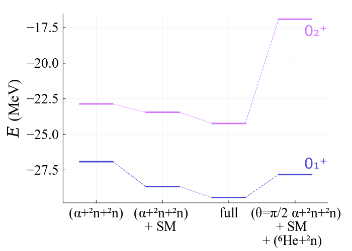
Figure 1: The energy spectra of ${}^{8}\mathrm{He}(0_{1}^{+})$ and ${}^{8}\mathrm{He}(0_{2}^{+})$ calculated with the truncated model spaces. The spectra obtained by using the $\alpha+{}^{2}n+{}^{2}n$ components, those using the $\alpha+{}^{2}n+{}^{2}n$ and the SM components, those of the full GCM calculation using the $\alpha+{}^{2}n+{}^{2}n$, SM, and $\mathrm{{}^{6}He}+{}^{2}n$ configurations are shown in the first, second, and third columns from the left. The result obtained with the $\theta$-fixed GCM calculation using $\alpha+{}^{2}n+{}^{2}n$ at $\theta=\pi/2$, SM, and $\mathrm{{}^{6}He}+{}^{2}n$ configurations are shown in the right column.

Also in ${}^{10}\mathrm{Be}$ system, the $2\alpha+{}^{2}n$ cluster component is dominant as 89% and 92% in ${}^{10}\mathrm{Be}(0_{1}^{+})$ and ${}^{10}\mathrm{Be}(0_{2}^{+})$, respectively. From these values, the dineutron cluster breaking component is estimated to be 11% and 8% in ${}^{10}\mathrm{Be}(0_{1}^{+})$ and ${}^{10}\mathrm{Be}(0_{2}^{+})$, respectively. For the ${}^{6}\mathrm{He}+\alpha$ cluster component, ${}^{10}\mathrm{Be}(0_{2}^{+})$ has an approximately 60% overlap with the ${}^{6}{\rm He}+\alpha$ cluster components, which indicates the spatial correlation between the dineutron cluster and an $\alpha$ cluster.

III.3 Effects of dineutron breaking in ${}^{8}\mathrm{He}$

Table 6: R.m.s. radii of the $0_{1}^{+}$ and $0_{2}^{+}$ states in ${}^{8}\mathrm{He}$, and the $0_{1}^{+}-0_{2}^{+}$ transition matrix elements $M$(IS0) obtained by the restricted GCM and the full GCM calculations

	$r_{m}(0_{1}^{+})$	$r_{m}(0_{2}^{+})$	$M$(IS0)
	(fm)	(fm)	($\mathrm{f}\mathrm{m}^{2}$)
$\alpha+{}^{2}n+{}^{2}n$	2.70	3.97	23.5
($\alpha+{}^{2}n+{}^{2}n$) + SM	2.40	3.86	16.3
full	2.40	3.91	15.5

In order to discuss the effects of the dineutron breaking components in ${}^{8}\mathrm{He}$, we perform restricted GCM calculations within truncated model spaces. We calculate ${}^{8}\mathrm{He}$ wave functions by superposing only $\alpha+{}^{2}n+{}^{2}n$ configurations ($\alpha+{}^{2}n+{}^{2}n$ calculation) but not ${}^{6}\rm{He}+{}^{2}n$ and SM configurations. We also perform calculations by using $\alpha+{}^{2}n+{}^{2}n$ and SM configurations ($(\alpha+{}^{2}n+{}^{2}n)$+SM calculation) but not $\mathrm{{}^{6}He}+{}^{2}n$ configurations.

The energy spectra obtained with the $\alpha+{}^{2}n+{}^{2}n$ calculation and the ($\alpha+{}^{2}n+{}^{2}n$)+SM calculation are compared with those of the full calculation in Figure 1 (three columns from the left). Comparing the results of the $\alpha+{}^{2}n+{}^{2}n$ and ($\alpha+{}^{2}n+{}^{2}n$)+SM calculations, one can see that the mixing of the SM configuration into the $\alpha+{}^{2}n+{}^{2}n$ configurations causes a significant energy gain as $1.7\text{\,}\mathrm{M}\mathrm{e}\mathrm{V}$ of the ground state, which is contributed by the spin-orbit interaction. This means that the dineutron breaking due to the spin-orbit interaction plays an essential role in the binding of the ${}^{8}\mathrm{He}$ system. It also contributes to a $0.78\text{\,}\mathrm{M}\mathrm{e}\mathrm{V}$ energy gain in the $0_{2}^{+}$ state, but it is not as large as the ground state because the effect of the spin-obit attraction is weaker for spatially developed dineutron clusters in ${}^{8}\mathrm{He}(0_{2}^{+})$.

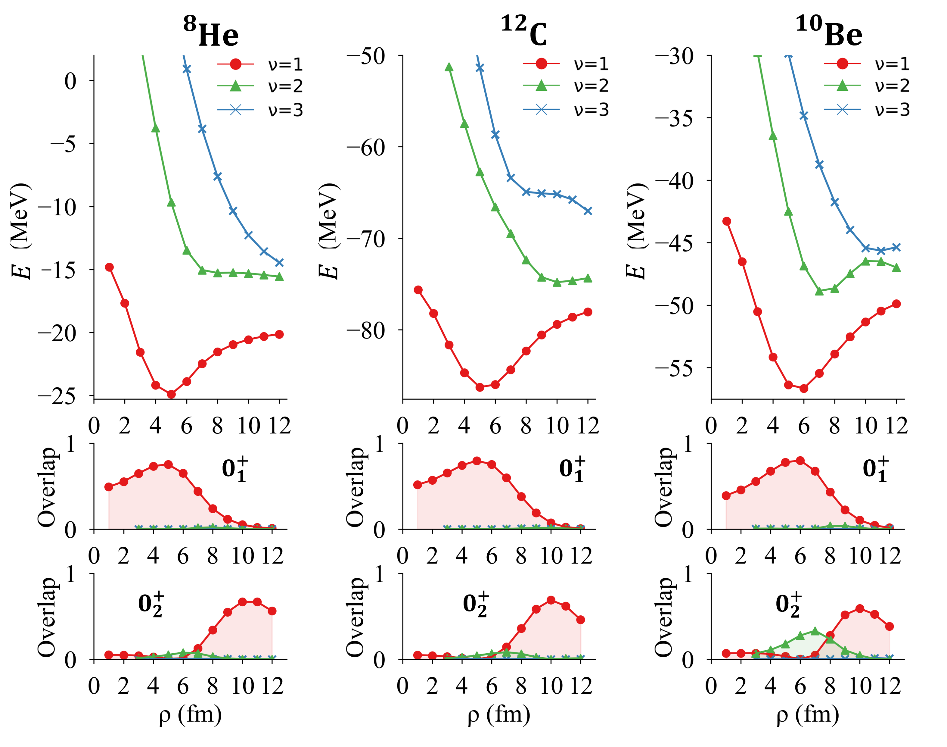
Figure 2: (Top) Energy spectra of ${}^{8}\mathrm{He},^{12}\mathrm{C}$ and ${}^{10}\mathrm{Be}$ of the $\rho$-fixed 3-body states plotted as functions of $\rho=\rho_{0}$. (Middle) Squared overlaps of the $\rho$-fixed states $\ket{\varphi_{\nu}(\rho_{0})}$ with the $0_{1}^{+}$ states. (Bottom) Those with the $0_{2}^{+}$ states. The results for $\nu=1$, $\nu=2$, and $\nu=3$ are shown by red circles, blue triangles, and green cross symbols, respectively.

In comparison of the ($\alpha+{}^{2}n+{}^{2}n$)+SM result with the full calculation, one can assess the effects of the $\mathrm{{}^{6}He}+{}^{2}n$ cluster component, in which two neutrons form a spatially developed dineutron but the other two neutrons stay in the $p_{3/2}$ orbit around the $\alpha$. The mixing of this $\mathrm{{}^{6}He}+{}^{2}n$ component generates an additional energy gain as $0.78\text{\,}\mathrm{M}\mathrm{e}\mathrm{V}$ for the $0_{1}^{+}$ and $0_{2}^{+}$ states.

The results of $r_{m}$ and $M$(IS0) obtained by the $\alpha+{}^{2}n+{}^{2}n$ calculation and those by the ($\alpha+{}^{2}n+{}^{2}n$)+SM calculation are listed in Table 6 together with those of the full calculation. Comparing the $\alpha+{}^{2}n+{}^{2}n$ results with the full calculation, it is found that the dineutron cluster breaking gives a significant contribution to the system size shrinking, in particular, of the ground state; an approximately 10% reduction in $r_{m}$, and a 30% reduction in $M$(IS0). These results indicate again that the spin-orbit interaction causes the deeper binding involving the dineutron cluster breaking as previously shown in the energy spectra in Figure 1.

Although the dineutron cluster breaking gives significant effects on the energies and nuclear size, but qualitative properties of ${}^{8}\mathrm{He}(0^{+}_{1})$ and ${}^{8}\mathrm{He}(0^{+}_{2})$ are similar between calculations with and without the dineutron cluster breaking. In other words, the $\alpha+{}^{2}n+{}^{2}n$ model can describe leading properties of ${}^{8}\mathrm{He}$, but combining it with the dineutron cluster breaking configurations is essential for a detailed description of ${}^{8}\mathrm{He}(0^{+}_{1})$ and ${}^{8}\mathrm{He}(0^{+}_{2})$ structures.

III.4 Radial behavior of 3-body cluster structures

In order to clarify the monopole excitation modes in ${}^{8}\mathrm{He}$, ${}^{10}\mathrm{Be}$, and ${}^{12}\mathrm{C}$, we prepare $\rho$-fixed 3-body states and take overlaps with the $0^{+}_{1}$ and $0^{+}_{2}$ states obtained by the full GCM calculations. The $\rho$-fixed 3-body states are constructed by the GCM calculation with the $\rho=\rho_{0}$ constraint as

$$\begin{split}&\ket{\varphi_{\nu}(\rho_{0})}\\ =&\int d\gamma\,d\theta\,f_{\nu}(\gamma,\theta)\hat{P}^{0+}\ket{C_{1},C_{2},C_{3};\rho=\rho_{0},\gamma,\theta},\end{split}$$ (29)

where the label $C_{1},C_{2},C_{3}$ are $\alpha+{}^{2}n+{}^{2}n$, $3\alpha$, and $2\alpha+{}^{2}n$ for ${}^{8}\mathrm{He}$, ${}^{12}\mathrm{C}$, and ${}^{10}\mathrm{Be}$, respectively, and $\nu=1,2$ is the label for the $\nu$th state in the $\rho$-fixed subspace. For each $\rho_{0}$ value, coefficients $f_{\nu}(\gamma,\theta)$ are determined by solving the Hill-Wheeler equation for the generator coordinates ($\gamma$ and $\theta$), and energy spectra $E_{\nu}(\rho_{0})$ are obtained. We also calculate the overlaps of these $\rho$-fixed states $\ket{\varphi_{\nu}(\rho_{0})}$ with the $0^{+}_{1}$ and $0^{+}_{2}$ states obtained by the full GCM calculations.

Figure 2 shows the $\rho$-fixed results of the energy spectra $E_{\nu}(\rho_{0})$ for $\nu=1,2,3$ and the squared overlaps of $\varphi_{\nu}(\rho_{0})$ with the full GCM wave functions plotted as functions of $\rho_{0}$. In all of ${}^{8}\mathrm{He}$, ${}^{12}\mathrm{C}$, and ${}^{10}\mathrm{Be}$, the ground states are almost exhausted by the $\nu=1$ states; they have the maximum overlap with the lowest state ($\nu=1$) at the energy minimum around $\rho=5$–$6\text{\,}\mathrm{f}\mathrm{m}$ and distribute along the $\nu=1$ energy curve.

The $0_{2}^{+}$ states of ${}^{8}\mathrm{He}$ and ${}^{12}\mathrm{C}$ are approximately exhausted by the $\nu=1$ states and have large overlaps around $\rho=$10\text{\,}\mathrm{f}\mathrm{m}$$. This means that the ${}^{8}\mathrm{He}(0_{2}^{+})$ and ${}^{12}\mathrm{C}(0^{+}_{2})$ are the radial excitation modes along $\rho$, and this is one of the similarities between ${}^{8}\mathrm{He}$ and ${}^{12}\mathrm{C}$. In contrast, ${}^{10}\mathrm{Be}(0_{2}^{+})$ is not simply described by the $\nu=1$ states but has significant overlaps with $\nu=2$ states around $\rho=$7\text{\,}\mathrm{f}\mathrm{m}$$. This is different from the cases of ${}^{8}\mathrm{He}(0_{2}^{+})$ and ${}^{12}\mathrm{C}(0^{+}_{2})$, and indicates an excitation from $\nu=1$ to $\nu=2$ states, rather than the radial excitation. The reason for this difference between ${}^{8}\mathrm{He}$, ${}^{12}\mathrm{C}$ and ${}^{10}\mathrm{Be}$ can be understood by the energy cost for the $\nu=1\to\nu=2$ excitation compared with the $\rho$ excitation along the $\nu=1$ states. The $\nu=2$ energy curve in ${}^{10}\mathrm{Be}$ shows an energy pocket around $\rho=$7\text{\,}\mathrm{f}\mathrm{m}$$, and its minimum energy approximately degenerates with the $\nu=1$ energy at $\rho=$12\text{\,}\mathrm{f}\mathrm{m}$$, meaning that the $\nu=2$ excitation occurs with the energy cost as small as the $\rho$ excitation and contributes to ${}^{10}\mathrm{Be}(0_{2}^{+})$. In the cases of ${}^{8}\mathrm{He}$ and ${}^{12}\mathrm{C}$, the $\nu=2$ energy curves do not show such a pocket and their energies are higher than the $\nu=1$ energy curve. As a result of the much energy costs for the $\nu=2$ states, ${}^{8}\mathrm{He}(0_{2}^{+})$ and ${}^{12}\mathrm{C}(0_{2}^{+})$ have the $\nu=1$ dominance feature without the $\nu=2$ mixing.

IV Discussions

IV.1 Detailed analyses of cluster structures in ${}^{8}\mathrm{He}$

IV.1.1 Spatial configurations of the $\alpha+{}^{2}n+{}^{2}n$ clusters in ${}^{8}\mathrm{He}(0_{2}^{+})$

As mentioned in the $\rho$-fixed analysis in the previous section, ${}^{8}\mathrm{He}(0_{2}^{+})$ is regarded as the radial excitation mode similar to ${}^{12}\mathrm{C}(0_{2}^{+})$. We here give further discussions on the spatial configurations of the $\alpha+{}^{2}n+{}^{2}n$ cluster component in ${}^{8}\mathrm{He}(0_{2}^{+})$. We calculate the squared overlap ${\cal O}^{\alpha+{}^{2}n+{}^{2}n}(\bm{d}_{1},\bm{d}_{2})$ of the $\alpha+{}^{2}n+{}^{2}n$ cluster configuration with ${}^{8}\mathrm{He}(0^{+}_{2})$ obtained by the full GCM calculation as,

$${\cal O}^{\alpha+{}^{2}n+{}^{2}n}(\bm{d}_{1},\bm{d}_{2})\equiv\left|\bra{\alpha+{}^{2}n+{}^{2}n;\bm{d}_{1},\bm{d}_{2}}\ket{{}^{8}\mathrm{He}(0_{2}^{+})}\right|^{2},$$ (30)

where $\bm{d}_{1}=\bm{R}_{1}-\bm{R}_{3}$ and $\bm{d}_{2}=\bm{R}_{2}-\bm{R}_{3}$ are coordinates of the two ${}^{2}n$ clusters measured from the $\alpha$ cluster. 3-body configurations in the $0^{+}$-projected states are specified by $d_{1}=|\bm{d}_{1}|$, $d_{2}=|\bm{d}_{2}|$, and the opening angle $\phi$ between $\bm{d}_{1}$ and $\bm{d}_{2}$, and therefore, we rewrite the overlap with the parameters $(d_{1},d_{2},\phi)$ instead of $(\bm{d}_{1},\bm{d}_{2})$ as ${\cal O}^{\alpha+{}^{2}n+{}^{2}n}(d_{1},d_{2},\phi)={\cal O}^{\alpha+{}^{2}n+{}^{2}n}(\bm{d}_{1},\bm{d}_{2})$. The results of the squared overlaps are shown in Figure 3. The calculated values of ${\cal O}^{\alpha+{}^{2}n+{}^{2}n}(d_{1},d_{2},\phi)$ for fixed $d_{1}$ values at $d_{1}=4,5$ and $6\text{\,}\mathrm{f}\mathrm{m}$ are plotted on the $(d_{2},\phi)$ plane in the top, middle, and bottom panels, respectively. These plots show spatial distributions of one dineutron when the center positions of the $\alpha$ cluster and the other dineutron are located at the origin (pink circles) and $\bm{d}_{1}=(d_{1},\phi=0)$ (lightblue circles), respectively.

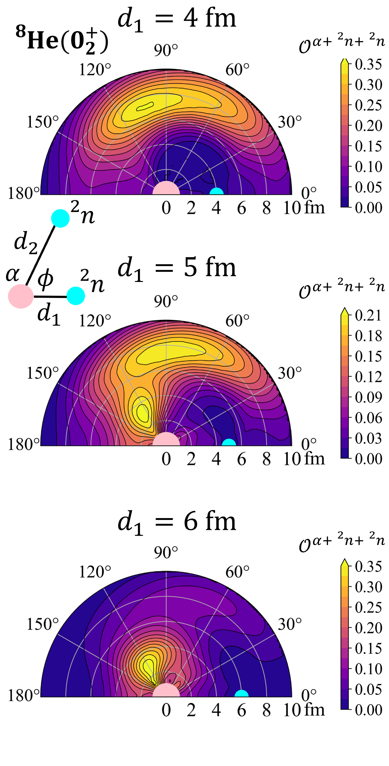
Figure 3: Spatial distribution of three clusters in ${}^{8}\mathrm{He}(0^{+}_{2})$. The squared overlap ${\cal O}^{\alpha+{}^{2}n+{}^{2}n}(d_{1},d_{2},\phi)$ for fixed $d_{1}$ values at $d_{1}=4$ fm (top), 5 fm (middle), and 6 fm (bottom) are plotted on the $(d_{2},\phi)$ plane. The center positions of the $\alpha$ cluster and the ${}^{2}n$ cluster are displayed at the origin (pink circles) and at $\bm{d}_{1}=(d_{1},\phi=0)$ (blue circles), respectively.

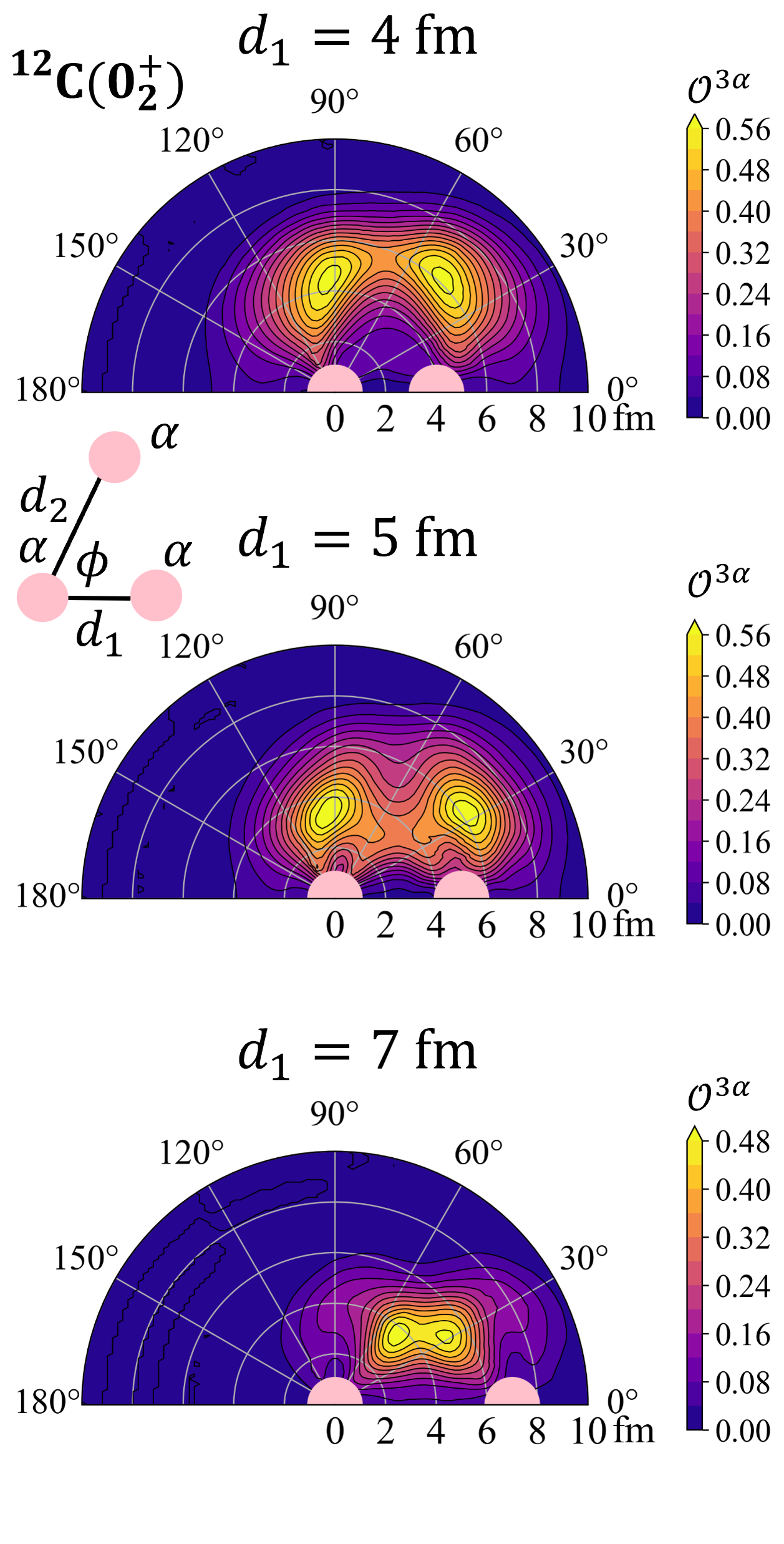
Figure 4: Same as Figure 3 but for $3\alpha$ clusters of in ${}^{12}\mathrm{C}(0_{2}^{+})$. ${\cal O}^{3\alpha}(d_{1},d_{2},\phi)$ for $d_{1}=4,5,7\,$\mathrm{f}\mathrm{m}$$ are shown in the top, middle, and bottom panels, respectively. Center positions of the fixed two $\alpha$ clusters are shown by pink circles.

In the $d_{1}=$4\text{\,}\mathrm{f}\mathrm{m}$$ case, the dineutron widely distributes along the angular direction around the $d_{2}=$7\text{\,}\mathrm{f}\mathrm{m}$$ region, which shows $S$-wave behavior of the two dineutrons around the $\alpha$ cluster. This $S$-wave feature is consistent with the results of the ${}^{2}n$-condensation model [14]. In the $d_{1}=$5\text{\,}\mathrm{f}\mathrm{m}$$ case, the $S$-wave $\alpha+{}^{2}n+{}^{2}n$ behavior still remains, but another peak appears around $d_{2}=$3\text{\,}\mathrm{f}\mathrm{m}$$, $\phi=120\textrm{--}$$$. This new peak exhibits 2-body-like $(\alpha+{}^{2}n)+{}^{2}n$ cluster structure, where one of two dineutrons approaches the $\alpha$ cluster and the other dineutron moves far from the $(\alpha+{}^{2}n)$ cluster, which consists of the correlated $\alpha$ and ${}^{2}n$ clusters. Note that this $\alpha+{}^{2}n$ correlation is induced by the attraction of the spin-orbit interaction via the ${}^{2}n$ cluster breaking. In $d_{1}=$6\text{\,}\mathrm{f}\mathrm{m}$$, there are no longer $S$-wave $\alpha+{}^{2}n+{}^{2}n$ structures but the 2-body-like $(\alpha+{}^{2}n)+{}^{2}n$ cluster structure is dominant.

From this analysis, ${}^{8}\mathrm{He}(0_{2}^{+})$ is characterized by two kinds of structures. One is the gas-like $\alpha+{}^{2}n+{}^{2}n$ structure of $S$-wave dineutrons, and the other is the 2-body-like $(\alpha+{}^{2}n)+{}^{2}n$ structure.

IV.1.2 $\theta$-fixed analysis

In order to discuss the role of the angle $\theta$ degree of freedom (DOF), we perform the $\theta$-fixed GCM calculation by fixing $\theta=\pi/2$ of $\alpha+{}^{2}n+{}^{2}n$ cluster configurations, which corresponds to isosceles triangular configurations with the $\alpha$ cluster at the vertex, as

$$\begin{split}&\ket{\theta\text{-}\mathrm{fixed}\,\,^{8}\mathrm{He}(0_{\nu}^{+})}\\ =&\int d\rho\,d\gamma\,f_{\nu}^{3B}(\rho,\gamma)\hat{P}^{0^{+}}\ket{\alpha+{}^{2}n+{}^{2}n;\rho,\gamma,\theta=\pi/2}\\ &+f_{\nu}^{SM}\ket{\Psi^{SM}}+\int da\,f_{\nu}^{2B}(a)\hat{P}^{0+}\ket{{}^{6}\mathrm{He}+{}^{2}n;a},\end{split}$$ (31)

where the coefficients $f_{\nu}^{3B}(\rho,\gamma),f_{\nu}^{SM},f_{\nu}^{2B}(a)$ are determined as explained in Sec. II.3. The energy spectra of the $\theta$-fixed calculation are shown in the right column of Figure 1. Comparing the energy spectra obtained by the $\theta=\pi/2$ fixing calculation with those of the full GCM calculation without $\theta$ fixing, one can see a significant energy gain, in particular, for the $0^{+}_{2}$ state. This result indicates that the angular DOF is important for the $\alpha+{}^{2}n+{}^{2}n$ cluster structure in the $0_{2}^{+}$ state and the superpositions of the $\alpha+{}^{2}n+{}^{2}n$ configurations along the angle $\theta$ is essential to describe the $S$-wave feature of the dineutron motion around the $\alpha$ in ${}^{8}\mathrm{He}(0^{+}_{2})$.

IV.1.3 Spatial development of the $\mathrm{{}^{6}He}+{}^{2}n$ cluster structure

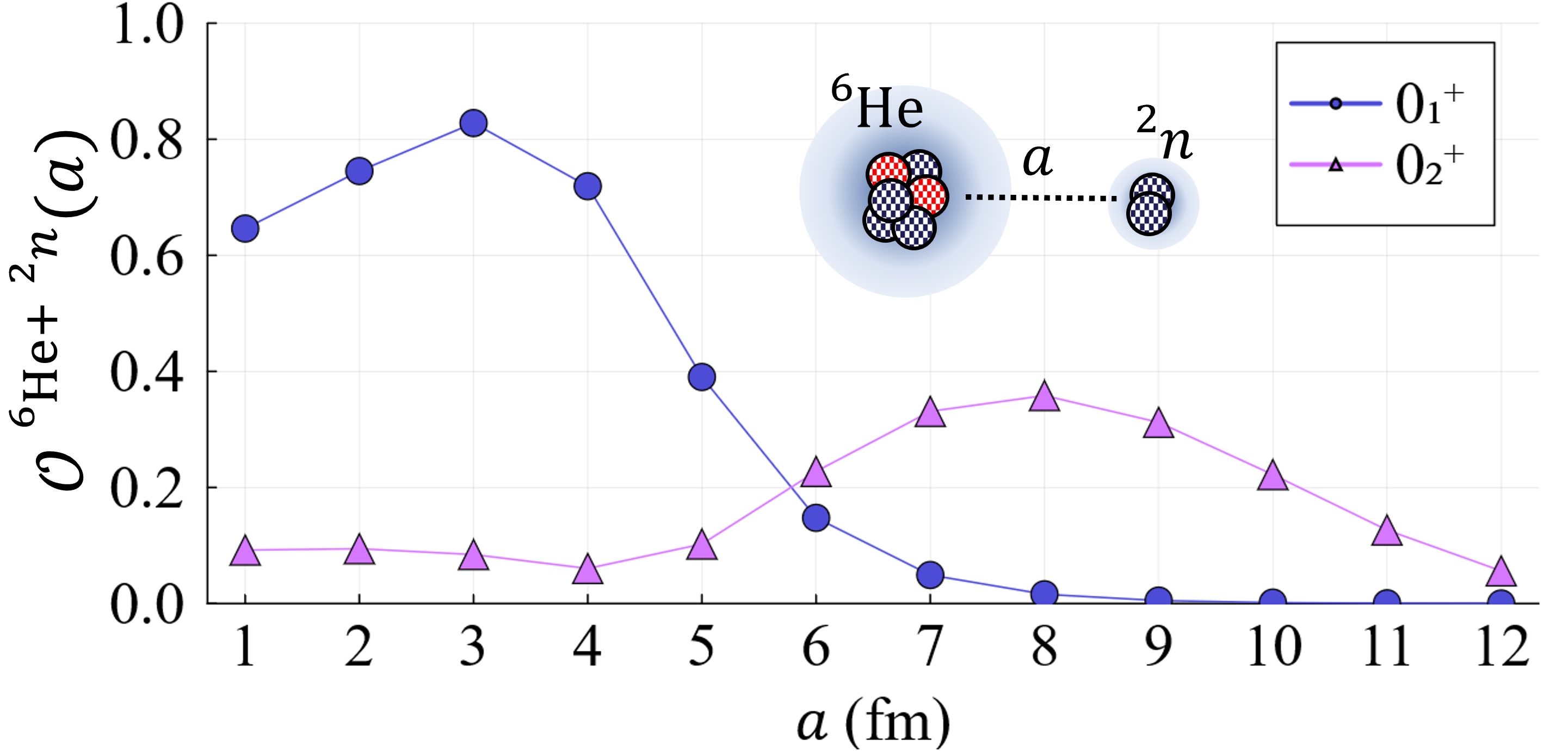
Figure 5: Squared overlaps ${\cal O}^{{}^{6}\textrm{He}+{}^{2}n}(a)$ with each ${}^{6}\mathrm{He}+{}^{2}n$ configuration at distance $a$ fm for ${}^{8}\mathrm{He}(0_{1}^{+})$ and ${}^{8}\mathrm{He}(0_{2}^{+})$. The results for ${}^{8}\mathrm{He}(0_{1}^{+})$ and ${}^{8}\mathrm{He}(0_{2}^{+})$ are plotted by blue circles and purple triangles, respectively.

As discussed previously in the 3-body analysis (Sec. IV.1.1), ${}^{8}\mathrm{He}(0_{2}^{+})$ contains the 2-body-like $(\alpha+{}^{2}n)+{}^{2}n$ component, which is induced by the attraction of the spin-orbit interaction via the ${}^{2}n$ cluster breaking. To discuss the spatial distribution of the ${}^{2}n$ cluster around the $\mathrm{{}^{6}He}$-cluster, we calculate the squared overlap ${\cal O}^{{}^{6}\textrm{He}+{}^{2}n}(a)$ of the ${}^{6}\mathrm{He}+{}^{2}n$ cluster configurations at the distance $a$ with the ${}^{8}\mathrm{He}(0^{+}_{1})$ and ${}^{8}\mathrm{He}(0^{+}_{2})$ wave functions obtained by the full GCM calculation as,

$$\begin{split}{\cal O}^{{}^{6}\textrm{He}+{}^{2}n}(a)\equiv\left|\bra{{}^{6}\mathrm{He}+{}^{2}n;a}\ket{{}^{8}\mathrm{He}(0_{1,2}^{+})}\right|^{2}.\end{split}$$ (32)

The calculated values of ${\cal O}^{{}^{6}\textrm{He}+{}^{2}n}(a)$ for the $0_{1}^{+}$ and $0_{2}^{+}$ states are shown in Figure 5. The $0_{1}^{+}$ state has large overlaps in the small distance region with a peak around $a=$3\text{\,}\mathrm{f}\mathrm{m}$$ and rapid damping in $a>$3\text{\,}\mathrm{f}\mathrm{m}$$, indicating the compact ${}^{6}\rm{He}+{}^{2}n$ cluster structures in the $0_{1}^{+}$ state. It should be noted that this compact ${}^{6}\rm{He}+{}^{2}n$ component has large overlaps with the SM and compact $\alpha+{}^{2}n+{}^{2}n$ cluster configurations. For the $0_{2}^{+}$ state, ${\cal O}^{{}^{6}\mathrm{He}+{}^{2}n}(a)$ shows a peak around $a=$8\text{\,}\mathrm{f}\mathrm{m}$$ and a long tail toward large $a$ regions. This result shows a weakly binding feature of the ${}^{6}\rm{He}+{}^{2}n$ cluster structure in ${}^{8}\mathrm{He}(0_{2}^{+})$, that is, a widely distributing dineutron around the ${}^{6}\rm{He}$-cluster. This is consistent with the 2-body-like structures $(\alpha+{}^{2}n)+{}^{2}n$ observed in the $\alpha+{}^{2}n+{}^{2}n$ analysis in Sec. IV.1.1.

IV.1.4 Spatial configurations of $3\alpha$ clusters in ${}^{12}\mathrm{C}(0^{+}_{2})$

We analyze the $3\alpha$ cluster structure in ${}^{12}\mathrm{C}$ and discuss analogies and differences of 3-body cluster structures between ${}^{12}\mathrm{C}(0_{2}^{+})$ and ${}^{8}\mathrm{He}(0_{2}^{+})$. As done for ${}^{8}\mathrm{He}$, we calculate the squared overlap of the $3\alpha$ cluster configurations ${\cal O}^{3\alpha}(d_{1},d_{2},\phi)$ as

$${\cal O}^{3\alpha}(d_{1},d_{2},\phi)={\cal O}^{3\alpha}(\bm{d}_{1},\bm{d}_{2})\equiv\left|\bra{{}^{12}\mathrm{C}(0_{2}^{+})}\ket{3\alpha;\bm{d}_{1},\bm{d}_{2}}\right|^{2}$$ (33)

with $\bm{d}_{1}=\bm{R}_{1}-\bm{R}_{3}$, $\bm{d}_{2}=\bm{R}_{2}-\bm{R}_{3}$, $d_{1}=|\bm{d}_{1}|$, $d_{2}=|\bm{d}_{2}|$ and $\phi$ is the opening angle between $\bm{d}_{1}$ and $\bm{d}_{2}$. The calculated values of ${\cal O}^{3\alpha}(d_{1},d_{2},\phi)$ for $d_{1}=4,5,$ and $7\text{\,}\mathrm{f}\mathrm{m}$ are shown in the top, middle, and bottom panels of Fig. 4, respectively. In the result of $d_{1}=$4\text{\,}\mathrm{f}\mathrm{m}$$, the $\alpha$ cluster widely distributes along $\phi$ direction, which suggests the $S$-wave nature of the $\alpha$ cluster motion in ${}^{12}\mathrm{C}(0^{+}_{2})$. This $S$-wave behavior is one of the similarities with the ${}^{8}\mathrm{He}(0_{2}^{+})$ structure. However, the spatial extent is weaker in ${}^{12}\mathrm{C}(0_{2}^{+})$ than in ${}^{8}\mathrm{He}(0_{2}^{+})$ as seen in the $d_{2}$ distribution in ${\cal O}^{3\alpha}(d_{1}=4~\textrm{fm},d_{2},\phi)$ compared with that in ${\cal O}^{\alpha+^{2}n+^{2}n}(d_{1}=4~\textrm{fm},d_{2},\phi)$; the former and the latter shows significant amplitudes in the $d_{2}=4\textrm{--}6$ fm regions and $d_{2}=6$–$10$ fm regions, respectively. In other words, the weakly binding 3-body feature of the $\alpha+{}^{2}n+{}^{2}n$ cluster structure in ${}^{8}\mathrm{He}(0^{+}_{2})$ is enhanced compared with that of the $3\alpha$ cluster structure in ${}^{12}\mathrm{C}(0^{+}_{2})$. This feature can also be seen in the larger $r_{m}$ of ${}^{8}\mathrm{He}(0_{2}^{+})$ than that of ${}^{12}\mathrm{C}(0_{2}^{+})$. Another difference from ${}^{8}\mathrm{He}(0^{+}_{2})$ is that the 2-body-like $(\alpha+\alpha)+\alpha$ structure does not appear in ${}^{12}\mathrm{C}(0_{2}^{+})$. As seen in the result of $d_{1}=$7\text{\,}\mathrm{f}\mathrm{m}$$, the amplitude concentrates at $d_{2}\sim$4\text{\,}\mathrm{f}\mathrm{m}$$ and $\phi\sim$$$, which corresponds to a collapsed isosceles triangle configuration of $3\alpha$ clusters instead of the 2-body-like structure. This feature can be understood by the difference in the inter-cluster interactions between the $\alpha+\alpha$ and $\alpha+^{2}n$ systems. Namely, the $\alpha+\alpha$ correlation is unfavored because of the nucleon Pauli blocking effect, and the absence of the spin-orbit attraction at short distances.

V summary

We investigated the structures of the $0_{1}^{+}$ and $0_{2}^{+}$ states of ${}^{8}\mathrm{He}$ with a microscopic cluster model combined with the cluster breaking configurations, and analyzed the $\alpha+{}^{2}n+{}^{2}n$ cluster structures and the dineutron breaking effects induced by the spin-orbit interaction. For describing dineutron motions in detail, we superposed the $\alpha+{}^{2}n+{}^{2}n$ cluster and ${}^{6}\rm{He}+{}^{2}n$ cluster configurations in the GCM framework, and also incorporated the mixing of the shell-model (SM) configuration.

We calculated the energies and r.m.s. radii of the $0_{1,2}^{+}$ states and the matrix element of the $0_{1}^{+}-0_{2}^{+}$ transition $M$(IS0), and found that the calculated results are in reasonable agreement with the experimental values and other theoretical calculations. In the results, we obtained a compact structure of the $0_{1}^{+}$ state, and the developed $\alpha+{}^{2}n+{}^{2}n$ cluster structure in the $0_{2}^{+}$ state.

The $\alpha+{}^{2}n+{}^{2}n$ cluster component has dominant contributions in both ${}^{8}\mathrm{He}(0_{1}^{+})$ and ${}^{8}\mathrm{He}(0_{2}^{+})$. The $0_{1}^{+}$ state is a mixture of the compact $\alpha+{}^{2}n+{}^{2}n$ cluster structures and the SM component, while the $0_{2}^{+}$ state has the spatially developed $\alpha+{}^{2}n+{}^{2}n$ structures and also the ${}^{6}\rm{He}+{}^{2}n$ structures, showing the spatial correlation between the $\alpha$ and ${}^{2}n$ cluster in the 3-body cluster dynamics.

In comparison of the results obtained with and without the ${}^{2}n$ cluster breaking, it was revealed that the dineutron cluster breaking gives important contributions to the energy gain and size shrinking of the $0_{1}^{+}$ and $0_{2}^{+}$ states.

We also calculated the $0_{1}^{+}$ and $0_{2}^{+}$ states of ${}^{12}\mathrm{C}$ and ${}^{10}\mathrm{Be}$ by respectively applying the $3\alpha$ and $2\alpha+{}^{2}n$ cluster models combined with cluster breaking configurations, and compared the properties of the monopole excitations with those of ${}^{8}\mathrm{He}$. It was found that the excitation to the $0_{2}^{+}$ states in ${}^{8}\mathrm{He}$ and ${}^{12}\mathrm{C}$ are regarded as the radial excitation modes along the hyperradius $\rho$, whereas the $0_{2}^{+}$ state in ${}^{10}\mathrm{Be}$ is not described by the radial excitation but shows different characters from those in ${}^{8}\mathrm{He}$ and ${}^{12}\mathrm{C}$.

References

- Matsuo [2006] M. Matsuo, Phys. Rev. C 73, 044309 (2006).
- Catara et al. [1984] F. Catara, A. Insolia, E. Maglione, and A. Vitturi, Phys. Rev. C 29, 1091 (1984).
- Pillet et al. [2007] N. Pillet, N. Sandulescu, and P. Schuck, Phys. Rev. C 76, 024310 (2007).
- Esbensen and Bertsch [1992] H. Esbensen and G. Bertsch, Nucl. Phys. A 542, 310 (1992).
- Oganessian et al. [1999] Y. T. Oganessian, V. I. Zagrebaev, and J. S. Vaagen, Phys. Rev. Lett. 82, 4996 (1999).
- Hagino and Sagawa [2005] K. Hagino and H. Sagawa, Phys. Rev. C 72, 044321 (2005).
- Nakamura et al. [2006] Nakamura et al., Phys. Rev. Lett. 96, 252502 (2006).
- Duer et al. [2022] M. Duer et al., Nature 606, 678 (2022).
- Hiyama et al. [2016] E. Hiyama, R. Lazauskas, J. Carbonell, and M. Kamimura, Phys. Rev. C 93, 044004 (2016).
- Lazauskas et al. [2023] R. Lazauskas, E. Hiyama, and J. Carbonell, Phys. Rev. Lett. 130, 102501 (2023).
- Hagino et al. [2008] K. Hagino, N. Takahashi, and H. Sagawa, Phys. Rev. C 77, 054317 (2008).
- Yamaguchi et al. [2023] Y. Yamaguchi, W. Horiuchi, T. Ichikawa, and N. Itagaki, Phys. Rev. C 108, L011304 (2023).
- Kanada-En’yo [2007a] Y. Kanada-En’yo, Phys. Rev. C 76, 044323 (2007a).
- Kobayashi and Kanada-En’yo [2013] F. Kobayashi and Y. Kanada-En’yo, Phys. Rev. C 88, 034321 (2013).
- Myo et al. [2010] T. Myo, R. Ando, and K. Katō, Phys. Lett. B 691, 150 (2010).
- Yang et al. [2023] Z. H. Yang et al., Phys. Rev. Lett. 131, 242501 (2023).
- Yamada et al. [2008] T. Yamada, Y. Funaki, H. Horiuchi, K. Ikeda, and A. Tohsaki, Prog. of Theor. Phys. 120, 1139 (2008).
- Hill and Wheeler [1953] D. L. Hill and J. A. Wheeler, Phys. Rev. 89, 1102 (1953).
- Griffin and Wheeler [1957] J. J. Griffin and J. A. Wheeler, Phys. Rev. 108, 311 (1957).
- Itagaki et al. [2005] N. Itagaki, H. Masui, M. Ito, and S. Aoyama, Phys. Rev. C 71, 064307 (2005).
- Suhara et al. [2013] T. Suhara, N. Itagaki, J. Cseh, and M. Płoszajczak, Phys. Rev. C 87, 054334 (2013).
- Suhara and Kanada-En’yo [2015] T. Suhara and Y. Kanada-En’yo, Phys. Rev. C 91, 024315 (2015).
- Brink [1965] D. M. Brink, International school of physics “enrico fermi,” course xxxvi, varenna (1965).
- Kanada-En’yo and Horiuchi [1995] Y. Kanada-En’yo and H. Horiuchi, Prog. Theor. Phys. 93, 115 (1995).
- Kanada-En’yo et al. [2012] Y. Kanada-En’yo, M. Kimura, and A. Ono, Prog. Theor. Exp. Phys. 2012 (2012).
- Suhara and Kanada-En’yo [2010] T. Suhara and Y. Kanada-En’yo, Prog. Theor. Phys. 123, 303 (2010).
- Kanada-En’yo [2016] Y. Kanada-En’yo, Phys. Rev. C 94, 024326 (2016).
- Descouvemont [2019] P. Descouvemont, Phys. Rev. C 99, 064308 (2019).
- Suno et al. [2015] H. Suno, Y. Suzuki, and P. Descouvemont, Phys. Rev. C 91, 014004 (2015).
- Korennov and Descouvemont [2004] S. Korennov and P. Descouvemont, Nucl. Phys. A 740, 249 (2004).
- Volkov [1965] A. Volkov, Nucl. Phys. 74, 33 (1965).
- Aoyama et al. [2006] S. Aoyama, N. Itagaki, and M. Oi, Phys. Rev. C 74, 017307 (2006).
- Tilley et al. [2004] D. Tilley, J. Kelley, J. Godwin, D. Millener, J. Purcell, C. Sheu, and H. Weller, Nucl. Phys. A 745, 155 (2004).
- Alkhazov et al. [1997] G. D. Alkhazov et al., Phys. Rev. Lett. 78, 2313 (1997).
- Tanihata et al. [1992] I. Tanihata, D. Hirata, T. Kobayashi, S. Shimoura, K. Sugimoto, and H. Toki, Phys. Lett. B 289, 261 (1992).
- Mueller et al. [2007] P. Mueller, I. A. Sulai, A. C. C. Villari, J. A. Alcántara-Núñez, R. Alves-Condé, K. Bailey, G. W. F. Drake, M. Dubois, C. Eléon, G. Gaubert, R. J. Holt, R. V. F. Janssens, N. Lecesne, Z.-T. Lu, T. P. O’Connor, M.-G. Saint-Laurent, J.-C. Thomas, and L.-B. Wang, Phys. Rev. Lett. 99, 252501 (2007).
- Navas et al. [2024] S. Navas et al. (Particle Data Group Collaboration), Phys. Rev. D 110, 030001 (2024).
- Yamaguchi et al. [1979] N. Yamaguchi, T. Kasahara, S. Nagata, and Y. Akaishi, Prog. Theor. Phys. 62, 1018 (1979).
- Tamagaki [1968] R. Tamagaki, Prog. Theor. Phys. 39, 91 (1968).
- Kelley et al. [2017] J. Kelley, J. Purcell, and C. Sheu, Nucl. Phys. A 968, 71 (2017).
- Ozawa et al. [2001] A. Ozawa, T. Suzuki, and I. Tanihata, Nucl. Phys. A 693, 32 (2001).
- Chernykh et al. [2010] M. Chernykh, H. Feldmeier, T. Neff, P. v. Neumann-Cosel, and A. Richter, Phys. Rev. Lett. 105, 022501 (2010).
- Tohsaki et al. [2001] A. Tohsaki et al., Phys. Rev. Lett. 87, 192501 (2001).
- Funaki et al. [2003] Y. Funaki, A. Tohsaki, H. Horiuchi, P. Schuck, and G. Röpke, Phys. Rev. C 67, 051306 (2003).
- Kanada-En’yo [2007b] Y. Kanada-En’yo, Prog. Theor. Phys. 117, 655 (2007b).
- Tanihata et al. [1985] I. Tanihata, H. Hamagaki, O. Hashimoto, Y. Shida, N. Yoshikawa, K. Sugimoto, O. Yamakawa, T. Kobayashi, and N. Takahashi, Phys. Rev. Lett. 55, 2676 (1985).
- Nörtershäuser et al. [2009] W. Nörtershäuser, D. Tiedemann, M. Žáková, Z. Andjelkovic, K. Blaum, M. L. Bissell, R. Cazan, G. W. F. Drake, C. Geppert, M. Kowalska, J. Krämer, A. Krieger, R. Neugart, R. Sánchez, F. Schmidt-Kaler, Z.-C. Yan, D. T. Yordanov, and C. Zimmermann, Phys. Rev. Lett. 102 (2009).
- Itagaki and Okabe [2000] N. Itagaki and S. Okabe, Phys. Rev. C 61, 044306 (2000).
- Itagaki et al. [2000] N. Itagaki, S. Okabe, and K. Ikeda, Phys. Rev. C 62, 034301 (2000).
- Kanada-En’yo and Suhara [2012] Y. Kanada-En’yo and T. Suhara, Phys. Rev. C 85, 024303 (2012).