Equivariant Eikonal Neural Networks:
Grid-Free, Scalable Travel-Time Prediction on Homogeneous Spaces

Abstract

We introduce Equivariant Neural Eikonal Solvers, a novel framework that integrates Equivariant Neural Fields (ENFs) with Neural Eikonal Solvers. Our approach employs a single neural field where a unified shared backbone is conditioned on signal-specific latent variables – represented as point clouds in a Lie group – to model diverse Eikonal solutions. The ENF integration ensures equivariant mapping from these latent representations to the solution field, delivering three key benefits: enhanced representation efficiency through weight-sharing, robust geometric grounding, and solution steerability. This steerability allows transformations applied to the latent point cloud to induce predictable, geometrically meaningful modifications in the resulting Eikonal solution. By coupling these steerable representations with Physics-Informed Neural Networks (PINNs), our framework accurately models Eikonal travel-time solutions while generalizing to arbitrary Riemannian manifolds with regular group actions. This includes homogeneous spaces such as Euclidean, position–orientation, spherical, and hyperbolic manifolds. We validate our approach through applications in seismic travel-time modeling of 2D and 3D benchmark datasets. Experimental results demonstrate superior performance, scalability, adaptability, and user controllability compared to existing Neural Operator-based Eikonal solver methods.

1 Introduction

The eikonal equation is a first-order nonlinear partial differential equation (PDE) that plays a central role in a wide range of scientific and engineering applications. Serving as the high-frequency approximation to the wave equation (Noack and Clark, 2017), its solution represents the shortest arrival time from a source point to any receiver point within a specified scalar velocity field (Sethian, 1996). This formulation underpins numerous applications: in Computer Vision, it is integral to the computation of Signed Distance Functions (SDFs) (Jones et al., 2006) and geodesic-based image segmentation (Chen and Cohen, 2019); in Robotics, it facilitates optimal motion planning and inverse kinematics (Ni and Qureshi, 2023; Li et al., 2024b); and in Geophysics, it models seismic wave propagation through heterogeneous media, enabling critical travel-time estimations (Abgrall and Benamou, 1999; Rawlinson et al., 2010; Schuster and Quintus-Bosz, 1993).

Conventional numerical solvers, such as the Fast Marching Method (FMM) (Sethian, 1996) and the Fast Sweeping Method (FSM) (Zhao, 2004), have historically been used to compute solutions to the eikonal equation. However, these approaches are heavily dependent on spatial discretization, leading to a challenging trade-off: higher resolution is required for complex velocity models, which in turn dramatically increases computational and memory demands (Grubas et al., 2023; Song et al., 2024; Mei et al., 2024; Smith et al., 2021; Waheed et al., 2021). This issue is exacerbated in scenarios involving complex input geometries, such as Riemannian manifolds, which are prevalent in both computer vision (Bekkers et al., 2015) and robotics applications (Li et al., 2024b).

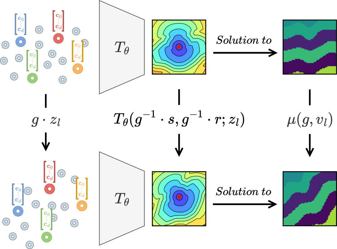
Figure 1: Steerability in the Equivariant Neural Eikonal Solver (E-NES) enables weight sharing across the entire group orbit: applying a group transformation to the conditioning variable $z_{l}$, induces a corresponding transformation on the travel-time function $T_{\theta}(\cdot,\cdot;z_{l})$ through the group’s left regular representation, and on the associated velocity field $v_{l}$ via the non-linear group action $\mu$, as formalized in Section 4.1.

Recent advances in scientific machine learning have introduced neural network-based solvers as promising alternatives. Physics-Informed Neural Networks (PINNs) integrate the PDE constraints into the training loss, offering a grid-free approximation to the eikonal equation and alleviating the discretization issues inherent in traditional numerical methods (Smith et al., 2021; Waheed et al., 2021; Ni and Qureshi, 2023; Grubas et al., 2023; Li et al., 2024b). However, a significant limitation of PINN-like approaches is their requirement to train a new network for each distinct velocity field, which hampers their applicability in real-time scenarios.

Neural Operators overcome this constraint by learning mappings between function spaces – specifically, from velocity fields to their corresponding travel-time solutions. Unlike PINNs, neural operators utilize a shared backbone and incorporate conditioning variables to handle different velocity profiles (Song et al., 2024; Mei et al., 2024). Current approaches leveraging simple architectures such as DeepONet (Mei et al., 2024) and Fourier Neural Operators (Song et al., 2024) have demonstrated promising results, yet there remain several avenues for improvement, as discussed in Section 2.

As stated in Wang et al. (2024b), one promising direction is to recognize that Neural Operators belong to a broader class of models known as Conditional Neural Fields. These models, which have been popularized within the Computer Vision community, explore advanced conditioning techniques to enhance expressivity, adaptability, and controllability (Dupont et al., 2022; Wessels et al., 2024; Wang et al., 2024b). In this work, we focus on the recently introduced Equivariant Neural Fields, which ground these conditioning variables in geometric principles, leading to improved representation quality and steerability – ensuring that transformations in the latent space correspond directly to transformations in the solution space (Knigge et al., 2024).

Our key contributions are as follows:

• We introduce a novel, expressive generalization of Equivariant Neural Fields to functions defined over products of Riemannian manifolds with regular group actions, including homogeneous spaces associated with linear Lie groups.

• We implement this framework through our Equivariant Neural Eikonal Solver (E-NES), to efficiently solve eikonal equations by leveraging geometric symmetries, enabling generalization across group transformations without explicit data augmentation (see Figure 1).

• We validate our approach through comprehensive experiments on 2D and 3D seismic travel-time benchmarks, achieving superior scalability, adaptability, and user controllability compared to existing methods in a grid-free manner.

2 Related work

Neural eikonal solvers.

Initial neural approaches for solving the eikonal equation have primarily relied on Physics-Informed Neural Networks (PINNs), which incorporate the PDE directly into the loss function (Smith et al., 2021; Waheed et al., 2021; Ni and Qureshi, 2023; Grubas et al., 2023; Li et al., 2024b; Kelshaw and Magri, 2024). These models are trained individually for each velocity field, achieving high-accuracy reconstructions at the expense of significant computational and memory overhead. Moreover, this per-instance training lacks cross-instance generalization, limiting its practicality for large-scale or real-time applications.

To enable generalization across velocity fields, operator learning methods have been proposed. DeepONet variants (Lu et al., 2021; Mei et al., 2024) learn mappings between function spaces, but typically require discretization of either the source or receiver points. This limits resolution invariance and complicates applications requiring continuous evaluations, such as geodesic path planning. Moreover, some methods such as Mei et al. (2024), rely on the supervision of a numerical solver, which can be beneficial in some simple scenarios but a bottleneck on complex ones.

Current Fourier Neural Operator approaches (Song et al., 2024) offer solver-free alternatives and incorporate the PDE into the loss, but still rely on partial discretization, inheriting similar resolution constraints.

In contrast, our method avoids discretization entirely by representing both inputs continuously and training solely with PDE supervision. We adopt the Conditional Neural Field (CNF) framework as our backbone, enabling scalable conditioning on velocity fields while preserving grid-free inference and resolution independence.

From Conditional to Equivariant Neural Fields.

Conditional Neural Fields (CNFs) constitute a class of coordinate-based neural networks trained to reconstruct continuous signals from discrete samples. Formally, a CNF is defined as $f_{\theta}:\mathcal{M}\times\mathcal{Z}\to\mathbb{R}^{d}$, parameterized by weights $\theta$, which maps a coordinate $p\in\mathcal{M}$ and a conditioning latent $z\in\mathcal{Z}$ to a $d$-dimensional output $f_{\theta}(p;z)$ approximating the target signal $f(p)$. Given a dataset $\mathcal{D}=\{f_{i}\}_{i=1}^{n}$ of continuous signals $f_{i}:\mathcal{M}\to\mathbb{R}^{d}$, each signal $f_{l}$ can be associated with a latent code $z_{l}$ such that a single network $f_{\theta}$ can represent the entire dataset: $f_{\theta}(p;z_{l})\approx f_{l}(p)$, for all $f_{l}\in\mathcal{D}$.

Dupont et al. (2022) first introduced a global latent vector for conditioning CNFs. Later works demonstrated that conditioning via a learnable point cloud $\{z_{i}\}_{i=1}^{m}\subseteq\mathcal{Z}$ enhances expressivity and reconstruction fidelity (Bauer et al., 2023; Luijmes et al., 2025; Kazerouni et al., 2025; Wessels et al., 2024). Equivariant Neural Fields further embed symmetry priors by enforcing the steerability property under a group $G$: $f_{\theta}(g^{-1}\cdot p;\{z_{i}\}_{i=1}^{m})=f_{\theta}(p;\{g\cdot z_{i}\}_{i=1}^{m}),$ for all $g\in G$. This equivariant formulation improves generalization and sample efficiency (Wessels et al., 2024; Chen et al., 2022; Chatzipantazis et al., 2023), and transfers left-actions on functions on the input space to clear direct left-actions in the latent space. In this work, we extend the point-cloud architecture of Wessels et al. (2024) to incorporate equivariance, yielding more expressive and symmetry-aware eikonal equation solvers.

Learning invariant functions.

As demonstrated in Wessels et al. (2024); Chen et al. (2022); Chatzipantazis et al. (2023), the steerability of Equivariant Neural Fields can be achieved if and only if the function is invariant with respect to transformations of both input and latent variables. Formally, this requires $f(g\cdot p;\{g\cdot z_{i}\}_{i=1}^{m})=f(p;\{z_{i}\}_{i=1}^{m})$ for all group elements $g$. Consequently, learning expressive invariant functions becomes a key requirement for our method.

A standard strategy from Invariant Theory is to identify a complete set of fundamental invariants. These fundamental invariants possess two critical properties: (1) any other invariant can be expressed as a function of these basic elements, and (2) they separate orbits—meaning that two points $p,q\in\mathcal{M}$ lie in the same orbit if and only if $I_{\upsilon}(p)=I_{\upsilon}(q)$ for all invariants $I_{\upsilon}:\mathcal{M}\to\mathbb{R}$ in the set (Olver, 1995). Several approaches have been developed for computing these invariants, including using Weyl’s First Main Theorem (Weyl, 1946; Villar et al., 2021), infinitesimal Lie algebra methods (Andreassen, 2020), moving frames (Olver, 2001), differential invariants (Olver, 1995; Sangalli et al., 2022; Li et al., 2024a), and other efficient separating invariant computations (Blum-Smith et al., 2024; Dym and Gortler, 2023). In our work, we leverage the moving frame technique from Olver (2001) due to its simplicity and its natural connection to modern invariant representation learning approaches, such as canonicalization (Shumaylov et al., 2024). A more detailed comparison with canonicalization methods is provided in the Appendix (Section B).

Moreover, rather than relying on global canonicalization—which produces a single canonical representation for an entire point cloud—we adopt a local canonicalization strategy (Hu et al., 2024; Wessels et al., 2024; Chen et al., 2022; Du et al., 2022; Wang et al., 2024a; Zhang et al., 2019). By canonicalizing small patches, our approach is better able to capture relevant local information and facilitates the use of transformer-based architectures, as opposed to the DeepSet-based architectures commonly employed in Blum-Smith et al. (2024); Dym and Gortler (2023); Villar et al. (2021).

3 Background

In this section, we present the necessary mathematical foundations and formulate the eikonal equation problem. For a comprehensive treatment of these topics, we refer the reader to Lee (2018); Olver (1995).

3.1 Mathematical Preliminaries

Differential Geometry.

A Riemannian manifold is defined as a pair $(\mathcal{M},\mathcal{G})$, where $\mathcal{M}$ is a smooth manifold and $\mathcal{G}$ is a Riemannian metric tensor field on $\mathcal{M}$ (Lee, 2018). The metric tensor $\mathcal{G}_{p}:T_{p}\mathcal{M}\times T_{p}\mathcal{M}\to\mathbb{R}$ assigns to each $p\in\mathcal{M}$ a positive-definite inner product on the tangent space $T_{p}\mathcal{M}$. Specifically, for any tangent vectors $\dot{p}_{1},\dot{p}_{2}\in T_{p}\mathcal{M}$, the inner product is given by $\mathcal{G}_{p}(\dot{p}_{1},\dot{p}_{2})$, and the corresponding norm is defined as $\left\lVert\dot{p}_{1}\right\rVert_{\mathcal{G}}=\sqrt{\mathcal{G}_{p}(\dot{p}_{1},\dot{p}_{1})}.$

The Riemannian distance between two points $p$ and $q$ in a connected manifold $\mathcal{M}$, denoted as $d_{\mathcal{G}}(p,q)$, is defined as the infimum of the length of all smooth curves joining them (Lee, 2018). Curves that achieve this infimum while traveling at constant speed are known as geodesics.

For a smooth scalar field $f:\mathcal{M}\to\mathbb{R}$, the Riemannian gradient $\operatorname{grad}f$ is the unique vector field reciprocal to the differential $\mathop{}\!\mathrm{d}f:T\mathcal{M}\to\mathbb{R}$, meaning $\mathcal{G}(\operatorname{grad}f,\,\cdot\,)=\mathop{}\!\mathrm{d}f$. Given a smooth function $\phi:\mathcal{M}\to\mathcal{M}$, we can also define the adjoint of a differential $\mathop{}\!\mathrm{d}\phi(p):T_{p}\mathcal{M}\to T_{\phi(p)}\mathcal{M}$ at a point $p\in\mathcal{M}$ as the map $(\mathop{}\!\mathrm{d}\phi(p))^{*}:T_{\phi(p)}\mathcal{M}\to T_{p}\mathcal{M};$ such that for every $\dot{p}\in T_{p}\mathcal{M},\dot{q}\in T_{\phi(p)}\mathcal{M}$ we have that $\mathcal{G}_{\phi(p)}(\mathop{}\!\mathrm{d}\phi(p)[\dot{p}],\dot{q})=\mathcal{G}_{p}(\dot{p},(\mathop{}\!\mathrm{d}\phi(p))^{*}[\dot{q}])$ (Lezcano-Casado, 2019).

Note that when $\mathcal{M}=\mathbb{R}^{n}$ and $\mathcal{G}_{p}=\mathbf{I}_{n}$ for all $p\in\mathbb{R}^{n}$, all Riemannian notions reduce to their Euclidean counterparts.

Group Theory.

A Lie group $G$ is a smooth manifold with group operations that are smooth. A (left) group action on a set $X$ is a map $\mu:G\times X\to X$ satisfying $\mu(e,x)=x$ and $\mu(g,\mu(h,x))=\mu(gh,x)$ for all $x\in X$, $g,h\in G$. When $\mu$ is clear by the context we write $g\cdot x$. The orbit space $X/G$ is the quotient space obtained by identifying points in $X$ that lie in the same orbit under the $G$-action. Formally, $X/G=\{\text{Orb}(x)\mid x\in X\}$ consists of all distinct orbits, where each orbit $\text{Orb}(x)=\{g\cdot x\mid g\in G\}$ represents an equivalence class under the relation $x\sim y\Leftrightarrow\exists g\in G\text{ such that }y=g\cdot x$. These equivalence classes partition $X$ into mutually disjoint subsets whose union equals $X$, yielding a canonical decomposition that reflects the underlying symmetry of the group action.

In this work, we will focus on the Special Euclidean group $SE(n)=\mathbb{R}^{n}\rtimes SO(n)$, representing roto-translations. For $g=(\mathbf{t},R)\in SE(n)$, the group product is $g\cdot g^{\prime}=(\mathbf{t},R)(\mathbf{t}^{\prime},R^{\prime})=(\mathbf{t}+R\mathbf{t}^{\prime},\,RR^{\prime})$.

The isotropy subgroup (or stabilizer) at $x\in X$ is $G_{x}=\{g\in G\mid g\cdot x=x\}$. A group $G$ acts freely if $G_{x}=\{e\}$ for all $x\in X$, meaning no non-identity element fixes any point. An $r$-dimensional Lie group acts freely on a manifold $\mathcal{M}$ if and only if its orbits have dimension $r$ (Olver, 1995). A group acts regularly on $\mathcal{M}$ if each point has arbitrarily small neighborhoods whose intersections with each orbit are connected. In practical applications, the groups of interest typically act regularly.

As discussed in Section 2, it is crucial for building Equivariant Neural Fields to obtain a complete set of functionally independent invariants. As demonstrated by Olver (2001), when a Lie group acts freely and regularly, such a set can be systematically derived locally using the moving frame method – detailed in the Appendix (Section B).

3.2 Eikonal Equation Formulation

On a Riemannian manifold $(\mathcal{M},\mathcal{G})$, the two-point Riemannian Eikonal equation with respect to a velocity field $v:\mathcal{M}\rightarrow[v_{\min},v_{\max}]$ (where $0<v_{\min}\leq v_{\max}<\infty$) is:

$$\begin{cases}\|\operatorname{grad}_{s}T(s,r)\|_{\mathcal{G}}=v(s)^{-1},\\ \|\operatorname{grad}_{r}T(s,r)\|_{\mathcal{G}}=v(r)^{-1},\\ T(s,r)=T(r,s),\quad T(s,s)=0,\end{cases}$$ (1)

where $\operatorname{grad}_{s}$ and $\operatorname{grad}_{r}$ denote the Riemannian gradients with respect to the source $s\in\mathcal{M}$ and the receiver $r\in\mathcal{M}$, respectively. The solution $T\colon\mathcal{M}\times\mathcal{M}\to\mathbb{R}_{+}$ corresponds to the travel-time function, and the interval $[v_{\min},v_{\max}]$ specifies the minimum and maximum velocity values in the training set.

To avoid irregular behavior as $r\to s$, it is common practice to factorize the travel-time function as

$$T(s,r)=\tilde{d}(s,r)\,\tau(s,r),$$

where $\tilde{d}$ is a distance function that approximates the ground-truth Riemannian distance $d_{\mathcal{G}}$ (Smith et al., 2021; Waheed et al., 2021; Grubas et al., 2023; Li et al., 2024b; Kelshaw and Magri, 2024), and $\tau$ is the unknown travel-time factor. For example, when operating in Euclidean space or on manifolds embedded in Euclidean space, the Euclidean distance may serve as $\tilde{d}$. Notably, Bellaard et al. (2023) shows that more accurate approximations of the Riemannian distance can lead to improved neural network performance and training dynamics.

4 Method

We introduce Equivariant Neural Eikonal Solver (E-NES), which extends Equivariant Neural Fields to efficiently solve eikonal equations by leveraging geometric symmetries. Our approach incorporates steerability constraints that enable generalization across group transformations without explicit data augmentation. We present the theoretical framework (Section 4.1), detail our equivariant architecture (Section 4.2), introduce a technique for computing fundamental joint-invariants (Section 4.3), and describe our physics-informed training methodology (Section 4.4).

4.1 Theoretical Framework

We extend the Equivariant Neural Field architecture introduced in Wessels et al. (2024) to represent solutions of the eikonal equation. Let $(\mathcal{M},\mathcal{G})$ denote the input Riemannian manifold on which the eikonal equations are defined, and let $G$ be a Lie group acting regularly on $\mathcal{M}$. We introduce a conditioning variable, represented as a geometric point cloud $z=\{(g_{i},\mathbf{c}_{i})\}_{i=1}^{N}$, which consists of $N$ so-called pose-context pairs. Here, each $g_{i}\in G$ is referred to as a pose, and each corresponding $\mathbf{c}_{i}\in\mathbb{R}^{d}$ is the associated context vector. We will denote the space of pose-context pairs as the product manifold $\mathcal{Z}=G\times\mathbb{R}^{d}$, so that $z$ is an element of the power set $\mathscr{P}(\mathcal{Z})$. This representation naturally supports a $G$-group action defined by $g\cdot z=\{(g\cdot g_{i},\mathbf{c}_{i})\}_{i=1}^{N}$.

In the setting of the factored eikonal equation, consider a solution $T_{l}$ satisfying Equation (1) for the velocity field $v_{l}$. We associate this solution with the conditioning variable $z_{l}$, such that our conditional neural field $T_{\theta}(s,r;z_{l})=\tilde{d}(s,r)\,\tau_{\theta}(s,r;z_{l})$ is trained to approximate $T_{\theta}(s,r;z_{l})\approx T_{l}(s,r)$, for all $s,r\in\mathcal{M}$. Here, $\theta$ denotes the network weights.

The steerability constraint, i.e.,

$$T_{\theta}(s,r;g\cdot z)=T_{\theta}(g^{-1}\cdot s,\,g^{-1}\cdot r;\,z)\quad\text{for all }(s,r,z)\in\mathcal{M}\times\mathcal{M}\times\mathscr{P}(\mathcal{Z}),$$ (2)

incorporates equivariance, enabling the network to generalize across all transformations $g\in G$ without requiring explicit data augmentation, thus significantly enhancing data efficiency. Consequently, solving the eikonal equation for one velocity field automatically extends to its entire family under group actions, as illustrated in Figure 1. This property is formally stated in the following proposition:

Definition 4.1 ($g$-steered metric).

For all $g\in G$, define the $g$-steered metric $\mathcal{G}^{g}:T\mathcal{M}\times T\mathcal{M}\to\mathbb{R}$ as:

$$\mathcal{G}^{g}_{p}\left(\dot{u},\dot{v}\right):=\mathcal{G}_{gp}\left((\mathop{}\!\mathrm{d}L_{g^{-1}}(g\cdot p))^{*}[\dot{u}],(\mathop{}\!\mathrm{d}L_{g^{-1}}(g\cdot p))^{*}[\dot{v}]\right)\quad\text{for }p\in\mathcal{M},\text{ and }\dot{u},\dot{v}\in T_{p}\mathcal{M},$$

where $L_{g^{-1}}:\mathcal{M}\to\mathcal{M}$ is the diffeomorphism defined by $L_{g^{-1}}(p)=g^{-1}\cdot p$.

Proposition 4.1 (Steered Eikonal Solution).

Let $T_{\theta}:\mathcal{M}\times\mathcal{M}\times\mathscr{P}(\mathcal{Z})\to\mathbb{R}_{+}$ be a conditional neural field satisfying the steerability property (2), and let $z_{l}$ be the conditioning variable representing the solution of the eikonal equation for $v_{l}:\mathcal{M}\to\mathbb{R}_{+}^{*}$, i.e., $T_{\theta}(s,r;z_{l})\approx T_{l}(s,r)$ for $T_{l}$ satisfying Equation (1) for the velocity field $v_{l}$. Let $\mathcal{G}^{g}$ be a $g$-steered metric (Definition 4.1). Then:

1. The map $\mu:G\times(\mathcal{M}\to\mathbb{R}_{+}^{*})\to(\mathcal{M}\to\mathbb{R}_{+}^{*})$ defined by

   $$\mu(g,v_{l})(s):=\bigl{\|}\operatorname{grad}_{g^{-1}s}\,T_{l}(g^{-1}\cdot s,\;g^{-1}\cdot r)\bigr{\|}_{\mathcal{G}^{g}}^{-1},$$ (3)

   where $r$ is an arbitrary point in $\mathcal{M}$, is a well-defined group action.

2. For any $g\in G$, $T_{\theta}(s,r;g\cdot z_{l})$ solves the eikonal equation with velocity field $\mu(g,v_{l})$.

For the common cases where the group action is either isometric or conformal, the expression for the associated velocity fields admits a simpler form:

Corollary 4.1.

Assume the hypotheses of Proposition 4.1, then the group action $\mu:G\times(\mathcal{M}\to\mathbb{R}_{+}^{*})\to(\mathcal{M}\to\mathbb{R}_{+}^{*})$ is given by:

1. $\mu(g,v_{l})(s)=v_{l}(g^{-1}\cdot s)$ if $G$ acts isometrically on $\mathcal{M}$.

2. $\mu(g,v_{l})(s)=\Omega(g,s)\,v_{l}(g^{-1}\cdot s)$ if $G$ acts conformally on $\mathcal{M}$ with conformal factor $\Omega(g,s)>0$, i.e., $\mathcal{G}_{gs}\left(\mathop{}\!\mathrm{d}L_{g}(s)[\dot{s}_{1}],\,\mathop{}\!\mathrm{d}L_{g}(s)[\dot{s}_{2}]\right)=\Omega(g,s)^{2}\,\mathcal{G}_{s}\left(\dot{s}_{1},\,\dot{s}_{2}\right)$, $\forall\,\dot{s}_{1},\dot{s}_{2}\in T_{s}\mathcal{M}.$

Since $\mu:G\times(\mathcal{M}\to\mathbb{R}_{+}^{*})\to(\mathcal{M}\to\mathbb{R}_{+}^{*})$ constitutes a group action on the space of velocity fields, its orbit space induces a partition. Therefore, by obtaining the conditioning variable associated with one representative of an orbit, we effectively learn to solve the eikonal equation for all velocities within that equivalence class.

Finally, steerability also relates $\operatorname{grad}_{s}T_{\theta}(s,r;z)$ to $\operatorname{grad}_{s}T_{\theta}(s,r;g\cdot z)$ (see Lemma A.1). Hence, any geodesic extracted by backtracking the gradient of $T_{\theta}$ for one field generalizes to its transformed counterpart. This property is essential for applications such as geodesic segmentation (Chen and Cohen, 2019), motion planning (Ni and Qureshi, 2023), and ray tracing (Abgrall and Benamou, 1999).

Further details regarding the steerability property for eikonal equations, as well as proofs for Proposition 4.1 and Corollary 4.1, can be found in the Appendix (Section A).

4.2 Model Architecture

We define the Equivariant Neural Eikonal Solver (E-NES) as $\tau_{\theta}=P\circ E$, where $E:\mathcal{M}\times\mathcal{M}\times\mathscr{P}(\mathcal{Z})\to\mathbb{R}^{L}$ adapts the invariant cross-attention encoder of Wessels et al. (2024) and $P:\mathbb{R}^{L}\to\mathbb{R}_{+}$ is the bounded projection head from Grubas et al. (2023).

1. Invariant Cross-Attention Encoder.

To enforce the steerability, our encoder builds invariant representations under $G$-symmetries of $(s,r,g_{i})$. For each $g_{i}\in z$, we compute:

$$\mathbf{a}_{i}^{(s,r)}=\operatorname{RFF}\bigl{(}\operatorname{Inv}(s,r,g_{i})\bigr{)},\quad\mathbf{a}_{i}^{(r,s)}=\operatorname{RFF}\bigl{(}\operatorname{Inv}(r,s,g_{i})\bigr{)},$$ (4)

where $\operatorname{Inv}(\cdot)$ yields a complete set of functionally independent invariants via the moving frame method (as we will explain in Section 4.3), and $\operatorname{RFF}$ is a random Fourier feature mapping (Tancik et al., 2020). To enforce $\tau_{\theta}(s,r;z)=\tau_{\theta}(r,s;z)$, we use $\mathbf{\tilde{a}}_{i}=(\mathbf{a}_{i}^{(s,r)}+\mathbf{a}_{i}^{(r,s)})/2$, the Reynolds operator over $S_{2}$ (Dym et al., 2024). Then the invariant cross-attention encoder is computed as:

$$E(s,r;z)=\text{FFN}_{E}\left(\sum_{i=1}^{N}\alpha_{i}\,v(\mathbf{\tilde{a}}_{i},\mathbf{c}_{i})\right)\quad\text{with }\ \alpha_{i}=\frac{\exp(q(\mathbf{\tilde{a}}_{i})^{\top}k(\mathbf{c}_{i})/\sqrt{d_{k}})}{\sum_{j=1}^{N}\exp(q(\mathbf{\tilde{a}}_{j})^{\top}k(\mathbf{c}_{j})/\sqrt{d_{k}})},$$

where the attention maps and values are parameterized as:

$$q(\mathbf{\tilde{a}}) =W_{q}\mathbf{\tilde{a}},\quad k(\mathbf{c})=W_{k}\operatorname{LN}(W_{c}\mathbf{c}),$$

$$v(\mathbf{\tilde{a}},\mathbf{c}) =\text{FFN}_{v}(W_{v}\operatorname{LN}(W_{c}\mathbf{c})\odot(1+\text{FFN}_{\gamma}(\mathbf{\tilde{a}}))+\text{FFN}_{\beta}(\mathbf{\tilde{a}})),$$

with $\text{FFN}_{E},\text{FFN}_{v},\text{FFN}_{\gamma},\text{FFN}_{\beta}$ being small multilayer perceptron (MLP) using GELU activation functions, and $W_{q},W_{k},W_{c},W_{v},W_{\gamma},W_{\beta}$ learnable linear maps.

2. Bounded Velocity Projection.

The encoder output $\mathbf{h}=E(s,r;z)$ passes through a second MLP network $\text{FFN}_{P}$ with AdaptiveGauss activations to model sharp wavefronts and caustics (Grubas et al., 2023). The final output is projected into $[1/v_{\max},1/v_{\min}]$ by:

$$P(\mathbf{h})=\left(\frac{1}{v_{\min}}-\frac{1}{v_{\max}}\right)\sigma(\alpha_{0}\cdot\operatorname{FFN}_{P}(\mathbf{h}))+\frac{1}{v_{\max}},$$

where $\sigma$ is the sigmoid function and $\alpha_{0}\in\mathbb{R}_{+}$ is a learnable temperature parameter.

4.3 Computation of Fundamental Joint-Invariants

Let $\Pi=\mathcal{M}_{1}\times\cdots\times\mathcal{M}_{m}$ denote a product of Riemannian manifolds, each equipped with a smooth, regular action $\delta_{i}:G\times\mathcal{M}_{i}\to\mathcal{M}_{i}$ by a Lie group $G$. These individual actions induce a natural diagonal action on the product $\Pi$ given by $\delta(g,(p_{1},\ldots,p_{m}))=(\delta_{1}(g,p_{1}),\ldots,\delta_{m}(g,p_{m}))$.

As observed in Olver (2001), when the group action on $\Pi$ is not free, the standard moving frame method is not directly applicable. In such cases, alternative techniques—such as those discussed in Section 2—are typically employed to compute invariants.

We show that the moving frame method can be restored in this setting by augmenting the space $\Pi$ with an auxiliary (learnable) group element, yielding an extended space $\macc@depth\char 1\relax\frozen@everymath{\macc@group}\macc@set@skewchar\macc@nested@a 111{\Pi}=\Pi\times G$. On this augmented space, the group action admits a canonicalization procedure with explicitly computable invariants:

Theorem 4.1 (Canonicalization via latent-pose extension).

Let $\Pi$ and $G$ be as above. Define a new group action $\macc@depth\char 1\relax\frozen@everymath{\macc@group}\macc@set@skewchar\macc@nested@a 111{\delta}:G\times\macc@depth\char 1\relax\frozen@everymath{\macc@group}\macc@set@skewchar\macc@nested@a 111{\Pi}\to\macc@depth\char 1\relax\frozen@everymath{\macc@group}\macc@set@skewchar\macc@nested@a 111{\Pi}$ by $\macc@depth\char 1\relax\frozen@everymath{\macc@group}\macc@set@skewchar\macc@nested@a 111{\delta}(h,(p_{1},\ldots,p_{m},g))=(\delta(h,(p_{1},\ldots,p_{m})),h\cdot g)$. Then, the set $\left\{\delta_{i}(g^{-1},p_{i})\right\}_{i=1}^{m}$ forms a complete collection of functionally independent invariants of the action $\macc@depth\char 1\relax\frozen@everymath{\macc@group}\macc@set@skewchar\macc@nested@a 111{\mu}$.

Sketch of proof (full at Appendix, Section B).

To verify that the action $\macc@depth\char 1\relax\frozen@everymath{\macc@group}\macc@set@skewchar\macc@nested@a 111{\mu}$ is free, we show that the isotropy group of any point $(p_{1},\ldots,p_{m},g)\in\macc@depth\char 1\relax\frozen@everymath{\macc@group}\macc@set@skewchar\macc@nested@a 111{\Pi}$ is trivial. Specifically, this subgroup satisfies $G_{(p_{1},\ldots,p_{m},g)}=G_{p_{1}}\cap\cdots\cap G_{p_{m}}\cap G_{g}$, where $G_{p_{i}}$ denotes the isotropy subgroup of $p_{i}$ under $\delta_{i}$, and $G_{g}$ is the isotropy subgroup of $g\in G$ under left multiplication. Since $h\cdot g=g$ implies $h=e$ in a group, we have $G_{g}=\{e\}$. Thus, the intersection is trivial, and $\macc@depth\char 1\relax\frozen@everymath{\macc@group}\macc@set@skewchar\macc@nested@a 111{\delta}$ defines a free action. The moving frame method then guarantees a complete set of invariants, which are exactly $\{\delta_{i}(g^{-1},p_{i})\}_{i=1}^{m}$. ∎

This result formally justifies the construction proposed in Wessels et al. (2024), showing that the method yields a complete set of functionally independent invariants and thus guarantees full expressivity. Moreover, it extends the applicability of Equivariant Neural Fields to settings where $G$ acts regularly—but not necessarily freely nor transitive—on product manifolds. In particular, the invariant computation used in our E-NES architecture, as presented in Equation (4), takes the form

$$\operatorname{Inv}(s,r,g_{i})=(\,g_{i}^{-1}\cdot s,g_{i}^{-1}\cdot r)\in\mathcal{M}\times\mathcal{M}.$$

4.4 Training details

Let $\mathcal{V}=\{v_{l}:\mathcal{M}\to[v_{\min},v_{\max}]\}_{l=1}^{K}$ be our training set of $K$ velocity fields over the domain $\mathcal{M}$. At each iteration, we sample a batch $\mathcal{B}$ with $B$ velocity fields $\{v_{i}\}_{i=1}^{B}\subseteq\mathcal{V}$ and $N_{sr}$ source–receiver pairs $\{(s_{i,j},r_{i,j})\}_{j=1}^{N_{sr}}\subset\mathcal{M}^{2}$ for each $v_{i}$. Let $\{z_{i}\}_{i=1}^{B}$ be the conditioning variables associated with $\{v_{i}\}_{i=1}^{B}$, then we minimize a physics-informed loss that enforces the Hamilton-Jacobi equation (Grubas et al., 2023):

$$\begin{split}\displaystyle L(\theta,\{z_{i}\}_{i=1}^{B},\mathcal{B})=\frac{1}{B\,N_{sr}}\sum_{i=1}^{B}\sum_{j=1}^{N_{sr}}&\Bigl{(}\left|v_{i}(s_{i,j})^{2}\|\operatorname{grad}_{s}T_{\theta}(s_{i,j},r_{i,j};z_{i})\|_{\mathcal{G}}^{2}-1\right|\\ &+\left|v_{i}(r_{i,j})^{2}\|\operatorname{grad}_{r}T_{\theta}(s_{i,j},r_{i,j};z_{i})\|_{\mathcal{G}}^{2}-1\right|\Bigr{)}.\end{split}$$ (5)

Fitting is performed in the two modes presented in Wessels et al. (2024). The first one is Autodecoding (Park et al., 2019) – where $z_{l}$ and $\theta$ are optimised simultaneously over a dataset. The second one is Meta-learning (Tancik et al., 2021; Cheng and Alkhalifah, 2024) – where optimization is split into an outer and inner loop, with $\theta$ being optimized in the outer loop and $z$ being re-initialized every outer step to solve the eikonal equation of the velocity fields in the batch in a limited number of SGD steps in the inner loop. We refer the readers to the Appendix (Section C) for further details.

5 Experiments

We evaluate Equivariant Neural Eikonal Solvers (E-NES) on the 2D OpenFWI benchmark (Deng et al., 2022) and extend our analysis to 3D settings to assess scalability. Implementation details are provided in the Appendix (Section D).

5.1 Benchmark on 2D-OpenFWI

Following Mei et al. (2024), we utilize ten velocity field categories from OpenFWI: FlatVel-A/B, CurveVel-A/B, FlatFault-A/B, CurveFault-A/B, and Style-A/B, each defined on a $70\times 70$ grid. We train E-NES on 500 velocity fields per category and evaluate on 100 test fields, positioning four equidistant source points at the top boundary and computing travel times to all receiver coordinates. Additional evaluations using a denser $14\times 14$ source grid are presented in the Appendix (Section E.2).

Performance is quantified using relative error (RE) and relative mean absolute error (RMAE):

$$\mathit{RE}:=\frac{1}{N_{s}}\sum^{N_{s}}_{i=1}\sqrt{\frac{\sum^{M_{p}}_{j=1}|T^{i}_{j}-\hat{T}^{i}_{j}|}{\sum^{M_{p}}_{j=1}|T^{i}_{j}|^{2}}},\quad\mathit{RMAE}:=\frac{1}{N_{s}}\sum^{N_{s}}_{i=1}\frac{\sum^{M_{p}}_{j=1}|T^{i}_{j}-\hat{T}^{i}_{j}|}{\sum^{M_{p}}_{j=1}|T^{i}_{j}|},$$

where $N_{s}$ represents the total number of samples, $M_{p}$ denotes the total number of evaluated source-receiver pairs, $T^{i}_{j}$ indicates the $j$-th point of the $i$-th ground truth travel time, and $\hat{T}$ represents the model’s predicted travel times. The ground truth values are generated using the second-order factored Fast Marching Method (Treister and Haber, 2016).

Table 1: Performance comparison on OpenFWI datasets. Colours denote Best, Second best, and Third best performing setups for each dataset.

			E-NES
	FC-DeepONet		Autodecoding (100 epochs)		Autodecoding (convergence)		Meta-learning
Dataset	RE ($\downarrow$)	Fitting (s)	RE ($\downarrow$)	Fitting (s)	RE ($\downarrow$)	Fitting (s)	RE ($\downarrow$)	Fitting (s)
FlatVel-A	0.00277	-	0.00952	223.31	0.00506	1120.25	0.01065	5.92
CurveVel-A	0.01878	-	0.01348	222.72	0.00955	1009.67	0.02196	5.91
FlatFault-A	0.00514	-	0.00857	222.61	0.00568	1014.45	0.01372	5.92
CurveFault-A	0.00963	-	0.01108	222.89	0.00820	1123.90	0.02086	5.92
Style-A	0,03461	-	0.01034	222.00	0.00833	1117.99	0.01317	5.92
FlatVel-B	0.00711	-	0.01581	222.74	0.00860	1010.32	0.02274	5.91
CurveVel-B	0.03410	-	0.03203	222.97	0.02250	1127.87	0.03583	5.90
FlatFault-B	0.04459	-	0.01989	222.70	0.01568	1133.98	0.03058	5.93
CurveFault-B	0.07863	-	0.02183	222.89	0.01885	893.84	0.03812	5.89
Style-B	0.03463	-	0.01171	221.90	0.01069	896.06	0.01541	5.90

5.1.1 Impact of Equivariance

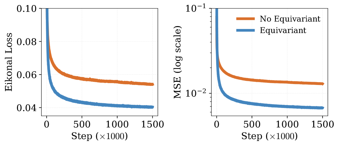
Figure 2: Comparative analysis of equivariant conditioning variables on the Style-B dataset. For non-equivariant models $\mathcal{Z}\cong\mathbb{R}^{c}$, while equivariant models use $\mathcal{Z}=SE(2)\times\mathbb{R}^{c}$.

To empirically validate the theoretical benefits of equivariance in our formulation, we conducted a controlled ablation study comparing E-NES with equivariance ($\mathcal{Z}=SE(2)\times\mathbb{R}^{c}$) against a variant without equivariance constraints ($\mathcal{Z}\cong\mathbb{R}^{c}$) on the Style-B dataset. Figure 2 illustrates consistent performance advantages with equivariance, demonstrated by lower values in both Eikonal loss and mean squared error (MSE) throughout the training process. This empirical validation substantiates our theoretical motivation for incorporating explicit equivariance constraints into the model architecture.

5.1.2 Performance Comparison

Table 1 presents a systematic comparison between E-NES and FC-DeepONet (Mei et al., 2024) across all ten OpenFWI benchmark datasets. We evaluate three configurations of E-NES: autodecoding with 100 epochs (tradeoff between computational efficiency and performance), autodecoding until convergence (optimizing for accuracy), and meta-learning (prioritizing computational efficiency).

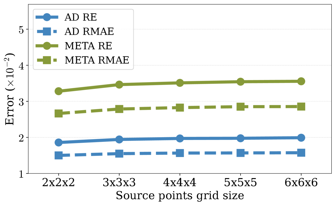
(a)

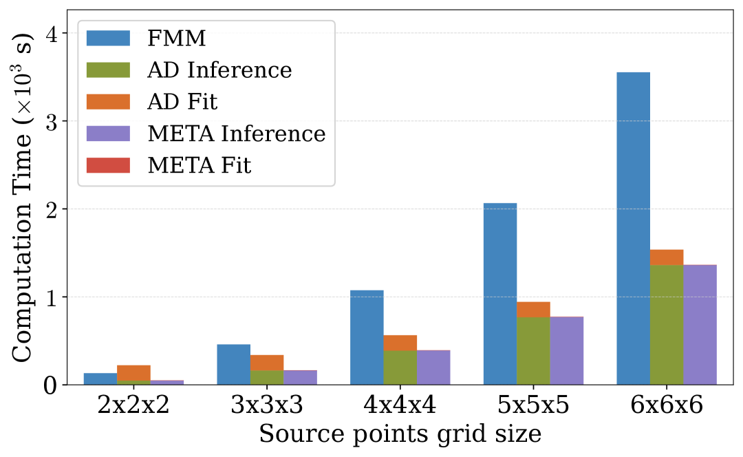
(b)

Figure 3: Scaling analysis of E-NES versus FMM on 3D OpenFWI data. (a) Both autodecoding and meta-learning maintain consistent error metrics (RE and RMAE, $\times 10^{-2}$) across increasing grid dimensions. (b) E-NES demonstrates computational advantages (seconds $\times 10^{3}$) over FMM even at minimal grid sizes, with efficiency gains amplifying as dimensions increase. Note that meta-learning fitting times (approximately 3 seconds) are barely visible in (b) due to their minimal magnitude relative to other computational times displayed.

Our results demonstrate that E-NES with full autodecoding convergence outperforms FC-DeepONet in seven out of ten datasets, with particularly substantial improvements on the more challenging variants—Style-A/B, FlatFault-B, and CurveFault-B. Even with the reduced computational budget of 100 epochs, E-NES maintains competitive performance across most datasets. The meta-learning approach, while exhibiting moderately higher error rates, delivers remarkable computational efficiency—reducing fitting time from approximately 1000 seconds to under 6 seconds per velocity field, representing a two orders of magnitude improvement.

The quantitative results are supplemented by qualitative evaluations in the Appendix (Section E.4), including visualizations of travel-time predictions and spatial error distributions across all datasets. For a more detailed analysis of the trade-off between computational efficiency and prediction accuracy, including performance with varying numbers of autodecoding epochs, we refer to the ablation studies in the Appendix (Section E.3).

5.2 Extending to 3D: Scalability Analysis

To evaluate scalability to higher dimensions, we extended the Style-B dataset into 3D by extruding the 2D velocity fields along the z-axis, allowing for controlled assessment across varying source points grid resolutions. Figure 3(a) demonstrates that both autodecoding and meta-learning approaches maintain stable error metrics as grid dimensions increase, highlighting E-NES’s effectiveness in modeling continuous fields independent of discretization resolution. Computational comparisons in Figure 3(b) reveal that E-NES maintains efficiency advantages over the Fast Marching Method (FMM) across all evaluated grid dimensions, with this advantage becoming more pronounced at larger scales.

This performance stability stems from E-NES’s continuous representation of the solution field, which adapts to the underlying physics without requiring increasingly fine discretization for differential operator approximation. The 3D experiments confirm that E-NES principles generalize effectively to higher-dimensional domains while maintaining both accuracy and computational advantages—a significant benefit for practical applications in complex settings.

6 Discussion and Future Work

In this work, we proposed a systematic approach to incorporate equivariance into neural fields and demonstrated its effectiveness through our Equivariant Neural Eikonal Solver (E-NES). Our experiments show that E-NES outperforms Neural Operator methods such as FC-DeepONet across most benchmark datasets. A key advantage of our approach is its grid-free formulation, which is particularly beneficial for gradient integration tasks and naturally extends to Riemannian manifolds. While operator-based approaches like DeepONet eliminate fitting time for conditioning variables, our meta-learning strategy achieves comparable efficiency with negligible fitting times while maintaining competitive performance. Additional comparative analyses with alternative methods are provided in the Appendix (Section E.5). For future work, we aim to extend our empirical analysis to homogeneous spaces beyond Euclidean domains, such as position-orientation spaces for modeling systems with nonholonomic constraints (particularly relevant for vehicle path planning), and hyperbolic spaces for hierarchical interpolation tasks.

Appendix A Steerability and Gradient Equivariance

Let $G$ be a Lie group acting smoothly on the Riemannian manifold $(\mathcal{M},\mathcal{G})$ by left-translations

$$L_{g}\colon\mathcal{M}\to\mathcal{M},\qquad L_{g}(p)=g\!\cdot p\,$$

and write $\mathop{}\!\mathrm{d}L_{g}(s)\colon T_{s}\mathcal{M}\to T_{gs}\mathcal{M}$ for its differential. Let $(\mathop{}\!\mathrm{d}L_{g}(s))^{*}:T_{gs}\mathcal{M}\to T_{s}\mathcal{M}$ denote the adjoint of $\mathop{}\!\mathrm{d}L_{g}(s)$ with respect to the metric $\mathcal{G}$.

Lemma A.1 (Gradient Equivariance).

Let $T_{\theta}\colon\mathcal{M}\times\mathcal{M}\times\mathscr{P}(\mathcal{Z})\to\mathbb{R}_{+}$ be a steerable conditional neural field, i.e. for all $g\in G$ and all $s,r\in\mathcal{M}$, $T_{\theta}(s,r;g\cdot z)=T_{\theta}(g^{-1}\cdot s,\,g^{-1}\cdot r;z)$. Then, for each fixed $z\in\mathcal{Z}$, fixed receiver $r\in\mathcal{M}$, and every $g\in G$,

$$\operatorname{grad}_{s}\,T_{\theta}(s,r;g\cdot z)\;=\;(\mathop{}\!\mathrm{d}L_{g^{-1}}(s))^{*}\left[\operatorname{grad}_{g^{-1}s}\,T_{\theta}(g^{-1}\cdot s,\;g^{-1}\cdot r;z)\right]\in T_{s}\mathcal{M}.$$

Proof.

By steerability, one has

$$T_{\theta}(s,r;g\cdot z)=T_{\theta}\bigl{(}L_{g^{-1}}(s),\,L_{g^{-1}}(r);z\bigr{)}.$$

Fix $r\in\mathcal{M}$ and differentiate with respect to $s$. For any $\dot{v}\in T_{s}\mathcal{M}$, the chain rule yields

$$\mathop{}\!\mathrm{d}_{s}T_{\theta}(s,r;g\cdot z)[\dot{v}]=\mathop{}\!\mathrm{d}_{g^{-1}s}T_{\theta}\bigl{(}g^{-1}\cdot s,\;g^{-1}\cdot r;z\bigr{)}\bigl{[}\mathop{}\!\mathrm{d}L_{g^{-1}}(s)[\dot{v}]\bigr{]}.$$

By the defining property of the Riemannian gradient, we have $\mathcal{G}(\operatorname{grad}f,\cdot)=\mathop{}\!\mathrm{d}f$, so that:

$$\mathcal{G}_{s}\bigl{(}\,\underbrace{\operatorname{grad}_{s}T_{\theta}(s,r;g\cdot z)}_{\in T_{s}\mathcal{M}}\,,\dot{v}\bigr{)}=\mathcal{G}_{g^{-1}s}\bigl{(}\,\underbrace{\operatorname{grad}_{g^{-1}s},T_{\theta}\bigl{(}g^{-1}\cdot s,g^{-1}\cdot r;z)}_{\in T_{g^{-1}s}\mathcal{M}}\,,\mathop{}\!\mathrm{d}L_{g^{-1}}(s)[\dot{v}]\bigr{)}.$$

This exactly characterizes the adjoint $(\mathop{}\!\mathrm{d}L_{g^{-1}}(s))^{*}$, and the result follows. ∎

Definition 4.1 (Restated).

For all $g\in G$, define the $g$-steered metric $\mathcal{G}^{g}:T\mathcal{M}\times T\mathcal{M}\to\mathbb{R}$ as:

$$\mathcal{G}^{g}_{p}\left(\dot{u},\dot{v}\right):=\mathcal{G}_{gp}\left((\mathop{}\!\mathrm{d}L_{g^{-1}}(g\cdot p))^{*}[\dot{u}],(\mathop{}\!\mathrm{d}L_{g^{-1}}(g\cdot p))^{*}[\dot{v}]\right)\quad\text{for }p\in\mathcal{M},\text{ and }\dot{u},\dot{v}\in T_{p}\mathcal{M}.$$

Proposition 4.1 (Restated).

Let $T_{\theta}:\mathcal{M}\times\mathcal{M}\times\mathscr{P}(\mathcal{Z})\to\mathbb{R}_{+}$ be a conditional neural field satisfying the steerability property (2), and let $z_{l}$ be the conditioning variable representing the solution of the eikonal equation for $v_{l}:\mathcal{M}\to\mathbb{R}_{+}^{*}$, i.e., $T_{\theta}(s,r;z_{l})\approx T_{l}(s,r)$ for $T_{l}$ satisfying Equation (1) for the velocity field $v_{l}$. Let $\mathcal{G}^{g}$ be a $g$-steered metric (Definition 4.1). Then:

1. The map $\mu:G\times(\mathcal{M}\to\mathbb{R}_{+}^{*})\to(\mathcal{M}\to\mathbb{R}_{+}^{*})$ defined by

   $$\mu(g,v_{l})(s):=\frac{1}{\bigl{\|}\operatorname{grad}_{g^{-1}s}\,T_{l}(g^{-1}\cdot s,\;g^{-1}\cdot r)\bigr{\|}_{\mathcal{G}^{g}}},$$ (6)

   where $r$ is an arbitrary point in $\mathcal{M}$, is a well-defined group action.

2. For any $g\in G$, $T_{\theta}(s,r;g\cdot z_{l})$ solves the eikonal equation with velocity field $\mu(g,v_{l})$.

Proof.

By the steerability of $T_{\theta}$, for every $g\in G$ and $s,r\in\mathcal{M}$ we have

$$T_{\theta}(s,r;g\cdot z_{l})=T_{\theta}(g^{-1}\cdot s,g^{-1}\cdot r;z_{l}).$$

Since $T_{\theta}(s,r;z_{l})\approx T_{l}(s,r)$, it follows that

$$T_{\theta}(s,r;g\cdot z_{l})\approx T_{l}(g^{-1}\cdot s,g^{-1}\cdot r).$$

Define the steered arrival time

$$T_{l}^{g}(s,r):=T_{l}(g^{-1}\cdot s,g^{-1}\cdot r).$$

We aim to show that $T_{l}^{g}$ satisfies the eikonal equation with velocity field $\mu(g,v_{l})$.

Gradient transformation.

By Lemma A.1, the gradient of $T_{l}^{g}$ is related to that of $T_{l}$ via

$$\operatorname{grad}_{s}T_{l}^{g}(s,r)=(\mathop{}\!\mathrm{d}L_{g^{-1}}(s))^{*}\left[\operatorname{grad}_{g^{-1}s}\,T_{l}(g^{-1}\cdot s,\;g^{-1}\cdot r)\right].$$

Fix $g\in G$ and write $\dot{w}=\operatorname{grad}_{g^{-1}s}T_{l}(g^{-1}\cdot s,g^{-1}\cdot r)\in T_{g^{-1}s}\mathcal{M}$. Taking the squared $\mathcal{G}$-norm we get:

$$\|\operatorname{grad}_{s}T_{l}^{g}(s,r)\|_{\mathcal{G}}^{2}=\mathcal{G}_{s}\left((\mathop{}\!\mathrm{d}L_{g^{-1}}(s))^{*}[\dot{w}],(\mathop{}\!\mathrm{d}L_{g^{-1}}(s))^{*}[\dot{w}]\right).$$

Then, for $\mathcal{G}^{g}$ defined by Definition 4.1:

$$\|\operatorname{grad}_{g^{-1}s}T_{l}(g^{-1}\cdot s,g^{-1}\cdot r)\|_{\mathcal{G}^{g}}^{2} =\mathcal{G}^{g}_{g^{-1}s}\left(\dot{w},\dot{w}\right)$$

$$=\mathcal{G}_{gg^{-1}s}\left((\mathop{}\!\mathrm{d}L_{g^{-1}}(g\cdot g^{-1}\cdot s))^{*}[\dot{w}],(\mathop{}\!\mathrm{d}L_{g^{-1}}(g\cdot g^{-1}\cdot s))^{*}[\dot{w}]\right)$$

$$=\mathcal{G}_{s}\left((\mathop{}\!\mathrm{d}L_{g^{-1}}(s))^{*}[\dot{w}],(\mathop{}\!\mathrm{d}L_{g^{-1}}(s))^{*}[\dot{w}]\right)$$

$$=\|\operatorname{grad}_{s}T_{l}^{g}(s,r)\|_{\mathcal{G}}^{2}\,.$$

By Eq. (3), we now get

$$\|\operatorname{grad}_{s}T_{l}^{g}(s,r)\|_{\mathcal{G}}=\frac{1}{\mu(g,v_{l})(s)},$$

i.e., $T_{l}^{g}$ solves the eikonal equation with velocity $\mu(g,v_{l})$.

Group action properties of $\mu$.

(1) Identity: Let $e\in G$ denote the identity. Then $e^{-1}=e$ and $\mathop{}\!\mathrm{d}L_{e}(s)=\mathrm{Id}$, hence:

$$\mathcal{G}^{e}_{s}=\mathcal{G}_{s},\qquad\mu(e,v_{l})(s)=\|\operatorname{grad}_{s}T_{l}(s,r)\|_{\mathcal{G}}^{-1}=v_{l}(s),$$

using the eikonal equation for $T_{l}$.

(2) Compatibility: For all $g,h\in G$, we show that:

$$\mu(g,\mu(h,v_{l}))=\mu(gh,v_{l}).$$

We note that left and right hand side are respectively given by

$$\mu(g,\mu(h,v_{l}))=\frac{1}{\|\operatorname{grad}_{h^{-1}g^{-1}s}T_{l}(h^{-1}g^{-1}s,h^{-1}g^{-1}r)\|_{(\mathcal{G}^{h})^{g}}}$$ (7)

and

$$\mu(gh,v_{l})=\frac{1}{\|\operatorname{grad}_{(gh)^{-1}}T_{l}((gh)^{-1}s,(gh)^{-1}r)\|_{\mathcal{G}^{gh}}}.$$ (8)

Both equations (7) and (8) are the same iff $\mathcal{G}^{gh}=(\mathcal{G}^{h})^{g}$. By Definition 4.1, it suffices to show $(\mathop{}\!\mathrm{d}L_{(gh)^{-1}})^{*}=(\mathop{}\!\mathrm{d}L_{g^{-1}})^{*}(\mathop{}\!\mathrm{d}L_{h^{-1}})^{*}$ which follows readily:

$$(\mathop{}\!\mathrm{d}L_{(gh)^{-1}})^{*}=(\mathop{}\!\mathrm{d}L_{h^{-1}}\circ\mathop{}\!\mathrm{d}L_{g^{-1}})^{*}=(\mathop{}\!\mathrm{d}L_{g^{-1}})^{*}(\mathop{}\!\mathrm{d}L_{h^{-1}})^{*}.$$

Hence, the group action $\mu$ is compatible.

∎

Corollary 4.1 (Restated).

Assume the hypotheses of Proposition 4.1, then the group action $\mu:G\times(\mathcal{M}\to\mathbb{R}_{+}^{*})\to(\mathcal{M}\to\mathbb{R}_{+}^{*})$ is given by:

1. $\mu(g,v_{l})(s)=v_{l}(g^{-1}\cdot s)$ if $G$ acts isometrically on $\mathcal{M}$.

2. $\mu(g,v_{l})(s)=\Omega(g,s)\,v_{l}(g^{-1}\cdot s)$ if $G$ acts conformally on $\mathcal{M}$ with conformal factor $\Omega(g,s)>0$, i.e., $\mathcal{G}_{gs}\left(\mathop{}\!\mathrm{d}L_{g}(s)[\dot{s}_{1}],\,\mathop{}\!\mathrm{d}L_{g}(s)[\dot{s}_{2}]\right)=\Omega(g,s)^{2}\,\mathcal{G}_{s}\left(\dot{s}_{1},\,\dot{s}_{2}\right)$, $\forall\,\dot{s}_{1},\dot{s}_{2}\in T_{s}\mathcal{M}.$

Proof.

(1) Isometric case: If $L_{g^{-1}}$ is an isometry, then $(\mathop{}\!\mathrm{d}L_{g^{-1}}(s))^{*}=(\mathop{}\!\mathrm{d}L_{g^{-1}}(s))^{-1}=\mathop{}\!\mathrm{d}L_{g}(s)$ – so that $\mathcal{G}^{p}$ is equal to the pull-back metric – and preserves inner products. Hence,

$$\bigl{\|}\dot{u}\bigr{\|}_{\mathcal{G}^{g}}=\mathcal{G}^{g}_{p}(\dot{u},\dot{u})=\mathcal{G}_{gp}(\mathop{}\!\mathrm{d}L_{g}(s)[\dot{u}],\mathop{}\!\mathrm{d}L_{g}(s)[\dot{u}])=\mathcal{G}_{p}(\dot{u},\dot{u})=\bigl{\|}\dot{u}\bigr{\|}_{\mathcal{G}}.$$

Therefore,

$$\bigl{\|}\operatorname{grad}_{s}T_{\theta}(s,r;g\cdot z_{l})\bigr{\|}_{\mathcal{G}}=\|\operatorname{grad}_{g^{-1}s}T_{\theta}(g^{-1}\cdot s,g^{-1}\cdot r;z_{l})\bigr{\|}_{\mathcal{G}^{g}}=\frac{1}{v_{l}(g^{-1}\cdot s)},$$

so $\mu(g,v_{l})(s)=v_{l}(g^{-1}\cdot s)$.

(2) Conformal case: If $L_{g}$ acts conformally with factor $\Omega(g,s)$, then for all $\dot{s}_{1},\dot{s}_{2}\in T_{s}\mathcal{M}$,

$$\mathcal{G}_{gs}\left(\mathop{}\!\mathrm{d}L_{g}(s)[\dot{s}_{1}],\,\mathop{}\!\mathrm{d}L_{g}(s)[\dot{s}_{2}]\right)=\Omega(g,s)^{2}\,\mathcal{G}_{s}\left(\dot{s}_{1},\,\dot{s}_{2}\right).$$

Hence $\mathop{}\!\mathrm{d}L_{g^{-1}}(s)$ scales lengths by $\Omega(g^{-1},s)=\Omega(g,s)^{-1}$ and its adjoint satisfies

$$(\mathop{}\!\mathrm{d}L_{g^{-1}}(s))^{*}=\Omega(g,s)^{-2}\,(\mathop{}\!\mathrm{d}L_{g^{-1}}(s))^{-1},\quad\text{because }(\mathop{}\!\mathrm{d}L_{g}(s))^{*}=\Omega(g,s)^{2}\,(\mathop{}\!\mathrm{d}L_{g}(s))^{-1}.$$

Then

$$\operatorname{grad}_{s}T_{\theta}(s,r;g\cdot z_{l})=\Omega(g,s)^{-2}\,(\mathop{}\!\mathrm{d}L_{g^{-1}}(s))^{-1}[\operatorname{grad}_{g^{-1}s}\,T_{\theta}(g^{-1}\cdot s,\;g^{-1}\cdot r;z_{l})],$$

and thus

$$\bigl{\|}\operatorname{grad}_{s}T_{\theta}(s,r;g\cdot z_{l})\bigr{\|}_{\mathcal{G}}=\frac{1}{\Omega(g,s)\,v_{l}(g^{-1}\cdot s)}.$$

Therefore $\mu(g,v_{l})(s)=\Omega(g,s)\,v_{l}(g^{-1}\cdot s)$. ∎

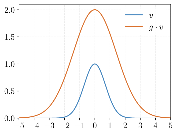
Figure 4: Example of conformal group action on $v(s)=e^{-s^{2}}$.

As an example of an isometric action, consider 2D rotations with $G=SO(2)$ acting on $\mathcal{M}=\mathbb{R}^{2}$. In Figure 1, given a velocity field $v(s)$ and its corresponding conditioning variable $z$, the transformed variable $R_{\pi/6}\cdot z$ encodes the velocity field $v(R_{5\pi/6}s)$. Similarly, as an example of a conformal action, consider the positive scaling group $G=\mathbb{R}^{*}_{+}$ acting on $\mathcal{M}=\mathbb{R}$. In the graph shown in Figure 4, given a velocity field $v(s)$ encoded by $z$, the scaled conditioning variable $2\cdot z$ encodes the velocity field $2\,v(s/2)$.

Remark A.1 (Implementation in Euclidean Coordinates).

In local coordinates, the metric tensor $\mathcal{G}_{p}$ at any point $p\in\mathcal{M}$ is represented by a symmetric positive-definite matrix, which induces an inner product on the tangent space $T_{p}\mathcal{M}$. Specifically, for any tangent vectors $\dot{p}_{1},\dot{p}_{2}\in T_{p}\mathcal{M}$, the inner product is given by $\mathcal{G}_{p}(\dot{p}_{1},\dot{p}_{2})=\langle\dot{p}_{1},\dot{p}_{2}\rangle_{\mathcal{G}}=\dot{p}_{1}^{\top}\mathcal{G}_{p}\dot{p}_{2}$, and the corresponding norm is defined as $\left\lVert\dot{p}_{1}\right\rVert_{\mathcal{G}}=\sqrt{\langle\dot{p}_{1},\dot{p}_{1}\rangle_{\mathcal{G}}}$.

Moreover, in local coordinates, the Riemannian gradient is related to that of the Euclidean gradient $\nabla f$ via the inverse metric tensor: $\operatorname{grad}f(p)=\mathcal{G}_{p}^{-1}\nabla f(p)$ (Absil et al., 2008). If $\mathcal{M}$ is embedded in a Euclidean space, then the norm of the Riemannian gradient can be computed as $\left\lVert\operatorname{grad}f\right\rVert_{\mathcal{G}}=\left\lVert\nabla f\right\rVert_{\mathcal{G}^{-1}}$, and the adjoint can be computed as $(\mathop{}\!\mathrm{d}L_{g^{-1}}(s))^{*}=\mathcal{G}_{s}^{-1}(\mathop{}\!\mathrm{d}L_{g^{-1}}(s))^{T}\mathcal{G}_{g^{-1}s}$.

Therefore, the group action $\mu:G\times(\mathcal{M}\to\mathbb{R}_{+}^{*})\to(\mathcal{M}\to\mathbb{R}_{+}^{*})$ in local coordinates is given by:

$$\mu(g,v_{l})(s)=\bigl{\|}\nabla_{g^{-1}s}T_{l}\bigl{(}g^{-1}\cdot s,g^{-1}\cdot r\bigr{)}\bigr{\|}_{\widetilde{\mathcal{G}}^{g}}^{-1},$$

where $r$ is an arbitrary point in $\mathcal{M}$, and $\widetilde{\mathcal{G}}^{g}:T_{p}\mathcal{M}\times T_{p}\mathcal{M}\to\mathbb{R}$ is the local coordinated expression of the $g$-steered metric given by

$$\widetilde{\mathcal{G}}^{g}_{p}:=\mathop{}\!\mathrm{d}L_{g^{-1}}(g\cdot p)\mathcal{G}_{gp}^{-1}(\mathop{}\!\mathrm{d}L_{g^{-1}}(g\cdot p))^{T}\quad\text{for any }p\in\mathcal{M}.$$

Remark A.2 (Relation to pull-back metric).

If $\mathcal{G}$ is isometric or conformal, then the $g$-steered metric is the pull-back metric $\mathcal{G}^{g}=(L_{g})^{*}\mathcal{G}$ and one directly has

$$\mathcal{G}^{g_{1}g_{2}}=(\mathcal{G}^{g_{2}})^{g_{1}}\Rightarrow\mu(g_{1}g_{2},v_{l})=\mu(g_{1},\mu(g_{2},v_{1})).$$

Appendix B Computing Invariants via Moving Frame

B.1 Preliminaries

In this section, we present the essential mathematical foundations of the Moving Frame method, following Olver (2001); Sangalli et al. (2023). For a comprehensive treatment, we refer readers to Olver (2011, 1995).

Let $\mathcal{M}$ be an $m$-dimensional smooth manifold and $G$ be an $r$-dimensional Lie group acting on $\mathcal{M}$. A (right) moving frame is a smooth equivariant map $\rho:\mathcal{M}\to G$ satisfying $\rho(g\cdot p)=\rho(p)\cdot g^{-1}$ for all $g\in G$ and $p\in\mathcal{M}$. Every moving frame $\rho$ induces a canonicalization function $k:\mathcal{M}\to\mathcal{M}$ defined by

$$k(p)=\rho(p)\cdot p,$$

which is $G$-invariant:

$$\forall p\in\mathcal{M},\;g\in G,\quad k(g\cdot p)=\rho(g\cdot p)\cdot g\cdot p=\rho(p)\cdot p=k(p).$$

The existence of moving frames is characterized by the following fundamental result:

Theorem B.1 (Existence of moving frame; see Olver (2001)).

A moving frame exists in a neighborhood of a point $p\in\mathcal{M}$ if and only if $G$ acts freely and regularly near $p$.

Moving frames can be constructed via cross-sections to group orbits. A cross-section to the group orbits is a submanifold $K\subseteq\mathcal{M}$ of complementary dimension to the group (i.e., $\dim K=m-r$) that intersects each orbit transversally at exactly one point.

Theorem B.2 (Moving frame from cross-section; see Olver (2001)).

If $G$ acts freely and regularly on $\mathcal{M}$, then given a cross-section $K$ to the group orbits, for each $p\in\mathcal{M}$ there exists a unique element $g_{p}\in G$ such that $g_{p}\cdot p\in K$. The function $\rho:\mathcal{M}\to G$ mapping $p$ to $g_{p}$ is a moving frame.

While any regular Lie group action admits multiple local cross-sections, coordinate cross-sections (obtained by fixing $r$ of the coordinates) are particularly useful for determining fundamental invariants of $\mathcal{M}$ with regards to $G$.

Theorem B.3 (Fundamental invariants via coordinate cross-sections; see Olver (2001)).

Given a free, regular Lie group action and a coordinate cross-section $K$, let $\rho$ be the associated moving frame. Then the non-constant coordinates of the canonicalization function image

$$k(p)=\rho(p)\cdot p\in K$$

form a complete system of functionally independent invariants.

Moreover, this theorem aligns with the classical result on the structure and separation properties of invariants:

Theorem B.4 (Existence of Fundamental Invariants; see (Olver, 1995)).

Let $G$ be a Lie group acting freely and regularly on an $m$-dimensional manifold $\mathcal{M}$ with orbits of dimension $s$. Then, for each point $p\in\mathcal{M}$, there exist $m-s$ functionally independent invariants $I_{1},\ldots,I_{m-s}$ defined on a neighborhood $U$ of $p$ such that any other invariant $I$ on $U$ can be expressed as $I=H(I_{1},\ldots,I_{m-s})$ for some function $H$. Moreover, these invariants separate orbits: two points $y,z\in U$ lie in the same orbit if and only if $I_{\upsilon}(y)=I_{\upsilon}(z)$ for all $\upsilon=1,\ldots,m-s$.

These foundational results—existence, construction via cross-sections, and the properties of invariants—underlie all moving-frame computations and guarantee that one obtains a complete, orbit-separating set of invariants.

B.2 Canonicalization via latent-pose extension

Theorem 4.1 (Restated).

Let $G$ be a Lie group acting smoothly (but not necessarily freely) on each Riemannian manifold $\mathcal{M}_{i}$ via $\delta_{i}:G\times\mathcal{M}_{i}\to\mathcal{M}_{i}$, for $i=1,\dots,m$, and hence diagonally on

$$\Pi=\mathcal{M}_{1}\times\cdots\times\mathcal{M}_{m},\quad\delta\bigl{(}g,(p_{1},\dots,p_{m})\bigr{)}=\bigl{(}\delta_{1}(g,p_{1}),\dots,\delta_{m}(g,p_{m})\bigr{)}.$$

On the augmented space $\macc@depth\char 1\relax\frozen@everymath{\macc@group}\macc@set@skewchar\macc@nested@a 111{\Pi}=\Pi\times G$, define $\macc@depth\char 1\relax\frozen@everymath{\macc@group}\macc@set@skewchar\macc@nested@a 111{\delta}\bigl{(}h,(p_{1},\dots,p_{m},g)\bigr{)}=\bigl{(}\delta(h,(p_{1},\dots,p_{m})),\;h\,g\bigr{)}.$ Then:

1. $\macc@depth\char 1\relax\frozen@everymath{\macc@group}\macc@set@skewchar\macc@nested@a 111{\delta}$ is free.

2. A moving frame is given by $\rho:\macc@depth\char 1\relax\frozen@everymath{\macc@group}\macc@set@skewchar\macc@nested@a 111{\Pi}\to G$, such that $\rho(p_{1},\dots,p_{m},g)=g^{-1}$.

3. The set $\left\{\delta_{i}(g^{-1},p_{i})\right\}_{i=1}^{m}$ forms a complete collection of functionally independent invariants of the action $\macc@depth\char 1\relax\frozen@everymath{\macc@group}\macc@set@skewchar\macc@nested@a 111{\mu}$.

Proof.

(1) Freeness: Fix $(p_{1},\dots,p_{m},g)\in\macc@depth\char 1\relax\frozen@everymath{\macc@group}\macc@set@skewchar\macc@nested@a 111{\Pi}$. Its isotropy subgroup is

$$G_{(p_{1},\dots,p_{m},g)}=\bigl{\{}\,h\in G:\;\delta(h,(p_{1},\dots,p_{m}))=(p_{1},\dots,p_{m}),\;h\,g=g\bigr{\}}.$$

Hence

$$G_{(p_{1},\dots,p_{m},g)}=G_{p_{1}}\cap\cdots\cap G_{p_{m}}\cap G_{g}.$$

where $G_{p_{i}}$ denotes the isotropy subgroup of $p_{i}$ under $\delta_{i}$, and $G_{g}$ is the isotropy subgroup of $g\in G$ under left multiplication. Since $hg=g$ implies $h=e$ in a group, we have $G_{g}=\{e\}$. Thus, the intersection is trivial, and $\macc@depth\char 1\relax\frozen@everymath{\macc@group}\macc@set@skewchar\macc@nested@a 111{\mu}$ defines a free action.

(2) Moving frame existence: Because $\macc@depth\char 1\relax\frozen@everymath{\macc@group}\macc@set@skewchar\macc@nested@a 111{\delta}$ is free and regular, Theorem B.1 guarantees a unique smooth equivariant map

$$\rho:\macc@depth\char 1\relax\frozen@everymath{\macc@group}\macc@set@skewchar\macc@nested@a 111{\Pi}\to G$$

associated to the cross-section $K=\{(p_{1},\ldots,p_{m},g)\in\macc@depth\char 1\relax\frozen@everymath{\macc@group}\macc@set@skewchar\macc@nested@a 111{\Pi}:g=e\}$. A direct check shows

$$\rho(p_{1},\dots,p_{m},g)=g^{-1},$$

and one verifies equivariance

$$\rho\bigl{(}\macc@depth\char 1\relax\frozen@everymath{\macc@group}\macc@set@skewchar\macc@nested@a 111{\delta}(h,(p_{1},\dots,p_{m},g))\bigr{)}=(h\,g)^{-1}=g^{-1}h^{-1}=\rho(p_{1},\dots,p_{m},g)\,h^{-1}.$$

(3) Functional independence and completeness: The canonicalization map $k(p_{1},\dots,p_{m},g)=\macc@depth\char 1\relax\frozen@everymath{\macc@group}\macc@set@skewchar\macc@nested@a 111{\delta}(\rho(p_{1},\dots,p_{m},g),(p_{1},\dots,p_{m},g))\in K$ gives

$$k(p_{1},\dots,p_{m},g) =\macc@depth\char 1\relax\frozen@everymath{\macc@group}\macc@set@skewchar\macc@nested@a 111{\delta}(g^{-1},(p_{1},\dots,p_{m},g))$$

$$=\bigl{(}\delta_{1}(g^{-1},p_{1}),\dots,\delta_{m}(g^{-1},p_{m}),\,e\bigr{)}.$$

By Theorem B.3, the nonconstant coordinates $\delta_{i}(g^{-1},p_{i})$ are functionally independent and generate all invariants of $\macc@depth\char 1\relax\frozen@everymath{\macc@group}\macc@set@skewchar\macc@nested@a 111{\delta}$. ∎

Appendix C Training and Inference Details

C.1 Training

Autodecoding.

In autodecoding, we jointly optimize both the network parameters $\theta$ and the latent conditioning variables ${z_{i}}$ across the dataset. As detailed in Algorithm 1, this approach yields a tighter fit to the eikonal equation, at the expense of longer training times. Empirically, we observe that convergence on the validation set requires between 250 and 500 fitting epochs.

Algorithm 1 Autodecoding Training

1:Velocity fields $\mathcal{V}=\{v_{l}\}_{l=1}^{K}$, epochs $num\_epochs$, batch size $B$, pairs per field $N_{sr}$, learning rate $\eta$

2:Randomly initialize shared base network $T_{\theta}$

3:Initialize latents $z_{l}\leftarrow\{(g_{i},\mathbf{c}_{i})\}_{i=1}^{N}$ for all velocity fields

4:for $epochs=1$ to $num\_epochs$ do

5:  while dataloader not empty do

6:   Sample batch $\mathcal{B}=\{(s_{i,j},r_{i,j},v_{i}(s_{i,j}),v_{i}(r_{i,j}))\}_{i=1,j=1}^{B,N_{sr}}$

7:   Compute loss $L(\theta,\{z_{i}\}_{i=1}^{B},\mathcal{B})$ (see Equation 5)

8:   Update $\theta\leftarrow\theta-\eta\,\nabla_{\theta}L$

9:   Update each $z_{i}\leftarrow z_{i}-\eta\,\nabla_{z_{i}}L$

10:  end while

11:end for

12:Trained $\theta$ and latents $\{z_{l}\}_{l=1}^{K}$

Meta-learning.

Our meta-learning framework separates training into two loops: an inner loop for optimizing latents and an outer loop for updating network parameters. Algorithm 2 summarizes this bi-level optimization procedure.

Algorithm 2 Meta-learning Training

1:Velocity fields $\mathcal{V}=\{v_{l}\}_{l=1}^{K}$, outer epochs $num\_epochs$, inner steps $S$, batch size $B$, pairs per field $N_{sr}$, learning rates $\eta_{\theta},\eta_{\text{SGD}}$

2:Initialize shared base network $T_{\theta}$ (optionally pretrained), and learnable learning rate $\eta_{z}$.

3:for $epochs=1$ to $num\_epochs$ do

4:  while dataloader not empty do

5:   Sample batch of velocity fields $\{v_{i}\}_{i=1}^{B}\subseteq\mathcal{V}$

6:   Initialize latents ${z_{i}^{(0)}}$ for each $v_{i}$

7:   for $t=1$ to $S$ do $\triangleright$ Inner loop: Update latents

8:     Sample $N_{sr}$ source–receiver pairs $\{(s_{i,j}^{(t-1)},r_{i,j}^{(t-1)})\}_{j=1}^{N_{sr}}\subset\mathcal{M}^{2}$, for each $v_{i}$

9:     Construct batch $\mathcal{B}^{(t-1)}=\{(s_{i,j}^{(t-1)},r_{i,j}^{(t-1)},v_{i}(s_{i,j}^{(t-1)}),v_{i}(r_{i,j}^{(t-1)}))\}_{i=1,j=1}^{B,N_{sr}}$

10:     Compute $\widetilde{L}(\theta,\{z_{i}^{(t-1)}\}_{i=1}^{B},\mathcal{B}^{(t-1)})$

11:     Update each $z_{i}^{(t)}\leftarrow z_{i}^{(t-1)}-\eta_{z}\,\nabla_{z_{i}}\widetilde{L}$

12:   end for

13:   Sample $N_{sr}$ source–receiver pairs $\{(s_{i,j}^{(S)},r_{i,j}^{(S)})\}_{j=1}^{N_{sr}}\subset\mathcal{M}^{2}$, for each $v_{i}$

14:   Construct batch $\mathcal{B}^{(S)}=\{(s_{i,j}^{(S)},r_{i,j}^{(S)},v_{i}(s_{i,j}^{(S)}),v_{i}(r_{i,j}^{(S)}))\}_{i=1,j=1}^{B,N_{sr}}$

15:   Compute $\widetilde{L}_{meta}(\theta)=\widetilde{L}(\theta,\{z_{i}^{(S)}\}_{i=1}^{B},\mathcal{B}^{(S)})$

16:   Update $\theta\leftarrow\theta-\eta_{\theta},\nabla_{\theta}\widetilde{L}_{meta}$

17:   Update $\eta_{z}\leftarrow\eta_{z}-\eta_{\text{SGD}}\,\nabla_{\eta_{z}}\widetilde{L}_{meta}$

18:  end while

19:end for

20:Trained $\theta$

By leveraging meta-learning, we achieve significantly faster fitting and impose additional structure on the latent space (Knigge et al., 2024). However, as noted by Dupont et al. (2022), the small number of inner-loop updates typically used on meta-learning can restrict expressivity. To mitigate this, we initialize the network with weights pretrained via autodecoding, which accelerates convergence and often leads to better local minima (see Section E.1).

In our implementation, we utilize an alternative loss function $\widetilde{L}$ in place of the original loss defined in Equation 5. Specifically, $\widetilde{L}$ employs the log-hyperbolic cosine loss $\log(\cosh(x))$ (Jeendgar et al., 2022), as a differentiable substitute for the absolute value term in Equation 5. This substitution is critical for effective meta-learning, as the log-cosh function provides a smooth approximation to the absolute value while maintaining convexity and ensuring well-behaved gradients throughout its domain. The differentiability properties of this function enable us to obtain high-quality higher-order derivatives, which are essential for the backpropagation process through all inner optimization steps, as outlined in lines 15 and 16 of Algorithm 2.

C.2 Inference

Solving for new velocity fields.

Given a new set of velocity fields, we will obtain their corresponding latent representation as follows:

• Autodecoding: we perform Algorithm 1 using the frozen weights $\theta^{*}$, i.e., we do not perform steps 1 and 7.

• Meta-learning: we perform the inner loop of the Algorithm 2 using frozen weights $\theta^{*}$, i.e., we do steps 5 to 11.

Execution of bidirectional backward integration.

As stated in Section 4, given the solution of the eikonal equation, you can obtain the shortest path between two points under the given velocity via backward integration. Indeed, we perform SGD over the normalized gradients $\|\operatorname{grad}_{s}T(s,r)\|_{\mathcal{G}}\,\operatorname{grad}_{s}T(s,r)$ (Bekkers et al., 2015). Furthermore, as shown in Ni and Qureshi (2023), our model’s symmetry behavior allows us to perform gradient steps bidirectionally from source to receiver and from receiver to source. Hence, we compute the final path solution bidirectionally using iterative Riemannian Gradient Descent (Absil et al., 2008) by updating the source and receiver points as follows, where $\alpha\in\mathbb{R}$ is a step size hyperparameter.

$$\begin{cases}s^{(t)}\leftarrow R_{s^{(t-1)}}\left(-\alpha\,\|\operatorname{grad}_{s}T_{\theta^{*}}(s^{(t-1)},r^{(t-1)};z_{l})\|_{\mathcal{G}}\,\operatorname{grad}_{s}T_{\theta^{*}}(s^{(t-1)},r^{(t-1)};z_{l})\right),\\ r^{(t)}\leftarrow R_{r^{(t-1)}}\left(-\alpha\,\|\operatorname{grad}_{r}T_{\theta^{*}}(s^{(t-1)},r^{(t-1)};z_{l})\|_{\mathcal{G}}\,\operatorname{grad}_{r}T_{\theta^{*}}(s^{(t-1)},r^{(t-1)};z_{l})\right),\end{cases}$$ (9)

where $R_{p}:T_{p}\mathcal{M}\to\mathcal{M}$ is a retraction at $p\in\mathcal{M}$. The retraction mapping will provide a notion of moving in the direction of a tangent vector, while staying on the manifold:

Definition C.1 (Retraction; see Absil et al. (2008)).

A retraction on a manifold $\mathcal{M}$ is a smooth mapping $R$ from the tangent bundle $T\mathcal{M}$ onto $\mathcal{M}$ with the following properties. Let $R_{p}$ denote the restriction of $R$ to $T_{p}\mathcal{M}$.

• $R_{p}(\dot{0}_{p})=p$, where $\dot{0}_{p}$ denotes the zero element of $T_{p}\mathcal{M}$.

• With the canonical identification $T_{\dot{0}_{p}}T_{p}\mathcal{M}\simeq T_{p}\mathcal{M}$, $R_{p}$ satisfies

  $$\mathop{}\!\mathrm{d}R_{p}(\dot{0}_{p})=\mathrm{id}_{T_{p}\mathcal{M}},$$

  where $\mathrm{id}_{T_{p}\mathcal{M}}$ denotes the identity mapping on $T_{p}\mathcal{M}$.

Appendix D Experimental Details

This section presents the comprehensive training and validation hyperparameters employed in the experiments described in Section 5. All experiments were conducted using a single NVIDIA H100 GPU.

D.1 2D OpenFWI Experiments

Model Architecture.

Our invariant cross-attention implementation utilizes a hidden dimension of 128 with 3 attention heads. The conditioning variables are defined as $z\in\mathcal{P}(\mathcal{Z})$ with cardinality $|z|=9$, where $\mathcal{Z}=SE(2)\times\mathbb{R}^{32}$ for each velocity field. We initialize the pose component of the latents—derived from $SE(2)=\mathbb{R}^{2}\times S^{1}$—at equidistant positions in $\mathbb{R}^{2}$, with orientations randomly sampled from a uniform distribution over $[-\pi,\pi)$. The context component of the latents is initialized as constant unit vectors.

For embedding the invariants, we employ RFF-Net, a variant of Random Fourier Features with trainable frequency parameters. This approach enhances training robustness with respect to hyperparameter selection. Following the methodology of Wessels et al. (2024), we implement two distinct RFF embeddings: one for the value function and another for the query function of the cross-attention mechanism. The frequency parameters are initialized to 0.05 for the query function and 0.2 for the value function.

Dataset Configuration.

For each OpenFWI dataset, we sample 600 velocity fields for training and 100 for validation. We further divide the training set into 500 fields for training and 100 fields for validation. For each velocity field, we uniformly sample 20,480 coordinates, producing 10,240 pairs per velocity field. Each batch comprises two velocity fields with 5,120 source-receiver pairs per field.

Training Protocol.

The autodecoding phase consists of 3,000 epochs, while the meta-learning phase comprises 500 epochs. To mitigate overfitting, we report results based on the model that performs optimally on the validation set. Under this criterion, the effective training duration for autodecoding averages approximately 920 epochs (3.6 hours per dataset), while meta-learning averages 440 epochs (17.8 hours per dataset).

SE(2) Optimization with Pseudo-Exponential Map.

For optimizing parameters in $SE(2)=\mathbb{R}^{2}\times S^{1}$, we employ a standard simplification of Riemannian optimization for affine groups, known as parameterization via the “pseudo-exponential map.” This approach substitutes the exponential map of $SE(n)=\mathbb{R}^{n}\rtimes SO(n)$ with the exponential map of $\mathbb{R}^{n}\times SO(n)$ (Solà et al., 2021; Claraco, 2022). This technique is applied in both autodecoding and meta-learning phases, though with different optimizers as detailed below.

Autodecoding Optimization Strategy.

For autodecoding, we optimize all parameters using the Adam optimizer with different learning rates for each component. The model parameters are trained with a learning rate of $10^{-4}$. For the latent variables, context vectors use a learning rate of $10^{-2}$, while pose components in $SE(2)$ are optimized with a learning rate of $10^{-3}$. Both latent variable components (context and pose) are optimized using Adam.

Meta-learning Configuration.

For meta-learning, we jointly optimize the model parameters $\theta$ and inner loop learning rates $\eta_{z}$ using Adam with a cosine scheduler. This scheduler implements a single cycle with an initial learning rate of $10^{-4}$ and a minimum learning rate of $10^{-6}$. For the SGD inner loop optimization, we initialize the learning rates at 30 for context vectors and 2 for pose components, executing 5 optimization steps in the inner loop.

D.2 3D OpenFWI Experiments

Model Architecture.

For the 3D experiments, we adapt the architecture described in the 2D case with several key modifications. Most notably, we reduce the cross-attention mechanism to a single head rather than the three employed in the 2D experiments. Additionally, we utilize a set of eight elements in $\mathcal{Z}=SE(3)\times\mathbb{R}^{32}$ as conditioning variables instead of the nine used in the 2D case.

Pose Representation.

While we maintain the same general approach for pose optimization as in the 2D experiments, the 3D case requires parameterization of $SE(3)$ rather than $SE(2)$. We employ the pseudo-exponential map as described previously, but with an important distinction in the rotation component. Specifically, we parameterize the $SO(3)$ component using Euler angles.

Training and Optimization.

All other aspects of the training procedure—including dataset configuration, optimization strategies, learning rates, and epoch counts—remain consistent with those detailed in the 2D experiments. We maintain the same distinction between optimization approaches in autodecoding (Adam for all parameters) and meta-learning (Adam for model parameters in the outer loop, SGD for latent variables in the inner loop). This consistency allows for direct comparison between 2D and 3D experimental results while accounting for the specific requirements of 3D modeling.

Appendix E Additional results

E.1 Impact of Autodecoding Pretraining on Meta-Learning Performance

This section examines the effectiveness of initializing meta-learning with parameters derived from standard autodecoding pretraining. We present a comparative analysis using the Style-A and CurveVel-A 2D OpenFWI datasets, evaluating performance through both eikonal loss and mean squared error (MSE) metrics throughout the training process.

Figure 5 illustrates the training dynamics across both initialization strategies. Our results demonstrate that utilizing pretrained model parameters from the autodecoding phase substantially enhances convergence characteristics in two critical dimensions. First, pretrained initialization enables significantly faster convergence, reducing the number of required epochs to reach performance plateaus. Second, and more importantly, this approach allows the optimization process to achieve superior local minima compared to random initialization.

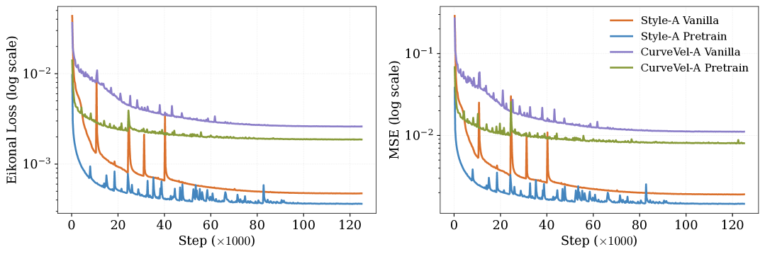
Figure 5: Comparative analysis of meta-learning convergence with pretrained versus random initialization on Style-A and CurveVel-A OpenFWI datasets.

These findings highlight a fundamental efficiency in our methodology: by leveraging pretrained autodecoding parameters, the meta-learning phase is effectively transformed from learning from scratch to a targeted adaptation task. Specifically, the pretrained model has already established a robust conditional neural field representation of the underlying physics. The subsequent meta-learning process then primarily needs to adapt this existing representation to interpret conditioning variables obtained through just 5 steps of SGD, rather than those refined over 500 epochs of autodecoding. This represents a significant computational advantage, as the meta-learning algorithm can focus exclusively on learning the mapping between rapidly-obtained SGD variables and the already-established neural field, rather than simultaneously learning both the field representation and the optimal conditioning.

E.2 Comprehensive Grid Evaluation of OpenFWI Performance

In Section 5, we evaluated E-NES performance on the OpenFWI benchmark following the methodology established by Mei et al. (2024), which utilizes four equidistant source points at the top of the velocity fields and measures predicted travel times from these sources to all 70×70 receiver coordinates. This approach allows direct comparison with both the Fast Marching Method (FMM) and the FC-DeepOnet model (Mei et al., 2024).

To validate the robustness and generalizability of our approach, we conducted additional experiments using a substantially denser sampling protocol—specifically, a uniform 14×14 source point grid similar to that employed by Grubas et al. (2023). As demonstrated in Table 2, E-NES maintains performance metrics comparable to those presented in Table 1, despite the significant increase in source points and resulting source-receiver pairs.

Table 2: Performance on OpenFWI datasets on a $14\times 14$ grid of source points.

	Autodecoding (100 epochs)			Autodecoding (convergence)			Meta-learning
Dataset	RE ($\downarrow$)	RMAE ($\downarrow$)	Fitting (s)	RE ($\downarrow$)	RMAE ($\downarrow$)	Fitting (s)	RE ($\downarrow$)	RMAE ($\downarrow$)	Fitting (s)
FlatVel-A	0.01023	0.00827	223.31	0.00624	0.00509	1010.90	0.01304	0.01003	5.92
CurveVel-A	0.01438	0.01139	222.72	0.01069	0.00841	1009.67	0.02460	0.01878	5.91
FlatFault-A	0.01050	0.00751	222.61	0.00744	0.00510	1014.45	0.01749	0.01255	5.92
CurveFault-A	0.01380	0.00976	222.89	0.01088	0.00745	1007.97	0.02471	0.01807	5.92
Style-A	0.00962	0.00785	222.00	0.00795	0.00646	783.13	0.01326	0.01036	5.92
FlatVel-B	0.01988	0.01586	222.74	0.01178	0.00906	786.48	0.03077	0.02474	5.91
CurveVel-B	0.04291	0.03349	222.97	0.03297	0.02528	1010.70	0.04977	0.03930	5.90
FlatFault-B	0.01889	0.01413	222.70	0.01557	0.01147	898.28	0.02998	0.02214	5.93
CurveFault-B	0.02244	0.01728	222.89	0.01991	0.01537	561.22	0.03824	0.02945	5.89
Style-B	0.01061	0.00860	221.90	0.00984	0.00798	1120.09	0.01566	0.01227	5.90

This consistency across sampling densities provides strong evidence that E-NES effectively captures the underlying travel-time function for arbitrary point pairs throughout the domain. We attribute this capability to two key architectural decisions in our approach. First, the grid-free architecture allows the model to operate on continuous spatial coordinates rather than discretized grid positions. Second, our training methodology leverages physics-informed neural network (PINN) principles rather than relying on numerical solver supervision as implemented in Mei et al. (2024). This physics-based learning approach enables E-NES to internalize the governing eikonal equation, resulting in a more generalizable representation of travel-time fields that remains accurate across varying evaluation protocols.

E.3 Ablation Study: Impact of Autodecoding Fitting Epochs

This section presents a systematic analysis of how the number of autodecoding fitting epochs affects model performance and computational efficiency. We evaluate the E-NES model on the 2D-OpenFWI datasets across both grid configurations described in Section E.2, measuring performance in terms of Relative Error while tracking computational costs. Additionally, we provide a comparative analysis between the standard autodecoding approach and our meta-learning methodology.

Figures 6 and 7 illustrate the relationship between fitting time, number of epochs, and model performance across all datasets. Our analysis reveals that most datasets reach optimal solution convergence at approximately 400 autodecoding fitting epochs. Performance improvements beyond this threshold exhibit diminishing returns relative to the additional computational investment required. Notably, approximately 100 autodecoding epochs represents an effective compromise between computational efficiency and performance quality.

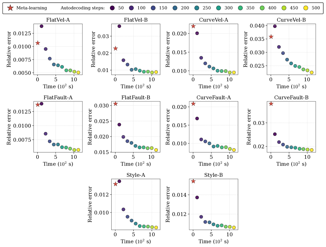
Figure 6: Comparative analysis of Relative Error versus computational time for the 4-source configuration across all datasets. Circular markers represent autodecoding performance at varying epoch counts (color-coded from 50 to 500 epochs), while the star marker indicates meta-learning performance.

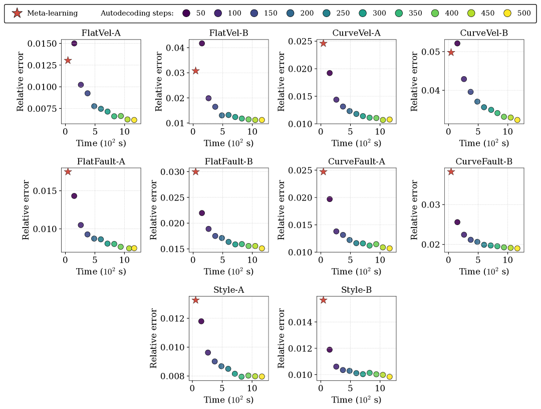
Figure 7: Comparative analysis of Relative Error versus computational time for the dense 14×14 source grid configuration. Circular markers represent autodecoding performance at varying epoch counts (color-coded from 50 to 500 epochs), while the star marker indicates meta-learning performance.

The meta-learning approach demonstrates remarkable efficiency advantages. With negligible fitting times compared to standard autodecoding, meta-learning achieves performance levels comparable to 50-100 epochs of autodecoding for the FlatVel-A/B and CurveVel-A/B datasets. This represents a substantial reduction in computational requirements while maintaining acceptable performance characteristics.

These findings suggest that practitioners can optimize computational resource allocation by selecting the appropriate training approach based on their specific performance requirements and computational constraints. For applications where rapid deployment is critical, meta-learning offers significant advantages, while applications demanding maximum accuracy may benefit from extended autodecoding training, with the optimal epoch count determined by performance saturation points identified in our analysis.

E.4 Qualitative Analysis of Travel-Time Predictions

This section provides a visual assessment of the E-NES model’s performance as quantitatively reported in Table 1. For each dataset in the 2D-OpenFWI benchmark, we present a representative velocity field alongside the corresponding ground-truth and predicted travel-time surfaces. Additionally, we visualize the spatial distribution of relative error to facilitate the identification of regions where prediction accuracy varies.

Figures 8 and 9 demonstrate the E-NES model’s capacity to accurately reconstruct travel-time functions across diverse geological scenarios. Particularly noteworthy is the model’s performance on the challenging CurveFault-A/B and Style-A/B datasets, where the travel-time functions exhibit complex wavefront behaviors including caustic singularities—regions. At these caustics, seismic-ray trajectories intersect each other, forming singularity zones where gradients are discontinuous.

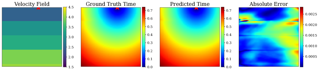
(a) Results for FlatVel-A

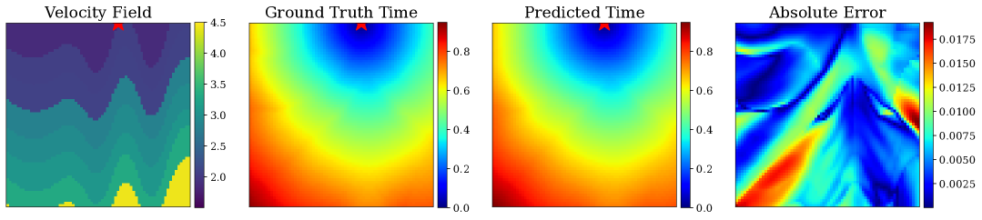
(b) Results for CurveVel-A

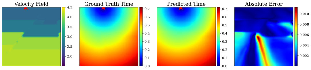
(c) Results for FlatFault-A

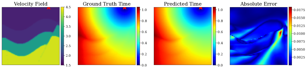
(d) Results for CurveFault-A

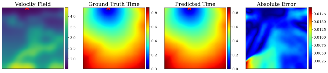
(e) Results for Style-A

Figure 8: Comparative visualization of E-NES predicted travel-times against reference solutions for OpenFWI type B datasets. Each panel displays the velocity field (left), ground-truth travel-time surface (center-left), E-NES predicted travel-time surface (center-right), and relative error distribution (right). The red star denotes the source point location from which wavefronts propagate.

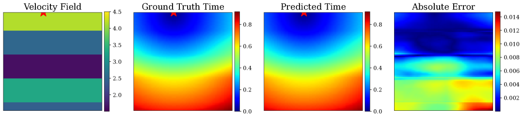
(a) Results for FlatVel-B

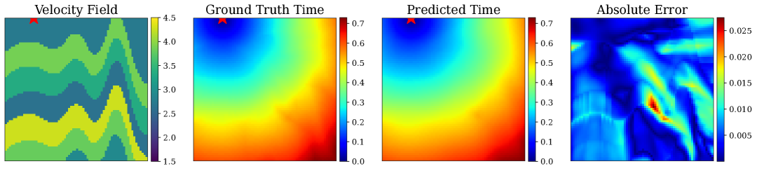
(b) Results for CurveVel-B

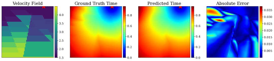
(c) Results for FlatFault-B

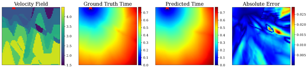
(d) Results for CurveFault-B

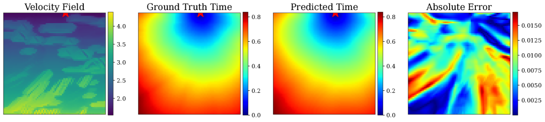
(e) Results for Style-B

Figure 9: Comparative visualization of E-NES predicted travel-times against reference solutions for OpenFWI type A datasets. Each panel displays the velocity field (left), ground-truth travel-time surface (center-left), E-NES predicted travel-time surface (center-right), and relative error distribution (right). The red star denotes the source point location from which the wavefronts propagate.

E.5 Extended Discussion

In this section, we expand our analysis to consider the relative merits of conditional versus unconditional neural field approaches for solving the eikonal equation. We intentionally excluded comparisons against unconditional neural field-based eikonal equation solvers from our main experimental results, as these comparisons require additional context to interpret appropriately.

Unconditional neural fields typically outperform conditional neural fields in both solution accuracy and inference speed for individual problem instances. This performance gap stems from the fundamental nature of the task: training an unconditional neural field essentially constitutes an overfitting problem, where even a modest MLP architecture can achieve high accuracy on a single velocity field. In contrast, conditional neural fields must generalize across multiple instances, effectively learning a mapping from conditioning variables to solution fields rather than memorizing a single solution.

However, this performance advantage diminishes significantly when considering parameter scalability across multiple velocity fields. The unconditional approach (e.g., a standard Neural Eikonal Solver) requires approximately 17,558 parameters per velocity field (Grubas et al., 2023), as it necessitates training an entirely new network for each travel-time solution. In contrast, our E-NES approach maintains a fixed baseline of 64,895 parameters for the core network $\tau_{\theta}$, with each additional velocity field requiring only 315 parameters for the conditioning variables (in the $\mathcal{Z}=SE(2)\times\mathbb{R}^{32}$ case). A simple calculation reveals that E-NES becomes more parameter-efficient than the unconditional approach when handling more than 38 velocity fields—a threshold easily surpassed in practical applications.

The memory scaling properties of E-NES offer additional advantages beyond parameter efficiency. The conditioning variables effectively serve as a quantization method for the travel-time function, significantly reducing memory requirements. For example, the 14×14×70×70 grid configuration used in Table 2 would require storing 960,400 floating-point values per velocity field using traditional methods. With E-NES, we need only 315 parameters per velocity field regardless of the grid resolution. This resolution-invariant property becomes particularly valuable as problem dimensions increase, offering orders of magnitude improvements in memory efficiency for high-resolution applications.

These scalability advantages highlight the complementary nature of conditional and unconditional approaches. While unconditional neural fields excel at individual problem instances where maximum accuracy is required, conditional architectures like E-NES provide substantially better scalability for applications involving multiple velocity fields or varying resolution requirements.

References

- Abgrall and Benamou [1999] Rémi Abgrall and Jean-David Benamou. Big ray-tracing and eikonal solver on unstructured grids: Application to the computation of a multivalued traveltime field in the Marmousi model. GEOPHYSICS, 64(1):230–239, January 1999. ISSN 0016-8033, 1942-2156. doi: 10.1190/1.1444519. URL https://library.seg.org/doi/10.1190/1.1444519.
- Absil et al. [2008] P.-A. Absil, R. Mahony, and R. Sepulchre. Optimization algorithms on matrix manifolds. Princeton University Press, Princeton, N.J. ; Woodstock, 2008. ISBN 978-0-691-13298-3. OCLC: ocn174129993.
- Andreassen [2020] Fredrik Andreassen. Joint Invariants of Symplectic and Contact Lie Algebra Actions. 2020.
- Bauer et al. [2023] Matthias Bauer, Emilien Dupont, Andy Brock, Dan Rosenbaum, Jonathan Richard Schwarz, and Hyunjik Kim. Spatial Functa: Scaling Functa to ImageNet Classification and Generation, February 2023. URL http://arxiv.org/abs/2302.03130. arXiv:2302.03130 [cs].
- Bekkers et al. [2015] Erik J. Bekkers, Remco Duits, Alexey Mashtakov, and Gonzalo R. Sanguinetti. A PDE Approach to Data-driven Sub-Riemannian Geodesics in SE(2), April 2015. URL http://arxiv.org/abs/1503.01433. arXiv:1503.01433 [math].
- Bellaard et al. [2023] Gijs Bellaard, Daan L. J. Bon, Gautam Pai, Bart M. N. Smets, and Remco Duits. Analysis of (sub-)Riemannian PDE-G-CNNs, April 2023. URL http://arxiv.org/abs/2210.00935. arXiv:2210.00935 [cs].
- Blum-Smith et al. [2024] Ben Blum-Smith, Ningyuan Huang, Marco Cuturi, and Soledad Villar. Learning functions on symmetric matrices and point clouds via lightweight invariant features, May 2024. URL http://arxiv.org/abs/2405.08097. arXiv:2405.08097 [cs, math].
- Chatzipantazis et al. [2023] Evangelos Chatzipantazis, Stefanos Pertigkiozoglou, Edgar Dobriban, and Kostas Daniilidis. SE(3)-Equivariant Attention Networks for Shape Reconstruction in Function Space, February 2023. URL http://arxiv.org/abs/2204.02394. arXiv:2204.02394 [cs].
- Chen and Cohen [2019] Da Chen and Laurent D. Cohen. From Active Contours to Minimal Geodesic Paths: New Solutions to Active Contours Problems by Eikonal Equations, September 2019. URL http://arxiv.org/abs/1907.09828. arXiv:1907.09828 [cs].
- Chen et al. [2022] Yunlu Chen, Basura Fernando, Hakan Bilen, Matthias Nießner, and Efstratios Gavves. 3D Equivariant Graph Implicit Functions, March 2022. URL http://arxiv.org/abs/2203.17178. arXiv:2203.17178 [cs].
- Cheng and Alkhalifah [2024] Shijun Cheng and Tariq Alkhalifah. Meta-pinn: Meta learning for improved neural network wavefield solutions. arXiv preprint arXiv:2401.11502, 2024.
- Claraco [2022] Jose Luis Blanco Claraco. A tutorial on SE(3) transformation parameterizations and on-manifold optimization. Technical report, 2022.
- Deng et al. [2022] Chengyuan Deng, Shihang Feng, Hanchen Wang, Xitong Zhang, Peng Jin, Yinan Feng, Qili Zeng, Yinpeng Chen, and Youzuo Lin. Openfwi: Large-scale multi-structural benchmark datasets for full waveform inversion. Advances in Neural Information Processing Systems, 35:6007–6020, 2022.
- Du et al. [2022] Weitao Du, He Zhang, Yuanqi Du, Qi Meng, Wei Chen, Nanning Zheng, Bin Shao, and Tie-Yan Liu. SE(3) Equivariant Graph Neural Networks with Complete Local Frames. In Proceedings of the 39th International Conference on Machine Learning, pages 5583–5608. PMLR, June 2022. URL https://proceedings.mlr.press/v162/du22e.html. ISSN: 2640-3498.
- Dupont et al. [2022] Emilien Dupont, Hyunjik Kim, S. M. Ali Eslami, Danilo Rezende, and Dan Rosenbaum. From data to functa: Your data point is a function and you can treat it like one, November 2022. URL http://arxiv.org/abs/2201.12204. arXiv:2201.12204 [cs].
- Dym and Gortler [2023] Nadav Dym and Steven J. Gortler. Low Dimensional Invariant Embeddings for Universal Geometric Learning, November 2023. URL http://arxiv.org/abs/2205.02956. arXiv:2205.02956.
- Dym et al. [2024] Nadav Dym, Hannah Lawrence, and Jonathan W. Siegel. Equivariant Frames and the Impossibility of Continuous Canonicalization, June 2024. URL http://arxiv.org/abs/2402.16077. arXiv:2402.16077.
- Grubas et al. [2023] Serafim Grubas, Anton Duchkov, and Georgy Loginov. Neural Eikonal solver: Improving accuracy of physics-informed neural networks for solving eikonal equation in case of caustics. Journal of Computational Physics, 474:111789, February 2023. ISSN 0021-9991. doi: 10.1016/j.jcp.2022.111789. URL https://www.sciencedirect.com/science/article/pii/S002199912200852X.
- Hu et al. [2024] Xin Hu, Xiaole Tang, Ruixuan Yu, and Jian Sun. Learning 3D Equivariant Implicit Function with Patch-Level Pose-Invariant Representation. November 2024. URL https://openreview.net/forum?id=aXS1pwMa8I¬eId=mRP4Zs50iF.
- Jeendgar et al. [2022] Aryaman Jeendgar, Aditya Pola, Soma S. Dhavala, and Snehanshu Saha. LogGENE: A smooth alternative to check loss for Deep Healthcare Inference Tasks, June 2022. URL http://arxiv.org/abs/2206.09333. arXiv:2206.09333 [cs] version: 1.
- Jones et al. [2006] M.W. Jones, J.A. Baerentzen, and M. Sramek. 3D distance fields: a survey of techniques and applications. IEEE Transactions on Visualization and Computer Graphics, 12(4):581–599, July 2006. ISSN 1941-0506. doi: 10.1109/TVCG.2006.56. URL https://ieeexplore.ieee.org/document/1634323/?arnumber=1634323. Conference Name: IEEE Transactions on Visualization and Computer Graphics.
- Kazerouni et al. [2025] Amirhossein Kazerouni, Soroush Mehraban, Michael Brudno, and Babak Taati. LIFT: Latent Implicit Functions for Task- and Data-Agnostic Encoding, March 2025. URL http://arxiv.org/abs/2503.15420. arXiv:2503.15420 [cs].
- Kelshaw and Magri [2024] Daniel Kelshaw and Luca Magri. Computing distances and means on manifolds with a metric-constrained Eikonal approach, April 2024. URL http://arxiv.org/abs/2404.08754. arXiv:2404.08754 [cs, math].
- Knigge et al. [2024] David M. Knigge, David R. Wessels, Riccardo Valperga, Samuele Papa, Jan-Jakob Sonke, Efstratios Gavves, and Erik J. Bekkers. Space-Time Continuous PDE Forecasting using Equivariant Neural Fields, June 2024. URL http://arxiv.org/abs/2406.06660. arXiv:2406.06660 [cs].
- Lee [2018] John M. Lee. Introduction to Riemannian Manifolds, volume 176 of Graduate Texts in Mathematics. Springer International Publishing, Cham, 2018. ISBN 978-3-319-91754-2 978-3-319-91755-9. doi: 10.1007/978-3-319-91755-9. URL http://link.springer.com/10.1007/978-3-319-91755-9.
- Lezcano-Casado [2019] Mario Lezcano-Casado. Trivializations for Gradient-Based Optimization on Manifolds, October 2019. URL http://arxiv.org/abs/1909.09501. arXiv:1909.09501.
- Li et al. [2024a] Yikang Li, Yeqing Qiu, Yuxuan Chen, Lingshen He, and Zhouchen Lin. Affine Equivariant Networks Based on Differential Invariants. 2024a.
- Li et al. [2024b] Yiming Li, Jiacheng Qiu, and Sylvain Calinon. A Riemannian Take on Distance Fields and Geodesic Flows in Robotics, December 2024b. URL http://arxiv.org/abs/2412.05197. arXiv:2412.05197 [cs].
- Lu et al. [2021] Lu Lu, Pengzhan Jin, and George Em Karniadakis. DeepONet: Learning nonlinear operators for identifying differential equations based on the universal approximation theorem of operators. Nature Machine Intelligence, 3(3):218–229, March 2021. ISSN 2522-5839. doi: 10.1038/s42256-021-00302-5. URL http://arxiv.org/abs/1910.03193. arXiv:1910.03193 [cs].
- Luijmes et al. [2025] Joost Luijmes, Alexander Gielisse, Roman Knyazhitskiy, and Jan van Gemert. ARC: Anchored Representation Clouds for High-Resolution INR Classification, March 2025. URL http://arxiv.org/abs/2503.15156. arXiv:2503.15156 [cs].
- Mei et al. [2024] Yifan Mei, Yijie Zhang, Xueyu Zhu, Rongxi Gou, and Jinghuai Gao. Fully Convolutional Network-Enhanced DeepONet-Based Surrogate of Predicting the Travel-Time Fields. IEEE Transactions on Geoscience and Remote Sensing, 62:1–12, 2024. ISSN 1558-0644. doi: 10.1109/TGRS.2024.3401196. URL https://ieeexplore.ieee.org/document/10530929/?arnumber=10530929. Conference Name: IEEE Transactions on Geoscience and Remote Sensing.
- Ni and Qureshi [2023] Ruiqi Ni and Ahmed H. Qureshi. NTFields: Neural Time Fields for Physics-Informed Robot Motion Planning, March 2023. URL http://arxiv.org/abs/2210.00120. arXiv:2210.00120 [cs].
- Noack and Clark [2017] Marcus M. Noack and Stuart Clark. Acoustic wave and eikonal equations in a transformed metric space for various types of anisotropy. Heliyon, 3(3):e00260, March 2017. ISSN 2405-8440. doi: 10.1016/j.heliyon.2017.e00260. URL https://www.sciencedirect.com/science/article/pii/S240584401632093X.
- Olver [1995] Peter J. Olver. Equivalence, Invariants and Symmetry. Cambridge University Press, June 1995. ISBN 978-0-521-47811-3. Google-Books-ID: YuTzf61HILAC.
- Olver [2001] Peter J. Olver. Joint Invariant Signatures. Foundations of Computational Mathematics, 1(1):3–68, January 2001. ISSN 1615-3375. doi: 10.1007/s10208001001. URL http://link.springer.com/10.1007/s10208001001.
- Olver [2011] Peter J. Olver. Lectures on Moving Frames. In Decio Levi, Peter Olver, Zora Thomova, and Pavel Winternitz, editors, Symmetries and Integrability of Difference Equations, pages 207–246. Cambridge University Press, 1 edition, June 2011. ISBN 978-0-521-13658-7 978-0-511-99713-6. doi: 10.1017/CBO9780511997136.010. URL https://www.cambridge.org/core/product/identifier/CBO9780511997136A060/type/book_part.
- Park et al. [2019] Jeong Joon Park, Peter Florence, Julian Straub, Richard Newcombe, and Steven Lovegrove. Deepsdf: Learning continuous signed distance functions for shape representation. In Proceedings of the IEEE/CVF conference on computer vision and pattern recognition, pages 165–174, 2019.
- Rawlinson et al. [2010] N. Rawlinson, M. Sambridge, and J. Hauser. Multipathing, reciprocal traveltime fields and raylets. Geophysical Journal International, 181(2):1077–1092, 2010. doi: 10.1111/j.1365-246X.2010.04558.x.
- Sangalli et al. [2022] Mateus Sangalli, Samy Blusseau, Santiago Velasco-Forero, and Jesus Angúlo. Differential Invariants for SE(2)-Equivariant Networks. In 2022 IEEE International Conference on Image Processing (ICIP), pages 2216–2220, October 2022. doi: 10.1109/ICIP46576.2022.9897301. URL https://ieeexplore.ieee.org/abstract/document/9897301. ISSN: 2381-8549.
- Sangalli et al. [2023] Mateus Sangalli, Samy Blusseau, Santiago Velasco-Forero, and Jesús Angulo. Moving frame net: SE(3)-equivariant network for volumes. In Proceedings of the 1st NeurIPS Workshop on Symmetry and Geometry in Neural Representations, pages 81–97. PMLR, February 2023. URL https://proceedings.mlr.press/v197/sangalli23a.html. ISSN: 2640-3498.
- Schuster and Quintus-Bosz [1993] Gerard T. Schuster and Aksel Quintus-Bosz. Wavepath eikonal traveltime inversion: Theory. GEOPHYSICS, 58(9):1314–1323, 1993. doi: 10.1190/1.1443514. URL https://doi.org/10.1190/1.1443514.
- Sethian [1996] J A Sethian. A fast marching level set method for monotonically advancing fronts. Proceedings of the National Academy of Sciences of the United States of America, 93(4):1591–1595, February 1996. ISSN 0027-8424. URL https://www.ncbi.nlm.nih.gov/pmc/articles/PMC39986/.
- Shumaylov et al. [2024] Zakhar Shumaylov, Peter Zaika, James Rowbottom, Ferdia Sherry, Melanie Weber, and Carola-Bibiane Schönlieb. Lie Algebra Canonicalization: Equivariant Neural Operators under arbitrary Lie Groups, October 2024. URL http://arxiv.org/abs/2410.02698. arXiv:2410.02698 [cs, math].
- Smith et al. [2021] Jonathan D. Smith, Kamyar Azizzadenesheli, and Zachary E. Ross. EikoNet: Solving the Eikonal equation with Deep Neural Networks. IEEE Transactions on Geoscience and Remote Sensing, 59(12):10685–10696, December 2021. ISSN 0196-2892, 1558-0644. doi: 10.1109/TGRS.2020.3039165. URL http://arxiv.org/abs/2004.00361. arXiv:2004.00361 [physics, stat].
- Solà et al. [2021] Joan Solà, Jeremie Deray, and Dinesh Atchuthan. A micro Lie theory for state estimation in robotics, December 2021. URL http://arxiv.org/abs/1812.01537. arXiv:1812.01537 [cs].
- Song et al. [2024] Chao Song, Tianshuo Zhao, Umair Bin Waheed, Cai Liu, and You Tian. Seismic Traveltime Simulation for Variable Velocity Models Using Physics-Informed Fourier Neural Operator. IEEE Transactions on Geoscience and Remote Sensing, 62:1–9, 2024. ISSN 1558-0644. doi: 10.1109/TGRS.2024.3457949. URL https://ieeexplore.ieee.org/document/10678897?arnumber=10678897. Conference Name: IEEE Transactions on Geoscience and Remote Sensing.
- Tancik et al. [2020] Matthew Tancik, Pratul Srinivasan, Ben Mildenhall, Sara Fridovich-Keil, Nithin Raghavan, Utkarsh Singhal, Ravi Ramamoorthi, Jonathan Barron, and Ren Ng. Fourier Features Let Networks Learn High Frequency Functions in Low Dimensional Domains. In Advances in Neural Information Processing Systems, volume 33, pages 7537–7547. Curran Associates, Inc., 2020. URL https://proceedings.neurips.cc/paper_files/paper/2020/hash/55053683268957697aa39fba6f231c68-Abstract.html.
- Tancik et al. [2021] Matthew Tancik, Ben Mildenhall, Terrance Wang, Divi Schmidt, Pratul P Srinivasan, Jonathan T Barron, and Ren Ng. Learned initializations for optimizing coordinate-based neural representations. In Proceedings of the IEEE/CVF Conference on Computer Vision and Pattern Recognition, pages 2846–2855, 2021.
- Treister and Haber [2016] Eran Treister and Eldad Haber. A fast marching algorithm for the factored eikonal equation. Journal of Computational physics, 324:210–225, 2016.
- Villar et al. [2021] Soledad Villar, David W Hogg, Kate Storey-Fisher, Weichi Yao, and Ben Blum-Smith. Scalars are universal: Equivariant machine learning, structured like classical physics. In Advances in Neural Information Processing Systems, volume 34, pages 28848–28863. Curran Associates, Inc., 2021. URL https://proceedings.neurips.cc/paper_files/paper/2021/hash/f1b0775946bc0329b35b823b86eeb5f5-Abstract.html.
- Waheed et al. [2021] Umair bin Waheed, Ehsan Haghighat, Tariq Alkhalifah, Chao Song, and Qi Hao. PINNeik: Eikonal solution using physics-informed neural networks. Computers & Geosciences, 155:104833, October 2021. ISSN 00983004. doi: 10.1016/j.cageo.2021.104833. URL http://arxiv.org/abs/2007.08330. arXiv:2007.08330 [math-ph, physics:physics].
- Wang et al. [2024a] Ling Wang, Runfa Chen, Yikai Wang, Fuchun Sun, Xinzhou Wang, Sun Kai, Guangyuan Fu, Jianwei Zhang, and Wenbing Huang. Equivariant Local Reference Frames for Unsupervised Non-rigid Point Cloud Shape Correspondence, April 2024a. URL http://arxiv.org/abs/2404.00959. arXiv:2404.00959 [cs].
- Wang et al. [2024b] Sifan Wang, Jacob H. Seidman, Shyam Sankaran, Hanwen Wang, George J. Pappas, and Paris Perdikaris. Bridging Operator Learning and Conditioned Neural Fields: A Unifying Perspective, May 2024b. URL http://arxiv.org/abs/2405.13998. arXiv:2405.13998 [cs, stat].
- Wessels et al. [2024] David R. Wessels, David M. Knigge, Samuele Papa, Riccardo Valperga, Sharvaree Vadgama, Efstratios Gavves, and Erik J. Bekkers. Grounding Continuous Representations in Geometry: Equivariant Neural Fields, June 2024. URL http://arxiv.org/abs/2406.05753. arXiv:2406.05753 [cs].
- Weyl [1946] Hermann Weyl. The classical groups: their invariants and representations. Princeton landmarks in mathematics and physics Mathematics. Princeton University Press, Princeton, N.J. Chichester, 2nd ed., with suppl edition, 1946. ISBN 978-0-691-07923-3 978-0-691-05756-9.
- Zhang et al. [2019] Zhiyuan Zhang, Binh-Son Hua, David W. Rosen, and Sai-Kit Yeung. Rotation Invariant Convolutions for 3D Point Clouds Deep Learning. In 2019 International Conference on 3D Vision (3DV), pages 204–213, September 2019. doi: 10.1109/3DV.2019.00031. URL https://ieeexplore.ieee.org/document/8886052/?arnumber=8886052. ISSN: 2475-7888.
- Zhao [2004] Hongkai Zhao. A fast sweeping method for Eikonal equations. Mathematics of Computation, 74(250):603–627, May 2004. ISSN 0025-5718, 1088-6842. doi: 10.1090/S0025-5718-04-01678-3. URL https://www.ams.org/mcom/2005-74-250/S0025-5718-04-01678-3/.