Toward Theoretical Insights into Diffusion
Trajectory Distillation via Operator Merging

Abstract

Diffusion trajectory distillation methods aim to accelerate sampling in diffusion models, which produce high-quality outputs but suffer from slow sampling speeds. These methods train a student model to approximate the multi-step denoising process of a pretrained teacher model in a single step, enabling one-shot generation. However, theoretical insights into the trade-off between different distillation strategies and generative quality remain limited, complicating their optimization and selection. In this work, we take a first step toward addressing this gap. Specifically, we reinterpret trajectory distillation as an operator merging problem in the linear regime, where each step of the teacher model is represented as a linear operator acting on noisy data. These operators admit a clear geometric interpretation as projections and rescalings corresponding to the noise schedule. During merging, signal shrinkage occurs as a convex combination of operators, arising from both discretization and limited optimization time of the student model. We propose a dynamic programming algorithm to compute the optimal merging strategy that maximally preserves signal fidelity. Additionally, we demonstrate the existence of a sharp phase transition in the optimal strategy, governed by data covariance structures. Our findings enhance the theoretical understanding of diffusion trajectory distillation and offer practical insights for improving distillation strategies.

1 Introduction

Diffusion models (Ho et al., 2020; Karras et al., 2022; Nichol and Dhariwal, 2021; Song et al., 2021a; Song and Ermon, 2019; Song et al., 2021b) have become a cornerstone of modern generative modeling, delivering state-of-the-art results across a wide range of domains. Their success stems from a multi-step denoising process that progressively refines a Gaussian input into a structured data sample. While this iterative refinement enables high sample fidelity, it also imposes a critical bottleneck: generating a single output often requires hundreds or thousands of steps, rendering diffusion impractical for real-time applications.

To overcome this limitation, recent work has turned to diffusion distillation (Berthelot et al., 2023; Gu et al., 2023; Li et al., 2024a; Lin et al., 2024; Luhman and Luhman, 2021; Luo et al., 2023; Meng et al., 2023; Salimans and Ho, 2022; Sauer et al., 2024; Song et al., 2024; Xu et al., 2025; Yin et al., 2024a, b; Zhou et al., 2024, 2025), which trains a student model to mimic the behavior of a full diffusion trajectory (i.e., the teacher model) using only a small number of steps. These methods, including trajectory distillation, distribution matching distillation, and adversarial distillation, have demonstrated striking empirical success, with some achieving high-quality synthesis in just one step. However, despite their growing adoption, the mechanisms behind their effectiveness remain poorly understood. In particular, it is unclear how design choices such as merge order, trajectory length, or student initialization influence generation quality and efficiency. This lack of understanding makes it difficult to anticipate the impact of these factors and often forces practitioners to rely on trial-and-error or heuristics that may not generalize across datasets or noise schedules. More importantly, without clear guiding principles, it becomes challenging to systematically improve distillation strategies. For a broader review of diffusion distillation literature, please refer to appendix˜A.

In this work, we conduct a detailed analysis of diffusion trajectory distillation (Berthelot et al., 2023; Gu et al., 2023; Li et al., 2024a; Lin et al., 2024; Luhman and Luhman, 2021; Meng et al., 2023; Salimans and Ho, 2022; Song et al., 2024), a class of methods that directly compress the reverse trajectory of a teacher model into fewer student steps. This approach avoids the complications associated with auxiliary score networks (as in distribution matching distillation (Luo et al., 2023; Xu et al., 2025; Yin et al., 2024a, b; Zhou et al., 2024)) or discriminators (as in adversarial distillation (Lin et al., 2024; Sauer et al., 2024; Yin et al., 2024a; Zhou et al., 2025)), while capturing the core idea that underlies many practical distillation techniques.

To better understand the principles behind trajectory distillation, we turn to a simplified setting that permits theoretical analysis. As demonstrated by Li et al. (2024b), diffusion models exhibit an inductive bias toward learning Gaussian structures in the dataset when operating under limited capacity. Therefore, we conduct our analysis in the linear regime, where both the teacher model and the student model are linear operators applied to noisy observations of data sampled from a multivariate Gaussian distribution. In this setting, trajectory distillation becomes an operator merging problem: each teacher model step corresponds to an operator applied to the noisy input, and the student model aims to approximate the full trajectory by merging these into a single operator. However, this merging process introduces signal shrinkage, arising from both discretization and the limited optimization time available to the student model.

To identify the optimal merging strategy, we propose a dynamic programming algorithm that minimizes the Wasserstein-$2$ distance between the student-induced output distribution and that of a surrogate teacher operator. Additionally, our theoretical analysis reveals a sharp phase transition in the optimal merging strategy as a function of data variance, identifying distinct regimes where methods like vanilla distillation (Luhman and Luhman, 2021), sequential BOOT (Gu et al., 2023) perform most effectively.

The main contributions of this paper can be summarized as follows:

• Theoretical analysis of trajectory distillation as an operator merging problem. We present a unified perspective on diffusion trajectory distillation as an operator merging problem in the linear regime (section˜3.1), which generalizes several canonical distillation methods (section˜2.2). From this perspective, each teacher model step corresponds to an operator acting on noisy data, and the goal is to sequentially merge these operators into a student operator that approximates the full trajectory. However, each merge introduces signal shrinkage due to limited student optimization time (section˜3.2).

• Optimal merging strategy via dynamic programming. We frame the optimal merging planning as a dynamic programming problem and propose an algorithm that computes the best merging strategy (section˜4.2). The algorithm minimizes the Wasserstein-$2$ distance to the output distribution of a surrogate teacher operator, providing an efficient method for selecting the best merging strategy under constrained optimization time.

• Phase transition in the optimal merging strategy. We theoretically establish a sharp phase transition in the optimal strategy as a function of data variance $\lambda$ (section˜4.3). Specifically, the optimal merging strategy recovers sequential BOOT when $\lambda\leq 1$, and vanilla trajectory distillation when $\lambda\gg 1$, thus aligning with canonical strategies at both extremes.

2 Background: diffusion models and trajectory distillation

We begin with a brief overview of diffusion models in section˜2.1 and trajectory distillation in section˜2.2, unifying several distillation methods under a shared notation.

2.1 Diffusion models

Diffusion models are a class of generative models that generate data samples by gradually transforming noise into structured data. In the forward process, a clean data point $\bm{x}_{0}\sim p_{0}$ is progressively corrupted by adding Gaussian noise according to a prescribed schedule. More precisely, for discrete time steps $t\in\{0,1,\dotsc,T\}$, the forward process is defined by

$$\bm{z}_{t}=\alpha_{t}\bm{x}_{0}+\sigma_{t}\bm{\varepsilon},\quad\bm{\varepsilon}\sim\mathcal{N}(\bm{0},\bm{I}),$$ (1)

where the noise schedule $\{\alpha_{t}\}$, $\{\sigma_{t}\}$ balances signal preservation and noise injection. We assume that the noise schedule satisfies assumption˜2.1.

Assumption 2.1 (Noise schedule).

The noise schedule $\{\alpha_{t}\}$ and $\{\sigma_{t}\}$ satisfies $\alpha_{t}^{2}+\sigma_{t}^{2}=1$ for all $t$, with $\alpha_{t}$ decreasing. The boundary conditions are $\alpha_{0}=1$, $\sigma_{0}=0$, and $\alpha_{T}=0$, $\sigma_{T}=1$.

A neural network parameterized by $\bm{\eta}$ is trained to estimate the clean sample $\bm{x}_{0}$ from a noisy observation $\bm{z}_{t}$. It learns an estimator $\hat{\bm{x}}_{\bm{\eta}}(\bm{z}_{t},t)\approx\bm{x}_{0}$ by minimizing the expected denoising loss

$$\mathcal{L}_{\text{denoise}}(\bm{\eta})=\mathbb{E}_{t\sim\mathcal{U}(0,T)}\bigl{[}w_{t}\cdot\mathbb{E}_{\bm{x}_{0}\sim p_{0},\bm{\varepsilon}\sim\mathcal{N}(\bm{0},\bm{I})}\|\hat{\bm{x}}_{\bm{\eta}}(\bm{z}_{t},t)-\bm{x}_{0}\|_{2}^{2}\bigr{]},$$ (2)

where $\bm{z}_{t}=\alpha_{t}\bm{x}_{0}+\sigma_{t}\bm{\varepsilon}$, and $w_{t}$ controls the importance of each timestep $t$ during training. During sampling, the model reconstructs $\bm{x}_{0}$ by iteratively denoising $\bm{z}_{T}$. The DDIM formulation (Song et al., 2021a) defines this reverse process deterministically as

$$\bm{z}_{t-1}=\alpha_{t-1}\hat{\bm{x}}_{\bm{\eta}}(\bm{z}_{t},t)+\sigma_{t-1}\cdot\biggl{(}\frac{\bm{z}_{t}-\alpha_{t}\hat{\bm{x}}_{\bm{\eta}}(\bm{z}_{t},t)}{\sigma_{t}}\biggr{)}\coloneqq\bm{f}_{\bm{\eta}}(\bm{z}_{t},t).$$ (3)

Here, $\bm{f}_{\bm{\eta}}(\bm{z}_{t},t)$ denotes the deterministic update that maps $\bm{z}_{t}$ to a less noisy sample $\bm{z}_{t-1}$. We will adopt this function as the primary parameterization.

2.2 Diffusion trajectory distillation

Diffusion trajectory distillation accelerates sampling by training a student model to approximate multiple denoising steps of a teacher model in a single step, aiming to minimize degradation in sample quality. This leads to the definition of a composite operator over $k$ denoising steps in definition˜2.1.

Definition 2.1 (Composite operator of multiple steps).

Given a noisy sample $\bm{z}_{t}$, the composite operator $\mathcal{T}_{k}(\bm{z}_{t})$ denotes the sequential application of $k$ teacher denoising steps, i.e.,

$$\mathcal{T}_{k}(\bm{z}_{t})\coloneqq\bm{f}_{\bm{\eta}}\bigl{(}\bm{f}_{\bm{\eta}}\bigl{(}\dotsb\bm{f}_{\bm{\eta}}(\bm{z}_{t},t)\dotsb,t-k+1\bigr{)},t-k\bigr{)},$$ (4)

which maps $\bm{z}_{t}$ to a cleaner sample $\bm{z}_{t-k}$. Here, $\bm{f}_{\bm{\eta}}$ is defined in eq.˜3.

Several trajectory distillation strategies can be unified using this notation, including vanilla distillation (Luhman and Luhman, 2021), progressive distillation (Lin et al., 2024; Meng et al., 2023; Salimans and Ho, 2022), as well as two variants we propose: sequential consistency, based on (Li et al., 2024a; Song et al., 2024), and sequential BOOT, adapted from (Gu et al., 2023). We summarize these four methods in table˜1, and provide detailed descriptions and illustrations in appendix˜B.

Table 1: Overview of four diffusion trajectory distillation methods. Each method trains a student $\bm{A}_{\bm{\phi}}$ to match a multi-step teacher operator $\mathcal{T}_{k}$.

Method	Target	Brief description
Vanilla distillation	$\bm{A}_{\bm{\phi}}(\bm{z}_{T})\approx\mathcal{T}_{T}(\bm{z}_{T})$	Approximates the entire trajectory in one step
Progressive distillation	$\bm{A}_{\bm{\phi}}(\bm{z}_{t})\approx\mathcal{T}_{2}(\bm{z}_{t})$	Merges two steps at a time and reduces step iteratively
Sequential consistency	$\bm{A}_{\bm{\phi}}(\bm{z}_{t})\approx\mathcal{T}_{t}(\bm{z}_{t})$	Sequentially maps any timestep $\bm{z}_{t}$ directly to $\bm{z}_{0}$
Sequential BOOT	$\bm{A}_{\bm{\phi}}(\bm{z}_{T})\approx\mathcal{T}_{k}(\bm{z}_{T})$	Fixes the input $\bm{z}_{T}$ and sequentially extends the target to $\bm{z}_{0}$

3 Foundations of trajectory distillation in linear regime

This section lays the theoretical foundations for trajectory distillation in a linear regime. In section˜3.1, we first characterize the optimal denoising estimator under diagonal Gaussian data, and show that DDIM updates correspond to coordinate-wise linear operators. We then analyze the training dynamics of a student model that learns to approximate the multi-step teacher operator via gradient flow in section˜3.2.

3.1 Gaussian assumptions and the optimal denoising estimator

As diffusion models are known to favor Gaussian structures under limited capacity (Li et al., 2024b), we assume in assumption˜3.1 that the real data distribution $p_{0}$ is a centered Gaussian with diagonal covariance. This simplification, commonly used in prior work (Li et al., 2024b; Wang and Vastola, 2023a, b), permits analytical tractability.

Assumption 3.1.

We assume that the real data distribution $p_{0}$ is a $d$-dimensional centered Gaussian distribution with diagonal covariance matrix, i.e., $p_{0}=\mathcal{N}(\bm{0},\bm{\Lambda})$, where $\bm{\Lambda}=\mathrm{Diag}(\lambda_{1},\dotsc,\lambda_{d})$, and the eigenvalues satisfy $\lambda_{1}\geq\lambda_{2}\geq\dotsb\geq\lambda_{d}\geq 0$.

The diagonality of the covariance captures key second-order structure while simplifying the analysis. It is justified when working in a transformed basis (e.g., via PCA or learned encoders), where dominant correlations are disentangled and the remaining components are approximately uncorrelated.

Under assumption˜3.1, we can derive a closed-form expression for the conditional expectation $\mathbb{E}[\bm{x}_{0}|\bm{z}_{t}]$. Proposition˜3.1 shows that it takes the form of a linear function in $\bm{z}_{t}$.

Proposition 3.1 (Optimal denoising estimator is linear).

Assume the real data distribution $p_{0}$ is given by assumption˜3.1, the forward process follows eq.˜1, and the denoising estimator minimizes the expected denoising loss in eq.˜2. Then the optimal denoising estimator for $\bm{z}_{t}$ is

$$\hat{\bm{x}}_{0}^{\star}(\bm{z}_{t},t)=\mathbb{E}[\bm{x}_{0}|\bm{z}_{t}]=\alpha_{t}\bm{\Lambda}(\alpha_{t}^{2}\bm{\Lambda}+\sigma_{t}^{2}\bm{I})^{-1}\bm{z}_{t}.$$ (5)

Although proposition˜3.1 is derived under a diagonal covariance assumption, the result extends to more general Gaussians. For a general Gaussian distribution $p_{0}=\mathcal{N}(\bm{\mu},\bm{\Sigma})$, the optimal denoising estimator is an affine function of $\bm{z}_{t}$. By applying an affine change of variables that centers the mean and diagonalizes the covariance matrix, this affine form reduces to the linear expression in proposition˜3.1. We provide the details in appendix˜C. As a corollary, the relationship between two consecutive steps in DDIM sampling is also captured by a linear operator, as shown in corollary˜3.1.

Corollary 3.1 (Relationship between consecutive steps is linear).

Following the assumptions in proposition˜3.1 and the DDIM sampling process eq.˜3, the relationship between two consecutive steps can be captured by a linear operator:

$$\bm{z}_{t-1}=\alpha_{t-1}\hat{\bm{x}}_{0}^{\star}(\bm{z}_{t},t)+\sigma_{t-1}\cdot\biggl{(}\frac{\bm{z}_{t}-\alpha_{t}\hat{\bm{x}}_{0}^{\star}(\bm{z}_{t},t)}{\sigma_{t}}\biggr{)}=(\alpha_{t-1}\alpha_{t}\bm{\Lambda}+\sigma_{t-1}\sigma_{t}\bm{I})(\alpha_{t}^{2}\bm{\Lambda}+\sigma_{t}^{2}\bm{I})^{-1}\bm{z}_{t}.$$ (6)

Since the update matrix $(\alpha_{t-1}\alpha_{t}\bm{\Lambda}+\sigma_{t-1}\sigma_{t}\bm{I})(\alpha_{t}^{2}\bm{\Lambda}+\sigma_{t}^{2}\bm{I})^{-1}$ is diagonal, each coordinate is updated independently. Let $\lambda_{i}$ denote the $i$th diagonal entry of $\bm{\Lambda}$, and let $(\bm{z}_{t})_{i}$ and $(\bm{z}_{t-1})_{i}$ denote the $i$th coordinates of $\bm{z}_{t}$ and $\bm{z}_{t-1}$, respectively. Define the signal-noise vector $\bm{v}_{t}^{i}\coloneqq(\alpha_{t}\sqrt{\lambda_{i}},\sigma_{t})^{\top}\in\mathbb{R}^{2}$, which compactly encodes the relative strengths of signal and noise. Then the update reduces to

$$(\bm{z}_{t-1})_{i}=\dfrac{\langle\bm{v}_{t-1}^{i},\bm{v}_{t}^{i}\rangle}{\|\bm{v}_{t}^{i}\|_{2}^{2}}\cdot(\bm{z}_{t})_{i},$$ (7)

where $\langle\cdot,\cdot\rangle$ denotes the standard Euclidean inner product. This reveals that each coordinate is rescaled by the projection of $\bm{v}_{t-1}^{i}$ onto $\bm{v}_{t}^{i}$, as illustrated in fig.˜1. By iterating this recurrence, the composite operator over $k$ reverse steps in definition˜2.1 takes the form

$$(\mathcal{T}_{k}(\bm{z}_{t}))_{i}=\biggl{(}\prod_{j=t-k+1}^{t}\dfrac{\langle\bm{v}_{j-1}^{i},\bm{v}_{j}^{i}\rangle}{\|\bm{v}_{j}^{i}\|_{2}^{2}}\biggr{)}\cdot(\bm{z}_{t})_{i}.$$ (8)

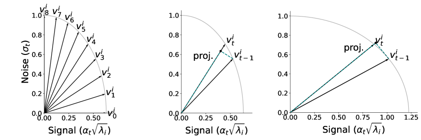
Figure 1: Geometric interpretation of the signal-noise vectors $\bm{v}_{t}^{i}=(\alpha_{t}\sqrt{\lambda_{i}},\sigma_{t})$, which lies on an ellipse. Equation˜7 corresponds to projecting $\bm{v}_{t-1}^{i}$ onto $\bm{v}_{t}^{i}$ and computing its ratio with $\|\bm{v}_{t}^{i}\|_{2}$. Left: full sequence of vectors ($T=8$). Middle: projection when $\lambda_{i}<1$. Right: projection when $\lambda_{i}>1$.

An important consequence of eq.˜8 is that the teacher cannot fully recover the original data distribution, even under perfect inference. This limitation arises from discretization error: approximating the continuous-time reverse process via a finite sequence of DDIM steps inherently introduces information loss. As a result, the composite operator contracts the variance of the signal. This phenomenon is formalized in proposition˜3.2, with proof given in appendix˜D.

Proposition 3.2 (Teacher model contracts the covariance).

Assume that the noise schedule $\{\alpha_{t}\}$ and $\{\sigma_{t}\}$ satisfies assumption˜2.1. Under the composite operator defined in eq.˜8, each output coordinate satisfies $(\mathcal{T}_{T}(\bm{z}_{T}))_{i}\leq\sqrt{\lambda_{i}}\cdot(\bm{z}_{T})_{i}$, with equality if and only if $(\bm{z}_{T})_{i}=0$. Consequently, if $\bm{z}_{T}\sim\mathcal{N}(\bm{0},\bm{I})$, then the teacher model defined in eq.˜10 produces samples with a contracted covariance matrix, i.e., $\mathrm{Cov}\bigl{(}\mathcal{T}_{T}(\bm{z}_{T})\bigr{)}\preceq\bm{\Lambda}$, where the inequality is strict if $\bm{\Lambda}\succ\bm{0}$.

3.2 Optimization dynamics of the student

Following corollary˜3.1, we use the parameterization $\bm{f}_{\bm{\eta}}$ in eq.˜3 and model both the teacher and student as time-dependent linear operators. The student model adopts the form

$$\bm{f}_{\text{st}}(\bm{z}_{t},t)=\bm{A}_{t}^{\text{st}}\bm{z}_{t},\quad\bm{A}_{t}^{\text{st}}=\mathrm{Diag}(a_{t}^{1},\dotsc,a_{t}^{d}),$$ (9)

with learnable diagonal weights. Following standard practice (Luhman and Luhman, 2021; Salimans and Ho, 2022), we initialize the student to match the single-step optimal operator (i.e., the teacher model),

$$\bm{A}_{t}^{\star}\coloneqq(\alpha_{t-1}\alpha_{t}\bm{\Lambda}+\sigma_{t-1}\sigma_{t}\bm{I})(\alpha_{t}^{2}\bm{\Lambda}+\sigma_{t}^{2}\bm{I})^{-1},$$ (10)

which corresponds to the optimal one-step DDIM update in corollary˜3.1. To train the student, we define a trajectory distillation loss in assumption˜3.2 that encourages the student to match the teacher’s behavior across multiple steps. Specifically, the loss at time $t$ measures the mean squared error between the student prediction and the multi-step composite operator output $\mathcal{T}_{k}(\bm{z}_{t})$.

Assumption 3.2 (Trajectory distillation loss).

Let $\bm{z}_{t}\sim p_{t}=(\alpha_{t}p_{0})*\mathcal{N}(\bm{0},\sigma_{t}^{2}\bm{I})$ be a noisy input at time $t$, and let the student model be defined by eq.˜9. We assume that the distillation loss at time $t$ is given by

$$\mathcal{L}_{t}(\bm{A}_{t}^{\text{st}})=\mathbb{E}_{\bm{z}_{t}\sim p_{t}}\left[\|\bm{A}_{t}^{\text{st}}\bm{z}_{t}-\mathcal{T}_{k}(\bm{z}_{t})\|_{2}^{2}\right].$$ (11)

For each coordinate $i$, let $a_{t}^{i}(s)$ denote the student’s value at training time $s$ (distinct from the diffusion time step $t$, which indexes the noise level). The student aims to approximate the $i$th entry of the composite operator, denoted $(\mathcal{T}_{k})_{i}$. The gradient flow of the distillation loss assumption˜3.2 leads to the following scalar ODE for each coordinate:

$$\frac{\mathrm{d}}{\mathrm{d}s}a_{t}^{i}(s)=-\nabla_{a_{t}^{i}}\mathcal{L}_{t}(\bm{A}_{t}^{\text{st}}),\quad a_{t}^{i}(0)=(\bm{A}_{t}^{\star})_{i}.$$ (12)

This ODE admits a closed-form solution, which is presented in proposition˜3.3, with the proof deferred to appendix˜E.

Proposition 3.3 (Student interpolation under gradient flow).

Let $\lambda_{i}$ be the $i$th diagonal entry of $\bm{\Lambda}$, and let $(\bm{A}_{t}^{\star})_{i}$ be the corresponding entry of the teacher operator. Under the gradient flow ODE in eq.˜12, the student update $a_{t}^{i}(s)$ evolves as

$$a_{t}^{i}(s)=(1-\gamma_{t}^{i}(s))\cdot(\mathcal{T}_{k})_{i}+\gamma_{t}^{i}(s)\cdot(\bm{A}_{t}^{\star})_{i},$$ (13)

where the interpolation weight $\gamma_{t}^{i}(s)=\exp\left(-2s\|\bm{v}_{t}^{i}\|_{2}^{2}\right)$, with $\bm{v}_{t}^{i}=(\alpha_{t}\sqrt{\lambda_{i}},\sigma_{t})^{\top}\in\mathbb{R}^{2}$ and $\|\bm{v}_{t}^{i}\|_{2}^{2}=\alpha_{t}^{2}\lambda_{i}+\sigma_{t}^{2}$.

Proposition˜3.3 reveals a fundamental limitation of trajectory distillation: under finite training time $s$, the student does not fully match the composite operator $(\mathcal{T}_{k})_{i}$, but instead interpolates between the multi-step target and the single-step teacher $(\bm{A}_{t}^{\star})_{i}$. The interpolation weight $\gamma_{t}^{i}(s)\in(0,1)$ depends exponentially on both $s$ and the signal-to-noise ratio $\|\bm{v}_{t}^{i}\|_{2}^{2}=\alpha_{t}^{2}\lambda_{i}+\sigma_{t}^{2}$, and quantifies the deviation from the target.

4 Optimal trajectory distillation via dynamic programming

In this section, we formalize trajectory distillation as an operator merging problem over a sequence of teacher operators, each corresponding to a single-step DDIM update. We introduce a recursive merge rule that models signal shrinkage via convex combinations, capturing the contraction effects induced by limited student optimization, as detailed in section˜4.1. To identify the optimal merging plan, we develop a dynamic programming algorithm that minimizes the Wasserstein-$2$ distance to a surrogate composite teacher, as presented in section˜4.2. Finally, we show that the optimal strategy exhibits a phase transition based on data variance, recovering canonical methods such as sequential BOOT and vanilla distillation in their respective regimes, as discussed in section˜4.3.

4.1 Operator merging problem under signal shrinkage

We formalize trajectory distillation as a sequential merging of teacher operators. Let $\bm{v}_{t}^{i}=(\alpha_{t}\sqrt{\lambda_{i}},\sigma_{t})^{\top}\in\mathbb{R}^{2}$ denote the signal-noise vector for coordinate $i$ at time $t$, as introduced in eq.˜7. Recall that the teacher operator updates the $i$th coordinate by

$$(\bm{z}_{t-1})_{i}=(\bm{A}_{t}^{\star})_{i}(\bm{z}_{t})_{i}=\frac{\langle\bm{v}_{t-1}^{i},\bm{v}_{t}^{i}\rangle}{\|\bm{v}_{t}^{i}\|_{2}^{2}}\cdot(\bm{z}_{t})_{i}.$$ (14)

We define the initial set of student operators at training step $k=0$, denoted with the superscript $(0)$, to match the teacher operator:

$$(\bm{A}_{t}^{(0)})_{i}\coloneqq(\bm{A}_{t}^{\star})_{i}=\frac{\langle\bm{v}_{t-1}^{i},\bm{v}_{t}^{i}\rangle}{\|\bm{v}_{t}^{i}\|_{2}^{2}},\quad t=1,\dots,T.$$ (15)

At each training step $k\geq 1$, the student may choose to merge a contiguous block of updates from $t=t_{1}+1$ to $t=t_{2}$, replacing $\bm{A}_{t_{1}+1}^{(k-1)},\dotsc,\bm{A}_{t_{2}}^{(k-1)}$ with a single merged operator $\bm{A}_{t_{1}+1:t_{2}}^{(k)}$, defined for each coordinate $i$ as

$$(\bm{A}_{t_{1}+1:t_{2}}^{(k)})_{i}=(1-\gamma_{t_{2}}^{i})\cdot\prod_{t=t_{1}+1}^{t_{2}}(\bm{A}_{t}^{(k-1)})_{i}+\gamma_{t_{2}}^{i}\cdot(\bm{A}_{t_{2}}^{(k-1)})_{i},$$ (16)

where the shrinkage factor is

$$\gamma_{t_{2}}^{i}=\exp(-2s\|\bm{v}_{t_{2}}^{i}\|_{2}^{2}),$$ (17)

and $s>0$ denotes the available optimization time, as derived in section˜3.2. This merging process is repeated until a complete trajectory $\bm{A}_{1:T}^{(K)}$ is constructed, where $K\geq 1$ denotes the total number of merge operations. The resulting operator defines the student’s final sampling function: when applied to a standard Gaussian input $\bm{z}_{T}\sim\mathcal{N}(\bm{0},\bm{I})$, it produces the output distribution of the student model.

The quality of the merged trajectory is evaluated using the squared Wasserstein-$2$ distance between the student’s output distribution and that of a surrogate target $\widetilde{\mathcal{T}}_{T}$, which approximates the ideal composite behavior. Specifically, we define $\widetilde{\mathcal{T}}_{T}$ coordinate-wise by suppressing subunit contractions when $\lambda_{i}>1$, as formalized in definition˜4.1.

Definition 4.1 (Surrogate composite operator).

Let $\widetilde{\mathcal{T}}_{T}$ be a modified composite operator defined coordinate-wise as follows. For each $i\in\{1,\dotsc,d\}$, define:

$$(\widetilde{\mathcal{T}}_{T})_{i}=\prod_{t=1}^{T}(\widetilde{\bm{A}}_{t}^{\star})_{i},\quad\text{where}\quad(\widetilde{\bm{A}}_{t}^{\star})_{i}\coloneqq\begin{cases}(\bm{A}_{t}^{\star})_{i},&\text{if }\lambda_{i}\leq 1\text{ or }(\bm{A}_{t}^{\star})_{i}\geq 1,\\ 1,&\text{if }\lambda_{i}>1\text{ and }(\bm{A}_{t}^{\star})_{i}<1.\end{cases}$$ (18)

For each coordinate $i$, we define the discrepancy $\delta_{i}\coloneqq\bigl{(}(\widetilde{\mathcal{T}}_{T})_{i}-(\bm{A}_{1:T}^{(K)})_{i}\bigr{)}^{2}$, which captures the squared Wasserstein-$2$ distance between the marginal distributions along dimension $i$. The overall squared Wasserstein-$2$ distance is given by $\mathcal{L}_{W_{2}}\coloneqq\sum_{i=1}^{d}\delta_{i}$. This reframes trajectory distillation as a merge planning problem, where the goal is to approximate $\widetilde{\mathcal{T}}_{T}$ as closely as possible while reducing the number of merged operators to one.

4.2 Optimal operator merging via dynamic programming

Algorithm 1 Optimal trajectory merge via dynamic programming

1:Single-step teacher operators $\{\bm{A}_{t}^{\star}\}_{t=1}^{T}$, shrinkage matrices $\{\bm{\Gamma}_{t}=\mathrm{Diag}(\gamma_{t}^{1},\dotsc,\gamma_{t}^{d})\}_{t=1}^{T}$, surrogate composite operator $\widetilde{\mathcal{T}}_{T}$

2:for $t=1$ to $T$ do

3:  $\texttt{dp}[t][t]\leftarrow\bm{A}_{t}^{\star}$ $\triangleright$ Base case: no merge needed for length-$1$ blocks

4:end for

5:for $\ell=2$ to $T$ do $\triangleright$ Iterate over all block lengths

6:  for $t_{1}=1$ to $T-\ell+1$ do

7:    $t_{2}\leftarrow t_{1}+\ell-1$

8:    $\text{best\_error}\leftarrow\infty$ $\triangleright$ Option 1: directly merge all operators in $[t_{1}+1,t_{2}]$

9:    $\bm{A}_{t_{1}+1:t_{2}}^{\text{direct}}\leftarrow(\bm{I}-\bm{\Gamma}_{t_{2}})\cdot\prod_{t=t_{1}+1}^{t_{2}}\bm{A}_{t}^{\star}+\bm{\Gamma}_{t_{2}}\cdot\bm{A}_{t_{2}}^{\star}$

10:    $\text{error}\leftarrow\sum_{i}\bigl{(}(\widetilde{\mathcal{T}}_{T})_{i}-(\bm{A}_{t_{1}+1:t_{2}}^{\text{direct}})_{i}\bigr{)}^{2}$

11:    $\texttt{dp}[t_{1}][t_{2}]\leftarrow\bm{A}_{t_{1}+1:t_{2}}^{\text{direct}}$ $\triangleright$ Option 2: try all valid binary splits of $[t_{1}+1,t_{2}]$

12:    for $m=t_{1}+1$ to $t_{2}-1$ do

13:     $\bm{A}_{t_{1}+1:m}\leftarrow\texttt{dp}[t_{1}][m]$, $\bm{A}_{m+1:t_{2}}\leftarrow\texttt{dp}[m+1][t_{2}]$

14:     $\bm{A}_{t_{1}+1:t_{2}}^{\text{split}}\leftarrow(\bm{I}-\Gamma_{t_{2}})\cdot\bm{A}_{t_{1}+1:m}\cdot\bm{A}_{m+1:t_{2}}+\Gamma_{t_{2}}\cdot\bm{A}_{m+1:t_{2}}$

15:     $\text{error}\leftarrow\sum_{i}\bigl{(}(\widetilde{\mathcal{T}}_{T})_{i}-(\bm{A}_{t_{1}+1:t_{2}}^{\text{split}})_{i}\bigr{)}^{2}$

16:     if $\text{error}<\text{best\_error}$ then

17:      $\texttt{dp}[t_{1}][t_{2}]\leftarrow\bm{A}_{t_{1}+1:t_{2}}^{\text{split}}$ $\triangleright$ Update best merge for this block

18:      $\text{best\_error}\leftarrow\text{error}$

19:     end if

20:    end for

21:  end for

22:end for

23:return $\texttt{dp}[1][T]$ $\triangleright$ Final merged operator over full trajectory

To address the operator merging problem formulated in section˜4.1, we employ a dynamic programming approach. Given the single-step teacher operators $\{\bm{A}_{t}^{(0)}\}_{t=1}^{T}$ (for simplicity, we omit the superscript in what follows), the goal is to construct a merged operator $\bm{A}_{1:T}$ that best approximates the surrogate composite teacher operator $\widetilde{\mathcal{T}}_{T}$ defined in definition˜4.1, by minimizing the squared discrepancy

$$\mathcal{L}_{W_{2}}=\sum_{i=1}^{d}\bigl{(}(\widetilde{\mathcal{T}}_{T})_{i}-(\bm{A}_{1:T})_{i}\bigr{)}^{2}.$$ (19)

We define the merged operator over an interval $[t_{1}+1,t_{2}]$ recursively. For each coordinate $i$, the merged value $(\bm{A}_{t_{1}+1:t_{2}})_{i}$ can be obtained in one of two ways: (i) direct merge, which multiply all single-step operators in the interval, then apply shrinkage due to limited optimization:

$$(\bm{A}_{t_{1}+1:t_{2}}^{\text{direct}})_{i}=(1-\gamma_{t_{2}}^{i})\cdot\prod_{t=t_{1}+1}^{t_{2}}(\bm{A}_{t})_{i}+\gamma_{t_{2}}^{i}\cdot(\bm{A}_{t_{2}})_{i}.$$ (20)

Alternatively (ii) choose a midpoint $m\in\{t_{1}+1,\dotsc,t_{2}-1\}$, recursively merge the two subintervals, and apply shrinkage:

$$(\bm{A}_{t_{1}+1:t_{2}}^{\mathrm{split}})_{i}=(1-\gamma_{t_{2}}^{i})\cdot(\bm{A}_{t_{1}+1:m})_{i}\cdot(\bm{A}_{m+1:t_{2}})_{i}+\gamma_{t_{2}}^{i}\cdot(\bm{A}_{m+1:t_{2}})_{i}.$$ (21)

For each candidate merge over the interval $[t_{1}+1,t_{2}]$, we measure its quality via the coordinate-wise discrepancy:

$$\mathcal{L}_{W_{2}}^{t_{1}+1:t_{2}}\coloneqq\sum_{i=1}^{d}\bigl{(}(\widetilde{\mathcal{T}}_{T})_{i}-(\bm{A}_{t_{1}+1:t_{2}}^{\text{candidate}})_{i}\bigr{)}^{2},\quad\text{candidate}\in\{\text{direct},\text{split}\}.$$ (22)

The dynamic programming algorithm computes the optimal merge for each interval $[t_{1}+1,t_{2}]$, in order of increasing length. For each interval, we compare the error of direct merging with all possible binary splits, and store the merge plan that minimizes discrepancy. This yields the minimal-discrepancy merge plan over the entire trajectory. The full procedure is summarized in algorithm˜1. While $\widetilde{\mathcal{T}}_{T}$ is not the true composite operator of the teacher model, it serves as a surrogate that enables tractable analysis while preserving the necessary structure. In particular, it ensures that any suboptimal merge decision leads to a provable increase in the Wasserstein-$2$ discrepancy. We now show in theorem˜4.1 that under this surrogate loss, the dynamic programming algorithm yields a globally optimal merge plan. Its proof is deferred to appendix˜F.

Theorem 4.1 (Optimality of dynamic programming merge).

The dynamic programming algorithm in algorithm˜1, when applied to single-step operators $\{\bm{A}_{t}^{\star}\}_{t=1}^{T}$ with fixed shrinkage matrices $\{\bm{\Gamma}_{t}\}_{t=1}^{T}$, returns the merged operator $\bm{A}_{1:T}$ that globally minimizes $\mathcal{L}_{W_{2}}$ over all valid recursive merge plans.

4.3 Optimal strategy coincides with canonical strategies in specific regimes

In this section, we investigate how the optimal merge strategy depends on the covariance matrix $\bm{\Lambda}$, revealing a sharp phase transition. We characterize this transition between two regimes: (i) when $\lambda\leq 1$, the optimal merge strategy follows sequential BOOT; (ii) for large $\lambda$, it reduces to vanilla trajectory distillation. We focus on the scalar case ($d=1$), where $\bm{\Lambda}=\lambda$, and omit the superscript $i$ and subscript $i$ in $\gamma_{t}^{i}$ and $(\bm{A}_{t})_{i}$, respectively. We also use the non-bold form $A_{t}$ instead of $\bm{A}_{t}$ to distinguish it from matrix notation.

When $\lambda\gg 1$, the optimal merge strategy is to perform a one-shot merge over all denoising steps, corresponding to the vanilla trajectory distillation. In this regime, the intermediate single-step operators $A_{t}^{\star}$ satisfy $A_{t}^{\star}>1$ for $t<T$, meaning that each step amplifies the signal. Merging these steps early helps preserve this amplification. The final step $A_{T}^{\star}<1$ introduces a small contraction, but this effect is minimal when preceded by strong signal gains. We formally establish the optimality of vanilla trajectory distillation in theorem˜4.2, with the complete proof provided in appendix˜G.

Theorem 4.2 (Vanilla trajectory distillation is optimal when $\lambda\gg 1$).

Consider the surrogate optimization problem described in section˜4.2 in the scalar setting, and assume $\bm{\Lambda}=\lambda\gg 1$. Then, for the sequence of single-step updates $\{A_{1}^{\star},A_{2}^{\star},\dotsc,A_{T}^{\star}\}$ in eq.˜15, the optimal merge strategy that minimizes the squared error to the surrogate target $\prod_{t=1}^{T}\widetilde{A}_{t}^{\star}$ is the vanilla trajectory distillation: all steps are merged in a single one-shot update without intermediate composition.

In contrast, when $\lambda\leq 1$, all operators satisfy $A_{t}^{\star}\leq 1$, and the trajectory contracts monotonically. In this regime, the best approach is to merge steps gradually in a reverse order, starting from the highest noise level. This corresponds to the sequential BOOT strategy, where the student is trained to merge $\{A_{T}^{\star},A_{T-1}^{\star}\}$, then merges the result with $A_{T-2}^{\star}$, and so on. This strategy minimizes compounding error by ensuring that each merge occurs over a shorter horizon with limited shrinkage. The following theorem˜4.3 establishes the optimality of this strategy, with the proof given in appendix˜H.

Theorem 4.3 (Sequential BOOT is optimal when $\lambda\leq 1$).

Consider the surrogate optimization problem described in section˜4.2 in the scalar setting, and assume $\bm{\Lambda}=\lambda\leq 1$. Then, for the sequence of single-step updates $\{A_{1}^{\star},A_{2}^{\star},\dotsc,A_{T}^{\star}\}$ in eq.˜15, the optimal merge strategy that minimizes the squared error to the surrogate target $\prod_{t=1}^{T}A_{t}^{\star}$ (which coincides with the original composite operator when $\lambda\leq 1$) is the sequential BOOT merge: starting from $A_{T}^{\star}$, iteratively merge it with $A_{T-1}^{\star}$, then with $A_{T-2}^{\star}$, and so on, until all steps are merged into a single operator.

5 Experiments

In this section, we present experimental results to validate our theoretical findings. We begin by evaluating algorithm˜1 for optimal trajectory merging, as discussed in section˜5.1. Then, in section˜5.2, we provide simulation results using synthetic datasets. The experimental details and addition results on real dataset are provided in appendices˜I, J and K.

5.1 Dynamic programming results

We implement the dynamic programming algorithm described in algorithm˜1. For visualization purposes, we set the total number of time steps to $T=32$ and the student’s training time per merge step to $s=6.4$. Throughout our experiments, we adopt the cosine noise schedule, defined by $\alpha_{t}=\cos((t/T)\cdot\pi/2)$ and $\sigma_{t}=\sin((t/T)\cdot\pi/2)$, which is commonly used in prior works (Nichol and Dhariwal, 2021). The results, showing the error gap between four canonical strategies and the DP-optimal solution, are presented in the first row of fig.˜2. As predicted by theorem˜4.2 and theorem˜4.3, when $\lambda\leq 1$, sequential BOOT achieves optimality (with zero error gap). As $\lambda$ increases beyond $2$, vanilla trajectory distillation becomes the optimal strategy. In the transitional regime between these extremes, the optimal merge plan exhibits a hybrid structure: in particular, parts of the merge path may align with sequential consistency (especially when $\lambda$ is close to $1$), but the overall pattern deviates from any previously known strategy. We visualize two representative cases at $\lambda=1.08$ and $\lambda=2$ in the second row of fig.˜2, where each arc denotes a merge operation and the arc color encodes the merge order. Lighter colors indicate earlier merges, while darker colors correspond to later ones. Finally, for ablation studies under varying $T$, $s$, and covariance matrices $\bm{\Lambda}$, please refer to appendix˜I.

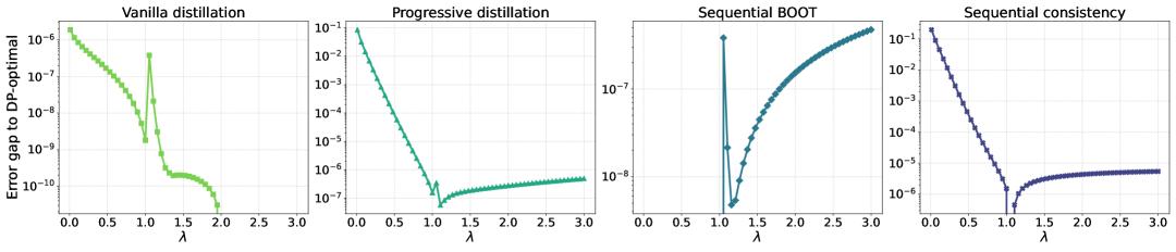
Figure 2: First row: Error gap between four canonical strategies and the DP-optimal solution as a function of $\lambda$, with $T=32$ and $s=6.4$. As predicted by theorem˜4.2 and theorem˜4.3, sequential BOOT achieves optimality when $\lambda\leq 1$, while vanilla trajectory distillation becomes optimal for sufficiently large $\lambda>2$. Second row: Visualization of the DP-optimal merge plans at $\lambda=1.08$ (left) and $\lambda=2$ (right). Each arc represents a merge operation, with lighter colors indicating earlier merges and darker colors corresponding to later merges. For additional results under varying $T$, $s$, and covariance matrices $\bm{\Lambda}$, please refer to appendix˜I.

5.2 Experiments on synthetic datasets

In table˜2, we present results from experiments on synthetic datasets to evaluate the effectiveness of different trajectory distillation strategies. Specifically, we vary the covariance parameter $\lambda$ and compare the performance of four canonical methods. The evaluation metric is the average Wasserstein-$2$ distance error, computed over $10$ independent trials. For each $\lambda$, the best-performing method is underlined. The observed trends are consistent with theoretical predictions derived from our analysis in the linear regime. For additional experimental results please refer to appendix˜J.

Table 2: Simulation results of four canonical trajectory distillation methods on synthetic datasets with varying covariance parameter $\lambda$. Each entry reports the mean signed error between the student operator and the surrogate composite operator, averaged over $10$ independent trials. Error bars represent standard deviation across trials. The best result for each setting is underlined. Results are consistent with our theoretical predictions.

$\lambda$	Vanilla	Progressive	BOOT	Consistency
0.20	$7.3\times 10^{-4}\pm 1.3\times 10^{-4}$	$3.3\times 10^{-2}\pm 5.2\times 10^{-4}$	$\underline{4.7\times 10^{-4}}\pm 7.1\times 10^{-5}$	$1.3\times 10^{-1}\pm 7.8\times 10^{-3}$
0.50	$4.5\times 10^{-4}\pm 9.4\times 10^{-5}$	$4.8\times 10^{-3}\pm 1.1\times 10^{-4}$	$\underline{3.9\times 10^{-4}}\pm 6.1\times 10^{-5}$	$2.6\times 10^{-2}\pm 2.3\times 10^{-3}$
1.00	$\underline{4.7\times 10^{-5}}\pm 6.4\times 10^{-6}$	$1.3\times 10^{-4}\pm 9.1\times 10^{-6}$	$5.3\times 10^{-5}\pm 7.0\times 10^{-6}$	$-1.2\times 10^{-4}\pm 1.1\times 10^{-4}$
1.02	$-2.8\times 10^{-2}\pm 5.3\times 10^{-6}$	$\underline{-2.8\times 10^{-2}}\pm 5.5\times 10^{-6}$	$-2.8\times 10^{-2}\pm 3.8\times 10^{-6}$	$-2.9\times 10^{-2}\pm 1.1\times 10^{-4}$
2.00	$\underline{-2.1\times 10^{-3}}\pm 6.2\times 10^{-5}$	$-2.4\times 10^{-3}\pm 7.1\times 10^{-5}$	$-2.2\times 10^{-3}\pm 1.1\times 10^{-4}$	$-7.1\times 10^{-3}\pm 6.9\times 10^{-4}$
5.00	$\underline{-4.1\times 10^{-3}}\pm 3.7\times 10^{-4}$	$-4.7\times 10^{-3}\pm 1.7\times 10^{-4}$	$-4.9\times 10^{-3}\pm 4.8\times 10^{-4}$	$-1.1\times 10^{-2}\pm 8.3\times 10^{-4}$

6 Conclusion

We analyzed diffusion trajectory distillation as an operator merging problem in the linear regime, providing theoretical insights into optimal strategies via dynamic programming. Our analysis uncovers a phase transition between canonical distillation methods, governed by the data variance: sequential BOOT is optimal when variances are small, vanilla distillation dominates when variances are large, and intricate merge structures emerge in the transitional regime. These findings establish a unified perspective for understanding, comparing, and designing distillation strategies grounded in signal fidelity and compression trade-offs.

While our analysis relies on simplifying assumptions such as a Gaussian data distribution and fixed optimization time per merge step, these are well-supported both theoretically and practically. Diffusion models exhibit an inductive bias toward Gaussian-like structures under limited capacity, and computational constraints naturally impose fixed optimization budgets in practice.

Looking ahead, promising directions include generalizing the analysis to multimodal data (e.g., via Gaussian mixtures), incorporating intermediate-step student models, and integrating stabilization techniques such as Exponential Moving Average (EMA) and timestep mixing. Importantly, our results highlight that optimal merge planning is not merely a training heuristic but a central design axis in diffusion distillation. We hope this perspective offers a foundation for more principled and generalizable algorithms in future work. See appendix˜L for extended discussion.

Roadmap.

The appendix is organized as follows:

• Appendix˜A provides an additional literature review.

• Appendix˜B details the four canonical trajectory distillation methods, complementing table˜1.

• Appendix˜C presents the proof of proposition˜3.1 ( (Optimal denoising estimator is linear).).

• Appendix˜D presents the proof of proposition˜3.2 ( (Teacher model contracts the covariance).).

• Appendix˜E presents the proof of proposition˜3.3 ( (Student interpolation under gradient flow).).

• Appendix˜F provides the proof of theorem˜4.1 ( (Optimality of dynamic programming merge).).

• Appendix˜G presents the proof of theorem˜4.2 ( (Vanilla trajectory distillation is optimal when $\lambda\gg 1$).).

• Appendix˜H presents the proof of theorem˜4.3 ( (Sequential BOOT is optimal when $\lambda\leq 1$).).

• Appendix˜I presents extended results on dynamic programming, complementing section˜5.1.

• Appendix˜J provides further experiments on synthetic datasets, complementing section˜5.2.

• Appendix˜K reports experimental results on a real dataset.

• Appendix˜L discusses assumptions, practical considerations, and potential extensions not covered in the main text.

Appendix A Additional literature review

Diffusion models [Ho et al., 2020, Karras et al., 2022, Nichol and Dhariwal, 2021, Ren et al., 2025, Song et al., 2021a, Song and Ermon, 2019, Song et al., 2021b] have emerged as a powerful class of generative models that generate samples by denoising a random Gaussian input through a sequence of learned transformations. Their strength lies in the use of a multi-step refinement process, which gradually improves the fidelity and realism of generated samples. This iterative nature enables fine control over the generative process and contributes to the impressive sample quality observed in recent models [Ramesh et al., 2022, Rombach et al., 2022, Saharia et al., 2022]. However, this comes at the cost of slow inference: generating a single image typically requires hundreds or even thousands of denoising steps.

To address this bottleneck, various acceleration techniques have been proposed. One prominent direction is to reinterpret diffusion as a continuous-time process [Song et al., 2021b] and apply advanced ODE/SDE solvers to reduce the number of required steps [Karras et al., 2022, Liu et al., 2022, Lu et al., 2022a, b, Zhao et al., 2023]. These approaches, known as fast samplers or solver-based methods, can reduce inference time to $20$–$50$ steps while maintaining high sample quality. Despite these advances, the performance gap between accelerated sampling and full-length diffusion remains significant, especially under extremely low-step regimes. Parallel to this work, research on optimizing sampling schedules and step sizes [Nguyen et al., 2024, Pei et al., 2025] has also emerged. This line of work focuses on balancing sampling speed and generative quality, but approaches the problem from a training-based perspective, rather than relying on solvers.

An alternative and increasingly popular strategy is diffusion distillation [Berthelot et al., 2023, Gu et al., 2023, Li et al., 2024a, Lin et al., 2024, Luhman and Luhman, 2021, Luo et al., 2023, Meng et al., 2023, Salimans and Ho, 2022, Sauer et al., 2024, Song et al., 2024, Xu et al., 2025, Yin et al., 2024a, b, Zhou et al., 2025, 2024], which aims to train a student model that approximates the behavior of a pre-trained teacher model in fewer steps. Among distillation methods, we identify three main families: diffusion trajectory distillation, distribution matching distillation, and adversarial distillation.

Diffusion trajectory distillation.

These methods accelerate diffusion sampling by compressing the teacher’s denoising trajectory into a shorter sequence of student updates. The term trajectory refers to the sequence of intermediate states generated by the reverse process, which the student aims to reproduce by merging multiple teacher steps into one. This includes vanilla distillation [Luhman and Luhman, 2021], which learns a one-step approximation of the full trajectory; progressive distillation [Lin et al., 2024, Meng et al., 2023, Salimans and Ho, 2022], which halves the number of steps iteratively; consistency models [Li et al., 2024a, Song et al., 2024], which aim to map noisy samples at arbitrary timesteps to a shared clean target via a consistency objective; and BOOT [Gu et al., 2023], which maps the noisiest sample step-by-step to lower-noise states by matching the student to single-step teacher outputs. These methods rely on explicit supervision from a high-quality teacher and can reduce inference to under $10$ steps with minimal quality loss.

Distribution matching distillation.

Rather than imitating the teacher’s trajectory step-by-step, these methods aim to match the probability distributions induced by the student and teacher models at various noise levels. The underlying principle is to minimize a divergence between the two distributions, such as the Kullback–Leibler divergence [Yin et al., 2024a, b], Fisher divergence [Zhou et al., 2024], $f$-divergence [Xu et al., 2025], or integral probability metrics like the integral KL [Luo et al., 2023]. This typically requires training an auxiliary student score network to approximate the gradient of the log-density. While this approach offers greater flexibility, it is often more challenging to train in practice. Many methods rely on trajectory distillation to stabilize training [Yin et al., 2024b].

Adversarial distillation.

This family of methods trains the student using adversarial objectives to match the real data distribution, potentially allowing the student to outperform the teacher and overcome its limitations [Sauer et al., 2024]. To this end, an auxiliary discriminator is trained to distinguish real samples from those generated by the student at different noise levels. However, this discrimination task becomes increasingly difficult at high noise levels, where both real and generated samples are heavily corrupted. As a result, adversarial distillation often requires careful discriminator design and training stabilization. In practice, it is typically combined with trajectory distillation [Lin et al., 2024] or distribution matching distillation [Yin et al., 2024a, Zhou et al., 2025] to improve robustness and overall performance.

Despite the rapid empirical advancements in diffusion distillation, many of these methods remain theoretically underexplored. While Xu et al. [2024] provides preliminary insights by demonstrating that partitioning the diffusion process into smaller intervals reduces the distribution gap between sub-models, enabling faster training and inference, the impact of different trajectory merging strategies on the quality of the student model is still not well understood. Additionally, how optimization constraints, such as limited training time, interact with the reverse process structure remains unclear. This theoretical gap has led to the development of many heuristic methods, often without a clear understanding of why or when they are effective.

In this work, we take a step toward a principled understanding by focusing on diffusion trajectory distillation, a subclass of methods in which the student model is trained to directly imitate a sequence of teacher denoising steps. Unlike distribution-matching or adversarial approaches, trajectory distillation relies solely on the teacher model for supervision and does not require auxiliary components such as a student score network or discriminator. This structural simplicity enables theoretical analysis by eliminating the complications introduced by learned gradients or adversarial dynamics. Within this setting, we study the mechanics of trajectory merging in a linear regime, reveal the implicit shrinkage effects introduced by discretization and optimization, and develop a dynamic programming algorithm to identify the optimal merge strategy. Our analysis helps explain the empirical success of methods like BOOT and vanilla distillation, and provides a unified perspective for understanding and improving diffusion distillation.

Appendix B Introduction to diffusion trajectory distillation methods

Trajectory distillation accelerates sampling by training a student model to approximate a composite operator $\mathcal{T}_{k}(\bm{z}_{t})$ as defined in definition˜2.1. We describe four canonical methods, including two widely adopted baselines and two sequential variants we design.

Vanilla distillation.

Originally proposed by Luhman and Luhman [2021], vanilla distillation trains a student model $\bm{A}_{\bm{\phi}}$ to match the entire teacher trajectory in a single forward pass:

$$\bm{A}_{\bm{\phi}}(\bm{z}_{T},T)\approx\mathcal{T}_{T}(\bm{z}_{T})=\bm{z}_{0}.$$ (23)

The goal is to learn a one-step mapping that directly transforms the noisy input $\bm{z}_{T}$ into a clean sample $\bm{z}_{0}$. See fig.˜3 for a conceptual illustration. While efficient during inference, this approach requires the student to capture a highly complex transformation, which can be challenging in practice.

Figure 3: Conceptual illustration of vanilla distillation. The entire teacher trajectory is being merged into a single step.

Progressive distillation.

Progressive distillation [Lin et al., 2024, Meng et al., 2023, Salimans and Ho, 2022] adopts a curriculum of merging two teacher steps at a time. In each round, the student model $\bm{A}_{\bm{\phi}}$ is trained to approximate

$$\bm{A}_{\bm{\phi}}(\bm{z}_{t},t)\approx\mathcal{T}_{2}(\bm{z}_{t})=\bm{z}_{t-2}$$ (24)

for even-indexed timesteps $t$. See fig.˜4 for a conceptual illustration. Once trained, the student replaces the teacher, and the number of sampling steps is halved. This procedure is repeated until only one step remains. The progressive reduction of the trajectory length eases optimization by distributing the learning burden over multiple stages.

Figure 4: Conceptual illustration of progressive distillation. The student model is trained with a curriculum that progressively merges pairs of teacher steps into a single student update, thereby halving the number of sampling steps required at each stage.

Sequential consistency.

The standard form of consistency distillation [Li et al., 2024a, Song et al., 2024] trains a student $\bm{A}_{\bm{\phi}}$ to satisfy the self-consistency condition

$$\bm{A}_{\bm{\phi}}(\bm{z}_{t},t)\approx\bm{A}_{\bm{\phi}}(\bm{z}_{t-1},t-1),$$ (25)

enforcing that all intermediate predictions follow a consistent trajectory toward the data distribution endpoint. We propose a sequential variant that adopts a curriculum strategy: the student model is explicitly trained to map each $\bm{z}_{t}$ directly to the clean sample $\bm{x}_{0}=\bm{z}_{0}$, using increasingly long trajectories. Formally, we train

$$\bm{A}_{\bm{\phi}}(\bm{z}_{t},t)\approx\mathcal{T}_{t}(\bm{z}_{t})=\bm{z}_{0},$$ (26)

for $t=1,2,\dotsc,T$. See fig.˜5 for a conceptual illustration. The student thus progressively learns to compress longer denoising trajectories into a single step, with early training focusing on short and easier sub-trajectories.

Figure 5: Conceptual illustration of sequential consistency distillation. The student model is trained to map each $\bm{z}_{t}$ directly to the clean sample $\bm{z}_{0}$, progressively learning to compress longer teacher trajectories into a single step.

Sequential BOOT.

BOOT [Gu et al., 2023] is a bootstrapping-based method that predicts the output of a pre-trained diffusion model teacher given any time-step, i.e.,

$$\bm{A}_{\bm{\phi}}(\bm{z}_{T},t)\approx\bm{z}_{t},\quad\bm{z}_{T}\sim\mathcal{N}(\bm{0},\bm{I})$$ (27)

Our sequential variant modifies this idea by keeping the input fixed at the noisiest level $\bm{z}_{T}$, while gradually shifting the target toward cleaner samples. Specifically, the student is trained to match

$$\bm{A}_{\bm{\phi}}(\bm{z}_{T},T)\approx\mathcal{T}_{k}(\bm{z}_{T})=\bm{z}_{T-k},$$ (28)

with $k=1,2,\dotsc,T$. See fig.˜6 for a conceptual illustration. This formulation constructs a monotonic training trajectory from high to low noise levels, offering a smooth learning process.

Figure 6: Conceptual illustration of sequential BOOT distillation. The student model is trained with input fixed at the noisiest level $\bm{z}_{T}$, while the target is gradually shifted toward cleaner samples.

Appendix C Optimal denoising estimator

See 3.1

Proof.

We prove a more general result: suppose $\bm{x}_{0}\sim\mathcal{N}(\bm{\mu},\bm{\Sigma})$, and the forward process is defined by

$$\bm{z}_{t}=\alpha_{t}\bm{x}_{0}+\sigma_{t}\bm{\epsilon},\quad\bm{\epsilon}\sim\mathcal{N}(\bm{0},\bm{I}).$$ (29)

Then the conditional distribution $p(\bm{x}_{0}|\bm{z}_{t})$ is Gaussian, and the optimal estimator minimizing squared error is its conditional expectation:

$$\mathbb{E}[\bm{x}_{0}|\bm{z}_{t}]=\bm{A}_{t}\bm{z}_{t}+\bm{b}_{t},$$ (30)

where

$$\bm{A}_{t}=\alpha_{t}\bm{\Sigma}(\alpha_{t}^{2}\bm{\Sigma}+\sigma_{t}^{2}\bm{I})^{-1},\quad\bm{b}_{t}=(\bm{I}-\alpha_{t}\bm{A}_{t})\bm{\mu}.$$ (31)

To derive this, we note that $\bm{z}_{t}|\bm{x}_{0}\sim\mathcal{N}(\alpha_{t}\bm{x}_{0},\sigma_{t}^{2}\bm{I})$, and hence the joint distribution is

$$\begin{bmatrix}\bm{x}_{0}\\ \bm{z}_{t}\end{bmatrix}\sim\mathcal{N}\biggl{(}\begin{bmatrix}\bm{\mu}\\ \alpha_{t}\bm{\mu}\end{bmatrix},\begin{bmatrix}\bm{\Sigma}&\alpha_{t}\bm{\Sigma}\\ \alpha_{t}\bm{\Sigma}&\alpha_{t}^{2}\bm{\Sigma}+\sigma_{t}^{2}\bm{I}\end{bmatrix}\biggr{)}.$$ (32)

The conditional mean is given by the standard Gaussian conditioning formula:

$$\mathbb{E}[\bm{x}_{0}|\bm{z}_{t}]=\bm{\mu}+\alpha_{t}\bm{\Sigma}(\alpha_{t}^{2}\bm{\Sigma}+\sigma_{t}^{2}\bm{I})^{-1}(\bm{z}_{t}-\alpha_{t}\bm{\mu}).$$ (33)

Rewriting this as an affine function of $\bm{z}_{t}$, we obtain

$$\mathbb{E}[\bm{x}_{0}|\bm{z}_{t}]=\underbrace{\alpha_{t}\bm{\Sigma}(\alpha_{t}^{2}\bm{\Sigma}+\sigma_{t}^{2}\bm{I})^{-1}}_{\bm{A}_{t}}\bm{z}_{t}+\underbrace{(\bm{I}-\alpha_{t}\bm{A}_{t})\bm{\mu}}_{\bm{b}_{t}}.$$ (34)

Now consider the case where $\bm{\mu}=\bm{0}$ and $\bm{\Sigma}$ is diagonal. More generally, suppose $\bm{\Sigma}=\bm{U}\bm{\Lambda}\bm{U}^{\top}$ is the eigendecomposition of the covariance. Then

$$\bm{A}_{t}=\alpha_{t}\bm{U}\bm{\Lambda}(\alpha_{t}^{2}\bm{\Lambda}+\sigma_{t}^{2}\bm{I})^{-1}\bm{U}^{\top},$$ (35)

so the estimator becomes

$$\mathbb{E}[\bm{x}_{0}|\bm{z}_{t}]=\bm{U}\bigl{(}\alpha_{t}\bm{\Lambda}(\alpha_{t}^{2}\bm{\Lambda}+\sigma_{t}^{2}\bm{I})^{-1}\bigr{)}\bm{U}^{\top}\bm{z}_{t}.$$ (36)

In particular, if $\bm{\Sigma}=\bm{\Lambda}$ is diagonal, then $\bm{U}=\bm{I}$, and we recover the expression in the proposition:

$$\mathbb{E}[\bm{x}_{0}|\bm{z}_{t}]=\alpha_{t}\bm{\Lambda}(\alpha_{t}^{2}\bm{\Lambda}+\sigma_{t}^{2}\bm{I})^{-1}\bm{z}_{t}.$$ (37)

This completes the proof. ∎

Appendix D Teacher model contracts the covariance

See 3.2

Proof.

Fix a coordinate $i$, and consider the evolution of the $i$th component in the DDIM process. From eq.˜8, we know that the teacher applies the operator

$$(\mathcal{T}_{T}(\bm{z}_{T}))_{i}=\biggl{(}\prod_{t=1}^{T}\frac{\langle\bm{v}_{t-1}^{i},\bm{v}_{t}^{i}\rangle}{\|\bm{v}_{t}^{i}\|_{2}^{2}}\biggr{)}\cdot(\bm{z}_{T})_{i},$$ (38)

where $\bm{v}_{t}^{i}=(\alpha_{t}\sqrt{\lambda_{i}},\sigma_{t})^{\top}\in\mathbb{R}^{2}$ is the signal-noise vector defined in eq.˜8. By the Cauchy–Schwarz inequality, we have for all $i$:

$$\frac{\langle\bm{v}_{t-1}^{i},\bm{v}_{t}^{i}\rangle}{\|\bm{v}_{t}^{i}\|_{2}^{2}}\leq\frac{\|\bm{v}_{t-1}^{i}\|_{2}\cdot\|\bm{v}_{t}^{i}\|_{2}}{\|\bm{v}_{t}^{i}\|_{2}^{2}}=\frac{\|\bm{v}_{t-1}^{i}\|_{2}}{\|\bm{v}_{t}^{i}\|_{2}}.$$ (39)

Taking the product from $t=1$ to $T$, we obtain

$$\prod_{t=1}^{T}\frac{\langle\bm{v}_{t-1}^{i},\bm{v}_{t}^{i}\rangle}{\|\bm{v}_{t}^{i}\|_{2}^{2}}\leq\prod_{t=1}^{T}\frac{\|\bm{v}_{t-1}^{i}\|_{2}}{\|\bm{v}_{t}^{i}\|_{2}}=\frac{\|\bm{v}_{0}^{i}\|_{2}}{\|\bm{v}_{T}^{i}\|_{2}}.$$ (40)

Using the boundary conditions $\alpha_{0}=1$, $\sigma_{0}=0$, $\alpha_{T}=0$, and $\sigma_{T}=1$, we find

$$\|\bm{v}_{0}^{i}\|_{2}=\sqrt{\lambda_{i}},\quad\|\bm{v}_{T}^{i}\|_{2}=1,$$ (41)

which implies

$$(\mathcal{T}_{T}(\bm{z}_{T}))_{i}\leq\sqrt{\lambda_{i}}\cdot(\bm{z}_{T})_{i}.$$ (42)

Equality holds if and only if equality holds in the Cauchy–Schwarz inequality at each step, which occurs if and only if all vectors $\bm{v}_{j-1}^{i}$ and $\bm{v}_{j}^{i}$ are positively collinear. Since the signal-noise vectors vary across time steps due to the schedule $(\alpha_{t},\sigma_{t})$, this happens only when the projection scalar acts on zero input, i.e., $(\bm{z}_{T})_{i}=0$.

Now assume $\bm{z}_{T}\sim\mathcal{N}(\bm{0},\bm{I})$. Then

$$\mathrm{Var}\bigl{(}(\mathcal{T}_{T}(\bm{z}_{T}))_{i}\bigr{)}=\biggl{(}\prod_{j=1}^{T}\frac{\langle\bm{v}_{j-1}^{i},\bm{v}_{j}^{i}\rangle}{\|\bm{v}_{j}^{i}\|_{2}^{2}}\biggr{)}^{2}\leq\lambda_{i},$$ (43)

with strict inequality whenever $(\bm{z}_{T})_{i}\neq 0$. As this holds for each coordinate independently, we conclude that

$$\mathrm{Cov}(\mathcal{T}_{T}(\bm{z}_{T}))\preceq\bm{\Lambda},$$ (44)

with strict inequality if $\bm{\Lambda}\succ\bm{0}$. ∎

Appendix E Gradient flow dynamics of the student model

See 3.3

Proof.

Fix a coordinate $i$. Let the student prediction at training time $s$ be $a_{t}^{i}(s)$, and recall that the composite teacher target is $(\mathcal{T}_{k})_{i}$. The student is initialized from the single-step teacher:

$$a_{t}^{i}(0)=(\bm{A}_{t}^{\star})_{i}.$$ (45)

From assumption˜3.2, the scalar loss in coordinate $i$ is

$$\mathcal{L}_{t}^{i}(a_{t}^{i})=\mathbb{E}_{\bm{z}_{t}\sim p_{t}}\bigl{[}\bigl{(}a_{t}^{i}(\bm{z}_{t})_{i}-(\mathcal{T}_{k}(\bm{z}_{t}))_{i}\bigr{)}^{2}\bigr{]}.$$ (46)

Since $\bm{z}_{t}\sim\mathcal{N}(\bm{0},\alpha_{t}^{2}\bm{\Lambda}+\sigma_{t}^{2}\bm{I})$, we have $(\bm{z}_{t})_{i}\sim\mathcal{N}(0,\alpha_{t}^{2}\lambda_{i}+\sigma_{t}^{2})$. The loss then becomes

$$\mathcal{L}_{t}^{i}(a_{t}^{i})=(\alpha_{t}^{2}\lambda_{i}+\sigma_{t}^{2})\cdot(a_{t}^{i})^{2}-2(\alpha_{t}^{2}\lambda_{i}+\sigma_{t}^{2})(\mathcal{T}_{k})_{i}\cdot a_{t}^{i}+(\alpha_{t}^{2}\lambda_{i}+\sigma_{t}^{2})(\mathcal{T}_{k})_{i}^{2}.$$ (47)

Taking the gradient with respect to $a_{t}^{i}$ and applying gradient flow gives

$$\frac{\mathrm{d}}{\mathrm{d}s}a_{t}^{i}(s)=-\frac{\mathrm{d}}{\mathrm{d}a_{t}^{i}}\mathcal{L}_{t}^{i}(a_{t}^{i})=-2(\alpha_{t}^{2}\lambda_{i}+\sigma_{t}^{2})\cdot\bigl{(}a_{t}^{i}(s)-(\mathcal{T}_{k})_{i}\bigr{)}.$$ (48)

This is a first-order linear ODE:

$$\frac{\mathrm{d}}{\mathrm{d}s}a_{t}^{i}(s)+2(\alpha_{t}^{2}\lambda_{i}+\sigma_{t}^{2})a_{t}^{i}(s)=2(\alpha_{t}^{2}\lambda_{i}+\sigma_{t}^{2})(\mathcal{T}_{k})_{i},$$ (49)

with initial condition $a_{t}^{i}(0)=(\bm{A}_{t}^{\star})_{i}$. Using the integrating factor method, we solve

$$a_{t}^{i}(s)=(\mathcal{T}_{k})_{i}+\bigl{(}(\bm{A}_{t}^{\star})_{i}-(\mathcal{T}_{k})_{i}\bigr{)}\cdot\exp\bigl{(}-2(\alpha_{t}^{2}\lambda_{i}+\sigma_{t}^{2})s\bigr{)}.$$ (50)

Rewriting this as a convex combination gives

$$a_{t}^{i}(s)=(1-\gamma_{t}^{i}(s))\cdot(\mathcal{T}_{k})_{i}+\gamma_{t}^{i}(s)\cdot(\bm{A}_{t}^{\star})_{i},$$ (51)

where

$$\gamma_{t}^{i}(s)=\exp\bigl{(}-2(\alpha_{t}^{2}\lambda_{i}+\sigma_{t}^{2})s\bigr{)}=\exp\bigl{(}-2s\|\bm{v}_{t}^{i}\|_{2}^{2}\bigr{)},$$ (52)

with $\bm{v}_{t}^{i}=(\alpha_{t}\sqrt{\lambda_{i}},\sigma_{t})^{\top}$. This concludes the proof. ∎

Appendix F Optimality of dynamic programming merge

See 4.1

Proof.

Let $[t_{1}+1,t_{2}]$ be any interval with a fixed split point $m\in\{t_{1}+1,\dotsc,t_{2}-1\}$. Let $\bm{A}_{t_{1}+1:m}$ and $\bm{A}_{m+1:t_{2}}$ denote the merged operators over the two subintervals, and let their combination be defined via the shrinkage rule:

$$\bm{A}_{t_{1}+1:t_{2}}=\bm{A}_{m+1:t_{2}}\cdot\bigl{(}(\bm{I}-\bm{\Gamma}_{t_{2}})\bm{A}_{t_{1}+1:m}+\bm{\Gamma}_{t_{2}}\bigr{)},$$ (53)

where $\bm{\Gamma}_{t_{2}}=\mathrm{Diag}(\gamma_{t_{2}}^{1},\dotsc,\gamma_{t_{2}}^{d})$ is the diagonal shrinkage matrix. Since this operation is coordinate-wise, we analyze the error in each coordinate $i\in\{1,\dots,d\}$ independently. Fix a coordinate $i$. Define

$$g_{1}^{i}\coloneqq(\bm{A}_{t_{1}+1:m})_{i},\quad g_{2}^{i}\coloneqq(\bm{A}_{m+1:t_{2}})_{i},\quad\gamma^{i}\coloneqq\gamma_{t_{2}}^{i},\quad g_{1:2}^{i}\coloneqq g_{2}^{i}\cdot\bigl{(}(1-\gamma^{i})g_{1}^{i}+\gamma^{i}\bigr{)},$$ (54)

and recall that the final Wasserstein loss includes the term

$$\bigl{(}(\widetilde{\mathcal{T}}_{T})_{i}-g_{1:2}^{i}\bigr{)}^{2}.$$ (55)

We now consider two cases:

Case 1: $\lambda_{i}\leq 1$.

In this case, we have $(\bm{A}_{t})_{i}<1$ for all $t$, so the merged values $g_{1}^{i}$ and $g_{2}^{i}$ are both strictly greater than the target $(\widetilde{\mathcal{T}}_{T})_{i}$. If $g_{1}^{i}$ is replaced by a larger suboptimal value $g_{1}^{i,\text{subopt}}>g_{1}^{i}$, the convex combination $(1-\gamma^{i})g_{1}^{i,\text{subopt}}+\gamma^{i}$ increases, and the merged value $g_{1:2}^{i}$ becomes larger. This pushes the result further away from the target and increases the Wasserstein loss. The same conclusion holds if $g_{2}^{i}$ is increased instead, since it acts as a multiplicative factor on the entire expression. Therefore, any suboptimal change in either subinterval increases the overall error.

Case 2: $\lambda_{i}>1$.

In this case, the surrogate target $\widetilde{\mathcal{T}}_{T}$ is defined by replacing any single-step factor $(\bm{A}_{t})_{i}<1$ with 1, so that the product no longer incorporates coordinate-wise contraction. This ensures that

$$(\widetilde{\mathcal{T}}_{T})_{i}\geq\max\{g_{1}^{i},g_{2}^{i}\},$$ (56)

with strict inequality whenever at least one replaced step originally had $(\bm{A}_{t})_{i}<1$. Now suppose $g_{1}^{i}$ is replaced by a smaller suboptimal value $g_{1}^{i,\text{subopt}}<g_{1}^{i}$. Then the convex combination

$$(1-\gamma^{i})g_{1}^{i,\text{subopt}}+\gamma^{i}$$ (57)

decreases, and the resulting merged value $g_{1:2}^{i}$ becomes smaller. This pushes the result further below the target and increases the squared loss. The same conclusion holds if $g_{2}^{i}$ is decreased instead, since it multiplies the entire expression. Therefore, any suboptimal change in either subinterval increases the Wasserstein loss.

In all cases, the Wasserstein loss in each coordinate is minimized when the subintervals are optimally merged. Therefore, the combined merge achieves minimal loss among all plans that split at $m$.

To complete the proof, we perform induction on the interval length $\ell=t_{2}-t_{1}$. When $\ell=1$, the interval contains only one operator $\bm{A}_{t_{2}}$, and the algorithm returns it directly, which is trivially optimal. Assume that all intervals of length less than $\ell$ have been merged optimally by the algorithm. Consider an interval $[t_{1}+1,t_{2}]$ of length $\ell$. The algorithm evaluates the direct merge, as well as all binary splits at $m\in\{t_{1}+1,\dotsc,t_{2}-1\}$. For each such $m$, the previously computed values $\texttt{dp}[t_{1}][m]$ and $\texttt{dp}[m+1][t_{2}]$ are optimal by the inductive hypothesis. By the optimal substructure property, the composition of these two is then the optimal merge among all plans that split at $m$. Since the algorithm compares all such possibilities, it returns the globally optimal merge for $[t_{1}+1,t_{2}]$.

Applying this inductively up to the full interval $[1,T]$, we conclude that $\texttt{dp}[1][T]$ minimizes the total squared discrepancy to $\widetilde{\mathcal{T}}_{T}$ among all valid recursive merge plans. ∎

Appendix G Vanilla trajectory distillation is optimal in high variance regime

See 4.2

Proof.

We begin by showing that when $\lambda$ is sufficiently large, the sequence of single-step updates $\{A_{1}^{\star},A_{2}^{\star},\dotsc,A_{T}^{\star}\}$ satisfies

$$A_{1}^{\star},A_{2}^{\star},\dotsc,A_{T-1}^{\star}>1,\quad A_{T}^{\star}<1.$$ (58)

By definition,

$$A_{t}^{\star}=\frac{\alpha_{t-1}\alpha_{t}\lambda+\sigma_{t-1}\sigma_{t}}{\alpha_{t}^{2}\lambda+\sigma_{t}^{2}}.$$ (59)

Since all quantities in the numerator and denominator are positive (note that for $t<T$ we have $\alpha_{t}>0$ and $\sigma_{t}>0$), the inequality $A_{t}^{\star}>1$ is equivalent to

$$\alpha_{t-1}\alpha_{t}\lambda+\sigma_{t-1}\sigma_{t}>\alpha_{t}^{2}\lambda+\sigma_{t}^{2}.$$ (60)

Rearrange this inequality by subtracting $\alpha_{t}^{2}\lambda+\sigma_{t-1}\sigma_{t}$ from both sides:

$$\alpha_{t-1}\alpha_{t}\lambda-\alpha_{t}^{2}\lambda>\sigma_{t}^{2}-\sigma_{t-1}\sigma_{t}.$$ (61)

Factor out common factors:

$$\alpha_{t}(\alpha_{t-1}-\alpha_{t})\lambda>\sigma_{t}(\sigma_{t}-\sigma_{t-1}).$$ (62)

Thus,

$$\lambda>\frac{\sigma_{t}(\sigma_{t}-\sigma_{t-1})}{\alpha_{t}(\alpha_{t-1}-\alpha_{t})}.$$ (63)

Define

$$\lambda_{0}(t)\coloneqq\frac{\sigma_{t}(\sigma_{t}-\sigma_{t-1})}{\alpha_{t}(\alpha_{t-1}-\alpha_{t})}.$$ (64)

Then, if

$$\lambda>\lambda_{0}(t),$$ (65)

we have $A_{t}^{\star}>1$ for that particular $t$.

Since the noise schedule is fixed and $t$ takes values in the finite set $\{1,2,\dotsc,T-1\}$, we may define

$$\lambda_{0}^{*}\coloneqq\max_{1\leq t\leq T-1}\lambda_{0}(t).$$ (66)

Hence, if

$$\lambda>\lambda_{0}^{*},$$ (67)

it follows that

$$A_{t}^{\star}>1,\quad t=1,2,\dots,T-1.$$ (68)

Now, consider $t=T$. By the boundary conditions, $\alpha_{T}=0$ and $\sigma_{T}=1$. Thus,

$$A_{T}^{\star}=\frac{\alpha_{T-1}\alpha_{T}\lambda+\sigma_{T-1}\sigma_{T}}{\alpha_{T}^{2}\lambda+\sigma_{T}^{2}}=\frac{0+\sigma_{T-1}\cdot 1}{0+1}=\sigma_{T-1}.$$ (69)

Since $\sigma_{T}=1$ and $\sigma_{t}$ is strictly increasing, we have $\sigma_{T-1}<1$. Therefore,

$$A_{T}^{\star}=\sigma_{T-1}<1.$$ (70)

We aim to show that the optimal merge strategy, meaning the one whose merged outcome is closest to the surrogate target $\prod_{t=1}^{T}\widetilde{A}_{t}^{\star}$, is given by vanilla trajectory distillation. We proceed by induction on the block size $\ell=t_{2}-t_{1}$ where we require $1\leq t_{1}<t_{2}<T$, following the structure of the dynamic programming algorithm. When $\ell=1$, the strategy is trivially optimal since there is only one way to merge the operators. For the base case $\ell=2$, we let $t\coloneqq t_{2}$ and analyze three consecutive operators:

$$A_{t-2}^{\star},A_{t-1}^{\star},A_{t}^{\star},$$ (71)

satisfying

$$A_{t-2}^{\star},A_{t-1}^{\star},A_{t}^{\star}>1.$$ (72)

Our goal is to approximate the surrogate target

$$\prod_{t=1}^{T}\widetilde{A}_{t}^{\star}.$$ (73)

We apply shrinkage when a merge ends at time $t$, denoted by $\gamma_{t}\in(0,1)$, and similarly let $\gamma_{t-1}$ be the shrinkage applied at time $t-1$. We compare three candidate merge strategies. The first is vanilla trajectory distillation, which merges all three operators in one step:

$$A_{\text{vanilla}}\coloneqq(1-\gamma_{t})A_{t-2}^{\star}A_{t-1}^{\star}A_{t}^{\star}+\gamma_{t}A_{t}^{\star}.$$ (74)

The second is the sequential BOOT strategy, which splits after $A_{t-2}^{\star}$, merges $\{A_{t-1}^{\star},A_{t}^{\star}\}$ as a block, and treats $A_{t-2}^{\star}$ separately:

$$A_{\text{BOOT}}\coloneqq\bigl{(}(1-\gamma_{t})A_{t-1}^{\star}A_{t}^{\star}+\gamma_{t}A_{t}^{\star}\bigr{)}\bigl{(}(1-\gamma_{t})A_{t-2}^{\star}+\gamma_{t}\bigr{)}.$$ (75)

The third is the sequential consistency strategy, which first merges $\{A_{t-2}^{\star},A_{t-1}^{\star}\}$ and then merges the result with $A_{t}^{\star}$:

$$A_{\text{consistency}}\coloneqq A_{t}^{\star}\bigl{(}(1-\gamma_{t})\bigl{(}(1-\gamma_{t-1})A_{t-2}^{\star}A_{t-1}^{\star}+\gamma_{t-1}A_{t-1}\bigr{)}+\gamma_{t}\bigr{)}.$$ (76)

We compare the approximation errors of these strategies. Since all $A_{t-2}^{\star},A_{t-1}^{\star},A_{t}^{\star}>1$, each merged outcome is strictly smaller than the target. Therefore, the strategy that yields the largest merged value is the closest to the target and results in the lowest error. First, consider the difference between the vanilla and BOOT outcomes

$$A_{\text{vanilla}}-A_{\text{BOOT}}= (1-\gamma_{t})(A_{t-2}^{\star}A_{t-1}^{\star}A_{t}^{\star})-\gamma_{t}A_{t}^{\star}$$ (77)

$$-\bigl{(}(1-\gamma_{t})A_{t-1}^{\star}A_{t}^{\star}+\gamma_{t}A_{t}^{\star}\bigr{)}\bigl{(}(1-\gamma_{t})A_{t-2}^{\star}+\gamma_{t}\bigr{)}$$

$$= \gamma_{t}(1-\gamma_{t})A_{t-2}^{\star}A_{t-1}^{\star}A_{t}^{\star}-\gamma_{t}(1-\gamma_{t})(A_{t}^{\star}A_{t-2}^{\star}+A_{t}^{\star}A_{t-1}^{\star})$$

$$-(\gamma_{t}^{2}-\gamma_{t})A_{t}^{\star}$$

$$= \gamma_{t}(1-\gamma_{t})A_{t}^{\star}(A_{t-2}^{\star}-1)(A_{t-1}^{\star}-1)$$

$$\geq 0.$$

Next, compare the vanilla and consistency outcomes:

$$A_{\text{vanilla}}-A_{\text{consistency}}= (1-\gamma_{t})\gamma_{t-1}A_{t}^{\star}A_{t-1}^{\star}A_{t-2}^{\star}-(1-\gamma_{t})\gamma_{t-1}A_{t}^{\star}A_{t-1}^{\star}$$ (78)

$$\geq 0.$$

In both cases, the vanilla strategy produces the largest outcome and best approximates the surrogate target. This completes the base case.

Now assume the vanilla strategy is optimal for all block sizes of length $\ell$. We prove that it remains optimal for block size $\ell+1$. Let $t\coloneqq t_{2}$ be the endpoint of the interval. Consider any alternative strategy that splits the block at position $t-\ell+k$ for some $0<k<\ell$. By the induction hypothesis, both the left and right sub-blocks are best approximated by direct merges. The resulting merge is therefore equivalent to a two-step merge between two composite operators, each strictly larger than 1, which reduces to the $\ell=3$ case already analyzed. This implies that the vanilla strategy remains optimal for all intervals $1\leq t_{1}<t_{2}<T$.

However, since $A_{T}^{\star}<1$, we cannot directly apply this result to the full interval $[1,T]$. Nevertheless, it can be shown that the optimal strategy over $[1,T]$ must take one of two possible forms: (i) a one-shot merge of all steps from $1$ to $T$, or (ii) a split at some index $s$, where $[1,s]$ is merged, $[s+1,T]$ is merged, and the two results are then combined. For any such split index $s\in\{1,\dots,T-1\}$, define

$$P_{L}=\prod_{t=1}^{s}A_{t}^{\star},\quad P_{R}=\prod_{t=s+1}^{T}A_{t}^{\star}.$$ (79)

In the split strategy, the left block is merged using shrinkage factor $\gamma_{s}$:

$$A_{L}=(1-\gamma_{s})P_{L}+\gamma_{s}A_{s}^{\star},$$ (80)

and the right block is merged using $\gamma_{T}$:

$$A_{R}=(1-\gamma_{T})P_{R}+\gamma_{T}A_{T}^{\star}.$$ (81)

These two results are then merged using $\gamma_{T}$ to yield

$$A_{\text{split}}=A_{R}\cdot\bigl{(}(1-\gamma_{T})A_{L}+\gamma_{T}\bigr{)}.$$ (82)

In contrast, the vanilla one-shot merge yields

$$A_{\text{direct}}=(1-\gamma_{T})P_{L}P_{R}+\gamma_{T}A_{T}^{\star}.$$ (83)

We now show that $A_{\text{split}}<A_{\text{direct}}$. Computing the difference:

$$A_{\text{split}}-A_{\text{direct}}= \;(1-\gamma_{T})\bigl{(}(1-\gamma_{s})P_{L}+\gamma_{s}A_{s}^{\star}\bigr{)}\bigl{(}(1-\gamma_{T})P_{R}+\gamma_{T}A_{T}^{\star}\bigr{)}$$ (84)

$$+\gamma_{T}(1-\gamma_{T})P_{R}+\gamma_{T}^{2}A_{T}^{\star}-\gamma_{T}A_{T}^{\star}-(1-\gamma_{T})P_{L}P_{R}$$

$$= \;(1-\gamma_{T})\bigl{(}(\gamma_{s}\gamma_{T}-\gamma_{s}-\gamma_{T})P_{L}P_{R}+\gamma_{s}(1-\gamma_{T})A_{s}^{\star}P_{R}$$

$$+\gamma_{T}(1-\gamma_{s})P_{L}A_{T}^{\star}+\gamma_{T}P_{R}-\gamma_{T}A_{T}^{\star}\bigr{)}$$

$$\leq \;\gamma_{T}(1-\gamma_{T})\bigl{(}-P_{L}P_{R}+(1-\gamma_{s})P_{L}A_{T}^{\star}+(1-\gamma_{T})\gamma_{s}A_{s}^{\star}A_{T}^{\star}+P_{R}-A_{T}^{\star}\bigr{)}$$

$$\leq \;\gamma_{T}(1-\gamma_{T})\bigl{(}-P_{L}A_{T}^{\star}+(1-\gamma_{s})P_{L}A_{T}^{\star}+(1-\gamma_{s})\gamma_{s}A_{s}^{\star}A_{T}^{\star}\bigr{)}$$

$$\leq 0.$$

This shows that any split strategy is suboptimal and that the vanilla strategy yields the largest merged value. The proof is complete. ∎

Appendix H Sequential BOOT is optimal in low variance regime

See 4.3

Proof.

We prove by induction on the block size $\ell=t_{2}-t_{1}$, following the structure of the dynamic programming algorithm. When $\ell=1$, the merge plan is trivially optimal, as there is only one valid way to merge the operators. We now consider the case $\ell=2$, and denote $t\coloneqq t_{2}$. We analyze the behavior of three consecutive single-step operators:

$$A_{t-2}^{\star},A_{t-1}^{\star},A_{t}^{\star},$$ (85)

satisfying the assumption

$$0<A_{t-2}^{\star},A_{t-1}^{\star},A_{t}^{\star}<1.$$ (86)

Our goal is to approximate the surrogate target given by

$$A_{t-2}^{\star}A_{t-1}^{\star}A_{t}^{\star}.$$ (87)

The merge process applies a final shrinkage when the interval ends at time $t$, parameterized by a shrinkage factor $\gamma_{t}\in(0,1)$. Similarly, we denote by $\gamma_{t-1}$ the shrinkage applied to merges ending at time $t-1$. We compare three candidate merge strategies. The first is vanilla distillation, which performs a one-shot merge of all three operators. Its merged outcome is

$$A_{\text{vanilla}}\coloneqq(1-\gamma_{t})A_{t-2}^{\star}A_{t-1}^{\star}A_{t}^{\star}+\gamma_{t}A_{t}^{\star}.$$ (88)

In the second strategy, sequential BOOT distillation, we split after $A_{t-2}^{\star}$, treating it as a left block, and merge $\{A_{t-1}^{\star},A_{t}^{\star}\}$ as the right block. The overall merged operator is

$$A_{\text{BOOT}}\coloneqq\bigl{(}(1-\gamma_{t})A_{t-1}^{\star}A_{t}^{\star}+\gamma_{t}A_{t}^{\star}\bigr{)}\bigl{(}(1-\gamma_{t})A_{t-2}^{\star}+\gamma_{t}\bigr{)}.$$ (89)

The third strategy corresponds to sequential consistency distillation, where we first merge the left block $\{A_{t-2}^{\star},A_{t-1}^{\star}\}$, and then merge it with $A_{t}^{\star}$. The resulting merged operator is

$$A_{\text{consistency}}\coloneqq A_{t}^{\star}\bigl{(}(1-\gamma_{t})\bigl{(}(1-\gamma_{t-1})A_{t-2}^{\star}A_{t-1}^{\star}+\gamma_{t-1}A_{t-1}^{\star}\bigr{)}+\gamma_{t}\bigr{)}.$$ (90)

We now compare the approximation errors associated with these three strategies. Since $0<A_{t-2}^{\star},A_{t-1}^{\star},A_{t}^{\star}<1$, all merge outcomes will strictly exceed the target. Therefore, the strategy with the smallest value is closest to the target, and hence yields the lowest error. First, consider the difference between the BOOT outcome and the vanilla outcome:

$$A_{\text{BOOT}}-A_{\text{vanilla}}= \bigl{(}(1-\gamma_{t})A_{t-1}^{\star}A_{t}^{\star}+\gamma_{t}A_{t}^{\star}\bigr{)}\bigl{(}(1-\gamma_{t})A_{t-2}^{\star}+\gamma_{t}\bigr{)}$$ (91)

$$-(1-\gamma_{t})(A_{t-2}^{\star}A_{t-1}^{\star}A_{t}^{\star})-\gamma_{t}A_{t}^{\star}$$

$$= -\gamma_{t}(1-\gamma_{t})A_{t-2}^{\star}A_{t-1}^{\star}A_{t}^{\star}+\gamma_{t}(1-\gamma_{t})(A_{t}^{\star}A_{t-2}^{\star}+A_{t}^{\star}A_{t-1}^{\star})$$

$$+(\gamma_{t}^{2}-\gamma_{t})A_{t}^{\star}$$

$$= -\gamma_{t}(1-\gamma_{t})A_{t}^{\star}(A_{t-2}^{\star}-1)(A_{t-1}^{\star}-1)$$

$$\leq 0.$$

Next, we compare the BOOT outcome with the consistency outcome:

$$A_{\text{BOOT}}-A_{\text{consistency}}= \bigl{(}(1-\gamma_{t})A_{t-1}^{\star}A_{t}^{\star}+\gamma_{t}A_{t}^{\star}\bigr{)}\bigl{(}(1-\gamma_{t})A_{t-2}^{\star}+\gamma_{t}\bigr{)}$$ (92)

$$-A_{t}^{\star}\bigl{(}(1-\gamma_{t})\bigl{(}(1-\gamma_{t-1})A_{t-2}^{\star}A_{t-1}^{\star}+\gamma_{t-1}A_{t-1}^{\star}\bigr{)}+\gamma_{t}\bigr{)}$$

$$= (1-\gamma_{t})(\gamma_{t-1}-\gamma_{t})A_{t}^{\star}A_{t-1}^{\star}(A_{t-2}^{\star}-1)+\gamma_{t}(1-\gamma_{t})A_{t}^{\star}(A_{t-2}^{\star}-1)$$

$$= (1-\gamma_{t})A_{t}^{\star}(A_{t-2}^{\star}-1)(A_{t-1}^{\star}(\gamma_{t-1}-\gamma_{t})+\gamma_{t})$$

$$\leq 0.$$

Both differences are non-positive. Hence, among the three possible merge outcomes, the sequential BOOT strategy achieves the smallest value and thus best approximates the surrogate target. This completes the base case.

Assume that the sequential BOOT plan is optimal for all block sizes of length $\ell$. We now prove that it remains optimal for block size $\ell+1$. Let $t\coloneqq t_{2}$ be the end index of the interval. Consider an alternative merge plan that splits the interval at position $t-\ell+k$, where $0<k<\ell$. We aim to show that the final merged outcome of this split plan is strictly larger than that of the sequential BOOT strategy, and hence suboptimal. The merged outcome of the split plan can be written as

$$A_{\text{split}}\coloneqq \Bigl{(}A_{t}^{\star}\prod_{i=1}^{\ell-k-1}\bigl{(}(1-\gamma_{t})A_{t-i}^{\star}+\gamma_{t}\bigr{)}\Bigr{)}$$ (93)

$$\cdot\Bigl{(}(1-\gamma_{t})A_{t-\ell+k}^{\star}\prod_{j=\ell-k+1}^{\ell}\bigl{(}(1-\gamma_{t-\ell+k})A_{t-j}^{\star}+\gamma_{t-\ell+k}\bigr{)}+\gamma_{t}\Bigr{)}$$

$$\geq \Bigl{(}A_{t}^{\star}\prod_{i=1}^{\ell-k-1}\bigl{(}(1-\gamma_{t})A_{t-i}^{\star}+\gamma_{t}\bigr{)}\Bigr{)}$$

$$\cdot\bigl{(}(1-\gamma_{t})A_{t-\ell+k}^{\star}+\gamma_{t}\bigr{)}\cdot\prod_{j=\ell-k+1}^{\ell}\bigl{(}(1-\gamma_{t-\ell+k})A_{t-j}^{\star}+\gamma_{t-\ell+k}\bigr{)}$$

$$\geq \Bigl{(}A_{t}^{\star}\prod_{i=1}^{\ell-k-1}\bigl{(}(1-\gamma_{t})A_{t-i}^{\star}+\gamma_{t}\bigr{)}\Bigr{)}$$

$$\cdot\bigl{(}(1-\gamma_{t})A_{t-\ell+k}^{\star}+\gamma_{t}\bigr{)}\cdot\prod_{j=\ell-k+1}^{\ell}\bigl{(}(1-\gamma_{t})A_{t-j}^{\star}+\gamma_{t}\bigr{)}$$

$$= A_{t}^{\star}\prod_{i=1}^{\ell}\bigl{(}(1-\gamma_{t})A_{t-i}^{\star}+\gamma_{t}\bigr{)}.$$

The final expression on the right-hand side corresponds precisely to the merged outcome under the sequential BOOT strategy. Since the split plan yields a result that is at least as large, and since all operators lie in the interval $(0,1)$, this implies that the split outcome is strictly further from the surrogate target. Therefore, the sequential BOOT merge remains optimal for block size $\ell+1$, completing the induction step. ∎

Appendix I Additional experimental results on dynamic programming

Computational complexity.

The dynamic programming algorithm described in algorithm˜1 has a time complexity of $\mathcal{O}(T^{2})$ for merging $T$ operators into a single student operator. For each time step $t\in\{1,\dots,T\}$, the algorithm evaluates all preceding merge points, leading to $\mathcal{O}(T^{2})$ subproblems in total. Each evaluation involves computing the merged operator and assessing the associated error, both of which require $\mathcal{O}(d)$ operations for $d$-dimensional diagonal matrices. Hence, the overall runtime is $\mathcal{O}(dT^{2})$. In practice, the algorithm is highly efficient for moderate values of $T$ (e.g., $T\leq 512$), and all experiments in the main text and appendix were executed within 1 minute on a machine with an AMD EPYC 9754 128-core processor, using two CPU cores. The total runtime for the complete sweep over all tested $\lambda$ configurations was under 10 hours.

Dynamic programming results under different $T$.

We provide experimental results of the dynamic programming algorithm under varying values of $T$, as shown in figs.˜7, 8, 9 and 10, complementing the base case $T=32$ discussed in section˜5.1. Each figure contains two panels: the top panel reports the squared Wasserstein-$2$ distance between the student operator and the surrogate teacher under four canonical strategies, along with the DP-optimal solution across varying $\lambda$; the bottom panel shows the corresponding error gap between each strategy and the DP baseline. Across all tested settings, we consistently observe that when $\lambda\leq 1$, sequential BOOT incurs zero error and exactly recovers the optimal merge plan. In contrast, for sufficiently large $\lambda$, vanilla trajectory distillation exactly matches the performance of the DP-optimal strategy. These trends validate the theoretical predictions of theorems˜4.2 and 4.3.

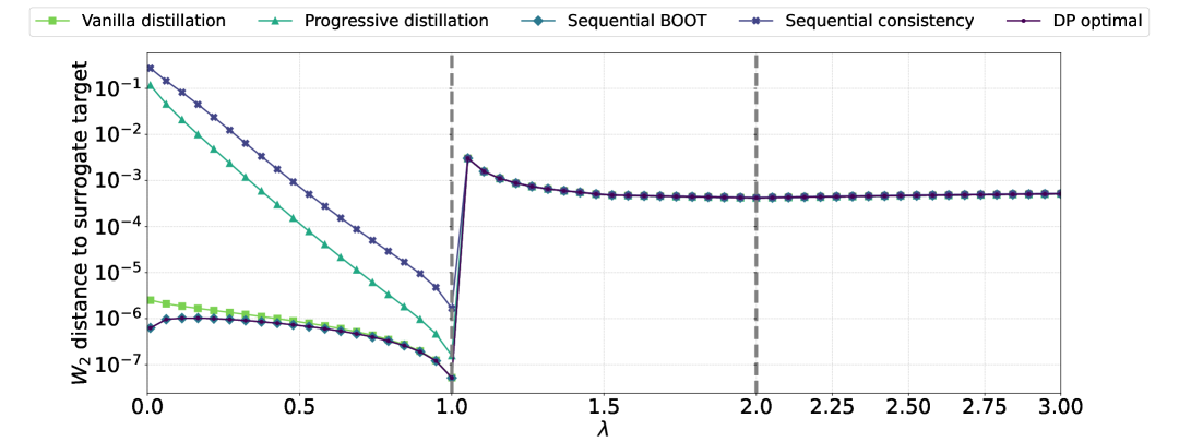
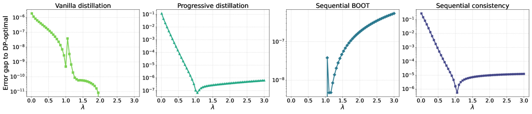
Figure 7: Evaluation of merge strategies for $T=64$ and $s=6.4$. Top: squared Wasserstein-$2$ distance between the student operator and the surrogate teacher operator under four canonical strategies (vanilla, progressive, sequential BOOT, and sequential consistency), together with the DP-optimal solution, across varying values of $\lambda$. Bottom: Error gap between each strategy and the DP-optimal baseline.

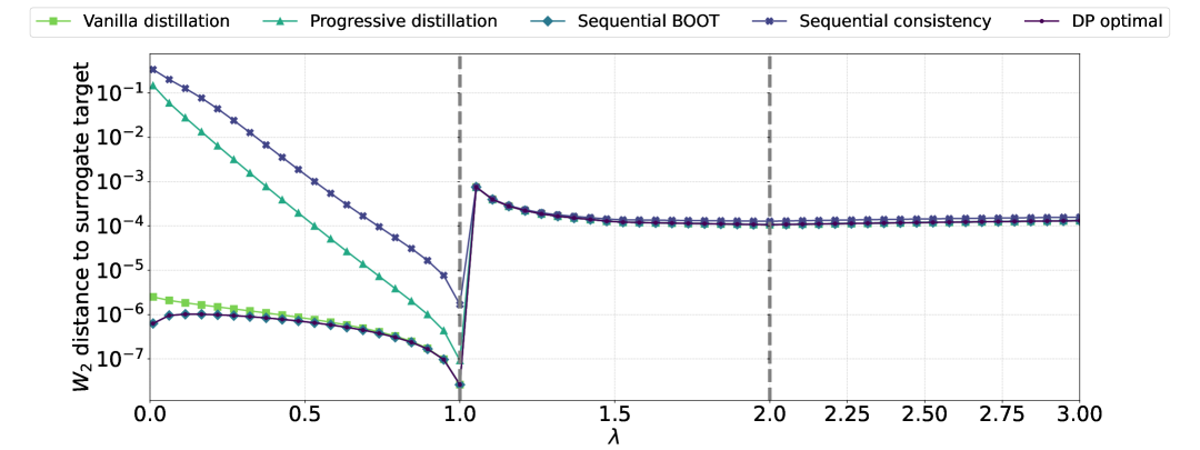
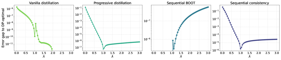
Figure 8: Evaluation of merge strategies for $T=128$ and $s=6.4$. This figure follows the same format as fig.˜7.

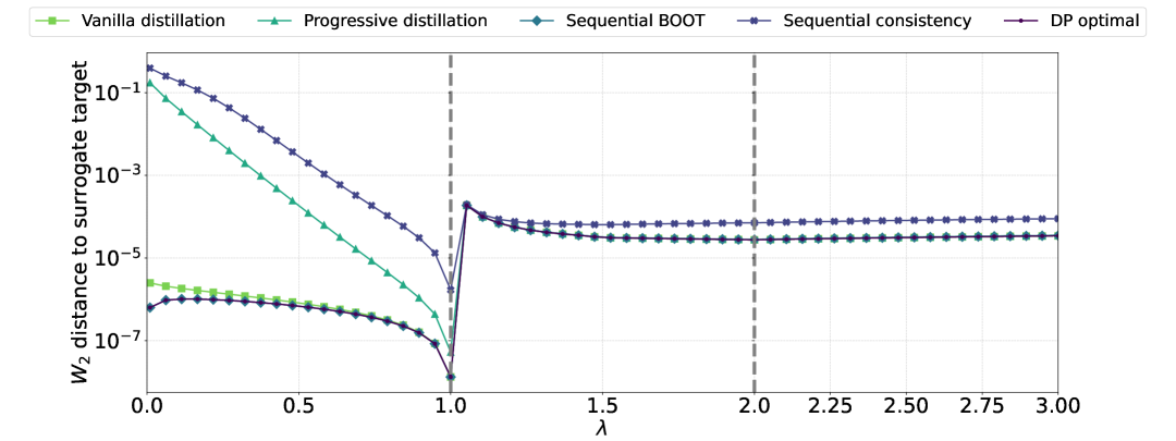
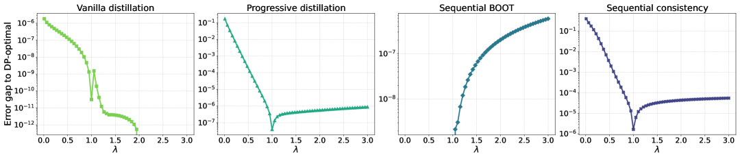
Figure 9: Evaluation of merge strategies for $T=256$ and $s=6.4$. This figure follows the same format as fig.˜7.

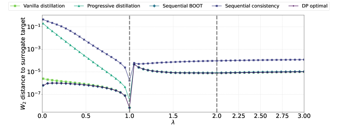
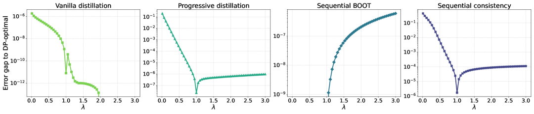
Figure 10: Evaluation of merge strategies for $T=512$ and $s=6.4$. This figure follows the same format as fig.˜7.

Dynamic programming results under different $s$.

We then present experimental results of the dynamic programming algorithm under different values of $s$, as shown in figs.˜11 and 12, complementing the special case $s=6.4$ discussed in section˜5.1. Each figure contains two panels: the top panel shows the squared Wasserstein-$2$ distance between the student operator and the surrogate teacher under four canonical strategies and the DP-optimal solution across varying $\lambda$; the bottom panel reports the corresponding error gap between each strategy and the DP baseline. Across all tested values of $s$, we observe consistent qualitative trends as in the base setting. Notably, as $s$ increases, the overall error systematically decreases across all strategies, indicating that extended training time per merge step improves the student’s ability to approximate the teacher operator.

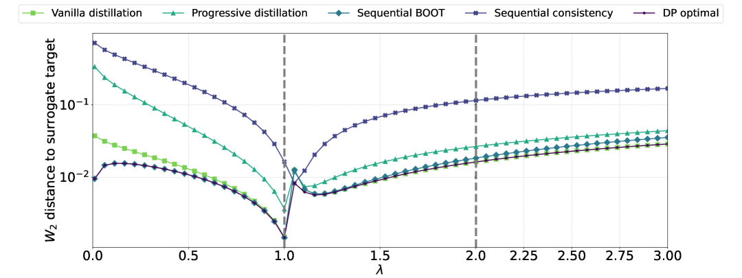
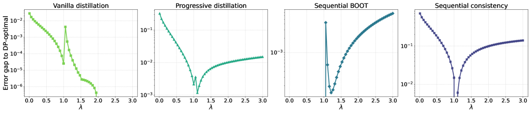
Figure 11: Evaluation of merge strategies for $T=32$ and $s=1.6$. This figure follows the same format as fig.˜7.

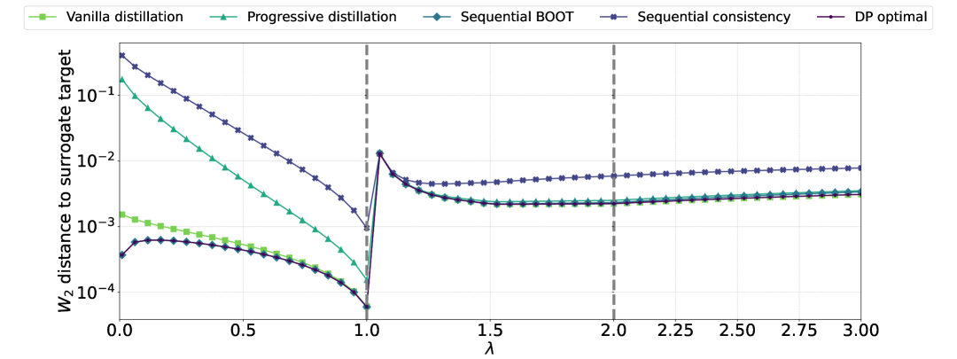
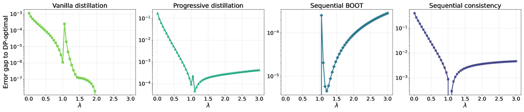
Figure 12: Evaluation of merge strategies for $T=32$ and $s=3.2$. This figure follows the same format as fig.˜7.

Dynamic programming results under different $\bm{\Lambda}$.

We further present experimental results of the dynamic programming algorithm under a range of non-scalar covariance matrices $\bm{\Lambda}=\mathrm{Diag}(\lambda_{1},\lambda_{2})$, as illustrated in fig.˜13. The specific choices of $(\lambda_{1},\lambda_{2})$ used in these experiments are summarized in table˜3. These results complement the scalar case discussed in section˜5.1. In the examples shown, we focus on “transitional” regimes, where the diagonal entries of $\bm{\Lambda}$ are neither all smaller than or equal to $1$ nor all significantly larger. These boundary regimes are already well-understood: the optimal strategy reduces to either sequential BOOT distillation or vanilla distillation, as established in the scalar setting. In contrast, as observed in fig.˜13, the transitional cases often give rise to highly intricate merging strategies that deviate from any canonical pattern.

Table 3: Transitional-regime covariance choices used in our experiments. Each pair satisfies: (i) $\lambda_{1}<\lambda_{2}$, (ii) at least one entry is near $1$, and (iii) both are not simultaneously $\leq 1$. The table is sorted by $\lambda_{1}$.

Index	1	2	3	4	5	6	7	8	9	10
$\lambda_{1}$	$0.95$	$0.95$	$0.97$	$0.98$	$0.99$	$1.00$	$1.02$	$1.02$	$1.05$	$1.08$
$\lambda_{2}$	$1.05$	$1.25$	$1.10$	$1.30$	$1.40$	$1.20$	$1.35$	$1.80$	$1.50$	$1.60$

Figure 13: Dynamic programming merge plans for a collection of transitional-regime covariance settings. Each subplot corresponds to a distinct $\bm{\Lambda}=\mathrm{Diag}(\lambda_{1},\lambda_{2})$ configuration, with the specific values labeled at the top-left corner of each plot. All choices of $(\lambda_{1},\lambda_{2})$ are summarized in table˜3, and are selected to probe transitional regimes where optimal strategies deviate from canonical forms such as vanilla or sequential BOOT. The arcs indicate the merge operations selected by the dynamic programming algorithm, where color encodes the merge order. Lighter arcs correspond to earlier merges, and darker arcs to later ones. These results demonstrate that optimal merge structures in the transitional regime are highly nontrivial and exhibit intrinsic patterns that cannot be captured by the canonical strategies.

Appendix J Additional experimental results on synthetic datasets

Computational resources.

All experiments on synthetic datasets were conducted using a single NVIDIA A30 GPU with 24 GB memory, hosted on an internal research cluster. Each student model training run took approximately 1–5 minutes, depending on the distillation strategy and covariance configuration. The full set of simulations presented in this section required approximately 20 GPU hours in total.

Table 4: Simulation results of four canonical trajectory distillation methods on synthetic datasets with varying total time steps $T$ and covariance parameter $\lambda$. Each entry reports the mean signed error (no absolute value taken) between the student operator and the surrogate composite operator $\widetilde{\mathcal{T}}_{T}$, averaged over $10$ independent trials. The best result for each setting is underlined. Results are generally consistent with our theoretical predictions in the linear regime.

$T=64$
$\lambda$	Vanilla	Progressive	BOOT	Consistency
0.20	$8.3\times 10^{-4}\pm 1.1\times 10^{-4}$	$4.5\times 10^{-2}\pm 5.6\times 10^{-4}$	$\underline{4.9\times 10^{-4}}\pm 4.8\times 10^{-5}$	$2.0\times 10^{-1}\pm 1.1\times 10^{-2}$
0.50	$4.4\times 10^{-4}\pm 9.7\times 10^{-5}$	$5.9\times 10^{-3}\pm 6.7\times 10^{-5}$	$\underline{3.2\times 10^{-4}}\pm 3.7\times 10^{-5}$	$4.8\times 10^{-2}\pm 4.5\times 10^{-3}$
1.00	$\underline{2.6\times 10^{-5}}\pm 3.0\times 10^{-6}$	$7.8\times 10^{-5}\pm 4.1\times 10^{-6}$	$2.8\times 10^{-5}\pm 4.8\times 10^{-6}$	$6.0\times 10^{-4}\pm 2.0\times 10^{-4}$
1.02	$-9.3\times 10^{-3}\pm 2.6\times 10^{-6}$	$-9.3\times 10^{-3}\pm 1.7\times 10^{-6}$	$-9.3\times 10^{-3}\pm 2.5\times 10^{-6}$	$\underline{-9.2\times 10^{-3}}\pm 1.0\times 10^{-4}$
2.00	$\underline{-8.9\times 10^{-4}}\pm 6.8\times 10^{-5}$	$-1.3\times 10^{-3}\pm 6.8\times 10^{-5}$	$-1.0\times 10^{-3}\pm 1.2\times 10^{-4}$	$-8.4\times 10^{-3}\pm 1.8\times 10^{-3}$
5.00	$\underline{-2.3\times 10^{-3}}\pm 2.0\times 10^{-4}$	$-3.0\times 10^{-3}\pm 2.8\times 10^{-4}$	$-3.0\times 10^{-3}\pm 3.7\times 10^{-4}$	$-1.3\times 10^{-2}\pm 2.5\times 10^{-3}$
$T=128$
$\lambda$	Vanilla	Progressive	BOOT	Consistency
0.20	$7.7\times 10^{-4}\pm 1.8\times 10^{-4}$	$5.6\times 10^{-2}\pm 6.0\times 10^{-4}$	$\underline{5.5\times 10^{-4}}\pm 8.0\times 10^{-5}$	$2.7\times 10^{-1}\pm 1.3\times 10^{-2}$
0.50	$3.7\times 10^{-4}\pm 5.6\times 10^{-5}$	$7.3\times 10^{-3}\pm 1.3\times 10^{-4}$	$\underline{3.3\times 10^{-4}}\pm 4.6\times 10^{-5}$	$7.4\times 10^{-2}\pm 7.7\times 10^{-3}$
1.00	$\underline{1.3\times 10^{-5}}\pm 3.1\times 10^{-6}$	$4.5\times 10^{-5}\pm 1.8\times 10^{-6}$	$1.4\times 10^{-5}\pm 2.1\times 10^{-6}$	$7.7\times 10^{-4}\pm 9.2\times 10^{-5}$
1.02	$\underline{-2.0\times 10^{-3}}\pm 8.5\times 10^{-8}$	$-2.0\times 10^{-3}\pm 4.5\times 10^{-7}$	$-2.0\times 10^{-3}\pm 6.2\times 10^{-8}$	$-2.1\times 10^{-3}\pm 3.3\times 10^{-6}$
2.00	$\underline{-6.2\times 10^{-4}}\pm 9.2\times 10^{-5}$	$-1.0\times 10^{-3}\pm 7.9\times 10^{-5}$	$-7.6\times 10^{-4}\pm 9.0\times 10^{-5}$	$-1.5\times 10^{-2}\pm 2.7\times 10^{-3}$
5.00	$\underline{-1.8\times 10^{-3}}\pm 3.5\times 10^{-4}$	$-2.8\times 10^{-3}\pm 2.3\times 10^{-4}$	$-2.3\times 10^{-3}\pm 4.3\times 10^{-4}$	$-2.3\times 10^{-2}\pm 4.4\times 10^{-3}$
$T=256$
$\lambda$	Vanilla	Progressive	BOOT	Consistency
0.20	$7.3\times 10^{-4}\pm 1.1\times 10^{-4}$	$6.7\times 10^{-2}\pm 7.6\times 10^{-4}$	$\underline{4.8\times 10^{-4}}\pm 6.8\times 10^{-5}$	$3.3\times 10^{-1}\pm 1.1\times 10^{-2}$
0.50	$4.3\times 10^{-4}\pm 7.5\times 10^{-5}$	$8.6\times 10^{-3}\pm 1.1\times 10^{-4}$	$\underline{3.2\times 10^{-4}}\pm 5.6\times 10^{-5}$	$1.2\times 10^{-1}\pm 9.2\times 10^{-3}$
1.00	$\underline{6.6\times 10^{-6}}\pm 1.2\times 10^{-6}$	$2.6\times 10^{-5}\pm 1.2\times 10^{-6}$	$7.0\times 10^{-6}\pm 1.3\times 10^{-6}$	$7.6\times 10^{-4}\pm 1.0\times 10^{-4}$
1.02	$-4.9\times 10^{-4}\pm 1.6\times 10^{-6}$	$-5.1\times 10^{-4}\pm 1.1\times 10^{-6}$	$\underline{-4.9\times 10^{-4}}\pm 9.5\times 10^{-7}$	$-1.3\times 10^{-3}\pm 1.3\times 10^{-4}$
2.00	$\underline{-5.4\times 10^{-4}}\pm 1.1\times 10^{-4}$	$-1.0\times 10^{-3}\pm 7.1\times 10^{-5}$	$-6.5\times 10^{-4}\pm 1.0\times 10^{-4}$	$-2.7\times 10^{-2}\pm 3.9\times 10^{-3}$
5.00	$\underline{-1.6\times 10^{-3}}\pm 3.4\times 10^{-4}$	$-2.8\times 10^{-3}\pm 1.6\times 10^{-4}$	$-2.7\times 10^{-3}\pm 5.2\times 10^{-4}$	$-4.3\times 10^{-2}\pm 7.6\times 10^{-3}$
$T=512$
$\lambda$	Vanilla	Progressive	BOOT	Consistency
0.20	$7.0\times 10^{-4}\pm 1.6\times 10^{-4}$	$7.9\times 10^{-2}\pm 4.9\times 10^{-4}$	$\underline{5.0\times 10^{-4}}\pm 1.0\times 10^{-4}$	$4.0\times 10^{-1}\pm 1.3\times 10^{-2}$
0.50	$4.3\times 10^{-4}\pm 8.7\times 10^{-5}$	$1.0\times 10^{-2}\pm 9.9\times 10^{-5}$	$\underline{3.4\times 10^{-4}}\pm 6.0\times 10^{-5}$	$1.7\times 10^{-1}\pm 1.4\times 10^{-2}$
1.00	$\underline{3.0\times 10^{-6}}\pm 4.4\times 10^{-7}$	$1.5\times 10^{-5}\pm 3.2\times 10^{-7}$	$3.4\times 10^{-6}\pm 6.2\times 10^{-7}$	$7.1\times 10^{-4}\pm 1.1\times 10^{-4}$
1.02	$-1.3\times 10^{-4}\pm 2.4\times 10^{-6}$	$-1.6\times 10^{-4}\pm 1.2\times 10^{-6}$	$\underline{-1.3\times 10^{-4}}\pm 1.7\times 10^{-6}$	$-2.2\times 10^{-3}\pm 2.9\times 10^{-4}$
2.00	$\underline{-5.9\times 10^{-4}}\pm 8.5\times 10^{-5}$	$-1.1\times 10^{-3}\pm 7.1\times 10^{-5}$	$-6.7\times 10^{-4}\pm 1.1\times 10^{-4}$	$-5.2\times 10^{-2}\pm 6.2\times 10^{-3}$
5.00	$\underline{-1.8\times 10^{-3}}\pm 2.8\times 10^{-4}$	$-2.9\times 10^{-3}\pm 3.7\times 10^{-4}$	$-2.4\times 10^{-3}\pm 6.4\times 10^{-4}$	$-9.2\times 10^{-2}\pm 1.3\times 10^{-2}$

Simulation results under different $T$.

We evaluate the performance of four canonical trajectory distillation strategies across a range of covariance parameters $\lambda$ and trajectory lengths $T$. All student models are implemented as sinusoidal embedding-based diagonal affine operators. For each time step $t$, the student computes a time-dependent diagonal scaling operator

$$\mathrm{Diag}\bigl{(}\bm{\theta}_{t}^{\top}\mathrm{emb}(t/T)\bigr{)},$$ (94)

where $\bm{\theta}_{t}\in\mathbb{R}^{d_{\text{emb}}\times d}$ is a learnable parameter tensor specific to time step $t$, and $\mathrm{emb}(t/T)\in\mathbb{R}^{d_{\text{emb}}}$ is the sinusoidal time embedding applied to the normalized timestep. The embedding is defined by

$$\mathrm{emb}(t/T)=\bigl{(}\sin(\omega_{1}t/T),\cos(\omega_{1}t/T),\dotsc,\sin(\omega_{d_{\text{emb}}/2}t/T),\cos(\omega_{d_{\text{emb}}/2}t/T)\bigr{)},$$ (95)

with frequencies $\omega_{i}=\frac{1}{10000^{2i/d_{\text{emb}}}}$ for $i=1,\dotsc,d_{\text{emb}}/2$. We set the embedding dimension to $d_{\text{emb}}=64$. This design enables each time step to have a distinct, smoothly varying weight. All student weights are initialized using a closed-form least-squares projection of the corresponding teacher operator. Training is performed for $100$ epochs with a batch size of $2560$, using SGD with learning rate $10^{-3}$. Each experiment is repeated independently for each $\lambda$, and the results are averaged over $10$ trials to report the mean and standard deviation. The complete set of results across different values of $T$ and $\lambda$ is summarized in table˜4.

Appendix K Additional experimental results on real dataset

Computational resources.

All experiments on the real dataset were conducted using a single NVIDIA A30 GPU with 24 GB memory. Pretraining the MSSIMVAE on the CelebA dataset took approximately 6 GPU hours. Each student model experiment (i.e., training and evaluation under one distillation strategy) required around 5 GPU hours. In total, the experiments reported in this section consumed approximately 30 GPU hours.

Experimental setup.

We first pretrain a Multiscale Structural Similarity Variational Autoencoder (MSSIMVAE) model [Snell et al., 2017] following standard settings from publicly available implementations. MSSIMVAE is a variant of the standard Variational Autoencoder (VAE) that replaces the typical pixel-wise reconstruction loss with a multiscale structural similarity (MS-SSIM) objective, encouraging perceptually meaningful reconstructions and improving latent structure.

We use the CelebA dataset [Liu et al., 2015], which contains $202{,}599$ face images, as the training data for the MSSIMVAE. After training, we extract the latent codes of the entire CelebA dataset, resulting in $202{,}599$ latent vectors, each of dimension $128$. We then compute the empirical mean and empirical covariance matrix of these latent codes.

Interestingly, we observe that the sample covariance matrix is approximately diagonal, as shown in fig.˜14, indicating that the learned latent space exhibits near-independence across dimensions. However, the diagonal entries are not uniformly equal to $1$, implying that the latent distribution is not exactly standard Gaussian $\mathcal{N}(\bm{0},\bm{I})$. Instead, the variances differ across dimensions. We extract the diagonal entries of the empirical covariance matrix and use them as target variances for our subsequent trajectory distillation experiments. Specifically, we consider the target latent distribution to be $\mathcal{N}\bigl{(}\bm{0},\mathrm{Diag}(\lambda_{1},\lambda_{2},\dotsc,\lambda_{128})\bigr{)}$, where $\lambda_{i}$ denotes the extracted variance for the $i$th latent dimension. This empirical distribution serves as a data-driven alternative to the conventional isotropic prior.

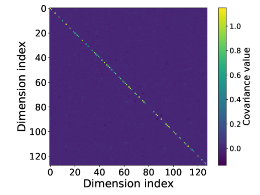
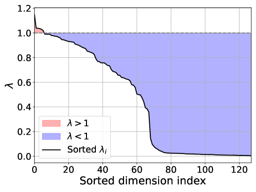
Figure 14: Covariance structure of CelebA latent codes obtained using a pretrained MSSIMVAE. Left: Heatmap of the full empirical covariance matrix. Right: Sorted diagonal entries (variances) of the covariance matrix. While the covariance matrix is approximately diagonal, the variances are not all equal to $1$, indicating that the latent distribution deviates from the standard Gaussian prior. Most diagonal entries are below $1$, and dynamic programming analysis confirms that the theoretically optimal merge strategy in this setting is sequential BOOT.

We apply different diffusion trajectory distillation strategies to generate new latent codes. Working in the latent space not only reduces the computational cost but also aligns with recent advances in generative modeling, where diffusion models are increasingly applied in learned latent spaces for efficiency and improved sample quality [Rombach et al., 2022]. Our setup mirrors this practice by distilling trajectories directly in the latent space of the pretrained MSSIMVAE.

Results.

For each trajectory distillation strategy, we compare the generated latent codes to those produced by applying the surrogate teacher composite operator under the same initial noise. All generated latent codes are decoded into images through the pretrained MSSIMVAE decoder. For reference, the decoded outputs of the surrogate teacher operator are shown in fig.˜15. These serve as the ground-truth targets for evaluating student performance. We then visualize the decoded outputs produced by the student models trained with four different strategies, i.e., vanilla, progressive, consistency, and BOOT, at three training stages: early (epoch $10$), intermediate (epochs $100$ and $1{,}000$), and converged (epoch $10{,}000$), shown in figs.˜16, 17, 18 and 19, respectively. In each figure, the left column shows the decoded outputs of the student under different strategies, while the right column presents heatmaps of the absolute difference between each student output and the corresponding teacher output. Red indicates higher deviation, while blue indicates lower deviation. The overlaid numbers report the pixel-wise $L_{2}$ distance for each case. Since all strategies operate in a shared latent space and aim to approximate the same surrogate teacher operator, it is expected that their decoded outputs appear visually similar. Nonetheless, subtle differences in operator fidelity are clearly reflected in the quantitative metrics. Across all epochs, the sequential BOOT strategy consistently achieves the lowest $L_{2}$ error, validating our theoretical prediction that it is optimal when the target covariance structure satisfies $\lambda_{i}\leq 1$ in most dimensions.

Figure 15: Reference outputs generated by the surrogate teacher operator, decoded through the pretrained MSSIMVAE. These images serve as ground-truth targets for evaluating the outputs of different distillation strategies.

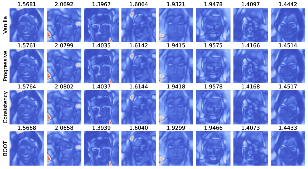
Figure 16: Comparison of decoded outputs from different distillation strategies at training epoch $10$. Left: Decoded images generated by student models trained with four different trajectory distillation strategies. From top to bottom: vanilla, progressive, consistency, and BOOT. Right: Heatmaps visualizing the absolute difference between each student output and the corresponding surrogate teacher output in pixel space. Red indicates higher deviation, while blue indicates lower deviation. The numeric label above each image denotes the corresponding pixel-wise $L_{2}$ distance.

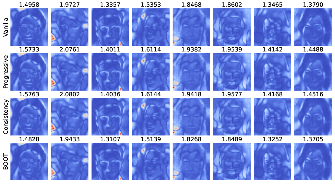
Figure 17: Comparison of decoded outputs from different distillation strategies at training epoch $100$. The visualization format is identical to fig.˜16.

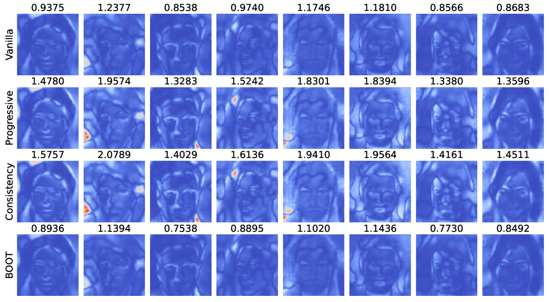
Figure 18: Comparison of decoded outputs from different distillation strategies at training epoch $1{,}000$. The visualization format is identical to fig.˜16.

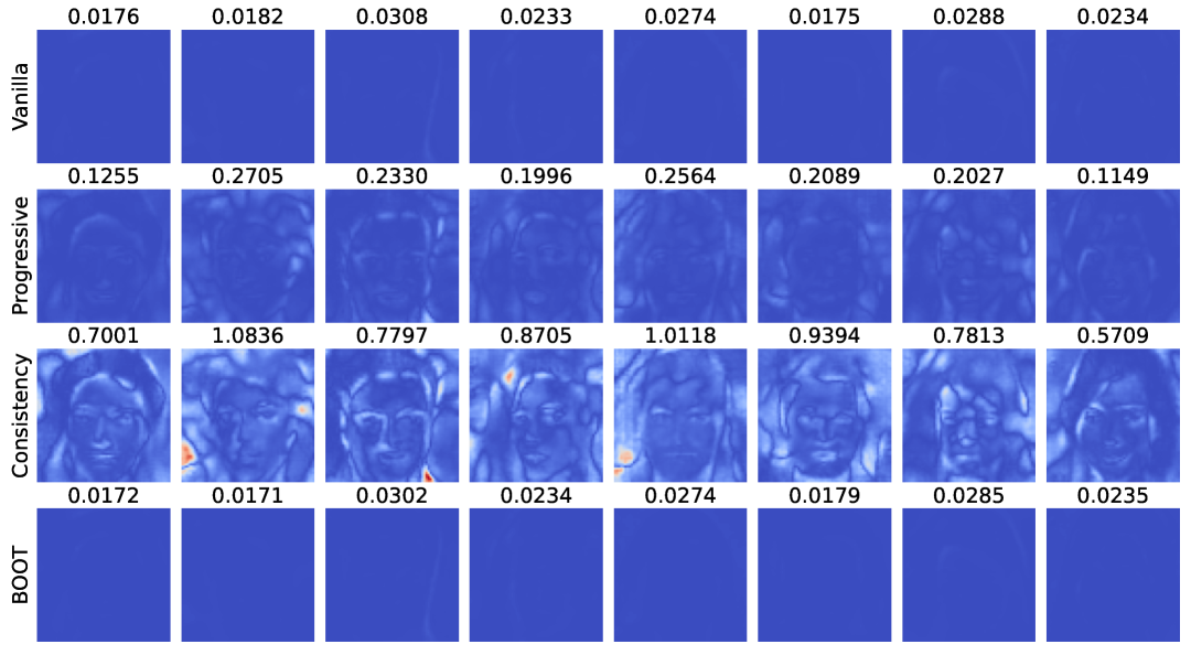
Figure 19: Comparison of decoded outputs from different distillation strategies at training epoch $10{,}000$. The visualization format is identical to fig.˜16.

Appendix L More discussions

Gaussian assumption and generalization.

Our analysis assumes that the real data distribution is a centered Gaussian with diagonal covariance, a common assumption in theoretical works [Li et al., 2024b, Wang and Vastola, 2023a, b]. Li et al. [2024b] further justify this by noting that “diffusion models in the generalization regime have inductive bias toward learning the Gaussian structures of the dataset,” suggesting that diffusion models tend to approximate Gaussian-like distributions when model capacity is not overly large.

On the practical side, while real-world unimodal datasets may not strictly follow a Gaussian distribution, they can often be effectively approximated as such. This is especially true when the data exhibits a dominant mode with small deviations, which is typical for many natural datasets. Techniques like PCA and normalization are frequently applied to make data more Gaussian-like, helping the model capture its underlying structure. Thus, the Gaussian assumption remains practical and relevant, even for non-Gaussian data.

For more complex, multimodal datasets, recent work has introduced Gaussian mixture priors [Jia et al., 2024], allowing the modeling of data with multiple modes. In this case, our analysis can be extended by treating each Gaussian component of the mixture as an individual operator. The merging process would involve combining these components while preserving their signal structure. This extension could provide a path forward for analyzing more complex data distributions.

Fixed optimization time of the student.

A key assumption in our analysis is that the student model undergoes a fixed, finite optimization time $s$ during each merge operation, resulting in signal shrinkage. This reflects real-world constraints, where the number of optimization steps is limited by time or computational budget. However, the total training time needed for a one-step student model depends on the number of merge operations. For example, one-shot distillation requires only a single merge, whereas progressive distillation involves approximately $\mathcal{O}(\log(T))$ merges.

While we focused on optimizing the student model within a fixed number of steps per merge, future research could investigate how different optimization strategies, such as curriculum learning, affect distillation quality despite limited optimization time. Additionally, exploring how various student model initialization strategies interact with optimization time could provide valuable insights into balancing efficiency and model quality.

Unaccounted aspects in the analysis.

Several practical considerations were not explicitly addressed in our analysis, though they are important for real-world applications. First, we assumed the teacher model is trained to optimality, but this may not hold when the teacher’s capacity is insufficient or when the real data distribution is complex. In these cases, it would be worth exploring whether the student model can outperform the teacher under certain conditions.

Second, the real-world training of the student model often incorporates techniques like Exponential Moving Average (EMA) to stabilize training and mixes timesteps. In contrast, our analysis assumes a sequential setting for simplicity. While EMA and similar methods are known to improve stability and generalization, their absence does not diminish the core insights on trajectory merging. Future work could integrate these techniques into our framework for more practical applications.

Lastly, the complexity of the trajectory merging process remains a topic for further exploration. As the number of steps or the size of the model increases, the computational burden of training and merging trajectories may become a limiting factor, especially for large-scale datasets or high-dimensional latent spaces. Although we focused on providing a theoretical understanding of trajectory distillation, addressing these computational challenges in future research is crucial. We believe the principles derived from our work can be adapted to handle more complex scenarios, paving the way for further advancements in trajectory distillation.

References

- Berthelot et al. (2023) D. Berthelot, A. Autef, J. Lin, D. A. Yap, S. Zhai, S. Hu, D. Zheng, W. Talbott, and E. Gu. TRACT: Denoising diffusion models with transitive closure time-distillation. arXiv preprint arXiv:2303.04248, 2023.
- Gu et al. (2023) J. Gu, S. Zhai, Y. Zhang, L. Liu, and J. M. Susskind. BOOT: Data-free distillation of denoising diffusion models with bootstrapping. In ICML 2023 Workshop on Structured Probabilistic Inference Generative Modeling, 2023.
- Ho et al. (2020) J. Ho, A. Jain, and P. Abbeel. Denoising diffusion probabilistic models. In Advances in Neural Information Processing Systems, 2020.
- Jia et al. (2024) N. Jia, T. Zhu, H. Liu, and Z. Zheng. Structured diffusion models with mixture of Gaussians as prior distribution. arXiv preprint arXiv:2410.19149, 2024.
- Karras et al. (2022) T. Karras, M. Aittala, T. Aila, and S. Laine. Elucidating the design space of diffusion-based generative models. In Advances in Neural Information Processing Systems, 2022.
- Li et al. (2024a) J. Li, W. Feng, W. Chen, and W. Y. Wang. Reward guided latent consistency distillation. Transactions on Machine Learning Research, 2024a.
- Li et al. (2024b) X. Li, Y. Dai, and Q. Qu. Understanding generalizability of diffusion models requires rethinking the hidden Gaussian structure. In Advances in Neural Information Processing Systems, 2024b.
- Lin et al. (2024) S. Lin, A. Wang, and X. Yang. SDXL-Lightning: Progressive adversarial diffusion distillation. arXiv preprint arXiv:2402.13929, 2024.
- Liu et al. (2022) L. Liu, Y. Ren, Z. Lin, and Z. Zhao. Pseudo numerical methods for diffusion models on manifolds. In International Conference on Learning Representations, 2022.
- Liu et al. (2015) Z. Liu, P. Luo, X. Wang, and X. Tang. Deep learning face attributes in the wild. In International Conference on Computer Vision, 2015.
- Lu et al. (2022a) C. Lu, Y. Zhou, F. Bao, J. Chen, C. Li, and J. Zhu. DPM-Solver: A fast ODE solver for diffusion probabilistic model sampling in around 10 steps. In Advances in Neural Information Processing Systems, 2022a.
- Lu et al. (2022b) C. Lu, Y. Zhou, F. Bao, J. Chen, C. Li, and J. Zhu. DPM-Solver++: Fast solver for guided sampling of diffusion probabilistic models. arXiv preprint arXiv:2211.01095, 2022b.
- Luhman and Luhman (2021) E. Luhman and T. Luhman. Knowledge distillation in iterative generative models for improved sampling speed. arXiv preprint arXiv:2101.02388, 2021.
- Luo et al. (2023) W. Luo, T. Hu, S. Zhang, J. Sun, Z. Li, and Z. Zhang. Diff-Instruct: A universal approach for transferring knowledge from pre-trained diffusion models. In Advances in Neural Information Processing Systems, 2023.
- Meng et al. (2023) C. Meng, R. Rombach, R. Gao, D. Kingma, S. Ermon, J. Ho, and T. Salimans. On distillation of guided diffusion models. In Proceedings of the IEEE/CVF Conference on Computer Vision and Pattern Recognition, 2023.
- Nguyen et al. (2024) B. Nguyen, B. Nguyen, and V. A. Nguyen. Bellman optimal stepsize straightening of flow-matching models. In International Conference on Learning Representations, 2024.
- Nichol and Dhariwal (2021) A. Q. Nichol and P. Dhariwal. Improved denoising diffusion probabilistic models. In International Conference on Machine Learning, 2021.
- Pei et al. (2025) J. Pei, H. Hu, and S. Gu. Optimal stepsize for diffusion sampling. arXiv preprint arXiv:2503.21774, 2025.
- Ramesh et al. (2022) A. Ramesh, P. Dhariwal, A. Nichol, C. Chu, and M. Chen. Hierarchical text-conditional image generation with CLIP latents. arXiv preprint arXiv:2204.06125, 2022.
- Ren et al. (2025) T. Ren, Z. Zhang, Z. Li, J. Jiang, S. Qin, G. Li, Y. Li, Y. Zheng, X. Li, M. Zhan, and Y. Peng. Zeroth-order informed fine-tuning for diffusion model: A recursive likelihood ratio optimizer. arXiv preprint arXiv:2502.00639, 2025.
- Rombach et al. (2022) R. Rombach, A. Blattmann, D. Lorenz, P. Esser, and B. Ommer. High-resolution image synthesis with latent diffusion models. In Proceedings of the IEEE/CVF conference on computer vision and pattern recognition, 2022.
- Saharia et al. (2022) C. Saharia, W. Chan, S. Saxena, L. Li, J. Whang, E. L. Denton, K. Ghasemipour, R. Gontijo Lopes, B. Karagol Ayan, T. Salimans, J. Ho, D. J. Fleet, and M. Norouzi. Photorealistic text-to-image diffusion models with deep language understanding. In Advances in Neural Information Processing Systems, 2022.
- Salimans and Ho (2022) T. Salimans and J. Ho. Progressive distillation for fast sampling of diffusion models. In International Conference on Learning Representations, 2022.
- Sauer et al. (2024) A. Sauer, D. Lorenz, A. Blattmann, and R. Rombach. Adversarial diffusion distillation. In European Conference on Computer Vision, 2024.
- Snell et al. (2017) J. Snell, K. Ridgeway, R. Liao, B. D. Roads, M. C. Mozer, and R. S. Zemel. Learning to generate images with perceptual similarity metrics. In International Conference on Image Processing, 2017.
- Song et al. (2021a) J. Song, C. Meng, and S. Ermon. Denoising diffusion implicit models. In International Conference on Learning Representations, 2021a.
- Song and Ermon (2019) Y. Song and S. Ermon. Generative modeling by estimating gradients of the data distribution. In Advances in Neural Information Processing Systems, 2019.
- Song et al. (2021b) Y. Song, J. Sohl-Dickstein, D. P. Kingma, A. Kumar, S. Ermon, and B. Poole. Score-based generative modeling through stochastic differential equations. In International Conference on Learning Representations, 2021b.
- Song et al. (2024) Y. Song, P. Dhariwal, M. Chen, and I. Sutskever. Consistency models. In International Conference on Learning Representations, 2024.
- Wang and Vastola (2023a) B. Wang and J. J. Vastola. Diffusion models generate images like painters: An analytical theory of outline first, details later. arXiv preprint arXiv:2303.02490, 2023a.
- Wang and Vastola (2023b) B. Wang and J. J. Vastola. The hidden linear structure in score-based models and its application. arXiv preprint arXiv:2311.10892, 2023b.
- Xu et al. (2024) C. Xu, X. Cheng, and Y. Xie. Local flow matching generative models. arXiv preprint arXiv:2410.02548, 2024.
- Xu et al. (2025) Y. Xu, W. Nie, and A. Vahdat. One-step diffusion models with -divergence distribution matching. arXiv preprint arXiv:2502.15681, 2025.
- Yin et al. (2024a) T. Yin, M. Gharbi, T. Park, R. Zhang, E. Shechtman, F. Durand, and B. Freeman. Improved distribution matching distillation for fast image synthesis. In Advances in Neural Information Processing Systems, 2024a.
- Yin et al. (2024b) T. Yin, M. Gharbi, R. Zhang, E. Shechtman, F. Durand, W. T. Freeman, and T. Park. One-step diffusion with distribution matching distillation. In Proceedings of the IEEE/CVF conference on computer vision and pattern recognition, 2024b.
- Zhao et al. (2023) W. Zhao, L. Bai, Y. Rao, J. Zhou, and J. Lu. UniPC: A unified predictor-corrector framework for fast sampling of diffusion models. In Advances in Neural Information Processing Systems, 2023.
- Zhou et al. (2024) M. Zhou, H. Zheng, Z. Wang, M. Yin, and H. Huang. Score identity distillation: Exponentially fast distillation of pretrained diffusion models for one-step generation. In International Conference on Machine Learning, 2024.
- Zhou et al. (2025) M. Zhou, H. Zheng, Y. Gu, Z. Wang, and H. Huang. Adversarial score identity distillation: Rapidly surpassing the teacher in one step. In International Conference on Learning Representations, 2025.