Holstein mechanism in single-site model with unitary evolution

Abstract

We investigate the Holstein mechanism in a single-electron (one-site) system, where unitary evolution intrinsically involves both fermion and boson operators under nonadiabatic conditions. The resulting unitary dynamics and boson-frequency dependence reveal a quantum phase transition, evidenced by distinct short-time (power-law decay) and long-time (exponential decay) behaviors, which are manifested in the polaronic shift, bosonic energy, and dynamics of reduced density matrix. This observation is consistent with a non-Markovian to Markovian transition.

I Introduction

Adiabaticity and non-adiabaticity fundamentally influence the physical properties of quantum systems, including their stability and phase transitions [1]. Unlike optical phonon modes, acoustic phonons possess lower energy (vanishing at the Brillouin zone center), providing an effective scattering channel [2]. Additionally, energy transfer to the acoustic phonon bath is the dominant cooling mechanism for a moving electron (impurity) [3]. This energy transfer relates directly to the acoustic phonon dispersion, primarily its linear component. The effect of surface optical phonons can also be explored by depositing the material on a polar substrate. In the adiabatic limit, where the electron’s Fermi velocity significantly exceeds the sound velocity, electron-phonon scattering is elastic (even in the neutral limit), and interband transitions vanish, preventing electron energy loss. However, in the nonadiabatic regime, when a non-relativistic electron moves faster than the sound wave while still interacting with acoustic phonons, it can lose energy via Cherenkov radiation. The Dirac cone inherent in 2D lattices acts as a perturbation to the free electron (impurity) in our model. The resulting mobile polaron exhibits a composite dispersion, modified by the interaction between the impurity, electron-hole pairs, and electron-phonon coupling. For weak electron-phonon coupling in the stable (adiabatic) regime, the dispersion modification is linear with the impurity momentum. Conversely, for strong electron-phonon coupling, non-adiabaticity leads to an avoided crossing in the polaron band structure. Consequently, with the absence of lattice periodicity and Brillouin zone symmetry, superfluidity may be observed at sufficiently low temperatures due where crossing Bloch bands are not hindered by the periodic lattice potential. It’s worth noting that avoided crossings also appear in ultracold Fermi atomic systems under strong-interaction limits [8, 9, 10, 11]. Phenomena dependent on impurity motion, such as coherence or decoherence, are crucial for understanding polaron formation, as they are intrinsically linked to Fermi liquid or non-Fermi liquid behavior. Decoherence can occur in extreme cases, like a very light impurity immersed in a bath of heavy particles. Conversely, for a heavy impurity in a 1D system, decoherence can also arise at zero temperature due to the orthogonality catastrophe [4, 5, 6]. In the adiabatic case, the presence of phonon absorption and emission similarly induces decoherence, reducing coherent band motion.

In this paper, we study the single-site Holstein model. Specially, a time-dependent perturbation breaks the degeneracies of original composite Hilbert spaces (electron and boson Hilbert spaces), and cause the unitary evolution of the total Hamiltonian. The perturbation not only introduces the time-dependence, but also introduces the Hermitian part to the boson operators. The Hermitian part of the boson operators not only causes the nonzero commutation between the electron term and boson term, but also causes the ground state of annihilational boson operator to deviate from the classical coherent Gaussian state. Markovian process for the system (non-adiabaticity) dominates especially in long-time limit, where the relaxation time scale of the system (exponential decay) is much slower than that of the bath electrons. While at short-time, finite non-Markovian effect with power-law decay is numerical proved, despite the fluctuations as a result of non-local correlations is absent due to the "single-site" restriction.

II Model

We consider the model described by

$$H=H_{e}+H_{b}+H_{eb},$$ (1)

where $H_{e}(t)=\epsilon U^{{\dagger}}(t)c^{{\dagger}}cU(t):=\epsilon c^{{\dagger}}(t)c(t)$ is the single electron term with $U(t)$ the unitary evolution operator. Due to the single-site consideration, the bare bandwidth is irrelevant here. Note that ${\rm Tr}[(c^{{\dagger}}(t)c(t))^{2}]={\rm Tr}[c^{{\dagger}}(t)c(t)]^{2}/N$, precluding the Hubbrd-type interacion effect. We consider the total Hamiltonian in a N-by-N Hilbert space, and a time-dependent perturbation cause breaks the degeneracies of original composite Hilbert spaces. This guarantees the unitary evolution of $H(t)$, which is distinct from the Heisenberg picture. The bosonic term reads

$$H_{b}(t)=\frac{p^{2}(t)}{2}+\frac{1}{2}\omega^{2}x^{2}(t)=\omega(b^{{\dagger}}(t)b(t)+\frac{{\bf I}}{2}),$$ (2)

where

$$b(t)=\sqrt{\frac{\omega}{2}}(x(t)+\frac{ip(t)}{\omega}),$$ (3)

$$b^{{\dagger}}(t)=\sqrt{\frac{\omega}{2}}(x(t)-\frac{ip(t)}{\omega}),$$

$$x(t)=\sqrt{\frac{1}{2\omega}}(b(t)+b^{{\dagger}}(t)),$$

$$p(t)=-i\sqrt{\frac{\omega}{2}}(b(t)-b^{{\dagger}}(t)),$$

The boson number operator $b^{{\dagger}}(t)b(t)$ is $N$-by-$N$ Hermitian matrices with a highly degenerate spectrum and are completely degenerate initially (at t=0), reflecting the internal degrees of freedom. Also, we consider the case that the fermion number operator is always at an equilibrium steady state throughout the evolution to eliminate the potential effect of its fluctuation on the polaron shift. For electron-phonon interaction, we consider the Holstein mechanism

$$H_{eb}(t)=g\omega c^{{\dagger}}(t)c(t)(b^{{\dagger}}(t)+b(t))=.g\sqrt{2\omega}\omega c^{{\dagger}}(t)c(t)x(t).$$ (4)

III Results

III.1 Polaronic shift

Different to the classical harmonic oscillator where the time-dependence of boson operator can be extracted as a phase factor, which is necessary for the Lang-Firsov transformation, the boson operator here cannot. Instead, we can separate the above boson operators (non-Hermitian) into the Hermitian part and non-Hermitian part, such that

$$b(t)=b_{H}(t)+b_{nH}(t),$$ (5)

$$b^{{\dagger}}(t)=b^{{\dagger}}_{H}(t)+b^{{\dagger}}_{nH}(t),$$

$$x(t)=x_{1}(t)+x_{2}(t)$$

$$=\sqrt{\frac{1}{2\omega}}(b_{H}(t)+b_{H}^{{\dagger}}(t))+\sqrt{\frac{1}{2\omega}}(b_{nH}(t)+b_{nH}^{{\dagger}}(t)),$$

$$p(t)=p_{1}(t)+p_{2}(t)$$

$$=-i\sqrt{\frac{\omega}{2}}(b_{H}(t)-b_{H}^{{\dagger}}(t))-i\sqrt{\frac{\omega}{2}}(b_{nH}(t)-b_{nH}^{{\dagger}}(t)),$$

where $[b_{H}(t),b^{{\dagger}}_{H}(t)]=0$ and $[b_{nH}(t),b^{{\dagger}}_{nH}(t)]=1$. Here the boson operators are still non-Hermitian and the position/momentum operators are still Hermitian. Note that ${\rm Tr}[x_{1}(t)^{2}]={\rm Tr}[x_{1}(t)]^{2}/N$ and ${\rm Tr}[x_{2}(t)^{2}]={\rm Tr}[x_{2}(t)]^{2}/N$, i.e., $x_{1}(t)$ and $x_{2}(t)$ are diagonally dominant matrices. We consider the case where the phase-space distribution remains, and as a product of the Gaussian Wigner distributions $x^{2}$ and $p^{2}$ which are inversely proportional, i.e., $\langle x^{2}\rangle=(4\langle p^{2}\rangle)^{-1}$, for the case of squeezed state at zero-temperature. This minimum uncertainty is guaranteed by the fact that both the total density matrix and the reduced one are all pure state during the evolution. Next we introduce the anti-Hermitian operator (such that $S^{{\dagger}}=-S$ and $e^{S}$ is unitary)

$$S=c^{{\dagger}}(t)c(t)(b^{{\dagger}}(t)-b(t))=\frac{\sqrt{2}}{i\sqrt{\omega}}c^{{\dagger}}(t)c(t)p(t)$$ (6)

and apply the Lang-Firsov transformation $\overline{O}=e^{S}Oe^{-S}$ to $H$, we obtain

$$\overline{H}=\epsilon c^{{\dagger}}(t)c(t)+\omega b^{{\dagger}}(t)b(t)+\frac{{\bf I}}{2}+c^{{\dagger}}(t)c(t)\Sigma(t),$$ (7)

where only the fermion number operator is invariant under the transformation. $\Sigma(t):=\Sigma_{eb}(t)+\Sigma_{b}(t)=g\omega e^{S}(b^{{\dagger}}(t)+b(t))e^{-S}+(e^{S}H_{b}e^{-S}-H_{b})H_{b}^{-1}$ is the polaronic self-energy. This definition is consistent with Ref.[7], i.e., the transformed fermion-boson term and the differece between the fermion terms after and before transformation, which measures the shift of bosonic oscillator due to the presence of electron. Note that all the expectations in this article are in the single-electron basis state $c^{{\dagger}}(t)|0\rangle$. All the numerical simulations perfomed in this article base on a 2-by-2 electron Hilbert space and 4-by-4 boson Hilbert space, such that there is 8-dimensional combined basis ($N=8$), and we adopt the convenience of notation $c^{{\dagger}}\equiv c^{{\dagger}}_{2\times 2}\otimes{\bf I}_{4\times 4}$.

Due to the intrinsic unitarility we have ${\rm Tr}H_{b}(t=0)=N\omega$ and ${\rm Tr}H_{b}(t=\infty)=\omega$, where there is a smooth exponential decay with time. For $e^{S}x(t)e^{-S}$, diagonalization through the transformation of $e^{S}$ is only successful on $x_{2}(t)$,

$$\frac{1}{g\omega N}{\rm Tr}[\Sigma_{eb}(0)]=\frac{1}{N}{\rm Tr}e^{S}(b^{{\dagger}}(t)+b(t))e^{-S}$$ (8)

$$=\frac{1}{N}{\rm Tr}e^{S}(b^{{\dagger}}_{H}(t)+b_{H}(t))e^{-S}$$

$$+\frac{1}{N}{\rm Tr}e^{S}(b_{nH}^{{\dagger}}(t)+b_{nH}(t))e^{-S}$$

$$\sim\left\{\begin{array}[]{ll}2-{\rm ln}\omega,\ (\omega<1)\\ 2+(e^{-(\omega-1)}-1)\ (\omega>1)\end{array},\right.$$

where the factor 2 originates from ${\rm Tr}[b_{H}(t=\infty)+b_{H}^{{\dagger}}(t=\infty)]=2$ (${\rm Tr}[b_{H}(t=0)+b_{H}^{{\dagger}}(t=0)]=2N$). The time and frequency dependence are important to seeking the minimal of polaronic shift. For $\omega\leq 1$ and at finite time,

$$\frac{1}{g\omega N}{\rm Tr}[\Sigma_{eb}(t)]=\frac{1}{N}{\rm Tr}e^{S}(b^{{\dagger}}(t)+b(t))e^{-S}$$ (9)

$$=\frac{1}{N}{\rm Tr}e^{S}(b^{{\dagger}}_{H}(t)+b_{H}(t))e^{-S}$$

$$+\frac{1}{N}{\rm Tr}e^{S}(b_{nH}^{{\dagger}}(t)+b_{nH}(t))e^{-S}$$

$$\sim\left\{\begin{array}[]{ll}(2-{\rm ln}\omega)\frac{\omega}{t},\ (small\ t)\\ (2-{\rm ln}\omega)e^{-t/\omega}\ (large\ t)\end{array}\right.+\left\{\begin{array}[]{ll}(2-{\rm ln}\omega)\frac{\omega}{t^{1/\omega}},\ (small\ t)\\ -\frac{(2-{\rm ln}\omega)e^{-t/\omega}+1}{\omega}\ (large\ t)\end{array},\right.$$

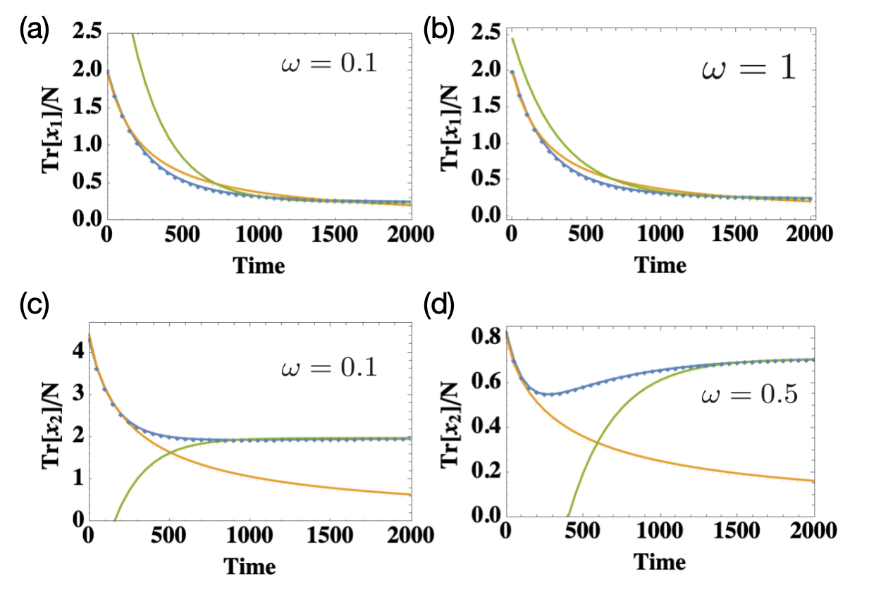
Figure 2: Expectations of $x_{1}(t)$ and $x_{2}(t)$.

where the early stage and latter stage follow the power-law decay and exponential decay, respectively. This is shown in Fig.2, in terms of the boson dispalcement. While for the boson number operator (which is frequency-independent),

$${\rm Tr}[b^{{\dagger}}(t)b(t)] \sim\left\{\begin{array}[]{ll}\frac{1}{t+\frac{1}{N}},\ (small\ t)\\ 1+e^{-t}\ (large\ t),\end{array}\right.$$ (10)

as shown in Fig.1(a). As a result, the expectation of $H_{b}$ on the single electron basis state is linear on $\omega$. Thus the observables’ trace exhibit the transition from power-law decay to exponential decay with time evolution, signifying the corresponding system density’s dynamics (Lindbladian) be gappless in the begining, and be gapped at long-time. Note that during the whole process the spectrum of Lindbladian should be purely real (without the component of oscillation frequencies) due to the absence of non-local correlations and coherence (hopping of electron) for $\omega\leq 1$.

III.2 Effect of transformation to the boson operators

Since both the fermion operator and boson operator share the same unitary dynamics, they are not mutually commute unless remove the Hermitian part of the boson operators. The difference of position operator before and after transformation, $\sqrt{2\omega}\Delta x(t):=e^{S}(b^{{\dagger}}(t)+b(t))e^{-S}-(b^{{\dagger}}(t)+b(t))$ which is a diagonalizable defective matrix, is not soly determined by the fermion operator due to the contribution from $[b^{{\dagger}}_{nH}(t)-b_{nH}(t),b^{{\dagger}}_{H}(t)+b_{H}(t)]$. The lowered rank signifies the existence of states insensitive to the perturbations (reminiscent of the dark states). Further, since $e^{S}(b^{{\dagger}}(t)+b(t))^{2}e^{-S}=((b^{{\dagger}}(t)+b(t))+\sqrt{2\omega}\Delta x(t))^{2}$, we have

$${\rm Tr}[2\omega\Delta x(t)^{2}]+2{\rm Tr}[(b^{{\dagger}}(t)+b(t))\sqrt{2\omega}\Delta x(t)]=0,$$ (11)

where for $\omega\leq 1$, we obtain

$${\rm Tr}[2\omega\Delta x(t)^{2}]\sim\left\{\begin{array}[]{ll}0,\ (small\ t)\\ \omega(1-e^{-t})\ (large\ t)\end{array}\right.$$ (12)

which is linear in $\omega$ at long time. The exact result of ${\rm Tr}[2\omega\Delta x(t)^{2}]$ is shown in Fig.3. We also obtain its approximated result in appendix. Fluctuations signifying non-local correlations can be seen in Fig.4, we can apply another transformation using $S^{\prime}=c^{{\dagger}}(0)c(t)(b^{{\dagger}}(t)-b(t))$, which is nomore a anti-Hermitian operator as long as $t\neq 0$.

IV Dynamics of reduced density matrix

We next focus on the dynamics of reduced density matrix $\rho_{e}={\rm Tr}_{b}\rho_{tot}$ (partial trace over the bosonic bases) where $\rho_{tot}=|\psi_{0}\rangle\langle\psi_{0}|$ with $|\psi_{0}\rangle$ the eigenstate of $H$ corresponding to lowest eigenvalue, i.e., $\rho_{tot}=\sum_{ij}c_{i}c_{j}^{*}|\Psi_{i}\rangle\langle\Psi_{j}|$ where $c_{i}$ is the $i$-th component of $|\psi_{0}\rangle$, and $|\Psi_{i}\rangle$ is the $i$-th state of the combined basis. Note that the rank of $H$ is lowered with increasing time, in this case we use $\rho_{tot}=\frac{1}{d}\sum_{j=1}^{d}|\psi_{0}\rangle\langle\psi_{0}|$ with $d$ the ground state degeneracy, in which case it requires further orthonormalized to keeping ${\rm Tr}\rho_{e}=1$. While for $\rho_{tot}$ in mixed state which corresponds to the case of finite temperature, we have $\rho_{tot}=\sum_{j}e^{-\beta E_{j}}|\psi_{j}\rangle\langle\psi_{j}|/\sum_{j}e^{-\beta E_{j}}$. But we stick to the zero temperature case in this paper, thus we do not adopt this mixed state. The resulting reduced electron density $\rho_{e}$ is a 2-by-2 Hermitian matrix, with the two diagonal elements describe the populations of two states in electron Hilbert space, and the two off-diagonal elements describe the coherence between the two states. The result shows that, at short-time (far before the emergence of degenerated ground state of $H$), $\rho_{e;11}\sim{\rm ln}t(=1-\rho_{e;22})$, and reasonably, $\frac{d\rho_{e;11}}{dt}\sim\frac{1}{t}(=-\frac{d\rho_{e;22}}{dt})$, as shown in Fig.5. The logarithmic increase in population $\rho_{e;11}$ reflects a extremely slow dynamics, and the system is not reaching a steady state. The power-law decay in $\frac{d\rho_{e;11}}{dt}$ again signifying the Non-Markovian Memory effect in early stage during the evolution. While exponential decay emerges at longer time (but before the emergence of degenerated ground state of $H$), $\rho_{e;11}\sim-e^{-t}$ and $\frac{d\rho_{e;11}}{dt}\sim e^{-t}$.

From Fig.5, one also notice that the $\rho_{e;11}$ is quite large and increase with time, instead of decrease, which means $\rho_{e}$ and $\rho_{b}$ are close to purity state and the purity increase with time. This main seems in contrast to the conclusion we obtained elsewhere, i.e., the Markovian process as well as the decoherence dominates at the long-time and implying the enhanced entanglement. This is because we initially choose the boson number operator with degenerated spectrum, which means the states do not distinguished by the particle number (population) but the internal degrees of freedom. When the perturbation weakly breaks the degeneracy, purity of the corresponding density matrix increases. Thus, the purity of the reduced density matrices does not affect our above conclusions. Meanwhile, their dynamics support our conclusions (where the internal degrees of freedom plays the main role). Also, by virtue of the high purity of the reduced density matrices, we gain the convenience of not needing to consider the deviation from the minimum uncertainty condition in the phase space.

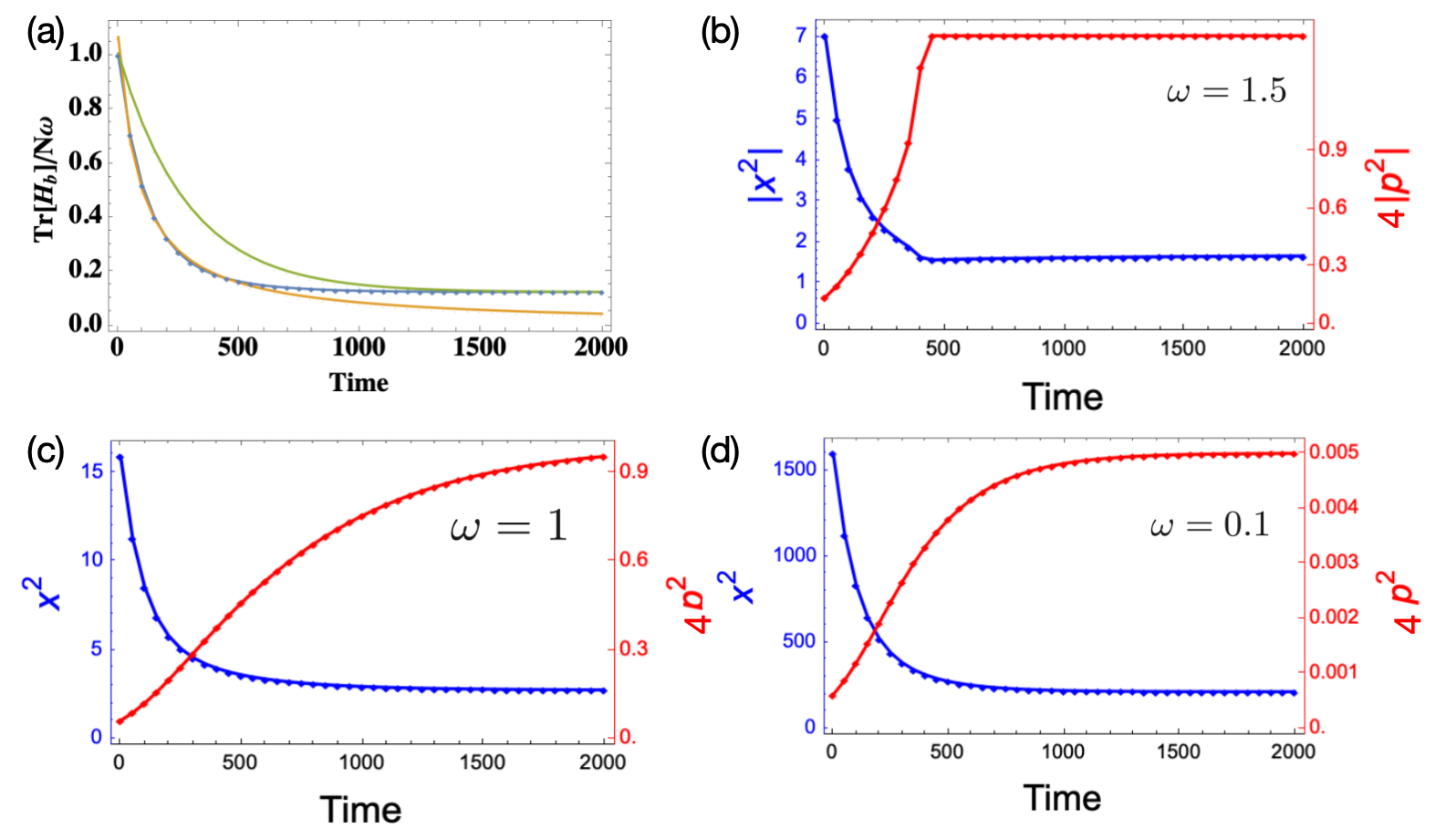
Figure 1: (a) Expectation of boson operator on the single electron basis state, which relaxes toward $\frac{1}{N}$ at long-time. (b)-(d) Expectations of position and momentum operators which follow the Gaussian Wigner distributions. (b) shows the case $\omega>1$ where the imaginary part of squared position and momentum operators emerges (this is also the regime where there is nonzero real part of expectation of momentum operator).

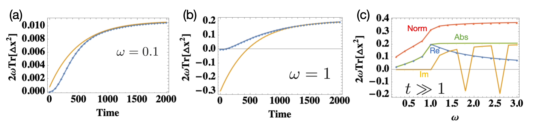
Figure 3: Expectations of $\Delta x^{2}$ as a function of time ((a)-(b)) and frequency ((c)). Above the critical frequency $\omega_{c}=1$, the real part star to decline and nonzero imaginary part emerges.

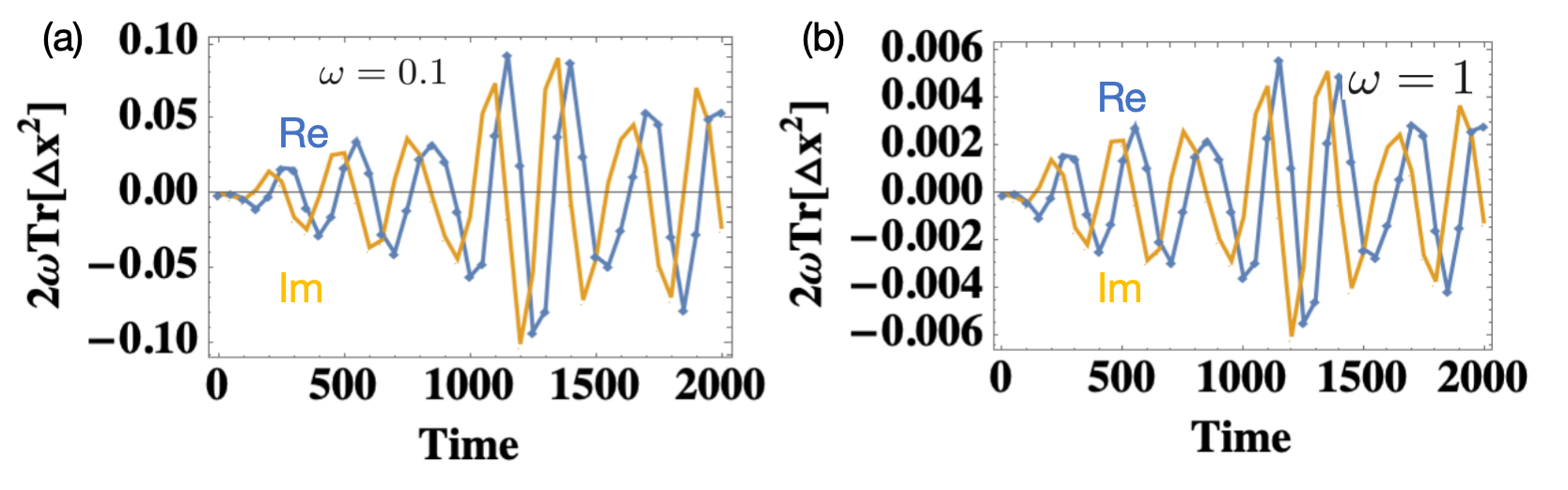
Figure 4: The same with Fig.3 (a)-(b) but replacing the $S$ by $S^{\prime}$.

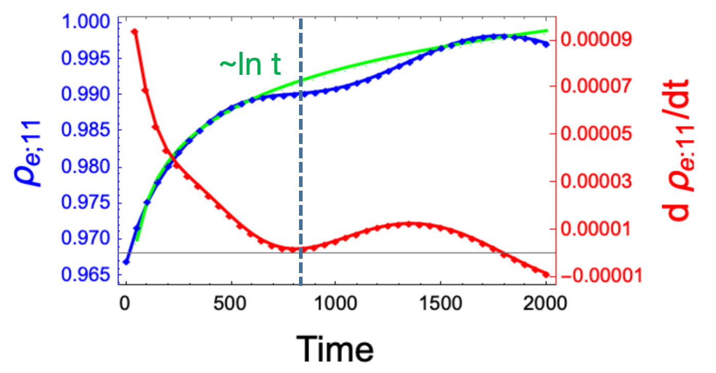
Figure 5: First diagonal element of the reduced density matrix $\rho_{e}$ and its time derivative. The vertical dashed line indicate the time where the degenerated ground states of $H$ emege.

V Conclusion

We consider the electron-phonon coupling in single electron (one-site) system with unitary evolution that is intrinsic to the boson operators in the case of nonadiabatic limit. We consider the case where the phase-space distribution remains, and as a product of the Gaussian Wigner distributions $x^{2}$ and $p^{2}$ which are inversely proportional, i.e., $\langle x^{2}\rangle=(4\langle p^{2}\rangle)^{-1}$, for the case of squeezed state at zero-temperature. This minimum uncertainty is guaranteed by the fact that both the total density matrix and the reduced one are nearly pure state during the evolution (i.e., ${\rm Tr}[\rho_{e}^{2}]={\rm Tr}[\rho_{tot}^{2}]\approx 1$, which means there is weak entanglement in this bipartite system despite such entanglement slightly enhanced at long-time due to the rised Markovian and decoherence process). The unitary dynamics preserves the phase-space distribution during the Markovian process wth slow relaxation, and the electron-phonon interaction dominates over the influences from bath electrons. In this limit, the Gaussian wave function fail to describe bosons which can no longer be treated as classical field, and phononic time scale is much faster than the electronic time scale. The mean-field theory also fails to be applied in this case. The unitary dynamics as well as boson-frequency-dependence provides the evidence of quantum phase transition from the distinct behaviors at short-time and long-time stages, which exhibit power law and exponential law decay, respectively, as can be seen from the polaronic shift, boson energy, and the dynamics of reduced density $\rho_{e}$. Moreover, the effective mass renormalization $m^{*}/m(=e^{\Sigma(t)/\omega})$ should follow the same rule, despite not being shown here. The gradual opening of the dissipative gap can be further verified by estimating the Lindbladian’s spectrum. This estimation, achievable through Lanczos iteration or the quantum trajectory method, as well as the case of boson squeezing ($(b^{{\dagger}})^{2}+b^{2}$) and the deviation away from minimum uncertainty condition (entanglement increase the classical uncertainty), will be the scope of our next work.

VI Appendix: Approximation form of ${\rm Tr}[2\omega\Delta x(t)^{2}]$

Using the following relations

$${\rm Tr}[(e^{S}(b^{{\dagger}}(t)+b(t))e^{-S})^{2}]={\rm Tr}[(b^{{\dagger}}(t)+b(t))^{2}]={\rm Tr}[e^{S}(b^{{\dagger}}(t)+b(t))^{2}e^{-S}],$$ (13)

$${\rm Tr}[e^{S}(b^{{\dagger}}(t)+b(t))e^{-S}(b^{{\dagger}}(t)+b(t))]={\rm Tr}[(b^{{\dagger}}(t)+b(t))e^{S}(b^{{\dagger}}(t)+b(t))e^{-S}],$$

$${\rm Tr}[e^{S}(b^{{\dagger}}(t)+b(t))e^{S}(b^{{\dagger}}(t)+b(t))e^{-S}]={\rm Tr}[(b^{{\dagger}}(t)+b(t))^{2}e^{S}]={\rm Tr}[(b^{{\dagger}}(t)+b(t))^{2}e^{-S}]^{*}$$

$$={\rm Tr}[e^{S}(b^{{\dagger}}(t)+b(t))^{2}]={\rm Tr}[e^{-S}(b^{{\dagger}}(t)+b(t))^{2}]^{*}$$

we can obtain

$${\rm Tr}[e^{S}(b^{{\dagger}}(t)+b(t))^{2}e^{-S}]-{\rm Tr}[e^{S}(b^{{\dagger}}(t)+b(t))e^{-S}(b^{{\dagger}}(t)+b(t))]={\rm Tr}[e^{S}(b^{{\dagger}}(t)+b(t))[(b^{{\dagger}}(t)+b(t)),e^{-S}]]$$ (14)

$$={\rm Tr}[e^{S}(b^{{\dagger}}(t)+b(t))(-[(b^{{\dagger}}(t)+b(t)),S]+\sum_{n=2}\frac{(-1)^{n}}{n!}[(b^{{\dagger}}(t)+b(t)),S^{n}])]$$

$$={\rm Tr}[e^{S}(b^{{\dagger}}(t)+b(t))(e^{S}(b^{{\dagger}}(t)+b(t))e^{-S}-(b^{{\dagger}}(t)+b(t))-\sum_{n=2}\frac{1}{n!}[S^{(n)},(b^{{\dagger}}(t)+b(t))]+\sum_{n=2}\frac{(-1)^{n}}{n!}[(b^{{\dagger}}(t)+b(t)),S^{n}])]$$

$$={\rm Tr}[e^{S}(b^{{\dagger}}(t)+b(t))(-\sum_{n=2}\frac{1}{n!}[S^{(n)},(b^{{\dagger}}(t)+b(t))]+\sum_{n=2}\frac{(-1)^{n}}{n!}[(b^{{\dagger}}(t)+b(t)),S^{n}])]=\frac{1}{2}{\rm Tr}[2\omega\Delta x(t)^{2}].$$

where $S^{(n)}$ denote $n$-th order commutator. Then we have

$${\rm Tr}[2\omega\Delta x(t)^{2}]=-2{\rm Tr}[e^{S}(b^{{\dagger}}(t)+b(t))S[S,(b^{{\dagger}}(t)+b(t))]]+O(S^{3}).$$ (15)

References

- [1] Altman E, Auerbach A. Oscillating superfluidity of bosons in optical lattices[J]. Physical review letters, 2002, 89(25): 250404.
- [2] Hwang E H, Sarma S D. Acoustic phonon scattering limited carrier mobility in two-dimensional extrinsic graphene[J]. Physical Review B, 2008, 77(11): 115449.
- [3] Bistritzer R, MacDonald A H. Electronic cooling in graphene[J]. Physical Review Letters, 2009, 102(20): 206410.
- [4] Rosch A, Kopp T. Heavy particle in a d-dimensional fermionic bath: A strong coupling approach[J]. Physical review letters, 1995, 75(10): 1988.
- [5] Kantian A, Schollw?ck U, Giamarchi T. Competing regimes of motion of 1D mobile impurities[J]. Physical review letters, 2014, 113(7): 070601.
- [6] Meden V, Schmitteckert P, Shannon N. Orthogonality catastrophe in a one-dimensional system of correlated electrons[J]. Physical Review B, 1998, 57(15): 8878.
- [7] Hohenadler, Martin, and Wolfgang von der Linden. "Lang-Firsov approaches to polaron physics: From variational methods to unbiased quantum Monte Carlo simulations." Polarons in Advanced Materials. Dordrecht: Springer Netherlands, 2007. 463-502.
- [8] Fetherolf, Jonathan H., Denis Golež, and Timothy C. Berkelbach. "A unification of the Holstein polaron and dynamic disorder pictures of charge transport in organic crystals." Physical Review X 10.2 (2020): 021062.
- [9] Alexandrov, A. S. "Polaron dynamics and bipolaron condensation in cuprates." Physical Review B 61.18 (2000): 12315.
- [10] Ooi, CH Raymond, and KJ Cedric Chia. "Unified master equation for molecules in phonon and radiation baths." Scientific reports 12.1 (2022): 20015.
- [11] Pausch, Lukas, et al. "How to seed ergodic dynamics of interacting bosons under conditions of many-body quantum chaos." Reports on Progress in Physics (2025).