A broken-FEEC framework for structure-preserving discretizations of polar domains with tensor-product splines

Abstract

We propose a novel projection-based approach to derive structure-preserving Finite Element Exterior Calculus (FEEC) discretizations using standard tensor-product splines on domains with a polar singularity. This approach follows the main lines of broken-FEEC schemes which define stable and structure-preserving operators in non-conforming discretizations of the de Rham sequence. Here, we devise a polar broken-FEEC framework that enables the use of standard tensor-product spline spaces while ensuring stability and smoothness for the solutions, as well as the preservation of the de Rham structure: A benefit of this approach is the ability to reuse codes that implement standard splines on smooth parametric domains, and efficient solvers such as Kronecker-product spline interpolation. Our construction is based on two pillars: the first one is an explicit characterization of smooth polar spline spaces within the tensor-product splines ones, which are either discontinuous or non square-integrable as a result of the singular polar pushforward operators. The second pillar consists of local, explicit and matrix-free conforming projection operators that map general tensor-product splines onto smooth polar splines, and that commute with the differential operators of the de Rham sequence.

1 Introduction

In computational electromagnetism, finite element discretizations that preserve the de Rham structure play a fundamental role in developing stable and accurate numerical schemes [1, 2, 3]. These discretizations also ensure the conservation of essential physical properties such as the Hamiltonian structure of Vlasov-Maxwell equations [4, 5], while naturally accommodating curvilinear geometries through the use of parametric mappings and pushforward operators [2, 6]. One particularly effective class of methods employs tensor-product splines, which can be assembled into stable sequences of discrete differential forms [7].

When dealing with polar parametrizations, which are especially convenient for disk- or torus-shaped domains, a well-known issue arises: because of the singularity exhibited by the mapping determinant at the pole, the pushforward tensor-product splines have poor smoothness or integrability properties, thereby preventing their use in practical computations.

This challenge has been previously addressed in the literature, notably by Toshniwal and co-authors who proposed a construction of smooth polar splines in [8]. By defining proper extraction matrices which correspond to the coefficients of the smooth splines in the full (a priori singular) tensor-product basis, this construction results in splines which are smooth on a surface parametrized by a spline polar mapping, and in [9] it has been extended to smooth rational splines on spheres and ellipsoids. The construction of polar splines for the different spaces of a de Rham sequence was then proposed in [10] for polar spline surfaces, and in [11] for toroidal spline domains. In [12], commuting projection operators have been proposed for axisymmetric toroidal domains with a polar spline cross section. Overall, these works provide reduced spline spaces that allow for stable, structure-preserving approximations of de Rham sequences on domains with polar singularities.

In this article, we propose an alternative approach which allows to design structure-preserving schemes with standard tensor-product spline spaces. Our method relies on discrete projection operators which map the tensor-product splines spaces onto the smooth polar ones. In particular, it allows to reuse standard finite element matrices associated with usual tensor-product B-splines, without the need to re-implement new operators in a reduced basis.

A key property of our conforming projections is to commute with the de Rham sequence: this ensures that the resulting discretization maintains the desired structural properties, and it further allows to apply commuting projections based on interpolation and histopolation by inverting Kronecker products of univariate collocation matrices.

Such a projection-based approach was first introduced in the CONGA (conforming/non-conforming Galerkin) scheme for Maxwell’s equations [13]. There, it was applied to represent the electric fields in discontinuous function spaces in order to allow for local (block-diagonal) mass matrices and inverse Hodge operators. Later it was extended to the discontinuous discretization of the full de Rham sequence in [14]. In the resulting broken-FEEC framework, generic Hodge operators (such as weighted $L^{2}$ projections) are local, as well as the dual differential operators and the dual commuting projections.

Here, we follow the same ideas to handle the singularities induced by the pushforward operators associated with a spline polar mapping. A main ingrendient of our approach is an explicit characterization of the smooth spline spaces in terms of their tensor-product spline coefficients. This characterization then allows for a simple description of local projection operators onto the conforming spaces, which are then shown to possess the desired commuting properties.

The remainder of the article is organized as follows. In Section 2 we recall the main steps of the projection-based broken-FEEC method for structure-preserving discretizations with non-conforming finite element spaces, and we further specify in which sense tensor-product splines are not conforming after a pushforward on a domain with a polar singularity. In Section 3 we then present our main results, which are threefold: (i) a characterization of the conforming spline de Rham subcomplexes corresponding to $H^{1}$ and $C^{1}$ potential spaces respectively, (ii) sequences of explicit conforming projection operators mapping tensor-product splines onto the $H^{1}$ and $C^{1}$ subcomplexes, and (iii) new sequences of commuting projection operators onto these subcomplexes, obtained by composing our discrete conforming projections with geometric interpolations in the tensor-product spline spaces. The characterization of the smooth spline subcomplexes is proven in Section 4, and after studying the integrability and commuting properties of the pullback and pushforward operators in Section 5, we prove the commuting properties of our conforming projections in Section 6, as well as those of the tensor-product geometric projections on the polar domain. Finally we illustrate our construction with several numerical experiments in Section 7. Our results confirm that isogeometric polar broken-FEEC approximations of Poisson and Maxwell’s equations using the proposed projection matrices yield stable and high-order accurate solutions.

2 Principles of broken-FEEC schemes on domains with a polar singularity

2.1 Conforming discretizations of de Rham sequences in $\mathbb{R}^{2}$

Structure-preserving finite element discretizations of two-dimensional domains usually involve discrete de Rham sequences of the form

(1)

where the finite-dimensional spaces $V^{\ell}_{h}$ are conforming, i.e., subspaces of the natural spaces $V^{\ell}$ involved in the underlying continuous problem. A common choice is to define the latter as the Hilbert de Rham sequence [3]:

(2)

We note that in $\mathbb{R}^{2}$ there exists another de Rham sequence, namely

(3)

which can be related to the grad-curl sequence by a standard rotation argument: indeed, we have

$$\operatorname{{\bf curl}}\phi=R\operatorname{{\bf grad}}\phi\quad\text{ and }\quad\operatorname{{div}}{\boldsymbol{v}}=\operatorname{{curl}}R^{-1}{\boldsymbol{v}}\quad\text{ with}\quad R=\begin{pmatrix}0&1\\ -1&0\end{pmatrix}.$$ (4)

In this article we will consider discretizations of the grad-curl sequence (2), but we note that that all our results readily apply to to the div-curl sequence (3) through a rotation of the vector fields.

2.2 Projection approach for non-conforming FEEC spaces

In practice, it may be convenient to work with non-conforming spaces

$$W^{\ell}_{h}\not\subset V^{\ell}\quad\text{ such that }\quad V^{\ell}_{h}=W^{\ell}_{h}\cap V^{\ell}$$

such as fully discontinuous spaces (which have block-diagonal mass matrices). The broken-FEEC approach then relies on discrete conforming projections

$$P^{\ell}:W^{\ell}_{h}\to V^{\ell}_{h}$$ (5)

which yield a new, non-conforming de Rham sequence

(6)

This framework allows to derive stable numerical approximations in so-called broken-FEEC spaces for many problems in electromagnetism, as described for instance in [14]. A simple example is the Poisson equation,

$$\left\{\begin{array}[]{rl}-\Delta\phi=f&\quad\text{in }\Omega\\ \phi=0&\quad\text{on }\partial\Omega.\end{array}\right.$$ (7)

By adding homogeneous boundary conditions to the definition of the spaces (2), and hence to the conforming projections (5), one can approximate the solution to (7) by a non-conforming potential $\phi_{h}\in W^{0}_{h}$ satisfying

$$\langle\operatorname{{\bf grad}}P^{0}\phi_{h},\operatorname{{\bf grad}}P^{0}\psi_{h}\rangle+\alpha\langle(I-P^{0})\phi_{h},(I-P^{0})\psi_{h}\rangle=\langle f,P^{0}\psi_{h}\rangle$$ (8)

for all $\psi_{h}\in W^{0}_{h}$. Similarly, the electric field solving Maxwell’s time harmonic equation

$$\left\{\begin{array}[]{rl}(-\omega^{2}+\operatorname{{curl}}\operatorname{{curl}}){\boldsymbol{E}}={\boldsymbol{J}}&\quad\text{in }{\Omega}\\ {\boldsymbol{n}}\times{\boldsymbol{E}}=0&\quad\text{on }\partial\Omega,\end{array}\right.$$ (9)

can be approximated by a non-conforming discrete field ${\boldsymbol{E}}_{h}\in W^{1}_{h}$ solution to

$$-\omega^{2}\langle P^{1}{\boldsymbol{E}}_{h},P^{1}{\boldsymbol{F}}_{h}\rangle+\langle\operatorname{{curl}}P^{1}{\boldsymbol{E}}_{h},\operatorname{{curl}}P^{1}{\boldsymbol{F}}_{h}\rangle+\alpha\langle(I-P^{1}){\boldsymbol{E}}_{h},(I-P^{1}){\boldsymbol{F}}_{h}\rangle=\langle{\boldsymbol{J}},P^{1}{\boldsymbol{F}}_{h}\rangle$$ (10)

for all ${\boldsymbol{F}}_{h}\in W^{1}_{h}$. For both problems above, one shows that for any stabilization parameter $\alpha>0$ the non-conforming solutions actually belong to the conforming spaces and solve the conforming Galerkin problems [14].

Non-conforming approximations to time-dependent problems can also be derived, for instance Maxwell’s equations

$$\left\{\begin{array}[]{rl}\partial_{t}{\boldsymbol{E}}-\operatorname{{curl}}{\boldsymbol{B}}&=-{\boldsymbol{J}}\\ \partial_{t}{\boldsymbol{B}}+\operatorname{{curl}}{\boldsymbol{E}}&=0\end{array}\right.$$ (11)

which can be discretized in space as

$$\left\{\begin{array}[]{rl}\langle\partial_{t}{\boldsymbol{E}}_{h},{\boldsymbol{F}}_{h}\rangle-\langle{\boldsymbol{B}}_{h},\operatorname{{curl}}P^{1}{\boldsymbol{F}}_{h}\rangle&=-\langle{\boldsymbol{J}},P^{1}{\boldsymbol{F}}_{h}\rangle\\ \partial_{t}{\boldsymbol{B}}_{h}+\operatorname{{curl}}P^{1}{\boldsymbol{E}}_{h}&=0\end{array}\right.$$ (12)

for all test function ${\boldsymbol{F}}_{h}\in W^{1}_{h}$. As this discretization has no stabilization mechanism its solution does not belong to the conforming space, however it is stable and shown to preserve a discrete version of the Gauss law $\operatorname{{div}}{\boldsymbol{E}}=\rho$, see [13].

Remark 2.1.

Here we have implicitely assumed that the non-conforming functions where square integrable, i.e., that $W^{\ell}_{h}\subset L^{2}(\Omega)$. Although this inclusion holds for non-conforming spaces that result from a relaxation of the continuity constraints across regular interfaces as studied in [14], it is no longer be the case for the non-conforming spaces considered in this article, which result from a singular mapping. This issue will be addressed in Section 3.7 below.

2.3 Domains with a polar singularity

In this article we consider problems posed on a polar domain, that is an open domain $\Omega\subset\mathbb{R}^{2}$ whose closure $\overline{\Omega}$ is the image of the logical annulus $\hat{\Omega}\coloneqq[0,L]\times(\mathbb{R}/2\pi\mathbb{Z})$ by a $C^{1}$ surjective mapping

$$F:\hat{\Omega}\ni\begin{pmatrix}s\\ \theta\end{pmatrix}\mapsto{\boldsymbol{x}}\in\overline{\Omega}$$ (13)

that collapses the logical edge $\{0\}\times(\mathbb{R}/2\pi\mathbb{Z})$ (simply denoted $\{s=0\}$ hereafter) to a single point ${\boldsymbol{x}}_{0}\in\Omega$, which we will call the pole. We further assume that $F$ induces a $C^{1}$ diffeomorphism between the punctured polar domain and its preimage, namely

$$\overline{\Omega}_{0}\coloneqq\overline{\Omega}\setminus\{{\boldsymbol{x}}_{0}\}\qquad\text{ and }\qquad\hat{\Omega}_{0}\coloneqq\hat{\Omega}\setminus\{s=0\}=F^{-1}(\overline{\Omega}_{0}).$$ (14)

Here we will consider two types of such polar mappings:

• the “analytical” polar mapping

  $$F:\begin{pmatrix}s\\ \theta\end{pmatrix}\mapsto{\boldsymbol{x}}_{0}+\begin{pmatrix}s\cos\theta\\ s\sin\theta\end{pmatrix}$$ (15)

  corresponding to a disk domain $\Omega=\Omega_{\rm disk}$,

• a spline mapping of the form

  $$F:\begin{pmatrix}s\\ \theta\end{pmatrix}\mapsto{\boldsymbol{x}}_{0}+\sum_{i=0}^{n_{s}-1}\sum_{j=0}^{n_{\theta}-1}\boldsymbol{P}_{ij}B_{i}(s)\mathring{B}_{j}(\theta)$$ (16)

  with regular B splines along the periodic variable $\theta$ as described below, and regular control points close to the pole, i.e.

  $$\boldsymbol{P}_{ij}=\begin{pmatrix}\rho_{i}\cos\theta_{j}\\ \rho_{i}\sin\theta_{j}\end{pmatrix}~~\text{ for }~~\left\{\begin{aligned} &i\in\{0,1\}\\ &0\leq j<n_{\theta}\end{aligned}\right.~~\text{ with }~~\left\{\begin{aligned} &0=\rho_{0}<\rho_{1}\\ &\theta_{j}\coloneqq j\Delta_{\theta},~\Delta_{\theta}\coloneqq\tfrac{2\pi}{n_{\theta}}~.\end{aligned}\right.$$ (17)

In (16), $B_{i}$ and $\mathring{B}_{j}$ are B-splines of degree $p\geq 1$ in the respective $s$ and $\theta$ variables (the upper ring denoting a periodic spline). B-splines along $s$ are defined by an open knot sequence

$$s_{0}=\cdots=s_{p}<s_{p+1}<\cdots<s_{n_{s}-1}<s_{n_{s}}=\cdots=s_{n_{s}+p}=L,$$ (18)

and along $\theta$ we use the regular angles $\theta_{j}=j\Delta_{\theta}$ as knots (extended to all $j\in\mathbb{Z}$ by periodicity). We note that the above assumption of $F$ being a $C^{1}$ diffeomorphism between the domains (14) implies

$$\det J_{F}(s,\theta)>0\qquad\text{ for all $s>0$ and all $\theta$}.$$ (19)

In addition, we make the following assumption on the spline resolution along $\theta$.

Assumption 2.2.

In the case of a spline mapping (16)–(17), the number of (regular) knots $\theta_{j}$ satisfies

$$n_{\theta}=4n^{\prime}\qquad\text{ with an integer }n^{\prime}\geq p\geq 1.$$ (20)

This assumption will be useful for studying the strength of the mapping singularity in Proposition 2.5 below. It will also allow us to use standard discrete trigonometry relations that are reminded in the Appendix, together with some details on B-splines.

Remark 2.3.

Using standard tools [7], our results directly extend to any smooth deformations of the above domains, that is, to any mapping of the form $G\circ F$ where $G$ is a smooth diffeomorphism and $F$ is one of the polar mappings above.

The singularity of polar mappings can be characterized as follows.

Definition 2.4.

We say that a mapping $F$ has a first order polar singularity if the following properties hold:

• its Jacobian matrix is of the form

  $$J_{F}(s,\theta)=\begin{pmatrix}C(\theta)+\mathcal{O}(s)&s(C^{\prime}(\theta)+\mathcal{O}(s))\\ S(\theta)+\mathcal{O}(s)&s(S^{\prime}(\theta)+\mathcal{O}(s))\end{pmatrix},\quad\det J_{F}(s,\theta)=s(D(\theta)+\mathcal{O}(s))$$ (21)

  where $C$ and $S$ are $C^{1}$ functions, $D(\theta)=(CS^{\prime}-SC^{\prime})(\theta)>0$ holds for all $\theta$. Here we use the classical notation $\mathcal{O}(s)$ to denote a generic function (depending a priori on $s$ and $\theta$, and which value may change at each occurence) satisfying

  $$\lvert\mathcal{O}(s)\rvert\leq cs$$ (22)

  for some constant $c>0$ that may depend on the mapping parameters.

• the bound $sD_{*}\leq\det J_{F}(s,\theta)$ holds for a positive constant $D_{*}>0$, and the inverse Jacobian determinant is of the form

  $$\det J_{F}^{-1}(s,\theta)=\frac{1+\mathcal{O}(s)}{sD(\theta)},$$ (23)

  again for a generic function $\mathcal{O}(s)$ satisfying (22).

Proposition 2.5.

Both the analytical mapping (15) and the generic spline mapping (16) (assuming (19)) have a first order polar singularity in the sense of Definition 2.4.

Proof.

The Jacobian matrix reads

$$J_{F}(s,\theta)=\begin{pmatrix}\partial_{s}F_{1}(s,\theta)&\partial_{\theta}F_{1}(s,\theta)\\ \partial_{s}F_{2}(s,\theta)&\partial_{\theta}F_{2}(s,\theta)\end{pmatrix}.$$ (24)

In the case of the analytical mapping (15) we thus have

$$J_{F}(s,\theta)=\begin{pmatrix}\cos\theta&-s\sin\theta\\ \sin\theta&s\cos\theta\end{pmatrix},\qquad\det J_{F}(s,\theta)=s,$$ (25)

which yields (21) with $C(\theta)=\cos\theta$, $S(\theta)=\sin\theta$, $D(\theta)=1$ and $\mathcal{O}(s)=0$.

In the case of the spline mapping (16), we apply the derivative formula (123) from the Appendix to write

$$\left\{\begin{aligned} \partial_{s}F_{1}(s,\theta)&=\sum_{i=0}^{n_{s}-2}(\rho_{i+1}-\rho_{i})M_{i}(s)\sum_{j=0}^{n_{\theta}-1}\cos\theta_{j}\mathring{B}_{j}(\theta)\\ \partial_{\theta}F_{1}(s,\theta)&=\sum_{i=0}^{n_{s}-1}\rho_{i}B_{i}(s)\Big{(}\sum_{j=0}^{n_{\theta}-1}\cos\theta_{j}\mathring{B}_{j}\Big{)}^{\prime}(\theta)\\ \partial_{s}F_{2}(s,\theta)&=\sum_{i=0}^{n_{s}-2}(\rho_{i+1}-\rho_{i})M_{i}(s)\sum_{j=0}^{n_{\theta}-1}\sin\theta_{j}\mathring{B}_{j}(\theta)\\ \partial_{\theta}F_{2}(s,\theta)&=\sum_{i=0}^{n_{s}-1}\rho_{i}B_{i}(s)\Big{(}\sum_{j=0}^{n_{\theta}-1}\sin\theta_{j}\mathring{B}_{j}\Big{)}^{\prime}(\theta).\end{aligned}\right.$$ (26)

Using the relations (125)–(126) (also from the Appendix) satisfied at the pole, and the fact that $\rho_{0}=0$, we further see that

$$\sum_{i=0}^{n_{s}-2}(\rho_{i+1}-\rho_{i})M_{i}(s)=\rho_{1}M_{0}(0)+\mathcal{O}(s)\quad\text{ and }\quad\sum_{i=0}^{n_{s}-1}\rho_{i}B_{i}(s)=s(\rho_{1}M_{0}(0)+\mathcal{O}(s))$$

hold with a function $\mathcal{O}(s)$ satisfying (22). This yields (21) with

$$C(\theta)=\rho_{1}M_{0}(0)\sum_{j=0}^{n_{\theta}-1}\cos\theta_{j}\mathring{B}_{j}(\theta)\quad\text{ and }\quad S(\theta)=\rho_{1}M_{0}(0)\sum_{j=0}^{n_{\theta}-1}\sin\theta_{j}\mathring{B}_{j}(\theta).$$ (27)

To show that $D(\theta)=(CS^{\prime}-SC^{\prime})(\theta)$ is positive for all $\theta$, we compute

$$\begin{split}\frac{D(\theta)}{(\rho_{1}M_{0}(0))^{2}}&=\sum_{j,k=0}^{n_{\theta}-1}\Big{(}\cos\theta_{j}(\sin\theta_{k+1}-\sin\theta_{k})\mathring{B}_{j}\mathring{M}_{k}-(\cos\theta_{j+1}-\cos\theta_{j})\sin\theta_{k}\mathring{M}_{j}\mathring{B}_{k}\Big{)}(\theta)\\ &=\sum_{j,k=0}^{n_{\theta}-1}\big{(}(\cos\theta_{j}\sin\theta_{k+1}-\sin\theta_{j}\cos\theta_{k+1})-(\cos\theta_{j}\sin\theta_{k}-\cos\theta_{k}\sin\theta_{j})\big{)}\mathring{B}_{j}\mathring{M}_{k}(\theta)\\ &=\sum_{j,k=0}^{n_{\theta}-1}(\sin\theta_{k-j+1}-\sin\theta_{k-j})\mathring{B}_{j}\mathring{M}_{k}(\theta)\\ &=\sum_{j=0}^{n_{\theta}-1}\sum_{k=-p}^{p-1}(\sin\theta_{k+1}-\sin\theta_{k})\mathring{B}_{j}\mathring{M}_{j+k}(\theta)\end{split}$$

where in the last equality we have used (130) to reduce the second sum. By the mean value theorem, for all $k\in\{-p,\ldots,p-1\}$ there exists $\bar{\theta}_{k}\in(\theta_{k},\theta_{k+1})\subset(-\theta_{p},\theta_{p})$ such that $\sin\theta_{k+1}-\sin\theta_{k}=\Delta\theta\cos\bar{\theta}_{k}$ and from the inequality $n_{\theta}\geq 4p$ derived from (20), we infer that $\theta_{p}=\frac{2\pi p}{n_{\theta}}\leq\frac{\pi}{2}$. In particular, we have $\lvert\bar{\theta}_{k}\rvert<\frac{\pi}{2}$ for all $k$, hence

$$\sin\theta_{k+1}-\sin\theta_{k}=\Delta\theta\cos\bar{\theta}_{k}>0\quad\text{ for }\quad k\in\{-p,\ldots,p-1\}.$$

The bound $D(\theta)>0$ follows from the non-negativity of the B and M basis splines. Observe that if $n_{\theta}>4p$, we have $\sin\theta_{k+1}-\sin\theta_{k}=\Delta\theta\cos\bar{\theta}_{k}>\Delta\theta\cos\theta_{p},$ hence, using (124) and (129),

$$\frac{D(\theta)}{(\rho_{1}M_{0}(0))^{2}}\geq\sum_{j,k}\Delta\theta\cos\theta_{p}\mathring{B}_{j}(\theta)\mathring{M}_{j+k}(\theta)\geq\cos\theta_{p}>0$$

which gives a uniform bound with respect to $n_{\theta}$ (note that $\cos\theta_{p}\to 1$ as $n_{\theta}\to\infty$). The bounds on $\det J_{F}$, as well as the form (23), follow easily by using this lower bound on $D(\theta)$ and the assumption (19). ∎

2.4 Singularity of the tensor-product spline de Rham sequence

On the logical domain we consider a de Rham sequence of tensor-product splines [7], of the form

$$\hat{W}^{0}_{h}:=\SS_{p,p}(\hat{\Omega})\xrightarrow{\mbox{$~\operatorname{\widehat{\bf grad}}~$}}\hat{W}^{1}_{h}:=\begin{pmatrix}\SS_{p-1,p}(\hat{\Omega})\\ \SS_{p,p-1}(\hat{\Omega})\end{pmatrix}\xrightarrow{\mbox{$~\operatorname{\widehat{curl}}~$}}\hat{W}^{2}_{h}:=\SS_{p-1,p-1}(\hat{\Omega}).$$ (28)

Here the hatted derivatives correspond to the logical variables $(s,\theta)\in\hat{\Omega}$, and $\SS_{p_{1},p_{2}}(\hat{\Omega}):=\SS_{p_{1}}([0,L])\otimes\SS_{p_{2}}(\mathbb{R}/2\pi\mathbb{Z})$ are tensor-product spline spaces associated with the same breakpoints as the spline mapping (16). These spaces are classically equipped with tensor-product spline bases,

$$\left\{\begin{aligned} \text{ for }\hat{W}^{0}_{h}:\quad&{\hat{T}}^{0}_{ij}(s,\theta)=B_{i}(s)\mathring{B}_{j}(\theta)\\ \text{ for }\hat{W}^{1}_{h}:\quad&{\hat{\boldsymbol{T}}}_{ij}^{s}(s,\theta)=\begin{pmatrix}M_{i}(s)\mathring{B}_{j}(\theta)\\ 0\end{pmatrix}~\text{ and }~{\hat{\boldsymbol{T}}}_{ij}^{\theta}(s,\theta)=\begin{pmatrix}0\\ B_{i}(s)\mathring{M}_{j}(\theta)\end{pmatrix}\\ \text{ for }\hat{W}^{2}_{h}:\quad&{\hat{T}}^{2}_{ij}(s,\theta)=M_{i}(s)\mathring{M}_{j}(\theta).\end{aligned}\right.$$ (29)

involving the B and M splines defined in the Appendix. On the “physical” polar domain $\Omega$, the standard approach [2, 7, 15] consists in pushing forward the logical spaces (28), i.e., setting

$$W^{0}_{h}\coloneqq\mathcal{F}^{0}\hat{W}^{0}_{h},\qquad W^{1}_{h}\coloneqq\mathcal{F}^{1}\hat{W}^{1}_{h},\qquad W^{2}_{h}\coloneqq\mathcal{F}^{2}\hat{W}^{2}_{h}$$ (30)

with pushforward operators defined as

$$\left\{\begin{aligned} &\mathcal{F}^{0}:\hat{\phi}\mapsto\phi:=\hat{\phi}\circ F^{-1}\\ &\mathcal{F}^{1}:\hat{\boldsymbol{v}}\mapsto{\boldsymbol{v}}:=\big{(}J_{F}^{-T}\hat{\boldsymbol{v}}\big{)}\circ F^{-1}\\ &\mathcal{F}^{2}:\hat{f}\mapsto f:=\big{(}\det J_{F}^{-1}\hat{f}\big{)}\circ F^{-1}.\end{aligned}\right.$$ (31)

This amounts to defining the physical spaces as the span of the pushforward tensor-product spline basis functions:

$$\left\{\begin{aligned} W^{0}_{h}&=\operatorname{Span}\Big{(}\big{\{}T^{0}_{ij}\coloneqq\mathcal{F}^{0}{\hat{T}}^{0}_{ij}:0\leq i<n_{s},0\leq j<n_{\theta}\big{\}}\Big{)}\\ W^{1}_{h}&=\operatorname{Span}\Big{(}\big{\{}{\boldsymbol{T}}_{ij}^{s}\coloneqq\mathcal{F}^{1}{\hat{\boldsymbol{T}}}_{ij}^{s}:0\leq i<n_{s}-1,0\leq j<n_{\theta}\big{\}}\\ &\mspace{100.0mu}\cup\big{\{}{\boldsymbol{T}}_{ij}^{\theta}\coloneqq\mathcal{F}^{1}{\hat{\boldsymbol{T}}}_{ij}^{\theta}:0\leq i<n_{s},0\leq j<n_{\theta}\big{\}}\Big{)}\\ W^{2}_{h}&=\operatorname{Span}\Big{(}\big{\{}T^{2}_{ij}\coloneqq\mathcal{F}^{2}{\hat{T}}^{2}_{ij}:0\leq i<n_{s}-1,0\leq j<n_{\theta}\big{\}}\Big{)}.\end{aligned}\right.$$ (32)

Since $F:\hat{\Omega}_{0}\to\overline{\Omega}_{0}$ is a $C^{1}$ diffeomorphism, (31) defines bijective operators between continuous functions away from the pole, that is,

$$\mathcal{F}^{\ell}:C^{0}(\hat{\Omega}_{0})\to C^{0}(\overline{\Omega}_{0})\quad\text{ is a bijection for $\ell\in\{0,1,2\}$}$$

with inverse operators $\mathcal{B}^{\ell}:C^{0}(\overline{\Omega}_{0})\to C^{0}(\hat{\Omega}_{0})$ called pullbacks,

$$\left\{\begin{aligned} &\mathcal{B}^{0}:\phi\mapsto\hat{\phi}:=\phi\circ F\\ &\mathcal{B}^{1}:{\boldsymbol{v}}\mapsto\hat{\boldsymbol{v}}:=J_{F}^{T}({\boldsymbol{v}}\circ F)\\ &\mathcal{B}^{2}:f\mapsto\hat{f}:=\det J_{F}(f\circ F).\end{aligned}\right.$$ (33)

On the full polar domain, i.e. when the pole is included, one easily verifies that the pullbacks are actually well-defined.

Proposition 2.6.

The pullbacks $\mathcal{B}^{\ell}$ are continuous mappings from $L^{q}(\Omega)$ to $L^{q}(\hat{\Omega})$, $1\leq q\leq\infty$, as well as from $C^{0}(\overline{\Omega})$ to $C^{0}(\hat{\Omega})$.

Proof.

Simply use the bounds (21) on the mapping Jacobian $J_{F}$. ∎

A key property of regular pullbacks and pushforward is the commutation with the differential operators from de Rham sequence (2), see e.g. [2]. Away from the pole, this commutation also holds here for general smooth functions: for any $\hat{\phi}$ and $\hat{\boldsymbol{v}}$ in $C^{1}(\hat{\Omega})$, the equalities

$$\operatorname{{\bf grad}}\mathcal{F}^{0}\hat{\phi}=\mathcal{F}^{1}\operatorname{\widehat{\bf grad}}\hat{\phi}\quad\text{ and }\quad\operatorname{{curl}}\mathcal{F}^{1}\hat{\boldsymbol{v}}=\mathcal{F}^{2}\operatorname{\widehat{curl}}\hat{\boldsymbol{v}}\quad\text{ hold on }\Omega_{0},$$ (34)

where we remind that $\Omega_{0}$ is the punctured domain (14), and that the hatted derivatives correspond to the logical variables $(s,\theta)\in\hat{\Omega}$. We point out that here, the logical functions $\hat{\phi}$ and $\hat{\boldsymbol{v}}$ are assumed to be smooth up to $s=0$, however (34) does not a priori hold on the full polar domain $\Omega$ because of the singularity of the pushforward operators: First, one may have that $\mathcal{F}^{0}\hat{\phi}\notin H^{1}(\Omega)$ or even that $\mathcal{F}^{1}\hat{\boldsymbol{v}}\notin L^{2}(\Omega)$ for smooth functions on $\hat{\Omega}$. Second, the relations (34) (and in particular the second one) do not hold for all smooth functions on $\hat{\Omega}$. The latter issue will be analyzed in Proposition 5.5. The former one can be stated as follows.

Proposition 2.7.

The spaces (30) are not a conforming discretization of (2), in the sense that

$$W^{0}_{h}\not\subset H^{1}(\Omega),\qquad W^{1}_{h}\not\subset L^{2}(\Omega),\qquad W^{2}_{h}\not\subset L^{2}(\Omega).$$

Proof.

The functions in $W^{0}_{h}$ are bounded on the bounded domain $\Omega$ so they are $L^{2}(\Omega)$, however their gradient may not be. To verify this, consider a spline that does not vanish on the pole, such as $\phi=\mathcal{F}^{0}{\hat{T}}_{0j}^{0}$ with an arbitrary $j$, that is $\phi({\boldsymbol{x}})=B_{0}(s)\mathring{B}_{j}(\theta)$ with ${\boldsymbol{x}}=F(s,\theta)$, and use the commutation relation (34) for ${\boldsymbol{x}}\in\Omega_{0}$, i.e. $s>0$: with the derivative formulas (123) and (128) from the Appendix, this gives

$$\operatorname{{\bf grad}}\phi({\boldsymbol{x}})=(\mathcal{F}^{1}\operatorname{\widehat{\bf grad}}{\hat{T}}_{0j}^{0})({\boldsymbol{x}})=J_{F}^{-T}(s,\theta)\begin{pmatrix}-M_{0}(s)\mathring{B}_{j}(\theta)\\ B_{0}(s)(\mathring{M}_{j-1}(\theta)-\mathring{M}_{j}(\theta))\end{pmatrix}$$

with a matrix of the form

$$J_{F}^{-T}(s,\theta) =\frac{1}{\det J_{F}}\begin{pmatrix}\partial_{2}F_{2}&-\partial_{1}F_{2}\\ -\partial_{2}F_{1}&\partial_{1}F_{1}\end{pmatrix}(s,\theta)$$

$$=\frac{1}{s(D(\theta)+\mathcal{O}(s))}\begin{pmatrix}s(S^{\prime}(\theta)+\mathcal{O}(s))&-S(\theta)+\mathcal{O}(s)\\ -s(C^{\prime}(\theta)+\mathcal{O}(s))&C(\theta)+\mathcal{O}(s)\end{pmatrix}$$

where the second equality uses (21). Using Equation (23) and $B_{0}(s)=1+\mathcal{O}(s)$, this implies that

$$\operatorname{{\bf grad}}\phi({\boldsymbol{x}})=\frac{{\boldsymbol{G}}(\theta)}{s}+\boldsymbol{g}({\boldsymbol{x}})\quad\text{ with }\quad{\boldsymbol{G}}(\theta)\coloneqq\frac{1}{D(\theta)}\begin{pmatrix}-S(\theta)(\mathring{M}_{j-1}(\theta)-\mathring{M}_{j}(\theta))\\ C(\theta)(\mathring{M}_{j-1}(\theta)-\mathring{M}_{j}(\theta))\end{pmatrix}$$

and some bounded $\boldsymbol{g}\in L^{\infty}(\Omega)$. This easily shows that $\operatorname{{\bf grad}}\phi\notin L^{2}(\Omega)$, indeed

$$\int_{\Omega}\lvert\operatorname{{\bf grad}}\phi({\boldsymbol{x}})-\boldsymbol{g}({\boldsymbol{x}})\rvert^{2}\,\mathrm{d}{\boldsymbol{x}}=\int_{\hat{\Omega}}\frac{\lvert{\boldsymbol{G}}(\theta)\rvert^{2}}{s^{2}}\det J_{F}(s,\theta)\,\mathrm{d}s\,\mathrm{d}\theta\\ =\int_{\hat{\Omega}}\frac{\lvert{\boldsymbol{G}}(\theta)\rvert^{2}}{s}(D(\theta)+\mathcal{O}(s))\,\mathrm{d}s\,\mathrm{d}\theta=+\infty.$$ (35)

The same argument (replacing $\operatorname{{\bf grad}}\phi$ by $\mathcal{F}^{1}\boldsymbol{T}_{0j}^{\theta}$) shows that $W^{1}_{h}\not\subset L^{2}(\Omega)$. Finally the non-inclusion for the space $W^{2}_{h}$ is verified by considering $f=\mathcal{F}^{2}{\hat{T}}_{0j}^{2}$, which, using again Equation (23), writes as

$$f({\boldsymbol{x}})=\det J^{-1}_{F}{\hat{T}}_{0j}^{2}(s,\theta)=\frac{M_{0}(s)\mathring{M}_{j}(\theta)}{\det J_{F}}=\frac{G(\theta)}{s}+g({\boldsymbol{x}})$$

with $G(\theta)=\frac{M_{0}(0)\mathring{M}_{j}(\theta)}{D(\theta)}$ and a bounded $g\in L^{\infty}(\Omega)$. One clearly has $f\notin L^{2}(\Omega)$. ∎

3 Construction of a polar broken-FEEC framework with tensor-product splines

3.1 Work plan

As a consequence of Proposition 2.7, we see that the tensor-product spaces $W^{\ell}_{h}$ are not suitable for finite element methods. They are suitable, however, for applying the projection-based broken-FEEC approach described in Section 2. To do so we need to specify conforming spline spaces, and propose discrete projection operators that map arbitrary tensor-product splines onto the conforming subspaces. In addition, we will require that our conforming projections are local (only coefficients close to the pole should be modified) and commuting: this will be detailed just below.

In this article we will consider two notions of conformity: the first one corresponds to the simplest (maximal) Hilbert sequence (2), that is

(36)

and the second one consists of smoother functions, namely

(37)

In the sequel we will refer to (36) and (37) as the $H^{1}$ and $C^{1}$ sequences, respectively. To each of these sequences, that is for $Z=V$ or $U$, we associate conforming subspaces

$$Z^{\ell}_{h}\coloneqq W^{\ell}_{h}\cap Z^{\ell},\quad\text{ $\ell=0,1,2$.}$$ (38)

Our first task will be provide an explicit characterization of these subspaces in terms of their tensor-product spline coefficients, and our second task will be to design local conforming projections of the form

$$P^{\ell}_{Z}:W^{\ell}_{h}\to Z^{\ell}_{h},$$ (39)

that is, operators which satisfy $P^{\ell}_{Z}W^{\ell}_{h}=Z^{\ell}_{h}$ and $(P^{\ell}_{Z})^{2}=P^{\ell}_{Z}$ and which only modify spline coefficients close to the pole.

A third task will be to build projection operators $\Pi^{\ell}_{Z}$ onto the discrete spaces $Z^{\ell}_{h}$, for which the following diagram commutes:

(40)

Commuting projections play indeed an important role in the preservation of certain structure properties at the discrete level: they allow to write discrete Hodge-Helmholtz decompositions with proper harmonic field spaces of the correct dimension [3], or to preserve the Hamiltonian structure in variational particle discretization of Vlasov-Maxwell equations [5]. Note that in (40) the operators $\Pi^{\ell}_{Z}$ may be unbounded, in the sense that their domains $D(\Pi^{\ell}_{Z})$ may be proper subspaces of the spaces from the top row, typically consisting of smoother functions. Nevertheless, these domains need to be dense: we therefore need to extend the projections $P^{\ell}_{Z}$ to infinite-dimensional spaces.

We observe that commuting projection operators on polar spline spaces have already been proposed in [12], by introducing special sets of geometric degrees of freedom close to the pole. In this work we will propose an alternative construction which takes advantage of (and preserves) the tensor-product structure of the underlying spline spaces.

A classical way to obtain commuting projections is indeed to interpolate geometric degrees of freedom, as is done by the De Rham map and described in [16, 17]: the commuting properties of the resulting projection then essentially follows from the Stokes theorem. On the Cartesian domain $\hat{\Omega}$, this approach yields logical geometric projections $\hat{\Pi}^{\ell}_{W}$ on the tensor-product spline spaces, which are fast to evaluate thanks to the Kronecker structure of the collocation matrices to be inverted. We will review their main properties in Section 3.3. Their counterparts on the physical domain, namely

$$\Pi^{\ell}_{W}\coloneqq\mathcal{F}^{\ell}\hat{\Pi}^{\ell}_{W}\mathcal{B}^{\ell}:D(\Pi^{\ell}_{W})\to W^{\ell}_{h}$$ (41)

may be referred to as the (tensor-product) polar geometric projections.

These projections involve the same Kronecker product collocation matrices, however they do not map into the conforming spaces $Z^{\ell}_{h}$: for instance, an interpolating spline in $W^{0}_{h}$ has no reason to be $C^{1}$ at the pole. Our solution consists in considering the composed conforming-geometric projections

$$\Pi^{\ell}_{Z}\coloneqq P^{\ell}_{Z}\Pi^{\ell}_{W}:D(\Pi^{\ell}_{W})\to Z^{\ell}_{h}\qquad\text{ (with $Z=V$ or $U$) }.$$ (42)

The commutation of the diagram (40) then becomes an additional requirement in the construction of the conforming projections $P^{\ell}_{Z}$.

In summary, our construction will yield the following diagram (with $Z=V$ or $U$)

(43)

where all the paths commute except for the ones involving the identity operators, which are written here to specify space embeddings such as $Z^{\ell}_{h}\subset W^{\ell}_{h}$. As above, the projections $\Pi^{\ell}_{W}$ and $\Pi^{\ell}_{Z}$ should be seen as unbounded operators with dense domains $D(\Pi^{\ell}_{Z})=D(\Pi^{\ell}_{W})$.

3.2 Characterization of the conforming spline spaces

To define proper commuting projections we begin by characterizing the conforming spaces (38) in terms of explicit constraints on the spline coefficients.

Theorem 3.1 ($H^{1}$-conforming polar spline sequence).

If the mapping $F$ has a first order polar singularity in the sense of Definition 2.4, then the conforming spaces (38) for the $H^{1}$ sequence (36), namely

$$\left\{\begin{aligned} V^{0}_{h}&\coloneqq W^{0}_{h}\cap H^{1}(\Omega),\\ V^{1}_{h}&\coloneqq W^{1}_{h}\cap H(\operatorname{{curl}};\Omega),\\ V^{2}_{h}&\coloneqq W^{2}_{h}\cap L^{2}(\Omega),\end{aligned}\right.$$ (44)

are characterized by the relations

$$\left\{\begin{aligned} &V^{0}_{h}=\big{\{}\phi=\sum_{i,j}\phi_{ij}T^{0}_{i,j}\in W^{0}_{h}:~\phi_{0j}=\gamma_{0}~\text{ for all $j$}\big{\}},\\ &V^{1}_{h}=\Big{\{}{\boldsymbol{v}}=\sum_{i,j}v^{s}_{ij}\boldsymbol{T}^{s}_{i,j}+\sum_{i,j}v^{\theta}_{ij}\boldsymbol{T}^{\theta}_{i,j}\in W^{1}_{h}:\left\{\begin{aligned} &v^{\theta}_{0j}=0\\ &v^{\theta}_{1j}=v^{s}_{0(j+1)}-v^{s}_{0j}\end{aligned}\right\}~\text{ for all }j\Big{\}},\\ &V^{2}_{h}=\big{\{}f=\sum_{i,j}f_{ij}T^{2}_{i,j}\in W^{2}_{h}:~f_{0j}=0~\text{ for all }j\big{\}},\end{aligned}\right.$$ (45)

where $\gamma_{0}$ is a real parameter that may differ for each $\phi\in V^{0}_{h}$ and correspond to its value at the pole, i.e., $\phi({\boldsymbol{x}}_{0})=\gamma_{0}$. Moreover, we have

$$V^{0}_{h}=W^{0}_{h}\cap C^{0}(\Omega).$$ (46)

Remark 3.2.

In light of (46), we may also refer to (44) as the $C^{0}$ sequence.

Theorem 3.3 ($C^{1}$-conforming polar spline sequence).

If $F$ is the analytical polar mapping (15), then the conforming spaces (38) for the $C^{1}$ sequence (37), namely

$$\left\{\begin{aligned} U^{0}_{h}&\coloneqq W^{0}_{h}\cap H^{1}(\Omega)\cap C^{1}(\Omega)&&=V^{0}_{h}\cap C^{1}(\Omega),\\ U^{1}_{h}&\coloneqq W^{1}_{h}\cap H(\operatorname{{curl}};\Omega)\cap C^{0}(\Omega)&&=V^{1}_{h}\cap C^{0}(\Omega)\\ U^{2}_{h}&\coloneqq W^{2}_{h}\cap L^{2}(\Omega)&&=V^{2}_{h}\end{aligned}\right.$$ (47)

are characterized by the relations

$$\left\{\begin{aligned} &U^{0}_{h}=\left\{\phi=\sum_{i,j}\phi_{ij}T^{0}_{i,j}\in W^{0}_{h}:\left\{\begin{aligned} &\phi_{0j}=\gamma_{0}\\ &\phi_{1j}=\gamma_{0}\end{aligned}\right\}\text{ for all $j$}\right\},\\ &U^{1}_{h}=\left\{{\boldsymbol{v}}=\sum_{i,j}v^{s}_{ij}\boldsymbol{T}^{s}_{i,j}+\sum_{i,j}v^{\theta}_{ij}\boldsymbol{T}^{\theta}_{i,j}\in W^{1}_{h}:\left\{\begin{aligned} &v^{s}_{0j}=0\\ &v^{\theta}_{0j}=0\\ &v^{\theta}_{1j}=v^{s}_{0(j+1)}-v^{s}_{0j}\end{aligned}\right\}\text{ for all $j$}\right\},\\ &U^{2}_{h}=\big{\{}f=\sum_{i,j}f_{ij}T^{2}_{i,j}\in W^{2}_{h}:~f_{0j}=0~\text{ for all }j\big{\}},\end{aligned}\right.$$ (48)

where $\gamma_{0}$ is a real parameter that may differ for each $\phi\in U^{0}_{h}$ and corresponds to its value at the pole, i.e., $\phi({\boldsymbol{x}}_{0})=\gamma_{0}$. Moreover, for any $\phi\in U^{0}_{h}$ and any ${\boldsymbol{v}}\in U^{1}_{h}$, it holds

$$\operatorname{{\bf grad}}\phi({\boldsymbol{x}}_{0})=0\quad\text{ and }\quad{\boldsymbol{v}}({\boldsymbol{x}}_{0})=0.$$ (49)

If $F$ is a spline mapping of the form (16), then the conforming spaces (38) for the sequence (37) are of the form

$$\left\{\begin{aligned} &U^{0}_{h}=\left\{\phi=\sum_{i,j}\phi_{ij}T^{0}_{i,j}\in W^{0}_{h}:\left\{\begin{aligned} &\phi_{0j}=\gamma_{0}\\ &\phi_{1j}=\gamma_{0}+\gamma_{1}\cos\theta_{j}+\gamma_{2}\sin\theta_{j}\end{aligned}\right\}\text{ for all $j$}\right\},\\ &U^{1}_{h}=\left\{{\boldsymbol{v}}=\sum_{i,j}v^{s}_{ij}\boldsymbol{T}^{s}_{i,j}+\sum_{i,j}v^{\theta}_{ij}\boldsymbol{T}^{\theta}_{i,j}\in W^{1}_{h}:\left\{\begin{aligned} &v^{s}_{0j}=\eta_{1}\cos\theta_{j}+\eta_{2}\sin\theta_{j}\\ &v^{\theta}_{0j}=0\\ &v^{\theta}_{1j}=v^{s}_{0(j+1)}-v^{s}_{0j}\end{aligned}\right\}\text{ for all $j$}\right\},\\ &U^{2}_{h}=\big{\{}f=\sum_{i,j}f_{ij}T^{2}_{i,j}\in W^{2}_{h}:~f_{0j}=0~\text{ for all }j\big{\}}.\end{aligned}\right.$$ (50)

Here, $\gamma_{0}$, $\gamma_{1}$, $\gamma_{2}$ are real parameters which may differ for each function $\phi\in U^{0}_{h}$, and correspond to its value and gradient at the pole, namely

$$\phi({\boldsymbol{x}}_{0})=\gamma_{0},\qquad\operatorname{{\bf grad}}\phi({\boldsymbol{x}}_{0})=\frac{1}{\rho_{1}}\begin{pmatrix}\gamma_{1}\\ \gamma_{2}\end{pmatrix}.$$ (51)

Similarly, $\eta_{1}$ and $\eta_{2}$ are real parameters which correspond to the value of each ${\boldsymbol{v}}\in U^{1}_{h}$ at the pole, namely

$${\boldsymbol{v}}({\boldsymbol{x}}_{0})=\frac{1}{\rho_{1}}\begin{pmatrix}\eta_{1}\\ \eta_{2}\end{pmatrix}$$ (52)

where we remind that $\rho_{1}$ is the radius of the first control ring, see (16)–(17).

Theorems 3.1 and 3.3 will be proven in Section 4. To conclude this section we gather a few observations about these characterizations.

Remark 3.4.

While the spaces from the $C^{0}$ sequence $V^{\ell}_{h}$ in (45) do not depend on the mapping itself, we observe in the $C^{1}$ sequence (48) the spaces $U^{0}_{h}$ and $U^{1}_{h}$ do depend on the precise form of the mapping $F$: indeed if the latter is a spline mapping then the characterization of both spaces involves its angular grid. Moreover, we see that a locking effect occurs in the case of an analytical polar mapping: this effect, evidenced by the relations (51), is due to the impossibility of matching general variations of a spline fields with those of an analytical mapping.

Remark 3.5.

The extraction matrices $\bar{\bbol{E}}^{k}$ defined in [8, Sec. 3] for $k=0$ and $1$ are consistent with the characterizations of $V^{0}_{h}$ and $U^{0}_{h}$ in (45) and (50), so that these spaces indeed coincide with the $C^{0}$ and $C^{1}$ polar splines from [8], as one would expect. The spaces $U^{1}_{h}$ and $U^{2}_{h}$ also coincide with the polar spaces in [10]. Specifically, the first two basis functions of the 1-form polar space in [10] satisfy the constraints on the coefficients for $U^{1}_{h}$ as described in (50), with $\eta_{1}=-1/6$ and $\eta_{2}=\pm\sqrt{3}/6$.

Remark 3.6.

In (50), the characterization of the space $U^{0}_{h}$ involves scalar parameters $\gamma_{0}$, $\gamma_{1}$ and $\gamma_{2}$ that can be computed from the tensor-product spline coefficients of a given function $\phi=\sum_{i,j}\phi_{ij}T^{0}_{i,j}$ in $U^{0}_{h}$. Indeed one has $\gamma_{0}=\phi_{0j}$ for all $j$, and by using the relations (131) from the Appendix, one finds

$$\gamma_{1}=\frac{2}{n_{\theta}}\sum_{j=0}^{n_{\theta}-1}\phi_{1j}\cos\theta_{j},\qquad\gamma_{2}=\frac{2}{n_{\theta}}\sum_{j=0}^{n_{\theta}-1}\phi_{1j}\sin\theta_{j}.$$ (53)

Similarly, if ${\boldsymbol{v}}=\sum_{i,j}v^{s}_{ij}\boldsymbol{T}^{s}_{i,j}+\sum_{i,j}v^{\theta}_{ij}\boldsymbol{T}^{\theta}_{i,j}$ is a spline that belongs to the $C^{1}$ space $U^{1}_{h}$, then the parameters involved in the characterization (50) are given by the formulas

$$\eta_{1}=\frac{2}{n_{\theta}}\sum_{j=0}^{n_{\theta}-1}v^{s}_{0j}\cos\theta_{j},\qquad\eta_{2}=\frac{2}{n_{\theta}}\sum_{j=0}^{n_{\theta}-1}v^{s}_{0j}\sin\theta_{j}.$$ (54)

We observe that both (53) and (54) may be seen as discrete Fourier transforms on the angular grid, and they provide some natural indications to define projection operators from the spaces $W^{0}_{h}$ and $W^{1}_{h}$ onto their respective subspaces $U^{0}_{h}$ and $U^{1}_{h}$.

Remark 3.7.

Another consequence of (50) is that any $C^{1}$ tensor-product spline $\phi\in U^{0}_{h}$ is of the form

$$\phi({\boldsymbol{x}})=\alpha_{0}(s)\gamma_{0}+\alpha_{1}(s)\sum_{j=0}^{n_{\theta}-1}(\gamma_{1}\cos\theta_{j}\mathring{B}_{j}(\theta)+\gamma_{2}\sin\theta_{j}\mathring{B}_{j}(\theta))+r(s,\theta)$$

where $\alpha_{0}(s)=(B_{0}+B_{1})(s)$, $\alpha_{1}(s)=B_{1}(s)$ and $r(s,\theta)=\sum_{i\geq 2}\phi_{ij}B_{i}(s)\mathring{B}_{j}(\theta)$ satisfy (using $\sum_{i}B_{i}(s)=1$ and $B_{i}^{\prime}(0)=0$ for $i\geq 2$)

$$\alpha_{0}(s)=1+\mathcal{O}(s^{2}),\qquad\alpha_{1}(s)=sB_{1}^{\prime}(0)+\mathcal{O}(s^{2}),\qquad r(s,\theta)=\mathcal{O}(s^{2}).$$

This is reminiscent of the analysis in [18] where it is shown that a smooth function decomposed in the form

$$\psi(s,\theta)=\sum_{m\in\mathbb{Z}}a_{m}(s)e^{im\theta}$$

must satisfy $a_{m}(s)=s^{\lvert m\rvert}f_{m}(s^{2})$ with $f_{m}$ a smooth function.

3.3 Geometric projections on the logical and polar domains

On the logical domain, commuting projections can be obtained by interpolating geometric degrees of freedom such as point values, edge and cells integrals [16, 19, 17]. Specifically, one chooses interpolation nodes (a common choice for splines being the Greville points) along the logical axes, namely $0=\zeta^{s}_{0}<\dots<\zeta^{s}_{n_{s}-1}=L$ and $0\leq\zeta^{\theta}_{0}<\dots<\zeta^{\theta}_{n_{\theta}-1}<2\pi$, and next define the logical projection operators $\hat{\Pi}^{\ell}_{W}$ by the relations

$$\hat{\Pi}^{\ell}_{W}v\in\hat{W}^{\ell}_{h}\qquad\text{ and }\qquad\hat{\boldsymbol{\mathsf{\sigma}}}^{\ell}(\hat{\Pi}^{\ell}_{W}v)=\hat{\boldsymbol{\mathsf{\sigma}}}^{\ell}(v)$$

where $\hat{\boldsymbol{\mathsf{\sigma}}}^{\ell}(v)\in\mathbb{R}^{N^{\ell}_{W}}$, $N^{\ell}_{W}=\dim(\hat{W}^{\ell}_{h})$, is the vector of geometric degrees of freedom corresponding to

• point values at nodes $\hat{\mathtt{n}}_{{\boldsymbol{i}}}:=(\zeta^{s}_{i_{1}},\zeta^{\theta}_{i_{2}})$ for $\ell=0$,

• line integrals over edges $\hat{\mathtt{e}}_{d,{\boldsymbol{i}}}:=[\hat{\mathtt{n}}_{{\boldsymbol{i}}},\hat{\mathtt{n}}_{{\boldsymbol{i}}+{\boldsymbol{e}}_{d}}]$ for $\ell=1$,

• integrals over cells $\hat{\mathtt{c}}_{{\boldsymbol{i}}}:=[\hat{\mathtt{e}}_{1,{\boldsymbol{i}}},\hat{\mathtt{e}}_{1,{\boldsymbol{i}}+{\boldsymbol{e}}_{2}}]$ for $\ell=2$.

Here the square brackets $[\cdot]$ denote convex hulls, the indices ${\boldsymbol{i}}$ run over the whole interpolation grid and ${\boldsymbol{e}}_{d}$ is the canonical basis vector of $\mathbb{R}^{2}$ along axis $d$. We also refer to [5, Sec. 6.2] or [14, Sec. B.1] for more details, and a description of the Kronecker-product structure of the associated collocation matrix. Thanks to Stokes’ formula these projections commute with the differential operators in logical variables, in the sense that

(55)

is a commuting diagram. Here the projection operators are indeed unbounded operators, since the first two ones are only defined on functions with well-defined pointwise values and edge tangential traces, respectively. One may consider for instance the domain spaces

$$D(\hat{\Pi}^{0}_{W})=H^{1}(\hat{\Omega})\cap C^{0}(\hat{\Omega}),\qquad D(\hat{\Pi}^{1}_{W})=H(\operatorname{\widehat{curl}};\hat{\Omega})\cap C^{0}(\hat{\Omega}),\qquad D(\hat{\Pi}^{2}_{W})=L^{2}(\hat{\Omega})$$ (56)

or the ones considered in [14, Sec. B.1]. The commuting relations read then

$$\hat{\Pi}^{1}_{W}\operatorname{\widehat{\bf grad}}\hat{\phi}=\operatorname{\widehat{\bf grad}}\hat{\Pi}^{0}_{W}\hat{\phi}\quad \text{ for all }\hat{\phi}\in D(\hat{\Pi}^{0}_{W})\text{ such that }\operatorname{\widehat{\bf grad}}\hat{\phi}\in D(\hat{\Pi}^{1}_{W}),$$ (57)

$$\hat{\Pi}^{2}_{W}\operatorname{\widehat{curl}}\hat{\boldsymbol{v}}=\operatorname{\widehat{curl}}\hat{\Pi}^{1}_{W}\hat{\boldsymbol{v}}\quad \text{ for all }\hat{\boldsymbol{v}}\in D(\hat{\Pi}^{1}_{W})\text{ such that }\operatorname{\widehat{curl}}\hat{\boldsymbol{v}}\in D(\hat{\Pi}^{2}_{W}).$$

On the polar domain we compose these projections with the pullbacks and pushforwards, i.e., define $\Pi^{\ell}_{W}$ as in (41) with domains $D(\Pi^{\ell}_{W}):=V^{\ell}\cap\mathcal{F}^{\ell}D(\hat{\Pi}^{\ell}_{W})$. We then need to carefully study the commutation properties of the singular pullback and pushforward operators in order to specify those of the operators $\Pi^{\ell}_{W}$: this will be done in Section 6.1.

3.4 Discrete conforming projections onto the $C^{0}$ sequence

For the $C^{0}$ sequence we define the projections by the following expressions (where $0\leq j<n_{\theta}$ is always arbitrary). To project onto the space $V^{0}_{h}$ we define

$$P_{V}^{0}:W^{0}_{h}\to W^{0}_{h}\quad\text{ with }\quad\left\{\begin{aligned} P_{V}^{0}T_{0j}^{0}&\coloneqq\frac{1}{n_{\theta}}\sum_{k=0}^{n_{\theta}-1}T_{0k}^{0}\\ P_{V}^{0}T_{ij}^{0}&\coloneqq T_{ij}^{0}\quad\text{for $i\geq 1$}\end{aligned}\right.$$ (58)

which, in terms of coefficients, amounts to setting

$$P^{0}_{V}:\phi\mapsto\bar{\phi}\quad\text{ with }\quad\left\{\begin{aligned} \bar{\phi}_{0j}&\coloneqq\frac{1}{n_{\theta}}\sum_{k=0}^{n_{\theta}-1}\phi_{0k}\\ \bar{\phi}_{ij}&\coloneqq\phi_{ij}\quad\text{ for }i\geq 1.\end{aligned}\right.$$ (59)

To project onto the space $V^{1}_{h}$ we define

$$P_{V}^{1}:W^{1}_{h}\to W^{1}_{h}\quad\text{ with }\quad\left\{\begin{aligned} P_{V}^{1}\boldsymbol{T}_{0j}^{s}&\coloneqq\boldsymbol{T}_{0j}^{s}+\boldsymbol{T}_{1(j-1)}^{\theta}-\boldsymbol{T}_{1j}^{\theta}\\ P_{V}^{1}\boldsymbol{T}_{ij}^{s}&\coloneqq\boldsymbol{T}_{ij}^{s}\quad\text{for $i\geq 1$}\\[6.0pt] P_{V}^{1}\boldsymbol{T}_{0j}^{\theta}&\coloneqq 0\\ P_{V}^{1}\boldsymbol{T}_{1j}^{\theta}&\coloneqq 0\\ P_{V}^{1}\boldsymbol{T}_{ij}^{\theta}&\coloneqq\boldsymbol{T}_{ij}^{\theta}\quad\text{for $i\geq 2$}\end{aligned}\right.$$ (60)

which, in terms of coefficients, amounts to setting

$$P^{1}_{V}:{\boldsymbol{v}}\mapsto\bar{\boldsymbol{v}}\quad\text{ with }\quad\left\{\begin{aligned} \bar{v}_{ij}^{s}&\coloneqq v_{ij}^{s}\quad\text{for $i\geq 0$}\\[6.0pt] \bar{v}_{0j}^{\theta}&\coloneqq 0\\ \bar{v}_{1j}^{\theta}&\coloneqq v_{0(j+1)}^{s}-v_{0j}^{s}\\ \bar{v}_{ij}^{\theta}&\coloneqq v_{ij}^{\theta}\quad\text{ for $i\geq 2$}.\end{aligned}\right.$$ (61)

To project onto the space $V^{2}_{h}$ we finally define

$$P_{V}^{2}:W^{2}_{h}\to W^{2}_{h}\quad\text{ with }\quad\left\{\begin{aligned} P_{V}^{2}T_{0j}^{2}&\coloneqq T_{1j}^{2}\\ P_{V}^{2}T_{ij}^{2}&\coloneqq T_{ij}^{2}\quad\text{(for $i\geq 1$)}\end{aligned}\right.$$ (62)

which, in terms of coefficients, amounts to setting

$$P^{2}_{V}:f\mapsto\bar{f}\quad\text{ with }\quad\left\{\begin{aligned} \bar{f}_{0j}&\coloneqq 0\\ \bar{f}_{1j}&\coloneqq f_{0j}+f_{1j}\\ \bar{f}_{ij}&\coloneqq f_{ij}\quad\text{ for }i\geq 2.\end{aligned}\right.$$ (63)

Theorem 3.8.

The above operators $P^{\ell}_{V}$ are projections onto the conforming spaces $V^{\ell}_{h}$. Moreover, the associated conforming-geometric projections $\Pi^{\ell}_{V}\coloneqq P^{\ell}_{V}\Pi^{\ell}_{W}$, defined by composition with the projections (41), yield the commuting diagrams (40) and (43) with $Z=V$.

Proof (partial).

The projection properties are easily verified by comparing their expressions in (59), (61), (63), with the characterization of the conforming spaces in (45) (remind that $P:A\to A$ is a projection onto $B\subset A$ if $PA\subset B$ and $Pv=v$ holds for all $v\in B$). The commutation properties will be proven in Section 6. ∎

By using the above formulas one may also write the (square) matrix representations of the projection operators in the tensor-product spline bases:

The common identity blocks in $\bbol{P}_{V}^{1}$ and $\bbol{P}_{V}^{2}$ have size $n_{\theta}(n_{s}-2)$, the common identity blocks in $\bbol{P}_{V}^{0}$ and $\bbol{P}_{V}^{1}$ have size $n_{\theta}(n_{s}-1)$ and the smaller identity block in $P_{V}^{2}$ has size $n_{\theta}$. The blocks $\frac{1}{n_{\theta}}\bbol{J}$ and $\mathring{\bbol{d}}$ have both size $n_{\theta}$ as well. $\bbol{J}$ is the matrix whose entries are all equal to one while $\mathring{\bbol{d}}$ has the following structure and entries

$$\mathring{\bbol{d}}=\begin{bmatrix}-1&1\\ &\ddots&\ddots\\ &&-1&1\\ 1&&&-1\end{bmatrix}$$ (65)

and it is the matrix associated to the derivative of periodic splines.

3.5 Discrete conforming projections onto the $C^{1}$ sequence

For the $C^{1}$ sequence we define the projections by the following expressions (where again $0\leq j<n_{\theta}$ is always arbitrary). To project onto the space $U^{0}_{h}$ we define

$$P_{U}^{0}:W^{0}_{h}\to W^{0}_{h}\quad\text{ with }\quad\left\{\begin{aligned} P_{U}^{0}T_{0j}^{0}&\coloneqq\frac{1}{n_{\theta}}\sum_{k=0}^{n_{\theta}-1}(T_{0k}^{0}+T_{1k}^{0})\\ P_{U}^{0}T_{1j}^{0}&\coloneqq\frac{2}{n_{\theta}}\sum_{k=0}^{n_{\theta}-1}\cos(\theta_{k}-\theta_{j})T_{1k}^{0}\\ P_{U}^{0}T_{ij}^{0}&\coloneqq T_{ij}^{0}\qquad\text{for $i\geq 2$}\end{aligned}\right.$$ (66)

which, in terms of coefficients, amounts to setting

$$P^{0}_{U}:\phi\mapsto\bar{\phi}\quad\text{ with }\quad\left\{\begin{aligned} \bar{\phi}_{0j}&\coloneqq\frac{1}{n_{\theta}}\sum_{k=0}^{n_{\theta}-1}\phi_{0k}\\ \bar{\phi}_{1j}&\coloneqq\bar{\phi}_{0j}+\frac{2}{n_{\theta}}\sum_{k=0}^{n_{\theta}-1}\cos(\theta_{j}-\theta_{k})\phi_{1k}=\bar{\phi}_{0j}+\bar{\gamma}_{1}\cos\theta_{j}+\bar{\gamma}_{2}\sin\theta_{j}\\ \bar{\phi}_{ij}&\coloneqq\phi_{ij}\qquad\text{ for }i\geq 2\end{aligned}\right.$$ (67)

with

$$\bar{\gamma}_{1}=\frac{2}{n_{\theta}}\sum_{k=0}^{n_{\theta}-1}\cos\theta_{k}\phi_{1k},\qquad\bar{\gamma}_{2}=\frac{2}{n_{\theta}}\sum_{k=0}^{n_{\theta}-1}\sin\theta_{k}\phi_{1k}.$$ (68)

To project onto the space $U^{1}_{h}$ we define

$$P_{U}^{1}:W^{1}_{h}\to W^{1}_{h}\quad\text{ with }\quad\left\{\begin{aligned} P_{U}^{1}\boldsymbol{T}_{0j}^{s}&\coloneqq\boldsymbol{T}_{1j}^{s}+\frac{2}{n_{\theta}}\sum_{k=0}^{n_{\theta}-1}\cos(\theta_{k}-\theta_{j})\big{(}\boldsymbol{T}_{0k}^{s}-\boldsymbol{T}_{1k}^{s}+\boldsymbol{T}_{1(k-1)}^{\theta}-\boldsymbol{T}_{1k}^{\theta}\big{)}\\ P_{U}^{1}\boldsymbol{T}_{ij}^{s}&\coloneqq\boldsymbol{T}_{ij}^{s}\quad\text{(for $i\geq 1$)}\\[6.0pt] P_{U}^{1}\boldsymbol{T}_{0j}^{\theta}&\coloneqq 0\\ P_{U}^{1}\boldsymbol{T}_{1j}^{\theta}&\coloneqq 0\\ P_{U}^{1}\boldsymbol{T}_{ij}^{\theta}&\coloneqq\boldsymbol{T}_{ij}^{\theta}\quad\text{(for $i\geq 2$)}\end{aligned}\right.$$ (69)

which, in terms of coefficients, amounts to setting

$$P^{1}_{U}:{\boldsymbol{v}}\mapsto\bar{\boldsymbol{v}}\quad\text{ with }\quad\left\{\begin{aligned} \bar{v}_{0j}^{s}&\coloneqq\frac{2}{n_{\theta}}\sum_{k=0}^{n_{\theta}-1}\cos(\theta_{j}-\theta_{k})v_{0k}^{s}=\bar{\eta}_{1}\cos\theta_{j}+\bar{\eta}_{2}\sin\theta_{j}\\ \bar{v}_{1j}^{s}&\coloneqq v_{1j}^{s}-\bar{v}_{0j}^{s}+v_{0j}^{s}\\ \bar{v}_{ij}^{s}&\coloneqq v_{ij}^{s}\qquad\text{for $i\geq 2$}\\[6.0pt] \bar{v}_{0j}^{\theta}&\coloneqq 0\\ \bar{v}_{1j}^{\theta}&\coloneqq\bar{v}_{0(j+1)}^{s}-\bar{v}_{0j}^{s}\\ \bar{v}_{ij}^{\theta}&\coloneqq v_{ij}^{\theta}\qquad\text{ for $i\geq 2$}\end{aligned}\right.$$ (70)

with

$$\bar{\eta}_{1}=\frac{2}{n_{\theta}}\sum_{k=0}^{n_{\theta}-1}\cos\theta_{k}v_{0k}^{s}\qquad\bar{\eta}_{2}=\frac{2}{n_{\theta}}\sum_{k=0}^{n_{\theta}-1}\sin\theta_{k}v_{0k}^{s}.$$ (71)

To project onto the space $U^{2}_{h}$ we finally set $P_{U}^{2}\coloneqq P_{V}^{2}$, see (62)–(63).

Remark 3.9.

For both sequences $Z=V$ or $U$, we note that a compatibility relation holds between $P^{0}_{Z}$ and $P^{1}_{Z}$, namely

$$P_{Z}^{1}\boldsymbol{T}_{0j}^{s}=\operatorname{{\bf grad}}P_{Z}^{0}T_{1j}^{0}+\boldsymbol{T}_{1j}^{s}.$$ (72)

This relation will be useful to prove the commuting properties.

Theorem 3.10.

The operators $P^{\ell}_{U}$ defined above are projections onto the conforming spaces $U^{\ell}_{h}$. Moreover, the associated conforming-geometric projections $\Pi^{\ell}_{U}\coloneqq P^{\ell}_{U}\Pi^{\ell}_{W}$, defined by composition with the projections (41), yield the commuting diagrams (40) and (43) with $Z=U$.

Proof (partial).

One easily sees that $P^{0}_{U}$ maps into $U^{0}_{h}$ by considering its expression (67) and the characterization in (50). The projection property then follows by comparing (53) and (68). Similarly, from (70) one can deduce that $P^{1}_{U}$ maps into $U^{1}_{h}$, and the projection property is readily verified by comparing (54) and (71). The properties of $P^{2}_{U}$ are the same as those of $P^{2}_{V}$ since these two operators coincide. The commutation properties will be proven in Section 6. ∎

The (square) matrices associated to the operators $\{P_{U}^{\ell}\}_{\ell=0}^{2}:W^{\ell}_{h}\to W^{\ell}_{h}$ in the tensor-product bases are as follows:

where the large identity blocks $\bbol{I}$ have size $n_{\theta}(n_{s}-2)$ while the small ones in $\bbol{P}_{U}^{1}$ and $\bbol{P}_{U}^{2}$ have size $n_{\theta}$. As above $\bbol{J}$ is the square matrix of size $n_{\theta}$ whose entries are all equal to one. The matrices $\bbol{p}$ and $\bbol{q}\coloneqq\mathring{\bbol{d}}\bbol{p}$ are also square of size $n_{\theta}$, with entries

$$\bbol{p}_{j,k}=\frac{2}{n_{\theta}}\cos(\theta_{j}-\theta_{k})\qquad\text{ and }\qquad\bbol{q}_{j,k}=(\mathring{\bbol{d}}\bbol{p})_{j,k}=\frac{2}{n_{\theta}}(\bbol{p}_{j+1,k}-\bbol{p}_{j,k})$$

for $j,k=0,\ldots,n_{\theta}-1$. We note that $\bbol{p}$ is symmetric, and that $\bbol{p}$ and $\bbol{q}$ are both Toeplitz matrices since the angles are regular according to (17).

Remark 3.11.

The projection operator $\Pi^{2}_{V}$ (and $\Pi^{2}_{U}$, as they coincide) is mass preserving, in the sense that

$$\int_{\Omega}\Pi^{2}_{V}f=\int_{\Omega}f.$$

This follows from the fact that the logical projection $\hat{\Pi}^{2}_{W}$ is mass preserving, as well as the pushforward and pullback operators $\mathcal{F}^{2}$, $\mathcal{B}^{2}$, and the conforming projection $P^{2}_{V}$ characterized by (63): the latter property holds since all M-splines (and in particular the first two) have the same integral, see (127) from the Appendix.

In the remainder of this section we specify the matrix representation of the discrete differential operators involved in the diagram (40), as well as regularized mass matrices for the non-conforming spaces $W^{\ell}_{h}$.

3.6 Discrete derivative matrices

On the conforming spaces $Z^{0}_{h}$ and $Z^{1}_{h}$ (again with $Z=V$ or $U$), the differential operators commute with their logical counterparts. As a consequence, we may use the matrices of the latter in the tensor-product B-spline bases (29), defined as

$$\bbol{G}=\hat{\bbol{G}}=\Big{(}\hat{\sigma}^{1}_{\mu}(\operatorname{\widehat{\bf grad}}\hat{\Lambda}^{0}_{\nu})\Big{)}_{(\mu,\nu)\in\mathcal{I}^{1}_{h}\times\mathcal{I}^{0}_{h}}\qquad\bbol{C}=\hat{\bbol{C}}=\Big{(}\hat{\sigma}^{2}_{\mu}(\operatorname{\widehat{\bf grad}}\hat{\Lambda}^{1}_{\nu})\Big{)}_{(\mu,\nu)\in\mathcal{I}^{2}_{h}\times\mathcal{I}^{1}_{h}}$$

where we have used the generic notation $\hat{\Lambda}^{\ell}_{\mu}$ for the tensor-product B-splines of $\hat{W}^{\ell}_{h}$, and $\hat{\sigma}^{\ell}_{\mu}$ for the corresponding degrees of freedom, with index sets

$$\mathcal{I}^{0}_{h} =\{(i,j):0\leq i<n_{s},0\leq j<n_{\theta}\}$$

$$\mathcal{I}^{1}_{h} =\{(s,i,j):0\leq i<n_{s}-1,0\leq j<n_{\theta}\}\,\cup\,\{(\theta,i,j):0\leq i<n_{s},0\leq j<n_{\theta}\}$$

$$\mathcal{I}^{2}_{h} =\{(i,j):0\leq i<n_{s}-1,0\leq j<n_{\theta}\}.$$

These matrices have very simple expressions, indeed the gradient and curl of basis functions in logical variables read

$$\operatorname{\widehat{\bf grad}}(B_{i}\otimes\mathring{B}_{j})=\begin{pmatrix}(M_{i-1}-M_{i})\otimes\mathring{B}_{j}\\ B_{i}\otimes(\mathring{M}_{j-1}-\mathring{M}_{j})\end{pmatrix}$$ (74)

and (for arbitrary coefficients $a$ and $b$)

$$\operatorname{\widehat{curl}}\begin{pmatrix}aM_{i}\otimes\mathring{B}_{j}\\ bB_{i}\otimes\mathring{M}_{j}\end{pmatrix}=b(M_{i-1}-M_{i})\otimes\mathring{M}_{j}-aM_{i}\otimes(\mathring{M}_{j-1}-\mathring{M}_{j}).$$ (75)

With these respective formulas we find

$$\bbol{G}_{(s,l,k),(i,j)}=(\delta_{l,i-1}-\delta_{l,i})\delta_{k,j},\qquad\bbol{G}_{(\theta,l,k),(i,j)}=\delta_{l,i}(\delta_{k,j-1}-\delta_{k,j})$$

and

$$\bbol{C}_{(l,k),(s,i,j)}=-\delta_{l,i}(\delta_{k,j-1}-\delta_{k,j}),\qquad\bbol{C}_{(l,k),(\theta,i,j)}=(\delta_{l,i-1}-\delta_{l,i})\delta_{k,j}.$$

On the full (non-conforming) tensor-product spaces, our differential operators are then simply represented by the matrix products

$$\bbol{G}\bbol{P}^{0}~\text{ for }~\operatorname{{\bf grad}}P^{0}_{Z}:~W^{0}_{h}\to W^{1}_{h}\qquad\text{ and }\qquad\bbol{C}\bbol{P}^{1}~\text{ for }~\operatorname{{curl}}P^{1}_{Z}:~W^{1}_{h}\to W^{2}_{h}.$$

3.7 Regularised mass matrices

Because the spaces $W^{1}_{h}$ and $W^{2}_{h}$ are not subspaces of $L^{2}(\Omega)$, the broken-FEEC discretization described in Section 2 must be amended, as pointed out in Remark 2.1. In particular, the mass matrices $\bbol{M}^{\ell}$ associated with the B-spline basis (32) for $\ell=1,2$, are ill-defined as they contain unbounded entries.

Our solution to this issue is to equip the corresponding spaces $W^{\ell}_{h}$ with discrete inner products

$$\langle\!\langle u,v\rangle\!\rangle_{h,\ell}\coloneqq\langle P^{\ell}_{Z}u,P^{\ell}_{Z}v\rangle_{L^{2}(\Omega_{h})}+\langle(I-\hat{P}^{\ell}_{Z})\hat{u},(I-\hat{P}^{\ell}_{Z})\hat{v}\rangle_{\hat{W}^{\ell}_{h}},\qquad u,v\in W^{\ell}_{h}.$$ (76)

Here $\hat{u}$ and $\hat{v}\in\hat{W}^{\ell}_{h}$ are the pullbacks of $u$ and $v$, $\hat{P}^{\ell}_{Z}:=\mathcal{B}^{\ell}P^{\ell}_{Z}$ is the conforming projection applied on the logical spline space $\hat{W}^{\ell}_{h}$ (which is equivalent in terms of spline coefficients) and $\langle\cdot,\cdot\rangle_{\hat{W}^{\ell}_{h}}$ is an arbitrary scalar product on $\hat{W}^{\ell}_{h}$, for instance $\langle\hat{u},\hat{v}\rangle_{\hat{W}^{\ell}_{h}}=\sum_{\mu}u_{\mu}v_{\mu}$ that involves the B-spline coefficients of $\hat{u}$ and $\hat{v}$. We note that in (76) the $L^{2}$ product is well-defined since it only involves conforming functions. It is then easily verified that the product $\langle\!\langle\cdot,\cdot\rangle\!\rangle_{h,\ell}$ is symmetric positive definite, and that it coincides with the $L^{2}$ product on the conforming space $Z^{\ell}_{h}$, due to the projection properties of $P^{\ell}_{Z}$. The resulting “regularized” mass matrix reads

$$\tilde{\bbol{M}}^{\ell}\coloneqq(\bbol{P}^{\ell})^{T}\bbol{M}^{\ell}\bbol{P}^{\ell}+(\bbol{I}^{\ell}-\bbol{P}^{\ell})^{T}(\bbol{I}^{\ell}-\bbol{P}^{\ell})$$ (77)

where $\bbol{P}^{\ell}$ and $\bbol{I}^{\ell}$ are the matrices of the projection $P^{\ell}_{Z}$ and identity operator in $W^{\ell}_{h}$, respectively.

In Sections 4, 5 and 6 we proceed to prove our main results, namely Theorems 3.1 and 3.3 which characterize the conforming polar spline spaces, and Theorems 3.8 and 3.10 which state the commutation properties of our conforming projection operators. Finally in Section 7 we will perform some numerical experiments to validate the practical stability and accuracy properties of our broken-FEEC operators.

4 Proofs of Theorems 3.1 and 3.3

In this section we demonstrate the explicit characterizations of the conforming polar spaces in terms of their tensor-product spline coefficients, namely (45) and (48)–(50). For every value of the space index $\ell\in\{0,1,2\}$ we first study the conforming space $V^{\ell}_{h}=W^{\ell}_{h}\cap V^{\ell}$, and then that of its subspace $U^{\ell}_{h}=W^{\ell}_{h}\cap U^{\ell}\subset V^{\ell}_{h}$.

4.1 Study of the conforming spaces in $V^{0}$ and $U^{0}$

We begin by observing that the equality (46), namely $V^{0}_{h}=W^{0}_{h}\cap C^{0}(\Omega)$, is straightforward using the interpolatory property of B-splines at $s=0$, namely (125)–(126) from the Appendix, and the fact that the $\mathcal{F}^{0}$ pushforward is a simple change of variable.

Next, let $\hat{\phi}=\sum_{ij}\phi_{ij}{\hat{T}}_{ij}^{0}\in\hat{W}^{0}_{h}$ and write $\phi=\mathcal{F}^{0}\hat{\phi}$. Using the commutation relation (34) we find for all ${\boldsymbol{x}}=F(s,\theta)\in\Omega_{0}$ (i.e., for $s>0$)

$$\operatorname{{\bf grad}}\phi({\boldsymbol{x}})=\Big{(}\mathcal{F}^{1}\sum_{ij}\phi_{ij}\operatorname{\widehat{\bf grad}}{\hat{T}}_{ij}^{0}\Big{)}({\boldsymbol{x}})=J_{F}^{-T}(s,\theta)\begin{pmatrix}\sum_{i}B_{i}^{\prime}(s)\alpha_{i}(\theta)\\ \sum_{i}B_{i}(s)\alpha_{i}^{\prime}(\theta)\end{pmatrix}$$

with $\alpha_{i}(\theta)=\sum_{j}\phi_{ij}\mathring{B}_{j}(\theta)$. Again from Equations (125)–(126), we see that B-splines behave at the pole like (writing $\mu=M_{0}(0)=B_{1}^{\prime}(0)=-B_{0}^{\prime}(0)$)

$$\begin{cases}B_{0}(s)=1+\mathcal{O}(s)&\\ B^{\prime}_{0}(s)=-\mu+\mathcal{O}(s)&\\ M_{0}(s)=\mu+\mathcal{O}(s)&\end{cases}\quad\begin{cases}B_{1}(s)=s(\mu+\mathcal{O}(s))&\\ B^{\prime}_{1}(s)=\mu+\mathcal{O}(s)&\\ M_{1}(s)=s(M^{\prime}_{1}(0)+\mathcal{O}(s))&\end{cases}~\text{and }\quad\begin{cases}B_{i}(s)=s\mathcal{O}(s)&\\ B^{\prime}_{i}(s)=\mathcal{O}(s)&\\ M_{i}(s)=s\mathcal{O}(s)&\end{cases}\text{ for }i\geq 2,$$ (78)

so that we have,

$$\operatorname{{\bf grad}}\phi({\boldsymbol{x}})=J_{F}^{-T}(s,\theta)\begin{pmatrix}-\mu(\alpha_{0}(\theta)-\alpha_{1}(\theta))+\mathcal{O}(s)\\ (1+\mathcal{O}(s))\alpha^{\prime}_{0}(\theta)+s\mu\alpha^{\prime}_{1}(\theta)+s\mathcal{O}(s)\end{pmatrix}$$

with

$$J_{F}^{-T}(s,\theta)=\frac{1}{\det J_{F}}\begin{pmatrix}\partial_{2}F_{2}&-\partial_{1}F_{2}\\ -\partial_{2}F_{1}&\partial_{1}F_{1}\end{pmatrix}(s,\theta)=\frac{1}{sD(\theta)}\begin{pmatrix}s(S^{\prime}(\theta)+\mathcal{O}(s))&-S(\theta)+\mathcal{O}(s)\\ -s(C^{\prime}(\theta)+\mathcal{O}(s))&C(\theta)+\mathcal{O}(s)\end{pmatrix}$$ (79)

where the second equality follows from Proposition 2.5. This gives

$$\operatorname{{\bf grad}}\phi({\boldsymbol{x}})=\frac{1}{sD(\theta)}\begin{pmatrix}-(S(\theta)+\mathcal{O}(s))\alpha_{0}^{\prime}(\theta)-s\Big{(}\mu(S(\theta)\alpha_{1}^{\prime}+S^{\prime}(\theta)(\alpha_{0}-\alpha_{1}))+\mathcal{O}(s)\Big{)}\\[4.0pt] (C(\theta)+\mathcal{O}(s))\alpha_{0}^{\prime}(\theta)+s\Big{(}\mu(C(\theta)\alpha_{1}^{\prime}+C^{\prime}(\theta)(\alpha_{0}-\alpha_{1}))+\mathcal{O}(s)\Big{)}\end{pmatrix}.$$ (80)

By writing the $L^{2}$ norm on the polar domain as

$$\lVert\operatorname{{\bf grad}}\phi\rVert^{2}_{L^{2}(\Omega)}=\int_{0}^{L}\int_{0}^{2\pi}\lvert\operatorname{{\bf grad}}\phi(F(s,\theta))\rvert^{2}\det J_{F}(s,\theta)\,\mathrm{d}s\,\mathrm{d}\theta,$$ (81)

we then see that $\phi\in H^{1}(\Omega)$ if and only if $\alpha_{0}^{\prime}(\theta)=0$, which amounts to $\phi_{0j}=\phi_{00}$ for all $j$ (as in (45) we will denote this constant coefficient by $\gamma_{0}$) by using the elementary properties of the B-splines. This proves the characterization of $V^{0}_{h}$ in (45). Turning to $U^{0}_{h}$, we now observe that for $\phi\in V^{0}_{h}$ we have

$$\operatorname{{\bf grad}}\phi({\boldsymbol{x}})=\frac{1}{D(\theta)}\begin{pmatrix}-(S(\theta)\beta^{\prime}(\theta)-S^{\prime}(\theta)\beta(\theta))\\[4.0pt] C(\theta)\beta^{\prime}(\theta)-C^{\prime}(\theta)\beta(\theta)\end{pmatrix}+\mathcal{O}(s)$$ (82)

where we have written

$$\beta(\theta)=\mu(\alpha_{1}(\theta)-\alpha_{0})=\mu\sum_{j}(\phi_{1j}-\phi_{0j})\mathring{B}_{j}(\theta).$$ (83)

This shows that $\operatorname{{\bf grad}}\phi$ is bounded on $\Omega$. Its continuity then amounts to the existence of a single-valued gradient at the pole ${\boldsymbol{x}}_{0}=F(0,\theta)$, say ${\boldsymbol{G}}=\operatorname{{\bf grad}}\phi(F(0,\theta))\in\mathbb{R}^{2}$. Thus, $\phi$ is in $C^{1}(\Omega)$ if and only if for all $\theta$, we have

$$\begin{cases}-S(\theta)\beta^{\prime}(\theta)+S^{\prime}(\theta)\beta(\theta)=G_{1}D(\theta)\\[4.0pt] \phantom{-}C(\theta)\beta^{\prime}(\theta)-C^{\prime}(\theta)\beta(\theta)=G_{2}D(\theta)\end{cases}\quad\text{ i.e., }\quad\begin{cases}S^{\prime}(\beta-G_{1}C)=S(\beta-G_{1}C)^{\prime}\\[4.0pt] C^{\prime}(\beta-G_{2}S)=C(\beta-G_{2}S)^{\prime}\end{cases}$$ (84)

where the relation $D=CS^{\prime}-SC^{\prime}$ follows from Proposition 2.5. It is easy to see that equations (84) have a unique solution, namely

$$\beta(\theta)=G_{1}C(\theta)+G_{2}S(\theta).$$ (85)

With the analytical polar mapping (15), this yields $\beta(\theta)=G_{1}\cos\theta+G_{2}\sin\theta$ which, since $\beta$ is piecewise polynomial, is only possible for $\beta(\theta)=0=G_{1}=G_{2}$: This proves the first relation in (49), and from (83) it also shows that $\phi_{1j}=\phi_{0j}$ for all $j$, which, using $\phi_{0j}=\gamma_{0}$, proves the characterization of $U^{0}_{h}$ in (48). With the spline mapping (16), the expressions (27) yield

$$\beta(\theta)=G_{1}\rho_{1}\mu\sum_{j=0}^{n_{\theta}-1}\cos\theta_{j}\mathring{B}_{j}(\theta)+G_{2}\rho_{1}\mu\sum_{j=0}^{n_{\theta}-1}\sin\theta_{j}\mathring{B}_{j}(\theta)$$

which, according to (83), amount to $\phi_{1j}-\phi_{0j}=G_{1}\rho_{1}\cos\theta_{j}+G_{2}\rho_{1}\sin\theta_{j}.$ Using again that $\phi_{0j}=\gamma_{0}$ for all $j$, this proves the characterization of $U^{0}_{h}$ in (50) with $\gamma_{d}=G_{d}\rho_{1}$, which in turn also proves relation (51).

4.2 Study of the conforming spaces in $V^{1}$ and $U^{1}$

Consider next $\hat{\boldsymbol{v}}\in\hat{W}^{1}$, written in the form

$$\hat{\boldsymbol{v}}(s,\theta)=\sum_{i,j}v^{s}_{i}{\hat{\boldsymbol{T}}}^{s}_{ij}(s,\theta)+\sum_{i,j}v^{\theta}_{ij}{\hat{\boldsymbol{T}}}^{\theta}_{ij}(s,\theta)=\sum_{i}\begin{pmatrix}M_{i}(s)\alpha^{s}_{i}(\theta)\\ B_{i}(s)\alpha^{\theta}_{i}(\theta)\end{pmatrix}\quad\text{ with }\quad\begin{cases}\alpha^{s}_{i}(\theta)=\sum_{j}v^{s}_{ij}\mathring{B}^{s}_{j}(\theta)\\ \alpha^{\theta}_{i}(\theta)=\sum_{j}v^{\theta}_{ij}\mathring{M}_{j}(\theta)\end{cases}$$

for which the logical curl is $\operatorname{\widehat{curl}}\hat{\boldsymbol{v}}(s,\theta)=\sum_{i}\big{(}B^{\prime}_{i}(s)\alpha^{\theta}_{i}(\theta)-M_{i}(s)(\alpha^{s}_{i})^{\prime}(\theta)\big{)}.$ On $\Omega_{0}$ (i.e., for ${\boldsymbol{x}}=F(s,\theta)$ with $s>0$), the pushforward ${\boldsymbol{v}}\coloneqq\mathcal{F}^{1}\hat{\boldsymbol{v}}$ writes

$${\boldsymbol{v}}({\boldsymbol{x}})=J_{F}^{-T}\hat{\boldsymbol{v}}(s,\theta)=\frac{1}{sD(\theta)}\sum_{i}\begin{pmatrix}s(S^{\prime}(\theta)+\mathcal{O}(s))M_{i}(s)\alpha^{s}_{i}(\theta)+(-S(\theta)+\mathcal{O}(s))B_{i}(s)\alpha^{\theta}_{i}(\theta)\\ -s(C^{\prime}(\theta)+\mathcal{O}(s))M_{i}(s)\alpha^{s}_{i}(\theta)+(C(\theta)+\mathcal{O}(s))B_{i}(s)\alpha^{\theta}_{i}(\theta)\end{pmatrix}$$ (86)

and by using (90) and Proposition 2.5, its curl is

$$\operatorname{{curl}}{\boldsymbol{v}}({\boldsymbol{x}})=(\mathcal{F}^{2}\operatorname{\widehat{curl}}\hat{\boldsymbol{v}})({\boldsymbol{x}})=(\det J_{F})^{-1}\operatorname{\widehat{curl}}\hat{\boldsymbol{v}}(s,\theta)=\frac{1+\mathcal{O}(s)}{sD(\theta)}\sum_{i}\big{(}B^{\prime}_{i}(s)\alpha^{\theta}_{i}(\theta)-M_{i}(s)(\alpha^{s}_{i})^{\prime}(\theta)\big{)}.$$ (87)

Using the behaviour of B-splines at the pole recalled in (78), we find that (with implicit dependence on $\theta$)

$${\boldsymbol{v}}({\boldsymbol{x}})=\frac{1}{sD}\begin{pmatrix}-(S+\mathcal{O}(s))\alpha^{\theta}_{0}-s\mu(S\alpha^{\theta}_{1}-S^{\prime}\alpha^{s}_{0})\\ (C+\mathcal{O}(s))\alpha^{\theta}_{0}+s\mu(C\alpha^{\theta}_{1}-C^{\prime}\alpha^{s}_{0})\end{pmatrix}+\mathcal{O}(s)$$ (88)

and

$$\operatorname{{curl}}{\boldsymbol{v}}({\boldsymbol{x}})=\frac{\mu\big{(}\alpha^{\theta}_{1}-\alpha^{\theta}_{0}-(\alpha^{s}_{0})^{\prime}\big{)}}{sD}+\mathcal{O}(s)$$

so that, reasoning as above (see (81)), gives

$$\left.\begin{aligned} {\boldsymbol{v}}\in L^{2}(\Omega)&\iff~\alpha^{\theta}_{0}=0\\ \operatorname{{curl}}{\boldsymbol{v}}\in L^{2}(\Omega)&\iff~\alpha^{\theta}_{1}-\alpha^{\theta}_{0}-(\alpha^{s}_{0})^{\prime}=0\end{aligned}\right\}~\iff~\left\{\begin{aligned} &v_{0j}^{\theta}=0~\\ &v_{1j}^{\theta}=v_{0(j+1)}^{s}-v_{0j}^{s}\end{aligned}\right.~~\text{ (for all $j$), }$$

which is precisely the characterization of $V^{1}_{h}$ in (45). Next for ${\boldsymbol{v}}\in V^{1}_{h}$, we see that (88) yields

$${\boldsymbol{v}}({\boldsymbol{x}})=\frac{1}{D(\theta)}\begin{pmatrix}-\mu(S(\alpha^{s}_{0})^{\prime}-S^{\prime}\alpha^{s}_{0})(\theta)\\ \mu(C(\alpha^{s}_{0})^{\prime}-C^{\prime}\alpha^{s}_{0})(\theta)\end{pmatrix}+\mathcal{O}(s)$$

so that the behaviour at the pole is the same as $\operatorname{{\bf grad}}\phi$ in (82), here with $\beta=\mu\alpha^{s}_{0}$. In particular, the same arguments as above show that

$${\boldsymbol{v}}\in C^{0}(\Omega)~\iff~\text{for all $j$},\quad\begin{cases}\alpha^{s}_{0j}=0&\text{ if $F$ is the analytical mapping \eqref{F_apol}}\\ \alpha^{s}_{0j}=\eta_{1}\cos\theta_{j}+\eta_{2}\sin\theta_{j}&\text{ if $F$ is the spline mapping \eqref{F_spol}}\end{cases}$$

with constants corresponding to $\eta_{d}=v_{d}({\boldsymbol{x}}_{0})\rho_{1}$. This proves the characterization of $U^{1}_{h}$ in (48) and (50) for the analytical and spline mappings, respectively. It also shows the second relation in (49) for the analytical mapping, and the relation (52) for a spline mapping.

4.3 Study of the conforming spaces in $V^{2}=U^{2}$

Finally, let $\hat{f}\in\hat{W}^{2}_{h}$ in the form $\hat{f}(s,\theta)=\sum_{i}M_{i}(s)\tilde{\alpha}_{i}(\theta)$ with $\tilde{\alpha}_{i}(\theta)\coloneqq\sum_{j}f_{ij}\mathring{M}_{j}(\theta)$, and write

$$f({\boldsymbol{x}}) =(\mathcal{F}^{2}\hat{f})({\boldsymbol{x}})=(\det J_{F})^{-1}\hat{f}(s,\theta)=\frac{1+\mathcal{O}(s)}{sD(\theta)}\sum_{i}M_{i}(s)\tilde{\alpha}_{i}(\theta)$$

$$=\frac{1}{sD(\theta)}(M_{0}(0)\tilde{\alpha}_{0}(\theta)+\mathcal{O}(s)).$$

By reasoning as above this readily shows that

$$f\in L^{2}(\Omega)~\iff~\tilde{\alpha}_{0}=0~\iff~f_{0j}=0~\text{ for all $j$,}$$

which proves the characterization of $V^{2}_{h}$ and $U^{2}_{h}$ in (45) and (50).

5 Pullbacks and pushforwards with polar singularity

In this section we establish a few properties of the pullback and pushforward operators associated with polar mappings in the sense of Definition 2.4. In Section 6, these properties will be instrumental in proving that our polar conforming-geometric projections indeed commute with the differential operators as shown in Diagram 40.

5.1 Properties of the pullback operators

We first verify that the pullbacks (33) commute with the differential operators.

Proposition 5.1.

Let $\phi$ in $H^{1}(\Omega)$ and ${\boldsymbol{v}}\in H(\operatorname{{curl}};\Omega)$. Then the following relations hold in $L^{2}(\hat{\Omega})$:

$$\mathcal{B}^{1}\operatorname{{\bf grad}}\phi =\operatorname{\widehat{\bf grad}}\mathcal{B}^{0}\phi$$ (89)

$$\mathcal{B}^{2}\operatorname{{curl}}{\boldsymbol{v}} =\operatorname{\widehat{curl}}\mathcal{B}^{1}{\boldsymbol{v}}.$$ (90)

Proof.

Considering first the case of a smooth $\phi\in C^{1}(\overline{\Omega})$, we see that its pullback $\hat{\phi}$ is $C^{1}$ on the logical domain, and we have $\hat{\partial}_{i}\hat{\phi}=\sum_{j}((\partial_{j}\phi)\circ F)\hat{\partial}_{i}F_{j}=(J_{F}^{T}(\operatorname{{\bf grad}}\phi\circ F))_{i}$ in a pointwise sense: this shows (89) for smooth $\phi$. For $\phi\in H^{1}(\Omega)$ the equality follows from the density of $C^{1}(\overline{\Omega})$, together with the continuity of the pullbacks betwen $L^{2}$ spaces, see Proposition 2.6.

Turning to (90) we consider again a smooth ${\boldsymbol{v}}\in C^{1}(\overline{\Omega})$. Because $F$ is only assumed $C^{1}$, its Jacobian matrix $J_{F}$ is only continuous and the pullback $\hat{\boldsymbol{v}}:=\mathcal{B}^{1}{\boldsymbol{v}}=J_{F}^{T}({\boldsymbol{v}}\circ F)$ may not be $C^{1}$, but since $({\boldsymbol{v}}\circ F)$ is $C^{1}$ one can compute in distribution’s sense

$$\hat{\partial}_{i}\hat{v}_{j}=\hat{\partial}_{i}\sum_{k}(\hat{\partial}_{j}F_{k})(v_{k}\circ F)=\sum_{k}\Big{(}(\hat{\partial}^{2}_{ij}F_{k})(v_{k}\circ F)+\sum_{l}(\hat{\partial}_{i}F_{l}\hat{\partial}_{j}F_{k})((\partial_{l}v_{k})\circ F)\Big{)},$$

indeed each term in the second sum is a well-defined distribution. From this, we infer that

$$\operatorname{\widehat{curl}}\hat{\boldsymbol{v}}=\hat{\partial}_{1}\hat{v}_{2}-\hat{\partial}_{2}\hat{v}_{1}=\sum_{k,l}(\hat{\partial}_{1}F_{l}\hat{\partial}_{2}F_{k}-\hat{\partial}_{2}F_{l}\hat{\partial}_{1}F_{k})((\partial_{l}v_{k})\circ F)=\det J_{F}((\operatorname{{curl}}{\boldsymbol{v}})\circ F)=\mathcal{B}^{2}\operatorname{{curl}}{\boldsymbol{v}}.$$

Since the right hand side is a continuous function from Proposition 2.6, this shows that $\operatorname{\widehat{curl}}\hat{\boldsymbol{v}}=\mathcal{B}^{2}\operatorname{{curl}}{\boldsymbol{v}}$ holds in a pointwise sense. The result for ${\boldsymbol{v}}\in H(\operatorname{{curl}};\Omega)$ follows again from the density of smooth functions and the continuity of the pullbacks in $L^{2}$, see Proposition 2.6. ∎

Similar relations hold for the sequence

$$H(\operatorname{{\bf curl}};\Omega)\xrightarrow{\mbox{$~\operatorname{{\bf curl}}~$}}H(\operatorname{{div}};\Omega)\xrightarrow{\mbox{$~\operatorname{{div}}~$}}L^{2}(\Omega)$$ (91)

with pushforward operators $\tilde{\mathcal{F}}^{\ell}:C^{0}(\hat{\Omega}_{0})\to C^{0}(\overline{\Omega}_{0})$ defined as

$$\left\{\begin{aligned} &\tilde{\mathcal{F}}^{0}:\hat{g}\mapsto g:=\hat{g}\circ F^{-1}\\ &\tilde{\mathcal{F}}^{1}:\hat{\boldsymbol{w}}\mapsto{\boldsymbol{w}}:=\big{(}(\det J_{F}^{-1})J_{F}\hat{\boldsymbol{w}}\big{)}\circ F^{-1}\\ &\tilde{\mathcal{F}}^{2}:\hat{\psi}\mapsto\psi:=\big{(}\det J_{F}^{-1}\hat{\psi}\big{)}\circ F^{-1}\end{aligned}\right.$$ (92)

and inverse (pullback) operators $\tilde{\mathcal{B}}^{\ell}:C^{0}(\overline{\Omega}_{0})\to C^{0}(\hat{\Omega}_{0})$ with expressions

$$\left\{\begin{aligned} &\tilde{\mathcal{B}}^{0}:\phi\mapsto\hat{\phi}:=\phi\circ F\\ &\tilde{\mathcal{B}}^{1}:{\boldsymbol{w}}\mapsto\hat{\boldsymbol{w}}:=(\det J_{F})J_{F}^{-1}({\boldsymbol{w}}\circ F)\\ &\tilde{\mathcal{B}}^{2}:f\mapsto\hat{f}:=\det J_{F}(f\circ F).\end{aligned}\right.$$ (93)

By reasoning as above, we indeed obtain the following result.

Proposition 5.2.

The pullbacks $\tilde{\mathcal{B}}^{\ell}$ map continuously $L^{q}(\Omega)$ to $L^{q}(\hat{\Omega})$, $1\leq q\leq\infty$, and $C^{0}(\overline{\Omega})$ to $C^{0}(\hat{\Omega})$. Moreover, for any $g\in H(\operatorname{{\bf curl}};\Omega)$ and ${\boldsymbol{v}}\in H(\operatorname{{div}};\Omega)$, the following relations hold in $L^{2}(\hat{\Omega})$:

$$\tilde{\mathcal{B}}^{1}\operatorname{{\bf curl}}g =\operatorname{\widehat{\bf curl}}\tilde{\mathcal{B}}^{0}g$$ (94)

$$\tilde{\mathcal{B}}^{2}\operatorname{{div}}{\boldsymbol{w}} =\operatorname{\widehat{div}}\tilde{\mathcal{B}}^{1}{\boldsymbol{w}}.$$ (95)

The following proposition gathers additional properties of the pullback operators, that will be useful in the next section.

Proposition 5.3.

One has

$$\int_{\Omega}\phi f=\int_{\hat{\Omega}}\Big{(}\mathcal{B}^{0}\phi\Big{)}\,\Big{(}\tilde{\mathcal{B}}^{2}f\Big{)}\qquad\text{ and }\qquad\int_{\Omega}{\boldsymbol{v}}\cdot{\boldsymbol{w}}=\int_{\hat{\Omega}}\Big{(}\mathcal{B}^{1}{\boldsymbol{v}}\Big{)}\cdot\Big{(}\tilde{\mathcal{B}}^{1}{\boldsymbol{w}}\Big{)}$$ (96)

for any functions $\phi,{\boldsymbol{v}}\in L^{1}(\Omega)$ and $f,{\boldsymbol{w}}$ in $L^{\infty}(\Omega)$. Moreover if $\phi$ and ${\boldsymbol{v}}$ are continuous on $\Omega$, then we have

$$\big{(}\mathcal{B}^{0}\phi\big{)}(0,\theta)=\phi({\boldsymbol{x}}_{0}),\quad\big{(}\hat{\boldsymbol{n}}\times\mathcal{B}^{1}{\boldsymbol{v}}\big{)}(0,\theta)=0\quad\text{ and }\quad\big{(}\hat{\boldsymbol{n}}\cdot\tilde{\mathcal{B}}^{1}{\boldsymbol{w}}\big{)}(0,\theta)=0$$ (97)

for all $\theta$, where $\hat{\boldsymbol{n}}=(-1,0)^{T}$ is the outward normal vector on the logical boundary $\{s=0\}$.

Proof.

Both equalities in (96) are obtained with a change of variable. For the first one this is straightforward, and for the second one write $\hat{\boldsymbol{v}}=\mathcal{B}^{1}{\boldsymbol{v}}=J_{F}^{T}({\boldsymbol{v}}\circ F)$ and $\hat{\boldsymbol{w}}=\tilde{\mathcal{B}}^{1}{\boldsymbol{w}}=(\det J_{F})J_{F}^{-1}({\boldsymbol{w}}\circ F)$, that is,

$$\hat{\boldsymbol{v}}=\begin{pmatrix}\partial_{s}F_{1}(v_{1}\circ F)+\partial_{s}F_{2}(v_{2}\circ F)\\ \partial_{\theta}F_{1}(v_{1}\circ F)+\partial_{\theta}F_{2}(v_{2}\circ F)\end{pmatrix}\qquad\text{ and }\qquad\hat{\boldsymbol{w}}=\begin{pmatrix}\partial_{\theta}F_{2}(w_{1}\circ F)-\partial_{\theta}F_{1}(w_{2}\circ F)\\ -\partial_{s}F_{2}(w_{1}\circ F)+\partial_{s}F_{1}(w_{2}\circ F)\end{pmatrix}$$ (98)

which shows that $\hat{\boldsymbol{v}}\cdot\hat{\boldsymbol{w}}=\det J_{F}(({\boldsymbol{v}}\cdot{\boldsymbol{w}})\circ F)$ holds indeed. Using next (21), one also infers from (98) that

$$\hat{\boldsymbol{n}}\times\hat{\boldsymbol{v}}(0,\theta)=-\hat{v}_{\theta}(0,\theta)=0\qquad\text{ and }\qquad\hat{\boldsymbol{n}}\cdot\hat{\boldsymbol{w}}(0,\theta)=-\hat{w}_{s}(0,\theta)=0$$

which proves the second and third equations in (97). The first equation is straightforward. ∎

5.2 Singular pushforwards of smooth logical functions

We now carefully study the pushforwards of functions which are smooth on the logical domain. Since these pushforwards are not a priori defined at the pole, we see the operators (31) as mappings between measurable functions on the domains $\hat{\Omega}$ and $\Omega$.

Proposition 5.4.

The pushforward operators satisfy the following properties:

$$\left\{\begin{aligned} &\text{$\mathcal{F}^{0}$ maps continuously $L^{\infty}(\hat{\Omega})$ into $L^{\infty}(\Omega)$ }\\ &\text{both $\mathcal{F}^{1}$ and $\mathcal{F}^{2}$ map continuously $L^{\infty}(\hat{\Omega})$ into $L^{q}(\Omega)$, $1\leq q<2$}\\ &\text{$\mathcal{F}^{2}$ maps continuously $L^{1}(\hat{\Omega})$ into $L^{1}(\Omega)$.}\end{aligned}\right.$$

Proof.

The first and last statement are straightforward since $\mathcal{F}^{0}$ and $\mathcal{F}^{2}$ preserve the $L^{\infty}$ and $L^{1}$ norms, respectively. Next, consider $\hat{\boldsymbol{v}}\in L^{\infty}(\hat{\Omega})$ and compute

$$(\mathcal{F}^{1}\hat{\boldsymbol{v}})({\boldsymbol{x}})=(J_{F}^{-T}\hat{\boldsymbol{v}})(s,\theta)=\frac{1}{\det J_{F}(s,\theta)}\begin{pmatrix}(\partial_{\theta}F_{2}\hat{v}_{s}-\partial_{s}F_{2}\hat{v}_{\theta})(s,\theta)\\ (-\partial_{\theta}F_{1}\hat{v}_{s}+\partial_{s}F_{1}\hat{v}_{\theta})(s,\theta)\end{pmatrix}\quad\text{where}\quad{\boldsymbol{x}}=F(s,\theta).$$

In particular, for $1\leq q<2$ the bounds in (21)–(22) yield

$$\int_{\Omega}\lvert\mathcal{F}^{1}\hat{\boldsymbol{v}}\rvert^{q}\,\mathrm{d}{\boldsymbol{x}}=\int_{\hat{\Omega}}\det J_{F}\lvert\mathcal{F}^{1}\hat{\boldsymbol{v}}\rvert^{q}\,\mathrm{d}(s,\theta)\leq C\lVert\hat{\boldsymbol{v}}\rVert^{q}_{L^{\infty}}\int_{\hat{\Omega}}(\det J_{F})^{1-q}\,\mathrm{d}(s,\theta)\leq C\lVert\hat{\boldsymbol{v}}\rVert^{q}_{L^{\infty}}\int_{\hat{\Omega}}s^{1-q}\,\mathrm{d}(s,\theta)<\infty$$

since $-1<1-q$. This shows the continuity of $\mathcal{F}^{1}:L^{\infty}(\hat{\Omega})\to L^{q}(\Omega)$, and a similar computation shows that of $\mathcal{F}^{2}:L^{\infty}(\hat{\Omega})\to L^{q}(\Omega)$. ∎

We now specify the commutation properties (or lack thereof) of the pushforward operators.

Proposition 5.5.

If $\hat{\phi}\in W^{1,\infty}(\hat{\Omega})$, then $\mathcal{F}^{0}\hat{\phi}\in W^{1,q}(\Omega)$ for $1\leq q<2$, and the commuting relation holds:

$$\operatorname{{\bf grad}}\mathcal{F}^{0}\hat{\phi}=\mathcal{F}^{1}(\operatorname{\widehat{\bf grad}}\hat{\phi})$$ (99)

where $\mathcal{F}^{1}(\operatorname{\widehat{\bf grad}}\hat{\phi})\in L^{q}(\Omega)$ according to Proposition 5.4. If $\hat{\boldsymbol{v}}\in W^{1,\infty}(\hat{\Omega})$, then its pushforward $\mathcal{F}^{1}\hat{\boldsymbol{v}}$ is in $L^{q}(\Omega)$ for $1\leq q<2$, with a distributional curl of the form

$$\operatorname{{curl}}\mathcal{F}^{1}\hat{\boldsymbol{v}}=\mathcal{F}^{2}(\operatorname{\widehat{curl}}\hat{\boldsymbol{v}})+\alpha\delta_{{\boldsymbol{x}}_{0}}\qquad\text{ with }\qquad\alpha=\int_{0}^{2\pi}\hat{v}_{\theta}(0,\theta)\,\mathrm{d}\theta$$ (100)

where $\mathcal{F}^{2}(\operatorname{\widehat{curl}}\hat{\boldsymbol{v}})\in L^{q}(\Omega)$ according to Proposition 5.4, and $\delta_{{\boldsymbol{x}}_{0}}$ is the Dirac measure at the pole.

This result establishes that the singular pushforwards do not commute with the differential operators for general smooth logical functions. It also provides us with a necessary and sufficient condition for this commutation to hold. (Note that here we use the standard notation for Sobolev spaces, which also involves the letter $W$: this should not be confused with the tensor-product spline spaces.)

Proof.

Since $\hat{\phi}\in W^{1,\infty}(\hat{\Omega})$ is bounded, its pushforward $\phi=\mathcal{F}^{0}\hat{\phi}$ is also bounded, hence in $L^{q}(\Omega)$. Its gradient is a distribution which satisfies, for all ${\boldsymbol{w}}\in C^{1}_{c}(\Omega)$ with pullback $\hat{\boldsymbol{w}}=\tilde{\mathcal{B}}^{1}{\boldsymbol{w}}$,

$$\langle\operatorname{{\bf grad}}\phi,{\boldsymbol{w}}\rangle=-\int_{\Omega}\phi\operatorname{{div}}{\boldsymbol{w}}=-\int_{\hat{\Omega}}\hat{\phi}\operatorname{\widehat{div}}\hat{\boldsymbol{w}}=\int_{\hat{\Omega}}\operatorname{\widehat{\bf grad}}\hat{\phi}\cdot\hat{\boldsymbol{w}}-\int_{\partial\hat{\Omega}}\hat{\phi}(\hat{\boldsymbol{n}}\cdot\hat{\boldsymbol{w}})=\int_{\Omega}\mathcal{F}^{1}(\operatorname{\widehat{\bf grad}}\hat{\phi})\cdot{\boldsymbol{w}}.$$

Here, the second equality follows from the change of variable (96) with the commuting relation (95), the third one is an integration by part and in the fourth equality we have used again the change of variable (96) (note that $\mathcal{F}^{1}(\operatorname{\widehat{\bf grad}}\hat{\phi})\in L^{1}(\Omega)$ according to Proposition 5.4), and the fact that the boundary term $\hat{\boldsymbol{n}}\cdot\hat{\boldsymbol{w}}$ vanishes on both edges $\{s=L\}$ and $\{s=0\}$: on the former it follows from the compact support of ${\boldsymbol{w}}$ in the open domain $\Omega$, and on the latter it follows from (97).

We next consider $\hat{\boldsymbol{v}}\in L^{\infty}(\hat{\Omega})$: its pushforward ${\boldsymbol{v}}=\mathcal{F}^{1}\hat{\boldsymbol{v}}$ is in $L^{q}(\Omega)$ according again to Proposition 5.4, and its curl is a distribution that satisfies, for all $g\in C^{1}_{c}(\Omega)$ with pullback $\hat{g}=\tilde{\mathcal{B}}^{0}g$,

$$\langle\operatorname{{curl}}{\boldsymbol{v}},g\rangle =\int_{\Omega}{\boldsymbol{v}}\cdot\operatorname{{\bf curl}}g=\int_{\hat{\Omega}}\hat{\boldsymbol{v}}\cdot\operatorname{\widehat{\bf curl}}\hat{g}=\int_{\hat{\Omega}}\operatorname{\widehat{curl}}\hat{\boldsymbol{v}}\,\hat{g}-\int_{\partial\hat{\Omega}}(\hat{\boldsymbol{n}}\times\hat{\boldsymbol{v}})\,\hat{g}$$ (101)

$$=\int_{\Omega}\mathcal{F}^{2}(\operatorname{\widehat{curl}}\hat{\boldsymbol{v}})\,g+g({\boldsymbol{x}}_{0})\int_{0}^{2\pi}\hat{v}_{\theta}(0,\theta)\,\mathrm{d}\theta.$$

Here the second equality follows from the change of variable (96) with the commuting relation (94), the third one is an integration by part, and in the last one we have used again the change of variable (96) (note that $\mathcal{F}^{2}(\operatorname{\widehat{curl}}\hat{\boldsymbol{v}})\in L^{1}(\Omega)$ thanks to Proposition 5.4). As for the boundary term, we have used that $\hat{g}=0$ on the edge $\{s=L\}$ (for the same reason as above), while on $\{s=0\}$ one has $((\hat{\boldsymbol{n}}\times\hat{\boldsymbol{v}})\,\hat{g})(0,\theta)=-\hat{v}_{\theta}(0,\theta)g({\boldsymbol{x}}_{0})$. This shows the relation (100). ∎

6 Commutation properties of the conforming-geometric projections

In Sections 3.4 and 3.5 we have defined conforming projections $P^{\ell}_{Z}:W^{\ell}_{h}\to Z^{\ell}_{h}$ which map arbitrary tensor-product splines, a priori singular on the polar domain, to splines belonging to the underlying spaces $Z^{\ell}=V^{\ell}$ or $U^{\ell}$.

In this section we study the commuting properties of the composed projections (42), namely

$$\Pi^{\ell}_{Z}\coloneqq P^{\ell}_{Z}\Pi^{\ell}_{W}$$

where we remind that $\Pi^{\ell}_{W}$ is the geometric projection introduced in Section 3.3.

Our objective is to complete the proofs of Theorems 3.8 and 3.10. We will first establish some properties of the geometric projections:

Proposition 6.1.

The geometric projection operators $\Pi^{\ell}_{W}$ defined in section 3.3 are well-defined on the domain spaces

$$D(\Pi^{0}_{W})=H^{1}(\Omega)\cap C^{0}(\overline{\Omega}),\qquad D(\Pi^{1}_{W})=H(\operatorname{{curl}};\Omega)\cap C^{0}(\overline{\Omega}),\qquad D(\Pi^{2}_{W})=L^{2}(\Omega)$$ (102)

and the projections of arbitrary continuous $\phi$ and ${\boldsymbol{v}}$, namely $\Pi^{0}_{W}\phi=\sum_{ij}\phi_{ij}T^{0}_{ij}$ and $\Pi^{1}_{W}{\boldsymbol{v}}=\sum_{ij}v^{s}_{ij}\boldsymbol{T}^{s}_{ij}+\sum_{ij}v^{\theta}_{ij}\boldsymbol{T}^{\theta}_{ij}$, satisfy

$$\phi_{0j}=\phi_{00}\qquad\text{ and }\qquad v^{\theta}_{0j}=0\qquad\text{ for all $j$}.$$ (103)

Moreover, the following commutation properties hold

$$\Pi^{1}_{W}\operatorname{{\bf grad}}\phi =\operatorname{{\bf grad}}\Pi^{0}_{W}\phi$$ (104)

$$\Pi^{2}_{W}\operatorname{{curl}}{\boldsymbol{v}} =\operatorname{{curl}}\Pi^{1}_{W}{\boldsymbol{v}}$$

for all $\phi\in C^{1}(\overline{\Omega})$ and all ${\boldsymbol{v}}\in C^{0}(\overline{\Omega})$ such that $\operatorname{{curl}}{\boldsymbol{v}}\in L^{2}(\Omega)$.

The proof will be given in Section 6.1. We will next establish some properties of the discrete conforming projections:

Proposition 6.2.

For $Z=V$ or $U$, the discrete conforming projections $P^{\ell}_{Z}:W^{\ell}_{h}\to Z^{\ell}_{h}$ satisfy the relations

$$P^{1}_{Z}\operatorname{{\bf grad}}\phi_{h}=\operatorname{{\bf grad}}P^{0}_{Z}\phi_{h}\qquad\text{ for all }\phi_{h}\in W^{0}_{h}\text{ such that }\phi_{0j}=\phi_{00}\text{ for all $j$}$$ (105)

and

$$P^{2}_{Z}\operatorname{{curl}}{\boldsymbol{v}}_{h}=\operatorname{{curl}}\hat{P}^{1}_{Z}{\boldsymbol{v}}_{h}\qquad\text{ for all }{\boldsymbol{v}}_{h}\in W^{1}_{h}\text{ such that }v^{\theta}_{ij}=0\text{ for all $j$}.$$ (106)

The proof will be given in Section 6.2. The desired commutation properties of the composed conforming-geometric projections follow as a direct corollary: this completes the proofs of Theorems 3.8 and 3.10.

Corollary 6.3.

For $Z=V$ or $U$, the commuting relations

$$\Pi^{1}_{Z}\operatorname{{\bf grad}}\phi =\operatorname{{\bf grad}}\Pi^{0}_{Z}\phi$$ (107)

$$\Pi^{2}_{Z}\operatorname{{curl}}{\boldsymbol{v}} =\operatorname{{curl}}\Pi^{1}_{Z}{\boldsymbol{v}}$$

hold for all $\phi\in C^{1}(\overline{\Omega})$ and all ${\boldsymbol{v}}\in C^{0}(\overline{\Omega})$ such that $\operatorname{{curl}}{\boldsymbol{v}}\in L^{1}(\Omega)$.

6.1 Properties of the polar geometric projections

In this section we establish Proposition 6.1. We first verify (using Proposition 5.1 and 5.3) that the pullbacks (33) satisfy $\mathcal{B}^{\ell}(D^{\ell}(\Pi^{\ell}_{W}))\subset D^{\ell}(\hat{\Pi}^{\ell}_{W})$, see (56), so that the operators $\Pi^{\ell}_{W}$ are indeed well-defined on the domains (102). By composition with the discrete projections, the projections $\Pi^{\ell}_{Z}$ are also well-defined. The relations (103) on the coefficients then follow from the interpolation properties of the tensor-product projections $\hat{\Pi}^{0}_{W}$ and $\hat{\Pi}^{1}_{W}$, and the fact that the first node along $s$ is $\zeta^{s}_{0}=0$.

Turning to the commutation properties, we use the definition (41) of the geometric projections and compute

$$\Pi^{1}_{W}\operatorname{{\bf grad}}\phi =\mathcal{F}^{1}\hat{\Pi}^{1}_{W}\mathcal{B}^{1}\operatorname{{\bf grad}}\phi=\mathcal{F}^{1}\hat{\Pi}^{1}_{W}\operatorname{\widehat{\bf grad}}\hat{\phi}$$

$$=\mathcal{F}^{1}\operatorname{\widehat{\bf grad}}\hat{\Pi}^{0}_{W}\hat{\phi}=\operatorname{{\bf grad}}\mathcal{F}^{0}\hat{\Pi}^{0}_{W}\hat{\phi}=\operatorname{{\bf grad}}\Pi^{0}_{W}\phi$$

where the second equality follows from Proposition 5.1, the third one uses the commutation properties of the geometric projections on the logical tensor-product grid (57), and the fourth one follows from Proposition 5.5, using that functions in $\hat{W}^{0}$ are always Lipschitz continuous. The last equality is the definition of $\Pi^{0}_{W}$. To show the second relation of (104), that is the commutation with the curl, some care is needed since the pushforward operators only commute with the curl when the logical functions are normal to the singular edge $\{s=0\}$, as seen in (100). Here this property holds for $\hat{\Pi}^{1}_{W}\hat{\boldsymbol{v}}$ as a consequence of (103), so that (100) yields indeed $\operatorname{{curl}}\mathcal{F}^{1}\hat{\Pi}^{1}_{W}\hat{\boldsymbol{v}}=\mathcal{F}^{2}\operatorname{\widehat{curl}}\hat{\Pi}^{1}_{W}\hat{\boldsymbol{v}}$. It follows that we may proceed similarly as above and compute

$$\Pi^{2}_{W}\operatorname{{curl}}{\boldsymbol{v}}=\mathcal{F}^{2}\hat{\Pi}^{2}_{W}\mathcal{B}^{2}\operatorname{{curl}}{\boldsymbol{v}}=\mathcal{F}^{2}\hat{\Pi}^{2}_{W}\operatorname{\widehat{curl}}\hat{\boldsymbol{v}}=\mathcal{F}^{2}\operatorname{\widehat{curl}}\hat{\Pi}^{1}_{W}\hat{\boldsymbol{v}}=\operatorname{{curl}}\mathcal{F}^{1}\hat{\Pi}^{1}_{W}\hat{\boldsymbol{v}}=\operatorname{{curl}}\Pi^{1}_{W}{\boldsymbol{v}}$$

where the second equality follows from Proposition 5.1, the third one uses the commutation properties of the geometric projections on the logical tensor-product grid (57), and the fourth one follows from Proposition 5.5 and the observation above. The last equality is the definition of $\Pi^{1}_{W}$.

6.2 Commutation properties of the conforming projections

.

In this section we prove Proposition 6.2. For this purpose we first convert the gradient and curl formulas in logical variables, namely (74) and (75), in physical variables. We do so by invoking Proposition 5.5 which allows us to write that the pushforward $\phi_{h}=\mathcal{F}^{0}\hat{\phi}_{h}$ of any $\hat{\phi}_{h}\in\hat{W}^{0}_{h}$ satisfies

$$\phi_{h}\in L^{1}(\Omega)\quad\text{and}\quad\operatorname{{\bf grad}}\phi_{h}=\mathcal{F}^{1}(\operatorname{\widehat{\bf grad}}\hat{\phi}_{h})\in L^{1}(\Omega),$$ (108)

and that the pushforward ${\boldsymbol{v}}_{h}=\mathcal{F}^{1}\hat{\boldsymbol{v}}_{h}$ of any $\hat{\boldsymbol{v}}_{h}\in\hat{W}^{1}_{h}$ with $v^{\theta}_{0j}=0$ satisfy

$${\boldsymbol{v}}_{h}\in L^{1}(\Omega)\quad\text{and}\quad\operatorname{{curl}}{\boldsymbol{v}}_{h}=\mathcal{F}^{2}(\operatorname{\widehat{curl}}\hat{\boldsymbol{v}}_{h})\in L^{1}(\Omega)$$ (109)

Thus, we have

$$\operatorname{{\bf grad}}T^{0}_{ij}=\boldsymbol{T}^{s}_{(i-1)j}-\boldsymbol{T}^{s}_{ij}-(\boldsymbol{T}^{\theta}_{i(j-1)}-\boldsymbol{T}^{\theta}_{ij})$$ (110)

(where we have $\boldsymbol{T}^{s}_{(-1)j}=0$ by convention) and

$$\operatorname{{curl}}\boldsymbol{T}^{s}_{ij}=-(T^{2}_{i(j-1)}-T^{2}_{ij})\qquad\text{ and }\qquad\operatorname{{curl}}\boldsymbol{T}^{\theta}_{ij}=T^{2}_{(i-1)j}-T^{2}_{ij}\qquad\text{ for }i\geq 1.$$ (111)

We may now proceed with the proof.

Proof of Proposition 6.2 for $Z=V$.

We begin by observing that if $\phi_{h}\in W^{0}_{h}$ is such that $\phi_{0j}=\phi_{00}$ for all $j$, then $\phi_{h}\in V^{0}_{h}$ and $\operatorname{{\bf grad}}\phi_{h}\in W^{1}_{h}\cap H(\operatorname{{curl}};\Omega)=V^{1}_{h}$, so that the projection properties of $P^{\ell}_{V}$ readily yield

$$\operatorname{{\bf grad}}P^{0}_{V}\phi_{h}=\operatorname{{\bf grad}}\phi_{h}=P^{1}_{V}\operatorname{{\bf grad}}\phi_{h}$$

which proves (105) in the case where $Z=V$.

Turning to the second relation (106), we use the definitions of $P^{1}_{V}$ and $P^{2}_{V}$ in (60) and (62), as well as the relations (111) above, to compute:

For ${\boldsymbol{v}}_{h}=\boldsymbol{T}^{s}_{0j}$,

$$\operatorname{{curl}}P^{1}_{V}\boldsymbol{T}^{s}_{0j}=\operatorname{{curl}}(\boldsymbol{T}_{0j}^{s}+\boldsymbol{T}_{1(j-1)}^{\theta}-\boldsymbol{T}_{1j}^{\theta})\\ =-(T^{2}_{0(j-1)}-T^{2}_{0j})+(T^{2}_{0(j-1)}-T^{2}_{1(j-1)})-(T^{2}_{0j}-T^{2}_{1j})=T^{2}_{1j}-T^{2}_{1(j-1)}$$

and

$$P^{2}_{V}\operatorname{{curl}}\boldsymbol{T}^{s}_{0j}=-P^{2}_{V}(T^{2}_{0(j-1)}-T^{2}_{0j})=T^{2}_{1j}-T^{2}_{1(j-1)}=\operatorname{{curl}}P^{1}_{V}\boldsymbol{T}^{s}_{0j}.$$

For ${\boldsymbol{v}}_{h}=\boldsymbol{T}^{\theta}_{1j}$, we have

$$\operatorname{{curl}}P^{1}_{V}\boldsymbol{T}^{\theta}_{1j}=\operatorname{{curl}}0=0$$

and

$$P^{2}_{V}\operatorname{{curl}}\boldsymbol{T}^{\theta}_{1j}=P^{2}_{V}(T^{2}_{0j}-T^{2}_{1j})=T^{2}_{1j}-T^{2}_{1j}=0=\operatorname{{curl}}P^{1}_{V}\boldsymbol{T}^{\theta}_{1j}.$$

Since the other basis functions (namely ${\boldsymbol{v}}_{h}=\boldsymbol{T}^{s}_{ij}$ with $i\geq 1$ and ${\boldsymbol{v}}_{h}=\boldsymbol{T}^{\theta}_{ij}$ with $i\geq 2$) belong to $V^{1}_{h}$, their curl belong to $V^{2}_{h}$ and hence they satisfy $\operatorname{{curl}}P^{1}_{h}{\boldsymbol{v}}_{h}=\operatorname{{curl}}{\boldsymbol{v}}_{h}=P^{2}_{V}\operatorname{{curl}}{\boldsymbol{v}}_{h}$. ∎

Proof of Proposition 6.2 for $Z=U$.

We list the (basis) functions in $W^{0}_{h}$ which satisfy the constraint $\phi_{0j}=\phi_{00}$ for all $j$ but do not belong to $U^{0}_{h}$, and for each of them we use the definitions of $P^{0}_{U}$ and $P^{1}_{U}$ in (66) and (69), as well as the relations (110) above.

• The first one is the linear combination $\phi_{h}=\sum_{j}T^{0}_{0j}$. We note that

  $$\operatorname{{\bf grad}}\sum_{j}T^{0}_{ij}=\sum_{j}\big{(}\boldsymbol{T}^{s}_{(i-1)j}-\boldsymbol{T}^{s}_{ij}-(\boldsymbol{T}^{\theta}_{i(j-1)}-\boldsymbol{T}^{\theta}_{ij})\big{)}=\sum_{j}(\boldsymbol{T}^{s}_{(i-1)j}-\boldsymbol{T}^{s}_{ij}),$$

  so that

  $$\operatorname{{\bf grad}}P^{0}_{U}\phi_{h}=\operatorname{{\bf grad}}\Big{(}\sum_{j}(T^{0}_{0j}+T^{0}_{1j})\Big{)}=\sum_{j}(-\boldsymbol{T}^{s}_{0j}+(\boldsymbol{T}^{s}_{0j}-\boldsymbol{T}^{s}_{1j}))=\sum_{j}(-\boldsymbol{T}^{s}_{1j})$$

  and

  $$P^{1}_{U}\operatorname{{\bf grad}}\phi_{h}=P^{1}_{U}\Big{(}\sum_{j}(-\boldsymbol{T}^{s}_{0j})\Big{)}=-\sum_{j}\boldsymbol{T}_{1j}^{s}+\boldsymbol{R}$$

  hold with a remainder

  $$\boldsymbol{R}=\frac{2}{n_{\theta}}\sum_{j,k=0}^{n_{\theta}-1}\cos(\theta_{k}-\theta_{j})\big{(}\boldsymbol{T}_{0k}^{s}-\boldsymbol{T}_{1k}^{s}+\boldsymbol{T}_{1(k-1)}^{\theta}-\boldsymbol{T}_{1k}^{\theta}\big{)}=0.$$

  Here we have used that $\sum_{j}\cos(\theta_{k}-\theta_{j})=\sum_{j}\cos(\theta_{k-j})=0$ which follows from the regular angles and the discrete trigonometric relations (131).

• The second one is $\phi_{h}=T^{0}_{1j}$, for which we compute

  $$P_{U}^{1}\operatorname{{\bf grad}}T_{1j}^{0}=P_{U}^{1}\big{(}\boldsymbol{T}^{s}_{0j}-\boldsymbol{T}^{s}_{1j}-(\boldsymbol{T}^{\theta}_{1(j-1)}-\boldsymbol{T}^{\theta}_{1j})\big{)}=P_{U}^{1}\boldsymbol{T}^{s}_{0j}-\boldsymbol{T}^{s}_{1j}=\operatorname{{\bf grad}}P_{U}^{0}T^{0}_{1j}$$

  where the last equality follows from (72).

This shows (105) in the case where $Z=U$.

Turning to the second relation (106), we use the definitions of $P^{1}_{U}$ and $P^{2}_{U}=P^{2}_{V}$ in (69) and (62), as well as the relations (111) above. Again, we list the (basis) functions ${\boldsymbol{v}}_{h}\in W^{1}_{h}$ which satisfy the constraint $v^{\theta}_{0j}=0$ but do not belong to $U^{1}_{h}$.

• The first one is ${\boldsymbol{v}}_{h}=T^{s}_{0j}$, for which we compute (using again (72))

  $$\operatorname{{curl}}P^{1}_{U}\boldsymbol{T}^{s}_{0j}=\operatorname{{curl}}\big{(}\boldsymbol{T}^{s}_{1j}+\operatorname{{\bf grad}}P_{U}^{0}T^{0}_{1j}\big{)}=\operatorname{{curl}}\boldsymbol{T}^{s}_{1j}=-(T^{2}_{1(j-1)}-T^{2}_{1j})$$

  and

  $$P^{2}_{U}\operatorname{{curl}}\boldsymbol{T}^{s}_{0j}=-P^{2}_{U}(T^{2}_{0(j-1)}-T^{2}_{0j})=-(T^{2}_{1(j-1)}-T^{2}_{1j})=\operatorname{{curl}}P^{1}_{U}\boldsymbol{T}^{s}_{0j}.$$

• The second one is ${\boldsymbol{v}}_{h}=\boldsymbol{T}_{1j}^{\theta}$, on which $P_{U}^{1}$ and $P_{V}^{1}$ coincide (both vanish). Since $P_{U}^{2}=P_{V}^{2}$ by construction, the relation $\operatorname{{curl}}P_{U}^{1}\boldsymbol{T}_{1j}^{\theta}=P_{U}^{2}\operatorname{{curl}}\boldsymbol{T}_{1j}^{\theta}$ then follows from the case $Z=V$.

This shows (106) in the case where $Z=U$ and completes the proof.

∎

7 Numerical illustrations

In this section we use the polar projections proposed above to solve two problems with the broken-FEEC method described in Section 2.

Here the domain $\Omega=\Omega_{h}$ is an approximated disk associated to a spline mapping of the form (16). Specifically, we first consider a disk domain

$$\Omega^{\rm disk}\coloneqq\{{\boldsymbol{x}}\in\mathbb{R}^{2}:\lVert{\boldsymbol{x}}\rVert_{2}\leq 1\}=F_{D}(\hat{\Omega})$$ (112)

parametrized by a mapping of the form

$$F_{D}:\begin{pmatrix}s\\ \theta\end{pmatrix}\to{\boldsymbol{x}}_{0}-D\begin{pmatrix}s^{2}\\ 0\end{pmatrix}+\begin{pmatrix}s\cos\theta\\ s\sin\theta\end{pmatrix}\quad\text{ with }\quad{\boldsymbol{x}}_{0}=\begin{pmatrix}D\\ 0\end{pmatrix},$$ (113)

where we remind that $\widehat{\Omega}=[0,1]\times(\mathbb{R}/2\pi\mathbb{Z})$ and $D\in(-\frac{1}{2},\frac{1}{2})$ corresponds to a shift of the pole ${\boldsymbol{x}}_{0}$ relative to the disk center (${\boldsymbol{x}}_{C}=\boldsymbol{0}$). Given a tensor-product spline space $\hat{W}^{0}_{h}=\SS_{p,p}(\hat{\Omega})$ of degree $p\geq 2$ and ($N_{s},N_{\theta}$) uniform cells along the $s$ and $\theta$ directions respectively, we define a spline mapping $F_{D,h}$ of the form (16) by interpolating $F_{D}$ on the associated Greville points. Following (13), this defines a computational domain

$$\Omega_{h}=F_{D,h}(\hat{\Omega})$$

where the (multi-) index $h\coloneqq(p,N_{s},N_{\theta})$ highlights the fact that this domain depends on the discretization parameters. Note that since open and periodic knots are used along the respective $s$ and $\theta$ axes, the dimensions of the univariate spline spaces are $n_{s}=N_{s}+p$ and $n_{\theta}=N_{\theta}$.

7.1 Poisson problem

We first apply our broken-FEEC method to the Poisson problem

$$\left\{\begin{array}[]{rl}-\Delta\phi=f&\text{in }\Omega^{\rm disk}\\ \phi=0&\text{on }\partial\Omega^{\rm disk},\end{array}\right.$$ (114)

with solution and source term defined as

$$\phi({\boldsymbol{x}})=\sin(7\pi(1-x^{2}-y^{2})/2)\quad\text{ and }\quad f=-\Delta\phi.$$ (115)

In matrix form, the approximation (8) reads

$$\big{(}(\bbol{G}\bbol{P}^{0})^{T}\bbol{M}^{1}\bbol{G}\bbol{P}^{0}+\alpha(\bbol{I}^{0}-\bbol{P}^{0})^{T}\bbol{M}^{0}(\bbol{I}^{0}-\bbol{P}^{0})\big{)}{\boldsymbol{\mathsf{\phi}}}=(\bbol{P}^{0})^{T}{\boldsymbol{\mathsf{f}}}$$ (116)

where the array ${\boldsymbol{\mathsf{\phi}}}$ contains the spline coefficients of the solution $\phi_{h}\in W^{0}_{h}$, and ${\boldsymbol{\mathsf{f}}}$ contains the moments of the source, namely ${\boldsymbol{\mathsf{\phi}}}_{\mu}=\sigma^{0}_{\mu}(\phi_{h})$ and ${\boldsymbol{\mathsf{f}}}_{\mu}=\langle f,\Lambda^{0}_{\mu}\rangle$ for $\mu\in\mathcal{I}^{0}_{h}$.

Remark 7.1.

We observe that Equation (116) involves the usual mass matrix $\bbol{M}^{1}$ of $W^{1}_{h}$, although it contains unbounded values as pointed out in Section 3.7. The reason for this choice is that it makes actually no difference whether one uses $\bbol{M}^{1}$ or the regularized (bounded and invertible) matrix $\tilde{\bbol{M}}^{1}$ in (116), indeed one has

$$(\bbol{G}\bbol{P}^{0})^{T}\tilde{\bbol{M}}^{1}\bbol{G}\bbol{P}^{0}=(\bbol{G}\bbol{P}^{0})^{T}\bbol{M}^{1}\bbol{G}\bbol{P}^{0}.$$

where we remind that $\tilde{\bbol{M}}^{1}$ is defined in (77). This follows from the relations

$$\bbol{G}\bbol{P}^{0}=(\bbol{G}\bbol{P}^{0})\bbol{P}^{0}=\bbol{P}^{1}\bbol{G}\bbol{P}^{0}\quad\text{ and }\quad(\bbol{P}^{1})^{T}\tilde{\bbol{M}}^{1}\bbol{P}^{1}=(\bbol{P}^{1})^{T}\bbol{M}^{1}\bbol{P}^{1},$$

where the first equality uses the projection and commutation properties of $\bbol{P}^{0}$, while the second one uses (77), and that $\bbol{P}^{1}$ is a projection. Note that this observation can also be done at the level of Equation (8): since $\operatorname{{\bf grad}}P^{0}_{Z}$ always maps into an $L^{2}$ subspace of $W^{1}_{h}$, the usual $L^{2}$ product may be used for the stiffness matrix.

In Figure 1 we plot the approximate solutions $\phi_{h}$ obtained by our $C^{1}$ broken-FEEC method, and the associated errors $\phi-\phi_{h}$ on their respective domains $\Omega_{h}$, for a fixed degree $p=2$ and increasing resolutions. We note that our assumption (20) on the number of angular knots is not satisfied for the coarser case on the left (where $n_{\theta}=3$), in particular several properties of our conforming projections may not hold for this coarse spline grid, nevertheless our scheme still computes a approximate solution that can be considered as reasonable given the low resolution. More importantly, we observe that both the domains and the solutions seem to converge towards the exact ones as the resolution increases.

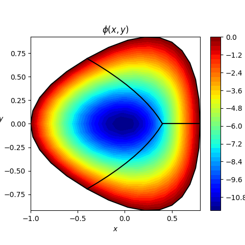
(a)

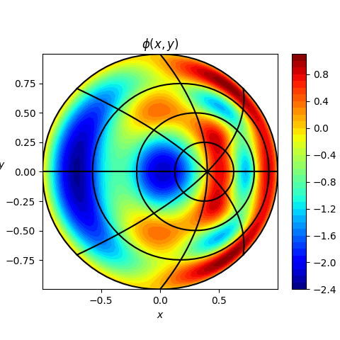
(b)

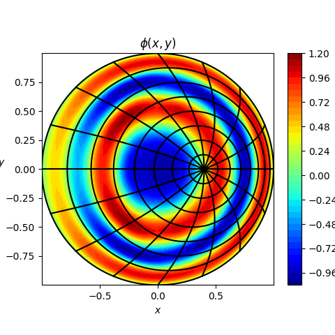
(c)

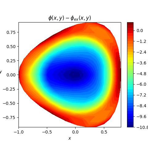
(d)

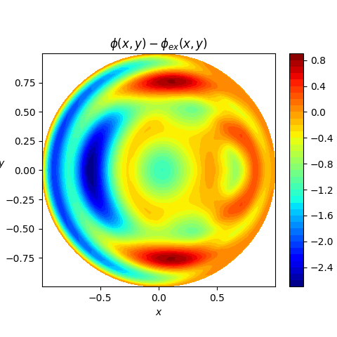
(e)

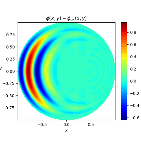
(f)

Figure 1: Poisson problem: approximate solutions $\phi_{h}$ (top) and errors $\phi_{h}-\phi$ (bottom) on the discrete domains $\Omega_{h}$. The mapped cells defined by the spline breaking points are shown as solid lines on the top plots, clearly showing the pole ${\boldsymbol{x}}_{0}=(D,0)$.

To further assess the accuracy of the approximations we next perform a numerical convergence analysis, where we compare three different methods:

• the first one is a conforming discretization, where we approximate the Poisson problem by a standard Galerkin projection in the $C^{1}$ space $U^{0}_{h}$, using the polar spline basis introduced in [8]

• the second one is a $C^{0}$ broken-FEEC discretization, where the problem is solved in the non-conforming space $W^{0}_{h}$ and the $C^{0}$ projection $P^{0}_{V}$ is used to handle the polar singularity

• the third one is a $C^{1}$ broken-FEEC discretization, where the problem is solved again in the non-conforming space $W^{0}_{h}$, but now using the $C^{1}$ projection $P^{0}_{U}$ to handle the polar singularity.

In each case the matrix systems are solved using the conjugate gradient method with a tolerance on the residual error of 1e-12. For each method we measure the relative errors in $L^{2}$ and $H^{1}$ norms,

$$\mathcal{E}_{h,L^{2}}=\frac{\lVert\Pi^{0}_{W}\phi-\phi_{h}\rVert_{L^{2}(\Omega_{h})}}{\lVert\Pi^{0}_{W}\phi\rVert_{L^{2}(\Omega_{h})}},\qquad\mathcal{E}_{h,H^{1}}=\frac{\lVert\Pi^{0}_{W}\phi-\phi_{h}\rVert_{H^{1}(\Omega_{h})}}{\lVert\Pi^{0}_{W}\phi\rVert_{H^{1}(\Omega_{h})}},$$ (117)

for various degrees and grid resolutions. Here we remind that $\Pi^{0}_{W}$ is the spline interpolation operator associated with the space $W^{0}_{h}$, so that $\Pi^{0}_{W}\phi$ may be considered a discrete reference solution on the computational domain $\Omega_{h}$.

In Figure 2 we plot the $L^{2}$ and $H^{1}$ errors for the different discretization methods against increasing mesh resolutions, for several degrees $p=2,\dots 5$. For both norms we find that the three methods yield the same errors: for the conforming and $C^{1}$ broken-FEEC methods this is expected since both solutions should coincide [14], and for the $C^{0}$ broken-FEEC method (a priori more accurate since the solution is computed in a larger space) we see that the additional smoothness constraint on the pole does not degrade the accuracy, which is not surprising here given the high smoothness of the solution. In Table 1 we finally show the convergence rates measured from the errors on the two finest grids: they are found to be close or higher than the standard optimal rates of $p+1$ for the $L^{2}$ norm and $p$ for the $H^{1}$ norm.

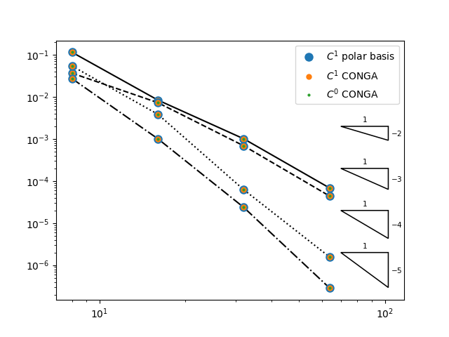
(a) relative $L^{2}$ errors

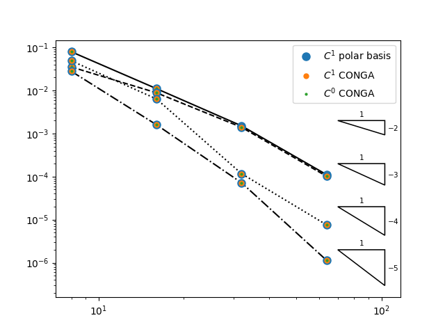
(b) relative $H^{1}$ errors

Figure 2: Poisson problem: relative errors (117) in $L^{2}$ norm (left) and $H^{1}$ norm (right) are plotted for the three different methods described in the text ($C^{1}$ conforming, $C^{0}$ broken-FEEC and $C^{1}$ broken-FEEC) as a function of $N_{s}$ the number of cells along $s$ (with $N_{\theta}=2N_{s}$), represented in abscissa. For each method different spline degrees are used, indicated by different line styles, namely $p=2,3,4,5$ indicated by solid, dashed, dotted and dash-dotted lines respectively.

degree $p$	2	3	4	5
$L^{2}$ rate	3.89	3.97	5.32	6.37
$H^{1}$ rate	3.77	3.78	3.95	5.99

Table 1: $L^{2}$ and $H^{1}$ convergence rates measured from the two finer grids in the error curves plotted in Figure 2.

7.2 Maxwell’s equations

We next apply our approach to the time dependent Maxwell equation (11). Associated with a leap-frog time scheme, the broken-FEEC discretization (12) with regularized mass matrices (77) reads

$$\left\{\begin{array}[]{rl}{\boldsymbol{\mathsf{B}}}^{n+\frac{1}{2}}&={\boldsymbol{\mathsf{B}}}^{n}-\frac{\Delta t}{2}\bbol{C}\bbol{P}^{1}{\boldsymbol{\mathsf{E}}}^{n}\\ \tilde{\bbol{M}}^{1}{\boldsymbol{\mathsf{E}}}^{n+1}&=\tilde{\bbol{M}}^{1}{\boldsymbol{\mathsf{E}}}^{n}+\Delta t\big{(}(\bbol{C}\bbol{P}^{1})^{T}\tilde{\bbol{M}}^{2}{\boldsymbol{\mathsf{B}}}^{n+\frac{1}{2}}-(\bbol{P}^{1})^{T}{\boldsymbol{\mathsf{J}}}^{n+\frac{1}{2}}\big{)}\\ {\boldsymbol{\mathsf{B}}}^{n+1}&={\boldsymbol{\mathsf{B}}}^{n+\frac{1}{2}}-\frac{\Delta t}{2}\bbol{C}\bbol{P}^{1}{\boldsymbol{\mathsf{E}}}^{n+1}\end{array}\right.$$ (118)

with a current source array defined as ${\boldsymbol{\mathsf{J}}}^{n+\frac{1}{2}}_{\mu}=\frac{1}{\Delta t}\int_{t^{n}}^{t^{n+1}}\langle{\boldsymbol{J}}(t),\Lambda^{1}_{\mu}\rangle\,\mathrm{d}t$, see [20].

To assess the qualitative properties of our polar broken-FEEC scheme, we consider a circular wave propagating from the center ${\boldsymbol{x}}_{C}=(0,0)$ through the pole ${\boldsymbol{x}}_{0}=(D,0)$. The initial condition is a Gaussian pulse centered at the disk origin

$${\boldsymbol{E}}(t=0,{\boldsymbol{x}})=\begin{pmatrix}y\\ -x\end{pmatrix}\exp\Big{(}-\frac{\lVert{\boldsymbol{x}}\rVert^{2}_{2}}{2\sigma^{2}}\Big{)},\quad B(t=0,{\boldsymbol{x}})=\operatorname{{curl}}{\boldsymbol{E}}^{0}({\boldsymbol{x}})\qquad\text{for ${\boldsymbol{x}}=(x,y)\in\mathbb{R}^{2}$},$$ (119)

with $\sigma=0.1$. In Figure 3 we plot the profiles of the (scalar) transverse magnetic field $B_{z}$ at different times, for increasing resolutions: while spurious oscillations can be seen around the pole on the coarsest mesh, they quickly disappear as the resolution is increased.

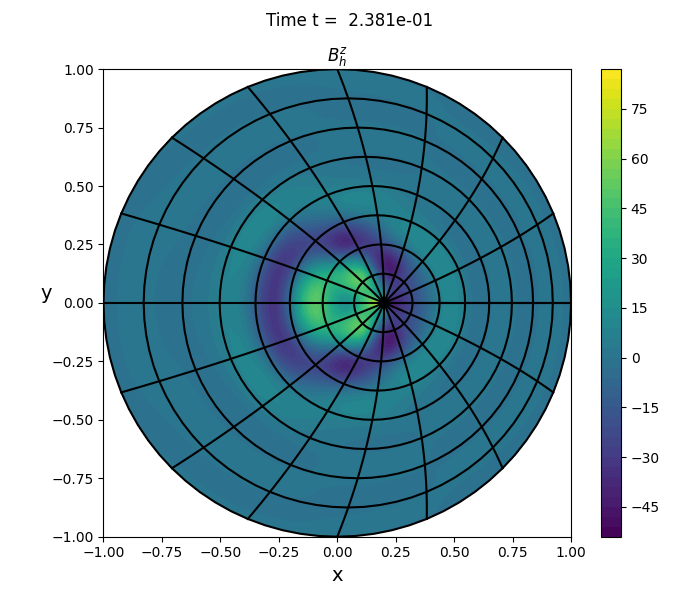
(a)

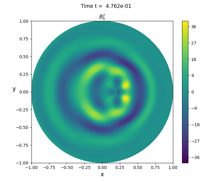
(b)

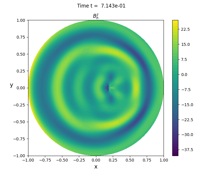
(c)

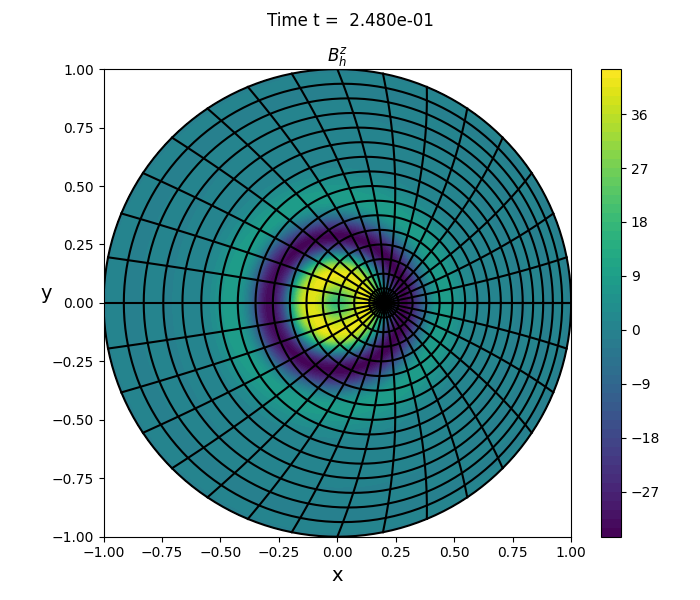
(d)

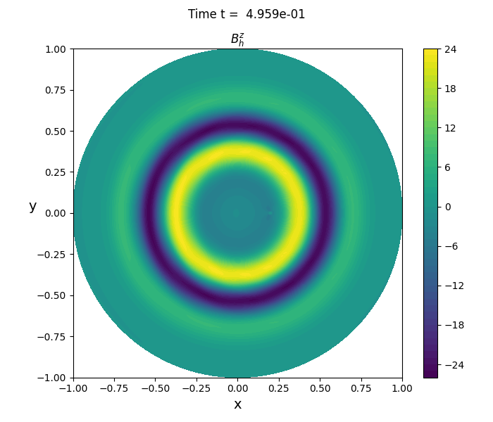
(e)

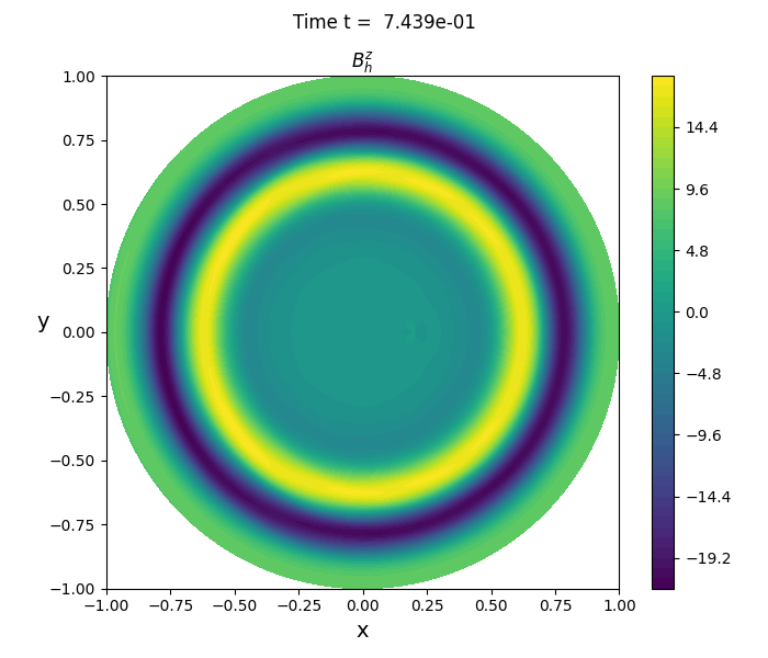
(f)

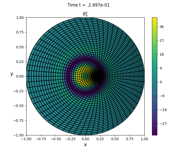
(g)

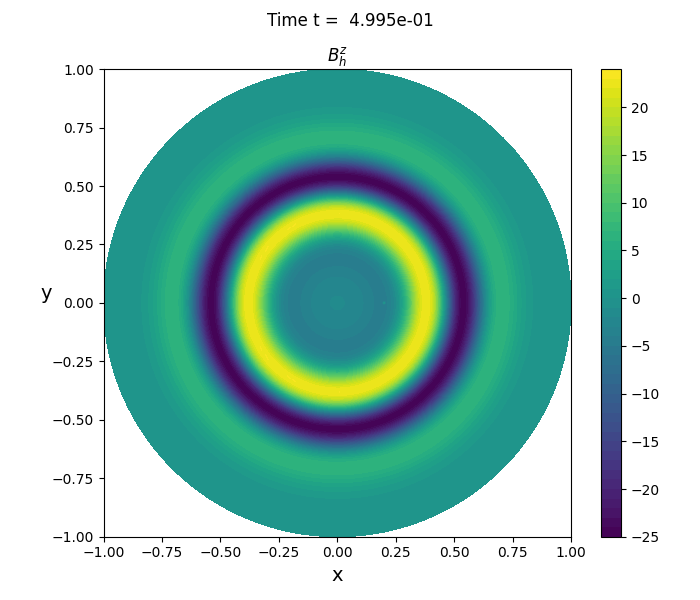
(h)

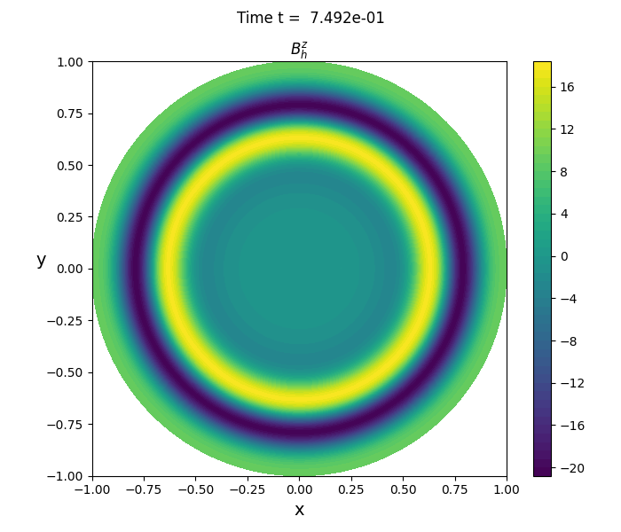
(i)

Figure 3: Maxwell equations: propagation of a circular wave at three successive times ($t\approx 2.5,5$ and $7.5$, from left to right) computed with the $C^{1}$ broken-FEEC scheme (118). Three grids (represented on the left plots) are used, with $N_{s}=8$, $16$ and $32$ cells along $s$, and $N_{\theta}=2N_{s}$ along the periodic variable (from top to bottom).

Finally we assess the quantitative convergence of our broken-FEEC Maxwell solver with a time-harmonic solution of Bessel-Fourier type, with mode $(n,m)\in\mathbb{N}^{2}$. Let us remind how this solution is obtained. Using the (standard) polar parametrisation $F_{D=0}:(s,\theta)\mapsto(x,y)=(s\cos\theta,s\sin\theta)$ of the disk domain (112), the complex solution can be expressed as the pushforward

$$B=\mathcal{F}^{2}{\hat{B}},\qquad{\boldsymbol{E}}=\mathcal{F}^{1}{\hat{\boldsymbol{E}}}$$ (120)

of logical fields of the form

$${\hat{B}}(t,s,\theta)=se^{i\omega t}J_{n}(ks)\cos(n\theta),\qquad{\hat{\boldsymbol{E}}}(t,s,\theta)=\begin{pmatrix}E_{s}(t,s,\theta)\\ E_{\theta}(t,s,\theta)\end{pmatrix}=ie^{i\omega t}\begin{pmatrix}\frac{n}{ks}J_{n}(ks)\sin(n\theta)\\ sJ^{\prime}_{n}(ks)\cos(n\theta)\end{pmatrix}$$ (121)

where $J_{n}$ is the Bessel function of the first kind and $k=\omega=j^{\prime}_{n,m}$ is the $m$-th root of its derivative $J^{\prime}_{n}$.

Here, one easily verifies that the logical fields satisfy $\partial_{t}{\hat{B}}+\operatorname{\widehat{curl}}{\hat{\boldsymbol{E}}}=0$, so that Faraday’s equation follows from the commuting properties of the pushforward operators, namely (100) (note that $E_{\theta}(s=0)=0$). To verify that Ampère’s equation holds as well, one can use the explicit forms of the pushforward operators (31) to rewrite (120)–(121) as

$$\begin{cases}B(t,x,y)=\frac{1}{s}{\hat{B}}(t,s,\theta)=e^{i\omega t}J_{n}(ks)\cos(n\theta)\\[5.0pt] {\boldsymbol{E}}(t,x,y)=\begin{pmatrix}\cos\theta&-\frac{1}{s}\sin\theta\\ \sin\theta&\frac{1}{s}\cos\theta\end{pmatrix}{\hat{\boldsymbol{E}}}(t,s,\theta)=ie^{i\omega t}\begin{pmatrix}\frac{n}{ks}J_{n}(ks)\sin(n\theta)\cos\theta-J^{\prime}_{n}(ks)\cos(n\theta)\sin\theta\\ \frac{n}{ks}J_{n}(ks)\sin(n\theta)\sin\theta+J^{\prime}_{n}(ks)\cos(n\theta)\cos\theta\end{pmatrix},\end{cases}$$

and the fact that $J_{n}$ is the (bounded) solution of the differential equation

$$x^{2}J^{\prime\prime}_{n}(x)+xJ^{\prime}_{n}(x)+(x^{2}-n^{2})J_{n}(x)=0.$$ (122)

We remind that close to $s\to 0$ we have $J_{n}(ks)\sim\big{(}\frac{ks}{2}\big{)}^{n}/\Gamma(n+1)$, see [21], so that ${\boldsymbol{E}}$ has no singularity at the pole. The homogeneous boundary condition ${\boldsymbol{n}}\times{\boldsymbol{E}}=0$ is easily verified using $E_{\theta}(s=1)=0$ which follows from the fact that $J^{\prime}_{n}(k)=0$.

In our numerical convergence study we consider the real part of the above Bessel-Fourier solution with mode number $(m,n)=(2,3)$, on a time range $[0,T]$ with $T=0.1$. The initial solutions are represented in Figure 4, and in Figure 5 we plot the errors of our broken-FEEC scheme (118) at $t=T$, with $C^{0}$ and $C^{1}$ projection operators, i.e. using $P^{1}=P^{1}_{V}$ and $P^{1}_{U}$ respectively. Note that in our experiments a Suzuki-Yoshida [22, 23] time scheme of order 4 is obtained by composing the Strang steps as described in [4, Sec. 5.2].

Again, we observe that the $C^{0}$ and $C^{1}$ schemes yield virtually the same errors, except in a couple of cases for which we do not have a clear diagnostic. As for the convergence rates (measured again using the finest grids, and displayed in Table 2), they are close to $p$ which may be considered as optimal given that the logical approximation spaces $\hat{W}^{1}_{h}$ and $\hat{W}^{2}_{h}$ consist of B-splines of mixed degree $p$ and $p-1$, see (28).

degree $p$	2	3	4	5
${\boldsymbol{E}}$ error rate	2.02	3.05	4.08	5.14
$B$ error rate	2.05	3.16	4.20	4.99

Table 2: Convergence rates for the errors in ${\boldsymbol{E}}$ and $B$ as computed with the $C^{1}$ broken-FEEC scheme (118), measured from the two finer grids in the error curves plotted in Figure 5.

Overall these numerical experiments confirm the ability of our broken-FEEC approach to approximate problems on polar domains.

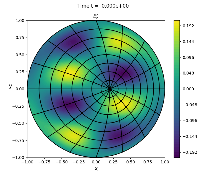
(a)

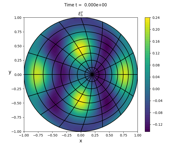
(b)

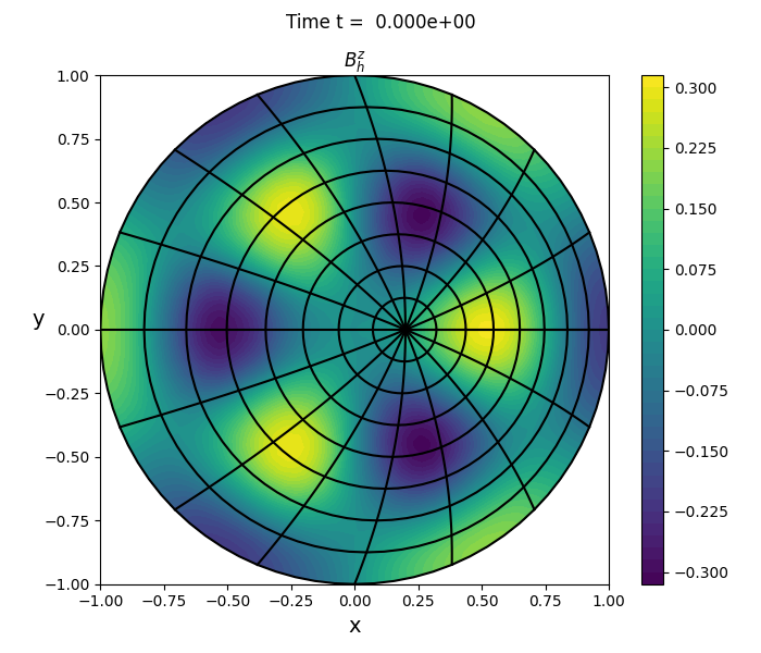
(c)

Figure 4: Initial Bessel-Fourier solution (from left to right: $E_{x}$, $E_{y}$, $B$) with mode number $(m,n)=(2,3)$ used for the convergence study of Maxwell’s equations.

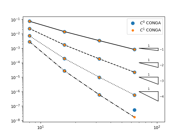
(a)

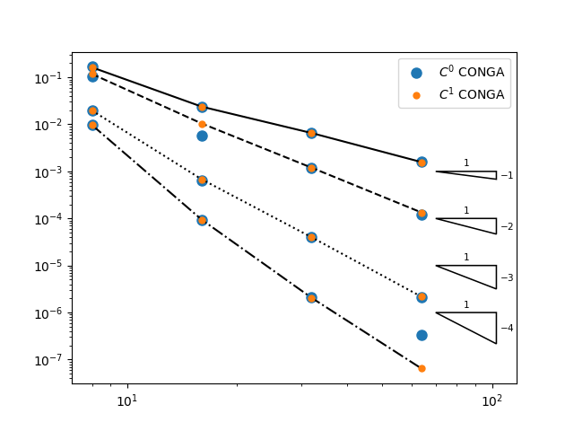
(b)

Figure 5: Maxwell’s equations: relative $L^{2}$ errors for the ${\boldsymbol{E}}$ (left) and $B$ fields (right) obtained using the polar broken-FEEC scheme (118) with $C^{0}$ and $C^{1}$ projection operators $P^{1}=P^{1}_{V}$ and $P^{1}_{U}$. As in Figure 2, errors are plotted versus $N_{s}$ the number of cells along $s$ (with $N_{\theta}=2N_{s}$) and different spline degrees ($p=2,3,4,5$) are used, indicated by different line styles (solid, dashed, dotted and dash-dotted lines respectively).

Appendix A Reminder on B- and M-splines

The splines $B_{i}(s)$ and $\mathring{B}_{j}(\theta)$ involved in this article correspond to the normalized B-splines, namely $B_{i}(s)=(s_{i+m}-s_{i})Q^{m}_{i}(s)$ with $m=p+1$ in Schumaker’s notation [24]. We further denote $M_{i}(s)\coloneqq(m-1)Q^{m-1}_{i+1}(s)$ for $0\leq i<n_{s}-1$, yielding the derivative formula

$$B_{i}^{\prime}=M_{i-1}-M_{i}\quad\text{ for }\quad 0\leq i<n_{s}$$ (123)

where we have set $M_{-1}\coloneqq M_{n_{s}-1}\coloneqq 0$ for convenience. We remind that B-splines satisfy a partition of unity property, namely

$$\sum_{i=0}^{n_{s}-1}B_{i}(s)=1,\qquad\sum_{j=0}^{n_{\theta}-1}\mathring{B}_{j}(\theta)=1$$ (124)

hold for all $s$ and $\theta$, and that those defined from open knot sequences are interpolatory at the end points. In particular, we have

$$B_{i}(0)=M_{i}(0)=0\text{ for }i>0,\quad B_{0}(0)=1,\quad$$ (125)

and

$$B^{\prime}_{i}(0)=0\text{ for }i>1,\quad B_{1}^{\prime}(0)=M_{0}(0)=\frac{p}{s_{p+1}}.$$ (126)

A standard relation follows from (123) and (125)–(126), namely

$$\int_{0}^{L}M_{i}(s)\,\mathrm{d}s=1\qquad\text{ for }\quad 0\leq i<n_{s}-1.$$ (127)

For the periodic splines along $\theta$ we define similarly $\mathring{M}_{j}(\theta)\coloneqq(m-1)\mathring{Q}^{m-1}_{j+1}(\theta)$, yielding the same derivative formula than aboove,

$$\mathring{B}_{j}^{\prime}=\mathring{M}_{j-1}-\mathring{M}_{j}\quad\text{ for }\quad 0\leq j<n_{s}$$ (128)

where we now observe that every spline $\mathring{M}_{j}$ is defined by periodicity. With regular knots the periodic M-splines also sum to a constant value, namely

$$\sum_{j=0}^{n_{\theta}-1}\mathring{M}_{j}(\theta)=\frac{1}{\Delta\theta}\quad\text{ with }~~\Delta\theta=\frac{2\pi}{n_{\theta}}.$$ (129)

Note that with this definition the splines $\mathring{B}_{j}(\theta)$ and $\mathring{M}_{j}(\theta)$ are supported in the respective intervals $[\theta_{j},\theta_{j+p+1}]$ and $[\theta_{j+1},\theta_{j+p+1}]$, in particular we have

$$\mathring{B}_{j}\mathring{M}_{j+k}=0\quad\text{ for }\quad k\notin\{-p,\dots p-1\}.$$ (130)

We further list some elementary relations satisfied by the regular angles $\theta_{j}=\frac{2\pi j}{n_{\theta}}$, which hold as long as $n_{\theta}=4n^{\prime}$ for a positive integer $n^{\prime}>0$, see Assumption 2.2:

$$\begin{array}[]{c}\displaystyle\sum_{j=0}^{n_{\theta}-1}\cos(2\theta_{j})=\sum_{j=0}^{n_{\theta}-1}\cos(\theta_{j})=\sum_{j=0}^{n_{\theta}-1}\sin(2\theta_{j})=\sum_{j=0}^{n_{\theta}-1}\sin(\theta_{j})=0\\ \\ \displaystyle\sum_{j=0}^{n_{\theta}-1}2\cos^{2}\theta_{j}=\sum_{j=0}^{n_{\theta}-1}(1+\cos(2\theta_{j}))=\sum_{j=0}^{n_{\theta}-1}2\sin^{2}\theta_{j}=\sum_{j}(1-\cos(2\theta_{j}))=n_{\theta}\\ \\ \displaystyle\sum_{j=0}^{n_{\theta}-1}2\cos\theta_{j}\cos(\theta_{j}-\theta_{k})=n_{\theta}\cos\theta_{k},\qquad\sum_{j=0}^{n_{\theta}-1}2\sin\theta_{j}\cos(\theta_{j}-\theta_{k})=n_{\theta}\sin\theta_{k}~.\end{array}$$ (131)

References

- \bibcommenthead
- Bossavit [1998] Bossavit, A.: Computational Electromagnetism: Variational Formulations, Complementarity, Edge Elements. Academic Press. Academic Press, ??? (1998). https://app.readcube.com/library/8de573ae-13bf-4887-8bf5-8d9936dd78d5/item/bd6384b4-c9d7-4e49-a6e6-f19b3537c219
- Hiptmair [2002] Hiptmair, R.: Finite elements in computational electromagnetism. Acta Numerica 11, 237–339 (2002)
- Arnold et al. [2006] Arnold, D.N., Falk, R.S., Winther, R.: Finite element exterior calculus, homological techniques, and applications. Acta Numerica 15, 1–155 (2006) https://doi.org/10.1017/S0962492906210018 . Publisher: Cambridge University Press. Accessed 2023-03-17
- Kraus et al. [2017] Kraus, M., Kormann, K., Morrison, P.J., Sonnendruecker, E.: GEMPIC: geometric electromagnetic particle-in-cell methods. Journal of Plasma Physics 83(04) (2017) https://doi.org/%****␣numapolaconga.bbl␣Line␣100␣****10.1017/s002237781700040x
- Campos Pinto et al. [2022] Campos Pinto, M., Kormann, K., Sonnendrücker, E.: Variational Framework for Structure-Preserving Electromagnetic Particle-in-Cell Methods. Journal of Scientific Computing 91(2), 46 (2022) https://doi.org/10.1007/s10915-022-01781-3 . Accessed 2023-01-30
- Perse et al. [2021] Perse, B., Kormann, K., Sonnendrücker, E.: Geometric Particle-in-Cell Simulations of the Vlasov–Maxwell System in Curvilinear Coordinates. SIAM Journal on Scientific Computing 43(1), 194–218 (2021) https://doi.org/10.1137/20M1311934 . Publisher: Society for Industrial and Applied Mathematics. Accessed 2025-01-18
- Buffa et al. [2011] Buffa, A., Rivas, J., Sangalli, G., Vázquez, R.: Isogeometric discrete differential forms in three dimensions. SIAM Journal on Numerical Analysis 49(2), 818–844 (2011) https://doi.org/10.1137/100786708
- Toshniwal et al. [2017] Toshniwal, D., Speleers, H., Hiemstra, R.R., Hughes, T.J.R.: Multi-degree smooth polar splines: a framework for geometric modeling and isogeometric analysis. Comput. Methods Appl. Mech. Engrg. 316, 1005–1061 (2017) https://doi.org/10.1016/j.cma.2016.11.009
- Speleers and Toshniwal [2021] Speleers, H., Toshniwal, D.: A general class of smooth rational splines: application to construction of exact ellipses and ellipsoids. Comput.-Aided Des. 132, 102982–14 (2021) https://doi.org/10.1016/j.cad.2020.102982
- Toshniwal and Hughes [2021] Toshniwal, D., Hughes, T.J.R.: Isogeometric discrete differential forms: non-uniform degrees, Bézier extraction, polar splines and flows on surfaces. Comput. Methods Appl. Mech. Engrg. 376, 113576–44 (2021) https://doi.org/10.1016/j.cma.2020.113576
- Patrizi and Toshniwal [2025] Patrizi, F., Toshniwal, D.: Isogeometric de Rham complex discretization in solid toroidal domains. arXiv. arXiv:2106.10470 [math] (2025). https://doi.org/10.48550/arXiv.2106.10470 . http://arxiv.org/abs/2106.10470 Accessed 2025-01-16
- Holderied and Possanner [2022] Holderied, F., Possanner, S.: Magneto-hydrodynamic eigenvalue solver for axisymmetric equilibria based on smooth polar splines. Journal of Computational Physics 464, 111329 (2022) https://doi.org/10.1016/j.jcp.2022.111329 . Accessed 2025-01-15
- Campos Pinto and Sonnendrücker [2016] Campos Pinto, M., Sonnendrücker, E.: Gauss-compatible Galerkin schemes for time-dependent Maxwell equations. Mathematics of Computation 85(302), 2651–2685 (2016) https://doi.org/10.1090/mcom/3079 . Accessed 2023-04-19
- Güçlü et al. [2023] Güçlü, Y., Hadjout, S., Campos Pinto, M.: A Broken FEEC Framework for Electromagnetic Problems on Mapped Multipatch Domains. Journal of Scientific Computing 97(2), 52 (2023) https://doi.org/10.1007/s10915-023-02351-x . Accessed 2023-10-19
- Kreeft et al. [2011] Kreeft, J., Palha, A., Gerritsma, M.: Mimetic framework on curvilinear quadrilaterals of arbitrary order (2011)
- Bochev and Hyman [2006] Bochev, P.B., Hyman, J.M.: Principles of mimetic discretizations of differential operators. In: Compatible Spatial Discretizations. Papers Presented at IMA Hot Topics Workshop: Compatible Spatial Discretizations for Partial Differential Equations, Minneapolis, MN, USA, May 11–15, 2004., pp. 89–119. New York, NY: Springer, ??? (2006)
- Gerritsma [2011] Gerritsma, M.: Edge functions for spectral element methods. In: Spectral and High Order Methods for Partial Differential Equations, pp. 199–207. Springer, ??? (2011)
- Lewis and Bellan [1990] Lewis, H.R., Bellan, P.M.: Physical constraints on the coefficients of Fourier expansions in cylindrical coordinates. Journal of Mathematical Physics 31(11), 2592–2596 (1990) https://doi.org/10.1063/1.529009 . _eprint: https://pubs.aip.org/aip/jmp/article-pdf/31/11/2592/19139813/2592_1_online.pdf
- Robidoux [2008] Robidoux, N.: Polynomial histopolation, superconvergent degrees of freedom and pseudo-spectral discrete Hodge operators. Unpublished (2008). http://www.cs.laurentian.ca/nrobidoux/prints/super/histogram.pdf
- Campos Pinto and Sonnendrücker [2017] Campos Pinto, M., Sonnendrücker, E.: Compatible Maxwell solvers with particles II: conforming and non-conforming 2D schemes with a strong Faraday law. The SMAI Journal of computational mathematics 3, 91–116 (2017) https://doi.org/10.5802/smai-jcm.21 . Accessed 2025-01-07
- Abramowitz and Stegun [1964] Abramowitz, M., Stegun, I.A.: Handbook of Mathematical Functions with Formulas, Graphs, and Mathematical Tables. U.S. Government Printing Office, Washington, D.C., vol. 55. U.S. Government Printing Office, Washington, D.C., ??? (1964). https://app.readcube.com/library/8de573ae-13bf-4887-8bf5-8d9936dd78d5/item/25808fc4-9deb-4838-b396-e72d6b174662
- Suzuki [1990] Suzuki, M.: Fractal decomposition of exponential operators with applications to many-body theories and Monte Carlo simulations. Physics Letters A 146(6), 319–323 (1990) https://doi.org/10.1016/0375-9601(90)90962-N . Accessed 2025-01-11
- Yoshida [1990] Yoshida, H.: Construction of higher order symplectic integrators. Physics Letters A 150(5), 262–268 (1990) https://doi.org/10.1016/0375-9601(90)90092-3 . Accessed 2025-01-11
- Schuma er [2007] Schuma er, L.L.: Spline Functions: Basic Theory, 3rd edn. Cambridge Mathematical Library, p. 582. Cambridge University Press, Cambridge, ??? (2007). https://doi.org/10.1017/CBO9780511618994 . https://doi.org/10.1017/CBO9780511618994