Interpretation of run-and-tumble motion as jump-process: the case of a harmonic trap

Abstract

By mapping run-and-tumble motion onto jump-process (a process in which a particle, instead of moving continuously in time, performs consequential jumps), a system in a steady-state can be formulated as an integral equation. The key ingredient of this formulation is the transition operator $G(x,x^{\prime})$, representing the probability distribution of jumps along the $x$-axis for a particle located at $x^{\prime}$ before a jump. For particles in a harmonic trap, exact expressions for $G(x,x^{\prime})$ are obtained and, in principle, $G(x,x^{\prime})$ has all the information about a stationary distribution $\rho(x)$. One way to extract $\rho$ is to use the condition of stationarity, $\rho(x)=\int dx^{\prime}\,\rho(x^{\prime})G(x,x^{\prime})$, resulting in an integral equation formulation of the problem. For the system in dimension $d=2$, there is an unexpected reduction of complexity; the expression for $G(x,x^{\prime})$ is found to be reversible, which implies that $\rho(x)$ (within the jump-process interpretation) obeys the detailed balance condition, and $\rho$ can be obtained from the detailed balance relation, $\rho(x^{\prime})G(x,x^{\prime})=\rho(x)G(x^{\prime},x)$.

I Introduction

Distinguishing feature of self-propelled motion is its continuous use of energy, which is dissipated into an environment without being recovered. This leads to the breakdown of the fluctuation-dissipation relation and the detailed-balance condition, resulting in non-equilibrium statistical mechanics. Run-and-tumble particle model (RTP) is the simplest and most ideal representation of self-propelled motion Tailleur and Cates (2008, 2009); Grognot and Taute (2021); Malakar et al. (2018); Razin (2020). It was originally conceived to represent motion of a bacteria Berg (1983); Schnitzer (1993). Other popular models of self-propelled particles, not considered in this work, are the active Brownian particle model Romanczuk et al. (2012); Fily and Marchetti (2012); Marchetti et al. (2013); Maggi et al. (2015); Solon et al. (2015a); Étienne Fodor and Cristina Marchetti (2018); Shankar and Marchetti (2018); Das et al. (2018); Caraglio and Franosch (2022); Nakul and Gopalakrishnan (2023); Caporusso et al. (2023); Semeraro et al. (2024); Caporusso et al. (2024), more appropriate for representing active colloids Archer and Ebbens , and the active Ornstein-Uhlenbeck particle model Szamel (2014); Martin et al. (2021); Caprini et al. (2019); Semeraro et al. (2023), originally conceived to represent passive particles in an active bath. Alternatively, an active motion can be induced when passive particles are agitated by constantly fluctuating external potential Pal and Sabhapandit (2013); Santra et al. (2021); Gupta et al. (2020, 2021); Alston et al. (2022); Biroli et al. (2024); Frydel (2024a).

RTP motion consists of two alternating stages. During the deterministic "run" stage, a particle moves at constant swimming velocity in a fixed orientation, and during the "tumble" stage, which occurs instantaneously, a particle changes its orientation. The duration of the "run" stage is drawn from an exponential distribution $p_{t}$, which also implies that tumbling events occur at a constant rate. Any other functional form of $p_{t}$ implies a non-constant rate of tumbling, which could be represented by a position dependent rate Farago and Smith (2024).

RTP model in one-dimension has been extensively analyzed in Malakar et al. (2018). The entropy production rate was considered in Razin (2020); Frydel (2022a); Padmanabha et al. (2023). Dynamic properties, including first passage, survival probability, and local time were studied in Angelani et al. (2014); Mori et al. (2020); Bruyne et al. (2021); Singh and Kundu (2021). Extensions of the RTP model in one-dimension to include more than two discrete swimming orientations were considered in Basu et al. (2020); Frydel (2021, 2022b); Breoni et al. (2022). A harmonic potential in one-dimension was considered in Tailleur and Cates (2008, 2009); Basu et al. (2020); Frydel (2022c); Smith et al. (2022); Smith and Farago (2022); Frydel (2023a). RTP particles in other types of potentials and under different conditions has been considered in Dhar et al. (2019); Farago and Smith (2024); Roberts and Zhen (2023); Dhar et al. (2019); Doussal et al. (2020); de Pirey and van Wijland (2023); Angelani (2015); Bressloff (2023); Woillez et al. (2019); Detcheverry (2015); Dean et al. (2021); Angelani (2017).

In this work, we revisit the system of RTP particles in a harmonic trap under steady-state conditions within an alternative formulation of the problem. RTP particles in a harmonic trap is a popular system due to its relative analytical tractability. This tractability has to do with the nature of a harmonic potential (or a linear force), which, to some extent, simplifies things. For example, a stationary distribution of any type of self-propelled particles at finite temperature can be represented as a convolution of two well-defined distributions, and as a consequence of the independence of thermal noise and an active motion Frydel (2023b, a, 2024b). As a result, the entropy production rate (in both overdamped and underdamped regime) is independent of temperature and can be calculated exactly for any dimension Frydel (2023b).

As regards stationary distributions of RTP particles in a harmonic trap, an exact expression can be obtained directly from the Fokker-Planck equation (FP) for dimension $d=1$, where swimming orientations have two discrete values. The analysis becomes more challenging for higher dimensions where the orientation of motion is continuous.

For $d=2$, a stationary distribution $\rho$ cannot be obtained directly from the FP equation. However, the FP equation can be used to obtain exact expressions of the moments of $\rho$ Frydel (2023a, 2024b); Dutta et al. (2025). By inference, one can recognize that these moments are related to the moments of $\rho$ in $d=1$, thus, $\rho$ in both $d=1$ or $d=2$ must share the same functional form Frydel (2022c). Apart from this inferential proof, a more rigorous proof is still missing, and one of the aims of this work is to rectify this situation.

For $d=3$, the situation becomes even more complicated. Exact expressions of all moments can be generated from a recurrence relation, but the recurrence relation does not admit of a solution Frydel (2023a). This suggests that $\rho$ has a more complex structure than $\rho$ in $d=1$ and $d=2$. In this work, we revisit the system in $d=3$ within the integral equation formulation for possible insights.

As regards the integral formulation approach, a recent article Frydel (2024b) considered this formulation for a system of RTP particles in slit geometry (particles between two parallel walls). The resulting formulation allowed a greater degree of analytical tractability compared to the more standard FP formulation. Also, the governing equations were found to be the same as those for a splitting probability problem Klinger et al. (2022). (The splitting probability is a probability that a random walker, starting from some point between two walls, arrives at one of the wall without first arriving at the other wall. It correctly represents various physical processes, for example, transport of photons or neutrons in scattering media Rotter and Gigan (2017).)

The integral equation formulation has recently been applied to another statistical-mechanical problem known as stochastic resetting Evans and Majumdar (2011); Masó-Puigdellosas et al. (2019); Singh et al. (2022). The integral in this case is over time rather than space, but the motivation is similar: to find an alternative theoretical description that is more flexible and provides increased analytical tractability over more standard descriptions.

Motivated by recent interest in integral equation formulation of statistical mechanical systems, in this work, we apply this approach to RTP particles in a harmonic trap. The key quantity within this framework is the transition operator $G(x,x^{\prime})$, or the distribution of a particle on the $x$-axis after a single jump (given that before a jump, a particle was at $x^{\prime}$). The stationary distribution $\rho(x)$ is then obtained from the stationarity condition $\rho(x)=\int dx^{\prime}\,\rho(x^{\prime})G(x,x^{\prime})$, giving rise to an integral equation formulation of the problem. As the transition operator $G(x,x^{\prime})$ depends on a system dimension $d$, how the integral equation is analyzed depends on $d$.

This paper is organized as follows. In Sec. (II) we introduce the model. In Sec. (III) we provide justification for the jump-process algorithm. It is determined that the algorithm is valid only if the persistence time $t_{p}$, which determines the duration of a "run" stage, is drawn from an exponential distribution. In Sec. (IV), we provide a general formula for the transition operator $G(x,x^{\prime})$ for particles in a harmonic trap. In Sec. (IV.1), we obtain an exact expression for $G(x,x^{\prime})$ in dimension $d=1$, and the resulting integral equation is solved. In Sec. (IV.2), we repeat the same steps for dimension $d=2$. The transition operator $G(x,x^{\prime})$ in this case is reversible, which implies that $\rho$ satisfies the detailed balance condition. This simplifies the problem and allows us to obtain a simple algebraic expression for $\rho$. In Sec. (IV.3) we consider the case $d=3$.

II The model

RTP motion consists of two alternating stages. During the "run" stage, which is deterministic, a particle moves at a constant swimming velocity $v_{0}$ in a direction designated by the unit vector ${\bf u}$. The duration of the "run" stage is determined by the persistence time $t_{p}$ drawn from the exponential distribution $p_{t}\propto e^{-t_{p}/\tau}$, where $\tau$ represents the average persistence time (exponential $p_{t}$ indicates that tumbling events occur at a constant rate). During the "tumble" stage, which occurs instantaneously, a particle changes its orientation to any other orientation, ${\bf u}\to{\bf u}^{\prime}$. If a particle is trapped in an external potential $u({\bf r})$, there is an additional force ${\bf F}=-\mbox{\boldmath$\nabla$}u$ acting on a particle.

Within the Fokker-Planck formulation, the probability distribution of RTP particles (at zero temperature and for convenience assumed to occur in two-dimensions) evolves as Solon et al. (2015b); Frydel (2021)

$$\frac{\partial n}{\partial t}=-\mbox{\boldmath$\nabla$}\cdot\left[\left({\bf F}+v_{0}{\bf u}\right)n\right]-\frac{1}{\tau}\left(n-\frac{1}{2\pi}\int_{0}^{2\pi}d\theta\,n({\bf r},\theta,t)\right),$$ (1)

where $n\equiv n({\bf r},\theta,t)$ is the probability distribution. The first term on the right-hand side is connected to the flux, and the second term governs the evolution of a unit vector ${\bf u}=(\cos\theta,\sin\theta)$ representing the swimming orientation in two-dimensions, whereby it gives rise to active motion. (In Appendix (A) we write down Fokker-Planck equations for dimensions $d=1,3$.)

In this work, we consider RTP particles confined to a harmonic potential in one direction, $u(x)=\frac{K}{2}x^{2}$. And because a stationary distribution of such a system is non-uniform along the $x$-axis only, the system is effectively one-dimensional. The projected swimming velocity on the $x$-axis, $v=v_{0}\cos\theta$, results in a probability distribution $p_{v}(v)$ whose distribution within the interval $v\in[-v_{0},v_{0}]$ depends on a system dimension.

The Fokker-Planck equation of such a system can be represented as

$$0=\left(\mu Kx-v\right)n^{\prime}-\frac{1}{\tau}\left(n-\int_{-v_{0}}^{v_{0}}dv\,p_{v}n\right),$$ (2)

where $n\equiv n(x,v)$ is the time-independent density distribution. Note that by transforming Eq. (1) to Eq. (2), an integral over $\theta$ transforms to an integral over $v$ as a result of a change of a variable $v=v_{0}\cos\theta$. The advantage of the formulation in Eq. (2) is that it applies to all dimensions. The dependence on a system dimension enters via $p_{v}(v)$,

$$p_{v}=\frac{1}{2}\begin{cases}\delta(v-v_{0})+\delta(v+v_{0}),&\text{for $d=1$},\\ \frac{2}{\pi}\frac{1}{\sqrt{v_{0}^{2}-v^{2}}},&\text{for $d=2$},\\ \frac{1}{v_{0}},&\text{for $d=3$}.\\ \end{cases}$$ (3)

For $d=1$ there are only two possible orientations of motion, $v=\pm v_{0}$, and so the distribution is represented by two delta functions Razin (2020). The distributions for $d=2$ and $d=3$ are obtained using the change of a variable $v=v_{0}\cos\theta$ that modifies the integral over an angular orientation as

$$\int_{0}^{2\pi}d\theta~\to~=\int_{-v_{0}}^{v_{0}}dv\,\frac{1}{\sqrt{v_{0}^{2}-v^{2}}}$$

for $d=2$, and

$$\int_{0}^{2\pi}d\phi\int_{0}^{\pi}d\theta\,\sin\theta~\to~\int_{-v_{0}}^{v_{0}}dv$$

for $d=3$. A marginal stationary distribution is defined as

$$\rho(x)=\int_{-v_{0}}^{v_{0}}dv\,p_{v}(v)n(x,v).$$ (4)

In Appendix (B) we provide more details of the two transformations.

In this work, we re-formulate the problem of RTP particles in a stationary state as an integral equation involving $\rho(x)$ rather than $n(x,v)$ as it appears in the FP formulation in Eq. (2). This means that we will not analyze Eq. (2). Instead, we will analyze an alternative formulation of the same system. We obtain such a re-formulation by re-interpreting the RTP motion as a jump-process, the details of which we provide in the next section.

III jump-process sampling method

In this work, jump-process refers to a sampling algorithm wherein particle positions are sampled at a "tumble" stage only; all configurations generated during a "run" stage are neglected. Because of this, a particle appears to be jumping rather than moving continuously in time. Despite the incomplete sampling, it was observed that the algorithm recovers correct stationary distributions Frydel (2024b). Such re-interpretation of the RTP motion as a jumping process, led to an alternative formulation of the problem (as an integral equation) of RTP particles in a slit geometry that permitted the calculation of stationary distributions Frydel (2024b).

In this work, we apply the same technique to a system of RTP particles in a harmonic trap. Before proceeding, however, we discuss the jump-process algorithm in more detail.

III.1 simulations

The restriction of sampling to "tumble" events, on the one hand, can be regarded as an alternative algorithm for obtaining a stationary distribution or, on the other hand, as a method for calculating a distribution of tumbling events in space (rather than an actual distribution of particles). The two distributions (of particles and of tumbling events in space) are identical if the duration of a "run" stage $t_{p}$ is drawn from an exponential probability distribution, $p_{t}=\tau^{-1}e^{-t_{p}/\tau}$. The reason for this special status of an exponential distribution is that it represents a constant rate process. As a consequence, the number of tumbling events at a particular position is proportional to the number of particles at that position. Since this is not true for non-exponential $p_{t}$, the jump-process method in those cases does not yield correct $\rho(x)$.

In Fig. (1) we compare stationary distributions $\rho(x)$ of RTP particles between two parallel walls generated by (i) the jump-process (represented by red points) and (ii) continuous time algorithm (represented by black lines). The two algorithms yield the same distributions if $p_{t}$ is exponential (the left-hand-side plot). For a uniform $p_{t}$, the two algorithms yield different distributions (the right-hand-side plot). Note that none of the distributions in Fig. (1) are normalized to one, since there is a fraction of particles adsorbed at a wall (represented by delta functions, not shown in the figure). The fact that a distribution for a uniform $p_{t}$ obtained from the jump-process is always below the correct distribution implies that tumbling is more frequent for adsorbed particles.

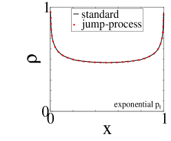
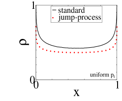
Figure 1: Stationary distributions of RTP particles between two parallel walls in 3D obtained from the standard and jump-process algorithms. The system parameters are $L=\tau=v_{0}=1$. The results are for an exponential and uniform $p_{t}$, $p_{t}=\tau^{-1}e^{-t/\tau}$ and $p_{t}=(2\tau)^{-1}\Theta(2\tau-t)$, respectively. The distribution $p_{v}$ corresponds to the distribution for $d=3$ in Eq. (3).

In Fig. (2), we show similar plots for RTP particles in a harmonic trap. As in the previous figure, the jump-process algorithm yields incorrect $\rho$ if $p_{t}$ is non-exponential.

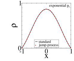
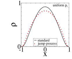
Figure 2: An analogous figure to that in Fig. (1), but for RTP particles trapped in a harmonic potential $u(x)=Kx^{2}/2$. The parameter of a harmonic trap is set to $\mu K=1$.

As already indicated, strictly speaking, distributions generated through the jump-process algorithm represent distributions of tumble events in space, let’s designate these distributions, plotted as red points in Fig. (1) and Fig. (2), as $\rho_{tb}$. The difference between $\rho_{tb}$ and $\rho$ for non-exponential $p_{t}$ could offer insight about tumbling, for example, in what region tumbling events are more frequent.

In Fig. (3) we plot the quantity $\rho_{tb}/\rho$ for particles in a harmonic potential and for a uniform $p_{t}$ (for exponential $p_{t}$, $\rho_{tb}/\rho=1$). The plot shows the preference of tumbling events in the region close to the trap limits, so that a particle appears to be more agitated in the presence of an obstacle, giving rise to a mechanism through which a particle can escape.

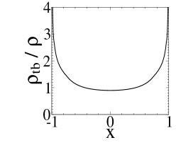
Figure 3: Distribution of tumbling events $\rho_{tb}$ plotted in relation to the distribution of particles $\rho$, corresponding to Fig. (2) (b).

In Fig. (4) we compare (exact) $\rho$ for RTP particles in a harmonic trap for exponential and uniform $p_{t}$, and otherwise for the same set of parameters. The distribution corresponding to a uniform $p_{t}$ is less spread out. This supports our previous claim that the higher agitation of RTP particles near the trap borders prevents those particles to remain in that region. There is some preference for regions with lesser obstructions.

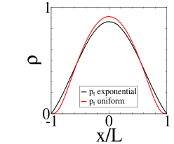
Figure 4: Comparison of particle distributions $\rho(x)$ for exponential and uniform $p_{t}$, for the same set of parameters: $L=\mu K=\tau=v_{0}=1$. $\tau$ is defined as an average value of waiting times $t_{p}$.

In this work, our motivation to examine non-exponential $p_{t}$ came from the study of a simulation. However, the RTP model with non-exponential $p_{t}$ has been considered previously as a better description of a biological system. While exponential $p_{t}$ corresponds to memoryless and Markovian dynamics, any non-exponential $p_{t}$ gives rise to memory effects and non-Markovian dynamics. Recently, non-Markovian RTP model has attracted interest as a potentially more accurate model for describing biological systems, such as bacteria or living cells, where some degree of memory could reasonably be expected to be present Farago and Smith (2024); Detcheverry (2017).

As seen in Fig. (3), non-exponential $p_{t}$ gives rise to a position-dependent frequency of tumbling events. This behavior could be mapped into a position-dependent rate of tumbling. Such a mapping has been carried out for RTP particles in one-dimension in Farago and Smith (2024).

It was determined that the "jump-process" algorithm is limited to an exponential $p_{t}$ — as it represents a memoryless process occurring at a constant rate. For non-exponential cases, we could generalize a "jump-process" algorithm by sampling a single configuration during a single "run" stage at a time, randomly drawn from the interval $t\in[0,t_{p}]$ (rather than at time $t=t_{p}$). To obtain a correct $\rho$, each sampled configuration is multiplied by a statistical weight $t_{p}/\tau$. The advantage of this method over the continuous time method is that there is no need to discretize time.

III.2 probability distribution of jumps $G(x,x^{\prime})$

In this section, we obtain a general expression for the probability distribution of jumps without making assumptions about $p_{t}$. We start with RTP particles in an unconfined environment. Because the "run" stage is deterministic, the distribution during this stage is represented as a propagating delta function, $p(x,x_{0},t,v)=\delta(x-x_{0}-vt)$, where $x_{0}$ is the position at time $t=0$. By assuming $x_{0}=0$ we get $p(x,t,v)=\delta(x-vt)$ which, when averaged over all possible values of $v$, becomes

$$p(x,t)=\int_{-\infty}^{\infty}dv\,p_{v}(v)\delta(x-vt).$$ (5)

The deterministic process lasts for time $t_{p}$ at the end of which the distribution of particles in space (or a distribution of jumps) is $p(x,t_{p})$. Considering all possible $t_{p}$, the probability distribution of jumps becomes

$$G(x)=\int_{0}^{\infty}dt\,p_{t}(t)p(x,t).$$ (6)

Since $G(x)$ in Eq. (6) ignores configurations generated within the interval $t\in[0,t_{p}]$ (that would be sampled during a continuous time simulation), we next try to obtain an analogous quantity to $G(x)$, but that accounts for all configurations in the interval $t\in[0,t_{p}]$.

For a specific value of $t_{p}$, a continuous-time sampling gives rise to a distribution that can be expressed as $\sim\int_{0}^{t_{p}}dt\,p(x,t)$. Account for all possible $t_{p}$ yields

$$g(x)=\frac{1}{\tau}\int_{0}^{\infty}dt_{p}\,p_{t}(t_{p})\int_{0}^{t_{p}}dt\,p(x,t),$$ (7)

where we designate the resulting distribution as $g(x)$ to differentiate it from $G(x)$ in Eq. (6) that only accounts for positions at $t=t_{p}$. The factor $\tau^{-1}$ in front of the integral ensures correct normalization, $\int_{-\infty}^{\infty}dx\,g(x)=1$.

Eq. (7) can be further modified using integration by parts,

$$g(x)=\int_{0}^{\infty}dt\,\frac{S(t)}{\tau}p(x,t),$$ (8)

where

$$S(t)=\int_{t}^{\infty}dt^{\prime}\,p_{t}(t^{\prime})$$ (9)

is the survival function. Since $S(0)=1$ and with the passage of time $S\to 0$, the quantity $S(t)p(x,t)$ represents a distribution that diminishes over time. Details of how Eq. (7) is transformed into Eq. (8) are provided in Appendix (C).

Since $S(t)/\tau$ is normalized, it can be regarded as a probability distribution in time, and we can trace the difference between $g(x)$ in Eq. (8) and $G(x)$ in Eq. (6) to different distributions in time. Comparing Eq. (8) and Eq. (6), indicates that $G(x)\neq g(x)$, thus, the jump-process algorithm, generally, is not a valid sampling method. However, if

$$\frac{S(t)}{\tau}=p_{t}(t),$$

then $G(x)$ and $g(x)$ are identical. This condition is satisfied for a exponential $p_{t}$, $p_{t}(t)=\tau^{-1}e^{-t/\tau}$. For any other functional form of $p_{t}$ we have $S(t)\neq\tau p_{t}(t)$. In those cases, the jump-process algorithm is invalid.

We can obtain similar results for particles in an external potential. As in the previous case, a deterministic distribution during a "run" stage is represented by a propagating delta function. Integrating this distribution over $v$ yields

$$p(x,x_{0},t)=\int_{-v_{0}}^{v_{0}}dv\,p_{v}(v)\delta\left(x-x_{0}-vt-\int_{0}^{t}dt^{\prime}\,\mu F(x(t^{\prime}))\right),$$ (10)

where the term inside the delta function is obtained by integrating the Newtonian equation that governs particle dynamics during the "run" stage,

$$\frac{dx}{dt}=v+\mu F(x),$$ (11)

where $F(x)$ is an external force of some trapping potential. The probability distribution of jumps is obtained by averaging over all possible $t_{p}$,

$$G(x,x_{0})=\int_{0}^{\infty}dt_{p}\,p_{t}(t_{p})p(x,x_{0},t_{p}).$$ (12)

The analogous probability distribution $g(x)$ to that in Eq. (7), that accounts for all the positions during a "run" stage, is given by

$$g(x,x_{0})=\int_{0}^{\infty}dt\,\frac{S(t)}{\tau}p(x,x_{0},t).$$ (13)

Again, $G(x,x_{0})=g(x,x_{0})$ only if $\tau^{-1}S(t)=p_{t}(t)$, which is satisfied only if $p_{t}$ is exponential.

The jump-process sampling method could be used as an alternative simulation method to obtain $\rho$, or as a basis for arriving at an alternative macroscopic description. In this work, we focus on the latter goal.

III.3 distributions $\rho_{tb}(x)$ and $\rho(x)$

Having defined the two operators $G(x,x^{\prime})$ and $g(x,x^{\prime})$, we are in a position to formulate equations for $\rho_{tb}$ and $\rho$. The distribution of tumbling events is obtained from the operator $G(x,x^{\prime})$ using the self-consistent integral equation,

$$\rho_{tb}(x)=\int dx^{\prime}\,\rho_{tb}(x^{\prime})G(x,x^{\prime}),$$ (14)

which expresses the stationarity condition of $\rho_{tb}$ with respect to particle jumps. The distribution $\rho(x)$ is then calculated from $\rho_{tb}$ and $g(x,x^{\prime})$ using another integral equation,

$$\rho(x)=\int dx^{\prime}\,\rho_{tb}(x^{\prime})g(x,x^{\prime}).$$ (15)

The rationale of the second equation is to consider distributions $g(x,x^{\prime})$ (which account for particle positions sampled continuously in time) for all positions $x^{\prime}$, multiplied by the probability of tumbling event $\rho_{tb}(x^{\prime})dx^{\prime}$ corresponding to that point.

Eq. (14) and Eq. (15) provide an alternative framework (to that based on the Fokker-Planck equation) for obtaining $\rho(x)$. The framework affords more flexibility as it is valid for an arbitrary $p_{t}$ (implicit in the operators $G(x,x^{\prime})$ and $g(x,x^{\prime})$). The two equations constitute one of the main results of this paper.

Eq. (15) can be verified by a simulation without a prior calculation of $G(x,x^{\prime})$ and $g(x,x^{\prime})$. We consider the case of particles in a harmonic trap for $d=3$ and uniform $p_{t}$. Such a simulation has two steps. Starting from $x=0$, a particle makes $N$ number of jumps, each representing a single "run" stage. $N$ should be sufficiently large so that a particle position corresponds to the distribution $\rho_{tb}(x)$. During the next "run" stage $N+1$, a simulation collects particle positions continuously in time. The two steps are repeated enough number of times to get good statistics.

In Fig. (5) we plot $\rho(x)$ obtained from the simulation procedure described above for a particle in a harmonic trap $u=Kx^{2}/2$, for a system in $d=3$, and for a uniform $p_{t}$. The distribution is compared with that obtained using a continuous time simulation. The agreement between two distributions confirms the validity of Eq. (15).

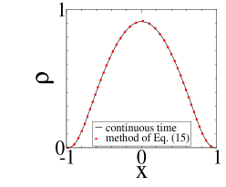
Figure 5: Verification of Eq. (15). The system parameters are the same as those in Fig. (2).

Note that for an exponential $p_{t}$, in which case $\rho(x)=\rho_{tb}(x)$ and $G(x,x^{\prime})=g(x,x^{\prime})$, both Eq. (14) and Eq. (15) lead to a single integral equation for $\rho(x)$,

$$\rho(x)=\int dx^{\prime}\,\rho(x^{\prime})G(x,x^{\prime}).$$ (16)

Thus, for an exponential $p_{t}$, the above equation is sufficient for calculating $\rho$. For non-exponential $p_{t}$ we need to solve both Eq. (14) and Eq. (15).

IV harmonic potential

In the previous section, we have determined general equations for calculating $\rho_{tb}$ and $\rho$. In this section, we consider a concrete example of particles in a harmonic trap $u(x)=Kx^{2}/2$. We consider the standard RTP model corresponding to exponential $p_{t}$. so that $\rho(x)$ is obtained from the self-consistent Eq. (16). To use this equation, we need an analytical expression for the distribution of jumps $G(x,x^{\prime})$.

To obtain $G(x,x^{\prime})$, we note that the motion during the "run" stage is governed by the Newtonian equation

$$\frac{dx}{dt}=-\mu Kx+v,$$ (17)

for which the solution is

$$x(t)=x_{0}e^{-\mu Kt}+\left(1-e^{-\mu Kt}\right)\frac{v}{\mu K}.$$ (18)

Based on this, the probability distribution of jumps can be represented as the propagating delta function averaged over $v$ and $t_{p}$,

$$G(x,x_{0})=\int_{0}^{\infty}dt\,p_{t}\int_{-v_{0}}^{v_{0}}dv\,p_{v}\delta\left(x-x_{0}e^{-\mu Kt}-\frac{v\left(1-e^{-\mu Kt}\right)}{\mu K}\right).$$ (19)

Integrating Eq. (19) over time yields an expression that depends on a relative position of $x$ with respect to $x_{0}$,

$$G_{+}(x,x_{0}<x)=\alpha\int_{x}^{x_{m}}dy\,\frac{p(y)}{y-x_{0}}\left(\frac{y-x}{y-x_{0}}\right)^{\alpha-1}$$

$$G_{-}(x,x_{0}>x)=\alpha\int_{-x_{m}}^{x}dy\,\frac{p(y)}{x_{0}-y}\left(\frac{y-x}{y-x_{0}}\right)^{\alpha-1},$$ (20)

where $\alpha=\frac{1}{\tau\mu K},$ is the dimensionless tumbling rate, $x_{m}=\frac{v_{0}}{\mu K}$ is the maximal distance from the trap center that a particle can reach, and $p(y)$ is related to $p_{v}$ in Eq. (3) and depends on the system dimension,

$$p(y)=\frac{1}{2}\begin{cases}\delta(x_{m}-y)+\delta(x_{m}+y),&\text{for $d=1$},\\ \frac{2}{\pi}\frac{1}{\sqrt{x_{m}^{2}-y^{2}}},&\text{for $d=2$},\\ \frac{1}{x_{m}},&\text{for $d=3$}.\\ \end{cases}$$ (21)

See Appendix (E) for details of how Eq. (20) is derived.

The evaluated form of Eq. (20) depends on a system dimension $d$. Regardless of $d$, however, $G(x,x_{0})$ always vanishes at $x=\pm x_{m}$, unless $x_{0}=\pm x_{m}$. For $d>1$, $G(x,x_{0})$ exhibits a logarithmic singularity at $x=x_{0}$. Such a logarithmic divergence has already been observed for $G(x,x_{0})$ of particles not confined by any potential Frydel (2024b). The presence of a divergence makes exact analysis challenging. Finally, for $d=1$ and $d=3$ the operator $G(x,x_{0})$ is discontinuous at $x=x_{0}$:

$$\Delta G(x)=\begin{cases}\frac{\alpha x}{x_{m}^{2}-x^{2}},&\text{for $d=1$},\\ 0,&\text{for $d=2$},\\ \frac{\alpha}{2x_{m}}\ln\big{(}\frac{x_{m}+x}{x_{m}-x}\big{)},&\text{for $d=3$},\\ \end{cases}$$ (22)

where $\Delta G=\lim_{h\to 0}\big{[}G(x+h,x)-G(x-h,x)\big{]}$ or, alternatively, $\Delta G=\lim_{h\to 0}\big{[}G(x+h,x)-G(x,x+h)\big{]}$.

The transition operator $G(x,x^{\prime})$ contains all the information about a stationary system, such as an external potential and the system dynamics. As we are dealing with a non-equilibrium system, it should be possible to test $G(x,x^{\prime})$ for reversibility. A convenient way to do it is to determine if $G(x,x^{\prime})$ satisfies the Kolmogorov’s criterion, or if $G(x,x^{\prime})$ is reversible over a closed loop of states Meyn et al. (2009). For a loop over three states $x$, $x^{\prime}$, and $x^{\prime\prime}$, the Kolmogorov’s criterion is satisfied if

$$G(x,x^{\prime})G(x^{\prime},x^{\prime\prime})G(x^{\prime\prime},x)=G(x,x^{\prime\prime})G(x^{\prime\prime},x^{\prime})G(x^{\prime},x),$$ (23)

implying that a system is reversible and $\rho(x)$ satisfies the detailed balance condition. If the relation in Eq. (23) is not satisfied, then a system is not reversible.

We may wonder whether the discontinuity in $G(x,x^{\prime})$ at $x=x^{\prime}$ for $d=1$ and $d=3$ in Eq. (22), or its absence for $d=2$, can tell us something of physical significance. More specifically, can it tell us anything about the detailed balance condition Nartallo-Kaluarachchi et al. (2024)

$$\rho(x^{\prime})G(x,x^{\prime})=\rho(x)G(x^{\prime},x).$$

If we take $x^{\prime}=x+h$ such that $h\to 0$ and assume continuous $\rho(x)$, then the detailed balance condition yields $G(x,x+h)=G(x+h,x)$. Due to discontinuities in Eq. (22) for $d=1$ and $d=3$, we know that $G(x+h,x)-G(x,x+h)=\Delta G(x)$, thus, for those cases, the detailed balance condition is violated. It is not clear if the absence of discontinuity for $d=2$ is a sufficient condition for the system to be reversible. We will consider this case in more detail in subsequent sections.

We should emphasize that by discussing $G(x,x^{\prime})$ and its properties, we are no longer describing the original system of RTP particles, but the system onto which the original system was mapped — a jumping particle system with the same stationary distribution as that of the original system.

IV.1 case $d=1$

Because for $d=1$ there are only two possible directions of motion, $v_{swim}=\pm v_{0}$, a stationary distribution $\rho$ can be obtained directly from the Fokker-Planck formulation Tailleur and Cates (2008, 2009); Frydel (2022c), which consists of two coupled differential equations that can be solved exactly — see Eq. (52) in Appendix (A).

We revisit the system in $d=1$ to confirm the validity of the framework based on the transition operator $G(x,x^{\prime})$. For $d=1$, Eq. (20) evaluates to

$$G_{+}(x,x^{\prime})=\frac{\alpha}{2}\frac{1}{x_{m}-x^{\prime}}\left(\frac{x_{m}-x}{x_{m}-x^{\prime}}\right)^{\alpha-1}$$

$$G_{-}(x,x^{\prime})=\frac{\alpha}{2}\frac{1}{x_{m}+x^{\prime}}\left(\frac{x_{m}+x}{x_{m}+x^{\prime}}\right)^{\alpha-1}.$$ (24)

As we have already determined, due to the presence of discontinuity of $G(x,x^{\prime})$ at $x=x^{\prime}$, the system does not satisfy the detailed balance condition nor Kolmogorov’s criterion in Eq. (23). Thus, both the original system of RTP particles and the auxiliary system are out-of-equilibrium.

To obtain $\rho(x)$ from $G(x,x^{\prime})$, we use Eq. (16). Due to discontinuity of $G(x,x^{\prime})$ at $x=x^{\prime}$, this equation is more conveniently written as

$$\rho(x)=\int_{-x_{m}}^{x}dx^{\prime}\,\rho(x^{\prime})G_{+}(x,x^{\prime})+\int_{x}^{x_{m}}dx^{\prime}\,\rho(x^{\prime})G_{-}(x,x^{\prime}).$$ (25)

By differentiating the above equation with respect to $x$, we get the following differential equation

$$(x_{m}^{2}-x^{2})\rho^{\prime}=x\rho-(\alpha-1)x_{m}q,$$ (26)

where

$$q=\int_{-x_{m}}^{x}dx^{\prime}\,\rho(x^{\prime})G_{+}(x,x^{\prime})-\int_{x}^{x_{m}}dx^{\prime}\,\rho(x^{\prime})G_{-}(x,x^{\prime}).$$ (27)

Note that the sole difference between $q$ and $\rho$ in Eq. (25) is the sign before the second term. Taking the derivative of $q$, leads to another differential equation,

$$(x_{m}^{2}-x^{2})q^{\prime}=x_{m}\rho-(\alpha-1)xq.$$ (28)

Eq. (26) and Eq. (28) can be combined to yield a second-order differential equation

$$0=(\alpha-2)\rho+(\alpha-4)x\rho^{\prime}+(x_{m}^{2}-x^{2})\rho^{\prime\prime},$$

which can be reduced to a first-order differential equation given by

$$0=(\alpha-2)x\rho+(x_{m}^{2}-x^{2})\rho^{\prime},$$ (29)

for which the solution is

$$\rho\propto(x_{m}^{2}-x^{2})^{\frac{\alpha}{2}-1}.$$ (30)

Details of the derivation can be found in Appendix (F).

Both Eq. (29) and the solution in Eq. (30) agree with the known exact results obtained directly from the Fokker-Planck equation. This re-derivation confirms the validity of the alternative formulation of the same problem.

IV.2 case $d=2$

For the case $d=2$, the formula in Eq. (20) evaluates to

$$G(x,x^{\prime}) = \frac{\Gamma(\alpha+1)}{2^{\alpha}\sqrt{\pi}\Gamma(\alpha+1/2)}\sqrt{\frac{1}{x_{m}^{2}-x^{\prime 2}}}\left(\frac{x_{m}^{2}-x^{2}}{x_{m}^{2}-x^{\prime 2}}\right)^{\frac{\alpha}{2}-\frac{1}{2}}$$ (31)

$$w^{\alpha/2}\,\,\,_{2}F_{1}\left(\frac{\alpha}{2},\frac{\alpha}{2}+\frac{1}{2},\alpha+\frac{1}{2},w\right),$$

where ${}_{2}F_{1}$ is the hypergeometric function. To simplify the nomenclature, we introduce a dimensionless parameter

$$w=\left[1+\frac{(x-x^{\prime})^{2}x_{m}^{2}}{(x_{m}^{2}-x^{2})(x_{m}^{2}-x^{\prime 2})}\right]^{-1}.$$

In Sec. (IV) we determined that the absence of discontinuity in $G(x,x^{\prime})$ did not permit us to determine if $G(x,x^{\prime})$ violates the detailed balance condition. Using the Kolmogorov’s test in Eq. (23) we find that $G(x,x^{\prime})$ in Eq. (31) is reversible over any closed loop, which implies that $\rho(x)$ satisfies the detailed balance condition,

$$\rho(x)G(x^{\prime},x)=\rho(x^{\prime})G(x,x^{\prime}).$$ (32)

The equation above can be used to define $\rho(x)$ as $\rho(x)=\rho(x^{\prime}){G(x,x^{\prime})}/{G(x^{\prime},x)}.$ For convenience we select $x^{\prime}=0$, leading to $\rho(x)=\rho(0){G(x,0)}/{G(0,x)}$. Since $\rho(0)$ functions as a normalization constant, which could be determined at any point, we ignore it. By choosing any other $x^{\prime}$, we could represent the unnormalized distribution as

$$\rho(x)\propto\frac{G(x,x^{\prime})}{G(x^{\prime},x)}.$$ (33)

Using the formula in Eq. (31), the stationary distribution based on the above equation becomes

$$\rho(x)\propto\left(x_{m}^{2}-x^{2}\right)^{\alpha-\frac{1}{2}},$$ (34)

whose functional form is the same as that for $\rho$ in Eq. (30) — despite the fact that $G(x,x^{\prime})$ for each case is significantly different. Not only this, but in one case it is irreversible and in another reversible.

Since the original system of RTP particles is out-of-equilibrium, reversibility is a property of the auxiliary system governed by the jump-process. The significance of the reversibility is that it simplifies the mathematics of the problem, leading to exact and simple results.

IV.3 case $d=3$

The case $d=3$ is most challenging of all dimensions. Its complexity is manifest in algebraic expressions of the moments $\langle x^{2n}\rangle$ of $\rho(x)$, which can be obtained by converting the Fokker-Planck equation into the recurrence relation Frydel (2022c, 2023a),

$$\langle z^{2n}\rangle=\frac{\alpha}{2n}\sum_{k=0}^{n-1}\frac{\langle z^{2k}\rangle}{2n-2k+1}\frac{(2k+1)_{\alpha-1}}{(2n+1)_{\alpha-1}},$$ (35)

where $(a)_{n}=a(a-1)\dots(a-n+1)$ is the falling factorial, and $z=x/x_{m}$. Because the recurrence relation cannot be solved; the moments are generated sequentially. As in principle, we can generate an algebraic expression for all the moments, we should have all the information about $\rho(x)$. The difficult part is how to extract $\rho(x)$ from $\langle x^{2n}\rangle$. There is no standard technique for converting moments into a distribution. It is, therefore, interesting to see what the framework based on $G(x,x^{\prime})$ has to say about the case $d=3$.

For the case $d=3$, Eq. (20) evaluates to

$$G(x,x^{\prime})=\frac{1}{2}\frac{1}{x_{m}}w^{\alpha}\,\,\,_{2}F_{1}\big{(}\alpha,\alpha,1+\alpha,-w\big{)},$$ (36)

where ${}_{2}F_{1}$ is the hypergeometric function and

$$w=\frac{x_{m}}{|x-x^{\prime}|}-\frac{x}{x-x^{\prime}}.$$ (37)

We have already determined in Sec. (IV), $G(x,x^{\prime})$ is not reversible and the corresponding $\rho(x)$ does not obey the detailed balance condition due to the presence of discontinuity in $G(x,x^{\prime})$.

We proceed in a manner similar to that for the case $d=1$ and differentiate Eq. (25) with respect to $x$. This yields an integro-differential equation

$$0 = \alpha\rho\ln\left(\frac{x_{m}+x}{x_{m}-x}\right)+2x_{m}\rho^{\prime}$$ (38)

$$+ \alpha\int_{-x_{m}}^{x}dx^{\prime}\,\frac{\rho(x^{\prime})}{x-x^{\prime}}\left(\frac{x_{m}-x}{x_{m}-x^{\prime}}\right)^{\alpha-1}$$

$$+ \alpha\int_{x}^{x_{m}}dx^{\prime}\,\frac{\rho(x^{\prime})}{x-x^{\prime}}\left(\frac{x_{m}+x}{x_{m}+x^{\prime}}\right)^{\alpha-1},$$

not exactly a simple result, but at least without hypergeometric functions.

To make expressions more transparent to interpretation, we consider a specific case $\alpha=1$. The integro-differential equation in this case can be written as

$$j=-v_{0}\left[\frac{\rho}{2}\ln\left(\frac{x_{m}+x}{x_{m}-x}\right)+\frac{1}{2}\int_{-x_{m}}^{x_{m}}dx^{\prime}\,\frac{\rho(x^{\prime})}{x-x^{\prime}}\right]-D_{eff}\rho^{\prime},$$ (39)

where $j$ represents the flux such that for a stationary state $j=0$ it recovers Eq. (38) for $\alpha=1$. The last term in the equation represents flux due to diffusion, where $D_{eff}=v_{0}^{2}\tau$ is the effective diffusion constant. The two terms in square brackets represent velocity due to the effective forces of the system. The first term can be linked to an effective external potential. The second term involving an integral almost looks like a mean-field contribution of (effective) particle interactions. However, to look like a mean-field term, it would need to be proportional to $\rho(x)$, and it is not. Also, strictly speaking, the mean-field-like term would imply that $G(x,x^{\prime})$ is reversible, but we already know it is not. What is certain is that the integral term is responsible for non-reversibility of the system.

IV.3.1 jump-process simulation

The alternative formulation offers some insights as to why an expression for $\rho(x)$ in $d=3$ is so difficult to get. As for the cases $d=1$ and $d=3$, $\rho$ satisfies a first-order differential equation, for $d=3$ it satisfies a complicated integro-differential equation, which requires some sort of numerical assistance in order to be solved.

One numerical approach is to use the jump-process algorithm in which a particle, rather than moving continuously in time, makes sequential jumps. Consecutive particle positions, using Eq. (18), are given by

$$x_{n+1}=x_{n}e^{-\mu Kt_{p}}+\left(1-e^{-\mu Kt_{p}}\right)\frac{v}{\mu K}.$$ (40)

A new position depends on two random variables, $t_{p}$ which is drawn from an exponential distribution, and $v$ drawn from the uniform distribution $p_{v}$ on the interval $v\in[-v_{0},v_{0}]$. The advantage of this algorithm over the continuous time algorithm is that there is no need to introduce a discrete time interval.

IV.3.2 numerical iteration

Another numerical method involves solving Eq. (16) numerically via iterative procedure,

$$\rho_{n+1}(x)=\int_{-x_{m}}^{x_{m}}dx^{\prime}\,\rho_{n}(x^{\prime})G(x,x^{\prime}),$$ (41)

for some initial distribution $\rho_{0}$ that we choose to be uniform, $\rho_{0}=1/2x_{m}$. Since $\rho$ for $\alpha=0$ is uniform, we expect that the number of iterations necessary for $\rho_{n}$ to converge to $\rho$ increases with increasing $\alpha$.

In Fig. (6) we plot the iterated distribution $\rho_{n}$ (for $\alpha=1$) for $n=1,2,5$. The distribution $\rho_{5}$ is almost indistinguishable from the exact $\rho$, indicating fast convergence.

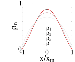
Figure 6: $\rho_{n}$ for $n=1,2,5$ obtained from numerical iterations in to Eq. (41) for the initial distribution $\rho_{0}=1/2x_{m}$ and $\alpha=1$.

In Fig. (7) we plot a number of different distributions for different values of $\alpha$, calculated numerically from Eq. (41) and compare it to $\rho$ obtained from a continuous time simulation. A match between the two distributions confirms efficiency of the iterative procedure.

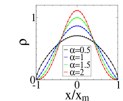
Figure 7: $\rho$ calculated from the numerical procedure in Eq. (41) for different values of $\alpha$. The circular points represent the data points generated from a continuous time simulation.

IV.3.3 analytical approach: case $\alpha=1$

In this section, we propose a semi-analytic approach based on a truncated series

$$\rho_{M}(z)\propto 1+\sum_{n=1}^{M}a_{n}z^{2n},$$ (42)

where $z=x/x_{m}$.

To determine the coefficients $a_{n}$, we insert $\rho_{M}$ into Eq. (38). The terms proportional to a given power of $z$ can be segregated into different groups. Since each group of terms should vanish if Eq. (38) is to be satisfied, this leads to $M$ independent equations which can be represented as

$$\sum_{m=1}^{N}A_{nm}a_{m}=b_{n}$$ (43)

where $b_{n}=A_{n,0}$. The coefficients $A_{nm}$ can be represented by a square $M\times M$ matrix and the coefficients $b_{n}$ by a vector of size $M$. For $\alpha=1$, the elements of the vector $b$ and the matrix $A$ have the following form

$$b_{n}=-\frac{2}{2n-1},$$ (44)

and

$$A_{mn}=\frac{u(m-n)}{2m-2n-1}+\frac{1}{2m-2n-1}+\frac{2m}{\alpha}\delta_{mn},$$ (45)

where

$$u(n)=\begin{cases}1,&\text{if $n>0$}.\\ 0,&\text{if $n\leq 0$}.\end{cases}$$ (46)

is the unit step function.

By representing Eq. (43) as $Aa=b$, the coefficients $a_{n}$ can be obtained from the relation $a=bA^{-1},$ where $A^{-1}$ is an inverse of $A$. The stationary distribution is then obtained by normalizing the truncated sequence in Eq. (42) as

$$\rho_{M}(z)=\frac{1}{2}\frac{1+\sum_{n=1}^{M}a_{n}z^{2n}}{1+\sum_{n=1}^{M}a_{n}/(2n+1)}.$$ (47)

Appendix (G) shows a simple Mathematica code for generating $\rho_{M}(z)$ for any arbitrary number of terms $M$. Already $M=10$ yield a highly accurate distribution.

V uniform $p_{t}$

In this section, we consider RTP particles in a harmonic trap for non-exponential $p_{t}$ with focus on a uniform $p_{t}$. The main purpose is to get insights about reasons why $G(x,x^{\prime})$ in $d=2$ is reversible and if that reversibility is broken by a non-exponential $p_{t}$.

It turns out that one can obtain an exact expression for the discontinuity, defined as $\Delta G=\lim_{h\to 0}\big{[}G(x+h,x)-G(x-h,x)\big{]}$, for a general $p_{t}$ and given below for different $d$

$$\Delta G(x)=\begin{cases}\frac{p_{t}(0)}{\mu K}\frac{x}{x_{m}^{2}-x^{2}},&\text{for $d=1$},\\ 0,&\text{for $d=2$},\\ \frac{p_{t}(0)}{\mu K}\frac{1}{2x_{m}}\ln\big{(}\frac{x_{m}+x}{x_{m}-x}\big{)},&\text{for $d=3$}.\\ \end{cases}$$ (48)

where for a uniform $p_{t}$, defined as $p_{t}=(2\tau)^{-1}\Theta(2\tau-t)$, we have $p_{t}(0)=1/2\tau$. According to the above result, a discontinuity in $G(x,x^{\prime})$ is absent for the case $d=2$, independently of the functional form of $p_{t}$. Its absence seems to be caused by the specific form of $p_{v}$ defined in Eq. (3).

The next question is, is the absence of discontinuity enough to make $G(x,x^{\prime})$ reversible, or do we also need a memoryless (exponential) distribution $p_{t}$.

We can answer this question for a specific case corresponding to a uniform $p_{t}$. If $\rho_{tb}$, as defined in Eq. (14), obeyed the detailed balance condition, it could be represented as

$$\rho_{tb}(x)\propto\frac{G(x,0)}{G(0,x)},$$ (49)

see Eq. (33) for a similar expression. For a uniform $p_{t}$, $G(x,0)$ vanishes outside the interval $1-e^{-2/\alpha}<x/x_{m}<1-e^{-2/\alpha}.$ We calculate the limits of the interval using Eq. (18) for $t=2\tau$, which corresponds to the maximal $t_{p}$ of the uniform $p_{t}$. However, since $\rho_{tb}(x)$ is defined on $-1<x/x_{m}<1$, Eq. (49) could not be satisfied.

Based on this, we conclude that for a uniform $p_{t}$, the operator $G(x,x^{\prime})$ for the case $d=2$ is not reversible. This means, in addition to the absence of a discontinuity, reversibility requires the second condition that the distribution $p_{t}$ be memoryless.

VI Conclusion

By reinterpreting RTP motion as jump-process, we arrive at an alternative formulation of the stationary system. Transformation from one microscopic process to another is implemented by neglecting configurations generated during the "run" stage of the run-and-tumble motion. Such sampling, however, amounts to calculating the distribution of "tumbling" events. If the distribution of waiting times $t_{p}$ is memoryless (or exponential), this distribution is the same as the distribution of particles, leading to a self-consistent formulation in Eq. (16). For any other $p_{t}$, the formulation requires two integral equations, Eq. (14) and Eq. (15).

For $d=1$, the formalism based on Eq. (16) reproduces known exact results, confirming the accuracy of the formalism. The case $d=2$ is more interesting. The transition operator $G(x,x^{\prime})$ in this case satisfies Kolmogorov’s criterion, implying that $G(x,x^{\prime})$ is reversible over any closed loop of states and that $\rho$ satisfies the detailed balance condition. A stationary distribution in this case can be obtained directly from $G(x,x^{\prime})$ using Eq. (33), which significantly simplifies the problem. The resulting $\rho$ has the same functional form as that for the case $d=1$.

It can be determined that $G(x,x^{\prime})$ for $d=2$ owes its property of reversibility to two conditions, the absence of discontinuity in $G(x,x^{\prime})$, and the memoryless distribution of waiting times $p_{t}$.

The case $d=3$ is the most complex. The resulting $G(x,x^{\prime})$ is non-reversible and $\rho$ can only be obtained from the integral equation in Eq. (16). This equation offers some insights about why $\rho$ evades analytical tractability, but otherwise, it needs to be solved numerically. which provides an alternative route to simulations for obtaining $\rho$.

VII DATA AVAILABILITY

The data that support the findings of this study are available from the corresponding author upon reasonable request.

Appendix A Fokker-Planck equation for a general dimension

In this section, we generalize the Fokker-Planck equation for RTP particles in confinement given in Eq. (1) specifically for dimension $d=2$. A general form of this equation, for a dimension $d>1$, could be written as

$$\frac{\partial n}{\partial t} = -\mbox{\boldmath$\nabla$}\cdot\left[\left({\bf F}+v_{0}{\bf u}\right)n\right]-\frac{1}{\tau}\left(n-\frac{1}{\int d\Omega}\int d\Omega\,n\right)$$ (50)

where $\Omega$ is a solid angle. The integral considers all orientations of a swimming velocity whose magnitude is constant $|{\bf v}_{swim}|=v_{0}$. For dimension $d=3$, where $d\Omega=d\theta d\phi\sin\phi$, the Fokker-Planck equation becomes

$$\frac{\partial n}{\partial t} = -\mbox{\boldmath$\nabla$}\cdot\left[\left({\bf F}+v_{0}{\bf u}\right)n\right]$$ (51)

$$- \frac{1}{\tau}\left(n-\frac{1}{4\pi}\int_{0}^{2\pi}d\theta\int_{0}^{\pi}d\phi\,\sin\phi n({\bf r},\theta,\phi,t)\right)$$

where $n\equiv n({\bf r},\theta,\phi,t)$.

For the system in $d=1$, there are only two possible swimming orientations. In this case, the distribution of particles with forward and backward direction of motion are represented as $n_{+}$ and $n_{-}$, respectively, and the Fokker-Planck equation is represented as two coupled differential equations:

$$\frac{\partial n_{+}}{\partial t}=-\mbox{\boldmath$\nabla$}\cdot\left[\left({F}+v_{0}\right)n_{+}\right]-\frac{1}{\tau}\left(n_{+}-n_{-}\right)$$

$$\frac{\partial n_{-}}{\partial t}=-\mbox{\boldmath$\nabla$}\cdot\left[\left({F}-v_{0}\right)n_{+}\right]-\frac{1}{\tau}\left(n_{-}-n_{+}\right).$$ (52)

Appendix B Derivation of the probability distributions $p_{v}$

To obtain the probability distribution for the projection of the swimming velocity along the $x$-axis, $v=v_{0}\cos\theta$, we start by considering the fact that in the polar coordinates, the swimming velocity is uniformly distributed over the angle $\theta$. Such a uniform distribution on the interval $\theta\in[0,2\pi]$ is given by $p_{\theta}=1/(2\pi)$. The projection of the swimming velocity along the $x$-axis will be distributed on the interval $v\in[-v_{0},v_{0}]$. To obtain this distribution, we start with the integral $\frac{1}{2\pi}\int_{0}^{2\pi}d\theta\,p_{\theta}(\theta)$ and then apply a change of a variable,

$$v=v_{0}\cos\theta,~~~dv=-v_{0}\sin\theta d\theta=-d\theta\sqrt{v_{0}^{2}-v^{2}}.$$ (53)

This yields

$$\frac{1}{2\pi}\int_{0}^{2\pi}d\theta=-\frac{1}{\pi}\int_{-v_{0}}^{v_{0}}dv\,\frac{d\theta}{dv}=\frac{1}{\pi}\int_{-v_{0}}^{v_{0}}dv\,\frac{1}{\sqrt{v_{0}^{2}-v^{2}}}.$$ (54)

From the final expression we conclude that the distribution in $v$ is

$$p_{v}=\frac{1}{\pi}\frac{1}{\sqrt{v_{0}^{2}-v^{2}}}.$$ (55)

This expression appears in Eq. (3) and corresponds to the case $d=2$.

In the case $d=3$ we work with spherical coordinates. In this case, the orientation of any vector is parametrized by two parameters, $\theta$ and $\phi$. The orientation of a swimming orientation is uniformly distributed over a solid angle $\Omega(\theta,\phi)$. And because in spherical coordinates the integral over a solid angle is $\int_{0}^{2\pi}d\phi\int_{0}^{\pi}d\theta\,\sin\theta$, we start from this integral and then transform it into the integral over $v$ using a change of a variable in Eq. (53). This yields

$$\frac{1}{4\pi}\int_{0}^{2\pi}d\phi\int_{0}^{\pi}d\theta\,\sin\theta=-\frac{1}{2}\int_{-v_{0}}^{v_{0}}dv\,\frac{d\theta}{dv}\sin\theta=\frac{1}{2}\frac{1}{v_{0}}\int_{-v_{0}}^{v_{0}}dv.$$ (56)

From the final expression we conclude that the distribution in $v$ is uniform on the interval $v\in[-v_{0},v_{0}]$:

$$p_{v}=\frac{1}{2}\frac{1}{v_{0}}.$$ (57)

This expression appears in Eq. (3).

Appendix C Derivation of Eq. (8)

In the main body of this work, the expression in Eq. (7) is converted to Eq. (8). In this section we provide more details of this transformation. For clarity we repeat Eq. (7) below

$$g(x)=\frac{1}{\tau}\int_{0}^{\infty}dt_{p}\,p_{t}(t_{p})\left[\int_{0}^{t_{p}}dt\,p(x,t)\right].$$ (58)

Using integration by parts, we express the above integral as

$$g(x) = -\frac{1}{\tau}\int_{0}^{\infty}dt_{p}\,\frac{d}{dt_{p}}\left[\int_{0}^{t_{p}}dt\,p(x,t)\right]\int_{0}^{t_{p}}dt\,p_{t}(t)$$ (59)

$$+ \frac{1}{\tau}\left[\left(\int_{0}^{t_{p}}dt\,p_{t}(t)\right)\left(\int_{0}^{t_{p}}dt\,p(x,t)\right)\right]_{0}^{\infty}$$

After some evaluation, the above expression reduces to

$$g(x)=-\frac{1}{\tau}\int_{0}^{\infty}dt_{p}\,p(x,t_{p})\int_{0}^{t_{p}}dt\,p_{t}(t)+\frac{1}{\tau}\int_{0}^{\infty}dt\,p(x,t).$$ (60)

Since $\int_{0}^{t_{p}}dt\,p_{t}(t)=1$, we can write

$$\int_{0}^{t_{p}}dt\,p_{t}(t)=1-\int_{t_{p}}^{\infty}dt\,p_{t}(t).$$

Inserting the above identity into Eq. (60) leads to

$$g(x)=\frac{1}{\tau}\int_{0}^{\infty}dt_{p}\,p(x,t_{p})\int_{t_{p}}^{\infty}dt\,p_{t}(t).$$ (61)

Finally, given the definition of the survival function,

$$S(t)=\int_{t}^{\infty}dt^{\prime}\,p_{t}(t^{\prime}),$$ (62)

Eq. (61) recovers the expression in Eq. (8), given below for calrity

$$g(x)=\frac{1}{\tau}\int_{0}^{\infty}dt\,S(t)p(x,t).$$ (63)

Appendix D Details on the derivation of Eq. (20)

In this section we provide details of how to transform Eq. (19), given below for clarity,

$$G=\int_{0}^{2\tau}dt\,\int_{-v_{0}}^{v_{0}}dv\,p_{v}\delta\left(x-x_{0}e^{-\mu Kt}-\frac{v\left(1-e^{-\mu Kt}\right)}{\mu K}\right),$$ (64)

into Eq. (20). We start by rewriting the above equation as

$$G=\frac{1}{2\tau}\int_{-v_{0}}^{v_{0}}dv\,p_{v}\int_{0}^{2\tau}dt\,\delta\left(x-\frac{v}{\mu K}+\left(\frac{v}{\mu K}-x_{0}\right)e^{-\mu Kt}\right),$$ (65)

where we assume a uniform $p_{t}$, and then change the sequence of integrations. In the next step, we use a change of a variable

$$s=e^{-\mu Kt},~~~~~ds=-\mu Ksdt,$$

which also permits us to write $e^{-t/\tau}=s^{\alpha}$, where $\alpha=(\tau\mu K)^{-1}$. Changing the variables in Eq. (72) leads to

$$G=\frac{\alpha}{2}\int_{-v_{0}}^{v_{0}}\frac{dv}{\mu K}\,\frac{\mu Kp_{v}}{|x_{0}-\frac{v}{\mu K}|}\int_{e^{-2\mu K\tau}}^{1}ds\,s^{-1}\delta\left(s-\frac{x-\frac{v}{\mu K}}{x_{0}-\frac{v}{\mu K}}\right),$$ (66)

where we used $\int_{-\infty}^{\infty}dx\,\delta(xa)=\frac{1}{|a|}\int_{-\infty}^{\infty}dx\,\delta(x)$. We next simplify the nomenclature and define $y=\frac{v}{\mu K}.$ This allows us to write the above equation as

$$G=\frac{\alpha}{2}\int_{-x_{m}}^{x_{m}}dy\,\frac{p(y)}{|y-x_{0}|}\int_{e^{-2/\alpha}}^{1}ds\,s^{-1}\delta\left(s-\frac{y-x}{y-x_{0}}\right),$$ (67)

and where $p(y)$ is related to $p_{v}(v)$ and is defined in Eq. (21). We are now in the position to evaluate the integral over $s$. A simple minded integration yields

$$G=\frac{\alpha}{2}\int_{-x_{m}}^{x_{m}}dy\,\frac{p(y)}{|y-x_{0}|}\left(\frac{y-x}{y-x_{0}}\right)^{-1}\Theta\left[\left(A-e^{-2/\alpha}\right)\left(1-A\right)\right]$$ (68)

where $x_{m}=\frac{v_{0}}{\mu K}.$

$$G=\frac{\alpha}{4}\frac{1}{|x_{m}-x_{0}|}\left(\frac{x_{m}-x}{x_{m}-x_{0}}\right)^{-1}\Theta\left[\left(\frac{x_{m}-x}{x_{m}-x_{0}}-e^{-2/\alpha}\right)\left(\frac{x-x_{0}}{x_{m}-x_{0}}\right)\right]$$ (69)

$$G=\frac{\alpha}{4}\left(1-x\right)^{-1}\Theta\left[\left(1-e^{-2/\alpha}-x\right)\left(x\right)\right]$$ (70)

However, the integral over $s$ involves limits. We can incorporates these limits indirectly by observing that to avoid imaginary numbers due to the term $(\frac{y-x}{y-x_{0}})^{-1}$ we need to make sure that either $y>x$ and $y>x_{0}$, which, when implemented yields

$$G_{+}(x,x_{0})=\frac{\alpha}{2}\int_{x}^{x_{m}}dy\,\frac{p(y)}{y-x_{0}}\left(\frac{y-x}{y-x_{0}}\right)^{-1},$$

or $y<x$ and $y<x_{0}$, which, when implemented yields

$$G_{-}(x,x_{0})=\frac{\alpha}{2}\int_{-x_{m}}^{x}dy\,\frac{p(y)}{x_{0}-y}\left(\frac{y-x}{y-x_{0}}\right)^{-1}.$$

Finally, we note that in order for both equations to be positive, $G_{+}(x,x_{0}<x)$ and $G_{-}(x,x_{0}>x)$. We now recover the expressions in Eq. (20).

Appendix E Details on the derivation of Eq. (20)

In this section we provide details of how to transform Eq. (19), given below for clarity,

$$G=\int_{0}^{\infty}dt\,p_{t}\int_{-v_{0}}^{v_{0}}dv\,p_{v}\delta\left(x-x_{0}e^{-\mu Kt}-\frac{v\left(1-e^{-\mu Kt}\right)}{\mu K}\right),$$ (71)

into Eq. (20). We start by rewriting the above equation as

$$G=\frac{1}{\tau}\int_{-v_{0}}^{v_{0}}dv\,p_{v}\int_{0}^{\infty}dt\,e^{-t/\tau}\delta\left(x-\frac{v}{\mu K}+\left(\frac{v}{\mu K}-x_{0}\right)e^{-\mu Kt}\right),$$ (72)

where we assume an exponential distribution $p_{t}=\tau^{-1}e^{-t/\tau}$, and then change the sequence of integrations. In the next step, we use a change of a variable

$$s=e^{-\mu Kt},~~~~~ds=-\mu Ksdt,$$

which also permits us to write $e^{-t/\tau}=s^{\alpha}$, where $\alpha=(\tau\mu K)^{-1}$. Changing the variables in Eq. (72) leads to

$$G=\alpha\int_{-v_{0}}^{v_{0}}\frac{dv}{\mu K}\,\frac{\mu Kp_{v}}{|x_{0}-\frac{v}{\mu K}|}\int_{0}^{1}ds\,s^{\alpha-1}\delta\left(s-\frac{x-\frac{v}{\mu K}}{x_{0}-\frac{v}{\mu K}}\right),$$ (73)

where we used $\int_{-\infty}^{\infty}dx\,\delta(xa)=\frac{1}{|a|}\int_{-\infty}^{\infty}dx\,\delta(x)$. We next simplify the nomenclature and define $y=\frac{v}{\mu K}.$ This allows us to write the above equation as

$$G=\alpha\int_{-x_{m}}^{x_{m}}dy\,\frac{p(y)}{|x_{0}-y|}\int_{0}^{1}ds\,s^{\alpha-1}\delta\left(s-\frac{x-y}{x_{0}-y}\right),$$ (74)

and where $p(y)$ is related to $p_{v}(v)$ and is defined in Eq. (21). We are now in the position to evaluate the integral over $s$. A simple minded integration yields

$$G=\alpha\int_{-x_{m}}^{x_{m}}dy\,\frac{p(y)}{|x_{0}-y|}\left(\frac{y-x}{y-x_{0}}\right)^{\alpha-1},$$ (75)

where $x_{m}=\frac{v_{0}}{\mu K}.$ However, the integral over $s$ involves limits. We can incorporates these limits indirectly by observing that to avoid imaginary numbers due to the term $(\frac{y-x}{y-x_{0}})^{\alpha-1}$ we need to make sure that either $y>x$ and $y>x_{0}$, which, when implemented yields

$$G_{+}(x,x_{0})=\alpha\int_{x}^{x_{m}}dy\,\frac{p(y)}{y-x_{0}}\left(\frac{y-x}{y-x_{0}}\right)^{\alpha-1},$$

or $y<x$ and $y<x_{0}$, which, when implemented yields

$$G_{-}(x,x_{0})=\alpha\int_{-x_{m}}^{x}dy\,\frac{p(y)}{x_{0}-y}\left(\frac{y-x}{y-x_{0}}\right)^{\alpha-1}.$$

Finally, we note that in order for both equations to be positive, $G_{+}(x,x_{0}<x)$ and $G_{-}(x,x_{0}>x)$. We now recover the expressions in Eq. (20).

Appendix F Derivation of $\rho$ for the case $d=1$

In this section we show how the two differential equations, Eq. (26) and Eq. (28), shown again below for clarity,

$$(x_{m}^{2}-x^{2})\rho^{\prime}=x\rho-(\alpha-1)x_{m}q,$$

$$(x_{m}^{2}-x^{2})q^{\prime}=x_{m}\rho-(\alpha-1)xq,$$ (76)

are combined into a single differential equation. We start by using the first equation above to obtain an expression for $q$, by rearrangement, and then for $q^{\prime}$, by taking derivative of that expression. This leads to

$$(\alpha-1)x_{m}q=x\rho-(x_{m}^{2}-x^{2})\rho^{\prime}$$

$$(\alpha-1)x_{m}q^{\prime}=\rho+3x\rho^{\prime}-(x_{m}^{2}-x^{2})\rho^{\prime\prime}.$$ (77)

The above equations are then inserted into the second equation in Eq. (76). We first substitute for $q$, which after some algebraic manipulation yields

$$(x_{m}^{2}-x^{2})x_{m}q^{\prime}=(x_{m}^{2}-x^{2})\rho+(x_{m}^{2}-x^{2})x\rho^{\prime},$$

and then for $q^{\prime}$, which after manipulation yields

$$0=(\alpha-2)\rho+(\alpha-4)x\rho^{\prime}+(x_{m}^{2}-x^{2})\rho^{\prime\prime}.$$ (78)

Finally, we note that the above second-order differential equation can be written as

$$0=(\alpha-2)[x\rho]^{\prime}-[x^{2}\rho^{\prime}]^{\prime}+x_{m}^{2}\rho^{\prime\prime}.$$

which after integration becomes

$$\text{const}=(\alpha-2)x\rho-x^{2}\rho^{\prime}+x_{m}^{2}\rho^{\prime},$$ (79)

where we still need to determine the constant parameter on the left-hand-side. To do this, we choose the most convenient point, $x=0$. This eliminates the first two terms on the right-hand-side, yielding $\text{const}=x_{m}^{2}\rho^{\prime}(0)$. We also know that $\rho(x)$ is an even function, due to symmetry of the harmonic potential. This means that $\rho^{\prime}(0)=0$, thus, $\text{const}=0$, and Eq. (79) becomes

$$0=(\alpha-2)x\rho+(x_{m}^{2}-x^{2})\rho^{\prime},$$ (80)

which recovers the first-order differential equation in Eq. (29).

Appendix G Mathematica implementation of analytical approach in Sec. (IV.3.3)

In this section we show a simple Mathematica code for generating a truncated series $\rho_{M}(z)\propto 1+\sum_{n=1}^{M}a_{n}z^{2n}$, for $\alpha=1$, as explained in Sec. (IV.3.3).

$M=10;$

$\text{A}=\text{Table}\left[\frac{\text{UnitStep}[n-m-1]}{2m-2n-1}+\frac{1}{2m-2n-1}+2m\text{KroneckerDelta}[n-m],\{m,M\},\{n,M\}\right];$

$\text{b}=\text{Table}[-\frac{2}{2n-1},\{n,M\}];$

$\text{IA}=\text{Inverse}[\text{A}];$

$a=\text{IA}.\text{b};$

$\text{norm}=2+\sum_{n=1}^{M}\frac{2a[[n]]}{1+2n}$

$\text{rho[z\_]}:=\left(1+\sum_{n=1}^{M}a[[n]]z^{2n}\right)/\text{norm}$

References

- Tailleur and Cates (2008) J. Tailleur and M. E. Cates, Phys. Rev. Lett. 100, 218103 (2008).
- Tailleur and Cates (2009) J. Tailleur and M. E. Cates, Europhysics Letters 86, 60002 (2009).
- Grognot and Taute (2021) M. Grognot and K. M. Taute, Current Opinion in Microbiology 61, 73 (2021).
- Malakar et al. (2018) K. Malakar, V. Jemseena, A. Kundu, K. V. Kumar, S. Sabhapandit, S. N. Majumdar, S. Redner, and A. Dhar, Journal of Statistical Mechanics: Theory and Experiment 2018, 043215 (2018).
- Razin (2020) N. Razin, Phys. Rev. E 102, 030103 (2020).
- Berg (1983) H. C. Berg, Random Walks in Biology (Princeton University Press, Princeton, NJ, 1983).
- Schnitzer (1993) M. J. Schnitzer, Phys. Rev. E 48, 2553 (1993).
- Romanczuk et al. (2012) P. Romanczuk, M. Bär, W. Ebeling, B. Lindner, and L. Schimansky-Geier, The European Physical Journal Special Topics 202, 1 (2012).
- Fily and Marchetti (2012) Y. Fily and M. C. Marchetti, Phys. Rev. Lett. 108, 235702 (2012).
- Marchetti et al. (2013) M. C. Marchetti, J. F. Joanny, S. Ramaswamy, T. B. Liverpool, J. Prost, M. Rao, and R. A. Simha, Rev. Mod. Phys. 85, 1143 (2013).
- Maggi et al. (2015) C. Maggi, U. M. B. Marconi, N. Gnan, and R. Di Leonardo, Scientific Reports 5, 10742 (2015).
- Solon et al. (2015a) A. P. Solon, M. E. Cates, and J. Tailleur, The European Physical Journal Special Topics 224, 1231 (2015a).
- Étienne Fodor and Cristina Marchetti (2018) Étienne Fodor and M. Cristina Marchetti, Physica A: Statistical Mechanics and its Applications 504, 106 (2018), lecture Notes of the 14th International Summer School on Fundamental Problems in Statistical Physics.
- Shankar and Marchetti (2018) S. Shankar and M. C. Marchetti, Phys. Rev. E 98, 020604 (2018).
- Das et al. (2018) S. Das, G. Gompper, and R. G. Winkler, New Journal of Physics 20, 015001 (2018).
- Caraglio and Franosch (2022) M. Caraglio and T. Franosch, Phys. Rev. Lett. 129, 158001 (2022).
- Nakul and Gopalakrishnan (2023) U. Nakul and M. Gopalakrishnan, Phys. Rev. E 108, 024121 (2023).
- Caporusso et al. (2023) C. B. Caporusso, L. F. Cugliandolo, P. Digregorio, G. Gonnella, D. Levis, and A. Suma, Phys. Rev. Lett. 131, 068201 (2023).
- Semeraro et al. (2024) M. Semeraro, G. Negro, A. Suma, F. Corberi, and G. Gonnella, Europhysics Letters 148, 37001 (2024).
- Caporusso et al. (2024) C. B. Caporusso, L. F. Cugliandolo, P. Digregorio, G. Gonnella, and A. Suma, Soft Matter 20, 4208 (2024).
- (21) R. J. Archer and S. J. Ebbens, Advanced Science 10, 2303154.
- Szamel (2014) G. Szamel, Phys. Rev. E 90, 012111 (2014).
- Martin et al. (2021) D. Martin, J. O’Byrne, M. E. Cates, E. Fodor, C. Nardini, J. Tailleur, and F. van Wijland, Phys. Rev. E 103, 032607 (2021).
- Caprini et al. (2019) L. Caprini, U. M. B. Marconi, A. Puglisi, and A. Vulpiani, Journal of Statistical Mechanics: Theory and Experiment 2019, 053203 (2019).
- Semeraro et al. (2023) M. Semeraro, G. Gonnella, A. Suma, and M. Zamparo, Phys. Rev. Lett. 131, 158302 (2023).
- Pal and Sabhapandit (2013) A. Pal and S. Sabhapandit, Phys. Rev. E 87, 022138 (2013).
- Santra et al. (2021) I. Santra, S. Das, and S. K. Nath, Journal of Physics A: Mathematical and Theoretical 54, 334001 (2021).
- Gupta et al. (2020) D. Gupta, C. A. Plata, A. Kundu, and A. Pal, Journal of Physics A: Mathematical and Theoretical 54, 025003 (2020).
- Gupta et al. (2021) D. Gupta, A. Pal, and A. Kundu, Journal of Statistical Mechanics: Theory and Experiment 2021, 043202 (2021).
- Alston et al. (2022) H. Alston, L. Cocconi, and T. Bertrand, Journal of Physics A: Mathematical and Theoretical 55, 274004 (2022).
- Biroli et al. (2024) M. Biroli, M. Kulkarni, S. N. Majumdar, and G. Schehr, Phys. Rev. E 109, L032106 (2024).
- Frydel (2024a) D. Frydel, Phys. Rev. E 110, 024613 (2024a).
- Farago and Smith (2024) O. Farago and N. R. Smith, Phys. Rev. E 109, 044121 (2024).
- Frydel (2022a) D. Frydel, Phys. Rev. E 105, 034113 (2022a).
- Padmanabha et al. (2023) P. Padmanabha, D. M. Busiello, A. Maritan, and D. Gupta, Phys. Rev. E 107, 014129 (2023).
- Angelani et al. (2014) L. Angelani, R. Di Leonardo, and M. Paoluzzi, The European Physical Journal E 37, 59 (2014).
- Mori et al. (2020) F. Mori, P. Le Doussal, S. N. Majumdar, and G. Schehr, Phys. Rev. Lett. 124, 090603 (2020).
- Bruyne et al. (2021) B. D. Bruyne, S. N. Majumdar, and G. Schehr, Journal of Statistical Mechanics: Theory and Experiment 2021, 043211 (2021).
- Singh and Kundu (2021) P. Singh and A. Kundu, Phys. Rev. E 103, 042119 (2021).
- Basu et al. (2020) U. Basu, S. N. Majumdar, A. Rosso, S. Sabhapandit, and G. Schehr, Journal of Physics A: Mathematical and Theoretical 53, 09LT01 (2020).
- Frydel (2021) D. Frydel, Journal of Statistical Mechanics: Theory and Experiment 2021, 083220 (2021).
- Frydel (2022b) D. Frydel, Physics of Fluids 34, 027111 (2022b).
- Breoni et al. (2022) D. Breoni, F. J. Schwarzendahl, R. Blossey, and H. Löwen, The European Physical Journal E 45, 83 (2022).
- Frydel (2022c) D. Frydel, Phys. Rev. E 106, 024121 (2022c).
- Smith et al. (2022) N. R. Smith, P. Le Doussal, S. N. Majumdar, and G. Schehr, Phys. Rev. E 106, 054133 (2022).
- Smith and Farago (2022) N. R. Smith and O. Farago, Phys. Rev. E 106, 054118 (2022).
- Frydel (2023a) D. Frydel, Physics of Fluids 35, 101905 (2023a).
- Dhar et al. (2019) A. Dhar, A. Kundu, S. N. Majumdar, S. Sabhapandit, and G. Schehr, Phys. Rev. E 99, 032132 (2019).
- Roberts and Zhen (2023) C. Roberts and Z. Zhen, Phys. Rev. E 108, 014139 (2023).
- Doussal et al. (2020) P. L. Doussal, S. N. Majumdar, and G. Schehr, Europhysics Letters 130, 40002 (2020).
- de Pirey and van Wijland (2023) T. A. de Pirey and F. van Wijland, Journal of Statistical Mechanics: Theory and Experiment 2023, 093202 (2023).
- Angelani (2015) L. Angelani, Journal of Physics A: Mathematical and Theoretical 48, 495003 (2015).
- Bressloff (2023) P. C. Bressloff, Journal of Statistical Mechanics: Theory and Experiment 2023, 043208 (2023).
- Woillez et al. (2019) E. Woillez, Y. Zhao, Y. Kafri, V. Lecomte, and J. Tailleur, Phys. Rev. Lett. 122, 258001 (2019).
- Detcheverry (2015) F. Detcheverry, Europhysics Letters 111, 60002 (2015).
- Dean et al. (2021) D. S. Dean, S. N. Majumdar, and H. Schawe, Phys. Rev. E 103, 012130 (2021).
- Angelani (2017) L. Angelani, Journal of Physics A: Mathematical and Theoretical 50, 325601 (2017).
- Frydel (2023b) D. Frydel, Phys. Rev. E 107, 014604 (2023b).
- Frydel (2024b) D. Frydel, Physics of Fluids 36, 011910 (2024b).
- Dutta et al. (2025) D. Dutta, A. Kundu, and U. Basu, Chaos: An Interdisciplinary Journal of Nonlinear Science 35, 033109 (2025), https://pubs.aip.org/aip/cha/article-pdf/doi/10.1063/5.0250965/20420036/033109_1_5.0250965.pdf .
- Klinger et al. (2022) J. Klinger, R. Voituriez, and O. Bénichou, Phys. Rev. Lett. 129, 140603 (2022).
- Rotter and Gigan (2017) S. Rotter and S. Gigan, Rev. Mod. Phys. 89, 015005 (2017).
- Evans and Majumdar (2011) M. R. Evans and S. N. Majumdar, Phys. Rev. Lett. 106, 160601 (2011).
- Masó-Puigdellosas et al. (2019) A. Masó-Puigdellosas, D. Campos, and V. m. c. Méndez, Phys. Rev. E 99, 012141 (2019).
- Singh et al. (2022) R. K. Singh, K. Górska, and T. Sandev, Phys. Rev. E 105, 064133 (2022).
- Solon et al. (2015b) A. P. Solon, Y. Fily, A. Baskaran, M. E. Cates, Y. Kafri, M. Kardar, and J. Tailleur, Nature Physics 11, 673 (2015b).
- Detcheverry (2017) F. Detcheverry, Phys. Rev. E 96, 012415 (2017).
- Meyn et al. (2009) S. Meyn, R. L. Tweedie, and P. W. Glynn, Markov Chains and Stochastic Stability, 2nd ed., Cambridge Mathematical Library (Cambridge University Press, 2009).
- Nartallo-Kaluarachchi et al. (2024) R. Nartallo-Kaluarachchi, M. Asllani, G. Deco, M. L. Kringelbach, A. Goriely, and R. Lambiotte, Phys. Rev. E 110, 034313 (2024).