A Quantum-Enhanced Power Flow and Optimal Power Flow based on Combinatorial Reformulation

Abstract

This study introduces the Adiabatic Quantum Power Flow (AQPF) and Adiabatic Quantum Optimal Power Flow (AQOPF) algorithms to solve power flow (PF) and optimal power flow (OPF) problems, respectively. These algorithms utilize a novel combinatorial optimization reformulation of classical PF and OPF problems, and hence, enable their implementation on Ising machines, e.g., quantum and quantum-inspired hardware. The experiments are conducted on standard test cases ranging from 4-bus to 1354-bus systems, using D-Wave’s Advantage™  system (QA), D-Wave’s quantum-classical hybrid solver (HA), Fujitsu’s Digital Annealer V3 (DAv3), and Fujitsu’s Quantum-Inspired Integrated Optimization software (QIIO). The annealers are systematically evaluated based on: (i) full and partitioned formulations, (ii) ability to handle ill-conditioned cases, and (iii) scalability. The results are benchmarked against the Newton-Raphson numerical method (NR) and suggest that AQPF and AQOPF can serve as effective solvers or complementary tools to classical methods to address unsolved challenges in large-scale modern power systems.

I Introduction

Power flow (PF) and optimal power flow (OPF) are fundamental tasks to power system operation, planning, and control [1]. PF analysis determines the steady-state voltages, power injections, and power flows in electrical grids under given operating conditions. OPF extends PF analysis by minimizing generation costs, reducing power losses, and/or improving voltage stability while satisfying operational constraints [2]. With the increasing integration of renewable energy sources, demand-side management, and network congestion challenges, efficient OPF solutions are critical for ensuring grid reliability (e.g., [3]).

The Newton-Raphson (NR) method is widely used to solve PF and OPF problems due to its fast convergence rate and robustness for well-conditioned cases [4]. NR is an iterative numerical method that linearizes the PF equations using the Jacobian matrix and updates the solution until convergence is achieved. However, despite its efficiency in small- to medium-sized systems, NR faces significant computational challenges when applied to large-scale electrical grids with thousands of buses [5]. These challenges arise from repeated Jacobian matrix computations, matrix inversions, and high memory requirements, which lead to increased computational time and convergence issues. In addition, NR struggles with ill-conditioned power systems scenarios, where numerical instability occurs due to poorly scaled Jacobian matrices. Such cases often arise in networks with high R/X ratios, weakly connected areas, or stressed operating conditions—for instance, during contingencies, voltage collapse scenarios, or low-inertia grid conditions [6]. These limitations make NR impractical for real-time power system operation, motivating the search for alternative methods [7].

Several approaches have been proposed in the literature to address the limitations of NR for large-scale and ill-conditioned power systems. For example, a fast NR-based PF algorithm is developed in [8] that uses sparse matrix techniques and parallel processing to improve computational efficiency, particularly for large-scale power systems. Another example is [9] where the authors propose a hybrid approach that integrates NR with stochastic gradient descent to enhance convergence properties, especially in ill-conditioned cases. In [10], a fully parallel NR implementation is also introduced that utilizes GPU-CPU vectorization and sparse techniques to accelerate PF analysis. Finally, an alternative PF controller is explored in [11] to improve PF capability, indirectly addressing some of the limitations of conventional NR-based methods. Note that while parallel NR implementations improve scalability, they still rely on matrix operations that become increasingly expensive as network sizes grow. Machine learning-based approaches, on the other hand, have been proposed to approximate PF and OPF solutions, but their accuracy depends on training data, limiting their generalizability (e.g., [12, 13, 14]). These studies demonstrate that enhancing NR with advanced numerical techniques, hybrid approaches, and parallelization can significantly improve its applicability to large-scale power systems, yet fundamental challenges remain in terms of computational complexity and convergence reliability.

Given these computational challenges, there is growing interest in quantum computing to address PF and OPF problems. Ising machines, in general, and quantum/digital annealing, in particular, offer the ability to efficiently explore large solution spaces, which makes them a promising candidate for tackling combinatorial optimization problems in power systems [15]. In contrast to classical iterative solvers, quantum approaches aim to directly minimize energy functions associated with PF and OPF formulations, potentially achieving superior scalability and convergence [16]. This work extends the Adiabatic Quantum Power Flow (AQPF) algorithm, proposed in [16], to solve OPF problems, introducing the Adiabatic Quantum Optimal Power Flow (AQOPF) algorithm. AQPF and AQOPF utilize a novel combinatorial optimization formulation that reformulates and restructures classical PF and OPF problems, and hence enables their implementation on quantum and quantum-inspired hardware. The experiments are conducted on standard test cases ranging from 4-bus to 1354-bus systems, using D-Wave’s Advantage™  system (QA), D-Wave’s quantum-classical hybrid solver (HA), Fujitsu’s Digital Annealer V3 (DAv3), and Fujitsu’s Quantum-Inspired Integrated Optimization software (QIIO). The key contributions of this paper are:

• The AQPF algorithm, proposed in [16], is extended to solve OPF problems, introducing the AQOPF algorithm. AQPF is also evaluated using the latest Fujitsu’s QIIO software to assess its performance on a state-of-the-art quantum-inspired solver.

• A partitioned formulation for AQPF and AQOPF is proposed, enabling partial problem-solving while maintaining accuracy comparable to the full formulations.

• AQPF and AQOPF are shown to effectively handle ill-conditioned cases where conventional solvers fail to converge. The partitioned formulation also exhibits similar robustness in handling such cases.

• AQPF and AQOPF are shown to be capable of addressing large-scale systems, provided the solver can handle a high number of binary variables.

II Mathematical formulation

In a power system comprising $N$ buses, the relationship between the complex bus voltages and complex bus currents is described by Ohm’s Law in matrix form, as $\mathbf{I}-\mathbf{Y}\mathbf{V}=0$, where $\mathbf{I}$ and $\mathbf{V}$ represent the complex bus current and voltage vectors, respectively, and $\mathbf{Y}$ denotes the $N\times N$ complex bus admittance matrix, given by:

$${Y}_{ik}=G_{ik}+jB_{ik},\quad i,k\in\{1,\dots,N\},$$ (1)

where $G_{ik}$ and $B_{ik}$ represent the conductance and susceptance between buses $i$ and $k$, respectively. We can further represent the net complex power flowing through the network as $\mathbf{S}=\mathbf{V}\mathbf{I}^{*}=\mathbf{V}\circ(\mathbf{Y}\mathbf{V})^{*}$, where $\mathbf{S}=\mathbf{P}+j\mathbf{Q}$ is a complex power injection vector and ’$\circ$’ denotes element-wise vector multiplication. We can also express the complex power flowing through bus $i$ as the difference between the total generation power and the total demand power as:

$${S}_{i}={S}_{i}^{G}-{S}_{i}^{D},\quad i\in\{1,\dots,N\},$$ (2)

where $S_{i}$ denotes the net power flowing through bus $i$, $S_{i}^{G}$ and $S_{i}^{D}$ represent the total power generated and total power demand at bus $i$, respectively. Further expanding 2 into its real and imaginary components gives:

$$P_{i}+jQ_{i}=(P_{i}^{G}-P_{i}^{D})+j(Q_{i}^{G}-Q_{i}^{D}),\quad i\in\{1,\dots,N\},$$ (3)

where $P_{i}$ and $Q_{i}$ represent net active and reactive power injections at bus $i$, respectively; $P_{i}^{G}$ and $Q_{i}^{G}$ represent total generated active and reactive power at bus $i$, respectively; and $P_{i}^{D}$ and $Q_{i}^{D}$ represent total demand active and reactive power at bus $i$, respectively. In this perspective, we can express the net active and reactive power injections at bus $i$ in terms of voltage and admittance parameters, as:

$$P_{i}+jQ_{i}={V}_{i}\sum_{k=1}^{N}{Y}_{ik}{V}_{k},\quad i,k\in\{1,\dots,N\}.$$ (4)

Further expanding 4 into real and imaginary components yields the AC PF equations in rectangular coordinates:

$$P_{i} =\sum_{j=1}^{N}G_{ij}(\mu_{i}\mu_{j}+\omega_{i}\omega_{j})+B_{ij}(\omega_{i}\mu_{j}-\mu_{i}\omega_{j}),$$ (5a)

$$Q_{i} =\sum_{j=1}^{N}G_{ij}(\omega_{i}\mu_{j}-\mu_{i}\omega_{j})-B_{ij}(\mu_{i}\mu_{j}+\omega_{i}\omega_{j}),$$ (5b)

where $\mu_{i}$ and $\omega_{i}$ are the real and imaginary parts of the bus complex voltage ${V}_{i}$ at bus $i\in\{1,\dots,N\}$, respectively.

Each bus $i$ in a power system is defined by four primary variables: net active power injection ($P_{i}$), net reactive power injection ($Q_{i}$), voltage magnitude ($V_{i}$), and voltage angle ($\delta_{i}$). Based on the variables specified or controlled at each bus, buses in a power system are divided into three main types: PV bus, PQ bus, and slack bus. The slack bus serves as a reference point for computing the PF and OPF.

II-A Power Flow Formulation

The objective of power flow (PF) analysis is to compute the complex bus voltages and power injections that satisfy the power balance equations, as given in:

$$P_{i} =P_{i}^{G}-P_{i}^{D},$$ (6a)

$$Q_{i} =Q_{i}^{G}-Q_{i}^{D}.$$ (6b)

These equations are iteratively solved, typically using numerical methods, such as the Newton-Raphson (NR) or Gauss-Seidel algorithms, to determine the complex bus voltages, i.e., $\mu_{i}$ and $\omega_{i}$ in rectangular form such that equations 6 hold for all buses $i\in\{1,\dots,N\}$.

II-B Optimal Power Flow Formulation

The OPF problem aims to minimize total generation costs while ensuring that all system constraints are satisfied. That is, the goal is to compute the optimal generator outputs $\{P_{i}^{G},Q_{i}^{G}\}$ and bus voltages $\{V_{i},\delta_{i}\}$ that minimize generation costs while satisfying the power balance, generation, and operational limits. The problem can be formulated as:

$$\min\sum_{k\in\mathbb{G}}^{N_{G}}f_{k}\left(P_{k}^{G}\right),$$ (7)

subject to

$$P_{i} =P_{i}^{G}-P_{i}^{D},$$ (8a)

$$Q_{i} =Q_{i}^{G}-Q_{i}^{D},$$ (8b)

$$\underline{P_{i}^{G}} \leq P_{i}^{G}\leq\overline{P_{i}^{G}},$$ (8c)

$$\underline{Q_{i}^{G}} \leq Q_{i}^{G}\leq\overline{Q_{i}^{G}},$$ (8d)

$$\underline{V_{i}} \leq V_{i}\leq\overline{V_{i}},$$ (8e)

$$\underline{\delta_{i}} \leq\delta_{i}\leq\overline{\delta_{i}}.$$ (8f)

where $f_{k}(.)$ is the generator’s fuel cost function. $k\in\mathbb{G}$ is a subset of buses connected to generators {1, 2, …, $N_{G}$}, where $N_{G}$ is the total number of generators. $\underline{P_{i}^{G}}$ and $\overline{P_{i}^{G}}$ are the minimum and maximum generated active power outputs at bus $i$, respectively; $\underline{Q_{i}^{G}}$ and $\overline{Q_{i}^{G}}$ are the minimum and maximum generated reactive power outputs at bus $i$, respectively; $\underline{V_{i}}$ and $\overline{V_{i}}$ are the minimum and maximum voltage magnitudes at bus $i$, respectively; $\underline{\delta_{i}}$ and $\overline{\delta_{i}}$ are the minimum and maximum voltage phase angles at bus $i$, respectively.

III Combinatorial formulation

The classical PF and OPF are reformulated and restructured to obtain a combinatorial optimization problem that can be solved using Ising machines, e.g., quantum/digital annealers.

III-A Combinatorial Power Flow Formulation

The mismatch between the given active and reactive power consumption, $P_{i}^{D}$ and $Q_{i}^{D}$, active and reactive power injection, $P_{i}^{G}$ and $Q_{i}^{G}$, and their net counterparts, $P_{i}$ and $Q_{i}$, at bus $i\in\{1,\dots,N\}$ can be written as:

$$P_{i}-P_{i}^{G}+P_{i}^{D} \stackrel{{\scriptstyle!}}{{=}}0,$$ (9a)

$$Q_{i}-Q_{i}^{G}+Q_{i}^{D} \stackrel{{\scriptstyle!}}{{=}}0,$$ (9b)

whereby the goal is to minimize this mismatch to zero to satisfy the power balance equations (6).

To convert the problem into a form that quantum and/or digital annealers can solve, we expand 5 into:

$$P_{i} =\sum_{j=1}^{N}\mu_{i}G_{ij}\mu_{j}+\omega_{i}G_{ij}\omega_{j}+\omega_{i}B_{ij}\mu_{j}-\mu_{i}B_{ij}\omega_{j},$$ (10a)

$$Q_{i} =\sum_{j=1}^{N}\omega_{i}G_{ij}\mu_{j}-\mu_{i}G_{ij}\omega_{j}-\mu_{i}B_{ij}\mu_{j}-\omega_{i}B_{ij}\omega_{j}.$$ (10b)

where $\mu_{i}$, $\mu_{k}$, $\omega_{i}$, and $\omega_{k}$ are real-valued variables that need to be discretized in order to obtain a binary problem, i.e., a discrete combinatorial optimization problem.

A Quadratic Unconstrained Binary Optimization (QUBO) formulation is defined by its symmetric, real-valued matrix $Q\in\mathbb{R}^{n\times n}$ and the binary minimization problem:

$$\min_{\mathbf{x}\in\{0,1\}^{n}}\sum_{i=1}^{n}\sum_{j=1}^{n}Q_{ij}x_{i}x_{j},$$ (11)

In this perspective, we can represent $\mu_{i}$ and $\omega_{i}$ using a straightforward discretization of the form:

$$\mu_{i} =\mu_{i}^{0}+x_{i,0}^{\mu}\Delta\mu_{i}-x_{i,1}^{\mu}\Delta\mu_{i},$$ (12a)

$$\omega_{i} =\omega_{i}^{0}+x_{i,0}^{\omega}\Delta\omega_{i}-x_{i,1}^{\omega}\Delta\omega_{i},$$ (12b)

where $x_{i,\{0,1\}}^{\{\mu,\omega\}}\in\{0,1\}$ are binary decision variables whose value decides whether the base values $\mu_{i}^{0}$ and $\omega_{i}^{0}$ are increased ($x_{i,0}=1\,\land\,x_{i,1}=0$), decreased ($x_{i,0}=0\,\land\,x_{i,1}=1$), or kept at their current value ($x_{i,0}=0\,\land\,x_{i,1}=0$ or $x_{i,0}=1\,\land\,x_{i,1}=1$). The last case allows for an ambiguous solution, but at the same time, it ensures that all four combinations – $\{00,01,10,11\}$ – of the two binary variables $x_{i,0}$ and $x_{i,1}$ are valid bitstrings. In contrast to the often-used one-hot encoding, this approach does not involve any constraints to rule out invalid bitstrings, which makes it particularly attractive for practical implementation on quantum and digital annealers.

For net active power injection $P_{i}$, the substitution of 12 into 10a yields:

$$\begin{split}P_{i}=\sum_{j=0}^{N}\Big{[}\mu_{i}^{0}G_{ij}\mu_{j}^{0}+\omega_{i}^{0}G_{ij}\omega_{j}^{0}+\omega_{i}^{0}B_{ij}\mu_{j}^{0}-\mu_{i}^{0}B_{ij}\omega_{j}^{0}\Big{]}\\ +\sum_{j=0}^{N}\sum_{k=0}^{1}\Big{[}(-1)^{k}\mu_{i}^{0}G_{ij}x_{j,k}^{\mu}\Delta\mu_{j}+(-1)^{k}x_{i,k}^{\mu}\Delta\mu_{i}G_{ij}\mu_{j}^{0}\\ +(-1)^{k}\omega_{i}^{0}G_{ij}x_{j,k}^{\omega}\Delta\omega_{j}+(-1)^{k}x_{i,k}^{\omega}\Delta\omega_{i}G_{ij}\omega_{j}^{0}\\[8.61108pt] +(-1)^{k}\omega_{i}^{0}B_{ij}x_{j,k}^{\mu}\Delta\mu_{j}+(-1)^{k}x_{i,k}^{\omega}\Delta\omega_{i}B_{ij}\mu_{j}^{0}\\[8.61108pt] -(-1)^{k}\mu_{i}^{0}B_{ij}x_{j,k}^{\omega}\Delta\omega_{j}-(-1)^{k}x_{i,k}^{\mu}\Delta\mu_{i}B_{ij}\omega_{j}^{0}\Big{]}\\[8.61108pt] +\sum_{j=0}^{N}\sum_{k=0}^{1}\sum_{l=0}^{1}\Big{[}(-1)^{k+l}x_{i,k}^{\mu}\Delta\mu_{i}G_{ij}x_{j,l}^{\mu}\Delta\mu_{j}\\[8.61108pt] +(-1)^{k+l}x_{i,k}^{\omega}\Delta\omega_{i}G_{ij}x_{j,l}^{\omega}\Delta\omega_{j}\\[8.61108pt] +(-1)^{k+l}x_{i,k}^{\omega}\Delta\omega_{i}B_{ij}x_{j,l}^{\mu}\Delta\mu_{j}\\[8.61108pt] -(-1)^{k+l}x_{i,k}^{\mu}\Delta\mu_{i}B_{ij}x_{j,l}^{\omega}\Delta\omega_{j}\Big{]},\end{split}$$ (13)

where the terms in LABEL:{eq:p-qubo} can be categorized as constant terms, which do not contain any binary variables, e.g., $\mu_{i}^{0}g_{ij}\mu_{j}^{0}$; linear terms, which include a single binary variable per term, e.g., $x_{i,k}^{\mu}\Delta\mu_{i}b_{ij}\omega_{j}^{0}$; and quadratic terms, which involve two binary variables per term, e.g., $x_{i,k}^{\mu}\Delta\mu_{i}b_{ij}x_{j,l}^{\omega}\Delta\omega_{j}$.

We can derive a similar expression for the net reactive power injection $Q_{i}$ by substituting (12) into (10b):

$$\begin{split}Q_{i}=\sum_{j=0}^{N}\Big{[}\omega_{i}^{0}G_{ij}\mu_{j}^{0}-\mu_{i}^{0}G_{ij}\omega_{j}^{0}-\mu_{i}^{0}B_{ij}\mu_{j}^{0}-\omega_{i}^{0}B_{ij}\omega_{j}^{0}\Big{]}\\ +\sum_{j=0}^{N}\sum_{k=0}^{1}\Big{[}(-1)^{k}\omega_{i}^{0}G_{ij}x_{j,k}^{\mu}\Delta\mu_{j}+(-1)^{k}x_{i,k}^{\omega}\Delta\omega_{i}G_{ij}\mu_{j}^{0}\\ -(-1)^{k}\mu_{i}^{0}G_{ij}x_{j,k}^{\omega}\Delta\omega_{j}-(-1)^{k}x_{i,k}^{\mu}\Delta\mu_{i}G_{ij}\omega_{j}^{0}\\[8.61108pt] -(-1)^{k}\mu_{i}^{0}B_{ij}x_{j,k}^{\mu}\Delta\mu_{j}-(-1)^{k}x_{i,k}^{\mu}\Delta\mu_{i}B_{ij}\mu_{j}^{0}\\[8.61108pt] -(-1)^{k}\omega_{i}^{0}B_{ij}x_{j,k}^{\omega}\Delta\omega_{j}-(-1)^{k}x_{i,k}^{\omega}\Delta\omega_{i}B_{ij}\omega_{j}^{0}\Big{]}\\[8.61108pt] +\sum_{j=0}^{N}\sum_{k=0}^{1}\sum_{l=0}^{1}\Big{[}(-1)^{k+l}x_{i,k}^{\omega}\Delta\omega_{i}G_{ij}x_{j,l}^{\mu}\Delta\mu_{j}\\[8.61108pt] -(-1)^{k+l}x_{i,k}^{\mu}\Delta\mu_{i}G_{ij}x_{j,l}^{\omega}\Delta\omega_{j}\\[8.61108pt] -(-1)^{k+l}x_{i,k}^{\mu}\Delta\mu_{i}B_{ij}x_{j,l}^{\mu}\Delta\mu_{j}\\[8.61108pt] -(-1)^{k+l}x_{i,k}^{\omega}\Delta\omega_{i}B_{ij}x_{j,l}^{\omega}\Delta\omega_{j}\Big{]}.\end{split}$$ (14)

The above ansatz 13 and 14 leads to an implementable QUBO formulation of the form (11) to solve 9 with the aid of quantum and/or digital annealers, which amounts to minimizing the sum of all the terms squared:

$$\leavevmode\resizebox{413.38667pt}{}{$H_{\text{obj}}(\mathbf{x})=\sum\limits_{i=1}^{N}(P_{i}-P_{i}^{G}+P_{i}^{D})^{2}+(Q_{i}-Q_{i}^{G}+Q_{i}^{D})^{2}$},$$ (15)

where $\mathbf{x}$ represents the vector of binary variables.

III-B Combinatorial Optimal Power Flow Formulation

In contrast to the previously described PF analysis, power balance equations (6) become equality constraints in the optimal PF problem, i.e., 8a and 8b, and, consequently, (15) becomes a penalty term in the QUBO formulation of the OPF problem, $\lambda_{\text{PF}}H_{\text{obj}}(\cdot)$, where $\lambda_{\text{PF}}$ is the corresponding penalty parameter. Another penalty term is needed to implement the inequality constraint terms, $H_{\text{const}}(\cdot)$, as well as the objective function of the OPF problem as an equality constraint term, $H_{\text{cost}}(\cdot)$.

Let us start by describing the Lagrange multiplier approach, which is used to impose equality constraints in a weak sense in a QUBO formulation. To this end, consider the following minimization problem with a single equality constraint:

$$\min_{x}\quad f(x)$$ (16a)

$$s.t.\quad g(x)=c.$$ (16b)

An equivalent formulation of the problem reads as follows:

$$\min_{x}\quad f(x)+\lambda\left(g(x)-c\right)^{2},\quad\lambda>0,$$ (17)

where $\lambda$ is a penalty parameter that ensures that any violation of the equality constraint incurs a cost in the QUBO formulation. A set of $m$ equality constraints on $n$ primary variables can be written in matrix form as follows:

$$\mathbf{C}\mathbf{x}=\mathbf{c},\quad\mathbf{C}\in\mathbb{R}^{m\times n},\quad\mathbf{c}\in\mathbb{R}^{m},$$ (18)

and imposed via the Lagrange multiplier approach as:

$$P(\mathbf{x})=\sum_{i=1}^{m}\lambda_{i}\left(\sum_{j=1}^{n}C_{ij}x_{j}-c_{i}\right)^{2},\quad\lambda_{i}>0.$$ (19)

Next, we describe the procedure for converting inequality constraints into equality constraints by adopting slack variables. To this end, consider the general minimization problem with a single inequality constraint:

$$\min_{x}\quad f(x)$$ (20a)

$$s.t.\quad h(x)\leq 0,$$ (20b)

and introduce the non-negative slack variable $s\in\mathbb{R}_{\geq 0}$ to obtain an optimization problem with equality constraint:

$$\min_{x}\quad f(x)$$ (21a)

$$s.t.\quad h(x)+s=0\quad s\geq 0.$$ (21b)

To enforce $m$ inequality constraints on $n$ binary variables,

$$\mathbf{D}\mathbf{x}\leq\mathbf{d},\quad\mathbf{D}\in\mathbb{R}^{m\times n},\quad\mathbf{d}\in\mathbb{R}^{m},$$ (22)

we introduce a vector of slack variables $\mathbf{s}\in\mathbb{R}^{n}_{\geq 0}$ such that

$$\mathbf{D}\mathbf{x}+\mathbf{s}=\mathbf{d},\quad\mathbf{s}\geq\mathbf{0}.$$ (23)

Since QUBO formulations require binary variables, we represent each slack variable using binary encoding

$$s_{i}=\sum_{j=0}^{k}2^{j}a_{i,j},\quad a_{i,j}\in\{0,1\},$$ (24)

where $a_{i,j}$ are binary variables representing the discretized values of the slack variable $s_{i}$. By substituting expression (24) into 23, the original inequality constraints can be transformed into an equivalent QUBO formulation:

$$P(\mathbf{x},\mathbf{a})=\sum_{i=1}^{m}\lambda_{i}\left(\sum_{j=1}^{n}D_{ij}x_{j}+s_{i}-d_{i}\right)^{2},\quad\lambda_{i}>0.$$ (25)

Utilizing the slack variable approach, the inequality constraints (8c)–(8f) can be converted into equality constraints:

$$P_{i}^{G}=\underline{P_{i}^{G}}+\Delta P\cdot s_{P_{i}^{+}},\quad s_{P_{i}^{+}}\geq 0,$$ (26a)

$$P_{i}^{G}=\overline{P_{i}^{G}}-\Delta P\cdot s_{P_{i}^{-}},\quad s_{P_{i}^{-}}\geq 0,$$ (26b)

$$Q_{i}^{G}=\underline{Q_{i}^{G}}+\Delta Q\cdot s_{Q_{i}^{+}},\quad s_{Q_{i}^{+}}\geq 0,$$ (26c)

$$Q_{i}^{G}=\overline{Q_{i}^{G}}-\Delta Q\cdot s_{Q_{i}^{-}},\quad s_{Q_{i}^{-}}\geq 0,$$ (26d)

$$V_{i}=\underline{V_{i}}+\Delta V\cdot s_{V_{i}^{+}},\quad s_{V_{i}^{+}}\geq 0,$$ (26e)

$$V_{i}=\overline{V_{i}}-\Delta V\cdot s_{V_{i}^{-}},\quad s_{V_{i}^{-}}\geq 0,$$ (26f)

$$\delta_{i}=\underline{\delta_{i}}+\Delta\delta\cdot s_{\delta_{i}^{+}},\quad s_{\delta_{i}^{+}}\geq 0,$$ (26g)

$$\delta_{i}=\overline{\delta_{i}}-\Delta\delta\cdot s_{\delta_{i}^{-}},\quad s_{\delta_{i}^{-}}\geq 0,$$ (26h)

which can be imposed as penalty terms to ensure that the active and reactive power generation limits, voltage limits, and angle limits are respected:

$$H_{\text{const}}(\mathbf{x})=\sum_{i}\lambda_{P_{i}^{+}}\left(P_{i}^{G}-\underline{P_{i}^{G}}-\Delta P\cdot s_{P_{i}^{+}}\right)^{2}$$ (27a)

$$+\lambda_{P_{i}^{-}}\left(\overline{P_{i}^{G}}-P_{i}^{G}-\Delta P\cdot s_{P_{i}^{-}}\right)^{2}$$ (27b)

$$+\lambda_{P_{i}}\left(\underline{P_{i}^{G}}-\overline{P_{i}^{G}}+\Delta P\cdot s_{P_{i}^{+}}-\Delta P\cdot s_{P_{i}^{-}}\right)^{2}$$ (27c)

$$\lambda_{Q_{i}^{+}}\left(Q_{i}^{G}-\underline{Q_{i}^{G}}-\Delta Q\cdot s_{Q_{i}^{+}}\right)^{2}$$ (27d)

$$+\lambda_{Q_{i}^{-}}\left(\overline{Q_{i}^{G}}-Q_{i}^{G}-\Delta Q\cdot s_{Q_{i}^{-}}\right)^{2}$$ (27e)

$$+\lambda_{Q_{i}}\left(\underline{Q_{i}^{G}}-\overline{Q_{i}^{G}}+\Delta Q\cdot s_{Q_{i}^{+}}-\Delta Q\cdot s_{QP_{i}^{-}}\right)^{2}$$ (27f)

$$\lambda_{V_{i}^{+}}\left(V_{i}-\underline{V_{i}}-\Delta V\cdot s_{V_{i}^{+}}\right)^{2}$$ (27g)

$$+\lambda_{V_{i}^{-}}\left(\overline{V_{i}}-V_{i}-\Delta V\cdot s_{V_{i}^{-}}\right)^{2}$$ (27h)

$$+\lambda_{V_{i}}\left(\underline{V_{i}}-\overline{V_{i}}+\Delta V\cdot s_{V_{i}^{+}}-\Delta V\cdot s_{V_{i}^{-}}\right)^{2}$$ (27i)

$$\lambda_{\delta_{i}^{+}}\left(\delta_{i}-\underline{\delta_{i}}-\Delta\delta\cdot s_{\delta_{i}^{+}}\right)^{2}$$ (27j)

$$+\lambda_{\delta_{i}^{-}}\left(\overline{\delta_{i}}-\delta_{i}-\Delta\delta\cdot s_{\delta_{i}^{-}}\right)^{2}$$ (27k)

$$+\lambda_{\delta_{i}}\left(\underline{\delta_{i}}-\overline{\delta_{i}}+\Delta\delta\cdot s_{\delta_{i}^{+}}-\Delta\delta\cdot s_{\delta_{i}^{-}}\right)^{2}.$$ (27l)

The actual cost function of the Hamiltonian is defined as:

$$H_{\text{cost}}(\mathbf{x})=\lambda_{P_{k}^{G}}\sum_{k\in\mathbb{G}}^{N_{G}}f_{k}\left(P_{k}^{G}\right)^{2}.$$ (28)

Combining all three components yields the following problem Hamiltonian $H(\cdot)$:

$$H(\mathbf{x})=\lambda_{\text{PF}}H_{\text{obj}}(\mathbf{x})+H_{\text{const}}(\mathbf{x})+H_{\text{cost}}(\mathbf{x}).$$ (29)

IV Quantum and Digital Annealing

Quantum annealing is an analog computing paradigm designed to solve unconstrained optimization problems formulated as an Ising model [17]. The Ising Hamiltonian reads:

$$\min_{\vec{s}\in\{\pm 1\}^{n}}\sum_{\langle i,j\rangle}J_{ij}s_{i}s_{j}+\sum_{i=1}^{n}h_{i}s_{i},$$ (30)

where $J_{ij}$ represents interaction coefficients between spins, and $h_{i}$ represents an external field, which acts as a linear bias that influences the tendency of $s_{i}$ toward $+1$ and $-1$. The notation $\langle i,j\rangle$ represents all connections between $i,j\in\{1,\dots,n\}$ such that $i<j$. The system evolves under the time-dependent Schrödinger equation, starting from a superposition of all possible states and converging to the ground state of the Hamiltonian, which corresponds to the optimal solution (e.g., [18]). The QUBO formulations derived in the previous section can be converted into Ising models by setting $x_{i}=(s_{i}-1)/2$ and regrouping the coefficients into $J_{ij}$ and $h_{i}$.

Quantum and Digital Annealer (DA) are specialized hardware architectures designed to minimize the energy of quadratic functions over binary variables using this optimization approach. These architectures are referred to as Ising machines [19, 20]. D-Wave’s Advantage™ system is one of the most well-known implementations of quantum annealing, featuring over 5,000 qubits and 35,000 couplers. In this system, a positive weight $J_{ij}>0$ encourages opposite spin orientations (ferromagnetic interaction), while a negative weight $J_{ij}<0$ favors aligned spins (antiferromagnetic interaction). Similarly, $h_{i}>0$ implies that the spin at site $i$ favors line up in the positive direction, whereas $h_{i}<0$ implies the opposite. Practical challenges arise due to the limited qubit connectivity, necessitating minor embedding to map the problem graph onto the hardware topology, an NP-hard problem. In addition, the range of $J$ and $h$ values is restricted, thus leading to a potential loss of precision in problem encoding.

To overcome these challenges, Fujitsu introduced the DA, initially designed as an application-specific complementary metal-oxide semiconductor (CMOS) hardware, which emulates simulated annealing. It supports massively parallel execution of Markov Chain Monte Carlo (MCMC) processes and offers significantly higher qubit connectivity than quantum annealing. Fujitsu’s Digital Annealer Unit (DA) can handle up to 100,000 fully connected binary variables with 64-bit precision. Unlike quantum annealing, which requires, depending on the utilized qubit technology, cryogenic temperatures, digital annealing operates at room temperature, making it suitable for broader deployment, including edge computing applications. DA initiates optimization from a random state in each run and seeks a configuration that minimizes the energy function over the binary decision space. Another key advantage of digital annealing over quantum annealing is its ability to natively accept problems in QUBO form. Fujitsu’s second generation DA introduces parallel tempering, an enhancement over traditional simulated annealing, where multiple replicas of the optimization process evolve at different temperatures, thus exchanging configurations to escape local minima.

A significant limitation of both quantum and digital annealing, however, is their restriction to binary quadratic cost functions. Many real-world problems, such as OPF, require handling higher-order polynomial cost functions and inequality constraints. Recent advancements in DA introduce support for higher-order terms and constrained optimization. DA achieves this by employing different operations to reduce the computational cost of multiplications and applying replica exchange Monte Carlo methods to enhance search efficiency. These improvements significantly expand the range of applications beyond traditional QUBO problems, including applications in large-scale power system [15]. The software implementation of [15] is available as ”Quantum-Inspired Integrated Optimization” (QIIO), name for the latest DA prototype.

IV-A Higher-Order Terms Handling

Working out all the terms in 15 for PF and 29 for OPF yields a fourth-order polynomial for the binary variables $\vec{x}$. While QIIO can efficiently handle higher-order terms, DAv3, QA, and HA can handle only quadratic terms, and hence higher-order terms need to be reduced into most quadratic ones that can be directly solved on HA, QA, and DAv3. A possible approach is to introduce auxiliary variables of the form $z_{ij}=x_{i}x_{j}$ and replace triplet interactions by:

$$x_{i}x_{j}x_{k}=\min_{z_{ij}}\left\{z_{ij}x_{k}+\lambda P(x_{i},x_{j};z_{ij})\right\},\quad\lambda>0,$$ (31)

with the penalty term $P$ defined as

$$P(x_{i},x_{j};z_{ij})=x_{i}x_{j}-2(x_{i}+x_{j})z_{ij}+3z_{ij}.$$ (32)

Likewise, expressions with four binary variables can be replaced by:

$$x_{i}x_{j}x_{k}x_{l}=\min_{z_{ij},z_{kl}}\left\{\lambda P(x_{i},x_{j};z_{ij})+\lambda P(x_{k},x_{l};z_{kl})\right\}$$ (33)

A comprehensive overview of so-called quadratization techniques is given in [21]. The Python package PyQUBO is used to develop the QUBO based on 15 for PF and 29 for OPF when the solver is QA and HA to reduce higher-order terms, while the Python package DADK is used in combination with DAv3 to reduce higher-order terms. Once the minimization problem is solved, the resulting bitstring can be used to update $\mu_{i}$ and $\omega_{i}$ according to 12. Note that we neglect the auxiliary variables $z_{ij}$ for the bus complex voltage updates.

We observe differences between the two implementations, PyQUBO and DADK, in terms of the number of auxiliary variables required to encode the same problem sizes, with the DADK package often leading to a smaller number of auxiliary variables. However, in both implementations, we ensure that the order reduction process accurately preserves the optimal solutions and retains the same variable assignments for the lowest energy solutions.

V Adiabatic Quantum Algorithm

Iterative schemes are introduced to ensure that AQPF and AQOPF use the unique computational properties of quantum/digital annealers to perform combinatorial PF and OPF, respectively, as presented in Algorithm 1. Initially, the vectors $\mathbf{P}^{G}$, $\mathbf{P}^{D}$, and $\mathbf{Q}^{D}$, and the admittance matrix $\mathbf{Y}$ are assigned based on the given power system information (lines 1-4). The increments/decrements $\Delta{\mu}$ and $\Delta{\omega}$, and the real and imaginary voltage vectors $\mathbf{\mu}$ and $\mathbf{\omega}$, are then initialized with user-specified values (lines 5-8), based on which the initial active and reactive power vectors $\mathbf{P}$ and $\mathbf{Q}$ are calculated (lines 9 and 10). Note that $P_{1}$ and $Q_{1}$, associated with the slack bus, are excluded to align with PF analysis. Subsequently, the problem Hamiltonian $H_{\text{obj}}(\cdot)$ is calculated for $\mathbf{x}=[x_{0,0}^{\mu},\dots,x_{n,1}^{\omega}]\in\{0\}^{4n}$ (line 11) to provide a solution based on the initial voltage estimates. The residual threshold $\epsilon$ ${\text{MW}^{2}+\text{MVAR}^{2}}\over 2$ is set in line 12, and the iteration counter ‘it’ is set to zero before starting the loop in line 13. Once the minimization problem with 15 has been solved (line 15), the resulting vectors $\mathbf{x}=[x_{0,0}^{\mu},\dots,x_{n,1}^{\omega}]\in\{0,1\}^{4n}$ for the QUBO formulation is used to update $\mu_{i}$ and $\omega_{i}$ according to 12 (line 16). Note that auxiliary variables stemming from the conversion of higher-order terms into quadratic ones are neglected for the voltage updates. If the value of $H_{\text{obj}}(\mathbf{x})$ drops below a certain user-defined threshold $\epsilon$, the so-computed complex voltages ($\mathbf{\mu}+j\mathbf{\omega}$) are accepted as solution values. Otherwise, the complex voltage base values $\mu_{i}^{0}:=\mu_{i}$ and $\omega_{i}^{0}:=\omega_{i}$ are redefined (line 20), and the minimization problem is solved with the updated 15 until convergence is reached. A secondary stopping criterion of the iteration schemes is when all $x_{i,0}^{\mu}=x_{i,1}^{\mu}$ and $x_{i,0}^{\omega}=x_{i,1}^{\omega}$, meaning that none of the base values $\mu_{i}^{0}$ and $\omega_{i}^{0}$ are updated and the iteration stalls. Note that this is very unlikely to happen in practice. Sporadic qubit flips most likely trigger at least some updates.

For AQOPF, Algorithm 1 should be modified to align with the OPF problem principle. First of all, line 1 is not needed, as the generator set points are obtained by solving the OPF problem. Moreover, the active and reactive power vectors, $\mathbf{P}$ and $\mathbf{Q}$, are computed only for load buses in lines 9, 10, 17, and 18. Finally, the problem Hamiltonian in lines 11 and 18 should be replaced with 29.

Algorithm 1 Adiabatic quantum algorithm for PF analysis.

1:Initialize $\mathbf{P}^{G}=[P^{G}_{1},P^{G}_{2},\dots,P^{G}_{N_{G}}]$

2:Initialize $\mathbf{P}^{D}=[P^{D}_{1},P^{D}_{2},\dots,P^{D}_{N-N_{G}-1}]$

3:Initialize $\mathbf{Q}^{D}=[Q^{D}_{1},Q^{D}_{2},\dots,Q^{D}_{N-N_{G}-1}]$

4:Initialize $\mathbf{Y}=\{(G_{ij}+\textrm{j}B_{ij}):i,j=1,2,\dots,N\}$

5:$\Delta{\mu}\leftarrow 1\times 10^{-2}$

6:$\Delta{\omega}\leftarrow 1\times 10^{-3}$

7:$\mathbf{\mu}^{0}=[\mu_{1}^{0},\mu_{2}^{0},\dots,\mu_{N}^{0}]\leftarrow 1$

8:$\mathbf{\omega}^{0}=[\omega_{1}^{0},\omega_{2}^{0},\dots,\omega_{N}^{0}]\leftarrow 0$

9:Calculate $\mathbf{P}=[P_{2},P_{3},\dots,P_{N}]$ using 13

10:Calculate $\mathbf{Q}=[Q_{2},Q_{3},\dots,Q_{N}]$ using 14

11:Calculate Hamiltonian $H_{\text{obj}}(\mathbf{x})$ using 15

12:$\epsilon\leftarrow 1\times 10^{-2}$

13:$\text{it}\leftarrow 0$

14:while $H_{obj}(\mathbf{x})>\epsilon$ and $\text{it}<\text{it}_{\text{max}}$ do

15:  Update $\mathbf{x}$

16:  Update $\mathbf{\mu}$ and $\mathbf{\omega}$ using 12

17:  Recalculate $\mathbf{P}$ using 13

18:  Recalculate $\mathbf{Q}$ using 14

19:  Recalculate $H_{\text{obj}}(\mathbf{x})$ using 15

20:  Update $\mathbf{\mu}^{0}$ and $\mathbf{\omega}^{0}$

21:  Update $\Delta{\mu}$, $\Delta{\omega}$

22:  $\text{it}\leftarrow\text{it}+1$

23:end while

V-A Delta Update

The convergence of the iterative approach can be slow if the increments/decrements, $\Delta\mu_{i}$ and $\Delta\omega_{i}$, are chosen too small and/or if the base values $\mu_{i}^{0}$ and $\omega_{i}^{0}$ are far from the values that satisfy 15 and 29. This might be partly mitigated by choosing $\Delta\mu_{i}$ and $\Delta\omega_{i}$ adaptively, i.e., updating their values in each iteration loop and, potentially, choosing individual values for each bus $i$. In this perspective, the values for $\Delta\mu_{i}$ and $\Delta\omega_{i}$ are a function of the iteration counter ‘it’, as given in:

$$\Delta\mu_{i} =\underline{\Delta\mu_{i}}+(\overline{\Delta\mu_{i}}-\underline{\Delta\mu_{i}})\times e^{r\cdot\text{it}}$$ (34a)

$$\Delta\omega_{i} =\underline{\Delta\omega_{i}}+(\overline{\Delta\omega_{i}}-\underline{\Delta\omega_{i}})\times e^{r\cdot\text{it}}$$ (34b)

where $\underline{\Delta\mu_{i}}=5\times 10^{-4}$ and $\overline{\Delta\mu_{i}}=4\times 10^{-2}$ are lower and upper bounds of $\Delta\mu_{i}$, respectively; Similarly, $\underline{\Delta\omega_{i}}=1\times 10^{-4}$ and $\overline{\Delta\omega_{i}}=2\times 10^{-2}$ bound $\Delta\omega_{i}$; $e$ is the exponential function; $r=-0.05$ is the rate of decay. In each iteration, $\Delta\mathbf{\mu}$ and $\Delta\mathbf{\omega}$ are updated adaptively and individually; we save two sets of binary variables $\mathbf{x}^{(\text{it}-1)}$ and $\mathbf{x}^{(\text{it}-2)}\in\{0,1\}^{4n}$, which represent the bitstrings for the previous and second previous iterations, respectively. We then use these bitstrings to update $\Delta\mu_{i}$ and $\Delta\omega_{i}$ for each bus $i$. For example, $x_{i,0}^{\mu(\text{it}-2)}=1\land x_{i,1}^{\mu(\text{it}-2)}=0$, $x_{i,0}^{\mu(\text{it}-1)}=1\,\land\,x_{i,1}^{\mu(\text{it}-1)}=0$, and $x_{i,0}^{\mu}=0\land x_{i,1}^{\mu}=1$ indicates that at iteration $\text{it}-2$, the value of $\mu_{i}$ increased, followed by an increase at iteration $\text{it}-1$ and then a decrease at the current iteration ‘it’. This pattern suggests that to prevent $\mu_{i}$ from fluctuations and promote convergence, we should reduce $\Delta\mu_{i}$. The full details are given in Algorithm 2. We also employ a similar approach to update $\Delta\mathbf{\omega}$.

Algorithm 2 $\Delta\boldsymbol{\mu}$ update algorithm for the QUBO formulation.

1:for $\text{it}=0\to\text{it}_{\max}$ do

2:  for $i=0\to\text{len}(\Delta\boldsymbol{\mu})$ do

3:   if $x_{i,0}^{\mu}+x_{i,0}^{\mu(\text{it}-1)}+x_{i,0}^{\mu(\text{it}-2)}+x_{i,1}^{\mu}+x_{i,1}^{\mu(\text{it}-1)}+x_{i,1}^{\mu(\text{it}-2)}=0\lor x_{i,0}^{\mu}+x_{i,0}^{\mu(\text{it}-1)}+x_{i,0}^{\mu(\text{it}-2)}+x_{i,1}^{\mu}+x_{i,1}^{\mu(\text{it}-1)}+x_{i,1}^{\mu(\text{it}-2)}=6$ then

4:     $\Delta\mu_{i}\leftarrow\Delta\mu_{i}/2$

5:   else if $x_{i,0}^{\mu}=0\land x_{i,0}^{\mu(\text{it}-1)}=1\land x_{i,0}^{\mu(\text{it}-2)}=1\land x_{i,1}^{\mu}=1\land x_{i,1}^{\mu(\text{it}-1)}=0\land x_{i,1}^{\mu(\text{it}-2)}=0$ then

6:     $\Delta\mu_{i}\leftarrow\Delta\mu_{i}/2$

7:   else if $x_{i,0}^{\mu}=1\land x_{i,0}^{\mu(\text{it}-1)}=0\land x_{i,0}^{\mu(\text{it}-2)}=0\land x_{i,1}^{\mu}=0\land x_{i,1}^{\mu(\text{it}-1)}=1\land x_{i,1}^{\mu(\text{it}-2)}=1$ then

8:     $\Delta\mu_{i}\leftarrow\Delta\mu_{i}/2$

9:   else if $x_{i,0}^{\mu}=0\land x_{i,0}^{\mu(\text{it}-1)}=1\land x_{i,0}^{\mu(\text{it}-2)}=0\land x_{i,1}^{\mu}=1\land x_{i,1}^{\mu(\text{it}-1)}=0\land x_{i,1}^{\mu(\text{it}-2)}=1$ then

10:     $\Delta\mu_{i}\leftarrow\Delta\mu_{i}/2$

11:   else if $x_{i,0}^{\mu}=1\land x_{i,0}^{\mu(\text{it}-1)}=0\land x_{i,0}^{\mu(\text{it}-2)}=1\land x_{i,1}^{\mu}=0\land x_{i,1}^{\mu(\text{it}-1)}=1\land x_{i,1}^{\mu(\text{it}-2)}=0$ then

12:     $\Delta\mu_{i}\leftarrow\Delta\mu_{i}/2$

13:   end if

14:   Ensure $\underline{\Delta\mu}<\Delta\mu_{i}<\overline{\Delta\mu_{i}}$

15:  end for

16:end for

VI Results

We employ four different annealers: D-Wave’s quantum-classical hybrid solver (HA), D-Wave’s Advantage™ quantum annealer (QA), Fujitsu’s Digital Annealer V3 (DAv3), and Fujitsu’s Quantum-Inspired Integrated Optimization software (QIIO). The embedding strategy for QA is designed to accommodate the sparsity of power system test cases, while DA implementations employ parallel tempering and enhanced resolution to improve optimization quality. For all solvers, the number of readouts is fixed and ranges from 2,000 to 100,000, depending on the size of the test case. For HA, the time limit parameter is set to 10 seconds. Minor embedding is used to map the problem onto the QA hardware, where the chain strength is chosen to be sufficiently large to prevent chain breaks while maintaining the significance of the QUBO terms. The target graph for embedding is sparse, reflecting the low connectivity of power networks. For DAv3 and QIIO, the time limit is 10 seconds, the scaling bit precision is 64, and the overall optimization timeout is 3,600 seconds. Table I summarizes the capability of the solvers to converge to a solution within the residual tolerance of $1\times 10^{-2}$ ${\text{MW}^{2}+\text{MVAR}^{2}}\over 2$. For QA and HA, convergence indicates that an embedding is successfully found, and the solution is obtained within the accepted residual tolerance. For DAv3 and QIIO, convergence implies that they obtain a solution that meets the same tolerance.

According to Table I, QIIO is capable of handling all test case sizes, including the 1354-bus test case. DAv3, on the other hand, is limited to test cases up to the 89-bus test case due to the constraints on the number of available binary variables. QA and HA are even more restricted and are applicable only for small test cases. The difference between DAv3 and QIIO lies in their hardware configurations: DAv3 provides a fully connected block of approximately 8,192 binary variables, while QIIO offers multiple fully connected blocks capable of managing up to 100,000 binary variables. This expanded capacity makes QIIO suitable for large-scale problems. Therefore, all further experiments in this paper are conducted using QIIO. Note that the experiments include test cases ranging from 4- to 1354-bus test cases from the Power System Test Cases library. The results for the 4-, 9-, and 14-bus test cases are presented in [16] and the results for 5-, 6-, and 15-bus test cases are presented in [22].

TABLE I: Performance comparison of different solvers under a user-defined residual of $1\times 10^{-2}$ ${\text{MW}^{2}+\text{MVAR}^{2}}\over 2$.

Test Case	QA	HA	DAv3	QIIO
4-bus	✓	✓	✓	✓
5-bus	✓	✓	✓	✓
6-bus	✓	✓	✓	✓
9-bus	✓	✓	✓	✓
14-bus		✓	✓	✓
15-bus			✓	✓
30-bus			✓	✓
39-bus			✓	✓
57-bus			✓	✓
89-bus			✓	✓
118-bus				✓
145-bus				✓∗
200-bus				✓∗
300-bus				✓∗
1354-bus				✓∗
∗Experiment for the 145-, 200-, 300-, and 1354-bus test case is performed for a residual of $1\times 10^{0}$ ${\text{MW}^{2}+\text{MVAR}^{2}}\over 2$ due to the limited computational time.

The performance of AQPF and AQOPF is compared with NR provided by pandapower [23] in Section VI-A. These comparisons are performed based on the 118-bus test case, which includes 118 buses, 173 branches, 13 transformers, 53 generators, and 54 loads. In Section VI-B, the performance of AQPF and AQOPF under ill-conditioned scenarios is evaluated for the 118-bus test case. In Section VI-C, a scalability analysis is presented for QIIO that demonstrates its ability to handle increasingly larger test cases.

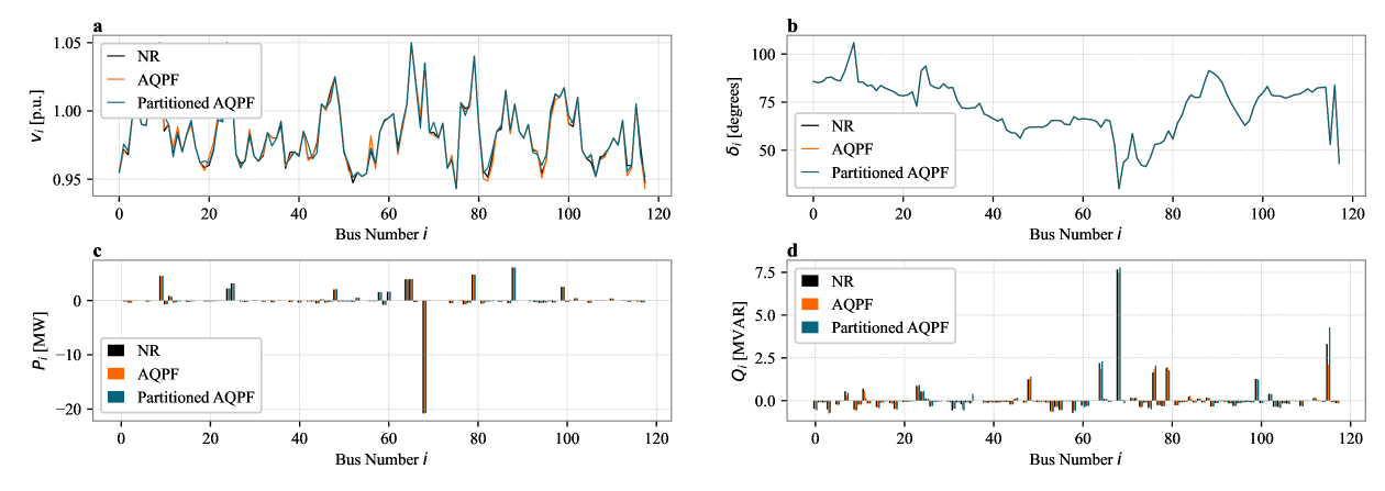
Figure 1: Performance comparison of the Newton-Raphson method (NR), Adiabatic Quantum Power Flow algorithm (AQPF), and partitioned AQPF for the 118-bus test case using Fujitsu’s Quantum-Inspired Integrated Optimization software (QIIO). The results are shown for (a) voltage magnitude $V_{i}\;\text{(p.u.)}$, (b) voltage phase angle $\delta_{i}\;\text{(degrees)}$, (c) net active power $P_{i}\;\text{(MW)}$, and (d) net reactive power $Q_{i}\;\text{(MVAR)}$.

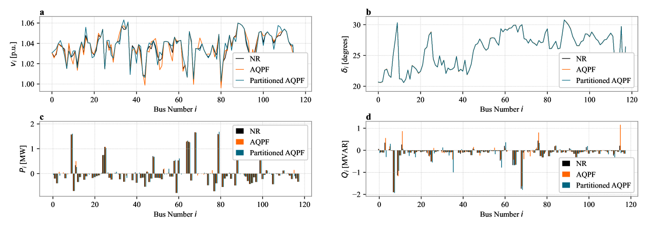
Figure 2: Performance comparison of the Newton-Raphson method (NR), Adiabatic Quantum Optimal Power Flow algorithm (AQOPF), and partitioned AQOPF for the 118-bus test case using Fujitsu’s Quantum-Inspired Integrated Optimization software (QIIO). The results are shown for (a) voltage magnitude $V_{i}\;\text{(p.u.)}$, (b) voltage phase angle $\delta_{i}\;\text{(degrees)}$, (c) net active power $P_{i}\;\text{(MW)}$, and (d) net reactive power $Q_{i}\;\text{(MVAR)}$.

VI-A Partitioned Formulation

To assess the performance of the AQPF and AQOPF algorithms, their results, both in the full and partitioned formulations, are compared against NR for the 118-bus test case. The partitioned formulation is derived by excluding a subset of buses, denoted as $\mathbb{P}$, from the problem Hamiltonian in each iteration. Specifically, in each iteration, a set of 24 buses (approximately $20\%$ of the total buses) is randomly selected and removed from the computation. For PF analysis, this modification is applied in Algorithm 1 by excluding the subset $\mathbb{P}$ from the summation term in 15 at line 19, yielding:

$$\leavevmode\resizebox{413.38667pt}{}{$H_{\text{part}}(\vec{x})=\sum_{i=1\atop i\notin\mathbb{P}}^{N=118}(P_{i}-P_{i}^{G}+P_{i}^{D})^{2}+(Q_{i}-Q_{i}^{G}+Q_{i}^{D})^{2}$}.$$ (35)

For OPF, the same subset $\mathbb{P}$ is excluded from the objective function in 29. This partitioned formulation allows for a reduced problem size per iteration.

VI-A1 Partitioned AQPF

For PF analysis, the partitioned formulation in 35 results in a total of $7105$ binary variables (including $472$ base variables and auxiliary variables, which are introduced to reduce higher-order terms), reducing the variable count by $1775$ compared to the full AQPF algorithm. With a residual threshold of $1\times 10^{-2}$ ${\text{MW}^{2}+\text{MVAR}^{2}}\over 2$, the mean square error (MSE) for the net active power $P_{i}$ between AQPF and NR is $4.28\times 10^{-4}\;\text{MW}^{2}$, while for partitioned AQPF, it is $8.06\times 10^{-4}\;\text{MW}^{2}$. Similarly, the MSE for the net reactive power $Q_{i}$ between AQPF and NR is $1.65\times 10^{-2}\;\text{MVAR}^{2}$, while for partitioned AQPF, it is $1.8\times 10^{-2}\;\text{MVAR}^{2}$. These results, illustrated in Fig. 1, indicate that AQPF closely matches NR, and the partitioned formulation does not significantly degrade solution quality. Further improvements can be achieved by reducing the residual threshold.

In terms of computational performance, AQPF requires $272.98\;\text{s}$ for compilation, compared to $208.34\;\text{s}$ for partitioned AQPF. The average time per iteration is $251.24\;\text{s}$ for AQPF and $217.61\;\text{s}$ for partitioned AQPF. Note that the total computational time includes communication overhead between the classical and quantum-inspired hardware.

VI-A2 Partitioned AQOPF

For OPF, the partitioned formulation reduces the number of binary variables (including $472$ base variables, auxiliary variables, which are introduced to reduce higher-order terms, and slack variables, which are introduced to integrate the constraints) to $8459$, which represents a reduction of $2189$ binary variables compared to the full formulation in 29. With a residual of $1\times 10^{-2}$ ${\text{MW}^{2}+\text{MVAR}^{2}}\over 2$, the MSE for the net active power $P_{i}$ between AQOPF and NR is $8.89\times 10^{-4}\;\text{MW}^{2}$, while for partitioned AQOPF, it is $1.57\times 10^{-3}\;\text{MW}^{2}$. Similarly, the MSE for the net reactive power $Q_{i}$ between AQOPF and NR is $1.68\times 10^{-2}\;\text{MVAR}^{2}$, while for partitioned AQOPF, it is $1.69\times 10^{-2}\;\text{MVAR}^{2}$. The results are presented in Fig. 2.

The compilation times for AQOPF and partitioned AQOPF are $408.35\;\text{s}$ and $318.67\;\text{s}$, respectively. The time per iteration is $384.15\;\text{s}$ for AQOPF and $302.82\;\text{s}$ for partitioned AQOPF. These results indicate that the partitioned formulation can reduce computational time by up to $20\%$ while maintaining equivalent solution accuracy.

VI-B Handling Ill-Conditioned Cases

TABLE II: Comparison of AQPF and AQOPF under well-conditioned and ill-conditioned scenarios for the 118-bus test case.

Scenario	AQPF			AQOPF
	Residual	Mismatch	Mismatch	Residual	Mismatch	Mismatch
	${\text{MW}^{2}+\text{MVAR}^{2}}\over 2$	MW2	MVAR2	${\text{MW}^{2}+\text{MVAR}^{2}}\over 2$	MW2	MVAR2
Well-conditioned case	$8.47\times 10^{-3}$	$4.28\times 10^{-4}$	$1.65\times 10^{-2}$	$8.85\times 10^{-3}$	$8.89\times 10^{-4}$	$1.68\times 10^{-2}$
Ill-conditioned case 1	$8.73\times 10^{-3}$	$5.75\times 10^{-4}$	$1.68\times 10^{-2}$	$8.59\times 10^{-3}$	$8.67\times 10^{-4}$	$1.63\times 10^{-2}$
Ill-conditioned case 2	$8.92\times 10^{-3}$	$5.24\times 10^{-4}$	$1.73\times 10^{-2}$	$8.87\times 10^{-3}$	$7.23\times 10^{-4}$	$1.71\times 10^{-2}$

To simulate challenging operating conditions, two ill-conditioned cases are introduced for the 118-bus test case by modifying system parameters as follows:

1. Load demands at a subset of PQ buses are increased to create stress conditions that exceed the system’s typical operating limits (Ill-conditioned case 1).

2. The resistance ($R$) values of transmission lines connecting a subset of buses are increased, while the reactance ($X$) values remain unchanged. This results in significantly higher $R/X$ ratios and increasing network losses (Ill-conditioned case 2).

Under these ill-conditioned scenarios, the NR solver in pandapower diverges for PF, and for OPF, numerical instability leads to infeasible solutions or failure to converge with optimization constraints remaining unmet. On the other hand, AQPF and AQOPF successfully solve both PF and OPF problems under the same ill-conditioned scenarios. The results are summarized in Table II.

The capability of AQPF and AQOPF in handling ill-conditioned cases is attributed to the enhanced numerical stability, that is, their combinatorial formulation avoids reliance on traditional linearization techniques, and hence mitigates issues caused by near-singular Jacobians. On the other hand, by iteratively refining increments/decrements, the algorithms ensure steady progress toward feasible solutions. The ability of Ising machines to handle a large number of binary decision variables also enables efficient searching of the solution space.

To further investigate the robustness of AQPF under ill-conditioned scenarios, the experiment is extended to include the partitioned AQPF formulation, as defined in 35, to solve PF analysis for the Ill-conditioned case 1. The results show that the partitioned AQPF formulation successfully solves the PF problem even under these challenging conditions. Specifically, the residual is $8.83\times 10^{-3}$ ${\text{MW}^{2}+\text{MVAR}^{2}}\over 2$, and the active and reactive power mismatches are $5.42\times 10^{-4}\;\text{MW}^{2}$ and $1.49\times 10^{-2}\;\text{MVAR}^{2}$, respectively. These results further underscore the capability of the partitioned AQPF approach to maintain computational efficiency without sacrificing solution accuracy, even in ill-conditioned scenarios.

VI-C Scalability

The scalability of the AQPF and AQOPF algorithms is demonstrated by their ability to handle an increasing number of binary variables, as validated through experiments on test cases of varying sizes using QIIO. The results are summarized in Table III and Table IV, respectively; presenting the number of binary variables (-), the time needed to compile the QUBO formulation (s), the time elapsed per iteration (s), and the residual (${\text{MW}^{2}+\text{MVAR}^{2}}\over 2$). Accordingly, QIIO can accommodate the number of binary variables required for solving the PF problem up to the 1354-bus test case and the OPF problem up to the 300-bus test case. However, due to the high computational complexity associated with the larger test cases, only a limited number of iterations are performed for tehm with a residual threshold of $1\times 10^{0}$ ${\text{MW}^{2}+\text{MVAR}^{2}}\over 2$, which serves as a proof of concept.

TABLE III: Scalability of AQPF for different test cases.

Test Case	No. of	Compile	Time per	Residual
	Variables [-]	Time s	Iteration s	${\text{MW}^{2}+\text{MVAR}^{2}}\over 2$
9-bus	$249$	$0.27$	$0.93$	$8.47\times 10^{-3}$
14-bus	$494$	$39.62$	$41.81$	$8.11\times 10^{-3}$
30-bus	$1,183$	$40.35$	$40.91$	$8.52\times 10^{-3}$
57-bus	$3,873$	$90.05$	$65.81$	$8.57\times 10^{-3}$
118-bus	$8,881$	$272.98$	$251.24$	$8.47\times 10^{-3}$
200-bus	$15,098$	$238.22$	$231.07$	$9.38\times 10^{-1}$
300-bus	$23,577$	$896.38$	$926.64$	$8.72\times 10^{-1}$
1354-bus	$99,509$	$43,151.54$	$41,745.91$	$9.67\times 10^{-1}$

TABLE IV: Scalability of AQOPF for different test cases.

Test Case	No. of	Compile	Time per	Residual
	Variables [-]	Time s	Iteration s	${\text{MW}^{2}+\text{MVAR}^{2}}\over 2$
9-bus	$331$	$0.42$	$1.81$	$8.59\times 10^{-3}$
14-bus	$692$	$47.52$	$48.51$	$8.82\times 10^{-3}$
30-bus	$1.537$	$52.11$	$53.78$	$8.73\times 10^{-3}$
57-bus	$6,021$	$108.34$	$96.29$	$8.69\times 10^{-3}$
118-bus	$10,648$	$408.35$	$384.15$	$8.85\times 10^{-3}$
200-bus	$18,571$	$468.08$	$406.65$	$9.84\times 10^{-1}$
300-bus	$29,498$	$1,659.12$	$1,395.87$	$9.79\times 10^{-1}$

VII Discussion

The following observations can be made:

• Due to the high computational cost, the experiments are conducted with a threshold of $1\times 10^{-2}$ ${\text{MW}^{2}+\text{MVAR}^{2}}\over 2$. Given additional computational time, the results could be further refined to obtain higher accuracy.

• D-Wave’s quantum annealer (QA) and hybrid solver (HA) are constrained by embedding challenges and available qubit count, which make them unsuitable for large test cases. While they successfully solve small-scale problems, their applicability to real-world power systems remains limited without improvements in embedding techniques, hardware connectivity, and qubit counts.

• Fujitsu’s Quantum-Inspired Integrated Optimization software (QIIO) offers a remarkable capability of handling up to 100,000 binary variables, making it an excellent platform for realizing large-scale power system problems.

• A more efficient update scheme can significantly enhance the performance of the proposed algorithms by minimizing computational overhead while maintaining accuracy. Future work, therefore, can improve the update scheme to reduce the number of iterations required for convergence.

• The AQPF algorithm can be generalized as a “model of models” approach that is executable on Ising machines. This capability opens avenues for tackling a wide range of problems beyond power systems, particularly those that are computationally challenging for classical solvers.

VIII Conclusion

This study introduces Adiabatic Quantum Power Flow (AQPF) and Adiabatic Quantum Optimal Power Flow (AQOPF) algorithms as novel approaches for, respectively, solving power flow (PF) and optimal power flow (OPF) problems using Ising machines. The feasibility of the proposed algorithms is demonstrated for large-scale power systems, and also their computational efficiency and scalability are highlighted. The findings confirm that the AQPF and AQOPF algorithms consistently achieve convergence across various test cases, including complex and ill-conditioned test cases, where conventional solvers often struggle. The results also suggest that Fujitsu’s Quantum-Inspired Integrated Optimization software (QIIO) offers a compelling alternative to classical solvers, particularly for problems with high-dimensional, combinatorial structures. This research, therefore, marks a significant step toward integrating Ising machines into power system applications but also paves the way for enhanced efficiency, scalability, and robustness in solving large-scale optimization problems.

References

- [1] J. Long, Z. Yang, J. Zhao, and J. Yu, “Modular linear power flow model against large fluctuations,” IEEE Transactions on Power Systems, vol. 39, no. 1, pp. 402–415, 2024.
- [2] F. Capitanescu and L. Wehenkel, “Improving the statement of the corrective security-constrained optimal power-flow problem,” IEEE Transactions on Power Systems, vol. 22, no. 2, pp. 887–889, 2007.
- [3] M. Huneault and F. Galiana, “A survey of the optimal power flow literature,” IEEE Transactions on Power Systems, vol. 6, no. 2, pp. 762–770, 1991.
- [4] Z. Liu, X. Zhang, M. Su, Y. Sun, H. Han, and P. Wang, “Convergence analysis of newton-raphson method in feasible power-flow for dc network,” IEEE Transactions on Power Systems, vol. 35, no. 5, pp. 4100–4103, 2020.
- [5] Z. Liu, R. Liu, X. Zhang, M. Su, Y. Sun, H. Han, and P. Wang, “Further results on newton-raphson method in feasible power-flow for dc distribution networks,” IEEE Transactions on Power Delivery, vol. 37, no. 2, pp. 1348–1351, 2022.
- [6] A. Nur and A. Kaygusuz, “Load flow analysis with newton–raphson and gauss–seidel methods in a hybrid ac/dc system,” IEEE Canadian Journal of Electrical and Computer Engineering, vol. 44, no. 4, pp. 529–536, 2021.
- [7] Y. Liu, K. Sun, and J. Dong, “A dynamized power flow method based on differential transformation,” IEEE Access, vol. 8, pp. 182 441–182 450, 2020.
- [8] A. Ahmadi, M. C. Smith, E. R. Collins, V. Dargahi, and S. Jin, “Fast newton-raphson power flow analysis based on sparse techniques and parallel processing,” IEEE Transactions on Power Systems, vol. 37, no. 3, pp. 1695–1705, 2022.
- [9] N. Costilla-Enriquez, Y. Weng, and B. Zhang, “Combining newton-raphson and stochastic gradient descent for power flow analysis,” IEEE Transactions on Power Systems, vol. 36, no. 1, pp. 514–517, 2021.
- [10] X. Su, C. He, T. Liu, and L. Wu, “Full parallel power flow solution: A gpu-cpu-based vectorization parallelization and sparse techniques for newton–raphson implementation,” IEEE Transactions on Smart Grid, vol. 11, no. 3, pp. 1833–1844, 2020.
- [11] D. Kumari, S. K. Chattopadhyay, and A. Verma, “Improvement of power flow capability by using an alternative power flow controller,” IEEE Transactions on Power Delivery, vol. 35, no. 5, pp. 2353–2362, 2020.
- [12] Z. Kaseb, S. Orfanoudakis, P. P. Vergara, and P. Palensky, “Adaptive informed deep neural networks for power flow analysis,” vol. 235, p. 110677, 10 2024.
- [13] L. Liu, N. Shi, D. Wang, Z. Ma, Z. Wang, M. J. Reno, and J. A. Azzolini, “Voltage calculations in secondary distribution networks via physics-inspired neural network using smart meter data,” IEEE Transactions on Smart Grid, vol. 15, no. 5, pp. 5205–5218, 2024.
- [14] Z. Wu, M. Zhang, S. Gao, Z.-G. Wu, and X. Guan, “Physics-informed reinforcement learning for real-time optimal power flow with renewable energy resources,” IEEE Transactions on Sustainable Energy, vol. 16, pp. 216–226, 1 2024.
- [15] F. Yin, H. Tamura, Y. Furue, M. Konoshima, K. Kanda, and Y. Watanabe, “Extended ising machine with additional non-quadratic cost functions,” Journal of the Physical Society of Japan, vol. 92, 3 2023.
- [16] Z. Kaseb, M. Möller, P. P. Vergara, and P. Palensky, “Power flow analysis using quantum and digital annealers: a discrete combinatorial optimization approach,” Scientific Reports, vol. 14, no. 1, p. 23216, 2024.
- [17] H. Goto, K. Tatsumura, and A. R. Dixon, “Combinatorial optimization by simulating adiabatic bifurcations in nonlinear hamiltonian systems,” Science Advances, vol. 5, 4 2019.
- [18] A. Lucas, “Ising formulations of many np problems,” Frontiers in Physics, vol. 2, 2014.
- [19] P. I. Bunyk, E. M. Hoskinson, M. W. Johnson, E. Tolkacheva, F. Altomare, A. J. Berkley, R. Harris, J. P. Hilton, T. Lanting, A. J. Przybysz, and J. Whittaker, “Architectural considerations in the design of a superconducting quantum annealing processor,” IEEE Transactions on Applied Superconductivity, vol. 24, pp. 1–10, 8 2014.
- [20] H. Goto, K. Endo, M. Suzuki, Y. Sakai, T. Kanao, Y. Hamakawa, R. Hidaka, M. Yamasaki, and K. Tatsumura, “High-performance combinatorial optimization based on classical mechanics,” Science Advances, vol. 7, 2 2021.
- [21] N. Dattani, “Quadratization in discrete optimization and quantum mechanics,” 1 2019.
- [22] Z. Kaseb, M. Möller, M. Kirsch, P. Palensky, and P. P. Vergara, “Combinatorial power flow analysis using adiabatic quantum algorithms,” in 2025 IEEE Belgrade PowerTech, 2025.
- [23] L. Thurner, A. Scheidler, F. Schäfer, J.-H. Menke, J. Dollichon, F. Meier, S. Meinecke, and M. Braun, “pandapower—an open-source python tool for convenient modeling, analysis, and optimization of electric power systems,” IEEE Transactions on Power Systems, vol. 33, no. 6, pp. 6510–6521, 2018.