Super-Resolution with Structured Motion
Abstract
We consider the limits of super-resolution using imaging constraints. Due to various theoretical and practical limitations, reconstruction-based methods have been largely restricted to small increases in resolution. In addition, motion-blur is usually seen as a nuisance that impedes super-resolution. We show that by using high-precision motion information, sparse image priors, and convex optimization, it is possible to increase resolution by large factors. A key operation in super-resolution is deconvolution with a box. In general, convolution with a box is not invertible. However, we obtain perfect reconstructions of sparse signals using convex optimization. We also show that motion blur can be helpful for super-resolution. We demonstrate that using pseudo-random motion it is possible to reconstruct a high-resolution target using a single low-resolution image. We present numerical experiments with simulated data and results with real data captured by a camera mounted on a computer controlled stage.
Index Terms:
Computational Photography, Super-resolution, Compressed Sensing, Deconvolution1 Introduction
We consider the super-resolution problem where the goal is to reconstruct a high-resolution image from one or several low-resolution images. We focus primarily on the use of imaging constraints and low-level image priors, and on the use of motion to capture one or more pictures.
One of our motivations is to implement a compressed sensing system for super-resolution. Using a high-resolution CCD/CMOS sensor, it may be possible to reconstruct an extremely high-resolution image using an appropriate optical and computational imaging system.
Classical reconstruction-based methods relate a collection of low-resolution images to a high-resolution image using a model of the imaging process. Such methods have been largely restricted to small increases in resolution due to theoretical and practical limitations [1, 2]. In addition, motion blur is usually seen as a nuisance that impedes super-resolution [3].
We show that by using multiple static images acquired in a grid of locations and sparse image priors, it is possible to increase resolution by large factors. We note a connection between super-resolution and deconvolution with a box filter, which helps to understand the ambiguities in the super-resolution problem. In particular, the low-resolution images determine most of the Fourier components of the super-resolution image and, in this setting, sparse images can be recovered using convex optimization.
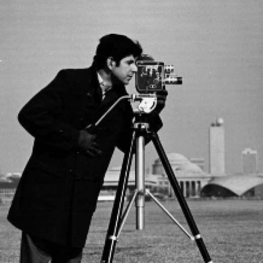
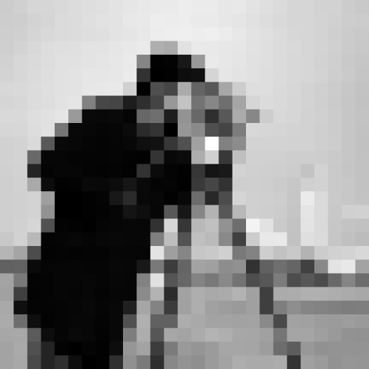
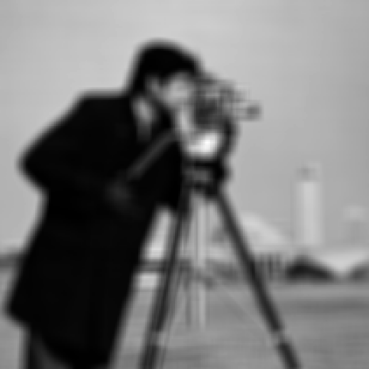
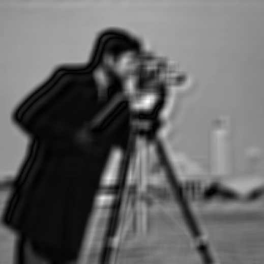
We also show that by using pseudorandom motion it may be possible to reconstruct a high-resolution target using a single low-resolution image. Figure 1 illustrates this idea. In this case, we capture an image while the camera/sensor undergoes a large vibration. By solving a convex optimization problem with the imaging constraints and sparsity prior, we obtain an essentially perfect reconstruction of the high-resolution target from a single low-resolution image.
 |
 |
 |
 |
| Ground truth | Sensor trajectory | Recorded image | Reconstruction |
Super-resolution imaging systems have many potential applications. In some settings, there are practical and physical limitations that lead to low-resolution sensors. For the case of visible light photography with high-resolution sensors, our methods could be used to produce gigapixel images using a small camera. High-resolution imaging has many applications in science and in archival/preservation work (including for art, documents, and biological samples). Furthermore, there are many applications where a camera might be constantly moving, such as in aerial imaging.
We implemented a system to demonstrate some of our ideas using a commonly available camera and computer controlled motion stage. The experiments in Section 6 demonstrate results using both static images and images taken with the camera moving at constant velocity.
Throughout the paper, we focus on cases where the effective resolution is limited by the sensor and not by the optical path (diffraction). Even with high-resolution sensors, super-resolution can be useful for obtaining a wider field of view with an appropriate lens. The interlacing operation described in Section 6.2 is reminiscent of a panorama, but interlaces a set of pictures taken with small motion instead of tiling pictures taken with large motion, which leads to a more compact design for a high-resolution camera. The Wiener filter approach for reconstruction is very efficient and yields a significant improvement in resolution in our experiments. In practice, large images can also be processed in parallel via tiling.
We assume throughout the paper that the sensor motion is known, either because it is carefully planned and executed by a high-accuracy actuator or because we have a high-accuracy readout of the sensor position while it is being moved through some other means (such as vibration). For the experiments in Section 6.3, we estimate the camera trajectory during an exposure using a landmark.
2 Related Work
The super-resolution problem has a long history (see, e.g.[4, 5, 1, 2]). From a theoretical point of view, the results in [1] and [2] are largely negative, showing that ambiguity in the super-resolution problem grows quickly with the desired increase in resolution. In contrast, here we note that with a particular sampling scheme this ambiguity is concentrated on relatively few Fourier coefficients. Previous work in compressed sensing [6, 7] has shown that sparse image priors can be used to resolve such ambiguities.
[3] proposed the use of a ”Jitter camera” to improve the resolution of video by quickly moving the sensor in the imaging plane of a camera without introducing motion blur, which was believed to impede super-resolution. Here we argue that motion blur can in fact aid in super-resolution.
Intuitively, the combination of motion blur and discrete sampling can be used to define a compressed sensing system. The approach is related to the use of random filters for compressed sensing [8, 9].
A variety of unique imaging system designs have been developed through the use of compressed sensing methods. Some physical implementations include [10, 11, 12].
Recently, some imaging schemes have been proposed, not to achieve super-resolution, but to remove motion-related artifacts. For example, parabolic lens motion [13], induced by constant acceleration, generates a PSF that is invariant to object velocity. Additionally, coded blur generated by fluttering a camera shutter [14, 15] has been shown to help in removing motion blur. This leads to a surprising idea that it may be beneficial to extend an exposure with a coded shutter to compensate for motion blur.
Many super-resolution methods use training data or other sources of information to improve image resolution. The idea of exemplar based super-resolution goes back to the work in [1] and was implemented at a large scale in [16]. Generic image priors based on self-similarity have also been used for super-resolution [17]. More recent methods have used deep neural networks for super-resolution from a single image[18].
In this paper, we focus on the use of total variation for reconstruction. In practice, alternative image priors, such as ones based on self-similarity or deep networks, could also be implemented using Plug-and-Play methods [19].
Neural models have been increasingly used for image reconstruction, including super-resolution [20]. The use of a neural radiance field (NeRF) allows for the estimation of a continuous image instead of selecting a particular target resolution. In this case, one can implement the imaging model described here by Monte Carlo integration via sampling a finite number of locations in the imaging plane.
We consider only grayscale images to simplify the presentation and experimental design. For the case of color images captured with a color filter array, one could reconstruct a super-resolution image for each color channel separately, using measurements defined by pixels of that color in the filter array. This is related to the recent approach in [21] which performs super-resolution without explicit demosaicing. By using controlled motion, one can also collect measurements for every pixel using each color in the filter array.
3 Imaging Model
Our goal is to reconstruct a high-resolution image from one or several low-resolution images. In the mathematical model we consider here, the low-resolution images are captured with a sensor that can translate in the imaging plane of a camera. In one setting, we capture a series of images in a grid of high-resolution (sub-pixel) locations. In another setting, we capture one or more images while the sensor is moving; for example, we can record a single or sequence of pictures while vibrating the sensor or moving along a linear trajectory (e.g, as may be the case in satellite imaging).
There are many equivalent practical situations. In the experiments in Section 6, we use a standard camera on a moving stage, which is equivalent to moving the sensor when viewing a planar object parallel to the camera. In a microscope, instead of moving the sensor, we can precisely move the sample using a piezo nanopositioning stage.
Let denote a continuous brightness function in the imaging plane of a camera. We do not model the optics of the camera and focus only on measuring the image projected onto the imaging plane.
An sensor integrates over square pixels tiling a rectangular area. We use to denote the side length of a pixel in the sensor. Each pixel integrates the light that falls in a particular square region over a unit of time.
Ignoring measurement noise, if we place the sensor in the imaging plane with bottom-left corner at we capture a discrete image with
We will also consider the case where the sensor moves while the image is captured. If the sensor follows a trajectory , we capture an image with
Note that translating the sensor by is equivalent to translating by . Let denote the occupancy map defined by the trajectory . The image captured by the moving sensor is equal the image of captured by a static sensor.
We consider methods that increase the resolution of the camera sensor to generate a super-resolution image that would have been recorded by a static sensor with pixels of size for an integer factor defining the resolution increase. This virtual sensor covers an area that is at least as big as the camera sensor and the image has at least pixels (the area may be larger due to the sensor motion). In our experiments, we have used super-resolution factors as high as .
4 Grid of Images
Let be an image generated by a (virtual) sensor with pixel size at the origin. Let be an image captured by a (physical) sensor with pixel size at where
with and integers. In this case, the low-resolution pixels in are aligned with the high-resolution pixels in . In particular, each value in is the sum of values in ,
We see that is a decimation (subsampling) of where is a two-dimensional box filter of width .
Suppose we capture different low-resolution images by translating the sensor over an grid of high-resolution locations,
Capturing such images involves moving the sensor to sub-pixel locations defined with a step size . The total vertical and horizontal displacement required to capture all images is less than .
4.1 Interlacing
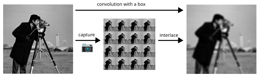
The different images can be rearranged into a single image such that , where is a box of width . Since each image is a decimation of , the rearrangement interlaces the captured images:
Figure 2 illustrates the process where we capture multiple low-resolution images and interlace the result to obtain a single “blurry” image . The interlaced image has pixels and defines the imaging constraints on through the relation .
4.2 Deconvolution with a Box
Recovering the super-resolution image is equivalent to a deconvolution of with a two-dimensional box filter of width . That is, we need to de-blur to recover .
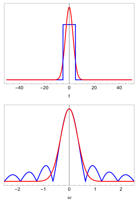
Note that a box filter is not a good smoothing or low-pass filter. Convolution with a box wields a signal that is visually blurry but still has quite a lot of high-frequency information. In Figure 3(a) we compare the Fourier transform of a one-dimensional box and a Gaussian of similar width. The Fourier transform of a Gaussian is a Gaussian and the Fourier transform of a box is a sinc. In particular, the magnitude of the Fourier transform of the box decays much slower than the magnitude of the Fourier transform of a Gaussian.
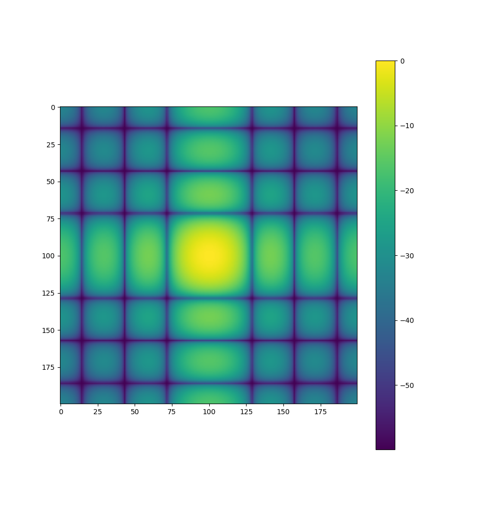
For the case of a two-dimensional discrete (periodic) signal, we illustrate the magnitude of the DFT of when in Figure 3(b). Note that there are relatively few coefficients in the DFT of with magnitude close to 0. We can therefore directly recover most of the coefficients in the Fourier transform of from the Fourier transform of , except for isolated frequencies where the Fourier transform of is zero or close to zero.
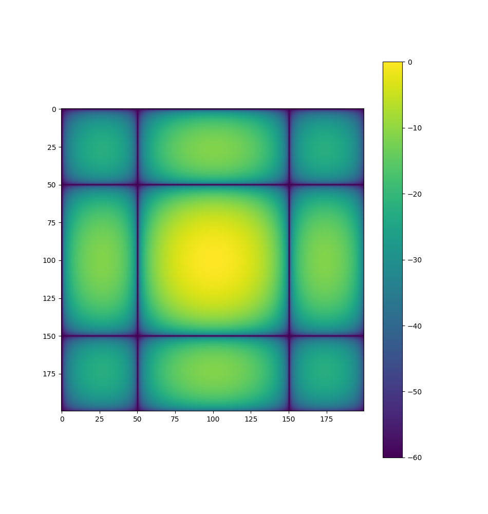
Previous work [1, 2] showed that the ambiguity in grows exponentially with . We note, however, that even for large factors , the constraints defined by identify most of the Fourier coefficients of .
The number of times the Fourier transform of a discrete periodic box of width crosses zero is . Therefore, the ambiguity in is concentrated on relatively few Fourier coefficients. In this setting, sparse image priors and convex optimization are known to yield surprisingly good reconstructions [6, 7].
For the specific case of deconvolution with a box, we have shown [22] that convex optimization using regularization can lead to perfect reconstruction of sparse one-dimensional signals.
Figure 4 illustrates a numerical experiment with a simulated camera. The deconvolution of using a total variation prior yields an almost perfect reconstruction including very high-resolution details.
4.3 Wiener Deconvolution
Using a Gaussian prior on the Fourier coefficients of leads to a fast Wiener deconvolution algorithm via the FFT and an inverse transform. The result corresponds to a MAP estimate of the super-resolution image . The prior is defined by a single parameter used to shrink the estimated Fourier coefficients.
4.4 Sparse Reconstruction
As mentioned above, previous work has shown that sparse signals can often be recovered from incomplete frequency information [6, 7].
In practice, we regularize the reconstruction of the super-resolution image using the total variation (TV) measure, which leads to a convex optimization problem,
where is the total-variation of ,
and is a regularization parameter.
5 Super-resolution by Deblurring
In the previous section, we considered the case of multiple static images taken from different sensor locations. Here we consider the case where one or more images are captured while the sensor is moving.
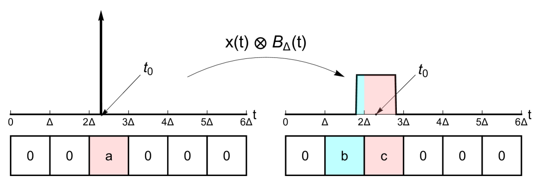
First, we note that a small amount of motion blur can be helpful for super-resolution. Consider the problem of localizing a point source in one dimension; without motion, we can only localize the point source to the pixel size. Now suppose we move the sensor/camera with constant velocity by one pixel while taking a picture. Figure 5 illustrates this situation. The point source is spread over two pixels and we observe two non-zero values and . Together, these measurements determine both the total light intensity and the precise point source location,
Optical blurring, such as due to diffraction, can lead to a similar effect (see, e.g.[23]) but the use of motion may have advantages since, as discussed in the previous section, convolution with a box preserves more information when compared to a Gaussian filter of similar width.
We also note that for “sparse” scenes, we can use large motions to (in essence) take multiple low-resolution images in different areas of the sensor. Shown below in Figure 6 is a simulation where we vibrate a sensor while capturing an image, which leads to the somewhat counterintuitive notion that shaking the camera during an exposure can lead to sharper pictures.
Being able to take pictures while the sensor/camera is moving allows for faster acquisitions, which is often important. In this case, there is no need to wait for the sensor to move and stabilize in one position before taking a picture; instead, we can follow a continuous trajectory and take a sequence of pictures along the way.
As in the previous section, let be a super-resolution image generated by a virtual sensor at the origin. Now we let be an image captured by a moving sensor. Let for denote the trajectory of the sensor over the grid of high-resolution pixel locations. That is, at time , the sensor is at location .
Let be the occupancy map of . That is, is the total fraction of time this trajectory spends at location . When the sensor undergoes a continuous trajectory we use linear interpolation to define a discrete occupancy map . Let be a box of width . The relationship between and is captured by a decimation by factor of the sequential convolution of with and . The convolution of with accounts for the sensor motion, while the convolution with and decimation accounts for the relative size of the physical and virtual pixels.
Let denote the decimation of by a factor . The imaging constraints are summarized by the linear system,
This system of equations has many fewer constraints than variables, but it can lead to perfect reconstructions with an appropriate image prior as we demonstrate in simulations below.
In some applications we may have a sequence of low-resolution images taken over one or multiple trajectories. Let denote the occupancy map of the trajectory followed during the acquisition of .
We can reconstruct a single super-resolution image using the data from multiple trajectories and a sparsity prior. To estimate a sparse image image use regularization,
Similarly we can regularize the reconstruction using TV,
Here again is a regularization parameter.


5.1 Simulations
We evaluate the quality of the reconstructions obtained using a single exposure when the sensor moves in different trajectories.
Figure 6(a) shows two examples of the high-resolution targets we used for the experiments. Each target is a image with several random characters placed in random locations. Figure 6(b) shows the results of taking a low-resolution picture of each target using a sensor. In this case, there is no sensor motion. We can see that with such a low-resolution picture, the characters become completely unreadable.
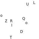
Figure 6(c) shows the results of imaging the two targets from Figure 6(a) with a moving sensor. In each case, the sensor undergoes a large motion. Figure 6(d) shows the reconstructions of the targets from a single low-resolution image, captured while the sensor is moving. In these examples, we obtain a perfect super-resolution image from a single low-resolution image by leveraging motion blur.
For the experiments in this section, we treat the high-resolution target as periodic. The sensor motion therefore leads to a cyclic convolution between the target and the sensor occupancy map. We used the norm of the target image to regularize the reconstructions.
We consider the following trajectories for the sensor:
-
1.
1000 random displacements (shifts). In this case, the trajectory is a sequence of 1000 random locations. Each location is selected independently from a uniform distribution in the high-resolution grid.
-
2.
Random walk with 1000 steps (walk). In this case, the sensor undergoes a random walk in the grid of high-resolution locations.
-
3.
Vibration (vibration). The and coordinates of the sensor are defined by two sinusoidals.
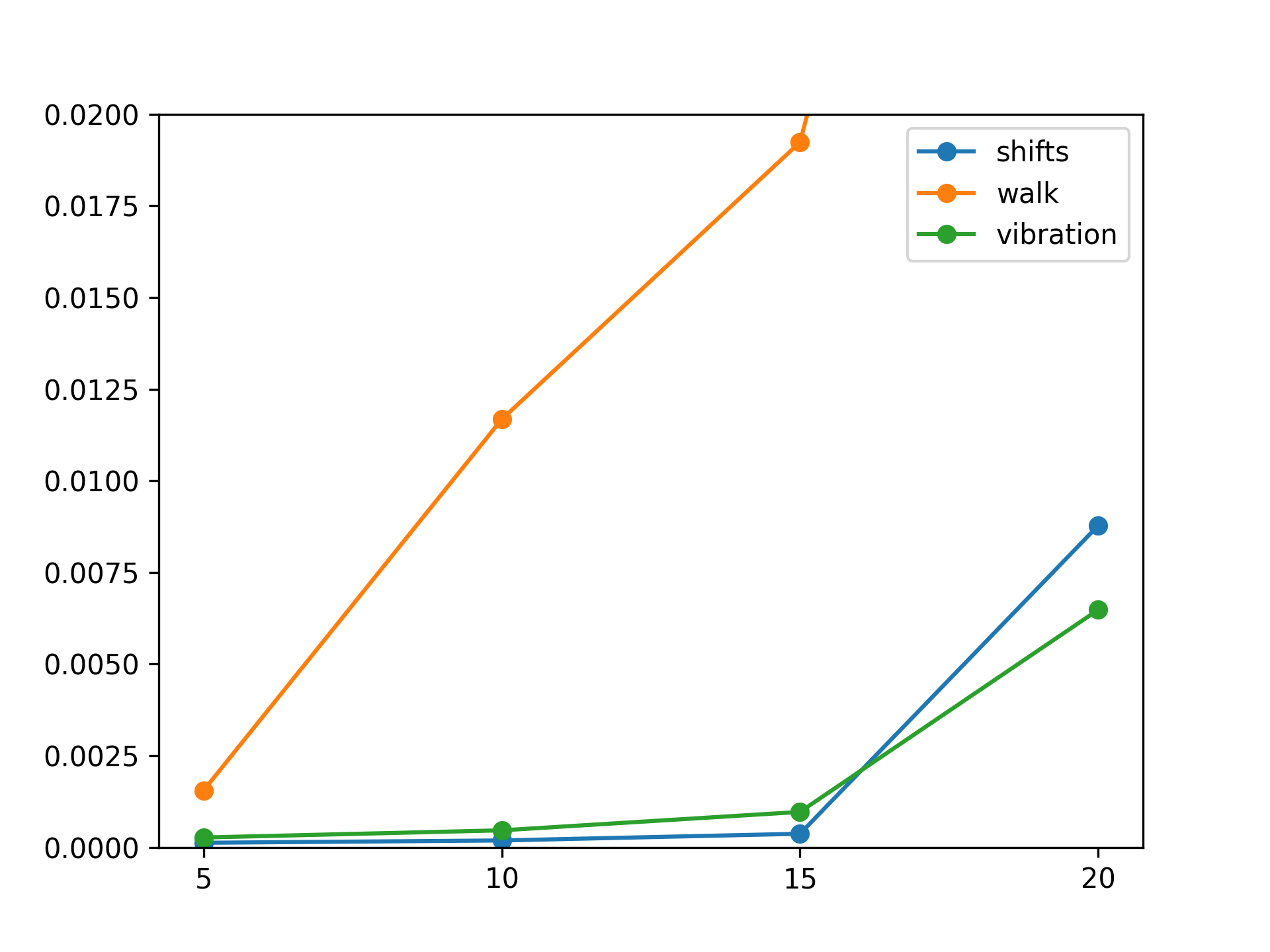
Figure 7 shows the mean RMS error obtained with each trajectory for targets of increasing complexity. We see that for sparse targets, where the number of characters in the image is small, it is possible to obtain perfect 128x128 images using a single 32x32 blurry picture.
6 Experimental Results
We implemented the deconvolution algorithms in python using numpy for the Wiener deconvolution method and both cvxpy and pylops for computing reconstructions using sparsity priors. We found that using the OSQP solver within cvxpy yields good results with small images, as seen in the simulations throughout the paper. For the experiments with real data, we used the split-bregman algorithm implemented in pylops due to the computational demands of processing larger images.
All of the experiments were done with a desktop computer with a 13th Gen Intel(R) Core(TM) i5-13400F CPU with 16 cores and 32GB of RAM.
When , reconstructing a 1200x1520 image from 64 separate 150x190 low-resolution images with the Wiener deconvolution algorithm took about 0.4 seconds. Computing a TV reconstruction using pylops with the same data took between 5 and 10 minutes depending on various tolerances and algorithm parameters.
6.1 Setup
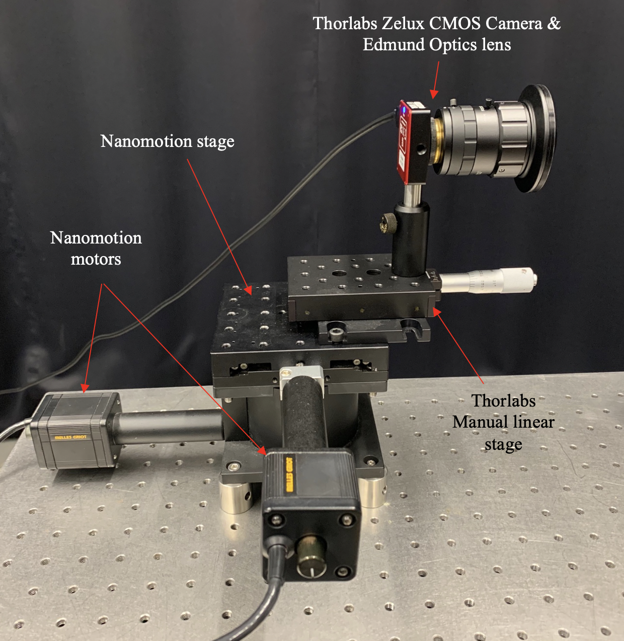
The data used in the following reconstructions consists of sets of images captured by a monochrome 1.6 megapixel (1440x1080) CMOS camera (Thorlabs Zelux) with 3.45 m square pixels and a wide-angle 8 mm f1.8 Edmund Optics lens opened to maximum aperture and focused at approximately 3 meters. This particular choice of lens and sensor leads to an optical system that is not diffraction limited despite the relatively small pixel size.
The camera was mounted on a movable stage and controlled by a nanopositioning system (Nanomotion II) that uses dc stepper motors to move the stage at nanometer level resolution in two separately controlled axes. Movements made by the stage have high precision and repeatability, though no position readout is available. The stage is connected to and controlled by a computer via a serial port.
A static platform was mounted 3 meters away and parallel to the camera to hold targets to be imaged. The illumination source was a battery powered LED tube light (10 inch PavoTubeII 6C RGBWW).
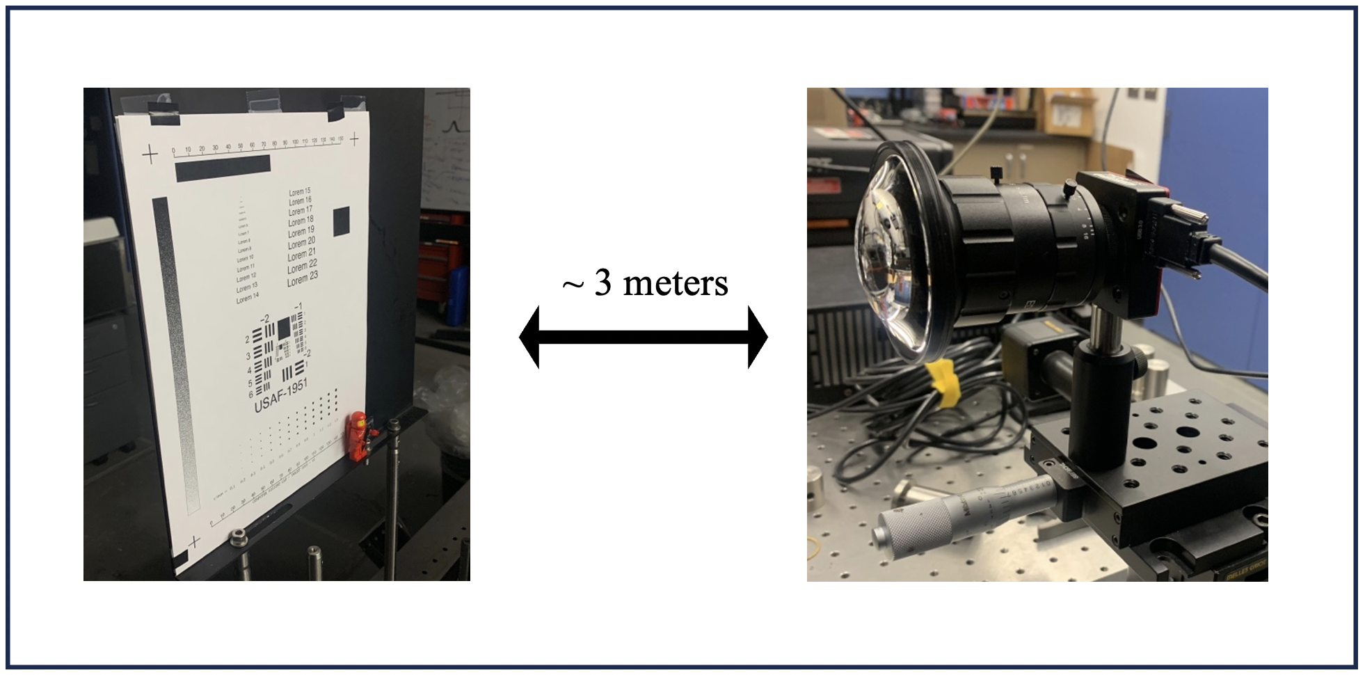
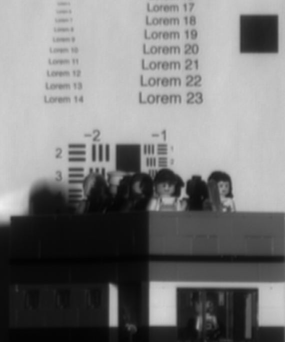
We imaged a variety of targets including small three-dimensional objects (ex. Ketchup packet and LEGO(R) sets) and multiple 8.5” x 11” pages of paper containing designs printed by a standard black and white laser printer, such as a page of text and a to-scale version of the 1951 USAF resolution target.
The USAF target is a standard test chart used to determine the resolution of an optical system. It consists of vertical and horizontal sets of three bars at varying sizes and spatial frequencies that are organized in numbered groups, each with six labeled sets. Once imaged, intensity profiles across the bars can be analyzed; past the resolution limit, three distinct peaks/valleys will no longer be visible in the profile. The group and element number of the smallest resolvable set is used to look up the width and spacing of these bars, and this value, in micrometers or lp/mm, is a measure of the resolution of the system.
For each set of experiments, flat-field images were acquired by imaging a blank sheet of paper, which served as the background for all targets.
6.2 Grid Exposures
In our setup we move the camera instead of the sensor. To acquire a static grid of images, the stage was moved through a series of positions in a plane parallel to the target, coming to a stop at each position and waiting for two frames to be captured, before continuing. The overall grid motion was repeated five times. Averaging many frames reduces the effects of sensor noise and running multiple trials of the grid sequence minimizes the effects of temporal illumination variation during the acquisition.
The number of acquired low-resolution images is determined by the desired resolution increase factor . The actual position of these acquired images depends on the magnification factor induced by the camera optics and the distance to the target.
Moving the camera is equivalent to moving the target, and the magnification of the system relates the distance traveled by the camera to the distance traveled by the image on the sensor. We can determine using the optical properties of the camera and the distance to the target. In practice, we find by imaging an object with known length and calculating its size on the sensor by counting the number of pixels it spans and multiplying by the pixel size.
With grid capture (see Section 6.2), the image of the target moves by less than in both the vertical and horizontal directions, with pictures taken at sub-pixel positions, for a total of image locations. Taking into account the magnification , the distance the stage travels between neighboring grid positions, i.e. step size, is .
For , we use 64 grid locations. The magnification of our system was calculated to be 0.002484 (we use a wide-angle lens), which gives a step size of 0.17361 mm.
Due to the large field of view of the camera, our targets occupy a relatively small (150x190) area in the images acquired, which means that for the experiments presented here, we are only using a small region of the physical sensor in the camera. In other applications, the same setup would allow for capturing very wide field of views.
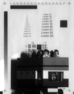
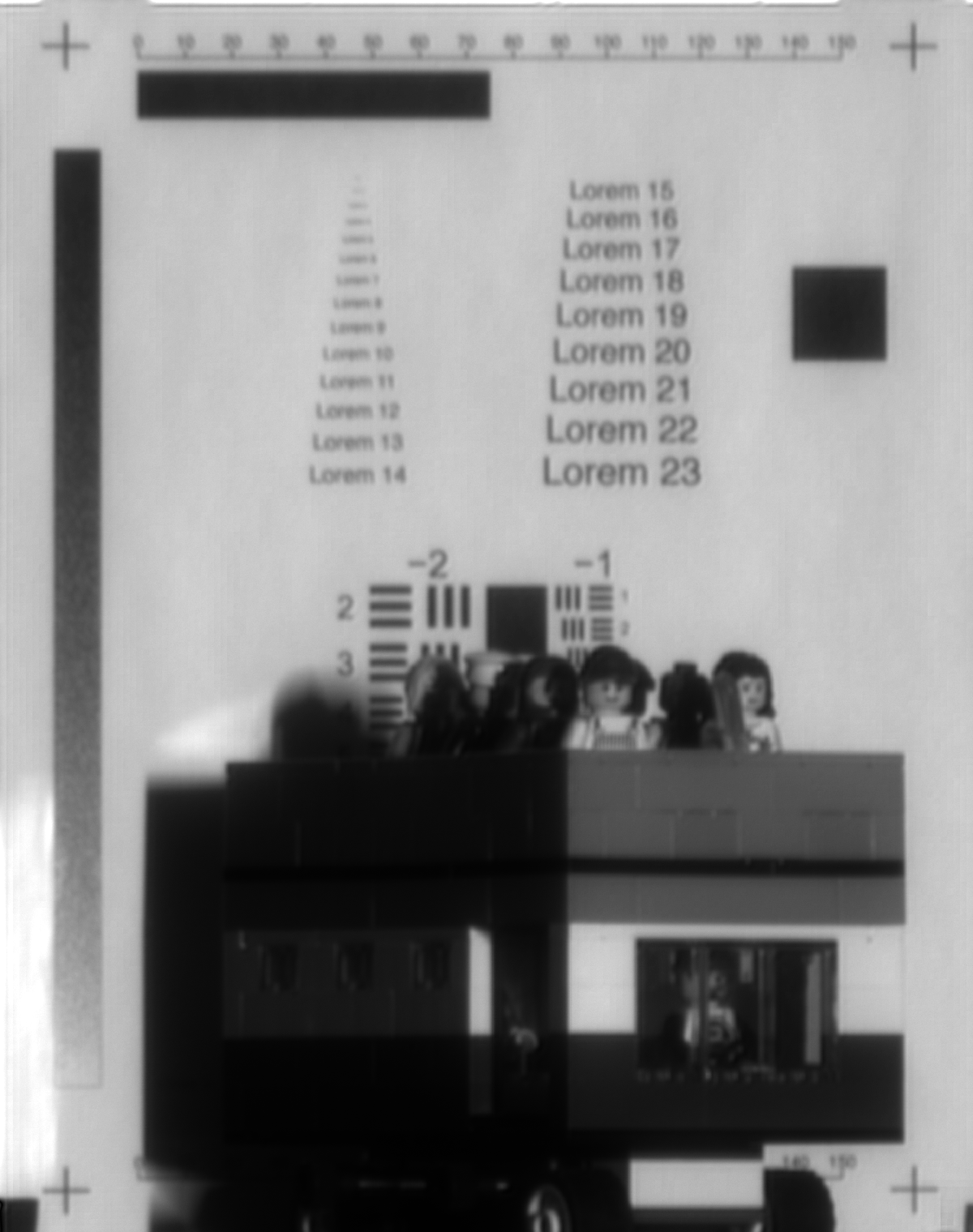
Figure 9 shows several results, each a small ROI of the target area. We note that in each example we can see high-resolution details appear in the super-resolution images (e.g. punctuation and to some extent serifs, elements in USAF group -1, the serrated top edge of the ketchup packet).
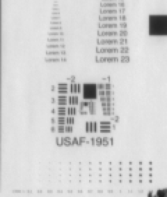
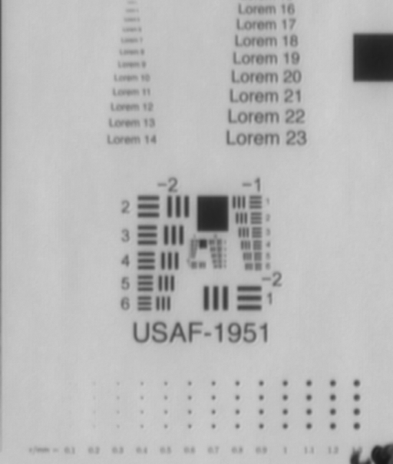
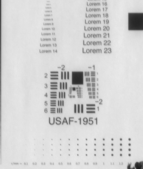
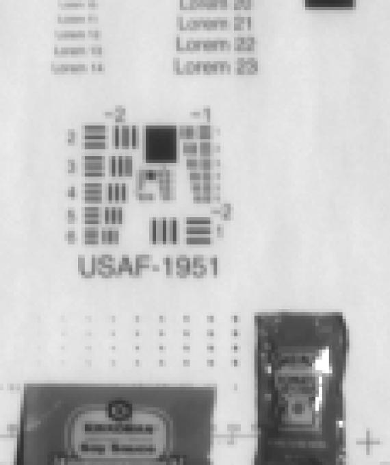
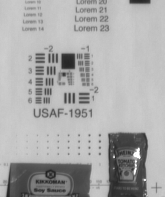

Figure 10 shows that our magnification model holds for three-dimensional objects that protrude out of the target plane. The front of the LEGO(R) bus is approximately 15 cm away from the calibrated target plane and high-resolution details on the minifigures are still resolved.

6.3 Scan Motion
To acquire images with motion, the stage was moved at constant horizontal velocity over a “long” travel range corresponding to a length of many pixels. As the stage moved, five images were captured with a short random delay set before the start of each acquisition. Once the motion across the row was completed, the height of the stage was increased by sub-pixel steps (same as in grid exposures) and the motion was repeated. The total number of heights corresponds to the selected factor .
Since our stage is slow, we used a relatively long exposure to capture images with motion blur. The exposure was determined by how long it takes for the image on the sensor to move by (the size of the sensor pixel). The maximum velocity of the stage is only 2.5 mm/s and therefore, for these experiments we used an exposure time of about five hundred milliseconds.
Due to the fact that the stage has no position readout capabilities and the camera cannot be synchronized with it, the initial camera position for each acquisition must be estimated. The printed targets include a black rectangle, which provides a step edge that is used for the position estimation; similar to the blurred point source shown in Figure 5, a sharp edge can be used for localization. The exposure time, vertical position, and velocity of the stage during each capture are known, so once the initial position has been estimated, the trajectory of motion during the acquisition is fully defined.
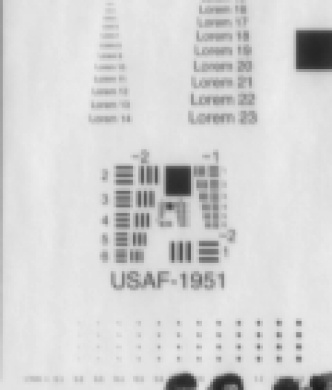
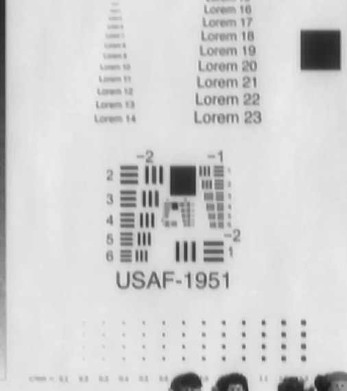
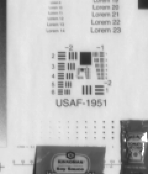
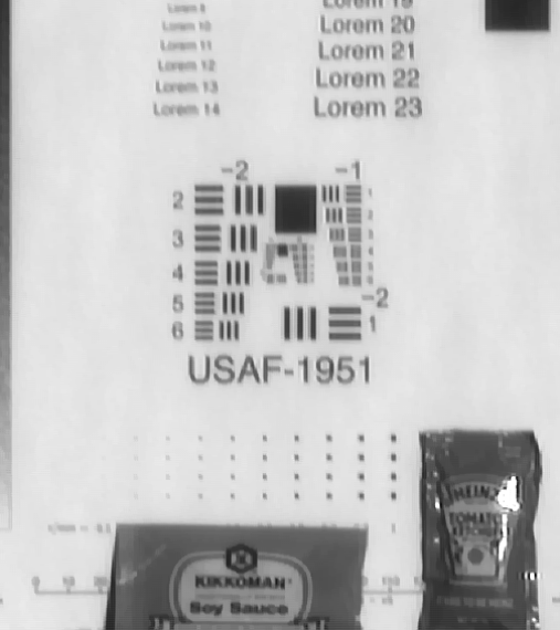
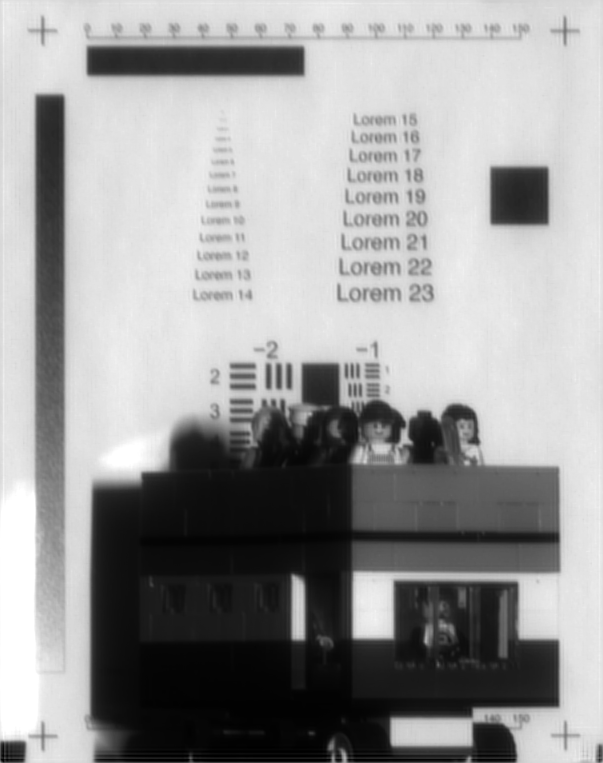
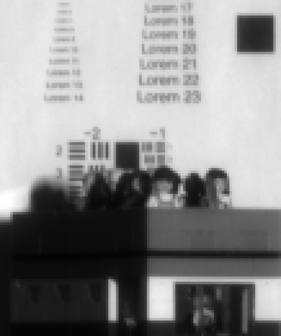
Figure 11 illustrates some results of the scanning motion procedure. These examples demonstrate the use of a moving camera to increase resolution beyond what is visible in a static image, despite the induced motion blur.
7 Conclusion and Future Work
We described several methods for increasing the limits of super-resolution with a moving sensor/camera.
Using a grid of static images, the ambiguity in super-resolution is restricted to relatively few Fourier coefficients. This enables fast reconstruction using a Wiener filter, and higher effective super-resolution factors with sparse priors and compressed sensing techniques.
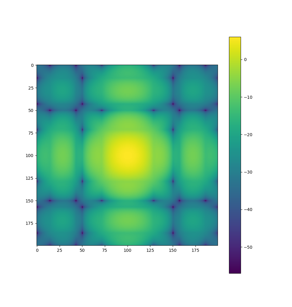
Note that by using two different magnifications during acquisition, or a sensor with multiple pixel sizes, one could potentially remove all of the ambiguity in the super-resolution problem. Figure 12 illustrates the Fourier transform of a discrete periodic box of width 4 and similarly of a box of width 7. We see that the zeros of the two Fourier transforms occur in different places; if we were to record the convolution of a high-resolution image with boxes of two sizes, we would eliminate essentially all ambiguity in the super-resolution problem. Taking pictures while moving at different speeds could also be used to integrate the brightness function over regions of different sizes.
We have also shown that motion blur can in fact be used improve the resolution with a single image. This leads to the idea that to take a sharper picture one should shake or vibrate the camera. In synthetic experiments, we have shown that simply vibrating the image sensor during capture can lead to higher resolution images. The key here is that we solve a motion deblurring problem at the same time that we increase the image resolution, which can be accomplished as long as we have high-resolution trajectory information.
References
- [1] S. Baker and T. Kanade, “Limits on super-resolution and how to break them,” IEEE transactions on pattern analysis and machine intelligence, vol. 24, no. 9, pp. 1167–1183, 2002.
- [2] Z. Lin and H.-Y. Shum, “Fundamental limits of reconstruction-based superresolution algorithms under local translation,” IEEE transactions on pattern analysis and machine intelligence, vol. 26, no. 1, pp. 83–97, 2004.
- [3] M. Ben-Ezra, A. Zomet, and S. K. Nayar, “Jitter camera: High resolution video from a low resolution detector,” in Proceedings of the 2004 IEEE Computer Society Conference on Computer Vision and Pattern Recognition, vol. 2.
- [4] M. Irani and S. Peleg, “Super resolution from image sequences,” in Proceedings. 10th International Conference on Pattern Recognition, vol. 2. IEEE, 1990, pp. 115–120.
- [5] D. Capel and A. Zisserman, “Super-resolution enhancement of text image sequences,” in Proceedings: 15th International Conference on Pattern Recognition. IEEE, 2000.
- [6] E. J. Candès, J. Romberg, and T. Tao, “Robust uncertainty principles: Exact signal reconstruction from highly incomplete frequency information,” IEEE Transactions on information theory, vol. 52, no. 2, pp. 489–509, 2006.
- [7] D. L. Donoho and P. B. Stark, “Uncertainty principles and signal recovery,” SIAM Journal on Applied Mathematics, vol. 49, no. 3, pp. 906–931, 1989.
- [8] J. Romberg, “Compressive sensing by random convolution,” SIAM Journal on Imaging Sciences, vol. 2, no. 4, pp. 1098–1128, 2009.
- [9] J. A. Tropp, M. B. Wakin, M. F. Duarte, D. Baron, and R. G. Baraniuk, “Random filters for compressive sampling and reconstruction,” in 2006 IEEE International Conference on Acoustics Speech and Signal Processing Proceedings, vol. 3.
- [10] R. Fergus, A. Torralba, and W. T. Freeman, “Random lens imaging,” Massachusetts Institute of Technology Computer Science and Artificial Intelligence Laboratory, Tech. Rep., 2006.
- [11] N. Antipa, G. Kuo, R. Heckel, B. Mildenhall, E. Bostan, R. Ng, and L. Waller, “DiffuserCam: lensless single-exposure 3d imaging,” Optica, vol. 5, no. 1, pp. 1–9, 2017.
- [12] M. F. Duarte, M. A. Davenport, D. Takhar, J. N. Laska, T. Sun, K. F. Kelly, and R. G. Baraniuk, “Single-pixel imaging via compressive sampling,” IEEE signal processing magazine, vol. 25, no. 2, pp. 83–91, 2008.
- [13] A. Levin, P. Sand, T. S. Cho, F. Durand, and W. T. Freeman, “Motion-invariant photography,” ACM Transactions on Graphics, vol. 27, no. 3, pp. 1–9, 2008.
- [14] R. Raskar, A. Agrawal, and J. Tumblin, “Coded exposure photography: motion deblurring using fluttered shutter,” ACM Transactions on Graphics, vol. 25, no. 3, pp. 795–804, 2006.
- [15] Y. Tendero, J.-M. Morel, and B. Rougé, “The flutter shutter paradox,” SIAM Journal on Imaging Sciences, vol. 6, no. 2, pp. 813–847, 2013.
- [16] L. Sun and J. Hays, “Super-resolution from internet-scale scene matching,” in 2012 IEEE International conference on computational photography, pp. 1–12.
- [17] D. Glasner, S. Bagon, and M. Irani, “Super-resolution from a single image,” in 12th international conference on computer vision. IEEE, 2009, pp. 349–356.
- [18] C. Dong, C. C. Loy, K. He, and X. Tang, “Image super-resolution using deep convolutional networks,” IEEE transactions on pattern analysis and machine intelligence, vol. 38, no. 2, pp. 295–307, 2015.
- [19] U. S. Kamilov, C. A. Bouman, G. T. Buzzard, and B. Wohlberg, “Plug-and-play methods for integrating physical and learned models in computational imaging: Theory, algorithms, and applications,” IEEE Signal Processing Magazine, vol. 40, no. 1, pp. 85–97, 2023.
- [20] Y. Xie, T. Takikawa, S. Saito, O. Litany, S. Yan, N. Khan, F. Tombari, J. Tompkin, V. Sitzmann, and S. Sridhar, “Neural fields in visual computing and beyond,” in Computer Graphics Forum, vol. 41. Wiley Online Library, 2022, pp. 641–676, issue: 2.
- [21] B. Wronski, I. Garcia-Dorado, M. Ernst, D. Kelly, M. Krainin, C.-K. Liang, M. Levoy, and P. Milanfar, “Handheld multi-frame super-resolution,” ACM Transactions on Graphics, vol. 38, no. 4, pp. 1–18, 2019.
- [22] P. Felzenszwalb, “Deconvolution with a box,” Tech. Rep. arXiv:2407.11685, 2024.
- [23] G. Schiebinger, E. Robeva, and B. Recht, “Superresolution without separation,” Information and Inference: A Journal of the IMA, vol. 7, no. 1, pp. 1–30, 2018.