Human Workload Prediction: Lag Horizon Selection

Abstract

[Figures/SensorsLettersAbstractImage] Human-robot teams must be aware of human workload when operating in uncertain, dynamic environments. Prior work employed physiological response metrics from wearable sensors to estimate the current human workload ; however, these estimates only enable robots to respond to under- or overload conditions reactively. Current human workload prediction approaches are limited to short prediction horizons and fail to investigate variable lag horizons’ impact on predictions. This letter investigates the impact of lag horizons on both univariate and multivariate time series forecasting models for human workload prediction. A key finding is that univariate predictions required longer lag horizons of 240 seconds (s), whereas multivariate workload predictions sufficed with shorter lag horizons with diminishing returns around 120s.

Workload forecasting, Physiological sensors, Time series forecasting

This work has been submitted to the IEEE for possible publication. Copyright may be transferred without notice, after which this version may no longer be accessible.

1 Introduction

Workload represents the ratio between the resource a task requires, and the human’s available resources to dedicate to the task [1]. Task demand exceeding the human’s available resources may overload the human, whereas insufficient task demand may lead to human disengagement (i.e., underload), both of which can negatively impact team performance [2]. Human-robot teams in unstructured, dynamic, and uncertain environments (e.g., disaster response) will result in variable workload, which may decrease team performance. Robots aware of the human’s comprehensive overall workload (i.e., the cognitive, auditory, speech, visual, gross motor, fine motor, and tactile components) may act to address suboptimal workload states. Human workload estimation may be provided by physiological response metrics collected by worn sensors [3]; however, these workload estimates only enable reactive actions. Predictive workload models can be used to preempt negative workload states. These workload predictions must allow sufficient time for a robot to plan and implement adaptations, with longer predictions enabling more complex actions.

Current workload prediction methods only focus on cognitive workload [4, 5, 6, 7, 8, 9]. Up to 30 second (s) workload predictions were made using prior workload values [10, 9], historical task loads [10, 6], physiological response metrics [7, 8, 9], and performance metrics [5] as model predictors. However, these methods only predict a single workload component, have very short prediction horizons (i.e., generally $<5$s), and do not investigate the impact of varying lag horizons. Deciding which lag horizon to use for workload prediction remains an open question [4].

The duration of historical data used for predictions is the lag horizon, and the prediction horizon is the future time point predicted. Longer lag horizons may result in more accurate and longer duration predictions; however, a minimum length lag horizon is desired to enable more computationally efficient models, and to avoid overtraining on the dataset. Prediction accuracy may be influenced by time series data trends (i.e., long term fluctuations), and seasonality (i.e., fixed patterns or cycles) [11]. Autocorrelation lengths (i.e., the similarity between a time series and a lagged version of itself) may also determine how long a data point influences future data points, impacting the maximum useful lag horizon [12, 13].

Lag horizons are often overlooked due to the main focus being on prediction accuracy and horizon length; however, lag horizon has a significant impact on the predictive output. This letter investigated minimum and maximum lag horizons for cognitive, visual, auditory, and overall workload predictions using three prediction horizons for a human supervising a simulated aerial robot.

2 Methods

A NASA Multi-Attribute Task Battery-II (MATB) [14] evaluation simulated a supervisory-based human-robot team. The mixed-design evaluation manipulated tasks, task density, and workload ordering. Task density (i.e., workload levels) manipulated the number of tasks initiated during a specific time period by increasing or decreasing the tasks’ frequency in three levels, each corresponding to a relative workload level (i.e., underload, normal load, and overload). The workload ordering variable ensured each workload transition occurred exactly once. 64 participants (37 male, 24 female, and 3 non-binary) ages 18-60 completed a single 52.5 minute (min) trial of seven consecutive 7.5 min task density conditions. Participants completed a consent form upon arrival.

Table 1: The wearable sensors and multi-dimensional workload estimation algorithm metrics associated with each component.

Sensor	Metric
	Heart Rate
	Heart Rate Variability
	Respiration Rate
Bioharness	Postural Magnitude
	Pupil Diameter
	Blink Latency
	Blink Rate
	Index of Pupillary Activity
	Fixations
	Gaze Entropy
Pupil Core	Saccades

Sensor	Metric
	Voice Intensity
	Voice Pitch
	Speech rate
	Mel-Frequency
	Cepstral Coefficients
Microphone	Spectrogram
Reed Decibel Meter	Noise level
Xsens	Inertial
	Inertial
Myo armband	Surface Electromyography

Physiological response metrics were collected by a BioPac Bioharness BT, Xsens Mtw Awinda motion trackers, a Pupil Lab’s Core eye tracker, two Myo devices, a noise meter, and a Shure Microphone to collect physiological metrics for workload estimation, as provided in Table 1. The cognitive component used heart rate, heart rate variability, pupil diameter, blink latency and noise level, while the visual component depended on pupil diameter, blink latency, blink rate, IPA, fixations, gaze entropy and saccades. The speech component used voice intensity, voice pitch, speech rate, Mel-Frequency Cepstral Coefficients (MFFC), and spectrogram, whereas the auditory relied on MFFC, spectrogram and noise level. The gross motor metrics were heart rate, respiration rate, postural magnitude and Xsens inertial metrics, the fine motor used Xsens and Myo inertial metrics as well as surface electromyography, and the tactile component metrics were Xsens inertial metrics and surface electromyography.

The supervisory task environment was a modified MATB [14], where the operator supervised a simulated remotely-piloted aerial vehicle while managing four tasks: tracking, system monitoring, resource management, and communication. The communication task was decomposed into two tasks (i.e., communication and communication response). Modification of the MATB physically separated each task, requiring participants to walk between the two stations. The required equipment (e.g., joystick or a keyboard) to complete each task was placed in front of the respective monitor.

(a) Tracking

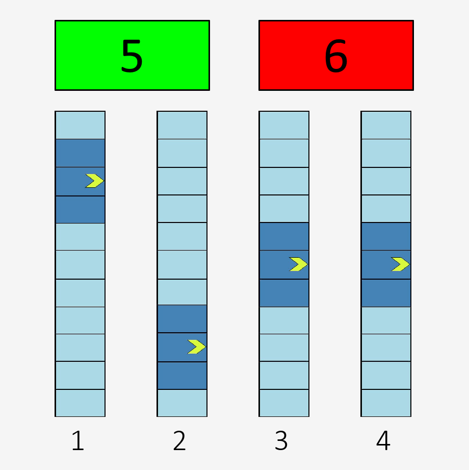
(b) System Monitoring

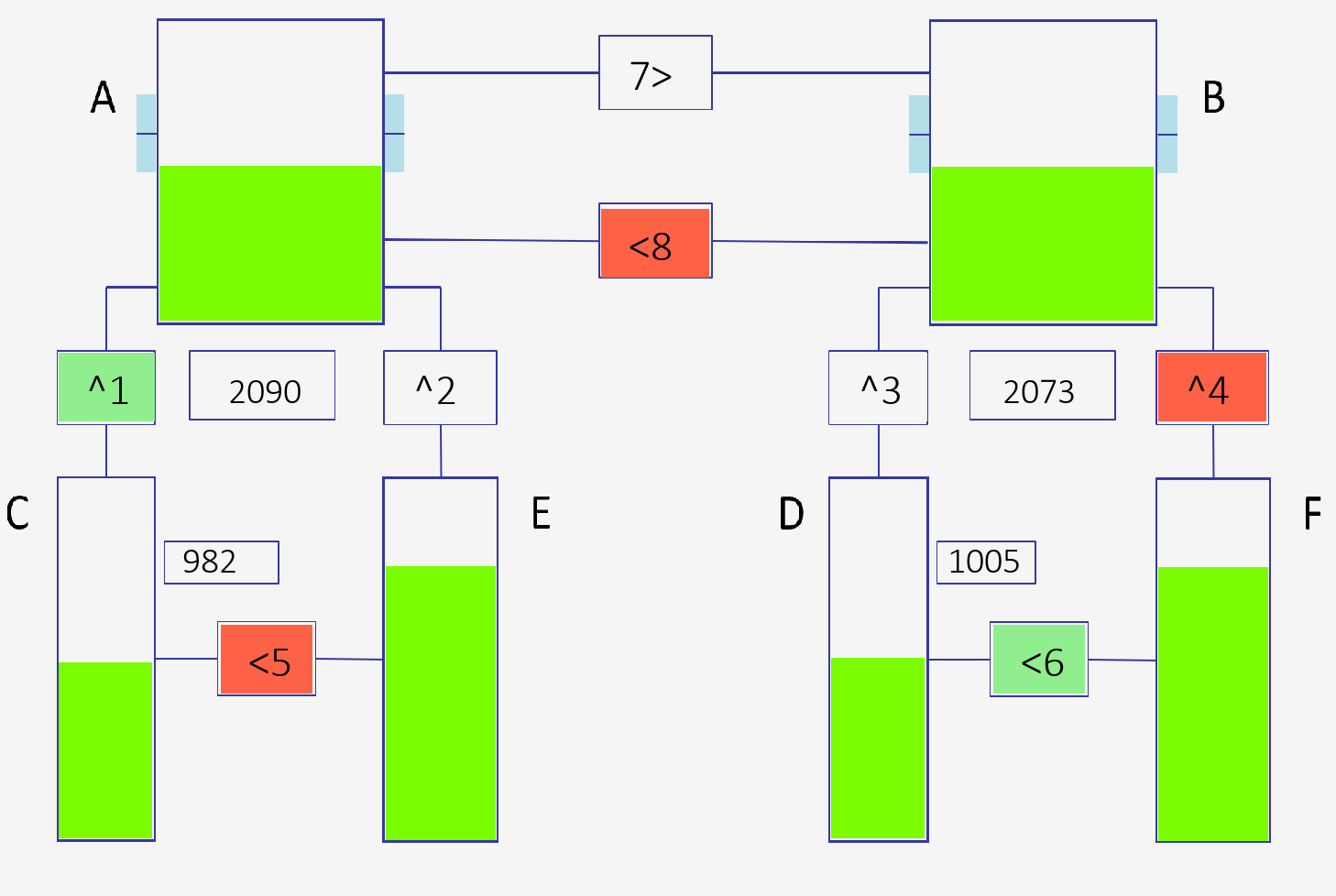
(c) Resource Management

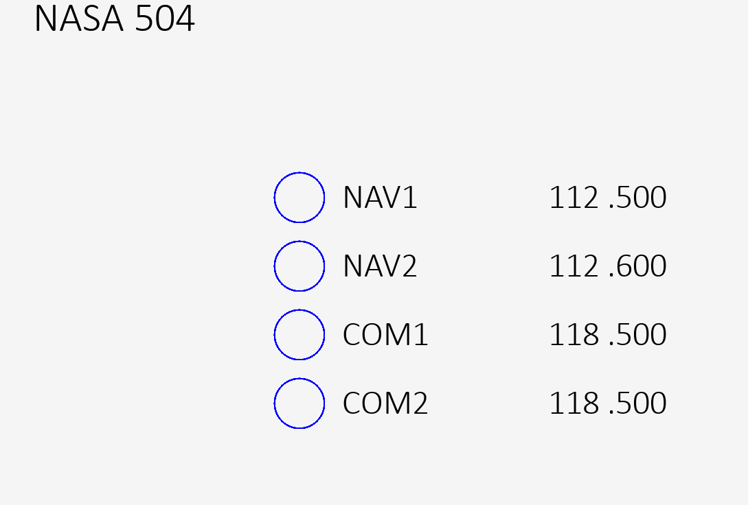
(d) Communications

Figure 1: The NASA MATB-II Tasks.

The tracking task, depicted in Fig. 1(a), required participants to keep the circle in the middle of the cross-hairs using a joystick. The system monitoring task, shown in Fig. 1(b), required monitoring two colored lights and four gauges. If the green or the red light turned on, an out of range value required resetting. The four gauge indicators randomly moved up and down, typically remaining in the middle. Resetting required pressing the corresponding number key on the keyboard. The resource management task included six fuel tanks (A-F) and eight fuel pumps (1-8), shown in Fig. 1(c). The arrow by the fuel pump’s number indicated the fuel flow direction. Participants were to maintain the fuel levels of Tanks A and B by turning the fuel pumps on or off. Fuel Tanks C and D had finite fuel levels, while Tanks E and F had an infinite supply. A pump turned red when it was unable to pump fuel. The communications task required listening to air-traffic control requests for radio changes, ignoring requests not directed to the participant’s call sign. Participants changed the specified radio to the specified frequency by selecting the desired radio and using arrows to change the radio’s frequency, as depicted in Fig. 1(d), and provided a verbal response. Finally, participants walked around the tables to attend to the other tasks whenever they heard a ping sound. Participants were free to move between tasks at any time, but the ping enforced a mandatory transition.

Task timings and occurrences were chosen such that the correct workload condition, or task density, was elicited. The IMPRINT Pro human performance modeling tool was used to model the tasks for each workload level and ordering prior to conducting the evaluation and provided anchors for selecting a task’s correct workload value [15], as well as to provide continuous workload values to act as pseudo ground truth labels for all workload machine learning models.

2.1 Prediction Model Design and Validation

Two direct time series forecasting methods were evaluated, with historical workload estimates provided via pretrained workload estimation models [16, 17, 18]. The univariate approach used only the overall historical workload estimates, or that of a single workload component, to predict the same component’s future workload. The multivariate approach used all seven components’ estimated workload to predict future workload. Both approaches used autoregressive feed forward neural networks with a “global" dataset of similar time series (i.e., other humans executing the mission plan) [19], and a leave-one-subject-out five-fold blocked cross validation method [20]. Models were trained with data from each participant with sufficient data to use the blocked cross validation (e.g., $>$ 30 min for 120 second (s) predictions using 240s lag horizons). Each four-layer neural network was implemented using PyTorch with two hidden layers of 128 nodes each. Models were trained using the Atom optimizer with a learning rate of 0.0001, a 128 batch size, and used early stopping to avoid overfitting. The models employed a 5s step size using prediction horizons of 60s, 120s, and 240s, and lag horizons of 30s, 60s, 120s and 240s. The prediction horizons and lag horizons were chosen to evaluate the maximum range afforded by the five folds (i.e., 600s).

3 Results and Discussion

Spearman correlations provide analysis of the similarity between the univariate or multivariate predictions and IMPRINT Pro, and were used to evaluate the models’ performance. Prior work established correlation values of $>0.7$ are considered high correlation, 0.5-0.69 are moderate, whereas correlation values below 0.5 are low, with values $<0.3$ regarded as negligible [21]. Moderate correlation values are deemed acceptable for prediction, with high correlation values preferred. Cognitive, visual, auditory and overall workload predictions are presented using both univariate and multivariate methods, alongside minimum and maximum lag horizon analysis. The remaining workload components are excluded due to insufficient lag horizon differences, or low correlation values.

3.1 Univariate Workload Prediction

Table 2: The univariate cognitive, visual, auditory and overall workload prediction Spearman correlations [mean (std)] by prediction and lag horizon.

Cognitive
	30s Lag	60s Lag	120s Lag	240s Lag
60s Pred.	0.48 (0.14)	0.52 (0.15)	0.56 (0.14)	0.64 (0.12)
120s Pred.	0.40 (0.13)	0.41 (0.13)	0.44 (0.13)	0.54 (0.13)
240s Pred.	0.25 (0.08)	0.25 (0.09)	0.31 (0.08)	0.57 (0.19)
Visual
60s Pred.	0.46 (0.13)	0.48 (0.13)	0.49 (0.13)	0.63 (0.11)
120s Pred.	0.35 (0.11)	0.37 (0.11)	0.39 (0.11)	0.54 (0.11)
240s Pred.	0.25 (0.11)	0.25 (0.11)	0.27 (0.09)	0.57 (0.16)
Auditory
60s Pred.	0.35 (0.12)	0.48 (0.18)	0.57 (0.21)	0.63 (0.13)
120s Pred.	0.41 (0.15)	0.46 (0.15)	0.53 (0.18)	0.59 (0.12)
240s Pred.	0.29 (0.09)	0.32 (0.09)	0.41 (0.11)	0.57 (0.13)
Overall
60s Pred.	0.56 (0.12)	0.57 (0.13)	0.59 (0.13)	0.68 (0.09)
120s Pred.	0.43 (0.13)	0.43 (0.13)	0.46 (0.13)	0.59 (0.09)
240s Pred.	0.21 (0.09)	0.23 (0.10)	0.26 (0.09)	0.57 (0.14)

The univariate cognitive, visual, auditory and overall workload predictions’ Spearman correlations increased as the lag horizon increased for each prediction horizon, as shown in Table 2. 60s overall workload prediction horizons required a minimum 30s lag horizon to attain an acceptable correlation, while the 120s and 240s prediction horizons required 240s lag horizons. The univariate overall workload prediction were significantly different between lag horizons per the Friedman test for the 60s (${\chi}^{2}(3,21)=39.17$, p $<$ 0.001, W = 0.49), 120s (${\chi}^{2}(3,20)=42.26$, p $<$ 0.001, W = 0.56) and 240s prediction horizons (${\chi}^{2}(3,20)=42.36$, p $<$ 0.001, W = 0.56). The Wilcoxon signed-ranked test indicated significant differences between 60s, 120s, and 240s lag horizons for the 60s prediction horizon (p $<$ 0.005, 0.64 $<$ Cohen’s d). Only the 120s and 240s lag horizons were significantly different for the 120s and 240s prediction horizons (p $<$ 0.001, 3.00 $<$ Cohen’s d).

The 60s univariate cognitive workload prediction horizons required a minimum 60s lag horizon for acceptable correlation and the 120s and 240s prediction horizons required 240s lag horizons. The cognitive workload prediction lag horizons differed significantly per the Friedman test for the 60s (${\chi}^{2}(3,37)=65.30$, p $<$ 0.001, W = 0.45), 120s (${\chi}^{2}(3,37)=51.26$, p $<$ 0.001, W = 0.36) and 240s prediction horizons (${\chi}^{2}(3,37)=63.26$, p $<$ 0.001, W = 0.44). The Wilcoxon signed-rank test indicated the univariate prediction Spearman correlations increased significantly with longer lag horizons for almost all prediction horizons, except the 30s and 60s lag horizons for the 240s prediction horizon (p $<$ 0.001, 0.86 $<$ Cohen’s d).

Each visual workload prediction horizon required 240s lag horizons to achieve acceptable correlation, with the Friedman test identifying significant differences between lag horizons for the 60s (${\chi}^{2}(3,37)=71.11$, p $<$ 0.001, W = 0.49), 120s (${\chi}^{2}(3,37)=76.23$, p $<$ 0.001, W = 0.53) and 240s (${\chi}^{2}(3,37)=52.75$, p $<$ 0.001, W = 0.37) prediction horizons. The Wilcoxon signed-rank test indicated significant univariate prediction Spearman correlation improvements as lag horizon increased for the 60s and 120s prediction horizons (p $<$ 0.005, 0.77 $<$ Cohen’s d). The only significant difference for the 240s prediction horizon was observed between the 120s and 240s lag horizons (p $<$ 0.001, 27.11 $<$ Cohen’s d).

Auditory workload’s 60s and 120s prediction horizons required a minimum 120s lag horizon for acceptable correlation. Acceptable results for the 240s prediction horizon required a 240s lag horizon. The Friedman test found significant differences for the univariate auditory workload predictions between lag horizons for the 60s (${\chi}^{2}(3,52)=118.96$, p $<$ 0.001, W = 0.58), 120s (${\chi}^{2}(3,52)=109.27$, p $<$ 0.001, W = 0.54), and 240s (${\chi}^{2}(3,52)=112.73$, p $<$ 0.001, W = 0.55) prediction horizons. The Wilcoxon signed-rank test showed significant univariate auditory workload prediction Spearman correlation differences between all lag horizons for all prediction horizons (p $<$ 0.001, 1.49 $<$ Cohen’s d).

Longer lag horizons improved the univariate workload predictions, but as the prediction horizon increased, these benefits decreased. Univariate workload predictions generally required 240s lag horizons to achieve acceptable results when predicting more than 60s into the future. This dependency suggests univariate workload predictions have difficulty making long-term workload predictions.

3.2 Multivariate Workload Prediction

Table 3: The multivariate cognitive, visual, auditory and overall workload prediction Spearman correlations [mean (std)] by prediction and lag horizon.

Cognitive
	30s Lag	60s Lag	120s Lag	240s Lag
60s Pred.	0.62 (0.08)	0.64 (0.07)	0.68 (0.09)	0.70 (0.10)
120s Pred.	0.51 (0.11)	0.55 (0.09)	0.56 (0.10)	0.53 (0.11)
240s Pred.	0.28 (0.11)	0.30 (0.11)	0.31 (0.12)	0.53 (0.21)
Visual
60s Pred.	0.61 (0.08)	0.63 (0.06)	0.64 (0.11)	0.71 (0.09)
120s Pred.	0.45 (0.08)	0.48 (0.07)	0.50 (0.11)	0.57 (0.09)
240s Pred.	0.29 (0.12)	0.28 (0.11)	0.33 (0.11)	0.62 (0.11)
Auditory
60s Pred.	0.55 (0.11)	0.60 (0.11)	0.63 (0.10)	0.67 (0.10)
120s Pred.	0.52 (0.05)	0.53 (0.07)	0.55 (0.07)	0.62 (0.09)
240s Pred.	0.35 (0.06)	0.37 (0.09)	0.41 (0.08)	0.54 (0.11)
Overall
60s Pred.	0.62 (0.08)	0.65 (0.07)	0.68 (0.10)	0.70 (0.05)
120s Pred.	0.51 (0.12)	0.55 (0.11)	0.57 (0.09)	0.58 (0.08)
240s Pred.	0.28 (0.12)	0.30 (0.12)	0.33 (0.13)	0.62 (0.12)

Spearman correlation values for multivariate predictions of overall, cognitive, auditory and visual workload increased as the lag horizon increased for each prediction horizon, as shown in Table 3. The 60s overall workload prediction horizons required a minimum 30s lag horizon for acceptable correlation, and a 240s lag horizon for high accuracy. Acceptable correlation values for the 120s and 240s prediction horizons required at least 30s and 240s lag horizons, respectively. Friedman tests indicated significant differences in overall workload predictions between lag horizons for 60s (${\chi}^{2}(3,21)=28.26$, p $<$ 0.001, W = 0.35), 120s (${\chi}^{2}(3,20)=25.68$, p $<$ 0.001, W = 0.34) and 240s prediction horizons (${\chi}^{2}(3,20)=36.90$, p $<$ 0.001, W = 0.49). The 60s and 120s prediction horizon correlations significantly increased between the 30s, 60s and 120s lag horizons (p $<$ 0.05, 1.89 $<$ Cohen’s d) per the Wilcoxon signed-rank test. The 240s prediction horizon correlations only significantly increased between the 120s and 240s (p $<$ 0.001, 1.87 $<$ Cohen’s d) lag horizons.

Cognitive workload’s 60s predictions required a 30s lag horizon for acceptable correlation, and a 240s lag horizon for high correlation. Acceptable results for 120s and 240s prediction horizons required 30s and 240s lag horizons, respectively. The Friedman test indicated the cognitive workload Spearman correlation significantly differed between lag horizons for the 60s (${\chi}^{2}(3,21)=27.91$, p $<$ 0.001, W = 0.35), and 240s (${\chi}^{2}(3,20)=23.82$, p $<$ 0.001, W = 0.31) prediction horizons. The Wilcoxon signed-rank test found significant Spearman correlation increases with increased lag horizons for the 30s, 60s and 120s lag horizons within the 60s prediction horizon (p $<$ 0.05, 2.04 $<$ Cohen’s d), and between the 120s and 240s lag horizons within the 240s prediction horizon (p $<$ 0.005, 15.54 $<$ Cohen’s d).

The 60s visual workload prediction horizons required a 30s lag horizon for acceptable correlation, and a 240s lag horizon for high correlation. The 120s and 240s prediction horizons required 120s and 240s lag horizons, respectively, to achieve acceptable results. The Friedman test for the visual multivariate prediction indicated significant differences between lag horizons for the 60s (${\chi}^{2}(3,21)=24.60$, p $<$ 0.001, W = 0.31), 120s (${\chi}^{2}(3,20)=22.26$, p $<$ 0.001, W = 0.29) and 240s (${\chi}^{2}(3,20)=41.58$, p $<$ 0.001, W = 0.55) prediction horizons. Wilcoxon signed-ranked tests showed significant increases in Spearman correlation as the lag horizon increased for the 30s, 60s and 120s horizons within the 60s and 120s prediction horizons based on the Wilcoxon signed-rank test (p $<$ 0.05, 5.17 $<$ Cohen’s d). Furthermore, the Spearman correlation significantly increased as the lag horizons increased for the 60s, 120s and 240s lag horizons within the 240s prediction horizon (p $<$ 0.001, 3.51 $<$ Cohen’s d).

Auditory workload prediction horizons of 60s and 120s required 30s lag horizons for acceptable correlation, whereas the 240s prediction horizon required a 240s lag horizon. The multivariate auditory workload prediction Friedman tests identified significant differences between lag horizons for the 60s (${\chi}^{2}(3,21)=35.57$, p $<$ 0.001, W = 0.44), 120s (${\chi}^{2}(3,20)=18.06$, p $<$ 0.001, W = 0.24), and 240s (${\chi}^{2}(3,20)=27.42$, p $<$ 0.001, W = 0.36) prediction horizons. The Wilcoxon signed-rank test indicated Spearman correlations increased significantly as the lag horizon increased in almost all cases (p $<$ 0.05, 0.79 $<$ Cohen’s d). The differences were not significant for 60s predictions between the 120s and 240s lag horizon, and between 60s and 120s lag horizons for the 120s prediction horizon.

Prediction horizons up to 120s had significantly improved accuracy with lag horizons up to 120s, after which out-of-date historical information resulted in diminishing returns. The 240s prediction horizon accuracy only significantly increased with a 240s lag horizon. These results suggest two paradigms for lag horizon selection. Shorter prediction horizons may have optimal lag horizons set by the workload value autocorrelation length. Alternatively, longer prediction horizons rely on points of high seasonality to select lag horizons.

4 Conclusion

Two direct time series forecasting approaches predicted future workload states using historical workload estimates. Lag horizons were investigated to determine how much data is required for each prediction horizon, and when further historical information ceased to improve predictions. These findings suggest univariate predictions required longer lag horizons. Conversely, multivariate predictions’ lag horizon may be set by the autocorrelation length or specific points of high seasonality. These workload prediction approaches using wearable sensors can better inform robot adaptation and may improve human-robot team performance in dynamic environments.

References

- [1] Y.-Y. Yeh and C. D. Wickens, “Dissociation of performance and subjective measures of workload,” Human Factors, vol. 30, no. 1, pp. 111–120, 1988.
- [2] C. D. Wickens, S. E. Gordon, Y. Liu, and J. Lee, An Introduction to Human Factors Engineering. Pearson Prentice Hall Upper Saddle River, NJ, 2004, vol. 2.
- [3] J. Heard and J. A. Adams, “Multi-dimensional human workload assessment for supervisory human–machine teams,” Journal of Cognitive Engineering and Decision Making, vol. 13, no. 3, pp. 146–170, 2019.
- [4] Y. Brand and A. Schulte, “Model-based prediction of workload for adaptive associate systems,” in IEEE International Conference on Systems, Man, and Cybernetics, 2017, pp. 1722–1727.
- [5] U. Boehm, D. Matzke, M. Gretton, S. Castro, J. Cooper, M. Skinner, D. Strayer, and A. Heathcote, “Real-time prediction of short-timescale fluctuations in cognitive workload,” Cognitive Research: Principles and Implications, vol. 6, no. 1, pp. 1–29, 2021.
- [6] Y. Pang, J. Hu, C. S. Lieber, N. J. Cooke, and Y. Liu, “Air traffic controller workload level prediction using conformalized dynamical graph learning,” Advanced Engineering Informatics, vol. 57, p. 102113, 2023.
- [7] W. Wei, X. Fu, Y. Zhu, N. Lu, and S. Ma, “Classification and prediction of driver’s mental workload based on long time sequences and multiple physiological factors,” IEEE Access, vol. 11, pp. 81 725–81 736, 2023.
- [8] Y. Qin and T. Bulbul, “Electroencephalogram-based mental workload prediction for using augmented reality head mounted display in construction assembly: A deep learning approach,” Automation in Construction, vol. 152, p. 104892, 2023.
- [9] N. Grimaldi, Y. Liu, R. McKendrick, J. Ruiz, and D. Kaber, “Deep learning forecast of cognitive workload using fnirs data,” in IEEE International Conference on Human-Machine Systems, 2024, pp. 1–6.
- [10] W. Yu, D. Jin, F. Zhao, and X. Zhang, “Towards pilot’s situation awareness enhancement: A framework of adaptive interaction system and its realization,” International Society of Automation Transactions, vol. 132, pp. 109–119, 2023.
- [11] R. J. Hyndman and G. Athanasopoulos, Forecasting: Principles and Practice. Melbourne, Australia: OTexts, 2018, ch. 3.
- [12] J. H. F. Flores, P. M. Engel, and R. C. Pinto, “Autocorrelation and partial autocorrelation functions to improve neural networks models on univariate time series forecasting,” in International Joint Conference on Neural Networks, 2012, pp. 1–8.
- [13] K. Kandananond, “A comparison of various forecasting methods for autocorrelated time series,” International Journal of Engineering Business Management, vol. 4, p. 4, 2012.
- [14] Y. Santiago-Espada, R. R. Myer, K. A. Latorella, and J. R. Comstock Jr, “The multi-attribute task battery II (MATB-II) software for human performance and workload research: A user’s guide,” NASA, Tech. Rep. NASA/TM–2011-217164, 2011.
- [15] D. K. Mitchell, “Mental workload and arl workload modeling tools,” Army Research Lab Aberdeen Proving Ground MD, Tech. Rep. ARL-TN-161, 2000.
- [16] J. Bhagat Smith, P. Baskaran, and J. A. Adams, “Decomposed physical workload estimation for human-robot teams,” in IEEE International Conference on Human-Machine Systems, 2022, pp. 1–6.
- [17] J. Bhagat Smith, S. A. Toribio, P. Baskaran, and J. A. Adams, “Uncertainty-aware visual workload estimation for human-robot teams,” in Conference on Cognitive and Computational Aspects of Situation Management, 2023.
- [18] J. R. Bhagat Smith, “Adaptive workload estimation for human-robot teams,” Ph.D. dissertation, Oregon State University, 2024.
- [19] K. P. Murphy, Probabilistic Machine Learning: Advanced Topics. MIT Press, 2023, ch. 29. [Online]. Available: http://probml.github.io/book2
- [20] V. Cerqueira, L. Torgo, and I. Mozetič, “Evaluating time series forecasting models: An empirical study on performance estimation methods,” Machine Learning, vol. 109, pp. 1997–2028, 2020.
- [21] D. E. Hinkle, W. Wiersma, and S. G. Jurs, Applied statistics for the behavioral sciences. Houghton Mifflin Boston, 2003, vol. 663.