Constant-Sum High-Order Barrier Functions
for Safety Between Parallel Boundaries
Abstract
This paper takes a step towards addressing the difficulty of constructing Control Barrier Functions (CBFs) for parallel safety boundaries. A single CBF for both boundaries has been reported to be difficult to validate for safety, and we identify why this challenge is inherent. To overcome this, the proposed method constructs separate CBFs for each boundary. We begin by presenting results for the relative degree one case and then extend these to higher relative degrees using the CBF backstepping technique, establishing conditions that guarantee safety. Finally, we showcase our method by applying it to a unicycle system, deriving a simple, verifiable condition to validate the target CBFs for direct implementation of our results.
I Introduction
Safety is a growing concern as autonomous technologies expand across various sectors, increasing interest in safety-critical control. Control Barrier Functions (CBFs) [1, 2] have gained popularity for their ability to enforce safety, with minimal deviation from nominal objectives when used with the quadratic program (QP) formulation [3, 4] leading to many findings [5, 6, 7]. However, implementing CBF-QP safety filters can be challenging, particularly for high and mixed relative degree CBFs, where absent control inputs in the first derivative of the safety constraint cannot give safety guarantees. To address this, several methods have been proposed, with High Order CBFs (HOCBFs) [8] being among the most widely used. Nevertheless, constructing such CBFs remains a nontrivial task.
We focus on the case where the objective is to keep the system within parallel boundaries. In this scenario, the construction of a valid CBF can be particularly challenging at the midway point between the boundaries, where the gradient of the safety constraint often vanishes. This leads to a loss of control authority, making safety enforcement difficult in any direction. Such issues were observed in Examples 2 and 5 of [9], where traditional single CBF approaches with high relative degree techniques failed to ensure safety. While methods such as [10] and [11] have been proposed, we take a different approach, drawing insights from [12] and [7], and generalize them into a more flexible and systematic framework.
In this paper, we show that utilizing two CBFs for parallel boundaries can provide advantages over using a single CBF. Although numerous studies have explored the use of multiple CBFs, such as [13] and [14], this work uses the control-sharing property as presented in [15]. However, the work in [15] assumes that the Lie derivative in the control direction is never zero. Our approach relaxes this assumption by explicitly verifying feasibility when the Lie derivative is zero, thereby accommodating potential sign changes of the Lie derivative. Furthermore, we extend the single-input result in [15] to multi-input systems when the safety boundary is parallel.
This formulation is extended to high relative degree CBFs by utilizing the CBF backstepping technique, having roots in [16] that predates the formulation of CBFs. Modern translations to CBFs can be found in [5, 7, 17]. While the target CBF transformations in this technique are similar to HOCBFs, the key difference is in the gain design. By choosing gains based on the system’s initial condition, the induced safe set guarantees the initial states are included, eliminating the need to retune parameters as in HOCBFs. Due to this useful property, the backstepping method has been applied to works such as simultaneous lane-keeping and obstacle avoidance [12], prescribed time safety filters (PTSf) [5], Stefan Model PDEs [7, 18], and unknown obstacle avoidance [17].
We note that the above CBF backstepping method differs from the backstepping approach defined in [10], which also addresses high relative degree problems but is inspired by traditional Lyapunov backstepping, where virtual controls transform a system into a target system. While both methods ask the same fundamental question, they differ significantly in the choice of the target system. For clarity, when we say CBF backstepping, we refer to the backstepping as in [16].
This work proposes a framework using two CBFs to enforce parallel safety boundaries, applicable to both relative degree one and arbitrarily high relative degree CBFs with the associated QP admitting a closed-form solution. A unicycle example illustrates the method’s effectiveness, including a sufficient condition for the target CBF’s validity.
II Preliminaries
We start with a preliminary overview of CBFs [1] outlining their definitions and key properties. Consider the following nonlinear control affine system:
| (1) |
with and unbounded input .
Definition 1
A scalar-valued continuously differentiable function with the property that and is defined as a Barrier Function (BF) candidate. The set is defined as the safe set, the set is the interior set, and the set is the boundary set.
Definition 2
A continuously differentiable function , is a Control Barrier Function (CBF) if there exists an extended class function such that for the control system (1):
| (2) |
Note that since the control input is assumed unbounded (i.e., ), condition (2) is equivalent to:
| (3) |
Lemma 1
We now introduce our motivational problem.
III Motivational Problem
The following problem was highlighted in [9] and [11]. Consider the double integrator system: , where . To enforce , we define the safe set as . A common CBF choice is , but since for all , it can be seen to have a relative degree of 2.
To address this, we use the CBF backstepping method to construct a target CBF , with the gain choice . The resulting CBF condition is where is the liveness gain for . We observe that at , the safety filter loses control authority (i.e., ). When , the CBF condition requires that , which does not hold for all and therefore cannot guarantee safety. Similar conditions arise when using HOCBFs as reported in [9] and [11].
This problem arises because the gradient vanishes at , where has a local maximum. Instead, we propose an alternative approach that decomposes the single CBF constraint into two, removing the loss of control authority due to the gradient vanishing while maintaining safety. Our method generalizes ideas from [12] and [7] in a more flexible framework.
IV Control Barrier Functions with Parallel Safety Boundaries
Consider two CBFs, and , for system (1), both having uniform relative degree , with corresponding safe sets and . The ideal safe set is then given by the intersection of these sets, i.e., . We introduce a class of CBFs in the form of the following definition, which makes this process streamlined.
Definition 3
A pair of candidate CBFs and is parallel if there exists a constant such that:
| (4) |
We note that the constant-sum expression in (4) is a special case of the convex combination with . However, since the scaling factors can be rescaled into the CBFs without affecting the safe set, we opt to study the constant-sum formulation to clearly illustrate its utility.
The parallel structure is particularly useful as it allows for a more systematic expression of the combined safety condition. A key property of the parallel CBFs is that , which represents two parallel safety boundaries with the combined safe set defined between them. We now demonstrate how this property can be used to derive a safety filter.
IV-A Relative Degree One
We first present the result for the case of relative degree one. Suppose and are parallel and both have a relative degree of . Taking the time derivative of and yields the CBF conditions:
| (5) | |||
| (6) |
where and are extended class functions. Since and are parallel, without loss of generality, (6) can be rewritten as and combining with (5), we arrive at the following joint constraint:
| (7) | ||||
| (8) | ||||
| (9) |
Then, to derive the control law, we introduce the quadratic program (QP)[3] formulation as follows:
| (10) | |||
| (11) |
First, we establish that the QP problem (10)–(11) is always feasible when and are valid CBFs and are parallel. A necessary and sufficient condition for ensuring feasibility in such cases is to show that and have the control-sharing property [15, Thm. 1]. That is, feasibility is guaranteed if the inequality holds for all . However, [15] assumes that and are never zero. This was a restrictive assumption that also limits the sign of the terms to be constant. To address cases where this assumption does not hold, we further show that . The following lemma formalizes this result.
Lemma 2
Proof:
Since and are CBFs, from (3), we have the following properties:
| (12) | ||||
| (13) |
Then, using the fact that and are parallel, we rewrite (13) as:
| (14) |
To prove the second part, we observe that . The trivial choice of where results in . Thus, there exist extended class functions and such that for all . ∎
With the feasibility established, we prove that the QP problem (10)–(11) has a closed-form solution.
Proof:
In the case where , we have shown in Lemma 2 that , regardless of the control input . Hence, the optimal solution to (10) is .
For the case , we must verify systematically. Noting that both the objective function and constraints are convex, the Karush-Kuhn-Tucker (KKT) conditions [21] provide necessary and sufficient conditions for to be the optimal solution. Namely, we must show that there exist such that
| (18) | |||
| (19) | |||
| (20) | |||
| (21) | |||
| (22) |
Here, (18) is referred to as the stationarity condition, (19) as the primal feasibility condition, (20) as the dual feasibility condition, and (21)–(22) as the complementary slackness condition.
Case 1: Suppose . Then, , as seen from (21)–(22) since neither constraint is active. From (18), we get , which matches the expression in (15).
Case 2: Suppose . Then, and from (18) we get the expression to get that from (21). Then, solving for :
| (23) |
From (20), since , it follows that if , then we must have . Substituting the expression for into the expression for again, we obtain
| (24) |
which matches with (15) when .
Case 3: Similar to case 2.
We summarize this result in Theorem 2.
Theorem 2
Proof:
Lemma 2 establishes the existence of extended class functions and such that the QP problem (10)–(11) is always feasible. Then, the closed-form solution given in Theorem 1 guarantees that and for all . If the initial conditions satisfy and , by Lemma 1, it follows that and for all . Hence, the set is forward invariant. ∎
IV-B High Relative Degree
Suppose and are parallel with relative degree . We apply the CBF backstepping technique, starting with the following necessary assumption.
Assumption 1
and are -times differentiable with and . That is, .
Now, we define , , and to proceed with the CBF backstepping algorithm. Taking the time derivative of and , and adding zero yields:
| (25) | ||||
| (26) | ||||
| (27) |
which gives:
| (28) | ||||
| (29) |
Then, from Assumption 1, we can choose the gains as:
| (30) |
to guarantee that . This also allows us to rewrite (29) as , where we define .
We now iterate this procedure until the target CBF transformation is acquired.
| (31) | ||||
| (32) | ||||
| (33) | ||||
| (34) |
for where and
| (35) |
which is strictly positive.
The induced safe set for the target CBF is then:
| (36) |
where and , with and , where .
It is important to note, while it may seem that the set does not include all , the gain choice in (35) adapts the sets and based on the initial condition . As a result, for all , the point is included in . This is a key difference from HOCBFs [8].
Then, we see that if the set is kept forward invariant, then by design and remain positive for all . However, it must be verified that and are valid CBFs at least in the set . That is, we must verify that
| (37) | ||||
| (38) |
where and are extended class functions, for all . Verifying their validity as CBFs is highly dependent on the system and constraints. Hence, we take it as the following assumption:
Assumption 2
and are valid CBFs for system (1) in the set .
We summarize this result in Theorem 3.
Theorem 3
For system (1), suppose and , with relative degree , are parallel and satisfy Assumption 1. Let (as in (33)–(34)) satisfy Assumption 2. Then, there exist extended class functions and such that applying (15) with , to (1) guarantees for all . Namely, the system remains safe under all nominal control inputs.
Proof:
Compared to recent works such as [10] and [11], our method offers advantages in both design flexibility and implementation. While [10] can be used to address the parallel boundary issue (as was shown in [9]), its safe set can be overly conservative due to parameter choices, which may require retuning to accommodate for certain initial conditions in the original safe set. In contrast, our method adaptively selects gains (35) based on the initial condition, ensuring it always lies within the induced safe set.
Relative to the Rectified CBF (ReCBF) approach in [11], our framework is simpler to implement, particularly for high relative degree CBFs. The work in [11] uses ReLU (or ) functions to rectify high relative degree CBFs, but because the QP safety filters require differentiating the CBF, the approach relies on carefully chosen hyperparameters to make the ReLU expressions continuously differentiable. This becomes increasingly delicate as the relative degree increases, since the ReLU expressions may need to be continuously differentiable up to times, where is the original CBF’s relative degree. Our method, by comparison, provides a more straightforward algorithm with tunable parameters that only need to satisfy the condition in (35).
V Examples and Simulations
V-A Returning to the Motivational Problem
We revisit the double integrator system , with the safe set . We define the CBFs and , corresponding to the safe sets and , whose intersection forms . Since , they are parallel. Using backstepping, we assume initially and choose:
| (39) |
V-B Unicycle Between Parallel Boundaries
Consider the kinematic unicycle system , where are the positional states, is the heading angle, is the forward velocity input, and is the angular velocity input.
Suppose we are given two parallel positional constraints represented by candidate CBFs and , with safe sets and . Since both depend only on and , they have a relative degree of 1 with respect to and 2 with respect to , resulting in a mixed relative degree problem.
To first address this, we add an integrator and assume control over the vehicle’s forward acceleration similar to that in [17]. That is,
| (40) |
This essentially modifies the unicycle model to a simplified bicycle model [22] and results in a uniform relative degree problem. We now proceed with the backstepping procedure with the assumption that .
Since and are parallel, without loss of generality, we compute the backstepping terms with respect to . By choosing the appropriate gains as in (35), we get the following target CBF through the backstepping procedure:
| (41) |
with a corresponding safe set as in (36). Then, defining and , the time derivative is:
| (42) |
where
| (43) | ||||
| (44) |
Intuitively, if , the control loses agency over safety () only when the heading angle is perpendicular to the gradient, i.e., parallel to the safety boundary. Similarly, loses agency () when the heading angle is parallel to the gradient, i.e., perpendicular to the boundary, or if . Thus, only if the heading is parallel to the boundary and , forming the basis of the following claim.
Theorem 4
Proof:
Suppose for all . To establish that and are CBFs in , it suffices to verify that implies and implies for all as in (37)–(38). Noting that and are orthogonal, equations and vanish simultaneously only when and
| (45) |
Under this condition, (42) evaluates to zero, implying and . Since and holds for all , and are valid CBFs on . ∎
As an example, consider the positional constraints
| (46) | ||||
| (47) |
These constraints are parallel since , and their gradients are nonzero as , satisfying the sufficient condition in Theorem 4.
We compare this to the single CBF , which defines the same safe set as the intersection of the two parallel constraints. However, when using the CBF backstepping (or HOCBF) method, this formulation loses control authority along the midline , where . On this line, the CBF becomes ill-defined, and its validity depends on the system’s forward velocity and heading angle.
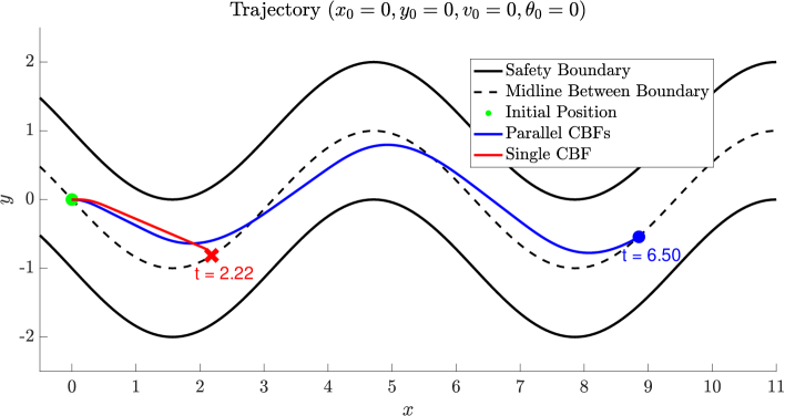
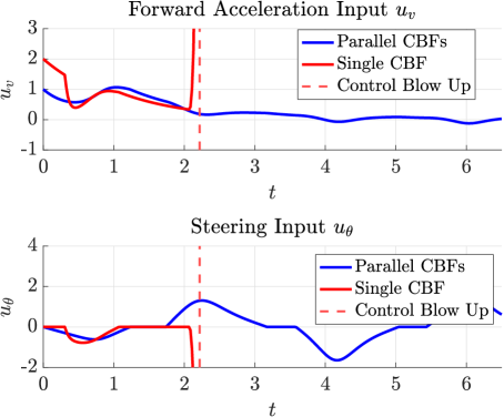
Figure 1 shows a simulation comparing both approaches. Both systems were initialized at the origin (i.e., ), which satisfies . All gain choices were set to (satisfying the backstepping design constraint), and all extended class functions were chosen as the identity function (i.e., ). The nominal control laws were and .
The single CBF-based safety filter (red) initially produced a valid trajectory, but as it re-encountered the midline, the vanishing gradient caused the CBF condition to fail, leading to a controller blow up at . In contrast, the parallel CBF-based safety filter (blue) remained well-defined, as the gradients never vanished in the safe set, and successfully kept the system safe with respect to the parallel boundaries.
VI Conclusion and Future Directions
In this paper, we addressed the challenge of valid CBFs for systems with parallel safety boundaries, a problem where relying on a single CBF is often invalid at the midway point between the boundaries. We identified that the core limitation arises from the vanishing gradient within the interior of the safe set and proposed an alternative approach that constructs separate CBFs for each boundary, effectively addressing the issue. This was validated through a simulation on a unicycle model.
Our method was based on unbounded control and CBFs with uniform relative degrees. While it does not directly address input constraints or mixed relative degree CBFs without modifications, extending the framework to handle such cases is a promising direction for future research. Broadening its applicability to unmodified systems like the unicycle is especially important in cases where structural modification is infeasible.
References
- [1] A. D. Ames, S. Coogan, M. Egerstedt, G. Notomista, K. Sreenath, and P. Tabuada, “Control barrier functions: Theory and applications,” in 2019 18th European control conference (ECC), pp. 3420–3431, Ieee, 2019.
- [2] P. Wieland and F. Allgöwer, “Constructive safety using control barrier functions,” IFAC Proceedings Volumes, vol. 40, no. 12, pp. 462–467, 2007.
- [3] A. D. Ames, J. W. Grizzle, and P. Tabuada, “Control barrier function based quadratic programs with application to adaptive cruise control,” in 53rd IEEE conference on decision and control, pp. 6271–6278, IEEE, 2014.
- [4] A. D. Ames, X. Xu, J. W. Grizzle, and P. Tabuada, “Control barrier function based quadratic programs for safety critical systems,” IEEE Transactions on Automatic Control, vol. 62, no. 8, pp. 3861–3876, 2017.
- [5] I. Abel, D. Steeves, M. Krstić, and M. Janković, “Prescribed-time safety design for strict-feedback nonlinear systems,” IEEE Transactions on Automatic Control, pp. 1–16, 2023.
- [6] T.-Y. Huang, S. Zhang, X. Dai, A. Capone, V. Todorovski, S. Sosnowski, and S. Hirche, “Learning-based prescribed-time safety for control of unknown systems with control barrier functions,” IEEE Control Systems Letters, vol. 8, pp. 1817–1822, 2024.
- [7] S. Koga and M. Krstic, “Safe PDE Backstepping QP Control With High Relative Degree CBFs: Stefan Model With Actuator Dynamics,” IEEE Transactions on Automatic Control, vol. 68, pp. 7195–7208, Dec. 2023.
- [8] W. Xiao and C. Belta, “High-order control barrier functions,” IEEE Transactions on Automatic Control, vol. 67, no. 7, pp. 3655–3662, 2021.
- [9] M. H. Cohen, T. G. Molnar, and A. D. Ames, “Safety-critical control for autonomous systems: Control barrier functions via reduced-order models,” Annual Reviews in Control, vol. 57, p. 100947, 2024.
- [10] A. J. Taylor, P. Ong, T. G. Molnar, and A. D. Ames, “Safe backstepping with control barrier functions,” in 2022 IEEE 61st Conference on Decision and Control (CDC), pp. 5775–5782, IEEE, 2022.
- [11] P. Ong, M. H. Cohen, T. G. Molnar, and A. D. Ames, “Rectified control barrier functions for high-order safety constraints,” IEEE Control Systems Letters, 2024.
- [12] S. Brüggemann, D. Steeves, and M. Krstic, “Simultaneous lane-keeping and obstacle avoidance by combining model predictive control and control barrier functions,” in 2022 IEEE 61st Conference on Decision and Control (CDC), pp. 5285–5290, IEEE, 2022.
- [13] T. G. Molnar and A. D. Ames, “Composing control barrier functions for complex safety specifications,” IEEE Control Systems Letters, vol. 7, pp. 3615–3620, 2023.
- [14] M. Alyaseen, N. Atanasov, and J. Cortes, “Safety-critical control of discontinuous systems with nonsmooth safe sets,” 2024.
- [15] X. Xu, “Constrained control of input–output linearizable systems using control sharing barrier functions,” Automatica, vol. 87, pp. 195–201, 2018.
- [16] M. Krstic and M. Bement, “Nonovershooting Control of Strict-Feedback Nonlinear Systems,” IEEE Transactions on Automatic Control, vol. 51, pp. 1938–1943, Dec. 2006.
- [17] K. H. Kim, M. Diagne, and M. Krstić, “Robust control barrier function design for high relative degree systems: Application to unknown moving obstacle collision avoidance,” 2024.
- [18] S. Koga, C. Demir, and M. Krstic, “Event-triggered safe stabilizing boundary control for the stefan pde system with actuator dynamics,” in 2023 American Control Conference (ACC), pp. 1794–1799, IEEE, 2023.
- [19] H. K. Khalil, Nonlinear systems. Upper Saddle River, N.J.: Prentice Hall, 2002.
- [20] P. Glotfelter, J. Cortés, and M. Egerstedt, “Nonsmooth barrier functions with applications to multi-robot systems,” IEEE control systems letters, vol. 1, no. 2, pp. 310–315, 2017.
- [21] S. Boyd and L. Vandenberghe, Convex optimization. Cambridge university press, 2004.
- [22] Y. Rahman, M. Jankovic, and M. Santillo, “Driver intent prediction with barrier functions,” in 2021 American Control Conference (ACC), pp. 224–230, IEEE, 2021.