Heuristic ansatz design for trainable ion-native digital-analog quantum circuits

Abstract

Variational quantum algorithms have become a standard approach for solving a wide range of problems on near-term quantum computers. Identifying an appropriate ansatz configuration for variational algorithms, however, remains a challenging task, especially when taking into account restrictions imposed by real quantum platforms. This motivated the development of digital-analog quantum circuits, where sequences of quantum gates are alternated with natural Hamiltonian evolutions. A prominent example is the use of the controllable long-range Ising interaction induced in ion-based quantum computers. This interaction has recently been applied to develop an algorithm similar to the quantum approximate optimization algorithm (QAOA), but native to the ion hardware. The performance of this algorithm has demonstrated a strong dependence on the strengths of the individual ion-ion interactions, which serve as ansatz hyperparameters. In this work, we propose a heuristic for identifying a problem-specific ansatz configuration, which enhances the trainability of the ion native digital-analog circuit. The proposed approach is systematically applied to random instances of the Sherrington-Kirkpatrick Hamiltonian for up to 15 qubits, providing favorable cost landscapes. As the result, the developed approach identifies a well-trainable ion native ansatz, which requires a lower circuit depth to solve specific problems as compared to standard QAOA. This brings the algorithm one step closer to its large scale practical implementation.

I Introduction

Current day quantum computers are inherently limited by both environmental and systematic noise. In the absence of error correction, these devices can only support the execution of short depth quantum circuits which fit within their coherence times [1, 2, 3, 4]. Within these restrictions, the variational model of quantum computing has been developed to explore the full potential of current hardware. In a variational quantum algorithm (VQA), a short depth parametrized quantum circuit is iteratively optimized by a classical co-processor in an attempt to minimize a given cost function [5]. This model has been proven to be universal [6] adapted for a wide variety of tasks, notably: the variational quantum eigensolvers (VQEs) [7, 8, 9, 10, 11, 12, 13, 14, 15] designed to approximate the ground energy of Hamiltonians, Hamiltonian simulations [16, 17, 18, 19], the quantum approximate optimization algorithm (QAOA) [20, 21, 22, 23, 24, 25, 26, 27, 28, 29, 30, 31, 32] designed to give approximate solutions to combinatorial optimization problems, quantum circuit compilers [33, 34, 35], machine learning [36, 37, 38, 39], among others [40, 41, 42, 43].

Despite the benefits offered by the variational model [44, 45, 46, 47, 48, 49], inaccurate results arising from gate imperfections and restricted circuit depth remain a prime concern [50, 51]. One pathway towards alleviating these limitations is the use of digital-analog quantum circuits which alternate between quantum gates and entangling natural Hamiltonian evolutions [52, 53, 54, 55], reducing the circuit dependence on entangling gates of limited fidelity. A typical example is the use of the long-range Ising interaction in trapped ion-based quantum computers [56, 57, 58, 59, 60, 61], which has been applied to quantum Hamiltonian simulations [62], QAOA compilation [49, 63] and used as an entangling layer in VQE circuits [64, 65]. In the same fashion, [66] has proposed to use this interaction as a substitute to the problem Hamiltonian exponent to generate a QAOA-like sequence capable of minimizing general $\mathbb{Z}_{2}$ symmetric combinatorial problems. The performance of this approach strongly depends on the choice of ion interactions referred to as ansatz hyperparameters. Indeed, problem agnostic hyperparameters can lead to trainability limitations induced by a large circuit expressivity [67] or by cost landscapes plagued with local minima [68]. On the other hand, as demonstrated in [66], certain problem-specific ion native ansatz hyperparameters can significantly improve the algorithmic performance, yet a procedure to identify them has been lacking so far.

Following the framework in [66], we develop an approach for identifying hyperparameters suitable for minimizing specific problem instances. For a QAOA-like ansatz we propose a heuristic based on optimizing a single layer circuit expectation value alternately over variational and circuit hyper- parameters using the block coordinate descent method (see, e.g., [69]). The proposed heuristic is benchmarked by performing Hamiltonian minimization for the Sherrington-Kirkpatrick (SK) model from $5$ to $15$ qubits with the coupling coefficients sampled from the standard normal distribution. This is a widely studied model in condensed matter physics, arising as a mean field approach to spin glasses [70, 71]. We demonstrate that the proposed heuristic identifies an ansatz structure, which provides a favorable optimization landscape. When compared to standard QAOA [20] and the previous approach proposed in [66], we establish that our heuristic ameliorates the optimization and notably reduces the circuit depth required to solve a problem.

The paper is structured as follows. Sec. II provides an outline of the ion native digital-analog circuit implementation based on the long-range Ising interactions. In Sec. III, we introduce a heuristic for searching problem-specific hyperparameters of the ion native ansatz that ameliorate the optimization in VQA. Sec. IV shows the numerical results, where we benchmark the proposed heuristic on random instances of the SK model and investigate how the choice of hyperparameters affects the ion-based QAOA performance. Sec. V summarizes and discusses the results.

II Ion native quantum ansatz

II.1 Global ion interaction

Trapped ion-based quantum computers are mostly known for their fully connected architecture, which allows executing entangling gates between any pair of ions in a trap [72, 73]. The interaction between ions is turned by the excitation of collective ion oscillation modes (i.e. phonons) at specific frequencies $\omega_{m}$ under laser radiation. If, however, the driving frequency is tuned far from the phonon frequencies (dispersive regime), the phonons are only virtually excited, inducing the evolution under the effective Hamiltonian [74, 58] (for details, see Appendix A),

$$H_{\mathrm{I}}=\sum_{i<j}J_{ij}X_{i}X_{j},$$ (1)

with $X_{j}$ being Pauli $X$ operator applied to the $j$-th qubit. The coupling coefficients in Eq. (1) are given by

$$J_{ij}=\Omega_{i}\Omega_{j}\sum_{m}\frac{\eta_{i}^{m}\eta_{j}^{m}\omega_{m}}{\mu^{2}-\omega_{m}^{2}}\equiv\Omega_{i}\Omega_{j}C_{ij}.$$ (2)

Here, the matrix $C_{ij}$ depends on the spectrum of phonon frequences $\omega_{m}$, Lamb-Dicke parameters $\eta_{j}^{m}$ which quantify the displacement of the $j$-th ion in the $m$-th phonon mode, and laser detuning $\mu$ from the carrier frequency. The matrix $C_{ij}$ thus can be precalculated and kept fixed (for details, see Appendix B). A characteristic feature of the interaction (2) is that it can be controlled in the experiment by varying the Rabi frequencies $\Omega_{i}$ induced by a laser field individually for each ion [58]. Introducing the parameters $A_{j}=\Omega_{j}/\Omega_{\max}$, where $\Omega_{\max}$ is the maximum allowed Rabi frequency in the experiment, the Ising coupling coefficients (2) can be rewritten as

$$J_{ij}=A_{i}A_{j}\Omega_{\max}^{2}C_{ij},$$ (3)

where the dimensionless hyperparameters $A_{j}\in[-1,1]$ control the strength of pairwise interactions. As such, the ion-ion interaction can be characterized by a vector of hyperparameters $\bm{A}=(A_{1},\ldots,A_{n})$.

II.2 Ion native quantum circuit

Utilizing global interactions in variational circuits is beneficial, as they can naturally entangle the system allowing to avoid the extensive use of entangling quantum logical gates. For the uniform choice of the frequencies $\Omega_{j}=\Omega$, when the couplings (2) are approximated as a power decay law $J_{ij}\propto 1/|i-j|^{a}$, the interaction (1) has been used as an entangling block in hardware efficient ansatzes and the QAOA circuit [49, 64, 65]. In [66] the effective Hamiltonian (1) with the non-uniform choice of $\Omega_{j}$ has been used to generate an ion native ansatz in the form of a QAOA-like sequence

$$\ket{\psi_{p}(\bm{\beta},\bm{\gamma})}=\prod_{k=1}^{p} \biggl{[}e^{-i\beta_{k}H_{x}}\mathrm{H}_{+}e^{-i\gamma_{k}H_{\mathrm{I}}}\mathrm{H}_{+}\biggr{]}\ket{+}^{\otimes n},$$ (4)

where $\mathrm{H}_{+}=(|+\rangle\langle 0|+|-\rangle\langle 1|)^{\otimes n}$ is the Hadamard gate applied to all the qubits, $H_{x}=\sum_{i}X_{i}$ is the mixer Hamiltonian, and $(\bm{\beta},\bm{\gamma})\in[0,\pi)^{p}\times[0,2\pi)^{p}$ are the variational parameters. Similar to the settings of standard QAOA, the ansatz (4) has been applied to solving combinatorial optimization problems [20, 25], where a classical cost function $C(z)$ is encoded into a corresponding problem Hamiltonian

$$H_{P} =\sum_{z\in\{0,1\}^{n}}C(z)\outerproduct{z}{z},$$ (5)

following the energy minimization

$$E_{p}(\bm{\beta},\bm{\gamma}) =\bra{\psi_{p}(\bm{\beta},\bm{\gamma})}H_{\mathrm{P}}\ket{\psi_{p}(\bm{\beta},\bm{\gamma})}\to\min_{\bm{\beta},\bm{\gamma}}.$$ (6)

Approaching this problem in the standard QAOA setting would require implementation of the exponent $e^{-i\gamma H_{P}}$. In practice, this exponent has to be decomposed into a sequence of entangling gates of limited fidelity. Moreover, it can even require more layers to reach the same tolerance as compared to the ion native realization [66]. The ansatz (4) has also found application as a Hamiltonian variational ansatz [75, 76] in VQE [49]. In more general settings the layer of correlated single qubit rotations $e^{-i\beta H_{x}}$ can be substituted by a layer of arbitrary $SU(2)$ elements, making the ansatz universal [64].

Importantly, it has been shown that a problem-specific choice of the hyperparameters $\bm{A}$ can drastically improve the result of Hamiltonian minimization [66]. Indeed, as it is shown below, randomly generated non-symmetric hyperparameters $\bm{A}$ produce ansatzes of high expressivity. Potentially, they can solve arbitrary instances, but suffer from trainability limitations: even if a solution exists in the variational state space, it might be hard to locate [67, 68]. On the other hand, by adjusting hyperparameters $\bm{A}$ for each specific problem one can identify a well-trainable ansatz configuration, which also reduces the circuit depth required to find a solution. The latter is crucial for near-term quantum devices. In this paper, we focus on how to enhance the trainability of ansatz (4) by adjusting its hyperparameters $\bm{A}$.

III Heuristic for searching problem-specific hyperparameters

When searching for problem-specific trainable ansatz configurations, we observed that certain hyperparameters generate well-trainable circuits for a wide range of depths. In other words, well-trainable ansatz configurations found at a small circuit depths can preserve this property when used in deeper circuits. Based on this observation, we propose to search for ansatz hyperparameters by optimizing the energy for a single layer:

$$E(\bm{\theta},\bm{A})=\langle\psi_{1}(\bm{\theta};\bm{A})|H_{\mathrm{P}}|\psi_{1}(\bm{\theta};\bm{A})\rangle\to\min_{\begin{subarray}{c}\bm{\theta}\in\Theta\\ \bm{A}\in[-1,1]^{\times n}\end{subarray}}.$$ (7)

We found that hyperparameters optimized in this fashion provide a trainable cost landscape with respect to variational parameters for a single-layered ansatz — a property that is preserved for larger circuit depths, as we demonstrate in the next section.

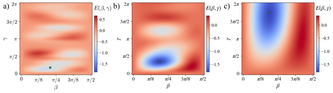
Figure 1: Typical cost landscape for the energy (7) of a single-layered ion native ansatz as a function of variational parameters $(\beta,\gamma)\in\Theta$ calculated using different configurations of hyperparameters: a) asymmetric ($A_{i}=1$, $\forall i\neq 1$; $A_{1}=-0.3$), b) $\bm{A}^{*}$ trained by our heuristic and c) $\alpha\bm{A}^{*}$ rescaled by the factor $\alpha=0.44$ after training. Green points depict the global minima.

A formal description of the proposed heuristic is given in Algorithm 1. The inputs are: the number of qubits $n$, the problem Hamiltonian $H_{\rm P}$, the maximal Rabi frequency $\Omega_{\max}$, the matrix $C_{ij}$ of the phonon contribution to the Ising couplings (3), the maximum allowed BCD iterations $k_{\max}$ and random restarts $m_{\max}$, the tolerance $\varepsilon$ for the convergence criteria, and the tolerance $\delta$ for detecting stagnation in a local minimum. For minimizing the energy (7), we use the block coordinate descent (BCD). This method alternately optimizes the cost function with respect to each block of variables $\bm{\theta}$ and $\bm{A}$. One of the main advantages of BCD is that it allows to optimize each block of variables by methods, which take into account specific properties of the problem (see, e.g., [69]). The algorithm starts by sampling a random initial guess for hyperparameters $\bm{A}_{0}$ uniformly distributed on $[-1,1]^{n}$. Then, it proceeds to the main BCD iterations loop, where the energy (7) is minimized alternately over $\bm{\theta}$ and $\bm{A}$.

On each iteration $k$ of the BCD loop, the current approximation $\bm{A}_{k}$ for hyperparameters is fixed and the energy $E(\bm{\theta},\bm{A}_{k})$ is minimized over a pair of variational parameters $\bm{\theta}=(\beta,\gamma)\in\Theta$ (for details, see Appendix C). Once this step is complete, the BCD convergence criteria

$$E_{k}<\varepsilon,$$ (8)

is checked. Here, $E_{k}=\min_{\bm{\theta}\in\Theta}E(\bm{\theta},\bm{A}_{k})$ is the optimized energy on the $k$-th iteration. If the criteria (8) is met, the algorithm terminates and returns $\bm{A}_{k}$ as the optimal ansatz configuration $\bm{A}^{*}$. Note that the tolerance $\varepsilon$ in Eq. (8) is chosen empirically. For the combinatorial optimization problems considered later, encoded into traceless Hamiltonians, $\varepsilon$ was set to $0.5\lambda_{0}$. In these settings the criteria (8) requires a prior knowledge of the ground state energy $\lambda_{0}$, which is typically not accessible in real experiments. In this case, one should either introduce a new empirical convergence criteria or run the algorithm multiple times to choose the best ansatz configuration.

Algorithm 1 Heuristic for searching a well-trainable hyperparameters configuration of the ion native ansatz (4) for a specific problem Hamiltonian $H_{\rm P}$.

1:$n$, $H_{\rm P}$, $\Omega_{\max}$, $C_{ij}$, $k_{\max}$, $m_{\max}$, $\varepsilon$, $\delta$

2:$\bm{A}^{*}$

3:$L\leftarrow[\,\,]$ // Empty list to store energies and $\bm{A}$s

4:for $m$ = 1 to $m_{max}$ do

5:  Sample random guess: $\bm{A}_{1}\sim\mathcal{U}(-1,1)^{n}$

6:  $E_{-1}$ = $\infty$ // or a large enough number

7:  for $k$ = 1 to $k_{max}$ do

8:   $\bm{\theta}_{k}\leftarrow\operatorname*{arg\,min}_{\bm{\theta}\in\Theta}E(\bm{\theta},\bm{A}_{k})$

9:   $E_{k}\leftarrow E(\bm{\theta}_{k},\bm{A}_{k})$

10:   if $E_{k}<\varepsilon$ then // Check convergence

11:     return $\bm{A}_{k}$

12:   end if

13:   if $|E_{k}-E_{-1}|<\delta$ then // Check stagnation

14:     break

15:   end if

16:   $\bm{A}_{k+1}\leftarrow~\operatorname*{arg\,min}_{\bm{A}\in[-1,1]^{n}}E(\bm{\theta}_{k},\bm{A})$

17:   $E_{-1}\leftarrow E_{k}$

18:  end for

19:  append $[E_{k},\bm{A}_{k}]$ to $L$

20:end for

21:return $\bm{A}$ with the smallest energy from $L$

If the optimization exceeds the maximum allowed number of iterations $k_{\max}$ or gets stuck in a local minimum without significant improvement, it restarts with a new initial guess $\bm{A}_{0}$ for hyperparameters, while the iteration counter $k$ is reset to zero. Otherwise, the energy $E(\bm{\theta}_{k},\bm{A})$ is minimized over the vector $\bm{A}$ of $n$ hyperparameters, with $\bm{A}_{k}$ taken as an initial guess. During this process, the block of variational parameters is kept fixed at $\bm{\theta}=\bm{\theta}_{k}$. After this step, the next approximation to the optimal configuration of hyperparameters, $\bm{A}_{k+1}=\operatorname*{arg\,min}_{\bm{A}\in[-1,1]^{n}}E(\bm{\theta}_{k},\bm{A})$ is obtained, and the iterations counter $k$ is increased by $1$.

The heuristic continues the BCD iterations, alternately optimizing (7) with respect to $\bm{\theta}$ and $\bm{A}$ until either the criteria (8) is met or the number of random restarts exceeds $m_{\max}$. If the latter occurs, the method returns the hyperparameters that provided the smallest energy (7) over all restarts. In practice, only a few iterations were required to reach the desired accuracy in (8) for the problem instances, considered in the next section.

At Fig. 1, we examine the effect of ansatz hyperparameters $\bm{A}^{*}$ trained by our heuristic on a typical single layer cost landscape $E(\beta,\gamma,\bm{A})$ with respect to variational parameters $(\beta,\gamma)\in\Theta$. For comparison, at Fig. 1a we show the landscape (7) provided by the asymmetric configuration $\bm{A}$, where $A_{i}=1$, $\forall i\neq i^{\prime}$ and $A_{i^{\prime}}$ detuned randomly (we set $A_{1}=-0.3$) as proposed in [66]. From Fig. 1a, we see that the cost landscape is highly non-convex plagued by multiple local minima. This is a serious limitation for the trainability of variational quantum algorithms [68], which only worsens upon increase of the circuit depth  [77]. In contrast, the configuration $\bm{A}^{*}$ trained by the proposed heuristic provides a more favorable optimization landscape with a single pronounced global minimum (see Fig. 1b), which is about 2.7 times deeper as compared to the one shown at Fig. 1a.

Note that the global minimum near $(\pi/6,\pi/3)$ in Fig. 1b is located inside a narrow gorge. This can limit the ansatz trainability, as the fraction of the parameter space below a certain cost function value becomes exponentially suppressed as $p$ increases [78, 79]. The gorge, however, can be widened by restricting the range of $\gamma$ to the vicinity of the global minimum. If the minimum is located in the region of small $\gamma$, this can effectively be realized by rescaling $\bm{A}$ by a factor $0<\alpha<1$ as

$$E(\beta,\gamma,\alpha\bm{A})=E(\beta,\alpha^{2}\gamma,\bm{A}).$$ (9)

As a result, the narrow gorge widens as shown at Fig. 1c, while the energy (7) starts to behave almost like a convex function. In order to find the optimal scaling factor $\alpha^{*}$, we construct a cost function $f(\alpha)$ that estimates the fraction of the parameter space $\Theta$ that corresponds to energy (7) bellow a certain value (for details, see Appendix C). This cost function is maximized to find $\alpha^{*}=\operatorname*{arg\,max}_{\alpha}f(\alpha)$.

Thus, the approach for searching problem-specific hyperparameters of the ion native ansatz (4) consists of two stages. First, the algorithm alternately minimizes the energy (7) over the variational and hyper- parameters to find the configuration $\bm{A}^{*}$ that provides a favorable optimization landscape. Second, the optimal scaling factor $\alpha^{*}$ for $\bm{A}^{*}$ is found to stretch the desired part of the cost landscape. This is achieved by maximizing the fraction of parameter space $\Theta$ below a certain energy threshold. As a result, the heuristic identifies the configuration $\alpha^{*}\bm{A}^{*}$ that allows to significantly improve the circuit trainability for $p>1$ layers, as demonstrated in the next section.

Note that the proposed method requires evaluating the energy only for a single layer ($p=1$) ansatz, which is efficient in terms of computational time and is accessible in the experiment. However, the bottleneck of this heuristic is the optimization of the cost (7) over $\bm{A}$ on each BCD iteration. The cost function (7) with respect to $\bm{A}$ is $n$-dimensional, while the shape of the optimization landscape is unknown. As $n$ increases, this step of the heuristic can become more challenging for standard optimization techniques.

IV Numerical results

IV.1 The problem

We test the proposed heuristic for the ion native QAOA, i.e. by solving combinatorial optimization problems with ansatz (4). As a testbed, we consider random instances of the Sherrington-Kirkpatrick (SK) Hamiltonian [70],

$$H_{\rm P}=\frac{1}{\sqrt{n}}\sum_{i<j}K_{ij}Z_{i}Z_{j},$$ (10)

where the all-to-all coupling coefficients $K_{ij}$ are sampled independently from a normal distribution with zero mean and unit variance. A detailed study of the performance of the standard QAOA applied for optimizing the SK model (10) can be found in [80]. We have additionally studied the performance of the proposed method for MAX-CUT on random and regular graphs, but no significant difference between the two models has been observed, so the rest of the work focuses on the SK model.

The simulations are performed for system sizes from $n=5$ to $15$ qubits. At each problem size $n$, the matrix $C_{ij}$ of phonon contribution to the Ising couplings (3) in the ion Hamiltonian $H_{\rm I}$ is calculated (for details, see Appendix B). For each random instance of (10), the proposed heuristic is applied to identify appropriate problem-specific hyperparameters of the ion native ansatz (4). The obtained ansatz configuration is then fixed and the energy (6) is minimized at different circuit depths $p$ using the layerwise training heuristic proposed in [51]. Note that in order to eliminate degeneracies in the parameter space $\Theta$ due to the $\mathbb{Z}_{2}$ symmetry, we restrict $\beta_{k}\in[0,\pi/2)$ in the simulations (see, e.g., [27]).

The performance of the algorithm is evaluated using two different metrics. The first metric is the normalized approximation ratio (see, e.g., [49]),

$$r=\frac{\lambda_{\max}-E_{p}(\bm{\beta}^{*},\bm{\gamma}^{*})}{\lambda_{\max}-\lambda_{0}},$$ (11)

where $\lambda_{\max}$ is the energy of the highest excited state of $H_{\rm P}$, and $(\bm{\beta}^{*},\bm{\gamma}^{*})$ are the optimal variational parameters obtained by optimizing the energy (6). The second one is the overlap $g(\psi)$ of a state $\ket{\psi}\equiv\ket{\psi_{p}(\bm{\beta}^{*},\bm{\gamma}^{*})}$ with the $d$-degenerate ground space of $H_{\rm P}$ (see, e.g., [51]),

$$g(\psi)=\sum_{j=1}^{d}|\bra{\phi_{j}}\ket{\psi}|^{2},$$ (12)

where $\ket{\phi_{j}}$ are the corresponding eigen basis states. We consider a simulation run to be successful, if the resulting overlap (12) surpasses the threshold $g(\psi)>0.5$. Note that a high approximation ratio does not necessarily guarantee a certain overlap with the ground state. According to the stability lemma [6], the relation between the two strongly depends on the spectral gap $\Delta$, which can be small for specific problem Hamiltonians $H_{\rm P}$.

IV.2 Effect of hyperparameters on ansatz trainability

We begin by demonstrating the role of an appropriate problem-specific choice of hyperparameters $\bm{A}$ on the trainability of the ion native circuit. For a randomly generated SK instance (see the inset at Fig. 2a), we compare the QAOA performance for two different configurations of $\bm{A}$. The first is the asymmetric one, where $A_{i}=1$, $\forall i\neq i^{\prime}$ and $A_{i^{\prime}}$ detuned randomly (we set $A_{1}=-0.3$). This configuration is known to be able to minimize all instances of the simplified model (10) with $K_{ij}=\pm 1$ for $n=6$ qubits using the QAOA circuit depth of up to $p=20$ layers [66]. The second one is a problem-specific configuration obtained from the proposed heuristic. The respective cost landscapes (7) for a single-layered ansatz are presented at Figs. 1a and 1c.

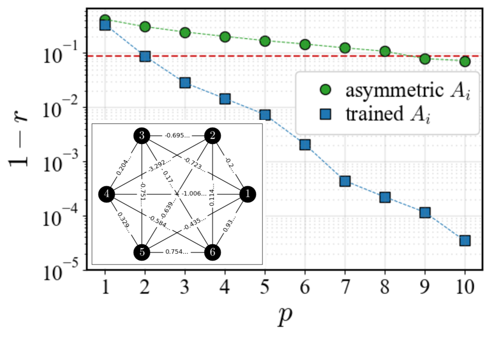
Figure 2: Performance of the ion native QAOA in terms of the fractional error $1-r$ as a function of the circuit depth $p$. The results are obtained for (i) the asymmetric configuration ($A_{i}=1$, $\forall i\neq 1$; $A_{1}=-0.3$), shown in green, and (ii) found by the heuristic, shown in blue. Red dashed line depicts the threshold, which guarantees the ground state overlap $g(\psi)=0.5$ from the stability lemma [6]. The inset depicts the coefficients $K_{ij}$ for the considered SK problem instance (10).

Fig. 2 shows the optimization results for the considered hyperparameter configurations at different circuit depths. Comparing the fractional error $1-r$ in these configurations, one can observe a dramatic difference in the algorithmic performance. For the asymmetric configuration of $\bm{A}$, the fractional error $1-r$ slowly decreases with $p$ reaching the threshold $g(\psi)>0.5$ at $p=9$ layers. In comparison, the problem-specific configuration of $\bm{A}$ obtained by the proposed heuristic drastically improves the performance of ion native QAOA. Here, the fractional error $1-r$ rapidly decreases with $p$ to about $10^{-5}$ at $p=10$. Moreover, in this case already $p=2$ layers of the QAOA circuit are sufficient to reach the threshold $g(\psi)>0.5$. Evidently, using appropriate problem-specific hyperparameters, one can drastically reduce the circuit depth required to reach a desired accuracy.

IV.3 Interplay between trainability and expressibility

The expressibility of a parameterized quantum circuit is defined by how uniformly it explores the unitary space [81]. Recent studies demonstrate that increasing the expressibility of an ansatz can result in smaller gradients of a cost function, which limits trainability [67]. However, for some specific quantum circuits such as the alternating layered ansatz the expressibility and trainability can coexist [82]. Here, we investigate the interplay between the expressive power and trainability for the ion native ansatz.

The expressibility is evaluated using a descriptor based on the Kullback-Leibler (KL) divergence [81],

$$D_{\rm KL}=\int_{0}^{1}\rho_{F}(x)\,\log{\frac{\rho_{F}(x)}{\rho_{\mathrm{Haar}}(x)}}\,{\mathrm{d}}x,$$ (13)

between the probability density function $\rho_{F}(x)$ for the distribution of fidelities $F=\bigl{|}\bra{\psi(\bm{\theta}_{1})}\ket{\psi(\bm{\theta}_{2})}\bigr{|}^{2}$ sampled uniformly from the ansatz, and for Haar random states

$$\rho_{\mathrm{Haar}}(x)=(N-1)(1-x)^{N-2}.$$ (14)

In Eq. (14), $N$ is the dimension of the Hilbert space of quantum states. The ansatz with smaller value of $D_{\rm KL}$ has a higher expressibility. The KL divergence (13) is evaluated in a range of ansatz circuit depths $p$. At each depth $p$, $10^{5}$ fidelities are produced from the ion native ansatz (4) by sampling variational parameters $(\bm{\beta},\bm{\gamma})$ uniformly from $\Theta$. For the Haar density (14) $N=2^{n-1}$ is used to account for the $\mathbb{Z}_{2}$ symmetry of the QAOA prepared states, $X^{\otimes n}\ket{\psi}=\ket{\psi}$.

Fig. 3 illustrates expressibility of the ion native ansatz (4) for $n=6$ qubits for the asymmetric and trained configurations of $\bm{A}$ from Sec. IV.2. Note that the descriptor (13) does not depend on a specific problem instance. From Fig. 3, we observe that the KL divergence for the asymmetric configuration rapidly decreases with $p$ to about $D_{\rm KL}\sim 10^{-4}$ and saturates starting from $p=6$ layers. For the trained hyperparameters, on the other hand, the ansatz expressibility is strongly limited: the KL divergence takes typical values $D_{\rm KL}\gtrsim 1$ and slowly decreases with $p$. This clearly demonstrates a higher expressive power of the asymmetric problem-agnostic configuration, compared to the problem-specific one. Thus, we observe the interplay between the trainability and expressibility of the ion native ansatz (4). By training hyperparameters we identify a problem-specific ansatz, designed to prepare a fraction of the Hilbert space, containing the solution. This can partially be attributed to the rescaling part of the heuristic, which decreases magnitudes of $\bm{A}$, effectively reducing the accessible phases of $\bm{\gamma}$, as per (9). This naturally limits the expressibility of the designed ansatz, locking it to the space in the vicinity of the solution, but allows to significantly enhance its trainability.

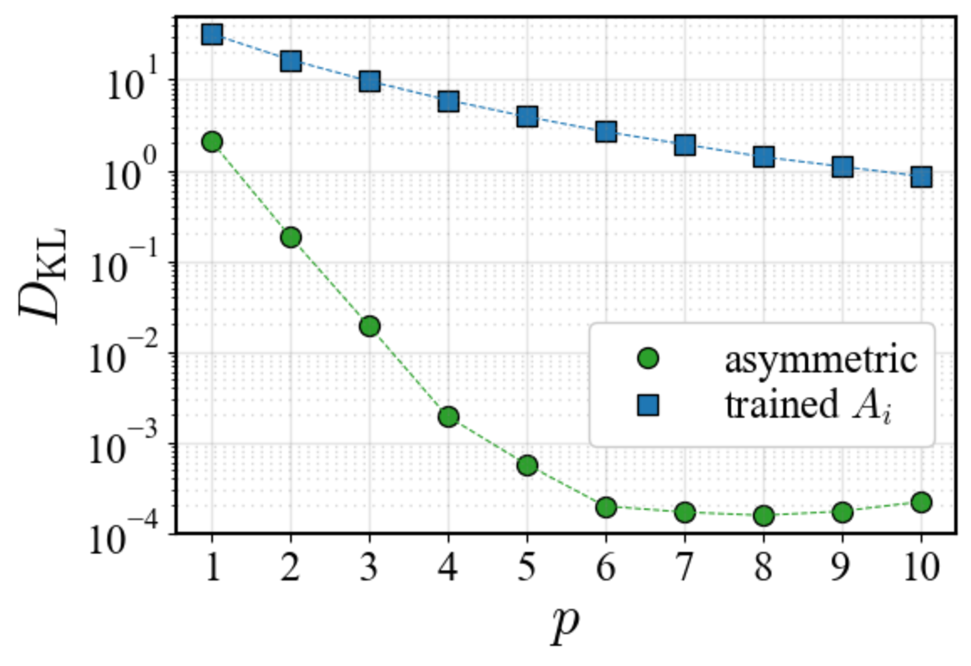
Figure 3: KL divergence (13) as a function of the circuit depth $p$ for the ion native ansatz (4) for $n=6$ qubits. The results are obtained for (i) the asymmetric configuration ($A_{i}=1$, $\forall i\neq 1$; $A_{1}=-0.3$), shown in green, and (ii) found by the heuristic, shown in blue. The considered SK instance is shown in the inset of Fig. 2a. Note that lower values of $D_{\rm KL}$ correspond to a more expressible circuit.

IV.4 Statistical evaluation on random instances

In this section we systematically investigate the performance of the proposed heuristic on random instances of the SK model (10) in the range from 5 to 10 qubits. As we show in Appendix D, for all problems of a given size, the required ground state overlap $g(\psi)>0.5$ can be achieved using the same circuit depth. This fact is demonstrated by solving the state preparation problem, where $p=2$ layers of the ion native ansatz (4) are sufficient to reach the desired overlap threshold for $n=5$–$10$. This, however, clearly ignores how hard it is to train such circuits and adjust hyperparameters when considering the Hamiltonian minimization. Thus, the solution at depth $p=2$, while exists, might be practically unattainable, therefore we relax it by considering deeper circuits when minimizing SK instances.

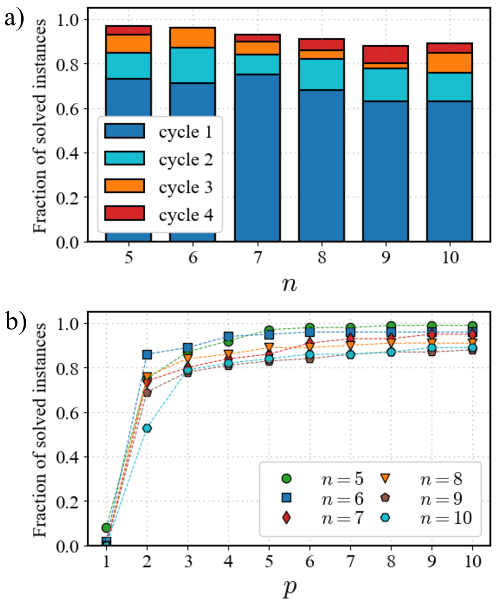
Figure 4: Fraction of SK instances (10) solved with the ion native QAOA for different system sizes $n$ and plotted a) after each cycle of training $p=n$ layered QAOA circuit and b) after the 4-th cycle of training as a function of the QAOA circuit depth $p$.

For each number of qubits, 100 random instances of the SK model are sampled with $K_{ij}\sim\mathcal{N}(0,1)$. Several training cycles are performed for the sampled instances. Each cycle consists of identifying hyperparameters for every specific instance, followed by the Hamiltonian minimization using the obtained ansatzes. After each cycle, we evaluate the fraction of solved instances using a $p=n$ layer circuit. Each subsequent cycle is run only for the remaining unsolved instances.

Fig. 4a demonstrates the fraction of solved SK instances evaluated after each cycle of training for different number of qubits $n$. As one can see, after a single training cycle, 63–75% of sampled instances are solved. This is improved by running additional cycles: after running four of them, the fraction of solved instances increases to 88–97%. Note that reaching the same fraction of solved instances might require a number of training cycles that increases with the system size $n$. This can be explained by the fact that it becomes harder to optimize the energy (7) for larger $n$.

Fig. 4b presents the numerical results for the fraction of solved SK instances calculated as a function of the QAOA circuit depth for $n=5$–10 qubits and $p\leq 10$ layers. These results are obtained for hyperparameters $\bm{A}$ computed in four cycles of training for random instances as described above. For all considered problem sizes $n$, the fraction of solved instances experiences a sharp jump at $p=2$ — in accordance with the results of state preparation — increasing up to 89–99% for circuit depth $p=10$. Interestingly, for every problem size $n$ it can be observed that $p=4$ layers of the ion native ansatz are sufficient to solve most instances (greater than $80\%$). We have also checked the heuristic scalability by running the same set of experiments for $n=15$ qubits, where $50\%$ of the instances have been solved after a single cycle of training, increasing to $76\%$ after four cycles. This, together with the results illustrated in Fig. 4a, demonstrates no significant degradation of the heuristic performance upon the system size increase.

Finally, Fig. 5 compares the performance of the ion native QAOA with the best found hyperparameters and standard QAOA, solving the same pool of sampled SK instances with the same settings of the layerwise optimization procedure (Appendix C). Two key observations can be made. First, for a given problem size, the ion native QAOA strongly outperforms the standard one in terms of the fraction of solved instances. Compared to the ion native implementation, standard QAOA exhibits a much slower performance improvement as depth $p$ increases. Second, the ion native QAOA experiences a lesser performance degradation as the system size increases.

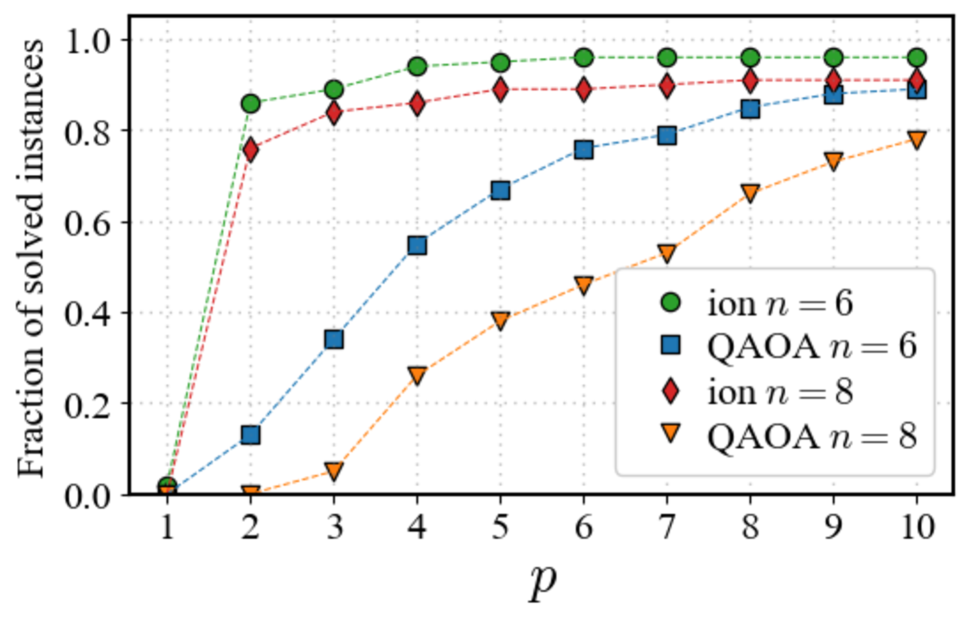
Figure 5: Fraction of SK instances (10) for $n=6$ and 8 qubits solved by the ion native and standard QAOA as a function of circuit depth $p$. The results for the ion-based QAOA are obtained using problem-specific hyperparameters found by the proposed heuristic.

V Conclusions

Digital-analog quantum circuits provide a promising tool for reducing algorithms dependence on limited fidelity entangling gates. A notable example of this approach is the ion based quantum architecture, as it naturally supports the long range all-to-all interaction [58]. The latter can be controlled on a real quantum device by varying intensities of the applied laser fields. As evidenced by a recent proposal of the ion native ansatz for combinatorial optimization [66], the algorithmic performance strongly depends on the choice of interaction parameters (called ansatz hyperparameters $\bm{A}$). Identifying a suitable configuration of these hyperparameters, however, can itself be a challenging problem.

In this work, we addressed the problem of identifying hyperparameters of the ion native ansatz suitable for minimizing specific problem Hamiltonians. We proposed a heuristic for searching a well-trainable ansatz configuration based on a single layer optimization. The heuristic uses the block coordinate descent method for minimizing the energy alternately over variational and hyper- parameters. The obtained hyperparameters are then rescaled by a factor which maximizes the fraction of variational parameters space below a certain energy threshold. This allows to eliminate a potential narrow gorge problem in the optimization landscape [79]. The proposed heuristic has a significant advantage as it requires evaluating the energy only for a single layer, which has a low computational cost and is relativelly easy to access in an experiment.

We benchmarked the proposed heuristic on random instances of the Sherrington-Kirkpatrick (SK) model with interaction couplings sampled from the standard normal distribution. We demonstrated that our heuristic obtains ansatz hyperparameters that provide a favorable single layer cost landscape, where the energy behaves almost like a convex function with a single global minimum located in a pronounced well. These high trainability properties are extended to deeper circuits, ameliorating the optimization. Similar results were observed for MAX-CUT on random and regular graphs. In addition, we observed the interplay between the trainability and expressibility of different ion native ansatz configurations. By choosing a problem-specific configuration of $\bm{A}$, we restrict the ansatz expressibility, tuning it to prepare specific quantum states out of the whole Hilbert space.

We systematically studied the heuristic performance on random SK instances for system sizes $n$ up to 15 qubits. For each $n$, the performance was measured as the fraction of 100 sampled SK instances solved in the ion-based QAOA with problem-specific hyperparameters. We showed that this fraction, evaluated at the circuit depth $p=n$, increases after each training cycle. After four of these cycles, 88–97% of problem instances were solved at $p=n$ layers for $n$ from 5 to 10. Moreover, we calculated the fraction of solved SK instances as a function of $p$ and found that more than 80% of all instances can be solved using no more than $p=4$ layers for the considered system sizes. Identical experiments for $n=15$ qubits demonstrated no significant performance degradation.

Finally, the obtained numerical results were compared to the performance of standard QAOA. For a given problem size, we found that the ion native QAOA strongly outperforms the standard one in terms of the fraction of solved instances. Compared to the standard implementation, ion native QAOA, enhanced with the proposed heuristic, exhibits a much faster performance improvement with circuit depth. Moreover, the ion native QAOA experiences a lesser performance degradation as the system size increases.

The intuition behind the proposed heuristic can be understood as follows. By minimizing the expectation value at depth one, it identifies an ansatz capable of boosting the amplitudes of certain low energy states. Consequently, at larger depths the ansatz can approximate one of those low energy states. As a result, the prepared state can be close to the ground state — allowing us to classify an instance as solved — or close to one of the low energy excited states, which would be considered a suboptimal solution. Indeed, we observed that training cycles which did not succeed in preparing the true solution were approximating one of the low energy excited states. In this work, we focused on the preparation of the ground state, yet in the regime of a large scale combinatorial optimization these suboptimal solutions can equally be considered acceptable. Thus, the heuristic can be expected to be useful for large scale problem instances as well. This also allows us to conjecture that a similar approach can also be implemented for other problems, not limited to combinatorial optimization.

We believe these results demonstrate the advantages of the ion native ansatz which, in addition to being naturally implementable on a trapped ions quantum computer, can be tuned to drastically improve the algorithmic performance as well as to reduce the circuit depth required to solve a problem. This is crucial for implementing variational quantum algorithms on near-term quantum computers.

Data Availability Statement

The data that support the findings of this study are available from the corresponding author upon a reasonable request.

Appendix A Effective Ising Hamiltonian for laser-ions interaction

A chain of $n$ ions in a linear trap interacting with a laser field of frequency $\omega$ is described by the Hamiltonian $H=H_{0}+H_{\rm I}$ [85], where (here and hereafter, we set $\hbar\equiv~1$)

$$H_{0} = \sum_{m=1}^{n}\omega_{m}\left(a_{m}^{\dagger}a_{m}+1/2\right)+\frac{\omega_{0}}{2}\sum_{i=1}^{n}Z_{i},$$ (15)

$$H_{\rm I} = \sum_{i=1}^{n}\Omega_{i}X_{i}\cos(kx_{i}-\omega t+\varphi).$$ (16)

The first term in $H_{0}$ in Eq. (15) describes the ions motion in terms of the normal mode phonon creation and annihilation operators $a_{m}^{\dagger}$ and $a_{m}$, respectivelly, at frequency $\omega_{m}$. The second term in Eq. (15) describes the electronic state of isolated individual ions, where $\omega_{0}=E_{1}-E_{0}$ is the energy difference between the excited and ground states. The Hamiltonian $H_{\rm I}$ in Eq. (16) corresponds to the laser-ion interaction, where $k$ and $\varphi$ are the wave number and phase of a laser beam, while $\Omega_{i}$ and $x_{i}$ are the Rabi frequency and position of the $i$-th ion. The ions positions are expressed in terms of phonon operators as

$$k\cdot x_{i}=\sum_{m}\eta_{i}^{m}\left(a_{m}e^{-i\omega_{m}t}+a^{\dagger}_{m}e^{i\omega_{m}t}\right),$$ (17)

where $\eta_{i}^{m}$ is the Lamb-Dicke parameter for the coupling between the $i$-th ion and $m$-th normal mode. In Eqs. (15) and (16), $Z_{i}$ and $X_{i}$ denote the Pauli operators acting on the electronic state of the $i$-th ion.

A standard approach for implementing two-qubit operations in this setting consists of using a pair of noncopropagating laser beams with bichromatic beatnotes at frequencies $\omega=\omega_{0}\pm\mu$ symmetrically detuned by $\mu$ [86]. We assume that their wave vectors difference $\bm{\delta k}$ is aligned along the $x$ direction of ions motion. Then, under the rotating wave approximation ($\omega_{0}\gg\mu$) and within the Lamb-Dicke limit ($\delta k\langle x_{i}\rangle\ll 1$), the laser-ion Hamiltonian $H_{\rm I}$ in the interaction picture with respect to $H_{0}$ reduces to [87]

$$H_{\mathrm{I}}(t)=\sum_{i}\Omega_{i}\left(\delta k\cdot x_{i}\right)X_{i}\sin(\mu t).$$ (18)

The evolution operator under the Hamiltonian (18) can be obtained by means of the Magnus expansion terminated after the first two terms [74, 88]:

$$U_{\mathrm{I}}(\tau)=\exp\left[\sum_{i}\phi_{i}(\tau)X_{i}-i\sum_{i<j}\chi_{ij}(\tau)X_{i}X_{j}\right].$$ (19)

The first term in the exponent in Eq. (19),

$$\phi_{i}(\tau)=\sum_{m}\left[\alpha_{i,m}(\tau)a_{m}^{\dagger}-\alpha_{i,m}^{*}(\tau)a_{m}\right],$$ (20)

represents spin-dependent displacements of the $m$-th normal mode through phase space by an amount of $\alpha_{i,m}(\tau)$. The second term in Eq. (19) describes a spin-spin interaction between the $i$-th and $j$-th ions with coupling $\chi_{ij}(\tau)$. The explicit expressions for $\alpha_{i,m}(\tau)$ and $\chi_{ij}(\tau)$ are cumbersome, hence we refer to [74]. In what follows, we focus on the dispersive regime ($|\mu-\nu_{m}|\gg\Omega_{i}\eta_{i}^{m}$), where the phonons are only virtually excited as the displacements become negligible ($\alpha_{i,n}(\tau)\ll 1$) [74]. As the result, the evolution operator (19) takes the form $U_{I}(\tau)=e^{-i\tau H_{\rm I}}$, where $H_{\rm I}$ reduces to the effective fully-connected Ising Hamiltonian (1) [74, 58].

Appendix B Calculation of Ising couplings in the ion Hamiltonian

In order to calculate the matrix $C_{ij}$ of phonon contribution to the Ising couplings (2) in the ion Hamiltonian, we simulated the motion of trapped ions to get the phonon frequencies $\omega_{m}$ and Lamb-Dicke parameters $\eta_{i}^{m}$ [89]. This was done using the standard method [74, 90].

Let us consider a chain of $n$ ions confined in a linear trap. The motion of ions is described by the potential

$$V=\sum_{\xi}\sum_{i}\frac{M\omega_{\xi}\,\xi_{i}^{2}}{2}+\sum_{i\neq j}\frac{e^{2}}{4\pi\epsilon_{0}r_{ij}},$$ (21)

which accounts for the external trapping potential as well as the Coulomb interaction between the ions. In Eq. (21), $M$ is the ion mass, $\omega_{\xi}$ is the center-of-mass trap frequency along the direction $\xi=\{x,y,z\}$, and $r_{ij}$ is the distance between the $i$-th and $j$-th ions. Typically, $\omega_{x}\sim\omega_{y}\gg\omega_{z}$, and one has a linear geometry with the chain of ions stretched along the $z$ axis. The equilibrium positions $z_{i}^{0}$ ($x_{i}^{0}=y_{i}^{0}\equiv 0$) of ions are calculated by minimizing the potential (21) over $z_{i}$:

$$\tilde{V}=\sum_{i}u_{i}^{2}+\sum_{i\neq j}\frac{1}{|u_{i}-u_{j}|}\to\min_{u_{i}},$$ (22)

where $u_{i}\equiv z_{i}^{0}/\ell$ are the dimensionless equilibrium positions, and $\ell=\sqrt[3]{e^{2}/(4\pi\epsilon_{0}M\omega_{z}^{2})}$ sets the scale of ion spacings in the linear chain.

The phonon frequencies are obtained through diagonalization of the potential $V$ in the harmonic approximation. Introducing the ions displacements $q^{\xi}_{i}=\xi_{i}-\xi_{i}^{0}$, one can expand the potential (21) around the equilibrium positions $\xi^{0}_{i}=(x_{i}^{0},y_{i}^{0},z_{i}^{0})$ as

$$V=\frac{M\omega_{z}^{2}}{2}\sum_{\xi}\sum_{ij}A_{ij}^{\xi}q^{\xi}_{i}q^{\xi}_{j}.$$ (23)

The matrix elements $A_{ij}^{\xi}=\left[\partial^{2}V/\partial\xi_{i}\partial\xi_{j}\right]|_{\xi_{i}=\xi_{i}^{0}}$ in the expansion (23) are completely determined by $u_{i}$:

$$A_{ij}^{\xi}=\begin{cases}r_{\xi}^{2}+\sum_{k=1,k\neq j}^{n}a_{\xi}/|u_{j}-u_{k}|^{3},\quad i=j,\\ -a_{\xi}/|u_{i}-u_{j}|^{3},\quad i\neq j,\end{cases}$$ (24)

where $r_{\xi}=\omega_{\xi}/\omega_{z}$, $a_{x}=a_{y}=-1$ and $a_{z}=2$. The eigen frequencies $\omega_{\xi,m}=\sqrt{\lambda_{\xi,m}}\,\omega_{\xi}$ and eigen vectors $\bm{b}^{\xi,m}$ for both the radial ($\xi=x$) and axial ($\xi=z$) normal modes $m$ are obtained from diagonalization of the matrix (24),

$$A^{\xi}\bm{b}^{\xi,m}=\lambda_{\xi,m}\,\bm{b}^{\xi,m},\quad m=1,\ldots,n.$$ (25)

Note that the normal modes along $x$ and $y$ directions are degenerate, so it is enough to consider only the $x$-modes.

We diagonalized the matrix (24) to calculate its phonon eigen frequencies $\omega_{m}\equiv\sqrt{\lambda_{x,m}}\,\omega_{x}$ and eigen vectors $\bm{b}^{m}\equiv\bm{b}^{x,m}$ for the radial normal modes ($\xi=x$). The contribution from the axial normal modes ($\xi=z$) was not taken into account due to the geometry of chosen laser beams. The Lamb-Dicke parameters were calculated then as

$$\eta_{i}^{m}=\delta k\sqrt{\hbar/(2M\omega_{m})}\,b_{i}^{m}.$$ (26)

Here, $\delta k=2\pi/\lambda$, where $\lambda$ is the wavelength of a laser beam. After that, we substituted the frequencies $\omega_{m}$ and Lamb-Dicke parameters $\eta_{i}^{m}$ into Eq. (2) to calculate the matrix $C_{ij}$ for the Ising couplings in the ion Hamiltonian for a given laser detuning $\mu$.

Appendix C Numerical details

For each number of ions (qubits) $n$, we simulated a chain of ⁴⁰Ca⁺ ions of the atomic mass $M=39.96$ a.m.u. The radial and axial frequencies for a linear trap were set to $\omega_{x}/2\pi=1$ MHz and $\omega_{z}/2\pi=0.15$ MHz, respectively. The wavelength of a laser beam was set to $\lambda=729.15$ nm. After calculating the phonon frequencies $\omega_{m}$ and Lamb-Dicke parameters $\eta_{i}^{m}$ as described in Appendix B, we evaluated the matrix $C_{ij}$ using Eq. (2) with the laser detuning fixed at $\mu=\omega_{x}+2\pi\delta\nu$, where $\delta\nu=1$ kHz. The maximal Rabi frequency in Eq. (3) was chosen equal to $\Omega_{\max}/2\pi=30$ kHz for all $n$ (except for 10 and 15 qubits, where we used 50 kHz). This choice of $\Omega_{\max}$ allowed to normalize the matrix (3) of Ising couplings such that its maximal element was about $J_{\max}\sim 1$ kHz. The latter implies propagation times with the ion Hamiltonian $H_{\rm I}$ of the order of several milliseconds [66].

For each sampled instance of the SK model (10), we run the heuristic proposed in Sec. III to obtain a problem-specific configuration $\bm{A}$ of the ion native ansatz by minimizing the energy (7) for a single layer alternately over variational and hyper- parameters. On each BCD iteration $k$, we minimized the energy $F(\bm{\theta})=E(\bm{\theta},\bm{A}_{k})$ over the block of variational parameters $\bm{\theta}=(\beta,\gamma)\in\Theta$ using the approach inspired by [91]. We evaluated the energy $F(\bm{\theta})$ on a $25\times 25$ discretization grid introduced on $\Theta$ and stored these values in the form of a matrix $F_{ij}=F(\beta_{i},\gamma_{j})$. Then, we found the position of its minimal element, $(i_{*},j_{*})=\operatorname*{arg\,min}_{i,j}F_{ij}$, and used $(\beta_{i_{*}},\gamma_{j_{*}})$ as a starting point for the standard gradient-based Broyden-Fletcher-Goldfarb-Shanno (BFGS) [92] optimizer, which locally converged to the optimal solution $\bm{\theta}_{k}$. This technique allows to overcome optimization issues and avoid local minima. For minimizing the energy $E(\bm{\theta}_{k},\bm{A})$ over the block of hyperparameters $\bm{A}\in[-1,1]^{n}$, we used the efficient derivative-free Powell’s conjugate directions method [93]. Both optimizers, L-BFGS-B and Powell’s, were taken as implemented in the SciPy library [94] using default settings.

For each sampled SK instance, we searched the optimal scaling factor $\alpha^{*}$ for obtained hyperparameters $\bm{A}^{*}$ to maximize the fraction of parameters space below some certain value. The latter was estimated by constructing the following cost function $f(\alpha)$. First, we evaluated the energy $E(\bm{\theta},\bm{A}^{*})$ on a $25\times 25$ discretization grid on $\Theta$ and found its global minimum, $E_{*}=\min_{i,j}E_{ij}$. Then, for a given $\alpha$ we similarly evaluated the energy $E(\bm{\theta},\alpha\bm{A}^{*})$ for rescaled hyperparameters and stored it in the form of a matrix $E_{ij}^{\alpha}$. Generally, its minimal element, $E_{*}^{\alpha}=\min_{i,j}E^{\alpha}_{ij}$, should be close to $E_{*}$. However, it is possible to rescale the energy landscape such that the global minimum moves outside of the parameter space $\Theta$. So, if $|E_{*}-E_{*}^{\alpha}|>\epsilon$ or any of new hyperparameters $\alpha\bm{A}^{*}$ became out of range $[-1,1]$, we assumed that $f(\alpha)$ returns $-1$. Otherwise, we counted the number of matrix elements below some energy level, $M=|\{(i,j):|E_{ij}^{\alpha}-E_{*}^{\alpha}|<\lambda|E_{*}^{\alpha}|\}|$, and assumed that $f(\alpha)$ returns the desired fraction of parameter space $\Theta$ estimated as $M/M_{\rm tot}$, where $M_{\rm tot}=25^{2}$ is the total number of matrix elements. The constructed cost function $f(\alpha)$ was maximized by means of the golden-section search method. The parameters $\epsilon$ and $\lambda$ were set both equal to $0.05$.

The optimization of the QAOA energy (6) was performed by means of a layerwise inspired heuristic [51]. This method iterates over the QAOA circuit depth $p$ starting from a single layer ($p=1$) that is optimized with respect to two variational parameters. On each iteration, a new layer is added and optimized separately over its variational parameters, while keeping all other parameters from the previous layers fixed. This step is followed by the simultaneous optimization over all variational parameters for the whole QAOA circuit. For optimization, we once again used the L-BFGS-B optimizer. On each step of this layerwise training heuristic, we started the optimizer from 25 random initial points sampled uniformly in the parameter space and chose the best result. In order to find a global minimum, we performed 10 runs of this layerwise training for each circuit depth $p$ in our QAOA simulations choosing the result with the smallest energy (6).

Appendix D State preparation problem

Minimization of a diagonal problem Hamiltonian requires one to find an approximation to a bit string state $\ket{t}$ of the lowest energy. Thus, to estimate the depth sufficient to solve an arbitrary combinatorial problem, one only needs to find the depth of a circuit that can prepare an arbitrary bit string state. For the case of a $\mathbb{Z}_{2}$-symmetric ansatz and problem Hamiltonian, the latter translates to preparing a GHZ-like states of the form $\dfrac{1}{\sqrt{2}}(\ket{t}+X^{\otimes n}\ket{t})$.

Importantly, the ansatz (4) possesses certain symmetries with respect to hyperparameters. Specifically, given a state $\ket{\psi(\bm{\beta},\bm{\gamma},A_{j})}$, prepared using ansatz (4) with hyperparameters $\{A_{j}\}$, one can note

$$X_{m}\ket{\psi(\bm{\beta},\bm{\gamma},A_{j})}=\ket{\psi(\bm{\beta},\bm{\gamma},(-1)^{\delta_{jm}}A_{j})}.$$ (27)

In other words, flipping the $m$-th bit in the prepared state is equivalent to flipping the sign of $A_{m}$. By extension, flipping several qubits is equivalent to changing the signs of the corresponding hyperparameters. As a consequence, the same circuit depth is required to prepare any bit string $\ket{t}$ — or rather its symmetrized version $\dfrac{1}{\sqrt{2}}\big{(}\ket{t}+X^{\otimes n}\ket{t}\big{)}$, which respects the $\mathbb{Z}_{2}$ symmetry of the ansatz  [66]. Thus, the minimization of all diagonal Hamiltonians of a given size requires the same circuit depth, at least in principle. This argument evidently ignores how easy it is to train such circuits as well as how to properly adjust the ansatz hyperparameters. Nevertheless, this fact can be used to establish a bound on the required depth to solve specific problems.

Due to property (27) of the ion native ansatz, one can restrict the problem to the preparation of any of these states. Therefore, here we maximize the overlap with the GHZ state,

$$|\innerproduct{\psi_{p}(\bm{\beta},\bm{\gamma})}{\rm GHZ}|^{2}\to\max_{\bm{\beta},\bm{\gamma}},$$ (28)

where $\ket{\rm GHZ}=(\ket{0}^{\otimes n}+\ket{1}^{\otimes n})/\sqrt{2}$.

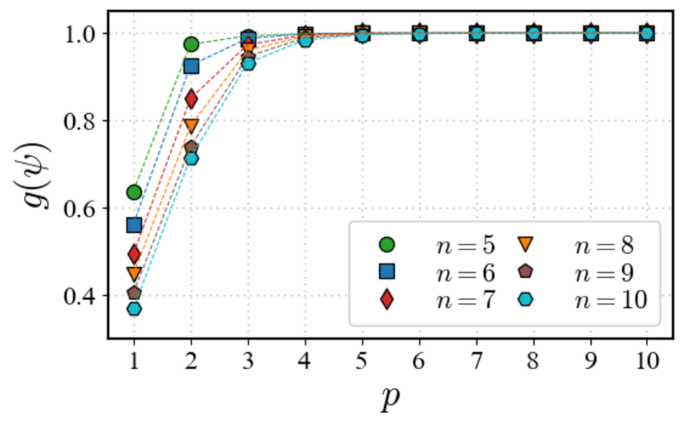
Figure 6: Ground state overlap $g(\psi)$ as a function of circuit depth $p$ calculated by the ion native QAOA when solving the state preparation problem (28) for different system sizes $n$. For each $n$, the results are obtained using problem-specific hyperparameters found by the proposed heuristic.

Following our numerics for the SK Hamiltonian (10) in Sec. IV, we considered system sizes $n$ of $5$–$10$ qubits. We use the proposed heuristic, by minimizing the Hamiltonian $H_{\rm P}=-(\outerproduct{0}{0}^{\otimes n}+\outerproduct{1}{1}^{\otimes n})$ which, due to the $\mathbb{Z}_{2}$ symmetry, is equivalent to the state preparation problem (28). The heuristic was tuned by setting $\varepsilon=0$ in the convergence criteria (8) to identify ansatz hyperparameters providing the smallest energy (7) (largest overlap (28)) over $m_{\max}=10$ runs. In this setting, the heuristic tried to reach a global minimum of the energy for a single layer. Once the ansatz hyperparameters were identified, we performed ion native QAOA simulations for circuit depths $p$ of up to 10 layers. Fig. 6 shows the ground state overlap $g(\psi)$ calculated as a function of the QAOA circuit depth $p$. As one can see, the QAOA performance slightly decreases with the system size $n$. Nevertheless, $p=2$ layers are already sufficient to reach the ground state overlap of $50\%$ for all considered $n$, while $p=7$ layers guarantee the overlap of $99.9\%$.

References

- Weidenfeller et al. [2022] J. Weidenfeller, L. C. Valor, J. Gacon, C. Tornow, L. Bello, S. Woerner, and D. J. Egger, Scaling of the quantum approximate optimization algorithm on superconducting qubit based hardware, Quantum 6, 870 (2022).
- Ratcliffe et al. [2018] A. K. Ratcliffe, R. L. Taylor, J. J. Hope, and A. R. Carvalho, Scaling trapped ion quantum computers using fast gates and microtraps, Phys. Rev. Lett. 120, 220501 (2018).
- Hegde et al. [2022] S. S. Hegde, J. Zhang, and D. Suter, Toward the speed limit of high-fidelity two-qubit gates, Phys. Rev. Lett. 128, 230502 (2022).
- Mills et al. [2022] A. R. Mills, C. R. Guinn, M. J. Gullans, A. J. Sigillito, M. M. Feldman, E. Nielsen, and J. R. Petta, Two-qubit silicon quantum processor with operation fidelity exceeding 99%, Sci. Adv. 8, eabn5130 (2022).
- Cerezo et al. [2021a] M. Cerezo, A. Arrasmith, R. Babbush, S. C. Benjamin, S. Endo, K. Fujii, J. R. McClean, K. Mitarai, X. Yuan, L. Cincio, et al., Variational quantum algorithms, Nat. Rev. Phys. 3, 625 (2021a).
- Biamonte [2021] J. Biamonte, Universal variational quantum computation, Phys. Rev. A 103, L030401 (2021).
- Parrish et al. [2019] R. M. Parrish, E. G. Hohenstein, P. L. McMahon, and T. J. Martínez, Quantum computation of electronic transitions using a variational quantum eigensolver, Phys. Rev. Lett. 122, 230401 (2019).
- Hempel et al. [2018] C. Hempel, C. Maier, J. Romero, J. McClean, T. Monz, H. Shen, P. Jurcevic, B. P. Lanyon, P. Love, R. Babbush, A. Aspuru-Guzik, R. Blatt, and C. F. Roos, Quantum chemistry calculations on a trapped-ion quantum simulator, Phys. Rev. X 8, 031022 (2018).
- Kandala et al. [2017] A. Kandala, A. Mezzacapo, K. Temme, M. Takita, M. Brink, J. M. Chow, and J. M. Gambetta, Hardware-efficient variational quantum eigensolver for small molecules and quantum magnets, Nature 549, 242 (2017).
- Peruzzo et al. [2014] A. Peruzzo, J. McClean, P. Shadbolt, M.-H. Yung, X.-Q. Zhou, P. J. Love, A. Aspuru-Guzik, and J. L. O’Brien, A variational eigenvalue solver on a photonic quantum processor, Nat. Commun. 5, 4213 (2014).
- Cade et al. [2020] C. Cade, L. Mineh, A. Montanaro, and S. Stanisic, Strategies for solving the Fermi-Hubbard model on near-term quantum computers, Phys. Rev. B 102, 235122 (2020).
- Zeng et al. [2021] J. Zeng, Z. Wu, C. Cao, C. Zhang, S.-Y. Hou, P. Xu, and B. Zeng, Simulating noisy variational quantum eigensolver with local noise models, Quantum Engineering 3, e77 (2021).
- Kardashin et al. [2021] A. Kardashin, A. Pervishko, J. Biamonte, and D. Yudin, Numerical hardware-efficient variational quantum simulation of a soliton solution, Phys. Rev. A 104, L020402 (2021).
- Uvarov et al. [2020] A. Uvarov, J. D. Biamonte, and D. Yudin, Variational quantum eigensolver for frustrated quantum systems, Phys. Rev. B 102, 075104 (2020).
- Uvarov et al. [2024] A. Uvarov, D. Rabinovich, O. Lakhmanskaya, K. Lakhmanskiy, J. Biamonte, and S. Adhikary, Mitigating quantum gate errors for variational eigensolvers using hardware-inspired zero-noise extrapolation, Phys. Rev. A 110, 012404 (2024).
- Yuan et al. [2019] X. Yuan, S. Endo, Q. Zhao, Y. Li, and S. C. Benjamin, Theory of variational quantum simulation, Quantum 3, 191 (2019).
- Cirstoiu et al. [2020] C. Cirstoiu, Z. Holmes, J. Iosue, L. Cincio, P. J. Coles, and A. Sornborger, Variational fast forwarding for quantum simulation beyond the coherence time, npj Quantum Inf 6, 82 (2020).
- Gibbs et al. [2022] J. Gibbs, K. Gili, Z. Holmes, B. Commeau, A. Arrasmith, L. Cincio, P. J. Coles, and A. Sornborger, Long-time simulations for fixed input states on quantum hardware, npj Quant Inf 8, 135 (2022).
- Endo et al. [2020] S. Endo, J. Sun, Y. Li, S. C. Benjamin, and X. Yuan, Variational quantum simulation of general processes, Phys. Rev. Lett. 125, 010501 (2020).
- Farhi et al. [2014a] E. Farhi, J. Goldstone, and S. Gutmann, A Quantum Approximate Optimization Algorithm (2014a), arXiv:1411.4028 [quant-ph] .
- Morales et al. [2020] M. E. S. Morales, J. D. Biamonte, and Z. Zimborás, On the universality of the quantum approximate optimization algorithm, Quantum Information Processing 19, 291 (2020).
- Farhi et al. [2014b] E. Farhi, J. Goldstone, and S. Gutmann, A Quantum Approximate Optimization Algorithm Applied to a Bounded Occurrence Constraint Problem (2014b), arXiv:1412.6062 [quant-ph] .
- Wang et al. [2018] Z. Wang, S. Hadfield, Z. Jiang, and E. G. Rieffel, Quantum approximate optimization algorithm for maxcut: A fermionic view, Phys. Rev. A 97, 022304 (2018).
- Lloyd [2018] S. Lloyd, Quantum approximate optimization is computationally universal (2018), arXiv:1812.11075 [quant-ph] .
- Zhou et al. [2020] L. Zhou, S.-T. Wang, S. Choi, H. Pichler, and M. D. Lukin, Quantum Approximate Optimization Algorithm: Performance, Mechanism, and Implementation on Near-Term Devices, Phys. Rev. X 10, 021067 (2020).
- Claes and van Dam [2021] J. Claes and W. van Dam, Instance Independence of Single Layer Quantum Approximate Optimization Algorithm on Mixed-Spin Models at Infinite Size, Quantum 5, 542 (2021).
- Wauters et al. [2020] M. M. Wauters, G. B. Mbeng, and G. E. Santoro, Polynomial scaling of the quantum approximate optimization algorithm for ground-state preparation of the fully connected -spin ferromagnet in a transverse field, Phys. Rev. A 102, 062404 (2020).
- Rabinovich et al. [2022a] D. Rabinovich, R. Sengupta, E. Campos, V. Akshay, and J. Biamonte, Progress towards analytically optimal angles in quantum approximate optimisation, Mathematics 10, 2601 (2022a).
- Akshay et al. [2021] V. Akshay, D. Rabinovich, E. Campos, and J. Biamonte, Parameter concentrations in quantum approximate optimization, Phys. Rev. A 104, L010401 (2021).
- Akshay et al. [2020] V. Akshay, H. Philathong, M. E. Morales, and J. D. Biamonte, Reachability deficits in quantum approximate optimization, Phys. Rev. lett. 124, 090504 (2020).
- Campos et al. [2024] E. Campos, D. Rabinovich, and A. Uvarov, Depth scaling of unstructured search via quantum approximate optimization, Phys. Rev. A 110, 012428 (2024).
- Campos et al. [2021] E. Campos, D. Rabinovich, V. Akshay, and J. Biamonte, Training saturation in layerwise quantum approximate optimization, Phys. Rev. A 104, L030401 (2021).
- Khatri et al. [2019] S. Khatri, R. LaRose, A. Poremba, L. Cincio, A. T. Sornborger, and P. J. Coles, Quantum-assisted quantum compiling, Quantum 3, 140 (2019).
- Jones and Benjamin [2022] T. Jones and S. C. Benjamin, Robust quantum compilation and circuit optimisation via energy minimisation, Quantum 6, 628 (2022).
- He et al. [2021] Z. He, L. Li, S. Zheng, Y. Li, and H. Situ, Variational quantum compiling with double Q-learning, New J. Phys. 23, 033002 (2021).
- Liang et al. [2020] J.-M. Liang, S.-Q. Shen, M. Li, and L. Li, Variational quantum algorithms for dimensionality reduction and classification, Phys. Rev. A 101, 032323 (2020).
- McClean et al. [2016] J. R. McClean, J. Romero, R. Babbush, and A. Aspuru-Guzik, The theory of variational hybrid quantum-classical algorithms, New J. Phys. 18, 023023 (2016).
- Benedetti et al. [2019] M. Benedetti, E. Lloyd, S. Sack, and M. Fiorentini, Parameterized quantum circuits as machine learning models, Quantum Sci. Technol. 4, 043001 (2019).
- Verdon et al. [2017] G. Verdon, M. Broughton, and J. Biamonte, A quantum algorithm to train neural networks using low-depth circuits (2017), arXiv:1712.05304 [quant-ph] .
- Mitarai et al. [2018] K. Mitarai, M. Negoro, M. Kitagawa, and K. Fujii, Quantum circuit learning, Phys. Rev. A 98, 032309 (2018).
- Schuld et al. [2019] M. Schuld, V. Bergholm, C. Gogolin, J. Izaac, and N. Killoran, Evaluating analytic gradients on quantum hardware, Phys. Rev. A 99, 032331 (2019).
- Xu et al. [2021] X. Xu, S. C. Benjamin, and X. Yuan, Variational Circuit Compiler for Quantum Error Correction, Phys. Rev. Appl. 15, 034068 (2021).
- Cerezo et al. [2021b] M. Cerezo, A. Sone, T. Volkoff, L. Cincio, and P. J. Coles, Cost function dependent barren plateaus in shallow parametrized quantum circuits, Nat. Commun. 12, 1791 (2021b).
- Gentini et al. [2020] L. Gentini, A. Cuccoli, S. Pirandola, P. Verrucchi, and L. Banchi, Noise-resilient variational hybrid quantum-classical optimization, Phys. Rev. A 102, 052414 (2020).
- Sharma et al. [2020] K. Sharma, S. Khatri, M. Cerezo, and P. J. Coles, Noise resilience of variational quantum compiling, New Journal of Physics 22, 043006 (2020).
- Cincio et al. [2021] L. Cincio, K. Rudinger, M. Sarovar, and P. J. Coles, Machine Learning of Noise-Resilient Quantum Circuits, PRX Quantum 2, 010324 (2021).
- Harrigan et al. [2021] M. P. Harrigan, K. J. Sung, M. Neeley, K. J. Satzinger, F. Arute, K. Arya, J. Atalaya, J. C. Bardin, R. Barends, S. Boixo, et al., Quantum approximate optimization of non-planar graph problems on a planar superconducting processor, Nat. Phys. 17, 332 (2021).
- Guerreschi and Matsuura [2019] G. G. Guerreschi and A. Y. Matsuura, QAOA for Max-Cut requires hundreds of qubits for quantum speed-up, Sci Rep 9, 1 (2019).
- Pagano et al. [2020] G. Pagano, A. Bapat, P. Becker, K. S. Collins, A. De, P. W. Hess, H. B. Kaplan, A. Kyprianidis, W. L. Tan, C. Baldwin, et al., Quantum approximate optimization of the long-range Ising model with a trapped-ion quantum simulator, Proc. Natl. Acad. Sci. 117, 25396 (2020).
- Rabinovich et al. [2024] D. Rabinovich, E. Campos, S. Adhikary, E. Pankovets, D. Vinichenko, and J. Biamonte, Robustness of variational quantum algorithms against stochastic parameter perturbation, Phys. Rev. A 109, 042426 (2024).
- Akshay et al. [2022] V. Akshay, H. Philathong, E. Campos, D. Rabinovich, I. Zacharov, X.-M. Zhang, and J. D. Biamonte, Circuit depth scaling for quantum approximate optimization, Phys. Rev. A 106, 042438 (2022).
- Yu et al. [2022] J. Yu, J. C. Retamal, M. Sanz, E. Solano, and F. Albarrán-Arriagada, Superconducting circuit architecture for digital-analog quantum computing, EPJ Quantum Technology 9, 1 (2022).
- Garcia-de Andoin et al. [2024] M. Garcia-de Andoin, Á. Saiz, P. Pérez-Fernández, L. Lamata, I. Oregi, and M. Sanz, Digital-analog quantum computation with arbitrary two-body hamiltonians, Physical Review Research 6, 013280 (2024).
- Martin et al. [2020] A. Martin, L. Lamata, E. Solano, and M. Sanz, Digital-analog quantum algorithm for the quantum fourier transform, Physical Review Research 2, 013012 (2020).
- Gonzalez-Raya et al. [2021] T. Gonzalez-Raya, R. Asensio-Perea, A. Martin, L. C. Céleri, M. Sanz, P. Lougovski, and E. F. Dumitrescu, Digital-analog quantum simulations using the cross-resonance effect, PRX Quantum 2, 020328 (2021).
- Zhang et al. [2017] J. Zhang, G. Pagano, P. W. Hess, A. Kyprianidis, P. Becker, H. Kaplan, A. V. Gorshkov, Z.-X. Gong, and C. Monroe, Observation of a many-body dynamical phase transition with a 53-qubit quantum simulator, Nature 551, 601 (2017).
- Maier et al. [2019] C. Maier, T. Brydges, P. Jurcevic, N. Trautmann, C. Hempel, B. P. Lanyon, P. Hauke, R. Blatt, and C. F. Roos, Environment-assisted quantum transport in a 10-qubit network, Phys. Rev. Lett. 122, 050501 (2019).
- Monroe et al. [2021] C. Monroe, W. C. Campbell, L.-M. Duan, Z.-X. Gong, A. V. Gorshkov, P. W. Hess, R. Islam, K. Kim, N. M. Linke, G. Pagano, P. Richerme, C. Senko, and N. Y. Yao, Programmable quantum simulations of spin systems with trapped ions, Rev. Mod. Phys. 93, 025001 (2021).
- Richerme et al. [2014] P. Richerme, Z.-X. Gong, A. Lee, C. Senko, J. Smith, M. Foss-Feig, S. Michalakis, A. V. Gorshkov, and C. Monroe, Non-local propagation of correlations in quantum systems with long-range interactions, Nature 511, 198 (2014).
- Smith et al. [2016] J. Smith, A. Lee, P. Richerme, B. Neyenhuis, P. W. Hess, P. Hauke, M. Heyl, D. A. Huse, and C. Monroe, Many-body localization in a quantum simulator with programmable random disorder, Nat. Phys. 12, 907 (2016).
- Senko et al. [2014] C. Senko, J. Smith, P. Richerme, A. Lee, W. C. Campbell, and C. Monroe, Coherent imaging spectroscopy of a quantum many-body spin system, Science 345, 430 (2014).
- Parra-Rodriguez et al. [2020] A. Parra-Rodriguez, P. Lougovski, L. Lamata, E. Solano, and M. Sanz, Digital-analog quantum computation, Physical Review A 101, 022305 (2020).
- Headley et al. [2022] D. Headley, T. Müller, A. Martin, E. Solano, M. Sanz, and F. K. Wilhelm, Approximating the quantum approximate optimization algorithm with digital-analog interactions, Physical Review A 106, 042446 (2022).
- Zhuang et al. [2024] J.-Z. Zhuang, Y.-K. Wu, and L.-M. Duan, Hardware-efficient variational quantum algorithm in a trapped-ion quantum computer, Phys. Rev. A 110, 062414 (2024).
- Kokail et al. [2019] C. Kokail, C. Maier, R. van Bijnen, T. Brydges, M. K. Joshi, P. Jurcevic, C. A. Muschik, P. Silvi, R. Blatt, C. F. Roos, et al., Self-verifying variational quantum simulation of lattice models, Nature 569, 355 (2019).
- Rabinovich et al. [2022b] D. Rabinovich, S. Adhikary, E. Campos, V. Akshay, E. Anikin, R. Sengupta, O. Lakhmanskaya, K. Lakhmanskiy, and J. Biamonte, Ion-native variational ansatz for quantum approximate optimization, Phys. Rev. A 106, 032418 (2022b).
- Holmes et al. [2022] Z. Holmes, K. Sharma, M. Cerezo, and P. J. Coles, Connecting Ansatz Expressibility to Gradient Magnitudes and Barren Plateaus, PRX Quantum 3, 010313 (2022).
- Anschuetz and Kiani [2022] E. R. Anschuetz and B. T. Kiani, Quantum variational algorithms are swamped with traps, Nat. Commun. 13, 7760 (2022).
- Tseng [2001] P. Tseng, Convergence of a Block Coordinate Descent Method for Nondifferentiable Minimization, J. Optim. Theory Appl. 109, 475 (2001).
- Panchenko [2012] D. Panchenko, The Sherrington-Kirkpatrick model: an overview, J. Stat. Phys. 149, 362 (2012).
- Sherrington and Kirkpatrick [1975] D. Sherrington and S. Kirkpatrick, Solvable model of a spin-glass, Phys. Rev. Lett. 35, 1792 (1975).
- Pogorelov et al. [2021] I. Pogorelov, T. Feldker, C. D. Marciniak, L. Postler, G. Jacob, O. Krieglsteiner, V. Podlesnic, M. Meth, V. Negnevitsky, M. Stadler, B. Höfer, C. Wächter, K. Lakhmanskiy, R. Blatt, P. Schindler, and T. Monz, Compact ion-trap quantum computing demonstrator, PRX Quantum 2, 020343 (2021).
- Wright et al. [2019] K. Wright, K. M. Beck, S. Debnath, J. M. Amini, Y. Nam, N. Grzesiak, J.-S. Chen, N. C. Pisenti, M. Chmielewski, C. Collins, K. M. Hudek, J. Mizrahi, J. D. Wong-Campos, S. Allen, J. Apisdorf, P. Solomon, M. Williams, A. M. Ducore, A. Blinov, S. M. Kreikemeier, V. Chaplin, M. Keesan, C. Monroe, and J. Kim, Benchmarking an 11-qubit quantum computer, Nature Communications 10, 5464 (2019).
- Zhu et al. [2006a] S.-L. Zhu, C. Monroe, and L.-M. Duan, Trapped Ion Quantum Computation with Transverse Phonon Modes, Phys. Rev. Lett. 97, 050505 (2006a).
- Wecker et al. [2015] D. Wecker, M. B. Hastings, and M. Troyer, Progress towards practical quantum variational algorithms, Physical Review A 92, 042303 (2015).
- Wiersema et al. [2020] R. Wiersema, C. Zhou, Y. de Sereville, J. F. Carrasquilla, Y. B. Kim, and H. Yuen, Exploring entanglement and optimization within the hamiltonian variational ansatz, PRX quantum 1, 020319 (2020).
- Rajakumar et al. [2024] J. Rajakumar, J. Golden, A. Bärtschi, and S. Eidenbenz, Trainability Barriers in Low-Depth QAOA Landscapes, in Proceedings of the 21st ACM International Conference on Computing Frontiers, CF ’24 (Association for Computing Machinery, New York, 2024) p. 199–206.
- Cerezo et al. [2021c] M. Cerezo, A. Sone, T. Volkoff, L. Cincio, and P. J. Coles, Cost function dependent barren plateaus in shallow parametrized quantum circuits, Nat. Commun. 12, 1791 (2021c).
- Arrasmith et al. [2022] A. Arrasmith, Z. Holmes, M. Cerezo, and P. J. Coles, Equivalence of quantum barren plateaus to cost concentration and narrow gorges, Quantum Sci. Technol. 7, 045015 (2022).
- Farhi et al. [2022] E. Farhi, J. Goldstone, S. Gutmann, and L. Zhou, The Quantum Approximate Optimization Algorithm and the Sherrington-Kirkpatrick Model at Infinite Size, Quantum 6, 759 (2022).
- Sim et al. [2019] S. Sim, P. D. Johnson, and A. Aspuru-Guzik, Expressibility and Entangling Capability of Parameterized Quantum Circuits for Hybrid Quantum-Classical Algorithms, Adv. Quantum Technol. 2, 1900070 (2019).
- Nakaji and Yamamoto [2021] K. Nakaji and N. Yamamoto, Expressibility of the alternating layered ansatz for quantum computation, Quantum 5, 434 (2021).
- [83] E. Anikin, Fast Mølmer-Sørensen gates in trapped-ion quantum processors with compensated carrier transition, https://github.com/EvgAnikin/fast_molmer_sorensen_w_carrier/tree/main.
- Zacharov et al. [2019] I. Zacharov, R. Arslanov, M. Gunin, D. Stefonishin, A. Bykov, S. Pavlov, O. Panarin, A. Maliutin, S. Rykovanov, and M. Fedorov, “Zhores” – Petaflops supercomputer for data-driven modeling, machine learning and artificial intelligence installed in Skolkovo Institute of Science and Technology, Open Eng. 9, 512 (2019).
- Sørensen and Mølmer [2000] A. Sørensen and K. Mølmer, Entanglement and quantum computation with ions in thermal motion, Phys. Rev. A 62, 022311 (2000).
- Lee et al. [2005] P. J. Lee, K.-A. Brickman, L. Deslauriers, P. C. Haljan, L.-M. Duan, and C. Monroe, Phase control of trapped ion quantum gates, J. Opt. B Quantum Semiclassical Opt. 7, S371 (2005).
- Kim et al. [2009] K. Kim, M.-S. Chang, R. Islam, S. Korenblit, L.-M. Duan, and C. Monroe, Entanglement and Tunable Spin-Spin Couplings between Trapped Ions Using Multiple Transverse Modes, Phys. Rev. Lett. 103, 120502 (2009).
- Zhu et al. [2006b] S.-L. Zhu, C. Monroe, and L.-M. Duan, Arbitrary-speed quantum gates within large ion crystals through minimum control of laser beams, Europhys. Lett. 73, 485 (2006b).
- Anikin et al. [2025] E. Anikin, A. Chuchalin, N. Morozov, O. Lakhmanskaya, and K. Lakhmanskiy, Fast molmer-sorensen gates in trapped-ion quantum processors with compensated carrier transition, arXiv preprint arXiv:2501.02387 (2025).
- James [1998] D. F. V. James, Quantum dynamics of cold trapped ions with application to quantum computation, Appl. Phys. B 66, 181 (1998).
- Paradezhenko et al. [2024] G. V. Paradezhenko, A. A. Pervishko, and D. Yudin, Probabilistic tensor optimization of quantum circuits for the problem, Phys. Rev. A 109, 012436 (2024).
- Dennis and Schnabel [1996] J. E. Dennis and R. B. Schnabel, Numerical Methods for Unconstrained Optimization and Nonlinear Equations (SIAM, Philadelphia, 1996).
- Powell [1964] M. J. D. Powell, An efficient method for finding the minimum of a function of several variables without calculating derivatives, Comput. J. 7, 155 (1964).
- Virtanen and et al. [2020] P. Virtanen and et al., SciPy 1.0: Fundamental Algorithms for Scientific Computing in Python, Nature Methods 17, 261 (2020).