Observers seeing gravitational Hilbert spaces: abstract sources for an abstract path integral

Abstract

The gravitational path integral suggests a striking result: the Hilbert space of closed universes in each superselection sector, a so-called $\alpha$-sector, is one-dimensional. We develop an abstract formalism encapsulating recent proposals that modify the gravitational path integral in the presence of observers and allow larger Hilbert spaces to be associated with closed universes. Our formalism regards the gravitational path integral as a map from abstract objects called sources to complex numbers, and introduces additional objects called partial sources, which form sources when glued together. We apply this formalism to treat, on equal footing, universes with spatial boundaries, closed universes with prescribed observer worldlines, and closed universes containing observers entangled with external systems. In these contexts, the relevant gravitational Hilbert spaces contain states prepared by partial sources and can consequently have nontrivial $\alpha$-sectors supporting noncommuting operators. Within our general framework, the positivity of the gravitational inner product implies a bound on the Hilbert space trace of certain positive operators over each $\alpha$-sector. The trace of such operators, in turn, quantifies the effective size of this Hilbert space.

1 Introduction

Recent years have seen significant advancements that clarified some aspects of the black hole information problem. A central development was the discovery of quantum extremal surfaces Penington:2019npb ; Almheiri:2019psf associated with replica wormholes Penington:2019kki ; Almheiri:2019qdq . In particular, a sum over topologies in entropy calculations using the gravitational path integral was found to be crucial for seeing the expected decrease in the number of states of an evaporating black hole, evoking Marolf:2020xie ; Marolf:2020rpm old discussions Coleman:1988cy ; Giddings:1988cx ; Giddings:1988wv of so-called baby universes and $\alpha$-states.

The same rules for the gravitational path integral, however, lead to the striking conclusion that the Hilbert space of closed universes is one-dimensional Marolf:2020xie ; Usatyuk:2024mzs ; Usatyuk:2024isz . This puzzling result is not unrelated to the successes in the black hole context described above Marolf:2020rpm . Indeed, the interior of an evaporated black hole is similar to a closed universe. While the semiclassical descriptions of quantum fields in the interiors of old black holes or in closed universes admit many states, the gravitational path integral suggests that many or all of these states in each case are in fact linearly dependent in quantum gravity Marolf:2020xie ; Marolf:2020rpm ; Akers:2022qdl ; Harlow:2025pvj ; Akers:2025ahe .

In an effort to describe the rich experiences of observers in closed universes, refs. Harlow:2025pvj ; Abdalla:2025gzn have suggested special rules for the inclusion of observers in the gravitational path integral. While these rules recover nontrivial Hilbert spaces for closed universes with observers, they are somewhat ad hoc and are not derived from first principles. Indeed, the rules proposed by refs. Harlow:2025pvj ; Abdalla:2025gzn are distinct and it is unclear whether one proposed set of rules is better than the other, or if either really describe the experiences of an observer. We will instead take an agnostic approach, aiming to identify the general structures shared by the proposals of refs. Harlow:2025pvj ; Abdalla:2025gzn which lead to nontrivial Hilbert spaces in the presence of observers.

In this paper, we develop a general framework in which the gravitational path integral $\zeta:\mathcal{J}\to\mathbb{C}$ is a function from abstract objects $J\in\mathcal{J}$, called sources, to complex numbers. Examples of sources $J$ include boundary manifolds specifying boundary conditions for bulk fields. Other examples, relevant to the prescription of ref. Abdalla:2025gzn , might be boundary manifolds connected by prescribed bulk geodesics. However, to isolate essential features, we will remain as abstract as possible while developing our general framework. We will therefore be interested in identifying general structures and properties which define an abstract set $\mathcal{J}$ of sources and a function $\zeta$ that we refer to as the gravitational path integral.

In particular, we will argue that $\mathcal{J}$ should have the structure of a $*$-algebra, equipped with a commutative multiplication $\sqcup$ which one can view as taking the disjoint union of sources. The gravitational path integral $\zeta:\mathcal{J}\to\mathbb{C}$ is therefore implicitly invariant under permutations of constituent sources in disjoint unions $\sqcup$. This property of the path integral is the underlying structure responsible for the fact that the Hilbert space of closed universes is one-dimensional.

More precisely, by inserting sources $J\in\mathcal{J}$, say in the Euclidean past, we can prepare a Hilbert space $\mathcal{H}_{\emptyset}$ of states associated with bulk slices that do not intersect sources $J$. The slices have no spatial boundary and their topology and local fields vary freely across different configurations in the path integral. We will refer to such freely fluctuating closed universes as baby universes. As we will later review, the commutativity of the $*$-algebra $\mathcal{J}$ implies that the baby universe Hilbert space $\mathcal{H}_{\emptyset}$ decomposes into one-dimensional superselection sectors $\mathcal{H}_{\emptyset}^{\alpha}$ — so-called $\alpha$-sectors. Because they are superselection sectors, each $\mathcal{H}_{\emptyset}^{\alpha}$ can be viewed as the baby universe Hilbert space in a self-contained theory of quantum gravity. Meanwhile, the path integral $\zeta$ and the Hilbert space $\mathcal{H}_{\emptyset}$ describe an ensemble average over these theories labelled by $\alpha$.

As we know concretely from AdS/CFT, if one considers not closed universes but instead universes with spatial boundaries, the gravitational Hilbert space need not be one-dimensional and can support noncommuting operators. In this paper, we will demonstrate that there is a close analogy between universes with spatial boundaries and the prescriptions of refs. Harlow:2025pvj ; Abdalla:2025gzn for including observers in closed universes. The common theme is that Hilbert spaces with nontrivial $\alpha$-sectors supporting noncommuting operators arise from cutting sources for the gravitational path integral.

To formalize this notion, we introduce abstract objects called cuts and partial sources. For each cut $C$, there is a set $\mathcal{J}_{C}$ of partial sources. A defining property of partial sources $J_{C},J_{C}^{\prime}\in\mathcal{J}_{C}$ is that they can be used to construct a complete source $(J_{C}^{\prime}|J_{C})\in\mathcal{J}$ when appropriately glued together across the cut $C$. An example of a partial source is part $J_{C}=\mathscr{N}_{\Sigma}$ of a boundary manifold, itself with boundary $C=\Sigma$. To capture the prescriptions of refs. Abdalla:2025gzn ; Harlow:2015lma for including observers in closed universes, one must consider other examples, obtained from cutting bulk geodesics representing observer worldlines and cutting inner products of external non-gravitational systems.

Before restricting to specific examples, we will see even from our abstract construction that the set $\mathcal{J}_{C}$ of partial sources can be used to prepare a Hilbert space $\mathcal{H}_{C}$ of states which decomposes into $\alpha$-sectors $\mathcal{H}_{C}^{\alpha}$ that are generically not one-dimensional. Conceptually, cuts are crucial for the existence of nontrivial operators in quantum gravity because they are objects to which one can dress such operators. Concretely, we will see that generically noncommuting operators on $\mathcal{H}_{C}^{\alpha}$ can be constructed by gluing certain two-sided partial sources $J_{C\otimes{}C^{*}}\in\mathcal{J}_{C\otimes{}C^{*}}$ to states.

Even though the $\alpha$-sectors $\mathcal{H}_{C}^{\alpha}$ need not be one-dimensional, there are nonetheless useful bounds that one can place on the size of $\mathcal{H}_{C}^{\alpha}$. More precisely, we will show that the positive definiteness of the gravitational inner product implies an upper bound on the Hilbert space trace of certain positive operators over $\mathcal{H}_{C}^{\alpha}$. Together with an estimate of the size of eigenvalues, these traces can then be used to roughly bound the number of states in appropriate windows of eigenvalues. In the case of universes with spatial boundaries, considering the Euclidean boundary time evolution operator $e^{-\beta\,H}$ for example, one recovers the expected bound on the canonical partition function in terms of a path integral with a boundary manifold containing a Euclidean time circle Marolf:2020xie .

Slightly pushing the envelope on ref. Abdalla:2025gzn ’s prescription, the closest analogue of this example would be a bound, on the dimension of the closed universe Hilbert space with one observer, given by a gravitational path integral involving a circular observer worldline. Indeed, this is reminiscent of the path integral studied by ref. Maldacena:2024spf , which emphasized the importance of observers for extracting a state-counting interpretation in de Sitter spacetime. In AdS Jackiw-Teitelboim (JT) gravity minimally coupled to matter and the observer, we will remark that our bound actually seems to fail if the path integral is naively defined in Euclidean signature: the fact that there are no hyperbolic manifolds without boundary at genus zero seems to cause the path integral to undercount the number of states of closed universes with one observer. This leads us to ask whether the AdS JT path integral with a circular observer worldline should have a more sophisticated definition. Alternatively, it may be the case that the partial sources needed to construct circular observer worldlines simply cannot be incorporated into the theory without spoiling the positive definiteness of the gravitational inner product.

Indeed, the original prescription of ref. Abdalla:2025gzn only involves observer worldlines connected to the spacetime boundary. Using partial sources involving only such observer worldlines, we will construct operators for which our bound roughly agrees with ref. Abdalla:2025gzn ’s result in AdS JT gravity for the (ensemble-averaged) size of the closed universe Hilbert space with one observer. Through an analogous analysis with analogous partial sources, we will also find rough agreement between our bound and ref. Harlow:2025pvj ’s reported size of the Hilbert space under their distinct prescription. As these examples demonstrate, our general framework provides a unified language in which we can examine various prescriptions for including observers, even if the details vary from prescription to prescription.

The remainder of this paper is organized as follows. We start in section 2 by discussing the gravitational path integral $\zeta$ as a map from a set $\mathcal{J}$ of sources to complex numbers. In section 2.1, we first provide some examples of sources $J\in\mathcal{J}$ that are motivated from viewing $\zeta$ as a literal path integral over bulk configurations. This will hopefully ease the reader into the more abstract construction in section 2.2 of general structures and properties which we will take to be our definitions of a set $\mathcal{J}$ of sources and a gravitational path integral $\zeta$. We will then use these general structures in section 2.3 to construct a Hilbert space $\mathcal{H}_{\emptyset}$ of baby universes and decompose $\mathcal{H}_{\emptyset}$ into one-dimensional $\alpha$-sectors $\mathcal{H}_{\emptyset}^{\alpha}$. There is a similar organization of section 3, which concerns cuts and partial sources. We start in section 3.1 with examples, before moving on in section 3.2 to abstract structures which define a set of cuts and sets of partial sources more generally. In section 3.3, we construct Hilbert spaces $\mathcal{H}_{C}$ labelled by cuts, which decompose into $\alpha$-sectors $\mathcal{H}_{C}^{\alpha}$ that are generically not one-dimensional. We consider operators that act on these Hilbert spaces in section 4. After introducing operators constructed from gluing partial sources in section 4.1, we derive a bound on the Hilbert space trace of certain positive operators in section 4.2. We conclude with a discussion in section 5. This includes more explicit explanations of how our general framework applies to universes with spatial boundaries in section 5.1 and how it applies to the prescriptions of refs. Abdalla:2025gzn ; Harlow:2025pvj for including observers in closed universes in section 5.2. We end in section 5.3 with a discussion of future directions.

2 The gravitational path integral and the baby universe Hilbert space

In this section, we will begin reviewing and extending the framework formulated in ref. Marolf:2020xie for describing the quantum gravity Hilbert space obtained from a gravitational path integral.

Let us begin by sketching what we mean by a gravitational path integral. Abstractly, a gravitational path integral is a function

$$\zeta:\mathcal{J}\to\mathbb{C}$$ (1)

from a set $\mathcal{J}$, of what we will call sources, to complex numbers $\mathbb{C}$. In section 2.1, we will first give some examples of possible sources $J\in\mathcal{J}$ which serve as inputs for the path integral. It may be helpful to bear these examples in mind as we proceed with an abstract discussion of $\mathcal{J}$ in section 2.2. There, we will abstractly describe the defining properties that we demand of $\mathcal{J}$, in particular, giving $\mathcal{J}$ the structure of a commutative $*$-algebra. Along the way, we will also state axioms that we require the path integral $\zeta$ to satisfy. Finally, in section 2.3, we will use $\mathcal{J}$ to construct a Hilbert space $\mathcal{H}_{\emptyset}$ of freely fluctuating closed universes — so-called baby universes — prepared by sources $J\in\mathcal{J}$. Notably, $\mathcal{H}_{\emptyset}$ consists of one-dimensional superselection sectors — so-called $\alpha$-sectors.

We will later see in section 3 that Hilbert spaces $\mathcal{H}_{C}$ with nontrivial $\alpha$-sectors can instead be constructed from objects that we call partial sources, which form sources when glued together.

2.1 Possible examples of sources $J\in\mathcal{J}$

The set $\mathcal{J}$ of sources for the path integral will be theory-dependent. Here, we will give only some illustrative examples of sources $J\in\mathcal{J}$ that might be natural to consider in a theory of quantum gravity. These examples are intended to be neither inclusive nor exclusive — that is, for a given theory, $\mathcal{J}$ need not include all of the sources described below and $\mathcal{J}$ may contain sources outside the scope of the following examples.

The examples here are motivated by the intuition that $\zeta$ may indeed be a literal path integral

$$\zeta(J) =\int_{\Phi\sim J}\mathcal{D}\Phi\,e^{-S[\Phi]}$$ (2)

over some bulk fields $\Phi$ that, in particular, describe the geometry of the bulk spacetime. The notation $\Phi\sim J$ indicates that the integral is restricted by certain conditions or given certain weights specified by the source $J\in\mathcal{J}$, as we will describe shortly. Let us emphasize that eq. 2 serves only as a motivation for the examples of sources $J$ described below and for some of the general properties of $\mathcal{J}$ and $\zeta$ that we will formulate in section 2.2. Ultimately, we can consider any $\mathcal{J}$ and $\zeta$ that satisfy those more general properties, regardless of whether they are related to an actual integral like 2.

(a) A source $J=\mathscr{M}$ introducing a boundary manifold $\mathscr{M}$ on which boundary conditions for bulk fields are specified.

(b) A source $J=\mathscr{M}$ where $\mathscr{M}$ is now a boundary manifold which creates matter excitations in the bulk, modelled as a worldline.

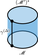
(c) A source $J=(\mathscr{M}^{\prime})^{*}\cdot\gamma^{(\Delta)}\cdot\mathscr{M}$ specifying conditions on a boundary manifold with pieces $\mathscr{M}$ and $(\mathscr{M}^{\prime})^{*}$ joined by a geodesic $\gamma^{(\Delta)}$. The length $\ell$ of the geodesic is to be integrated over with an extra weight $e^{-\Delta\ell}$.

Figure 1: Possible examples of sources $J\in\mathcal{J}$ (black) for the gravitational path integral. In each panel, a possible bulk configuration that might appear in the path integral $\zeta(J)$ is illustrated in blue.

If we do assume that $\zeta$ takes the form of an integral 2, then one example of a source $J\in\mathcal{J}$ is boundary conditions on a boundary manifold of the bulk spacetime. We will use $J=\mathscr{M}$ in the following discussion to refer to both the boundary manifold and the data on this manifold describing the boundary conditions satisfied by the bulk fields. For example, $\mathscr{M}$ it might specify the boundary configurations that fields such as the metric must asymptotically approach. In fig. 1(a), we illustrate a one-dimensional circular boundary manifold $\mathscr{M}$ on which boundary conditions are specified for a two-dimensional bulk theory. The boundary condition specified by such a source can in general be nontrivial and can be engineered to create excitations that propagate into the bulk. In particular, as illustrated in fig. 1(b), one can insert localized sources — in the conventional (A)dS/CFT sense of the word — on the boundary manifold $\mathscr{M}$ which produces excitations of bulk matter fields. In simple theories, such as two-dimensional topological models Marolf:2020xie or JT gravity, the matter excitations might be modelled simply as worldlines in the bulk emanating from defects on the boundary manifold.

The boundary manifold need not be connected. For example, a source

$$\mathscr{M}\sqcup\mathscr{M}^{\prime}\in\mathcal{J}$$ (3)

would specify boundary conditions on the disjoint union of two boundary manifolds $\mathscr{M}$ and $\mathscr{M}^{\prime}$. The path integral 2 can then include bulk spacetimes with arbitrary connections between the mutually disconnected pieces of the boundary manifold. Thus, generically,

$$\zeta(\mathscr{M}\sqcup\mathscr{M}^{\prime}) \neq\zeta(\mathscr{M})\,\zeta(\mathscr{M}^{\prime})\;.$$ (4)

We also allow the data on the boundary manifold to have nonlocal correlations. We can define, for example, a new source as the superposition of $d$-many sources of the kind 3,

$$\sum_{i=1}^{d}\mathscr{M}^{(i)}\sqcup\mathscr{M}^{\prime(i)}\in\mathcal{J}\;.$$ (5)

This formal sum is defined as the instruction to evaluate the path integral for each term individually and add the results together:

$$\zeta\left(\sum_{i=1}^{d}\mathscr{M}^{(i)}\sqcup\mathscr{M}^{\prime(i)}\right) =\sum_{i=1}^{d}\zeta\left(\mathscr{M}^{(i)}\sqcup\mathscr{M}^{\prime(i)}\right)\;.$$ (6)

So far, we have described examples where sources supply data on boundary manifolds. More generally, a source can specify the existence and properties of other objects in bulk configurations to be included in the path integral 2. An example of this is illustrated in fig. 1(c). Here, a source which we will write as $J=(\mathscr{M}^{\prime})^{*}\cdot\gamma\cdot\mathscr{M}$ includes not only a boundary manifold, given by pieces $\mathscr{M}$ and $(\mathscr{M}^{\prime})^{*}$, but also a worldline $\gamma$ in the bulk that is required to connect prescribed points on the boundary pieces. (The $*$ operation will be described in section 2.2 and is used here only to match later notation; the reader can safely regard $(\mathscr{M}^{\prime})^{*}$ here as an arbitrary boundary manifold.) The source might further specify that the worldline must be a geodesic, fix a prescribed length $\ell$ of the geodesic, or provide instructions to integrate over $\ell$ with some extra weight, say $e^{-\Delta\,\ell}$. The path integral 2 will then be restricted to configurations possessing the prescribed geodesic and satisfying the prescribed boundary conditions on the boundary manifold.

2.2 The commutative $*$-algebra $\mathcal{J}$ of sources and properties of the path integral $\zeta$

We will now proceed with an abstract discussion of the properties we require of $\mathcal{J}$ and $\zeta$. These properties will serve as the definition of a set $\mathcal{J}$ of sources and a function $\zeta:\mathcal{J}\to\mathbb{C}$ which we will call a gravitational path integral, irrespective of whether $\zeta$ truly comes from an integral 2 over bulk field configurations. Since this discussion will be quite abstract, the reader may find it helpful to keep eq. 2 and the examples of sources $J\in\mathcal{J}$ discussed in section 2.1 in mind.

At the outset, $\mathcal{J}$ is just a set of elements, each of which we call a source. Below, we will describe in turn each additional structure that we require $\mathcal{J}$ to have. At each step, we will also describe relevant properties required of the path integral with respect to this structure.

Firstly, we require $\mathcal{J}$ to be a vector space, typically of infinite dimension, over $\mathbb{C}$. That is, given any two sources $J,J^{\prime}\in\mathcal{J}$ and scalars $c,c^{\prime}\in\mathbb{C}$, we also include the formal linear combination

$$cJ+c^{\prime}J^{\prime}\in\mathcal{J}\;.$$ (7)

(Otherwise, we simply redefine $\mathcal{J}$ to include all such linear combinations.) By an abuse of notation, we will denote the additive identity in $\mathcal{J}$ with the same symbol $0$ as in $\mathbb{C}$. We will require the path integral $\zeta$ to act linearly, such that

$$\zeta(cJ+c^{\prime}J^{\prime}) =c\,\zeta(J)+c^{\prime}\,\zeta(J^{\prime})\;.$$ (8)

Conceptually, this relation defines what it means to take a formal linear combination of sources.

We further require $\mathcal{J}$ to have a multiplication operation

$$\sqcup:\mathcal{J}\times\mathcal{J} \to\mathcal{J}\;, J_{1},J_{2} \mapsto J_{1}\sqcup J_{2}\;,$$ (9)

which is monoidal, distributive over addition, and commutative, thus giving $\mathcal{J}$ the structure of a commutative ring. We will denote the $\sqcup$-multiplicative identity as $\varnothing\in\mathcal{J}$. We will further require $\sqcup$ to be compatible with scalar multiplication by complex numbers $c\in\mathbb{C}$,

$$c\,(J\sqcup J^{\prime}) =(cJ)\sqcup J^{\prime}=J\sqcup(c\,J^{\prime})\;.$$ (10)

Because $\mathcal{J}$ is a vector space and a commutative ring with compatible ring and scalar multiplication, it is a commutative algebra.

The symbols chosen above are purposely suggestive. In particular, suppose that $J$ and $J^{\prime}$ specify certain conditions on objects found in bulk configurations (e.g. boundary conditions on boundary manifolds). Then $J\sqcup J^{\prime}$ is to be interpreted as a source specifying those conditions on the disjoint union of the respective objects.

With respect to the path integral $\zeta$, let us remark firstly that implicit from the commutativity of $\sqcup$-multiplication is the requirement for $\zeta$ to be invariant,

$$\zeta(J\sqcup J^{\prime}) =\zeta(J^{\prime}\sqcup J)\;,$$ (11)

under the permutation of sources $J,J^{\prime}\in\mathcal{J}$. A second remark is that we do not require $\zeta$ to factorize between sources. That is, generically,

$$\zeta(J\sqcup J^{\prime}) \neq\zeta(J)\,\zeta(J^{\prime})\;.$$ (12)

This is because, if $\zeta(J\sqcup J^{\prime})$ is a literal path integral 2 that includes a sum over different spacetime geometries, then it is natural to allow arbitrary topologies in the sum, including those that connect the objects (e.g. boundary manifolds) in $J$ and $J^{\prime}$. Due to the generic lack of factorization, the path integral $\zeta$ is not necessarily an algebra homomorphism.

The final structure that we require $\mathcal{J}$ to have is an involution and automorphism $*$ satisfying

$$(J^{*})^{*} =J\;, (J+J^{\prime})^{*} =J^{*}+(J^{\prime})^{*}\;, (J\sqcup J^{\prime})^{*} =J^{*}\sqcup(J^{\prime})^{*}\;, \varnothing^{*} =\varnothing\;.$$ (13)

This gives $\mathcal{J}$ the structure of a commutative $*$-ring. We further require $*$ to be compatible with scalar multiplication,

$$(c\,J)^{*} =c^{*}J^{*}\;,$$ (14)

where we have denoted complex conjugation in $\mathbb{C}$ by $*$ as well. Thus, $\mathcal{J}$ is a commutative $*$-algebra.

The interpretation of $*$ is a complex conjugation and orientation- or time-reversal of sources. We require the path integral $\zeta$ to commute with $*$,

$$\zeta(J^{*}) =\zeta(J)^{*}\;.$$ (15)

Additionally, we require $\zeta$ to be reflection-positive, meaning

$$\zeta(J^{*}\sqcup J) \geq 0$$ (16)

is real and non-negative. We can therefore use $\zeta$ to define a positive semi-definite Hermitian form on $\mathcal{J}$:

$$\innerproduct{J^{\prime}}{J} =\zeta((J^{\prime})^{*}\sqcup J)\;.$$ (17)

In summary, the set $\mathcal{J}$ of sources is a commutative $*$-algebra. The path integral $\zeta:\mathcal{J}\to\mathbb{C}$ is almost a $*$-homomorphism, except it might fail to factorize, as expressed by the generic inequality 12. Additionally, $\zeta$ is required to be reflection-positive 16, thus equipping $\mathcal{J}$ with a positive semi-definite Hermitian form 17. These properties (together with a reflection-positivity condition generalizing eq. 16 to be specified in section 3.2) can be taken to be the definitions of a general set $\mathcal{J}$ of sources and a gravitational path integral $\zeta$.

2.3 The baby universe sector $\mathcal{H}_{\emptyset}$ of the gravitational Hilbert space

States of a quantum theory can be obtained from slicing the path integral. In this subsection, we will construct a Hilbert space $\mathcal{H}_{\emptyset}$ of states obtained from slicing the gravitational path integral in a way that avoids cutting sources, as illustrated in fig. 2. In particular, the bulk spacetime slices do not have spatial boundaries where boundary conditions are imposed by sources. The Hilbert space $\mathcal{H}_{\emptyset}$ therefore describes arbitrarily many closed universes, whose topology and local fields vary across configurations in the path integral, without being directly constrained by sources. We will loosely refer to such universes as baby universes.

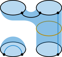
Figure 2: Slicing (orange) the gravitational path integral while avoiding cutting sources (black) gives a state in the baby universe Hilbert space.

In section 2.2, we defined the set $\mathcal{J}$ of sources to be a commutative $*$-algebra and therefore a vector space. We also required the path integral $\zeta:\mathcal{J}\to\mathbb{C}$ to be reflection-positive 16, such that it can be used in eq. 17 to define a positive semi-definite Hermitian form $\innerproduct{\bullet}{\bullet}$ on $\mathcal{J}$. We can therefore build a Hilbert space $\mathcal{H}_{\emptyset}$ from $\mathcal{J}$ as follows. First, we quotient $\mathcal{J}$ by null vectors. In particular, we define the subspace $\mathcal{N}\subset\mathcal{J}$ of null vectors to be the kernel of $\innerproduct{\bullet}{\bullet}$, meaning

$$\mathcal{N} =\left\{J\in\mathcal{J}:\innerproduct{J^{\prime}}{J}=0\quad\forall J^{\prime}\in\mathcal{J}\right\}\;.$$ (18)

We then consider the quotient $\mathcal{J}/\mathcal{N}$ which is a pre-Hilbert space on which $\innerproduct{\bullet}{\bullet}$ is a (positive-definite) inner product. Second, we take $\mathcal{H}_{\emptyset}$ to be the completion of $\mathcal{J}/\mathcal{N}$ with respect to the norm obtained from $\innerproduct{\bullet}{\bullet}$. We can construct this completion $\mathcal{H}_{\emptyset}$ as the set of equivalence classes of Cauchy sequences in $\mathcal{J}/\mathcal{N}$ where two sequences are equivalent if their difference converges to $0\in\mathcal{J}/\mathcal{N}$. Since $\mathcal{H}_{\emptyset}$ is a complete inner product space, it is a Hilbert space and, by construction, $\mathcal{J}/\mathcal{N}$ is a dense subspace of $\mathcal{H}_{\emptyset}$.

The states in $\mathcal{H}_{\emptyset}$ have the following interpretation. Consider a source $J\in\mathcal{J}$, which picks out an element $\ket{J}$ of $\mathcal{J}/\mathcal{N}\subset\mathcal{H}_{\emptyset}$. This is the state of baby universes prepared by the gravitational path integral from the source $J$. For example, $J$ might specify the boundary conditions at the spacetime boundary at “time-like $\infty$” or the Euclidean past. In particular, the special case where $J=\varnothing$ gives the no-boundary or Hartle-Hawking state $\ket{\varnothing}$. The baby universe Hilbert space $\mathcal{H}_{\emptyset}$ contains all such states prepared by sources $J\in\mathcal{J}$, as well as limits of these states, with two states identified as equal if their difference has vanishing norm under the inner product $\innerproduct{\bullet}{\bullet}$ determined by the path integral 17.

For each source $J\in\mathcal{J}$, we can also define an operator $Z(J)$ on $\mathcal{J}/\mathcal{N}$. In particular, for any $J^{\prime}\in\mathcal{J}$, we define

$$Z(J)\ket{J^{\prime}} =\ket{J\sqcup J^{\prime}}\;.$$ (19)

This is a well-defined operator on equivalence classes under the quotient $\mathcal{J}/\mathcal{N}$ — for any $N\in\mathcal{N}$, we also have $J\sqcup N\in\mathcal{N}$. From the definition 17 of the inner product, we see that matrix elements of the adjoint is given by

$$\matrixelement{J^{\prime}}{Z(J)^{\dagger}}{J^{\prime\prime}} =\matrixelement{J^{\prime}}{Z(J^{*})}{J^{\prime\prime}}\;.$$ (20)

Moreover, because of the commutativity of $\sqcup$-multiplication, we find that any two such operators commute,

$$Z(J)\,Z(J^{\prime}) =Z(J^{\prime})\,Z(J)\;.$$ (21)

We have thus far described these operators on $\mathcal{J}/\mathcal{N}$. Because these operators can have unbounded norm, it remains a nontrivial question whether they have extensions to domains in $\mathcal{H}_{\emptyset}$ on which they satisfy $Z(J)^{\dagger}=Z(J^{*})$ and eq. 21. The answer can be model-dependent.

We will simply proceed as in refs. Marolf:2020xie ; Marolf:2024jze , assuming that real bounded functions of

$$\real Z(J) =\frac{Z(J)+Z(J^{*})}{2}\;, \imaginary Z(J) =\frac{Z(J)-Z(J^{*})}{2i}$$ (22)

define operators with unique self-adjoint extensions to $\mathcal{H}_{\emptyset}$ which commute with each other and between all $J\in\mathcal{J}$. We can therefore simultaneously diagonalize $Z(J)$ for all $J\in\mathcal{J}$. Denoting the joint spectrum of all $Z(J)$ by $\mathcal{A}$, the baby universe Hilbert space $\mathcal{H}_{\emptyset}$ decomposes into a direct sum or integral,

$$\mathcal{H}_{\emptyset} =\int_{\mathcal{A}}^{\oplus}\differential{\alpha}\mathcal{H}_{\emptyset}^{\alpha}\;,$$ (23)

into superselection sectors $\mathcal{H}_{\emptyset}^{\alpha}$, or “$\alpha$-sectors” for brevity, in which the operators $Z(J)$ take definite eigenvalues $Z_{\alpha}(J)$. In fact, each baby universe $\alpha$-sector $\mathcal{H}_{\emptyset}^{\alpha}$ is one dimensional. In particular, it is spanned by a single state $\ket{\alpha}$ — a so-called “$\alpha$-state” Coleman:1988cy ; Giddings:1988cx — uniquely determined (up to scalar multiplication) by the values of the inner product

$$\innerproduct{\alpha}{J} =\matrixelement{\alpha}{Z(J)}{\varnothing}=Z_{\alpha}(J)\innerproduct{\alpha}{\varnothing}$$ (24)

with states $\ket{J}$ spanning the dense subspace $\mathcal{J}/\mathcal{N}\subset\mathcal{H}_{\emptyset}$. In particular, the linear combination $\innerproduct{\varnothing}{\alpha}^{\prime}\ket{\alpha}-\innerproduct{\varnothing}{\alpha}\ket{\alpha}^{\prime}$ of any two $\ket{\alpha},\ket{\alpha}^{\prime}\in\mathcal{H}_{\emptyset}^{\alpha}$ has vanishing inner product with all $\ket{J}$ by eq. 24 and must therefore be identified with $0$.

Since $\alpha$-states form an orthonormal basis spanning $\mathcal{H}_{\emptyset}$, we can express the path integral $\zeta$ as an ensemble-average over $\alpha$-sectors,

$$\zeta(J) =\int_{\mathcal{A}}\differential{\alpha}\absolutevalue{\innerproduct{\alpha}{\varnothing}}^{2}\,\zeta_{\alpha}(J)\;,$$ (25)

where

$$\zeta_{\alpha}(J) \coloneqq\frac{\matrixelement{\alpha}{Z(J)}{\alpha}}{\innerproduct{\alpha}{\alpha}}=Z_{\alpha}(J)\;,$$ (26)

and we have chosen to normalize $\ket{\alpha}$ such that $\innerproduct{\alpha^{\prime}}{\alpha}$ is the $\delta$-function on $\mathcal{A}$ with measure $\differential{\alpha}$. As explained in refs. Marolf:2020xie ; Marolf:2024jze , each $\zeta_{\alpha}(J)$ is itself a path integral in the sense that it is equal to a limit of the original path integral $\zeta(J\sqcup J^{\alpha}_{\nu})$ with the insertion of extra sources $J^{\alpha}_{\nu}\in\mathcal{J}$ whose corresponding operators converge to

$$\lim_{\nu}Z(J^{\alpha}_{\nu}) =\frac{\outerproduct{\alpha}{\alpha}}{\absolutevalue{\innerproduct{\alpha}{\varnothing}}^{2}}\;.$$ (27)

In contrast to eq. 12, these path integrals over individual $\alpha$-sectors do factorize:

$$Z_{\alpha}(J\sqcup J^{\prime}) =Z_{\alpha}(J)\,Z_{\alpha}(J^{\prime})\;.$$ (28)

Let us comment briefly on, e.g. holographic, contexts in which the sources $J\in\mathcal{J}$ specify objects, e.g. boundary manifolds, which host theories, e.g. CFTs, dual to the bulk gravitational theory. The partition function of a local dual theory must factorize as in eq. 28 where $J$ and $J^{\prime}$ specify mutually disconnected objects. The gravitational bulk dual of a single dual theory must correspond to an individual $\alpha$-sector, with a factorizing path integral $\zeta_{\alpha}$. The generically non-factorizing gravitational path integral $\zeta$ then corresponds to an ensemble average of the partition functions of dual theories.

3 Partial sources and the Hilbert spaces of states they prepare

In section 2, we described the set $\mathcal{J}$ of sources which serve as inputs to the path integral $\zeta:\mathcal{J}\to\mathbb{C}$. Each such source $J\in\mathcal{J}$ is completely specified in the sense that it contains the full input needed for the path integral to output a complex number $\zeta(J)$. A goal of this section is to describe objects which we will call partial sources. A partial source $J_{C}$ is characterized by the property that it produces a complete source, written as $(J_{C}^{\prime}|J_{C})\in\mathcal{J}$, once it is glued across what we will call a cut $C$ with another, compatible partial source $(J_{C}^{\prime})^{*}$.

The outline of this section is much like that of section 2. In section 3.1, we will first provide some possible examples of partial sources. The reader may find it helpful to bear these in mind as we proceed with a more abstract discussion in section 3.2. There, we describe the general defining properties we demand of the set $\mathcal{C}$ of cuts $C$ and the set $\mathcal{J}_{C}$ of partial sources $J_{C}$ associated with each cut $C$. Finally, in section 3.3, we will use $\mathcal{J}_{C}$ to construct a Hilbert space $\mathcal{H}_{C}$ of states prepared by partial sources $J_{C}\in\mathcal{J}_{C}$. Notably, the $\alpha$-sectors $\mathcal{H}_{C}^{\alpha}$ of $\mathcal{H}_{C}$ need not be one-dimensional.

3.1 Possible examples of cuts $C\in\mathcal{C}$ and partial sources $J_{C}\in\mathcal{J}_{C}$

As with $\mathcal{J}$, the set $\mathcal{C}$ of cuts $C$ and the set $\mathcal{J}_{C}$ of partial sources $J_{C}$ will be theory-dependent. We will now give some illustrative examples of these objects, which may or may not be in a given theory.

(a) A partial boundary manifold $J_{\Sigma}=\mathscr{N}_{\Sigma}$ with boundary $C=\Sigma$.

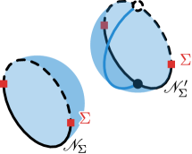
(b) A partial boundary manifold $J_{C}^{(\ref{fig:psourceotimes1})}=\mathscr{N}_{\Sigma}\otimes\mathscr{N}_{\Sigma}^{\prime}$ with boundary $C=\Sigma\otimes\Sigma$. (The superscript on $J_{C}^{(\ref{fig:psourceotimes1})}$ is introduced for disambiguation with fig. 3(c).)

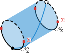
(c) A partial boundary manifold $J_{C}^{(\ref{fig:psourceotimes2})}=\mathscr{N}_{\Sigma}^{\prime}\otimes\mathscr{N}_{\Sigma}$ with boundary $C=\Sigma\otimes\Sigma$. The cut $C$ here is the same as in fig. 3(b). However, $\mathscr{N}_{\Sigma}\neq\mathscr{N}_{\Sigma}^{\prime}$ so $J_{C}^{(\ref{fig:psourceotimes1})}\neq{}J_{C}^{(\ref{fig:psourceotimes2})}$ and $(J_{C}^{\prime}|J_{C}^{(\ref{fig:psourceotimes1})})\neq{}(J_{C}^{\prime}|J_{C}^{(\ref{fig:psourceotimes2})})$ for the same $J_{C}^{\prime}$ as in fig. 3(b).

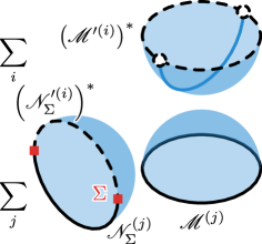
(d) A formal linear combination $J_{\Sigma}=\sum_{j=1}^{d}\mathscr{M}^{(j)}\sqcup\mathscr{N}_{\Sigma}^{(j)}$ of partial boundary manifolds where each $\mathscr{N}_{\Sigma}^{(j)}$ has boundary $C=\Sigma$.

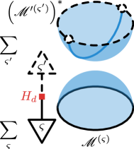
(e) A formal linear combination $J_{d}=\sum_{\varsigma=1}^{d}\mathscr{M}^{(\varsigma)}\ket{\varsigma}$ built from states $\ket{\varsigma}$, spanning a nongravitational Hilbert space $C=H_{d}$, and boundary manifolds $\mathscr{M}^{(\varsigma)}\in\mathcal{J}$, playing the role of scalars.

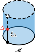
(f) A partial source $J_{\Delta}=\xi_{\Delta}\cdot\mathscr{M}$, obtained from cutting the geodesic in fig. 1(c). The value of $\Delta$ in this example is specified by the cut $C$.

Figure 3: Possible examples of cuts $C\in\mathcal{C}$ (red) and partial sources $J_{C}\in\mathcal{J}_{C}$ (solid black). In each panel, the complete source $(J_{C}^{\prime}|J_{C})\in\mathcal{J}$ obtained from gluing with another partial source $(J_{C}^{\prime})^{*}$ (dashed black) is also shown. A possible bulk configuration that might appear in the path integral $\zeta(J_{C}^{\prime}|J_{C})$ is illustrated in blue.

The perhaps most straightforward example of a partial source is the specification of boundary conditions for bulk fields on a part $J_{C}=\mathscr{N}_{\Sigma}$ of a boundary manifold. This is illustrated in fig. 3(a). The partial boundary manifold $\mathscr{N}_{\Sigma}$ is a manifold itself with a boundary $C=\Sigma$. (We will use $\mathscr{N}_{\Sigma}$ and $\Sigma$ to refer to both the partial boundary manifold and its boundary, as well as data specified there.)

If we have two such partial sources $\mathscr{N}_{\Sigma}$ and $\mathscr{N}_{\Sigma}^{\prime}$ associated with the same cut $\Sigma$, then we can form a complete source $(\mathscr{N}_{\Sigma}^{\prime}|\mathscr{N}_{\Sigma})\in\mathcal{J}$ as follows. Firstly, we apply a complex conjugation and time- or orientation-reversal transformation $\mathscr{N}_{\Sigma}^{\prime}\mapsto(\mathscr{N}_{\Sigma}^{\prime})^{*}$. We then glue each point $p\in\Sigma=\partial\mathscr{N}$ to its image $p^{*}$ on the boundary $\Sigma^{*}=\partial(\mathscr{N}_{\Sigma}^{\prime})^{*}$ of the partial boundary manifold $(\mathscr{N}_{\Sigma}^{\prime})^{*}$, thus producing a complete source $(\mathscr{N}_{\Sigma}^{\prime}|\mathscr{N}_{\Sigma})\in\mathcal{J}$ specifying boundary conditions on a boundary manifold itself without boundary. Let us emphasize that the points in $\Sigma$ are marked by unique labels, such that each point $p\in\Sigma$ corresponds and is glued to a unique point $p^{*}\in\Sigma^{*}$. The gluing is therefore unique, even if $\Sigma$ possesses isometries.

In general, a cut $C$ provides specifications to ensure that two partial sources $J_{C},J_{C}^{\prime}\in\mathcal{J}_{C}$ associated with the same cut can be joined to produce a source $(J_{C}|J_{C}^{\prime})\in\mathcal{J}$. In the current example, if $\mathscr{N}_{\Sigma},\mathscr{N}_{\Sigma}^{\prime}\in\mathcal{J}_{\Sigma}$ specify local background fields (conventionally called sources of the boundary theory in (A)dS/CFT) which parametrize boundary conditions for bulk fields, then $C=\Sigma$ might specify the values these fields on the cut, to ensure continuity in $(\mathscr{N}_{\Sigma}|\mathscr{N}_{\Sigma}^{\prime})\in\mathcal{J}$. Higher derivatives would also be needed to meet stronger smoothness requirements that might be required for sources in $\mathcal{J}$.

Let us comment briefly on the holographic interpretation of the above construction, where we suppose the dual boundary theories are non-gravitational QFTs. In each QFT, the overlap of two states, prepared by QFT path integrals on the backgrounds $\mathscr{N}_{\Sigma}$ and $\mathscr{N}_{\Sigma}^{\prime}$, is computed by a partition function over the background $(\mathscr{N}_{\Sigma}|\mathscr{N}_{\Sigma}^{\prime})$. Ensuring that $(\mathscr{N}_{\Sigma})^{*}$ and $\mathscr{N}_{\Sigma}^{\prime}$ can be glued together is equivalent to ensuring that the prepared states belong to the same Hilbert space. Thus, $C=\Sigma$ in this holographic context can be interpreted as specifying the QFT Hilbert space for each boundary theory (in the ensemble), which can depend on the value of background fields, e.g. the metric, near the cut as described in the previous paragraph.

As for boundary manifolds, a partial boundary manifold need not be connected. Given a source $\mathscr{M}\in\mathcal{J}$ specifying boundary conditions on a boundary manifold $\mathscr{M}$ and a partial source $\mathscr{N}_{\Sigma}\in\mathcal{J}_{\Sigma}$ specifying boundary conditions on a partial boundary manifold $\mathscr{N}_{\Sigma}$, we can also consider a partial source

$$\mathscr{M}\sqcup\mathscr{N}_{\Sigma}\in\mathcal{J}_{\Sigma}\;,$$ (29)

specifying the boundary conditions on the disjoint union of $\mathscr{M}$ and $\mathscr{N}_{\Sigma}$. Given another partial source $\mathscr{N}_{\Sigma^{\prime}}\in\mathcal{J}_{\Sigma^{\prime}}$, we can also consider a partial source

$$\mathscr{N}_{\Sigma}\otimes\mathscr{N}_{\Sigma^{\prime}}\in\mathcal{J}_{\Sigma\otimes\Sigma^{\prime}}\;,$$ (30)

with a cut $\Sigma\otimes\Sigma^{\prime}$. Here, $\otimes$ can be thought of as disjoint union with the understanding that points in $\Sigma\otimes\Sigma^{\prime}$ are marked by unique labels. Even if $\Sigma=\Sigma^{\prime}$ so that $\Sigma\otimes\Sigma^{\prime}=\Sigma^{\prime}\otimes\Sigma$, we still have $\mathscr{N}_{\Sigma}\otimes\mathscr{N}_{\Sigma}^{\prime}\neq\mathscr{N}_{\Sigma}^{\prime}\otimes\mathscr{N}_{\Sigma}$ for $\mathscr{N}_{\Sigma}\neq\mathscr{N}_{\Sigma}^{\prime}$ in $\mathcal{J}_{\Sigma}$ — see figs. 3(b) and 3(c). The choice of symbol $\otimes$ is purposely evocative of a tensor product, as we will explain in our abstract discussion of partial sources in section 3.2. In particular, the gluing of partial sources described above is reminiscent of tensor contraction, which we shall denote like

$$(\mathscr{N}_{\Sigma}|\mathscr{N}_{\Sigma}^{\prime}) =(\mathscr{N}_{\mathchoice{\leavevmode\hbox to5.71pt{\vbox to4.78pt{\text{[drawing]}}}}{\leavevmode\hbox to5.71pt{\vbox to4.78pt{\text{[drawing]}}}}{\leavevmode\hbox to3.54pt{\vbox to3.35pt{\text{[drawing]}}}}{\leavevmode\hbox to2.53pt{\vbox to2.39pt{\text{[drawing]}}}}})^{*}\otimes\mathscr{N}_{\mathchoice{\leavevmode\hbox to5.71pt{\vbox to4.78pt{\text{[drawing]}}}}{\leavevmode\hbox to5.71pt{\vbox to4.78pt{\text{[drawing]}}}}{\leavevmode\hbox to3.54pt{\vbox to3.35pt{\text{[drawing]}}}}{\leavevmode\hbox to2.53pt{\vbox to2.39pt{\text{[drawing]}}}}}^{\prime}\in\mathcal{J}\;.\leavevmode\hbox to0pt{\vbox to0pt{\text{[drawing]}}} \scriptstyle\Sigma \scriptstyle\Sigma$$ (31)

As for boundary manifolds, we can also consider superpositions of partial boundary manifolds. To prepare a convenient segue in our discussion, let us consider superpositions of $d$-many partial boundary manifolds of the kind 29:

$$J_{\Sigma} =\sum_{j=1}^{d}\mathscr{M}^{(j)}\sqcup\mathscr{N}_{\Sigma}^{(j)}\in\mathcal{J}_{\Sigma}\;, J_{\Sigma}^{\prime} =\sum_{i=1}^{d}\mathscr{M}^{\prime(i)}\sqcup\mathscr{N}_{\Sigma}^{\prime(i)}\in\mathcal{J}_{\Sigma}\;.$$ (32)

See fig. 3(d). Again, we can define $(\bullet|\bullet)$ to mean taking the $*$-conjugation of the first argument and gluing to the second argument, giving a Hermitian form

$$(J_{\Sigma}^{\prime}|J_{\Sigma}) =\sum_{i,j=1}^{d}(\mathscr{M}^{\prime(i)})^{*}\sqcup\mathscr{M}^{(j)}\sqcup(\mathscr{N}_{\Sigma}^{\prime(i)}|\mathscr{N}_{\Sigma}^{(j)})\in\mathcal{J}\;.$$ (33)

The above formulas suggest a natural generalization to other possible types of partial sources that the theory might allow. In particular, let the cut $C=H_{d}$ be any $d$-dimensional Hilbert space of a non-gravitational system, spanned by states $\ket{\varsigma}$. (From here on, when it appears in a subscript, we will abreviate $H_{d}$ as simply $d$.) We can then consider the set of formal linear combinations

$$\mathcal{J}_{d}=\left\{\sum_{\varsigma=1}^{d}J^{(\varsigma)}\ket{\varsigma}:J^{(\varsigma)}\in\mathcal{J}\right\}\;.$$ (34)

Some examples of these partial sources $J_{d}\in\mathcal{J}_{d}$ are illustrated in fig. 3(e), where each $J^{(\varsigma)}$ is a boundary manifold $\mathscr{M}^{(\varsigma)}$. With the obvious replacements in eq. 33, for any two $J_{d},J_{d}^{\prime}\in\mathcal{J}_{d}$, we can define the Hermitian form

$$(J_{d}^{\prime}|J_{d}) =\sum_{\varsigma,\varsigma^{\prime}=1}^{d}(J^{\prime(\varsigma^{\prime})})^{*}\sqcup J^{(\varsigma)}\innerproduct{\varsigma^{\prime}}{\varsigma}\in\mathcal{J}\;.$$ (35)

This can again be viewed as taking a $*$-conjugation of the first argument and gluing its cut to the cut of second argument, if we define

$$\ket{\varsigma}^{*} =\bra{\varsigma}$$ (36)

and the gluing to mean

$$\bra{\varsigma^{\prime}}\otimes\ket{\varsigma} \mapsto\mathchoice{\leavevmode\hbox to13.1pt{\vbox to10.52pt{\text{[drawing]}}}}{\leavevmode\hbox to13.1pt{\vbox to10.02pt{\text{[drawing]}}}}{\leavevmode\hbox to11.39pt{\vbox to7.55pt{\text{[drawing]}}}}{\leavevmode\hbox to10.87pt{\vbox to5.5pt{\text{[drawing]}}}}\otimes\mathchoice{\leavevmode\hbox to10.3pt{\vbox to10pt{\text{[drawing]}}}}{\leavevmode\hbox to10.3pt{\vbox to10pt{\text{[drawing]}}}}{\leavevmode\hbox to8.69pt{\vbox to7pt{\text{[drawing]}}}}{\leavevmode\hbox to8.17pt{\vbox to5pt{\text{[drawing]}}}}=\innerproduct{\varsigma^{\prime}}{\varsigma}\;.\leavevmode\hbox to0pt{\vbox to0pt{\text{[drawing]}}} \bra{\varsigma^{\prime}} \ket{\varsigma}$$ (37)

For simplicity, when we continue our discussion of this example in section 5.2.2, we will choose the states $\ket{\varsigma}$ to be orthonormal:

$$\innerproduct{\varsigma^{\prime}}{\varsigma} =\delta_{\varsigma^{\prime}\varsigma}\;.$$ (38)

More examples of partial sources might arise from cutting geometric objects other than boundary manifolds specified by complete sources found in $\mathcal{J}$. For example, as illustrated in fig. 3(f), if $\mathcal{J}$ contains sources of the form $(\mathscr{M}^{\prime})^{*}\cdot\gamma\cdot\mathscr{M}$ illustrated in fig. 1(c), we can cut a bulk worldline $\gamma$ to obtain a partial source, which we write as $\xi\cdot\mathcal{M}$, with a partial worldline $\xi$. By definition, a partial worldline $\xi$ with the same cut $C$ can be glued to its $*$-conjugate to give a full worldline $\gamma$ that would appear in a complete source, say

$$(\xi\cdot\mathscr{M}^{\prime}|\xi\cdot\mathscr{M})=(\mathscr{M}^{\prime})^{*}\cdot\gamma\cdot\mathscr{M}\in\mathcal{J}\;.$$ (39)

In the example with a geodesic $\gamma^{(\Delta)}$ whose length $\ell$ is to be integrated over with weight $e^{-\Delta\,\ell}$, the cut $C$ would in particular specify the value of $\Delta$ and perhaps the flavour $\sigma$ of the worldline if there exist multiple flavours. When $C$ appears in a subscript in this case, we will write it simply as $\Delta$ or $\sigma$ as appropriate — e.g., we might use $\mathcal{J}_{\Delta}$ or $\mathcal{J}_{\sigma}$ to denote the set of partial sources with partial worldlines terminating at a cut corresponding to a value of $\Delta$ or a worldline flavour $\sigma$.

3.2 The monoid $\mathcal{C}$ of cuts $C$ and the $\mathcal{J}$-modules $\mathcal{J}_{C}$ of partial sources

We will now proceed with an abstract discussion of the properties we require of $\mathcal{C}$ and $\mathcal{J}_{C}$. These properties can be taken to be our general definition for a set $\mathcal{C}$ of cuts $C$ and the set $\mathcal{J}_{C}$ of partial sources associated with a cut $C$, irrespective of how they are concretely realized in the examples discussed in section 3.1. The reader may nonetheless find it helpful to bear those examples in mind to conceptually motivate the abstract structures we will discuss.

At the outset, $\mathcal{C}$ is just a set of elements, each of which we call a cut. For each cut $C\in\mathcal{C}$, $\mathcal{J}_{C}$ is itself a set of elements, each of which we will call a partial source associated with the cut $C$. Below, we will describe in turn each additional structure that we require $\mathcal{J}_{C}$ and $\mathcal{C}$ to have.

Firstly, we require each $\mathcal{J}_{C}$ to be a $\mathcal{J}$-module. That is, $\mathcal{J}_{C}$ is equipped with addition $+$ and scalar multiplication $\sqcup$ operations, where elements of the ring $\mathcal{J}$ play the role of scalars. For all $J,J^{\prime}\in\mathcal{J}$ and $J_{C},J_{C}^{\prime}\in\mathcal{J}_{C}$, these operations satisfy

$$J\sqcup(J_{C}+J_{C}^{\prime}) =J\sqcup J_{C}+J\sqcup J_{C}^{\prime}\;,$$ (40)

$$(J+J^{\prime})\sqcup J_{C} =J\sqcup J_{C}+J^{\prime}\sqcup J_{C}\;,$$ (41)

$$(J\sqcup J^{\prime})\sqcup J_{C} =J\sqcup(J^{\prime}\sqcup J_{C})\;,$$ (42)

$$\varnothing\sqcup J_{C} =J_{C}\;.$$ (43)

(Because the ring $\mathcal{J}$ is commutative, left $\mathcal{J}$-modules are the same as right $\mathcal{J}$-modules.) Again, by an abuse of notation, we will denote the additive identity in $\mathcal{J}_{C}$ with the same symbol $0$ as in $\mathbb{C}$.

Next, we require $\mathcal{C}$ to have an associative (but not necessarily commutative) multiplication operation, which we denote as

$$\otimes:\mathcal{C}\times\mathcal{C} \to\mathcal{C}\;, C,C^{\prime} \mapsto C\otimes C^{\prime}\;.$$ (44)

This gives $\mathcal{C}$ the structure of a semigroup. We will use the same symbol $\otimes$ to denote the tensor product on vector spaces or, more generally, modules. In particular,

$$\otimes:\mathcal{J}_{C}\times\mathcal{J}_{C^{\prime}} \to\mathcal{J}_{C}\otimes\mathcal{J}_{C^{\prime}}\;, J_{C},J_{C^{\prime}} \mapsto J_{C}\otimes J_{C^{\prime}}\;,$$ (45)

is the tensor product on the $\mathcal{J}$-modules $\mathcal{J}_{C},\mathcal{J}_{C^{\prime}}$ of partial sources. The relation to the multiplication 44 of cuts is that we require $\mathcal{J}_{C}\otimes\mathcal{J}_{C^{\prime}}$ to be a submodule of $\mathcal{J}_{C\otimes C^{\prime}}$. It may be the case that $\mathcal{J}_{C\otimes{}C^{\prime}}$ contains more partial sources, e.g. connecting the two pieces $C$ and $C^{\prime}$ of the cut $C\otimes C^{\prime}$, so $\mathcal{J}_{C}\otimes\mathcal{J}_{C^{\prime}}$ might be a proper submodule.

We require $\mathcal{C}$ to have a (left and right) $\otimes$-multiplicative identity element $\emptyset\in\mathcal{C}$. Thus, $\mathcal{C}$ is a monoid. For this trivial cut $\emptyset$, we set

$$\mathcal{J}_{\emptyset}=\mathcal{J}\;,$$ (46)

with $\mathcal{J}$ considered as a module over itself. Thus, complete sources are partial sources associated with the trivial cut $\emptyset$. For all $J\in\mathcal{J}$, $C\in\mathcal{C}$, and $J_{C}\in\mathcal{J}_{C}$, we in particular have

$$\mathcal{J}_{C}\otimes\mathcal{J}_{\emptyset} =\mathcal{J}_{\emptyset}\otimes\mathcal{J}_{C}=\mathcal{J}_{C}\;,$$ (47a)

$$J_{C}\otimes J =J\otimes J_{C}=J\sqcup J_{C}\;.$$ (47b)

The next structure we require $\mathcal{C}$ to have is an involution and automorphism $*$, i.e.,

$$(C^{*})^{*} =C\;, (C\otimes C^{\prime})^{*} =C^{*}\otimes(C^{\prime})^{*}\;, \emptyset^{*} =\emptyset$$ (48)

for all $C,C^{\prime}\in\mathcal{C}$. We will correspondingly require $\mathcal{J}_{C}$ and $\mathcal{J}_{C^{*}}$ to be related by an involution and homomorphism $*$, i.e.

$$(J_{C}^{*})^{*} =J_{C}\;, (J\sqcup J_{C}+J_{C}^{\prime})^{*} =J^{*}\sqcup J_{C}^{*}+(J_{C}^{\prime})^{*}\in\mathcal{J_{C^{*}}}\;, (J_{C}\otimes J_{C^{\prime}})^{*} =J_{C}^{*}\otimes J_{C^{\prime}}^{*}\;.$$ (49)

To glue together cuts of partial sources, we require a linear gluing operation which is analogous to tensor contraction,

$$\cup:\mathcal{J}_{C_{1}\otimes C\otimes C_{2}\otimes C^{*}\otimes C_{3}} \to\mathcal{J}_{C_{1}\otimes C_{2}\otimes C_{3}}\;, J_{C_{1}\otimes C\otimes C_{2}\otimes C^{*}\otimes C_{3}}\mapsto J_{C_{1}\otimes\mathchoice{\leavevmode\hbox to6.23pt{\vbox to4.78pt{\text{[drawing]}}}}{\leavevmode\hbox to6.23pt{\vbox to4.78pt{\text{[drawing]}}}}{\leavevmode\hbox to3.85pt{\vbox to3.35pt{\text{[drawing]}}}}{\leavevmode\hbox to2.75pt{\vbox to2.39pt{\text{[drawing]}}}}\otimes C_{2}\otimes\mathchoice{\leavevmode\hbox to6.23pt{\vbox to4.78pt{\text{[drawing]}}}}{\leavevmode\hbox to6.23pt{\vbox to4.78pt{\text{[drawing]}}}}{\leavevmode\hbox to3.85pt{\vbox to3.35pt{\text{[drawing]}}}}{\leavevmode\hbox to2.75pt{\vbox to2.39pt{\text{[drawing]}}}}^{*}\otimes C_{3}}\;.\leavevmode\hbox to0pt{\vbox to0pt{\text{[drawing]}}} \scriptstyle C \scriptstyle C$$ (50)

Naturally, we require gluing operations to commute with each other, with the $*$-involution of the partial source, and with taking the tensor product with another partial source. Additionally, we require gluing to distribute over products of cuts, meaning a gluing of $C=C^{\prime}\otimes{}C^{\prime\prime}$ to $C^{*}=(C^{\prime})^{*}\otimes{}(C^{\prime\prime})^{*}$ is equal to the gluing of $C^{\prime}$ to $(C^{\prime})^{*}$ and of $C^{\prime\prime}$ to $(C^{\prime\prime})^{*}$. Finally, we require any partial source whose cut has all its components glued to other cuts to commute in tensor products with other partial sources.

It will also be convenient for our later analysis in section 4 to introduce a swap operation, which is analogous to permuting tensor indices,

$$\operatorname{\leavevmode\hbox to10.52pt{\vbox to11.95pt{\text{[drawing]}}}}:\mathcal{J}_{C_{1}\otimes C\otimes C_{2}\otimes C^{\prime}\otimes C_{3}} \to\mathcal{J}_{C_{1}\otimes C^{\prime}\otimes C_{2}\otimes C\otimes C_{3}}\;, J_{C_{1}\otimes C\otimes C_{2}\otimes C^{\prime}\otimes C_{3}}\mapsto J_{C_{1}\otimes\mathchoice{\leavevmode\hbox to6.23pt{\vbox to4.78pt{\text{[drawing]}}}}{\leavevmode\hbox to6.23pt{\vbox to4.78pt{\text{[drawing]}}}}{\leavevmode\hbox to3.85pt{\vbox to3.35pt{\text{[drawing]}}}}{\leavevmode\hbox to2.75pt{\vbox to2.39pt{\text{[drawing]}}}}\otimes C_{2}\otimes\mathchoice{\leavevmode\hbox to6.23pt{\vbox to4.78pt{\text{[drawing]}}}}{\leavevmode\hbox to6.23pt{\vbox to4.78pt{\text{[drawing]}}}}{\leavevmode\hbox to3.85pt{\vbox to3.35pt{\text{[drawing]}}}}{\leavevmode\hbox to2.75pt{\vbox to2.39pt{\text{[drawing]}}}}^{\prime}\otimes C_{3}}\;.\leavevmode\hbox to0pt{\vbox to0pt{\text{[drawing]}}} \scriptstyle C \scriptstyle C$$ (51)

Like the gluing operation, we require the swap to commute with the $*$-involution of the partial source, commute with taking the tensor product with another partial source, and distribute over products of cuts. The rules we require for composing swaps with each other and with gluing are exactly those intuited from the “circuit diagram” built by successively attaching pieces of “wire” $\cup$ and $\operatorname{\leavevmode\hbox to10.52pt{\vbox to11.95pt{\text{[drawing]}}}}$, e.g.

$$=\vbox{\hbox{ \leavevmode\hbox to63.57pt{\vbox to27.6pt{\text{[drawing]}}} }}\;, =\vbox{\hbox{ \leavevmode\hbox to92.02pt{\vbox to16.21pt{\text{[drawing]}}} }}\;,$$ (52)

where we have used colours to emphasize that the wires on both sides of each equality connect the same cuts.

Using the $*$-involution and the gluing operation, we can construct a Hermitian form on each $\mathcal{J}_{C}$,

$$(\bullet|\bullet):\mathcal{J}_{C}\times\mathcal{J}_{C} \to\mathcal{J}\;, J_{C}^{\prime},J_{C} \mapsto(J_{C}^{\prime}|J_{C})=(J_{\mathchoice{\leavevmode\hbox to6.23pt{\vbox to4.78pt{\text{[drawing]}}}}{\leavevmode\hbox to6.23pt{\vbox to4.78pt{\text{[drawing]}}}}{\leavevmode\hbox to3.85pt{\vbox to3.35pt{\text{[drawing]}}}}{\leavevmode\hbox to2.75pt{\vbox to2.39pt{\text{[drawing]}}}}}^{\prime})^{*}\otimes J_{\mathchoice{\leavevmode\hbox to6.23pt{\vbox to4.78pt{\text{[drawing]}}}}{\leavevmode\hbox to6.23pt{\vbox to4.78pt{\text{[drawing]}}}}{\leavevmode\hbox to3.85pt{\vbox to3.35pt{\text{[drawing]}}}}{\leavevmode\hbox to2.75pt{\vbox to2.39pt{\text{[drawing]}}}}}\;.\leavevmode\hbox to0pt{\vbox to0pt{\text{[drawing]}}} \scriptstyle C \scriptstyle C$$ (53)

It follows from the properties of the gluing operation that $(\bullet|\bullet)$ is compatible with the tensor product $\otimes$, meaning

$$(J_{C}^{\prime}\otimes J_{C^{\prime}}^{\prime}|J_{C}\otimes J_{C^{\prime}}) =(J_{C}^{\prime}|J_{C})\sqcup(J_{C^{\prime}}^{\prime}|J_{C^{\prime}})\;.$$ (54)

For sources $J^{\prime},J\in\mathcal{J}=\mathcal{J}_{\emptyset}$, gluing acts trivially on the trivial cut $\emptyset$ and $\otimes$ reduces to $\sqcup$ by eq. 47, so we simply have

$$(J^{\prime}|J)=(J^{\prime})^{*}\sqcup J\;.$$ (55)

In addition to the properties of the path integral $\zeta$ laid out in section 2.2, we further require $\zeta$ to be reflection-positive with respect to partial sources. That is, for all $C\in\mathcal{C}$ and $J_{C}\in\mathcal{J}_{C}$,

$$\zeta(J_{C}|J_{C}) \geq 0\;.$$ (56)

This allows us to define a positive semi-definite Hermitian form on each $\mathcal{J}_{C}\ni J_{C}^{\prime},J_{C}$ as a vector space over $\mathbb{C}$:

$$\innerproduct{J_{C}^{\prime}}{J_{C}}=\zeta(J_{C}^{\prime}|J_{C})\;.$$ (57)

(Since $\mathcal{J}$ is a vector space over $\mathbb{C}$, so is $\mathcal{J}_{C}$.) Given eq. 55, note that eqs. 16 and 17 are special cases of eqs. 56 and 57.

In summary, the set $\mathcal{C}$ of cuts is a monoid and the set $\mathcal{J}_{C}$ of partial sources for each cut $C\in\mathbb{C}$ is a $\mathcal{J}$-module, such that the tensor product $\mathcal{J}_{C}\otimes\mathcal{J}_{C^{\prime}}$ is required to be a submodule of $\mathcal{J}_{C\otimes C^{\prime}}$. The identity element $\emptyset\in\mathcal{C}$ is the trivial cut, for which $\mathcal{J}_{\emptyset}=\mathcal{J}$ corresponds to the set of complete sources and the tensor product $\otimes$ acts as ring multiplication $\sqcup$. We further specified a $*$-involution which is an automorphism on $\mathcal{C}$ and a homomorphism relating $\mathcal{J}_{C}$ to $\mathcal{J}_{C^{*}}$. We also introduced gluing and swap operations for partial sources which behave similarly to tensor contraction and permuting tensor indices. Combining the $*$-involution and the gluing operation, we obtain a $\mathcal{J}$-valued Hermitian form $(\bullet|\bullet)$ on each $\mathcal{J}_{C}$. Finally, composing this with the path integral, we obtain a $\mathbb{C}$-valued Hermitian form $\innerproduct{\bullet}{\bullet}$ which we require to be positive semi-definite.

3.3 Hilbert space sectors $\mathcal{H}_{C}$ labelled by cuts $C\in\mathcal{C}$ of sources

Previously in section 2.3, we constructed the baby universe sector $\mathcal{H}_{\emptyset}$ of the gravitational Hilbert space, describing states of closed universes on bulk slices where topology and local fields fluctuate freely without being directly constrained by sources. In this subsection, we will analogously construct sectors $\mathcal{H}_{C}$ associated to various cuts $C\in\mathcal{C}$ through sources of the gravitational path integral. The full gravitational Hilbert space will then be given by the sum of all such sectors:

$$\mathcal{H} =\bigoplus_{C\in\mathcal{C}}\mathcal{H}_{C}$$ (58)

The baby universe sector $\mathcal{H}_{\emptyset}$ is a special case associated with the trivial cut $\emptyset\in\mathcal{C}$. More generally, as illustrated in fig. 4, $\mathcal{H}_{C}$ can describe states entangled with external non-gravitational systems and states on bulk slices that intersect sources at the cut $C$. Here, the sources can specify boundary conditions at spatial boundaries or dictate the presence of observer worldlines.

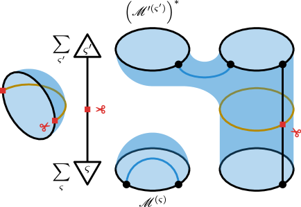
Figure 4: Slicing (orange and red) the gravitational path integral through cuts $C\in\mathcal{C}$ (red) of sources (black) gives states in sectors $\mathcal{H}_{C}$ of the gravitational Hilbert space.

In section 3.2, we defined the set $\mathcal{J}_{C}$ of partial sources associated with each cut $C\in\mathcal{C}$ to be a $\mathcal{J}$-module and thus a vector space over $\mathbb{C}$. We also required the path integral $\zeta:\mathcal{J}\to\mathbb{C}$ to be reflection-positive 56, such that it can be used in eq. 57 to define a $\mathbb{C}$-valued positive semi-definite Hermitian form $\innerproduct{\bullet}{\bullet}$ on $\mathcal{J}_{C}$. We can therefore build a Hilbert space $\mathcal{H}_{C}$ from $\mathcal{J}_{C}$ in the same manner as in section 2.3. First, we quotient $\mathcal{J}_{C}$ by the subspace

$$\mathcal{N}_{C} =\left\{J_{C}\in\mathcal{J}_{C}:\innerproduct{J_{C}^{\prime}}{J_{C}}=0\quad\forall J_{C}^{\prime}\in\mathcal{J}_{C}\right\}$$ (59)

of null vectors, obtaining a pre-Hilbert space $\mathcal{J}_{C}/\mathcal{N}_{C}$ with inner product $\innerproduct{\bullet}{\bullet}$. Then, we take the Hilbert space $\mathcal{H}_{C}$ to be the completion of $\mathcal{J}_{C}/\mathcal{N}_{C}$ with respect to the norm obtained from $\innerproduct{\bullet}{\bullet}$.

We would now like to construct $\alpha$-sectors $\mathcal{H}_{C}^{\alpha}$ of $\mathcal{H}_{C}$. One can do so like in section 2.3 by defining operators $Z(J)$ on $\mathcal{J}_{C}/\mathcal{N}_{C}$ as

$$Z(J)\ket{J_{C}} =\ket{J\sqcup J_{C}}\;.$$ (60)

Then, after making appropriate assumptions about extensions of bounded functions of operators to $\mathcal{H}_{C}$, one can again decompose $\mathcal{H}_{C}$ into $\alpha$-sectors $\mathcal{H}_{C}^{\alpha}$ where $Z(J)$ take definite eigenvalues $Z_{\alpha}(J)$. However, let us instead construct $\mathcal{H}_{C}^{\alpha}$ directly from the $\alpha$-sectors of the baby universe Hilbert space $\mathcal{H}_{\emptyset}^{\alpha}$, thus making it clear that the spectrum $\mathcal{A}$ of $Z(J)$ is the same on $\mathcal{H}_{C}$ as on the baby universe Hilbert space $\mathcal{H}_{\emptyset}$.

To do so, for all $C,C^{\prime}\in\mathcal{C}$ and $J_{C}\in\mathcal{J}_{C}$, let us start by defining an operator

$$\psi(J_{C}):\mathcal{J}_{C^{\prime}}/\mathcal{N}_{C^{\prime}} \to\mathcal{J}_{C\otimes C^{\prime}}/\mathcal{N}_{C\otimes C^{\prime}}\;, \ket{J_{C^{\prime}}} \mapsto\ket{J_{C}\otimes J_{C^{\prime}}}\;.$$ (61)

A side remark is that eq. 60 is a special case of eq. 61 with

$$Z(J)=\psi(J)$$ (62)

for $J\in\mathcal{J}=\mathcal{J}_{\emptyset}$. In the following, we will instead focus on the case $C^{\prime}=\emptyset$ while $C\in\mathcal{C}$ remains arbitrary in eq. 61. In this case, we extend $\psi(J_{C})$ to a domain including all $\alpha$-states in $\mathcal{H}_{\emptyset}$, such that the following continuity condition holds. Since $\alpha$-states $\ket{\alpha}$ span $\mathcal{H}_{\emptyset}$, we can decompose $\ket{J}$ for any $J\in\mathcal{J}$ as a sum or integral of $\ket{\alpha}$. The continuity condition we require is for $\psi(J_{C})$ to commute with performing this sum or integral — i.e., after acting on the summand or integrand with $\psi(J_{C})$, the sum or integral converges to $\psi(J_{C})\ket{J}=\ket{J\sqcup J_{C}}$ as expected from eq. 61.

We now define the Hilbert space $\mathcal{H}_{C}^{\alpha}$ to be the Cauchy completion of

$$\mathcal{D}_{C}^{\alpha} =\{\ket{J_{C},\alpha}_{\mathrm{r}}:J_{C}\in\mathcal{J}_{C}\}\;, \ket{J_{C},\alpha} =\psi(J_{C})\ket{\alpha}$$ (63)

(where the subscript on $\ket{J_{C},\alpha}_{\mathrm{r}}$ indicates a rescaling to be explained in the next paragraph). To see that $\mathcal{H}_{C}$ can be fully decomposed into such sectors, recall that the set of $\ket{J_{C}}=\psi(J_{C})\ket{\varnothing}$ for $J_{C}\in\mathcal{J}_{C}$ is a dense subspace. We can then apply our continuity condition to a decomposition of $\ket{\varnothing}$ in terms of $\ket{\alpha}$. It follows that summing over $\mathcal{D}_{C}^{\alpha}$ for all $\alpha$ and taking the Cauchy completion recovers the full Hilbert space

$$\mathcal{H}_{C} =\int_{\mathcal{A}}^{\oplus}\differential{\alpha}\mathcal{H}_{C}^{\alpha}\;.$$ (64)

As expressed above, the $\alpha$-sectors are mutually orthogonal. Indeed, as required by eq. 57 and our continuity condition,

$$\innerproduct{J_{C}^{\prime},\alpha^{\prime}}{J_{C},\alpha} =Z_{\alpha}(J_{C}^{\prime}|J_{C})\innerproduct{\alpha^{\prime}}{\alpha}\;,$$ (65)

for states in the dense subspaces $\mathcal{D}_{C}^{\alpha^{\prime}}$ and $\mathcal{D}_{C}^{\alpha}$; the inner products of more general states are limits of the above. Recall that $\innerproduct{\alpha^{\prime}}{\alpha}$ is equal to the $\delta$-function on $\mathcal{A}$. It will be convenient therefore to introduce the notation

$$\ket{\bullet,\alpha}_{\mathrm{r}} =\norm{\alpha}^{-1}\ket{\bullet,\alpha}$$ (66)

to denote states rescaled by the norm $\norm{\alpha}=\sqrt{\innerproduct{\alpha}{\alpha}}$ so that this possibly infinite factor does not appear in inner products within $\alpha$-sectors, e.g.

$$\tensor[_{\mathrm{r}}]{\innerproduct{J_{C}^{\prime},\alpha}{J_{C},\alpha}}{{}_{\mathrm{r}}} =Z_{\alpha}(J_{C}^{\prime}|J_{C})\;.$$ (67)

In section 2.3, baby universe $\alpha$-sectors $\mathcal{H}_{\emptyset}^{\alpha}$ were defined to be superselection sectors in which the operators $Z(J)$ take definite eigenvalues $Z_{\alpha}(J)$. It is clear from eqs. 60 and 61 that $Z(J)$ and $\psi(J_{C})$ commute on $\mathcal{J}/\mathcal{N}$. Therefore, it is natural to define an extension of $Z(J)$ which acts on each $\mathcal{H}_{C}^{\alpha}$ as multiplication by the constant $Z_{\alpha}(J)$. The consistency of this definition with eq. 60 follows from our continuity condition. Thus, the $\alpha$-sectors $\mathcal{H}_{C}^{\alpha}$ are again superselection sectors where the commuting operators $Z(J)$ take the definite eigenvalues $Z_{\alpha}(J)$.

An important point of departure from $\mathcal{H}_{\emptyset}^{\alpha}$, however, is that $\mathcal{H}_{C}^{\alpha}$ for $C\neq\emptyset$ is generically not one-dimensional. In particular, one can consider the closest analogue of eq. 24,

$$\innerproduct{\psi_{C},\alpha}{J\sqcup J_{C}} =\matrixelement{\psi_{C},\alpha}{Z(J)}{J_{C}}=Z_{\alpha}(J)\innerproduct{\psi_{C},\alpha}{J_{C}}\;,$$ (68)

for any $J\in\mathcal{J}$, $J_{C}\in\mathcal{J}_{C}$, and $\ket{\psi_{C},\alpha}_{\mathrm{r}}\in\mathcal{H}_{C}^{\alpha}$. For $C\neq\emptyset$, the $\mathcal{J}$-module $\mathcal{J}_{C}$ need not be cyclic, and eq. 68 can be consistent with the existence of many linearly independent states $\ket{\psi_{C},\alpha}_{\mathrm{r}}\in\mathcal{H}_{C}^{\alpha}$.

Let us end this section with two further remarks which will be of use in section 4.2. Firstly, we note that there is a natural isometric embedding $\mathcal{H}_{C}^{\alpha}\otimes\mathcal{H}_{C^{\prime}}^{\alpha}\to\mathcal{H}_{C\otimes{}C^{\prime}}^{\alpha}$. This is just the continuous extension of the isometric embedding

$$\mathcal{D}_{C}^{\alpha}\otimes\mathcal{D}_{C^{\prime}}^{\alpha} \to\mathcal{D}_{C\otimes C^{\prime}}^{\alpha}\;, \ket{J_{C},\alpha}_{\mathrm{r}}\otimes\ket{J_{C},\alpha}_{\mathrm{r}} \mapsto\ket{J_{C}\otimes J_{C^{\prime}},\alpha}_{\mathrm{r}}$$ (69)

More generally, we will write the embedding of arbitrary states similarly as

$$\mathcal{H}_{C}^{\alpha}\otimes\mathcal{H}_{C^{\prime}}^{\alpha} \to\mathcal{H}_{C\otimes C^{\prime}}^{\alpha}\;, \ket{\psi_{C},\alpha}_{\mathrm{r}}\otimes\ket{\psi_{C^{\prime}},\alpha}_{\mathrm{r}} \mapsto\ket{\psi_{C}\otimes\psi_{C^{\prime}},\alpha}_{\mathrm{r}}\;.$$ (70)

This embedding need not be onto, however. The Hilbert space $\mathcal{H}_{C\otimes{}C^{\prime}}^{\alpha}$ can thus fail to factorize into a tensor product of Hilbert spaces associated respectively with $C$ and $C^{\prime}$.

Secondly, we can construct an anti-isometry relating $\mathcal{H}_{C}^{\alpha}$ and $\mathcal{H}_{C^{*}}^{\alpha}$. Continuously extending

$$\mathcal{D}_{C}^{\alpha} \to\mathcal{D}_{C^{*}}^{\alpha}\;, \ket{J_{C},\alpha}_{\mathrm{r}} \mapsto\ket{J_{C}^{*},\alpha}_{\mathrm{r}}\;,$$ (71)

we will more generally write

$$\mathcal{H}_{C}^{\alpha} \to\mathcal{H}_{C^{*}}^{\alpha}\;, \ket{\psi_{C},\alpha}_{\mathrm{r}} \mapsto\ket{(\psi_{C})^{*},\alpha}_{\mathrm{r}}\;.$$ (72)

4 A noncommutative algebra of operators and bounds on $\alpha$-sectors

In section 2.3, we showed that $\alpha$-sectors $\mathcal{H}_{\emptyset}^{\alpha}$ in the baby universe Hilbert space $\mathcal{H}_{\emptyset}$ must be one-dimensional. The fact that each $\mathcal{H}_{\emptyset}^{\alpha}$ is one-dimensional is consistent with the lack of nontrivial operators on $\mathcal{H}_{\emptyset}^{\alpha}$. Recall that $\mathcal{H}_{\emptyset}$ is comprised of states of baby universes, which are closed universes on slices where sources for the gravitational path integral do not prescribe the existence of objects like spatial boundaries, observer worldlines, or nongravitational external systems. The lack of nontrivial operators can therefore be understood as a consequence of the lack of objects on these slices to which one can dress such operators.

In section 3.3, we explained that the $\alpha$-sectors $\mathcal{H}_{C}^{\alpha}$, in Hilbert spaces $\mathcal{H}_{C}$ of states prepared by partial sources with nontrivial cuts $C\neq\emptyset$, need not be one-dimensional. These states describe slices where sources for the gravitational path integral prescribe the existence of objects located at $C$, on which one can construct operators which remain generically nontrivial in each superselection $\mathcal{H}_{C}^{\alpha}$.

In section 4.1, we will construct some of these generically noncommuting operators on $\mathcal{H}_{C}^{\alpha}$ which act by gluing partial sources $J_{C\otimes{}C^{*}}\in\mathcal{J}_{C\otimes{}C^{*}}$ to states — this construction will parallel that of ref. Colafranceschi:2023moh . In section 4.2, we will then derive a bound on the Hilbert space trace of certain such operators in each $\mathcal{H}_{C}^{\alpha}$ using the Cauchy-Schwarz inequality. One can view the trace of positive operators as a proxy for measuring the size of $\mathcal{H}_{C}^{\alpha}$ and accordingly interpret our result as an upper bound on this size. This analysis will be a hybrid of similar analyses found in refs. Marolf:2020xie ; Colafranceschi:2023moh .

4.1 Non-superselected operators

Let us begin by defining some gluing operators on the dense domain $\mathcal{D}_{C}^{\alpha}$ of $\mathcal{H}_{C}^{\alpha}$. For each $J_{C\otimes{}C^{*}}\in\mathcal{J}_{C\otimes{}C^{*}}$, we define the operator $O(J_{C\otimes{}C^{*}})$ on this domain using the gluing operation introduced in eq. 50,

$$O(J_{C\otimes{}C^{*}}):\mathcal{D}_{C}^{\alpha} \to\mathcal{D}_{C}^{\alpha}\;, \ket{J_{C},\alpha}_{\mathrm{r}}\mapsto\Big{|}J_{C\otimes\mathchoice{\leavevmode\hbox to6.23pt{\vbox to4.78pt{\text{[drawing]}}}}{\leavevmode\hbox to6.23pt{\vbox to4.78pt{\text{[drawing]}}}}{\leavevmode\hbox to3.85pt{\vbox to3.35pt{\text{[drawing]}}}}{\leavevmode\hbox to2.75pt{\vbox to2.39pt{\text{[drawing]}}}}^{*}}\otimes J_{\mathchoice{\leavevmode\hbox to6.23pt{\vbox to4.78pt{\text{[drawing]}}}}{\leavevmode\hbox to6.23pt{\vbox to4.78pt{\text{[drawing]}}}}{\leavevmode\hbox to3.85pt{\vbox to3.35pt{\text{[drawing]}}}}{\leavevmode\hbox to2.75pt{\vbox to2.39pt{\text{[drawing]}}}}},\alpha\Big{\rangle}_{\mathrm{r}}\;.\leavevmode\hbox to0pt{\vbox to0pt{\text{[drawing]}}} \scriptstyle C \scriptstyle C$$ (73)

Before extending $O(J_{C\otimes{}C^{*}})$ to $\mathcal{H}_{C}^{\alpha}$, let us make some preliminary observations about these operators defined on $\mathcal{D}_{C}^{\alpha}$.

The first is that the product of two such operators 73 is another,

$$O(J_{C\otimes{}C^{*}})O(J_{C\otimes{}C^{*}}^{\prime}) =O\Big{(}J_{C\otimes{}\mathchoice{\leavevmode\hbox to6.23pt{\vbox to4.78pt{\text{[drawing]}}}}{\leavevmode\hbox to6.23pt{\vbox to4.78pt{\text{[drawing]}}}}{\leavevmode\hbox to3.85pt{\vbox to3.35pt{\text{[drawing]}}}}{\leavevmode\hbox to2.75pt{\vbox to2.39pt{\text{[drawing]}}}}^{*}}\otimes J_{\mathchoice{\leavevmode\hbox to6.23pt{\vbox to4.78pt{\text{[drawing]}}}}{\leavevmode\hbox to6.23pt{\vbox to4.78pt{\text{[drawing]}}}}{\leavevmode\hbox to3.85pt{\vbox to3.35pt{\text{[drawing]}}}}{\leavevmode\hbox to2.75pt{\vbox to2.39pt{\text{[drawing]}}}}\otimes{}C^{*}}^{\prime}\Big{)}\;.\leavevmode\hbox to0pt{\vbox to0pt{\text{[drawing]}}} \scriptstyle C \scriptstyle C$$ (74)

We see from this expression that, with the exception of $C=\emptyset$ (in which case $O(J)=Z(J)$ for $J\in\mathcal{J}$), the operators $O$ are not generically expected to commute,

$$O(J_{C\otimes{}C^{*}})\,O(J_{C\otimes{}C^{*}}^{\prime}) \neq O(J_{C\otimes{}C^{*}}^{\prime})\,O(J_{C\otimes{}C^{*}})\;,$$ (75)

for distinct $J_{C\otimes{}C^{*}},J_{C\otimes{}C^{*}}^{\prime}\in\mathcal{J}_{C\otimes{}C^{*}}$. If this is the case on $\mathcal{D}_{C}^{\alpha}$, then any extensions of the operators will also fail to commute.

Secondly, for states in $\mathcal{D}_{C}^{\alpha}$, it is straightforward to show from eqs. 57 and 53 that matrix elements of the adjoint $O(J_{C\otimes{}C^{*}})^{\dagger}$ are equal to

$$\tensor[_{\mathrm{r}}]{\matrixelement{J^{\prime}_{C},\alpha}{O(J_{C\otimes{}C^{*}})^{\dagger}}{J_{C},\alpha}}{{}_{\mathrm{r}}} =\tensor[_{\mathrm{r}}]{\matrixelement{J^{\prime}_{C},\alpha}{O\Big{(}(J_{\mathchoice{\leavevmode\hbox to6.23pt{\vbox to4.78pt{\text{[drawing]}}}}{\leavevmode\hbox to6.23pt{\vbox to4.78pt{\text{[drawing]}}}}{\leavevmode\hbox to3.85pt{\vbox to3.35pt{\text{[drawing]}}}}{\leavevmode\hbox to2.75pt{\vbox to2.39pt{\text{[drawing]}}}}\otimes{}\mathchoice{\leavevmode\hbox to6.23pt{\vbox to4.78pt{\text{[drawing]}}}}{\leavevmode\hbox to6.23pt{\vbox to4.78pt{\text{[drawing]}}}}{\leavevmode\hbox to3.85pt{\vbox to3.35pt{\text{[drawing]}}}}{\leavevmode\hbox to2.75pt{\vbox to2.39pt{\text{[drawing]}}}}^{*}})^{*}\Big{)}}{J_{C},\alpha}}{{}_{\mathrm{r}}}\;.\leavevmode\hbox to0pt{\vbox to0pt{\text{[drawing]}}} \scriptstyle C \scriptstyle C$$ (76)

Therefore, if the reality condition

$$J_{C\otimes{}C^{*}} =(J_{\mathchoice{\leavevmode\hbox to6.23pt{\vbox to4.78pt{\text{[drawing]}}}}{\leavevmode\hbox to6.23pt{\vbox to4.78pt{\text{[drawing]}}}}{\leavevmode\hbox to3.85pt{\vbox to3.35pt{\text{[drawing]}}}}{\leavevmode\hbox to2.75pt{\vbox to2.39pt{\text{[drawing]}}}}\otimes{}\mathchoice{\leavevmode\hbox to6.23pt{\vbox to4.78pt{\text{[drawing]}}}}{\leavevmode\hbox to6.23pt{\vbox to4.78pt{\text{[drawing]}}}}{\leavevmode\hbox to3.85pt{\vbox to3.35pt{\text{[drawing]}}}}{\leavevmode\hbox to2.75pt{\vbox to2.39pt{\text{[drawing]}}}}^{*}})^{*}\leavevmode\hbox to0pt{\vbox to0pt{\text{[drawing]}}} \scriptstyle C \scriptstyle C$$ (77)

is satisfied, then the matrix elements of $O(J_{C\otimes{}C^{*}})$ in $\mathcal{D}_{C}^{\alpha}$ form a Hermitian matrix. Moreover, if $J_{C\otimes{}C^{*}}$ takes the form

$$J_{C\otimes{}C^{*}} =J_{C\otimes\mathchoice{\leavevmode\hbox to6.23pt{\vbox to4.78pt{\text{[drawing]}}}}{\leavevmode\hbox to6.23pt{\vbox to4.78pt{\text{[drawing]}}}}{\leavevmode\hbox to3.85pt{\vbox to3.35pt{\text{[drawing]}}}}{\leavevmode\hbox to2.75pt{\vbox to2.39pt{\text{[drawing]}}}}^{\prime}}\otimes(J_{C\otimes\mathchoice{\leavevmode\hbox to6.23pt{\vbox to4.78pt{\text{[drawing]}}}}{\leavevmode\hbox to6.23pt{\vbox to4.78pt{\text{[drawing]}}}}{\leavevmode\hbox to3.85pt{\vbox to3.35pt{\text{[drawing]}}}}{\leavevmode\hbox to2.75pt{\vbox to2.39pt{\text{[drawing]}}}}^{\prime}})^{*}\leavevmode\hbox to0pt{\vbox to0pt{\text{[drawing]}}} \scriptstyle C \scriptstyle C$$ (78)

for some $J_{C\otimes{}C^{\prime}}\in\mathcal{J}_{C\otimes{}C^{\prime}}$, then it is straightforward to show, using the positive definiteness 57 of the inner product, that expectation values of $O(J_{C\otimes{}C^{*}})$ in $\mathcal{D}_{C}^{\alpha}$ are non-negative,

$$\tensor[_{\mathrm{r}}]{\langle J_{C},\alpha|O\Big{(}J_{C\otimes\mathchoice{\leavevmode\hbox to6.23pt{\vbox to4.78pt{\text{[drawing]}}}}{\leavevmode\hbox to6.23pt{\vbox to4.78pt{\text{[drawing]}}}}{\leavevmode\hbox to3.85pt{\vbox to3.35pt{\text{[drawing]}}}}{\leavevmode\hbox to2.75pt{\vbox to2.39pt{\text{[drawing]}}}}^{\prime}}\otimes(J_{C\otimes\mathchoice{\leavevmode\hbox to6.23pt{\vbox to4.78pt{\text{[drawing]}}}}{\leavevmode\hbox to6.23pt{\vbox to4.78pt{\text{[drawing]}}}}{\leavevmode\hbox to3.85pt{\vbox to3.35pt{\text{[drawing]}}}}{\leavevmode\hbox to2.75pt{\vbox to2.39pt{\text{[drawing]}}}}^{\prime}})^{*}\Big{)}|J_{C},\alpha\rangle}{{}_{\mathrm{r}}} \scriptstyle C \scriptstyle C \geq 0\;.\leavevmode\hbox to0pt{\vbox to0pt{\text{[drawing]}}}$$ (79)

We would now like to continuously extend $O(J_{C\otimes{}C^{*}})$, for any $J_{C\otimes{}C^{*}}\in\mathcal{J}_{C\otimes{}C^{*}}$, to all of $\mathcal{H}_{C}^{\alpha}$, where we will argue by continuity that the above statements continue to hold. To see that this is possible, we will bound the operator norm of $O(J_{C\otimes{}C^{*}})$. Consider therefore the squared norm of an image state, which we can write using eq. 67 as

$$\tensor[_{\mathrm{r}}]{\Big{\langle}J_{C\otimes\mathchoice{\leavevmode\hbox to6.23pt{\vbox to4.78pt{\text{[drawing]}}}}{\leavevmode\hbox to6.23pt{\vbox to4.78pt{\text{[drawing]}}}}{\leavevmode\hbox to3.85pt{\vbox to3.35pt{\text{[drawing]}}}}{\leavevmode\hbox to2.75pt{\vbox to2.39pt{\text{[drawing]}}}}^{*}}\otimes J_{\mathchoice{\leavevmode\hbox to6.23pt{\vbox to4.78pt{\text{[drawing]}}}}{\leavevmode\hbox to6.23pt{\vbox to4.78pt{\text{[drawing]}}}}{\leavevmode\hbox to3.85pt{\vbox to3.35pt{\text{[drawing]}}}}{\leavevmode\hbox to2.75pt{\vbox to2.39pt{\text{[drawing]}}}}},\alpha\Big{|}J_{C\otimes\mathchoice{\leavevmode\hbox to6.23pt{\vbox to4.78pt{\text{[drawing]}}}}{\leavevmode\hbox to6.23pt{\vbox to4.78pt{\text{[drawing]}}}}{\leavevmode\hbox to3.85pt{\vbox to3.35pt{\text{[drawing]}}}}{\leavevmode\hbox to2.75pt{\vbox to2.39pt{\text{[drawing]}}}}^{*}}\otimes J_{\mathchoice{\leavevmode\hbox to6.23pt{\vbox to4.78pt{\text{[drawing]}}}}{\leavevmode\hbox to6.23pt{\vbox to4.78pt{\text{[drawing]}}}}{\leavevmode\hbox to3.85pt{\vbox to3.35pt{\text{[drawing]}}}}{\leavevmode\hbox to2.75pt{\vbox to2.39pt{\text{[drawing]}}}}},\alpha\Big{\rangle}}{{}_{\mathrm{r}}} \scriptstyle C \scriptstyle C \scriptstyle C \scriptstyle C =Z_{\alpha}\Big{(}(J_{\mathchoice{\leavevmode\hbox to6.23pt{\vbox to4.78pt{\text{[drawing]}}}}{\leavevmode\hbox to6.23pt{\vbox to4.78pt{\text{[drawing]}}}}{\leavevmode\hbox to3.85pt{\vbox to3.35pt{\text{[drawing]}}}}{\leavevmode\hbox to2.75pt{\vbox to2.39pt{\text{[drawing]}}}}\otimes\mathchoice{\leavevmode\hbox to6.23pt{\vbox to4.78pt{\text{[drawing]}}}}{\leavevmode\hbox to6.23pt{\vbox to4.78pt{\text{[drawing]}}}}{\leavevmode\hbox to3.85pt{\vbox to3.35pt{\text{[drawing]}}}}{\leavevmode\hbox to2.75pt{\vbox to2.39pt{\text{[drawing]}}}}^{*}})^{*}\otimes(J_{\mathchoice{\leavevmode\hbox to6.23pt{\vbox to4.78pt{\text{[drawing]}}}}{\leavevmode\hbox to6.23pt{\vbox to4.78pt{\text{[drawing]}}}}{\leavevmode\hbox to3.85pt{\vbox to3.35pt{\text{[drawing]}}}}{\leavevmode\hbox to2.75pt{\vbox to2.39pt{\text{[drawing]}}}}})^{*}\otimes J_{\mathchoice{\leavevmode\hbox to6.23pt{\vbox to4.78pt{\text{[drawing]}}}}{\leavevmode\hbox to6.23pt{\vbox to4.78pt{\text{[drawing]}}}}{\leavevmode\hbox to3.85pt{\vbox to3.35pt{\text{[drawing]}}}}{\leavevmode\hbox to2.75pt{\vbox to2.39pt{\text{[drawing]}}}}\otimes\mathchoice{\leavevmode\hbox to6.23pt{\vbox to4.78pt{\text{[drawing]}}}}{\leavevmode\hbox to6.23pt{\vbox to4.78pt{\text{[drawing]}}}}{\leavevmode\hbox to3.85pt{\vbox to3.35pt{\text{[drawing]}}}}{\leavevmode\hbox to2.75pt{\vbox to2.39pt{\text{[drawing]}}}}^{*}}\otimes J_{\mathchoice{\leavevmode\hbox to6.23pt{\vbox to4.78pt{\text{[drawing]}}}}{\leavevmode\hbox to6.23pt{\vbox to4.78pt{\text{[drawing]}}}}{\leavevmode\hbox to3.85pt{\vbox to3.35pt{\text{[drawing]}}}}{\leavevmode\hbox to2.75pt{\vbox to2.39pt{\text{[drawing]}}}}}\Big{)} \scriptstyle C \scriptstyle C \scriptstyle C \scriptstyle C \scriptstyle C \scriptstyle C$$ (80)

$$=\tensor[_{\mathrm{r}}]{\Big{\langle}J_{C\otimes\mathchoice{\leavevmode\hbox to6.23pt{\vbox to4.78pt{\text{[drawing]}}}}{\leavevmode\hbox to6.23pt{\vbox to4.78pt{\text{[drawing]}}}}{\leavevmode\hbox to3.85pt{\vbox to3.35pt{\text{[drawing]}}}}{\leavevmode\hbox to2.75pt{\vbox to2.39pt{\text{[drawing]}}}}^{*}}\otimes(J_{\mathchoice{\leavevmode\hbox to6.23pt{\vbox to4.78pt{\text{[drawing]}}}}{\leavevmode\hbox to6.23pt{\vbox to4.78pt{\text{[drawing]}}}}{\leavevmode\hbox to3.85pt{\vbox to3.35pt{\text{[drawing]}}}}{\leavevmode\hbox to2.75pt{\vbox to2.39pt{\text{[drawing]}}}}})^{*},\alpha\Big{|}J_{C\otimes C^{*}}\otimes(J_{C})^{*},\alpha\Big{\rangle}}{{}_{\mathrm{r}}}\;.\leavevmode\hbox to0pt{\vbox to0pt{\text{[drawing]}}} \scriptstyle C \scriptstyle C$$ (81)

We can now apply the Cauchy-Schwarz inequality,

$$\absolutevalue{\innerproduct{\psi^{\prime}}{\psi}}\leq\norm{\psi^{\prime}}\,\norm{\psi\vphantom{{}^{\prime}}}\;,$$ (82)

which follows simply from the positive definiteness of the inner product,

$$0 \leq\min_{z\in\mathbb{C}}\norm{z\,\psi+\psi^{\prime}}=\norm{-\frac{\absolutevalue{\innerproduct{\psi^{\prime}}{\psi}}^{2}}{\norm{\psi}^{2}\innerproduct{\psi^{\prime}}{\psi}}\,\psi+\psi^{\prime}}=-\frac{\absolutevalue{\innerproduct{\psi^{\prime}}{\psi}}^{2}}{\norm{\psi}^{2}}+\norm{\psi^{\prime}}^{2}\;.$$ (83)

Upon applying the Cauchy-Schwarz inequality to the RHS of eq. 81, a short calculation shows that the operator norm $\norm{O(J_{C\otimes{}C^{*}})}$ is bounded by

$$\norm{O(J_{C\otimes{}C^{*}})}\leq\sqrt{\tensor[_{\mathrm{r}}]{\innerproduct{J_{C\otimes C^{*}},\alpha}{J_{C\otimes C^{*}},\alpha}}{{}_{\mathrm{r}}}}=\sqrt{Z_{\alpha}(J_{C\otimes C^{*}}|J_{C\otimes C^{*}})}\;.$$ (84)

For fixed $\alpha$, we expect $Z_{\alpha}(J_{C\otimes C^{*}}|J_{C\otimes C^{*}})$ to be finite. If this is case, we can continuously extend the densely-defined bounded operator $O(J_{C\otimes{}C^{*}})$ to all of $\mathcal{H}_{C}^{\alpha}$.

By continuity, eq. 74 applies to these extended operators on $\mathcal{H}_{C}^{\alpha}$. Continuity of eq. 76 implies that the adjoint is indeed given by

$$O(J_{C\otimes{}C^{*}})^{\dagger} =O\Big{(}(J_{\mathchoice{\leavevmode\hbox to6.23pt{\vbox to4.78pt{\text{[drawing]}}}}{\leavevmode\hbox to6.23pt{\vbox to4.78pt{\text{[drawing]}}}}{\leavevmode\hbox to3.85pt{\vbox to3.35pt{\text{[drawing]}}}}{\leavevmode\hbox to2.75pt{\vbox to2.39pt{\text{[drawing]}}}}\otimes{}\mathchoice{\leavevmode\hbox to6.23pt{\vbox to4.78pt{\text{[drawing]}}}}{\leavevmode\hbox to6.23pt{\vbox to4.78pt{\text{[drawing]}}}}{\leavevmode\hbox to3.85pt{\vbox to3.35pt{\text{[drawing]}}}}{\leavevmode\hbox to2.75pt{\vbox to2.39pt{\text{[drawing]}}}}^{*}})^{*}\Big{)}\;.\leavevmode\hbox to0pt{\vbox to0pt{\text{[drawing]}}} \scriptstyle C \scriptstyle C$$ (85)

In particular, partial sources that satisfy eq. 77 give rise to self-adjoint $O(J_{C\otimes{}C^{*}})$, while continuity of eq. 79 shows that those of the form 78 give positive semi-definite $O(J_{C\otimes{}C^{*}})$.

4.2 Bounds on $\alpha$-sectors $\mathcal{H}_{C}^{\alpha}$

The dimension of a finite-dimensional Hilbert space is simply given by the Hilbert space trace of the identity operator. To get a finite notion of size in an infinite-dimensional Hilbert space, however, it is often useful to look at the trace of operators such as $e^{-\beta H}$, where $H$ is the Hamiltonian of the system. We will return to this example in section 5.1.

In the remainder of this section, we will more generally consider operators $O(J_{C\otimes{}C^{*}})$ of the kind introduced in section 4.1, in the case where $J_{C\otimes{}C^{*}}$ takes the form

$$J_{C\otimes{}C^{*}} =J_{C\otimes\mathchoice{\leavevmode\hbox to6.23pt{\vbox to4.78pt{\text{[drawing]}}}}{\leavevmode\hbox to6.23pt{\vbox to4.78pt{\text{[drawing]}}}}{\leavevmode\hbox to3.85pt{\vbox to3.35pt{\text{[drawing]}}}}{\leavevmode\hbox to2.75pt{\vbox to2.39pt{\text{[drawing]}}}}^{*}}^{\nicefrac{{1}}{{2}}}\otimes J_{\mathchoice{\leavevmode\hbox to6.23pt{\vbox to4.78pt{\text{[drawing]}}}}{\leavevmode\hbox to6.23pt{\vbox to4.78pt{\text{[drawing]}}}}{\leavevmode\hbox to3.85pt{\vbox to3.35pt{\text{[drawing]}}}}{\leavevmode\hbox to2.75pt{\vbox to2.39pt{\text{[drawing]}}}}\otimes{}C^{*}}^{\nicefrac{{1}}{{2}}}\leavevmode\hbox to0pt{\vbox to0pt{\text{[drawing]}}} \scriptstyle C \scriptstyle C$$ (86)

for some

$$J_{C\otimes{}C^{*}}^{1/2} =\Big{(}J_{\mathchoice{\leavevmode\hbox to6.23pt{\vbox to4.78pt{\text{[drawing]}}}}{\leavevmode\hbox to6.23pt{\vbox to4.78pt{\text{[drawing]}}}}{\leavevmode\hbox to3.85pt{\vbox to3.35pt{\text{[drawing]}}}}{\leavevmode\hbox to2.75pt{\vbox to2.39pt{\text{[drawing]}}}}\otimes{}\mathchoice{\leavevmode\hbox to6.23pt{\vbox to4.78pt{\text{[drawing]}}}}{\leavevmode\hbox to6.23pt{\vbox to4.78pt{\text{[drawing]}}}}{\leavevmode\hbox to3.85pt{\vbox to3.35pt{\text{[drawing]}}}}{\leavevmode\hbox to2.75pt{\vbox to2.39pt{\text{[drawing]}}}}^{*}}^{1/2}\Big{)}^{*}\in\mathcal{J}_{C\otimes{}C^{*}}\;.\leavevmode\hbox to0pt{\vbox to0pt{\text{[drawing]}}} \scriptstyle C \scriptstyle C$$ (87)

Then, $O\left(J_{C\otimes{}C^{*}}^{1/2}\right)$ is self-adjoint and

$$O(J_{C\otimes{}C^{*}}) =O\left(J_{C\otimes{}C^{*}}^{1/2}\right)^{2}$$ (88)

is positive semi-definite. We will now show that the Hilbert space trace of $O(J_{C\otimes{}C^{*}})$ on $\mathcal{H}_{C}^{\alpha}$ is bounded by a path integral,

$$\sum_{\gamma}\lambda_{\gamma}^{\alpha} \leq Z_{\alpha}\Big{(}J_{\mathchoice{\leavevmode\hbox to6.23pt{\vbox to4.78pt{\text{[drawing]}}}}{\leavevmode\hbox to6.23pt{\vbox to4.78pt{\text{[drawing]}}}}{\leavevmode\hbox to3.85pt{\vbox to3.35pt{\text{[drawing]}}}}{\leavevmode\hbox to2.75pt{\vbox to2.39pt{\text{[drawing]}}}}\otimes\mathchoice{\leavevmode\hbox to6.23pt{\vbox to4.78pt{\text{[drawing]}}}}{\leavevmode\hbox to6.23pt{\vbox to4.78pt{\text{[drawing]}}}}{\leavevmode\hbox to3.85pt{\vbox to3.35pt{\text{[drawing]}}}}{\leavevmode\hbox to2.75pt{\vbox to2.39pt{\text{[drawing]}}}}^{*}}\Big{)}\;,\leavevmode\hbox to0pt{\vbox to0pt{\text{[drawing]}}} \scriptstyle C \scriptstyle C$$ (89)

where $\lambda_{\gamma}^{\alpha}$ are eigenvalues of $O(J_{C\otimes{}C^{*}})$ on $\mathcal{H}_{C}^{\alpha}$ and degeneracies are included in the sum.

Let $\ket{\psi_{C}^{\gamma},\alpha}_{\mathrm{r}}\in\mathcal{H}_{C}^{\alpha}$ be an orthonormal basis of eigenstates for which

$$O\left(J_{C\otimes{}C^{*}}^{1/2}\right)\ket{\psi_{C}^{\gamma},\alpha}_{\mathrm{r}} =\left(\lambda_{\gamma}^{\alpha}\right)^{1/2}\ket{\psi_{C}^{\gamma},\alpha}_{\mathrm{r}}\;, O\left(J_{C\otimes{}C^{*}}\right)\ket{\psi_{C}^{\gamma},\alpha}_{\mathrm{r}} =\lambda_{\gamma}^{\alpha}\ket{\psi_{C}^{\gamma},\alpha}_{\mathrm{r}}\;.$$ (90)

We would like to apply the Cauchy-Schwarz inequality 82 to the states $\ket{J_{C\otimes{}C^{*}}^{1/2},\alpha}_{\mathrm{r}}$ and

$$\ket{\mathrm{TFD}_{C\otimes C^{*}},\alpha}_{\mathrm{r}} =\sum_{\gamma}\left(\lambda_{\gamma}^{\alpha}\right)^{1/2}\,\ket{\psi_{C}^{\gamma}\otimes(\psi_{C}^{\gamma})^{*},\alpha}_{\mathrm{r}}\;.$$ (91)

To that end, we evaluate the inner products

$$\tensor[_{\mathrm{r}}]{\innerproduct{J_{C\otimes{}C^{*}}^{1/2},\alpha}{J_{C\otimes{}C^{*}}^{1/2},\alpha}}{{}_{\mathrm{r}}} =Z_{\alpha}\left(J_{C\otimes{}C^{*}}^{1/2}\middle|J_{C\otimes{}C^{*}}^{1/2}\right)=Z_{\alpha}\Big{(}J_{\mathchoice{\leavevmode\hbox to6.23pt{\vbox to4.78pt{\text{[drawing]}}}}{\leavevmode\hbox to6.23pt{\vbox to4.78pt{\text{[drawing]}}}}{\leavevmode\hbox to3.85pt{\vbox to3.35pt{\text{[drawing]}}}}{\leavevmode\hbox to2.75pt{\vbox to2.39pt{\text{[drawing]}}}}\otimes\mathchoice{\leavevmode\hbox to6.23pt{\vbox to4.78pt{\text{[drawing]}}}}{\leavevmode\hbox to6.23pt{\vbox to4.78pt{\text{[drawing]}}}}{\leavevmode\hbox to3.85pt{\vbox to3.35pt{\text{[drawing]}}}}{\leavevmode\hbox to2.75pt{\vbox to2.39pt{\text{[drawing]}}}}^{*}}\Big{)}\;, \scriptstyle C \scriptstyle C$$ (92)

$$\tensor[_{\mathrm{r}}]{\innerproduct{\mathrm{TFD}_{C\otimes C^{*}},\alpha}{J_{C\otimes{}C^{*}}^{1/2},\alpha}}{{}_{\mathrm{r}}} =\sum_{\gamma}\left(\lambda_{\gamma}^{\alpha}\right)^{1/2}\,\tensor[_{\mathrm{r}}]{\innerproduct{\psi_{C}^{\gamma}\otimes(\psi_{C}^{\gamma})^{*},\alpha}{J_{C\otimes{}C^{*}}^{1/2},\alpha}}{{}_{\mathrm{r}}}$$ (93)

$$=\sum_{\gamma}\left(\lambda_{\gamma}^{\alpha}\right)^{1/2}\,\tensor[_{\mathrm{r}}]{\matrixelement{\psi_{C}^{\gamma},\alpha}{O\left(J_{C\otimes{}C^{*}}^{1/2}\right)}{\psi_{C}^{\gamma},\alpha}}{{}_{\mathrm{r}}}$$ (94)

$$=\sum_{\gamma}\lambda_{\gamma}^{\alpha}$$ (95)

$$=\tensor[_{\mathrm{r}}]{\innerproduct{\mathrm{TFD}_{C\otimes C^{*}},\alpha}{\mathrm{TFD}_{C\otimes C^{*}},\alpha}}{{}_{\mathrm{r}}}\;,\leavevmode\hbox to0pt{\vbox to0pt{\text{[drawing]}}}$$ (96)

where eq. 94 follows from the continuity of $O\left(J_{C\otimes{}C^{*}}^{1/2}\right)$ and replacing $\ket{\psi_{C}^{\gamma},\alpha}_{\mathrm{r}}$ by limits of $\ket{J_{C},\alpha}_{\mathrm{r}}\in\mathcal{D}_{C}^{\alpha}$, which we can more easily manipulate using eqs. 53, 67 and 73. The Cauchy-Schwarz inequality 82 then gives the desired bound 89 on the Hilbert space trace of $O(J_{C\otimes{}C^{*}})$ on $\mathcal{H}_{C}^{\alpha}$.

The constructive derivation 83 of the Cauchy-Schwarz inequality also tells us that 89 is saturated if and only if

$$\ket{J_{C\otimes{}C^{*}}^{1/2},\alpha}_{\mathrm{r}}=\ket{\mathrm{TFD}_{C\otimes C^{*}},\alpha}_{\mathrm{r}}\;.$$ (97)

Recall, as described below eq. 70, that the Hilbert space $\mathcal{H}_{C\otimes{}C^{*}}^{\alpha}$ need not factorize Harlow:2015lma ; Colafranceschi:2023moh between the cut components $C$ and $C^{*}$, and $\mathcal{H}_{C}^{\alpha}\otimes\mathcal{H}_{C^{*}}^{\alpha}\ni\ket{\mathrm{TFD}_{C\otimes{}C^{*}},\alpha}_{\mathrm{r}}$ might be a proper subspace of $\mathcal{H}_{C\otimes{}C^{*}}^{\alpha}\ni\ket{J_{C\otimes{}C^{*}}^{1/2},\alpha}_{\mathrm{r}}$. Therefore, eq. 97 need not hold and the bound 89 need not be saturated.

Let us remark finally that while path integrals $\zeta_{\alpha}=Z_{\alpha}$ restricted to $\alpha$-sectors are practically inaccessible (except in simple toy theories), we can take the ensemble average of eq. 89 to obtain a useful bound involving the original, generically non-factorizing path integral $\zeta$:

$$\int_{\mathcal{A}}\differential{\alpha}\absolutevalue{\innerproduct{\alpha}{\varnothing}}^{2}\,\sum_{\gamma}\lambda_{\gamma}^{\alpha} \leq\zeta\Big{(}J_{\mathchoice{\leavevmode\hbox to6.23pt{\vbox to4.78pt{\text{[drawing]}}}}{\leavevmode\hbox to6.23pt{\vbox to4.78pt{\text{[drawing]}}}}{\leavevmode\hbox to3.85pt{\vbox to3.35pt{\text{[drawing]}}}}{\leavevmode\hbox to2.75pt{\vbox to2.39pt{\text{[drawing]}}}}\otimes\mathchoice{\leavevmode\hbox to6.23pt{\vbox to4.78pt{\text{[drawing]}}}}{\leavevmode\hbox to6.23pt{\vbox to4.78pt{\text{[drawing]}}}}{\leavevmode\hbox to3.85pt{\vbox to3.35pt{\text{[drawing]}}}}{\leavevmode\hbox to2.75pt{\vbox to2.39pt{\text{[drawing]}}}}^{*}}\Big{)}\;.\leavevmode\hbox to0pt{\vbox to0pt{\text{[drawing]}}} \scriptstyle C \scriptstyle C$$ (98)

This provides an upper bound on the $\alpha$-dependent trace $\sum_{\gamma}\lambda_{\gamma}^{\alpha}$ averaged over the Hartle-Hawking ensemble.

5 Discussion

In this paper, we have developed a framework which describes the gravitational path integral and corresponding Hilbert spaces in terms of abstract sources and partial sources.

In particular, we described in section 2.2 the gravitational path integral as a function from the commutative $*$-algebra of sources $\mathcal{J}$ to $\mathbb{C}$. In section 2.3, we then constructed the Hilbert space $\mathcal{H}_{\emptyset}$ of baby universe states prepared by the insertion of sources $J\in\mathcal{J}$ in the path integral. We saw in particular that $\mathcal{H}_{\emptyset}$ decomposes into superselection sectors $\mathcal{H}_{\emptyset}^{\alpha}$ which are one-dimensional. Viewing each $\alpha$-sector $\mathcal{H}_{\emptyset}^{\alpha}$ as describing a self-contained UV-complete theory of gravity, this leads to the striking conclusion that there is a unique state of freely fluctuating closed universes in each such theory.

In section 3.2, we generalized our framework to include $\mathcal{J}$-modules $\mathcal{J}_{C}$ of partial sources $J_{C}\in\mathcal{J}_{C}$ which, when appropriately glued across the cut $C\in\mathcal{C}$, produce complete sources $J\in\mathcal{J}$. We then used these partial sources in section 3.3 to prepare states in Hilbert space sectors $\mathcal{H}_{C}$ labelled by cuts $C$. Importantly, $\mathcal{H}_{C}$ decomposes into $\alpha$-sectors $\mathcal{H}_{C}^{\alpha}$ which can have dimension greater than one. In particular, we constructed in section 4.1 a noncommutative algebra of operators $O(J_{C\otimes{}C^{*}}):\mathcal{H}_{C}^{\alpha}\to\mathcal{H}_{C}^{\alpha}$.

In section 5.1, we will first review how spacetimes with spatial boundaries fit into our framework of partial sources and cuts Marolf:2020xie . Then in section 5.2, we will demonstrate how our abstract formalism also encapsulates recent proposals for modifying rules of the gravitational path integral, such that closed universes no longer have one-dimensional Hilbert spaces when observers are included Abdalla:2025gzn ; Harlow:2025pvj . We will moreover apply the bound we derived in section 4.2 on the Hilbert space trace of $O(J_{C\otimes{}C^{*}})$ in $\mathcal{H}_{C}^{\alpha}$, finding rough agreement with bounds on the dimension of $\mathcal{H}_{C}^{\alpha}$ reported by refs. Abdalla:2025gzn ; Harlow:2025pvj in simple theories. We end in section 5.3 by pointing to directions for future work.

5.1 Application to spatial boundaries

As described in section 2.1, some examples of sources $J\in\mathcal{J}$ are boundary manifolds $J=\mathscr{M}$ on which boundary conditions are prescribed for a bulk path integral. As described in section 3.1, examples of partial sources $J_{C}\in\mathcal{J}_{C}$ are partial boundary manifolds $J_{C}=\mathscr{N}_{\Sigma}$. The cut $C=\Sigma$ in this case is the boundary $\Sigma=\partial\mathscr{N}_{\Sigma}$ of the partial boundary manifold. From the bulk perspective, $\Sigma$ is also the boundary of a bulk codimension-one slice; taking this bulk slice to be a Cauchy slice of a Lorentzian section, $\Sigma$ is then a spatial boundary of this Cauchy slice. As described in section 3.3, we can construct the Hilbert space $\mathcal{H}_{\Sigma}$ of bulk spacetimes with spatial boundary $\Sigma$. In particular, its $\alpha$-sectors $\mathcal{H}_{\Sigma}^{\alpha}$ need not be one-dimensional, as was the case for baby universe, i.e. freely fluctuating closed universes.

Let us now consider in this context an example of the kind of operator $O(J_{C\otimes C^{*}})$ described in section 4. In particular, let $J_{C\otimes{}C^{*}}=\mathrm{Cyl}_{\Sigma\otimes{}\Sigma^{*}}^{\beta}$ be a partial boundary manifold which is a Euclidean cylinder, $\Sigma\times(0,\beta)$, prescribing boundary conditions which are invariant under translation along the Euclidean time interval $(0,\beta)$. Then this cylinder can be decomposed into two halves, as in 86,

$$\mathrm{Cyl}_{\Sigma\otimes{}\Sigma^{*}}^{\beta} =\mathrm{Cyl}_{\Sigma\otimes\mathchoice{\leavevmode\hbox to5.71pt{\vbox to4.78pt{\text{[drawing]}}}}{\leavevmode\hbox to5.71pt{\vbox to4.78pt{\text{[drawing]}}}}{\leavevmode\hbox to3.54pt{\vbox to3.35pt{\text{[drawing]}}}}{\leavevmode\hbox to2.53pt{\vbox to2.39pt{\text{[drawing]}}}}^{*}}^{\beta/2}\otimes\mathrm{Cyl}_{\mathchoice{\leavevmode\hbox to5.71pt{\vbox to4.78pt{\text{[drawing]}}}}{\leavevmode\hbox to5.71pt{\vbox to4.78pt{\text{[drawing]}}}}{\leavevmode\hbox to3.54pt{\vbox to3.35pt{\text{[drawing]}}}}{\leavevmode\hbox to2.53pt{\vbox to2.39pt{\text{[drawing]}}}}\otimes{}\Sigma^{*}}^{\beta/2}\;.\leavevmode\hbox to0pt{\vbox to0pt{\text{[drawing]}}} \scriptstyle\Sigma \scriptstyle\Sigma$$ (99)

Let us furthermore require the boundary conditions on the cylinder to be real, in the sense of eq. 87,

$$\mathrm{Cyl}_{\mathchoice{\leavevmode\hbox to5.71pt{\vbox to4.78pt{\text{[drawing]}}}}{\leavevmode\hbox to5.71pt{\vbox to4.78pt{\text{[drawing]}}}}{\leavevmode\hbox to3.54pt{\vbox to3.35pt{\text{[drawing]}}}}{\leavevmode\hbox to2.53pt{\vbox to2.39pt{\text{[drawing]}}}}\otimes{}\Sigma^{*}}^{\beta/2} \scriptstyle\Sigma =\Big{(}\mathrm{Cyl}_{\mathchoice{\leavevmode\hbox to6.23pt{\vbox to4.78pt{\text{[drawing]}}}}{\leavevmode\hbox to6.23pt{\vbox to4.78pt{\text{[drawing]}}}}{\leavevmode\hbox to3.85pt{\vbox to3.35pt{\text{[drawing]}}}}{\leavevmode\hbox to2.75pt{\vbox to2.39pt{\text{[drawing]}}}}\otimes{}\mathchoice{\leavevmode\hbox to6.23pt{\vbox to4.78pt{\text{[drawing]}}}}{\leavevmode\hbox to6.23pt{\vbox to4.78pt{\text{[drawing]}}}}{\leavevmode\hbox to3.85pt{\vbox to3.35pt{\text{[drawing]}}}}{\leavevmode\hbox to2.75pt{\vbox to2.39pt{\text{[drawing]}}}}^{*}}^{\beta/2}\Big{)}^{*}\leavevmode\hbox to0pt{\vbox to0pt{\text{[drawing]}}} \scriptstyle C \scriptstyle C$$ (100)

The operator $O\left(\mathrm{Cyl}_{\Sigma\otimes{}\Sigma^{*}}^{\beta}\right)$ is then of the particular kind studied in section 4.2, to which our bound 89 on the trace applies.

As expressed in eq. 73, this operator $O\left(\mathrm{Cyl}_{\Sigma\otimes{}\Sigma^{*}}^{\beta}\right)$ is defined to act by gluing the Euclidean cylinder $\mathrm{Cyl}_{\Sigma\otimes{}\Sigma^{*}}^{\beta}$ to partial boundary manifolds $\mathscr{N}_{\Sigma}$ preparing states in $\mathcal{H}_{C}^{\alpha}$. Thus, in more familiar language, we might describe this operator as a Euclidean time evolution operator,

$$O\left(\mathrm{Cyl}_{\Sigma\otimes{}\Sigma^{*}}^{\beta}\right) =e^{-\beta\,H}\;,$$ (101)

generated by some Hamiltonian $H$. In particular, eq. 99 requires $e^{-\beta\,H}=e^{-\beta\,H/2}\,e^{-\beta\,H/2}$ while eq. 100 requires $e^{-\beta H}$ to be self-adjoint — see eq. 85. In this language, the bound 89 reads

$$\sum_{\gamma}e^{-\beta\,E_{\gamma}^{\alpha}}\leq Z_{\alpha}(\beta)\;,$$ (102)

where $E_{\gamma}^{\alpha}$ are energies of eigenstates in $\mathcal{H}_{\Sigma}^{\alpha}$ and

$$Z_{\alpha}(\beta) =Z_{\alpha}\Big{(}\mathrm{Cyl}_{\mathchoice{\leavevmode\hbox to5.71pt{\vbox to4.78pt{\text{[drawing]}}}}{\leavevmode\hbox to5.71pt{\vbox to4.78pt{\text{[drawing]}}}}{\leavevmode\hbox to3.54pt{\vbox to3.35pt{\text{[drawing]}}}}{\leavevmode\hbox to2.53pt{\vbox to2.39pt{\text{[drawing]}}}}\otimes\mathchoice{\leavevmode\hbox to5.71pt{\vbox to4.78pt{\text{[drawing]}}}}{\leavevmode\hbox to5.71pt{\vbox to4.78pt{\text{[drawing]}}}}{\leavevmode\hbox to3.54pt{\vbox to3.35pt{\text{[drawing]}}}}{\leavevmode\hbox to2.53pt{\vbox to2.39pt{\text{[drawing]}}}}^{*}}^{\beta}\Big{)}\leavevmode\hbox to0pt{\vbox to0pt{\text{[drawing]}}} \scriptstyle\Sigma \scriptstyle\Sigma$$ (103)

is a gravitational path integral, restricted to an $\alpha$-sector, and subject to boundary conditions on a boundary manifold with a Euclidean time circle of length $\beta$.

It is perhaps worth emphasizing again that eq. 102 need not be saturated. The LHS is the thermal partition function on the one-sided Hilbert space $\mathcal{H}_{\Sigma}^{\alpha}$, given by the Hilbert space trace of $e^{-\beta\,H}$. Meanwhile, the RHS (perhaps modulo the restriction to an $\alpha$-sector) is how one might ordinarily calculate a “thermal partition function” using a gravitational path integral Gibbons:1976ue , with a trace defined by gluing boundaries of the partial boundary manifold Colafranceschi:2023moh . As described below eq. 97, a mismatch between the two sides of the inequality can occur if the two-sided Hilbert space $\mathcal{H}_{\Sigma\otimes{}\Sigma^{*}}^{\alpha}$ does not factorize as a product $\mathcal{H}_{\Sigma}^{\alpha}\otimes\mathcal{H}_{\Sigma^{*}}^{\alpha}$ of one-sided Hilbert spaces.

5.2 Application to proposed prescriptions for including observers

Let us now see how our general framework applies to two recent proposals for modifying rules of the gravitational path integral of closed universes in the presence of observers Abdalla:2025gzn ; Harlow:2025pvj .

5.2.1 Prescribed observer worldlines

One proposal, by Abdalla, Antonini, Iliesiu, and Levine Abdalla:2025gzn , is to consider path integrals with sources $J=(\mathscr{M}^{(i)})^{*}\cdot\gamma^{(\Delta)}\cdot\mathscr{M}^{(j)}$ of the kind illustrated in fig. 1(c). In particular, $(\mathscr{M}^{(i)})^{*}\cdot\gamma^{(\Delta)}\cdot\mathscr{M}^{(j)}$ is comprised of two asymptotic boundary manifolds $(\mathscr{M}^{(i)})^{*}$ and $\mathscr{M}^{(j)}$ connected by a bulk geodesic $\gamma^{(\Delta)}$, whose Euclidean length $\ell$ is to be integrated over with an extra weight $e^{-\Delta\,\ell}$. The interpretation is that $(\mathscr{M}^{(i)})^{*}$ and $\mathscr{M}^{(j)}$ prepare bra- and ket-states for a closed universe, each including (possibly among other things) the insertion of an operator $O^{\Delta}$ of dimension $\Delta$. This $O^{\Delta}$ insertion is viewed as preparing an excitation in the bulk which we declare to be an observer and is modelled as a geodesic worldline $\gamma^{(\Delta)}$ with action $e^{-\Delta\ell}$. Compared to other matter excitations, the worldline of the observer is distinguished by the fact that the source $(\mathscr{M}^{(i)})^{*}\cdot\gamma^{(\Delta)}\cdot\mathscr{M}^{(j)}$ requires the observer worldline to connect $(\mathscr{M}^{(i)})^{*}$ and $\mathscr{M}^{(j)}$; i.e. the observer is prescribed to survive and exist continuously on all intermediate slices of bulk configurations in the path integral between $\mathscr{M}^{(j)}$ and $(\mathscr{M}^{(i)})^{*}$. By evaluating the JT path integral with products $(\mathscr{M}^{(i_{1})})^{*}\cdot\gamma^{(\Delta)}\cdot\mathscr{M}^{(j_{1})}\sqcup\cdots\sqcup(\mathscr{M}^{(i_{n})})^{*}\cdot\gamma^{(\Delta)}\cdot\mathscr{M}^{(j_{n})}$ of such sources, ref. Abdalla:2025gzn was able to conclude that the Hilbert space of closed universes is no longer one-dimensional in the presence of prescribed observer worldlines.

More precisely, in our language, the gravitational states in question are those prepared by partial sources $J_{\Delta}=\xi_{\Delta}\cdot\mathscr{M}\in\mathcal{J}_{\Delta}$ of the kind illustrated in fig. 3(f) and are elements of $\mathcal{J}_{\Delta}$ described at the end of section 3.1. In particular, $\xi_{\Delta}\cdot\mathscr{M}$ is comprised of the boundary manifold $\mathscr{M}$ together with half $\xi_{\Delta}$ of an observer worldline terminating at a cut $C$ labelled by the value of $\Delta$. (We will continue using our shorthand of denoting $C$ in this case just by $\Delta$ when it appears in a subscript; in such contexts, $\Delta^{*}$ shall refer to $C^{*}$.) As in eq. 39, taking the complex conjugation and orientation- or time-reversal of $\xi_{\Delta}\cdot\mathscr{M}^{(i)}$ and gluing to $\xi_{\Delta}\cdot\mathscr{M}^{(j)}$ by definition gives a complete source

$$\left(\xi_{\Delta}\cdot\mathscr{M}^{(i)}\middle|\xi_{\Delta}\cdot\mathscr{M}^{(j)}\right)=\left(\xi_{\mathchoice{\leavevmode\hbox to6.57pt{\vbox to4.78pt{\text{[drawing]}}}}{\leavevmode\hbox to6.57pt{\vbox to4.78pt{\text{[drawing]}}}}{\leavevmode\hbox to4.08pt{\vbox to3.35pt{\text{[drawing]}}}}{\leavevmode\hbox to2.92pt{\vbox to2.39pt{\text{[drawing]}}}}}\cdot\mathscr{M}^{(i)}\right)^{*}\otimes\xi_{\mathchoice{\leavevmode\hbox to6.57pt{\vbox to4.78pt{\text{[drawing]}}}}{\leavevmode\hbox to6.57pt{\vbox to4.78pt{\text{[drawing]}}}}{\leavevmode\hbox to4.08pt{\vbox to3.35pt{\text{[drawing]}}}}{\leavevmode\hbox to2.92pt{\vbox to2.39pt{\text{[drawing]}}}}}\cdot\mathscr{M}^{(j)}=(\mathscr{M}^{(i)})^{*}\cdot\gamma^{(\Delta)}\cdot\mathscr{M}^{(j)}\leavevmode\hbox to0pt{\vbox to0pt{\text{[drawing]}}} \scriptstyle\Delta \scriptstyle\Delta$$ (104)

of the kind described in the previous paragraph.

Inserting products of such sources into the path integral, we see that

$$\begin{split}&\zeta\left((\mathscr{M}^{(i_{1})})^{*}\cdot\gamma^{(\Delta)}\cdot\mathscr{M}^{(j_{1})}\sqcup\cdots\sqcup(\mathscr{M}^{(i_{n})})^{*}\cdot\gamma^{(\Delta)}\cdot\mathscr{M}^{(j_{n})}\right)\\ &=\int_{\mathcal{A}}\differential{\alpha}\absolutevalue{\innerproduct{\alpha}{\varnothing}}^{2}\tensor[_{\mathrm{r}}]{\innerproduct{\xi_{\Delta}\cdot\mathscr{M}^{(i_{1})},\alpha}{\xi_{\Delta}\cdot\mathscr{M}^{(j_{1})},\alpha}}{{}_{\mathrm{r}}}\cdots\tensor[_{\mathrm{r}}]{\innerproduct{\xi_{\Delta}\cdot\mathscr{M}^{(i_{n})},\alpha}{\xi_{\Delta}\cdot\mathscr{M}^{(j_{n})},\alpha}}{{}_{\mathrm{r}}}\end{split}$$ (105)

gives moments of the $\alpha$-sector $\mathcal{H}_{\Delta}^{\alpha}$ inner products $\tensor[_{\mathrm{r}}]{\innerproduct{\xi_{\Delta}\cdot\mathscr{M}^{(i)},\alpha}{\xi_{\Delta}\cdot\mathscr{M}^{(j)},\alpha}}{{}_{\mathrm{r}}}$ in the Hartle-Hawking ensemble. The analysis of Abdalla:2025gzn can be summarized as calculating the LHS and using the result to deduce the rank of the Gram matrix $\tensor[_{\mathrm{r}}]{\innerproduct{\xi_{\Delta}\cdot\mathscr{M}^{(i)},\alpha}{\xi_{\Delta}\cdot\mathscr{M}^{(j)},\alpha}}{{}_{\mathrm{r}}}$ for typical $\alpha\in\mathcal{A}$. From our general analysis in section 3.3, the result that $\mathcal{H}_{\Delta}^{\alpha}$ can have dimension greater than one is no more surprising than the same statement about the Hilbert space $\mathcal{H}_{\Sigma}^{\alpha}$ of universes with spatial boundary $\Sigma$.

As in the case of spacetimes with spatial boundaries in section 5.1, the bound 89 can be used to estimate the size of $\mathcal{H}_{\Sigma}^{\alpha}$ in terms of a path integral. To that end, we would like to consider a partial source $J_{\Delta\otimes\Delta^{*}}^{1/2}$ satisfying the reality condition eq. 87.

By analogy to $\mathrm{Cyl}_{\Sigma\otimes{}\Sigma^{*}}^{\beta/2}$ in section 5.1, it is natural to consider taking $J_{\Delta\otimes\Delta^{*}}^{1/2}$ to be an interval, denoted $I_{\Delta\otimes\Delta^{*}}$, of an observer worldline running between two cuts. At the moment, $I_{\Delta\otimes\Delta^{*}}$ lacks a precise definition; rather, it will be defined by the gluing properties to be described below. In contrast to the canonical description in section 5.1 parametrized by a temperature $1/\beta$, the microcanonical observer described here has fixed energy (corresponding to a fixed $\Delta$) while the length $\ell$ of the worldline should eventually be integrated over with weight $e^{-\Delta\ell}$. Therefore, it is natural to demand that gluing $I_{\Delta\otimes\Delta^{*}}$ to any partial source $J_{\Delta\otimes\cdots}\in\mathcal{J}_{\Delta\otimes\cdots}$ should act identically,

$$I_{\Delta\otimes\mathchoice{\leavevmode\hbox to6.57pt{\vbox to4.78pt{\text{[drawing]}}}}{\leavevmode\hbox to6.57pt{\vbox to4.78pt{\text{[drawing]}}}}{\leavevmode\hbox to4.08pt{\vbox to3.35pt{\text{[drawing]}}}}{\leavevmode\hbox to2.92pt{\vbox to2.39pt{\text{[drawing]}}}}^{*}}\otimes J_{\mathchoice{\leavevmode\hbox to6.57pt{\vbox to4.78pt{\text{[drawing]}}}}{\leavevmode\hbox to6.57pt{\vbox to4.78pt{\text{[drawing]}}}}{\leavevmode\hbox to4.08pt{\vbox to3.35pt{\text{[drawing]}}}}{\leavevmode\hbox to2.92pt{\vbox to2.39pt{\text{[drawing]}}}}\otimes\cdots} \scriptstyle\Delta \scriptstyle\Delta =J_{\Delta\otimes\cdots}\;, O(I_{\Delta\otimes\Delta^{*}}) =\mathds{1}\;.\leavevmode\hbox to0pt{\vbox to0pt{\text{[drawing]}}}$$ (106)

In particular,

$$I_{\Delta\otimes\mathchoice{\leavevmode\hbox to6.57pt{\vbox to4.78pt{\text{[drawing]}}}}{\leavevmode\hbox to6.57pt{\vbox to4.78pt{\text{[drawing]}}}}{\leavevmode\hbox to4.08pt{\vbox to3.35pt{\text{[drawing]}}}}{\leavevmode\hbox to2.92pt{\vbox to2.39pt{\text{[drawing]}}}}^{*}}\otimes I_{\mathchoice{\leavevmode\hbox to6.57pt{\vbox to4.78pt{\text{[drawing]}}}}{\leavevmode\hbox to6.57pt{\vbox to4.78pt{\text{[drawing]}}}}{\leavevmode\hbox to4.08pt{\vbox to3.35pt{\text{[drawing]}}}}{\leavevmode\hbox to2.92pt{\vbox to2.39pt{\text{[drawing]}}}}\otimes\Delta^{*}} \scriptstyle\Delta \scriptstyle\Delta =I_{\Delta\otimes\Delta^{*}}\;.\leavevmode\hbox to0pt{\vbox to0pt{\text{[drawing]}}}$$ (107)

The bound 89 and its ensemble average 98 in this case read

$$\dim(\mathcal{H}_{\Delta}^{\alpha}) \leq Z_{\alpha}\Big{(}I_{\mathchoice{\leavevmode\hbox to6.57pt{\vbox to4.78pt{\text{[drawing]}}}}{\leavevmode\hbox to6.57pt{\vbox to4.78pt{\text{[drawing]}}}}{\leavevmode\hbox to4.08pt{\vbox to3.35pt{\text{[drawing]}}}}{\leavevmode\hbox to2.92pt{\vbox to2.39pt{\text{[drawing]}}}}\otimes\mathchoice{\leavevmode\hbox to6.57pt{\vbox to4.78pt{\text{[drawing]}}}}{\leavevmode\hbox to6.57pt{\vbox to4.78pt{\text{[drawing]}}}}{\leavevmode\hbox to4.08pt{\vbox to3.35pt{\text{[drawing]}}}}{\leavevmode\hbox to2.92pt{\vbox to2.39pt{\text{[drawing]}}}}^{*}}\Big{)}\;, \scriptstyle\Delta \scriptstyle\Delta$$ (108)

$$\int_{\mathcal{A}}\differential{\alpha}\absolutevalue{\innerproduct{\alpha}{\varnothing}}^{2}\,\dim(\mathcal{H}_{\Delta}^{\alpha}) \leq\zeta\Big{(}I_{\mathchoice{\leavevmode\hbox to6.57pt{\vbox to4.78pt{\text{[drawing]}}}}{\leavevmode\hbox to6.57pt{\vbox to4.78pt{\text{[drawing]}}}}{\leavevmode\hbox to4.08pt{\vbox to3.35pt{\text{[drawing]}}}}{\leavevmode\hbox to2.92pt{\vbox to2.39pt{\text{[drawing]}}}}\otimes\mathchoice{\leavevmode\hbox to6.57pt{\vbox to4.78pt{\text{[drawing]}}}}{\leavevmode\hbox to6.57pt{\vbox to4.78pt{\text{[drawing]}}}}{\leavevmode\hbox to4.08pt{\vbox to3.35pt{\text{[drawing]}}}}{\leavevmode\hbox to2.92pt{\vbox to2.39pt{\text{[drawing]}}}}^{*}}\Big{)}\;.\leavevmode\hbox to0pt{\vbox to0pt{\text{[drawing]}}} \scriptstyle\Delta \scriptstyle\Delta$$ (109)

The path integrals on the RHSs involve a source $\vphantom{\Big{(}}I_{\mathchoice{\leavevmode\hbox to6.57pt{\vbox to4.78pt{\text{[drawing]}}}}{\leavevmode\hbox to6.57pt{\vbox to4.78pt{\text{[drawing]}}}}{\leavevmode\hbox to4.08pt{\vbox to3.35pt{\text{[drawing]}}}}{\leavevmode\hbox to2.92pt{\vbox to2.39pt{\text{[drawing]}}}}\otimes\mathchoice{\leavevmode\hbox to6.57pt{\vbox to4.78pt{\text{[drawing]}}}}{\leavevmode\hbox to6.57pt{\vbox to4.78pt{\text{[drawing]}}}}{\leavevmode\hbox to4.08pt{\vbox to3.35pt{\text{[drawing]}}}}{\leavevmode\hbox to2.92pt{\vbox to2.39pt{\text{[drawing]}}}}^{*}}$, which is yet undefined. However, to the extent that $I_{\Delta\otimes\Delta^{*}}$ has the interpretation as an interval of the observer worldline, $\vphantom{\Big{(}}I_{\mathchoice{\leavevmode\hbox to6.57pt{\vbox to4.78pt{\text{[drawing]}}}}{\leavevmode\hbox to6.57pt{\vbox to4.78pt{\text{[drawing]}}}}{\leavevmode\hbox to4.08pt{\vbox to3.35pt{\text{[drawing]}}}}{\leavevmode\hbox to2.92pt{\vbox to2.39pt{\text{[drawing]}}}}\otimes\mathchoice{\leavevmode\hbox to6.57pt{\vbox to4.78pt{\text{[drawing]}}}}{\leavevmode\hbox to6.57pt{\vbox to4.78pt{\text{[drawing]}}}}{\leavevmode\hbox to4.08pt{\vbox to3.35pt{\text{[drawing]}}}}{\leavevmode\hbox to2.92pt{\vbox to2.39pt{\text{[drawing]}}}}^{*}}$ should describe a circular worldline for the observer. It is natural to integrate over different circular worldlines, in particular with different lengths, including some action for the worldline.

Indeed, the path integral studied by ref. Maldacena:2024spf for observers in de Sitter (dS) spacetimes is similar to the kind appearing on the RHS of eq. 109. Ref. Maldacena:2024spf emphasized that, to recover an interpretation for the path integral as a count of states in dS while avoiding extraneous phase factors Polchinski:1988ua , it is crucial to include the observer and moreover integrate over the Lorentzian length of the observer worldline. This means one should take the integration contour of $\ell$ to be the imaginary axis. Conceptually, this integral has the effect of introducing a $\delta$-function setting the energy constraint of the observer plus the rest of the closed universe to zero.

We will leave it for future work to precisely define the path integrals on the RHSs of eqs. 108 and 109. In AdS JT gravity minimally coupled to matter and the observer, in particular, the following puzzle seems to arise. After performing the dilaton path integral, the path integral $\zeta\Big{(}I_{\mathchoice{\leavevmode\hbox to6.57pt{\vbox to4.78pt{\text{[drawing]}}}}{\leavevmode\hbox to6.57pt{\vbox to4.78pt{\text{[drawing]}}}}{\leavevmode\hbox to4.08pt{\vbox to3.35pt{\text{[drawing]}}}}{\leavevmode\hbox to2.92pt{\vbox to2.39pt{\text{[drawing]}}}}\otimes\mathchoice{\leavevmode\hbox to6.57pt{\vbox to4.78pt{\text{[drawing]}}}}{\leavevmode\hbox to6.57pt{\vbox to4.78pt{\text{[drawing]}}}}{\leavevmode\hbox to4.08pt{\vbox to3.35pt{\text{[drawing]}}}}{\leavevmode\hbox to2.92pt{\vbox to2.39pt{\text{[drawing]}}}}^{*}}\Big{)}$ reduces to some integral over hyperbolic manifolds and circular worldlines on such manifolds. However, Euclidean hyperbolic manifolds with no boundaries only exist at genus two and higher, and manifolds of genus $g$ are in general suppressed by $\sim e^{S_{0}(2-2\,g)}$ in the path integral. Thus, eq. 109 would then naively suggest that the typical dimension of $\mathcal{H}_{\Delta}^{\alpha}$ in the Hartle-Hawking ensemble scales like $\sim{}e^{-2S_{0}}$, in contrast to the result $\sim{}e^{2S_{0}}$ found by ref. Abdalla:2025gzn . It may be that this tension will be removed in a more careful analysis of $\zeta\Big{(}I_{\mathchoice{\leavevmode\hbox to6.57pt{\vbox to4.78pt{\text{[drawing]}}}}{\leavevmode\hbox to6.57pt{\vbox to4.78pt{\text{[drawing]}}}}{\leavevmode\hbox to4.08pt{\vbox to3.35pt{\text{[drawing]}}}}{\leavevmode\hbox to2.92pt{\vbox to2.39pt{\text{[drawing]}}}}\otimes\mathchoice{\leavevmode\hbox to6.57pt{\vbox to4.78pt{\text{[drawing]}}}}{\leavevmode\hbox to6.57pt{\vbox to4.78pt{\text{[drawing]}}}}{\leavevmode\hbox to4.08pt{\vbox to3.35pt{\text{[drawing]}}}}{\leavevmode\hbox to2.92pt{\vbox to2.39pt{\text{[drawing]}}}}^{*}}\Big{)}$, for example carefully treating contours of integration as described in the previous paragraph. Along similar lines, one might consider complex geometries or $(-,-)$-signature, which admits a sphere with negative curvature. Alternatively, it may simply be the case that $I_{\Delta\otimes\Delta^{*}}$ cannot be incorporated as a partial source for AdS JT gravity while respecting the positivity of the inner product given by the gravitational path integral.

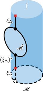
(a) $\vphantom{\biggl{(}}J_{\Delta\otimes{}\mathchoice{\leavevmode\hbox to6.3pt{\vbox to4.3pt{\text{[drawing]}}}}{\leavevmode\hbox to6.3pt{\vbox to4.3pt{\text{[drawing]}}}}{\leavevmode\hbox to3.67pt{\vbox to3.01pt{\text{[drawing]}}}}{\leavevmode\hbox to2.63pt{\vbox to2.15pt{\text{[drawing]}}}}^{*}}^{1/2}\otimes J_{\mathchoice{\leavevmode\hbox to6.3pt{\vbox to4.3pt{\text{[drawing]}}}}{\leavevmode\hbox to6.3pt{\vbox to4.3pt{\text{[drawing]}}}}{\leavevmode\hbox to3.67pt{\vbox to3.01pt{\text{[drawing]}}}}{\leavevmode\hbox to2.63pt{\vbox to2.15pt{\text{[drawing]}}}}}$, where $J_{\Delta}=\xi_{\Delta}\cdot\mathscr{M}$

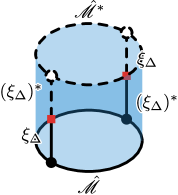
(b) $\vphantom{\biggl{(}}J_{\mathchoice{\leavevmode\hbox to6.3pt{\vbox to4.3pt{\text{[drawing]}}}}{\leavevmode\hbox to6.3pt{\vbox to4.3pt{\text{[drawing]}}}}{\leavevmode\hbox to3.67pt{\vbox to3.01pt{\text{[drawing]}}}}{\leavevmode\hbox to2.63pt{\vbox to2.15pt{\text{[drawing]}}}}\otimes\mathchoice{\leavevmode\hbox to6.3pt{\vbox to4.3pt{\text{[drawing]}}}}{\leavevmode\hbox to6.3pt{\vbox to4.3pt{\text{[drawing]}}}}{\leavevmode\hbox to3.67pt{\vbox to3.01pt{\text{[drawing]}}}}{\leavevmode\hbox to2.63pt{\vbox to2.15pt{\text{[drawing]}}}}^{*}}=J_{\mathchoice{\leavevmode\hbox to6.3pt{\vbox to4.3pt{\text{[drawing]}}}}{\leavevmode\hbox to6.3pt{\vbox to4.3pt{\text{[drawing]}}}}{\leavevmode\hbox to3.67pt{\vbox to3.01pt{\text{[drawing]}}}}{\leavevmode\hbox to2.63pt{\vbox to2.15pt{\text{[drawing]}}}}\otimes{}\mathchoice{\leavevmode\hbox to6.3pt{\vbox to4.3pt{\text{[drawing]}}}}{\leavevmode\hbox to6.3pt{\vbox to4.3pt{\text{[drawing]}}}}{\leavevmode\hbox to3.67pt{\vbox to3.01pt{\text{[drawing]}}}}{\leavevmode\hbox to2.63pt{\vbox to2.15pt{\text{[drawing]}}}}^{*}}^{1/2}\otimes J_{\mathchoice{\leavevmode\hbox to6.3pt{\vbox to4.3pt{\text{[drawing]}}}}{\leavevmode\hbox to6.3pt{\vbox to4.3pt{\text{[drawing]}}}}{\leavevmode\hbox to3.67pt{\vbox to3.01pt{\text{[drawing]}}}}{\leavevmode\hbox to2.63pt{\vbox to2.15pt{\text{[drawing]}}}}\otimes{}\mathchoice{\leavevmode\hbox to6.3pt{\vbox to4.3pt{\text{[drawing]}}}}{\leavevmode\hbox to6.3pt{\vbox to4.3pt{\text{[drawing]}}}}{\leavevmode\hbox to3.67pt{\vbox to3.01pt{\text{[drawing]}}}}{\leavevmode\hbox to2.63pt{\vbox to2.15pt{\text{[drawing]}}}}^{*}}^{1/2}$

Figure 5: A partial source $J_{\Delta\otimes{}\Delta^{*}}^{1/2}=\xi_{\Delta}\cdot\hat{\mathscr{M}}\cdot(\xi_{\Delta})^{*}$ (solid black), shown in each panel glued to another partial source (dashed black). A (part of a) possible bulk configuration that might appear in the path integral involving each of these glued partial sources is illustrated in blue.

At any rate, let us now instead consider the bounds 89 and 98 for a different partial source $J_{\Delta\otimes{}\Delta^{*}}^{1/2}$. Looking to side step the ambiguities raised above, we will choose a partial source whose gluing rules are already determined by close analogy to those of $\xi_{\Delta}\cdot\mathscr{M}$. We will see that eqs. 89 and 98 in this case are consistent with the typical dimension $\sim e^{2S_{0}}$ of $\mathcal{H}_{\Delta}^{\alpha}$ found in ref. Abdalla:2025gzn .

Let us denote the new partial sources we wish to consider by

$$J_{\Delta\otimes{}\Delta^{*}}^{1/2} =\xi_{\Delta}\cdot\hat{\mathscr{M}}\cdot(\xi_{\Delta})^{*}\in\mathcal{J}_{\Delta\otimes\Delta^{*}}\;,$$ (110)

$$J_{\Delta\otimes\Delta^{*}} =J_{\Delta\otimes{}\mathchoice{\leavevmode\hbox to6.57pt{\vbox to4.78pt{\text{[drawing]}}}}{\leavevmode\hbox to6.57pt{\vbox to4.78pt{\text{[drawing]}}}}{\leavevmode\hbox to4.08pt{\vbox to3.35pt{\text{[drawing]}}}}{\leavevmode\hbox to2.92pt{\vbox to2.39pt{\text{[drawing]}}}}^{*}}^{1/2}\otimes J_{\mathchoice{\leavevmode\hbox to6.57pt{\vbox to4.78pt{\text{[drawing]}}}}{\leavevmode\hbox to6.57pt{\vbox to4.78pt{\text{[drawing]}}}}{\leavevmode\hbox to4.08pt{\vbox to3.35pt{\text{[drawing]}}}}{\leavevmode\hbox to2.92pt{\vbox to2.39pt{\text{[drawing]}}}}\otimes{}\Delta^{*}}^{1/2}=\xi_{\Delta}\cdot\hat{\mathscr{M}}\cdot\gamma^{(\Delta)}\cdot\hat{\mathscr{M}}\cdot(\xi_{\Delta})^{*}\in\mathcal{J}_{\Delta\otimes\Delta^{*}}\;.\leavevmode\hbox to0pt{\vbox to0pt{\text{[drawing]}}} \scriptstyle\Delta \scriptstyle\Delta$$ (111)

As illustrated in fig. 5, $\xi_{\Delta}\cdot\hat{\mathscr{M}}\cdot(\xi_{\Delta})^{*}$ consists of two half worldlines $\xi_{\Delta}$ and $(\xi_{\Delta})^{*}$ for the observer, attached to an asymptotic boundary manifold $\hat{\mathscr{M}}$. We will require $\hat{\mathscr{M}}$ to be real in the sense that $J_{\Delta\otimes{}\Delta^{*}}^{1/2}$ satisfies eq. 87. The rules for gluing the half worldlines in this partial source to other half worldlines are what one expects from generalizing eq. 104 in the obvious way. For example, fig. 5(a) illustrates the gluing relevant for

$$O\left(\xi_{\Delta}\cdot\hat{\mathscr{M}}\cdot(\xi_{\Delta})^{*}\right)\ket{\xi_{\Delta}\cdot\mathscr{M},\alpha} =\ket{\xi_{\Delta}\cdot\hat{\mathscr{M}}\cdot\gamma^{(\Delta)}\cdot\mathscr{M},\alpha}$$ (112)

while fig. 5(b) illustrates the complete source

$$J_{\mathchoice{\leavevmode\hbox to6.57pt{\vbox to4.78pt{\text{[drawing]}}}}{\leavevmode\hbox to6.57pt{\vbox to4.78pt{\text{[drawing]}}}}{\leavevmode\hbox to4.08pt{\vbox to3.35pt{\text{[drawing]}}}}{\leavevmode\hbox to2.92pt{\vbox to2.39pt{\text{[drawing]}}}}\otimes\mathchoice{\leavevmode\hbox to6.57pt{\vbox to4.78pt{\text{[drawing]}}}}{\leavevmode\hbox to6.57pt{\vbox to4.78pt{\text{[drawing]}}}}{\leavevmode\hbox to4.08pt{\vbox to3.35pt{\text{[drawing]}}}}{\leavevmode\hbox to2.92pt{\vbox to2.39pt{\text{[drawing]}}}}^{*}} \scriptstyle\Delta \scriptstyle\Delta =J_{\mathchoice{\leavevmode\hbox to6.57pt{\vbox to4.78pt{\text{[drawing]}}}}{\leavevmode\hbox to6.57pt{\vbox to4.78pt{\text{[drawing]}}}}{\leavevmode\hbox to4.08pt{\vbox to3.35pt{\text{[drawing]}}}}{\leavevmode\hbox to2.92pt{\vbox to2.39pt{\text{[drawing]}}}}\otimes{}\mathchoice{\leavevmode\hbox to6.57pt{\vbox to4.78pt{\text{[drawing]}}}}{\leavevmode\hbox to6.57pt{\vbox to4.78pt{\text{[drawing]}}}}{\leavevmode\hbox to4.08pt{\vbox to3.35pt{\text{[drawing]}}}}{\leavevmode\hbox to2.92pt{\vbox to2.39pt{\text{[drawing]}}}}^{*}}^{1/2}\otimes J_{\mathchoice{\leavevmode\hbox to6.57pt{\vbox to4.78pt{\text{[drawing]}}}}{\leavevmode\hbox to6.57pt{\vbox to4.78pt{\text{[drawing]}}}}{\leavevmode\hbox to4.08pt{\vbox to3.35pt{\text{[drawing]}}}}{\leavevmode\hbox to2.92pt{\vbox to2.39pt{\text{[drawing]}}}}\otimes{}\mathchoice{\leavevmode\hbox to6.57pt{\vbox to4.78pt{\text{[drawing]}}}}{\leavevmode\hbox to6.57pt{\vbox to4.78pt{\text{[drawing]}}}}{\leavevmode\hbox to4.08pt{\vbox to3.35pt{\text{[drawing]}}}}{\leavevmode\hbox to2.92pt{\vbox to2.39pt{\text{[drawing]}}}}^{*}}^{1/2}=\vphantom{\Big{(}}\xi_{\mathchoice{\leavevmode\hbox to6.57pt{\vbox to4.78pt{\text{[drawing]}}}}{\leavevmode\hbox to6.57pt{\vbox to4.78pt{\text{[drawing]}}}}{\leavevmode\hbox to4.08pt{\vbox to3.35pt{\text{[drawing]}}}}{\leavevmode\hbox to2.92pt{\vbox to2.39pt{\text{[drawing]}}}}}\cdot\hat{\mathscr{M}}\cdot\gamma^{(\Delta)}\cdot\hat{\mathscr{M}}\cdot(\xi_{\mathchoice{\leavevmode\hbox to6.57pt{\vbox to4.78pt{\text{[drawing]}}}}{\leavevmode\hbox to6.57pt{\vbox to4.78pt{\text{[drawing]}}}}{\leavevmode\hbox to4.08pt{\vbox to3.35pt{\text{[drawing]}}}}{\leavevmode\hbox to2.92pt{\vbox to2.39pt{\text{[drawing]}}}}})^{*}\leavevmode\hbox to0pt{\vbox to0pt{\text{[drawing]}}} \scriptstyle\Delta \scriptstyle\Delta \scriptstyle\Delta \scriptstyle\Delta \scriptstyle\Delta \scriptstyle\Delta$$ (113)

for the path integrals appearing in eqs. 89 and 98.

To use eq. 98 to roughly bound the number of states in $\mathcal{H}_{\Delta}^{\alpha}$, we make the following three observations. Firstly, the topological suppression of bulk spacetimes of genus $g$ with $n$ boundaries goes like $\sim e^{S_{0}(2-2g-n)}$. Secondly, gluing $J_{\Delta\otimes\Delta^{*}}^{1/2}$ given in eq. 110 to a partial source $J_{\Delta}\in\mathcal{J}_{\Delta}$, viewed as preparing a state, effectively introduces an extra asymptotic boundary to the component of the bulk connected to $J_{\Delta}$. This is illustrated in fig. 5(a). Therefore, we expect typical eigenvalues of $O\left(J_{\Delta\otimes\Delta^{*}}\right)$, in the sense of dominating the LHS of eq. 98, to be of size $\sim(e^{-S_{0}})^{2}$. Thirdly, the path integral $\zeta\Big{(}J_{\mathchoice{\leavevmode\hbox to6.23pt{\vbox to4.78pt{\text{[drawing]}}}}{\leavevmode\hbox to6.23pt{\vbox to4.78pt{\text{[drawing]}}}}{\leavevmode\hbox to3.85pt{\vbox to3.35pt{\text{[drawing]}}}}{\leavevmode\hbox to2.75pt{\vbox to2.39pt{\text{[drawing]}}}}\otimes\mathchoice{\leavevmode\hbox to6.23pt{\vbox to4.78pt{\text{[drawing]}}}}{\leavevmode\hbox to6.23pt{\vbox to4.78pt{\text{[drawing]}}}}{\leavevmode\hbox to3.85pt{\vbox to3.35pt{\text{[drawing]}}}}{\leavevmode\hbox to2.75pt{\vbox to2.39pt{\text{[drawing]}}}}^{*}}\Big{)}$ has a leading order contribution, in the topological expansion, whose connected bulk component is the cylinder illustrated in fig. 5(b). The contribution of this cylinder is $\sim(e^{S_{0}})^{0}$. Altogether, it follows that the ensemble-average number of eigenstates of $O\left(J_{\Delta\otimes\Delta^{*}}\right)$, in the window where eigenvalues are of the typical size $\sim{}e^{-2S_{0}}$ in eq. 98, is bounded by $\sim{}e^{2S_{0}}$. This is consistent with the finding of ref. Abdalla:2025gzn that the dimension of the gravitational Hilbert space with one observer is $\sim e^{2S_{0}}$.

In the above discussion, for simplicity, we have described observers with one internal state. In fact, refs. Maldacena:2024spf ; Abdalla:2025gzn consider observers with some number $d$ of orthogonal internal states $\sigma$, with different energies corresponding to different values of $\Delta$, such that a “clock” can be constructed from these states. It is straightforward to generalize to this case by taking a direct sum of the above discussion. That is, the sector $\mathcal{H}_{\sigma}^{\alpha}$ of the gravitational Hilbert space associated with each internal state $\sigma$ of an observer is just one instance of the $\sim e^{2S_{0}}$-dimensional $\mathcal{H}_{\Delta}^{\alpha}$ described above. The direct sum $\bigoplus_{\sigma=1}^{d}\mathcal{H}_{\sigma}^{\alpha}$ then gives the $\sim{}d\,e^{2S_{0}}$-dimensional gravitational Hilbert space with one observer.

5.2.2 External observer clones

Next, let us see how our framework applies to another prescription, by Harlow, Usatyuk, and Zhao Harlow:2025pvj , for evaluating the gravitational path integral in the presence of observers. Their proposal is to treat observers just like any other bulk matter excitation, except that the source preparing the state of the observer is “entangled” with a “clone” of the observer, modelled as an external non-gravitational system.

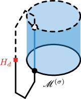
(a) A partial source $\tilde{J}_{d}=\sum_{\sigma=1}^{d}\mathscr{M}^{(\sigma)}\ket{\sigma}\in\tilde{\mathcal{J}}_{d}$ where $\mathscr{M}^{(\sigma)}$ is required to excite an observer in state $\sigma$.

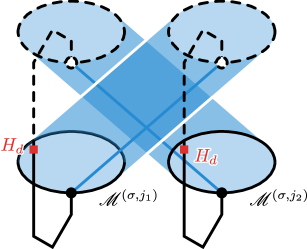
(b) $\tilde{J}_{d}^{(j_{1})}\otimes\tilde{J}_{d}^{(j_{2})}$ for $\tilde{J}_{d}^{(j_{1})}=\sum_{\sigma=1}^{d}\mathscr{M}^{(\sigma,j_{1})}\ket{\sigma}\in\tilde{\mathcal{J}}_{d}$ and similarly $\tilde{J}_{d}^{(j_{2})}\in\tilde{\mathcal{J}}_{d}$.

Figure 6: Partial sources $\tilde{J}_{d}\in\tilde{\mathcal{J}}_{d}$ and $\tilde{J}_{d}^{(j_{1})}\otimes\tilde{J}_{d}^{(j_{2})}\in\tilde{\mathcal{J}}_{d}\otimes\tilde{\mathcal{J}}_{d}$ (solid black). We also illustrate $(\tilde{J}_{d}^{\prime}|\tilde{J}_{d}),(\tilde{J}_{d}^{(i_{1})}\otimes\tilde{J}_{d}^{(i_{2})}|\tilde{J}_{d}^{(j_{1})}\otimes\tilde{J}_{d}^{(j_{2})})\in\mathcal{J}$ for some $\tilde{J}_{d}^{\prime},\tilde{J}_{d}^{(i_{1})},\tilde{J}_{d}^{(i_{2})}\in\tilde{\mathcal{J}}_{d}$ (dashed black). A possible bulk configuration that might appear in the path integral $\zeta$ evaluated with each complete source is illustrated in blue.

Here, the set $\mathcal{J}$ of complete sources for the path integral is generated just by boundary manifolds $\mathscr{M}$ preparing states of closed universes. To introduce the observer and its clone, ref. Harlow:2025pvj considers, in our language, a set $\tilde{\mathcal{J}}_{d}$ of partial sources which is a submodule of the $\mathcal{J}_{d}$ introduced in eq. 34. In particular,

$$\tilde{\mathcal{J}}_{d}=\operatorname{span}\left\{\sum_{\sigma=1}^{d}\mathscr{M}^{(\sigma)}\ket{\sigma}:\text{boundary manifold $\mathscr{M}^{(\sigma)}\in\mathcal{J}$ excites observer in state $\sigma$}\right\}$$ (114)

where $\mathscr{M}^{(\sigma)}$ is a boundary manifold preparing an arbitrary state of closed universes, including excitations of at least some matter constituting one observer in an internal state labelled by $\sigma$. In the two-dimensional topological Marolf:2020xie and JT models for which ref. Harlow:2025pvj performed explicit calculations, the observer is simply modelled as a matter worldline of flavour $\sigma$. The superposition in eq. 114 indicates the sense in which the internal state of this bulk observer is entangled with the state $\ket{\sigma}$ of an external clone. Because $\tilde{\mathcal{J}}_{d}$ is a submodule of $\mathcal{J}_{d}$, it naturally inherits the gluing operation 37 and Hermitian form 35. In fig. 6(a), we illustrate a partial source $\tilde{J}_{d}\in\tilde{\mathcal{J}}_{d}$ and its gluing to another partial source $(\tilde{J}_{d}^{\prime})^{*}\in\tilde{\mathcal{J}}_{d^{*}}$.

From $\tilde{\mathcal{J}}_{d}$, we can define $\alpha$-sector Hilbert spaces $\tilde{\mathcal{H}}_{d}^{\alpha}$ as described in section 3.3. Analogous to eq. 105, a path integral with insertions of $\tilde{J}_{d}^{(j_{1})},\ldots,\tilde{J}_{d}^{(j_{n})}\in\tilde{\mathcal{J}}_{d}$ glued to the $*$-conjugates of $\tilde{J}_{d}^{(i_{1})},\ldots,\tilde{J}_{d}^{(i_{n})}\in\tilde{\mathcal{J}}_{d}$,

$$\begin{split}&\zeta\left((\tilde{J}_{d}^{(i_{1})}|\tilde{J}_{d}^{(j_{1})})\sqcup\cdots\sqcup(\tilde{J}_{d}^{(i_{n})}|\tilde{J}_{d}^{(j_{n})})\right)\\ &=\int_{\mathcal{A}}\differential{\alpha}\absolutevalue{\innerproduct{\alpha}{\varnothing}}^{2}\tensor[_{\mathrm{r}}]{\innerproduct{\tilde{J}_{d}^{(i_{1})},\alpha}{\tilde{J}_{d}^{(j_{1})},\alpha}}{{}_{\mathrm{r}}}\cdots\tensor[_{\mathrm{r}}]{\innerproduct{\tilde{J}_{d}^{(i_{n})},\alpha}{\tilde{J}_{d}^{(j_{n})},\alpha}}{{}_{\mathrm{r}}}\;,\end{split}$$ (115)

gives moments of the $\alpha$-sector $\tilde{\mathcal{H}}_{d}^{\alpha}$ inner products $\tensor[_{\mathrm{r}}]{\innerproduct{\tilde{J}_{d}^{(i)},\alpha}{\tilde{J}_{d}^{(j)},\alpha}}{{}_{\mathrm{r}}}$ in the Hartle-Hawking ensemble. Note that, unlike the prescription of ref. Abdalla:2025gzn described in section 5.2.1, the bulk observer worldline is not prescribed to connect certain bra- pieces of the boundary manifold to certain ket- pieces — see fig. 6(b) for an example of a bulk configuration that can contribute to the above path integral for $n=2$.

Evaluating path integrals like eq. 115 in a two-dimensional model of topological gravity Marolf:2020xie and in AdS JT gravity, the analysis of ref. Harlow:2025pvj can be understood as approximating the typical rank of the Gram matrix $\tensor[_{\mathrm{r}}]{\innerproduct{\tilde{J}_{d}^{(i)},\alpha}{\tilde{J}_{d}^{(j)},\alpha}}{{}_{\mathrm{r}}}$. Their result, that $\tilde{\mathcal{H}}_{d}^{\alpha}$ can have dimension greater than one, is again unsurprising from our general analysis in section 3.3. Again, we can use our general bound 89 and its ensemble average 98 to roughly constrain the size of $\tilde{\mathcal{H}}_{d}^{\alpha}$, finding agreement below with the quantitative results of ref. Harlow:2025pvj .

In preparation, let us first argue that

$$\dim\tilde{\mathcal{H}}_{d}^{\alpha}\leq\dim\mathcal{H}_{d}^{\alpha}=d\;,$$ (116)

where $\mathcal{H}_{d}^{\alpha}$ is the $\alpha$-sector Hilbert space constructed from the set $\mathcal{J}_{d}$ of partial sources defined in eq. 34. The coefficients $J^{(\varsigma)}$ in eq. 34 are arbitrary elements of the set $\mathcal{J}$ of sources, so $\tilde{\mathcal{J}}_{d}$ defined in eq. 114 is clearly a submodule of $\mathcal{J}_{d}$. It then follows that $\tilde{\mathcal{H}}_{d}^{\alpha}$ is a subspace of $\mathcal{H}_{d}^{\alpha}$, hence the inequality in eq. 116. Next, we observe that $\mathcal{H}_{d}^{\alpha}$ is isometric to the $d$-dimensional Hilbert space $H_{d}$ of the external quantum mechanical system:

$$\mathcal{H}_{d}^{\alpha} \leftrightarrow H_{d}\;, \ket{\sum_{\varsigma=1}^{d}J^{(\varsigma)}\ket{\varsigma},\alpha}_{\mathrm{r}} \leftrightarrow\sum_{\varsigma=1}^{d}Z_{\alpha}(J^{(\varsigma)})\ket{\varsigma}\;.$$ (117)

For a closer analogy to our discussion in section 5.2.1, however, let us mention a more round-about derivation of the last equality in eq. 116. Let us consider the two-sided partial source

$$I_{d\otimes d^{*}} =\sum_{\varsigma=1}^{d}\outerproduct{\varsigma}{\varsigma}\in\mathcal{J}_{d\otimes d^{*}}\;.$$ (119)

This is the identity operator on $H_{d}$ and the corresponding $O(I_{d\otimes{}d^{*}})$, defined by eq. 73, is the identity operator on $\mathcal{H}_{d}^{\alpha}$. The condition 97 for the saturation of the bound 89 is manifestly satisfied by the expression 119 for $I_{d\otimes d^{*}}=I_{d\otimes d^{*}}^{1/2}$. The saturated bound then gives

$$\dim\mathcal{H}_{d}^{\alpha} =Z_{\alpha}\Big{(}I_{\mathchoice{\leavevmode\hbox to4.16pt{\vbox to4.86pt{\text{[drawing]}}}}{\leavevmode\hbox to4.16pt{\vbox to4.86pt{\text{[drawing]}}}}{\leavevmode\hbox to2.55pt{\vbox to3.4pt{\text{[drawing]}}}}{\leavevmode\hbox to1.82pt{\vbox to2.43pt{\text{[drawing]}}}}\otimes\mathchoice{\leavevmode\hbox to4.16pt{\vbox to4.86pt{\text{[drawing]}}}}{\leavevmode\hbox to4.16pt{\vbox to4.86pt{\text{[drawing]}}}}{\leavevmode\hbox to2.55pt{\vbox to3.4pt{\text{[drawing]}}}}{\leavevmode\hbox to1.82pt{\vbox to2.43pt{\text{[drawing]}}}}^{*}}\Big{)}=d\,Z_{\alpha}(\varnothing)=d\;,\leavevmode\hbox to0pt{\vbox to0pt{\text{[drawing]}}} \scriptstyle d \scriptstyle d$$ (120)

as desired.

We saw in section 5.2.1 that, by considering another two-sided partial source 111, the ensemble-averaged bound 98 gave a useful rough bound on the size of Hilbert space $\mathcal{H}_{\Delta}^{\alpha}$. Let us now demonstrate that a completely analogous construction leads to a rough bound on the typical size of $\tilde{\mathcal{H}}_{d}^{\alpha}$ which is sometimes stronger than eq. 116 and roughly saturated by the results of Harlow:2015lma . The analogous partial sources in the present context would be

$$\tilde{J}_{d\otimes{}d^{*}}^{1/2} =\sum_{\sigma,\sigma^{\prime}=1}^{d}\hat{\mathscr{M}}^{(\sigma,\sigma^{\prime})}\outerproduct{\sigma}{\sigma^{\prime}}\in\tilde{\mathcal{J}}_{d\otimes{}d^{*}}\;,$$ (122)

$$J_{d\otimes d^{*}} =J_{d\otimes{}\mathchoice{\leavevmode\hbox to4.16pt{\vbox to4.86pt{\text{[drawing]}}}}{\leavevmode\hbox to4.16pt{\vbox to4.86pt{\text{[drawing]}}}}{\leavevmode\hbox to2.55pt{\vbox to3.4pt{\text{[drawing]}}}}{\leavevmode\hbox to1.82pt{\vbox to2.43pt{\text{[drawing]}}}}^{*}}^{1/2}\otimes J_{\mathchoice{\leavevmode\hbox to4.16pt{\vbox to4.86pt{\text{[drawing]}}}}{\leavevmode\hbox to4.16pt{\vbox to4.86pt{\text{[drawing]}}}}{\leavevmode\hbox to2.55pt{\vbox to3.4pt{\text{[drawing]}}}}{\leavevmode\hbox to1.82pt{\vbox to2.43pt{\text{[drawing]}}}}\otimes{}d^{*}}^{1/2}=\sum_{\sigma,\sigma^{\prime},\sigma^{\prime\prime}=1}^{d}\hat{\mathscr{M}}^{(\sigma,\sigma^{\prime})}\sqcup\hat{\mathscr{M}}^{(\sigma^{\prime},\sigma^{\prime\prime})}\outerproduct{\sigma}{\sigma^{\prime\prime}}\in\tilde{\mathcal{J}}_{d\otimes{}d^{*}} \scriptstyle d \scriptstyle d$$ (123)

where $\hat{\mathscr{M}}^{(\sigma,\sigma^{\prime})}\in\mathcal{J}$ is a boundary manifold which excites at least an observer and an anti-observer in states $\sigma$ and $(\sigma^{\prime})^{*}$ respectively — see fig. 7. (Exciting an anti-observer in state $(\sigma^{\prime})^{*}$ is equivalent to absorbing an observer in state $\sigma^{\prime}$.) To ensure that $\tilde{J}_{d\otimes{}d^{*}}^{1/2}$ satisfies the reality condition 87, we will further require $\hat{\mathscr{M}}^{(\sigma,\sigma^{\prime})}$ to satisfy

$$\left(\hat{\mathscr{M}}^{(\sigma,\sigma^{\prime})}\right)^{*} =\hat{\mathscr{M}}^{(\sigma^{\prime},\sigma)}\;.$$ (124)

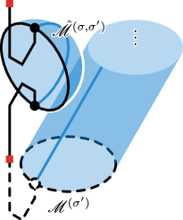
(a) Part of a bulk topology in a path integral involving $\vphantom{\biggl{(}}\tilde{J}_{d\otimes{}\mathchoice{\leavevmode\hbox to4.05pt{\vbox to4.38pt{\text{[drawing]}}}}{\leavevmode\hbox to4.05pt{\vbox to4.38pt{\text{[drawing]}}}}{\leavevmode\hbox to2.3pt{\vbox to3.06pt{\text{[drawing]}}}}{\leavevmode\hbox to1.64pt{\vbox to2.19pt{\text{[drawing]}}}}^{*}}^{1/2}\otimes\tilde{J}_{\mathchoice{\leavevmode\hbox to4.05pt{\vbox to4.38pt{\text{[drawing]}}}}{\leavevmode\hbox to4.05pt{\vbox to4.38pt{\text{[drawing]}}}}{\leavevmode\hbox to2.3pt{\vbox to3.06pt{\text{[drawing]}}}}{\leavevmode\hbox to1.64pt{\vbox to2.19pt{\text{[drawing]}}}}}=\sum_{\sigma,\sigma^{\prime}=1}^{d}\hat{\mathscr{M}}^{(\sigma,\sigma^{\prime})}\sqcup\mathscr{M}^{(\sigma^{\prime})}\ket{\sigma}$ where $\tilde{J}_{d}=\sum_{\sigma^{\prime}=1}^{d}\mathscr{M}^{(\sigma^{\prime})}\ket{\sigma^{\prime}}$. When $e^{2S_{0}}\gg d$, bulk topologies of this kind dominate the path integral.

(b) Part of another bulk topology in the path integral involving $\vphantom{\biggl{(}}\tilde{J}_{d\otimes{}\mathchoice{\leavevmode\hbox to4.05pt{\vbox to4.38pt{\text{[drawing]}}}}{\leavevmode\hbox to4.05pt{\vbox to4.38pt{\text{[drawing]}}}}{\leavevmode\hbox to2.3pt{\vbox to3.06pt{\text{[drawing]}}}}{\leavevmode\hbox to1.64pt{\vbox to2.19pt{\text{[drawing]}}}}^{*}}^{1/2}\otimes\tilde{J}_{\mathchoice{\leavevmode\hbox to4.05pt{\vbox to4.38pt{\text{[drawing]}}}}{\leavevmode\hbox to4.05pt{\vbox to4.38pt{\text{[drawing]}}}}{\leavevmode\hbox to2.3pt{\vbox to3.06pt{\text{[drawing]}}}}{\leavevmode\hbox to1.64pt{\vbox to2.19pt{\text{[drawing]}}}}}$. When $d\gg e^{2S_{0}}\gg 1$, bulk topologies connecting the boundary manifolds $\hat{\mathscr{M}}^{(\sigma,\sigma^{\prime})}$ and $\hat{\mathscr{M}}^{(\sigma^{\prime})}$ like this dominate the path integral.

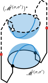
(c) A bulk topology in the path integral with the source $\vphantom{\bigg{(}}\tilde{J}_{\mathchoice{\leavevmode\hbox to4.05pt{\vbox to4.38pt{\text{[drawing]}}}}{\leavevmode\hbox to4.05pt{\vbox to4.38pt{\text{[drawing]}}}}{\leavevmode\hbox to2.3pt{\vbox to3.06pt{\text{[drawing]}}}}{\leavevmode\hbox to1.64pt{\vbox to2.19pt{\text{[drawing]}}}}\otimes\mathchoice{\leavevmode\hbox to4.05pt{\vbox to4.38pt{\text{[drawing]}}}}{\leavevmode\hbox to4.05pt{\vbox to4.38pt{\text{[drawing]}}}}{\leavevmode\hbox to2.3pt{\vbox to3.06pt{\text{[drawing]}}}}{\leavevmode\hbox to1.64pt{\vbox to2.19pt{\text{[drawing]}}}}^{*}}=\tilde{J}_{\mathchoice{\leavevmode\hbox to4.05pt{\vbox to4.38pt{\text{[drawing]}}}}{\leavevmode\hbox to4.05pt{\vbox to4.38pt{\text{[drawing]}}}}{\leavevmode\hbox to2.3pt{\vbox to3.06pt{\text{[drawing]}}}}{\leavevmode\hbox to1.64pt{\vbox to2.19pt{\text{[drawing]}}}}\otimes{}\mathchoice{\leavevmode\hbox to4.05pt{\vbox to4.38pt{\text{[drawing]}}}}{\leavevmode\hbox to4.05pt{\vbox to4.38pt{\text{[drawing]}}}}{\leavevmode\hbox to2.3pt{\vbox to3.06pt{\text{[drawing]}}}}{\leavevmode\hbox to1.64pt{\vbox to2.19pt{\text{[drawing]}}}}^{*}}^{1/2}\otimes\tilde{J}_{\mathchoice{\leavevmode\hbox to4.05pt{\vbox to4.38pt{\text{[drawing]}}}}{\leavevmode\hbox to4.05pt{\vbox to4.38pt{\text{[drawing]}}}}{\leavevmode\hbox to2.3pt{\vbox to3.06pt{\text{[drawing]}}}}{\leavevmode\hbox to1.64pt{\vbox to2.19pt{\text{[drawing]}}}}\otimes{}\mathchoice{\leavevmode\hbox to4.05pt{\vbox to4.38pt{\text{[drawing]}}}}{\leavevmode\hbox to4.05pt{\vbox to4.38pt{\text{[drawing]}}}}{\leavevmode\hbox to2.3pt{\vbox to3.06pt{\text{[drawing]}}}}{\leavevmode\hbox to1.64pt{\vbox to2.19pt{\text{[drawing]}}}}^{*}}^{1/2}=\sum_{\sigma,\sigma^{\prime}=1}^{d}\hat{\mathscr{M}}^{(\sigma,\sigma^{\prime})}\sqcup\hat{\mathscr{M}}^{(\sigma^{\prime},\sigma)}$. When $e^{2S_{0}}\gg d$, this bulk topology dominates the path integral.

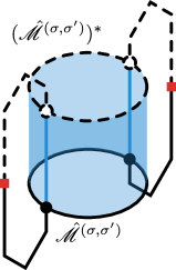
(d) Another bulk topology for the path integral with source $\vphantom{\biggl{(}}\tilde{J}_{\mathchoice{\leavevmode\hbox to4.05pt{\vbox to4.38pt{\text{[drawing]}}}}{\leavevmode\hbox to4.05pt{\vbox to4.38pt{\text{[drawing]}}}}{\leavevmode\hbox to2.3pt{\vbox to3.06pt{\text{[drawing]}}}}{\leavevmode\hbox to1.64pt{\vbox to2.19pt{\text{[drawing]}}}}\otimes\mathchoice{\leavevmode\hbox to4.05pt{\vbox to4.38pt{\text{[drawing]}}}}{\leavevmode\hbox to4.05pt{\vbox to4.38pt{\text{[drawing]}}}}{\leavevmode\hbox to2.3pt{\vbox to3.06pt{\text{[drawing]}}}}{\leavevmode\hbox to1.64pt{\vbox to2.19pt{\text{[drawing]}}}}^{*}}$. When $d\gg e^{2S_{0}}\gg 1$, this bulk topology dominates the path integral.

Figure 7: A partial source $\tilde{J}_{d\otimes d^{*}}^{1/2}=\sum_{\sigma,\sigma^{\prime}=1}^{d}\hat{\mathscr{M}}^{(\sigma,\sigma^{\prime})}\outerproduct{\sigma}{\sigma^{\prime}}$ (solid black), shown in each panel glued to another partial source (dashed black). A (part of a) possible bulk topology that might appear in the path integral involving each of these glued partial sources is illustrated in blue.

The reason why the trace of $O(\tilde{J}_{d\otimes d^{*}})$ is better suited for estimating the size of $\tilde{\mathcal{H}}_{d}^{\alpha}$ is because, unlike the identity operator $O(I_{d\otimes{}d^{*}})$ on $\mathcal{H}_{d}^{\alpha}$, the operator $O(\tilde{J}_{d\otimes d^{*}})$ projects $\mathcal{H}_{d}^{\alpha}\to\tilde{\mathcal{H}}_{d}^{\alpha}$. To use eq. 98 to roughly bound the number of states in $\tilde{\mathcal{H}}_{d}^{\alpha}$, we make the following three observations. Firstly, the topological suppression of bulk spacetimes of genus $g$ with $n$ boundaries goes like $\sim e^{S_{0}\,(2-2g-n)+S_{\partial}\,n}$ where $S_{\partial}=0$ in JT gravity and $S_{\partial}=S_{0}$ in the two-dimensional topological model of gravity Marolf:2020xie .

Secondly, let us consider the gluing of $\tilde{J}_{d\otimes{}d^{*}}^{1/2}$ given in eq. 122 to a partial source $\tilde{J}_{d}\in\tilde{\mathcal{J}}_{d}$ preparing a state, e.g. as illustrated in figs. 7(a) and 7(b). If $e^{S_{0}}\gg d$, then due to the strong topological suppression, we expect the leading order effect of attaching $\tilde{J}_{d\otimes{}d^{*}}^{1/2}$ to be the introduction of a disconnected disk with boundary $\hat{\mathscr{M}}^{(\sigma,\sigma^{\prime})}$ in the path integral, as illustrated in fig. 7(a). Therefore, we expect typical eigenvalues of $O(\tilde{J}_{d\otimes{}d^{*}})$, again in the sense of dominating the LHS of eq. 98, to be of size

$$\sim\left(e^{S_{0}+S_{\partial}}\right)^{2} \text{if $e^{2S_{0}}\gg d$}\;.$$ (125)

On the other hand, if $d\gg{}e^{S_{0}}\gg{}1$, then topologies which admit observer/clone loops become more favourable, with each loop contributing a factor of $\dim{H_{d}}=d$ — see fig. 7(b). Therefore, we expect typical eigenvalues of $O(\tilde{J}_{d\otimes{}d^{*}})$ to be of size

$$\sim\left(d\,e^{-S_{0}+S_{\partial}}\right)^{2} \text{if $d\gg e^{2S_{0}}\gg 1$}\;.$$ (126)

Thirdly, let us consider the path integral $\zeta\Big{(}\tilde{J}_{\mathchoice{\leavevmode\hbox to4.16pt{\vbox to4.86pt{\text{[drawing]}}}}{\leavevmode\hbox to4.16pt{\vbox to4.86pt{\text{[drawing]}}}}{\leavevmode\hbox to2.55pt{\vbox to3.4pt{\text{[drawing]}}}}{\leavevmode\hbox to1.82pt{\vbox to2.43pt{\text{[drawing]}}}}\otimes\mathchoice{\leavevmode\hbox to4.16pt{\vbox to4.86pt{\text{[drawing]}}}}{\leavevmode\hbox to4.16pt{\vbox to4.86pt{\text{[drawing]}}}}{\leavevmode\hbox to2.55pt{\vbox to3.4pt{\text{[drawing]}}}}{\leavevmode\hbox to1.82pt{\vbox to2.43pt{\text{[drawing]}}}}^{*}}\Big{)}$ appearing on the RHS of eq. 98. By similar reasoning as in the previous paragraph, after dividing out bulk components disconnected from the source, the dominant contribution to this path integral comes from two disks

$$\sim d\,(e^{S_{0}+S_{\partial}})^{2} \text{if $e^{2S_{0}}\gg d$},$$ (127)

as illustrated in fig. 7(c); or a cylinder

$$\sim{}d^{2}\,e^{2S_{\partial}} \text{if $d\gg e^{2S_{0}}\gg 1$}\;,$$ (128)

as illustrated in fig. 7(d).

Finally, let us suppose that a rough measure of the ensemble-averaged size of $\mathcal{H}_{d}^{\alpha}$ is given by the number of eigenstates of $O(\tilde{J}_{d\otimes{}d^{*}})$, in the window where eigenvalues are of the typical size 125 or 126. Then, using eqs. 127 and 128, we see that eq. 98 bounds this number of states from above by

$$\sim\min(d,e^{2S_{0}})\;.$$ (129)

In fact, ref. Harlow:2025pvj reports the ensemble-averaged dimension of $\mathcal{H}_{d}^{\alpha}$ to be $\sim\min(d,e^{2S_{0}})$.

5.3 Future directions

Let us conclude with some remarks on future directions for exploration.

In section 4.1, we introduced operators $O(J_{C\otimes{}C^{*}})$ which glue partial sources $J_{C\otimes{}C^{*}}$ to states in $\mathcal{H}_{C}^{\alpha}$. It is straightforward to extend this definition to two-sided Hilbert spaces $\mathcal{H}_{C\otimes C^{\prime}}^{\alpha}$. In close analogy to ref. Colafranceschi:2023moh , one might consider taking the completion of these operators in the weak operator topology to obtain a von Neumann algebra. Ref. Colafranceschi:2023moh focused on the case where $J_{C\otimes{}C^{*}}$ is a partial boundary manifold and $C=\Sigma$ is a cut of a boundary manifold. By studying the structure of the resulting von Neumann algebra $\mathcal{A}_{C}$, it was found that much can be learned about the structure of the Hilbert space on which the operators act. For example, two-sided Hilbert spaces decompose Colafranceschi:2023moh ; Marolf:2024adj

$$\mathcal{H}_{C\otimes C^{\prime}}^{\alpha} =\bigoplus_{\mu}\mathcal{H}_{C}^{\alpha,\mu}\otimes\mathcal{H}_{C^{\prime}}^{\alpha,\mu}$$ (130)

into factorizing eigenspaces of central elements of $\mathcal{A}_{C}$. It would be interesting to carry out an analogous analysis in the generalized framework of this paper, including abstract partial sources for the path integral. In particular, one might try to understand whether two-observer Hilbert spaces decompose in a similar manner as two-boundary Hilbert spaces do above. We might expect results analogous to refs. Colafranceschi:2023moh ; Marolf:2024adj since, at least superficially, almost all of their axioms (for each $\alpha$-sector path integral $\zeta_{\alpha}=Z_{\alpha}$) seem to have obvious analogues in the generalized framework considered in this paper, with the possible exception of their continuity axiom.

In section 5.2.1, we raised the possibility of interpreting path integrals with circular observer worldlines as partition functions counting states in the Hilbert space of closed universes with an observer. Again, there are several open questions here. Can we appropriately define the path integral so that it gives a positive (as opposed to complex Polchinski:1988ua or negative Maldacena:2024spf ) number? Would starting in Lorentzian signature help in this regard Casali:2021ewu ; Maldacena:2024spf ? One might think that JT gravity would be a simple model in which we can easily answer these questions. However, a naive Euclidean AdS JT path integral seems to undercount the number of closed universe states in the presence of an observer, as described in section 5.2.1, so we require a more sophisticated definition of the path integral with a circular observer worldline. Alternatively, one might ask what is the physical interpretation if it is instead the case that the partial sources required to construct circular observer worldlines cannot be included in AdS JT gravity while preserving the positivity of the gravitational inner product.

Finally, it would be interesting to explore the extent to which the gravitational path integral can be characterized as a random non-isometric code Akers:2022qdl ; Harlow:2025pvj ; Akers:2025ahe .

To make some concrete comments in this direction, let us consider the prescription of ref. Harlow:2025pvj described in section 5.2.2 for introducing external observer clones entangled with observers in closed universes. As we have described in section 5.2.2, in our language, partial sources $\tilde{J}_{d}\in\tilde{\mathcal{J}}_{d}$ prepare states $\ket{\tilde{J}_{d},\alpha}_{\mathrm{r}}$ in the $\alpha$-sector Hilbert space $\tilde{\mathcal{H}}_{d}^{\alpha}$ where an external observer clone is entangled with a bulk observer. Let us consider a family of such partial sources

$$\tilde{J}_{d}^{(i)} =\sum_{\sigma=1}^{d}\mathscr{M}^{(\sigma,i)}\ket{\sigma}\;,$$ (131)

where $\mathscr{M}^{(\sigma,i)}$ is a boundary manifold preparing a bulk observer in the state labelled by $\sigma$ and other bulk degrees of freedom in a semiclassical state labelled by $i$. The naive inner product $\innerproduct{i}{j}$ of perturbative semiclassical fields suggests a Hilbert space of arbitrarily large dimension — we will refer to this naive description as the “effective” description. In contrast, as described in section 5.2.2, each $\alpha$-sector Hilbert space $\tilde{\mathcal{H}}_{d}^{\alpha}$ of the full gravitational theory, with inner product $\tensor[_{\mathrm{r}}]{\innerproduct{\tilde{J}_{d}^{(i)},\alpha}{\tilde{J}_{d}^{(j)},\alpha}}{{}_{\mathrm{r}}}$, has bounded dimension. In particular, as described below eq. 116, $\tilde{\mathcal{H}}_{d}^{\alpha}$ is isometric to a subspace of the $d$-dimensional Hilbert space $H_{d}$ of the external observer clone.

Ref. Harlow:2025pvj describes their prescription as implementing a non-isometric code mapping states $\ket{i}$ in the effective description to a “fundamental” description by states in the Hilbert space $H_{d}$ of the external observer clone. With the aid of eq. 117, we see that this non-isometric map $V_{\alpha}$ (denoted $\hat{V}$ in ref. Harlow:2025pvj ) can be written as

$$V_{\alpha}\ket{i} =\sum_{\sigma=1}^{d}Z_{\alpha}(\mathscr{M}^{(\sigma,i)})\ket{\sigma}\in H_{d}\;,$$ (132)

such that

$$\matrixelement{i}{V_{\alpha}^{\dagger}V_{\alpha}}{j} =\tensor[_{\mathrm{r}}]{\innerproduct{\tilde{J}_{d}^{(i)},\alpha}{\tilde{J}_{d}^{(j)},\alpha}}{{}_{\mathrm{r}}}\;.$$ (133)

In particular, the matrix elements of $V_{\alpha}$ are given by the $\alpha$-sector path integrals

$$\matrixelement{\sigma}{V_{\alpha}}{i} =Z_{\alpha}(\mathscr{M}^{(\sigma,i)})\;.$$ (134)

From eq. 115, we further see that the path integral $\zeta$, without the restriction to an $\alpha$-sector, corresponds to an ensemble average over the non-isometric code $V_{\alpha}$,

$$\zeta\left((\tilde{J}_{d}^{(i_{1})}|\tilde{J}_{d}^{(j_{1})})\sqcup\cdots\sqcup(\tilde{J}_{d}^{(i_{n})}|\tilde{J}_{d}^{(j_{n})})\right) =\int_{\mathcal{A}}\differential{\alpha}\absolutevalue{\innerproduct{\alpha}{\varnothing}}^{2}\matrixelement{i_{1}}{V_{\alpha}^{\dagger}V_{\alpha}}{j_{1}}\cdots\matrixelement{i_{n}}{V_{\alpha}^{\dagger}V_{\alpha}}{j_{n}}\;.$$ (135)

In this sense, the path integral $\zeta$ corresponds to a random non-isometric code. Even in very simple toy models where the non-isometric code $V_{\alpha}$ is built from a handful of tensors and the ensemble average is taken as the Harr measure integral over the tensors, the ensemble average produces contractions between tensor legs which resemble bulk wormhole connections between source components Akers:2022qdl ; Harlow:2025pvj . Ref. Akers:2025ahe further incorporates locality into the encoding by considering non-isometric codes built from tensor networks, finding that such toy models can also reproduce some aspects of the prescription by ref. Abdalla:2025gzn , described in section 5.2.1, for including bulk observers with prescribed worldlines. It would be interesting to explore the extent to which we can push this apparent correspondence between gravitational path integrals and random non-isometric codes.

- (1) G. Penington, Entanglement Wedge Reconstruction and the Information Paradox, JHEP 09 (2020) 002 [1905.08255].
- (2) A. Almheiri, N. Engelhardt, D. Marolf and H. Maxfield, The entropy of bulk quantum fields and the entanglement wedge of an evaporating black hole, JHEP 12 (2019) 063 [1905.08762].
- (3) G. Penington, S.H. Shenker, D. Stanford and Z. Yang, Replica wormholes and the black hole interior, JHEP 03 (2022) 205 [1911.11977].
- (4) A. Almheiri, T. Hartman, J. Maldacena, E. Shaghoulian and A. Tajdini, Replica Wormholes and the Entropy of Hawking Radiation, JHEP 05 (2020) 013 [1911.12333].
- (5) D. Marolf and H. Maxfield, Transcending the ensemble: baby universes, spacetime wormholes, and the order and disorder of black hole information, JHEP 08 (2020) 044 [2002.08950].
- (6) D. Marolf and H. Maxfield, Observations of Hawking radiation: the Page curve and baby universes, JHEP 04 (2021) 272 [2010.06602].
- (7) S.R. Coleman, Black holes as red herrings: Topological fluctuations and the loss of quantum coherence, Nucl. Phys. B 307 (1988) 867.
- (8) S.B. Giddings and A. Strominger, Loss of incoherence and determination of coupling constants in quantum gravity, Nucl. Phys. B 307 (1988) 854.
- (9) S.B. Giddings and A. Strominger, Baby Universes, Third Quantization and the Cosmological Constant, Nucl. Phys. B 321 (1989) 481.
- (10) M. Usatyuk, Z.-Y. Wang and Y. Zhao, Closed universes in two dimensional gravity, SciPost Phys. 17 (2024) 051 [2402.00098].
- (11) M. Usatyuk and Y. Zhao, Closed universes, factorization, and ensemble averaging, JHEP 02 (2025) 052 [2403.13047].
- (12) C. Akers, N. Engelhardt, D. Harlow, G. Penington and S. Vardhan, The black hole interior from non-isometric codes and complexity, JHEP 06 (2024) 155 [2207.06536].
- (13) D. Harlow, M. Usatyuk and Y. Zhao, Quantum mechanics and observers for gravity in a closed universe, 2501.02359.
- (14) C. Akers, G. Bueller, O. DeWolfe, K. Higginbotham, J. Reinking and R. Rodriguez, On observers in holographic maps, 2503.09681.
- (15) A.I. Abdalla, S. Antonini, L.V. Iliesiu and A. Levine, The gravitational path integral from an observer’s point of view, 2501.02632.
- (16) E. Colafranceschi, X. Dong, D. Marolf and Z. Wang, Algebras and Hilbert spaces from gravitational path integrals. Understanding Ryu-Takayanagi/HRT as entropy without AdS/CFT, JHEP 10 (2024) 063 [2310.02189].
- (17) J. McNamara and C. Vafa, Baby Universes, Holography, and the Swampland, 2004.06738.
- (18) D. Harlow, Wormholes, Emergent Gauge Fields, and the Weak Gravity Conjecture, JHEP 01 (2016) 122 [1510.07911].
- (19) J. Maldacena, Real observers solving imaginary problems, 2412.14014.
- (20) E. Witten, Bras and Kets in Euclidean Path Integrals, 2503.12771.
- (21) D. Marolf, On the nature of ensembles from gravitational path integrals, J. Phys. A 58 (2025) 035204 [2407.04625].
- (22) A. Blommaert, L.V. Iliesiu and J. Kruthoff, Gravity factorized, JHEP 09 (2022) 080 [2111.07863].
- (23) A. Blommaert, L.V. Iliesiu and J. Kruthoff, Alpha states demystified — towards microscopic models of AdS2 holography, JHEP 08 (2022) 071 [2203.07384].
- (24) D. Marolf and D. Zhang, When left and right disagree: entropy and von Neumann algebras in quantum gravity with general AlAdS boundary conditions, JHEP 08 (2024) 010 [2402.09691].
- (25) G.W. Gibbons and S.W. Hawking, Action Integrals and Partition Functions in Quantum Gravity, Phys. Rev. D 15 (1977) 2752.
- (26) G. Lin and M. Usatyuk, Revisiting the second order formalism of JT gravity, 2310.16081.
- (27) J. Polchinski, The phase of the sum over spheres, Phys. Lett. B 219 (1989) 251.
- (28) E. Casali, D. Marolf, H. Maxfield and M. Rangamani, Baby universes and worldline field theories, Class. Quant. Grav. 39 (2022) 134004 [2101.12221].