Readout sweet spots for spin qubits with strong spin-orbit interaction
Abstract
Qubit readout schemes often deviate from ideal projective measurements, introducing critical issues that limit quantum computing performance. In this work, we model charge-sensing-based readout for semiconductor spin qubits in double quantum dots, and identify key error mechanisms caused by the back-action of the charge sensor. We quantify how the charge noise of the sensor, residual tunneling, and -tensor modulation degrade readout fidelity, induce a mixed post-measurement state, and cause leakage from the computational subspace. For state-of-the-art systems with strong spin-orbit interaction and electrically tunable -tensors, we identify a readout sweet spot, that is, a special device configuration where readout is closest to projective. Our framework provides a foundation for developing effective readout error mitigation strategies, with broad applications for optimizing readout performance for a variety of charge-sensing techniques, advancing quantum protocols, and improving adaptive circuits for error correction.
Introduction. Spin qubits confined in semiconductor quantum dots Loss and DiVincenzo (1998) are front-runners for large-scale quantum computers Hanson et al. (2007); Zwanenburg et al. (2013); Eriksson et al. (2004); Burkard et al. (2023); Wang et al. (2024); Zhang et al. (2025a); Philips et al. (2022); Hendrickx et al. (2021). Their small size, scalability Burkard et al. (2023); Kloeffel and Loss (2013); Vandersypen et al. (2017); Scappucci et al. (2021); Stano and Loss (2022), tunability, compatibility with CMOS technology Maurand et al. (2016); Xue et al. (2021); Jirovec et al. (2021); Liles et al. (2024); Camenzind et al. (2022); Zwerver et al. (2022); Neyens et al. (2024); Geyer et al. (2024); Steinacker et al. (2024), the demonstrated high-fidelity operations Xue et al. (2022); Noiri et al. (2022); Mills et al. (2022) and readout Takeda et al. (2024) make them particularly attractive.
A key component of quantum computers is readout, and an essential metric to quantify the quality of readout is its fidelity. However, while state-of-the-art experiments have demonstrated increasingly high fidelities Harvey-Collard et al. (2018); Blumoff et al. (2022); Nurizzo et al. (2023); Steinacker et al. (2024); Vigneau et al. (2023), this is not the only relevant benchmark Pereira et al. (2022, 2023). In fact, improving other metrics of mid-circuit measurements Rudinger et al. (2022); Zhang et al. (2025b); Hines and Proctor (2025); Hothem et al. (2024); McLaren et al. (2025), such as the quality of the post-measurement state, and readout-induced leakage from the computational subspace Miao et al. (2023); McEwen et al. (2021); Battistel et al. (2021); Marques et al. (2023), are key requirements for quantum error correction Liepelt et al. (2024); Gehér et al. (2024) and other powerful dynamic circuits. Tornow et al. (2022); Bäumer et al. (2024); Fleury et al. (2024); Stenger et al. (2025); Bäumer et al. (2024); Cao and Eisert (2025)
In this work, we present ways to simultaneously improve different metrics of state-of-the-art spin qubit readout. Our model focuses on widely-used measurements via Pauli blockade spin-to-charge conversion Ono et al. (2002); Petta et al. (2005); Koppens et al. (2006) and charge sensing in a double quantum dot (DQD) Haldar et al. (2025); Taubert et al. (2008); Ferguson et al. (2020); Young and Clerk (2010). By developing an intuitive microscopic model of charge sensing via a DC-biased quantum point contact (QPC) Elzerman et al. (2003, 2004); Gustavsson et al. (2006) - which can be straightforwardly generalized to multiple cases - we show that high-fidelity and back-action-free readout requires switching off the tunnel coupling between the dots upon charge sensing.
In current devices with strong spin-orbit interaction (e.g., holes in Ge and Si), the fluctuating electric field induced by the carriers of the QPC modulates the g-tensors of the spins in the DQD. We show that this modulation influences the quality of the readout, and this influence depends on the static homogeneous magnetic field applied to the DQD. We identify a readout sweet spot, i.e., a specific device configuration where the detrimental back-action effects of the g-tensor modulation are minimized: leakage is suppressed and the purity of the post-measurement state is maintained. We argue that this readout sweet spot exists universally, irrespectively from the details of spin-orbit interaction. Our findings provide practical guidelines for high-quality readout in spin-based quantum processors.
Model. To describe the readout of a qubit defined in a DQD, we rely on the general framework of quantum measurements, where the system is measured indirectly through a meter Wiseman and Milburn (2009); Diosi (2007). Simplifying earlier approaches to this problem Goan et al. (2001); Goan and Milburn (2001), we use a model in which the meter (the QPC) is also represented by a qubit, hence we call it the qubit measures qubit (QMQ) model. To illustrate the harmful effect of residual tunneling in the DQD, we apply this model to describe the readout of a charge qubit. Then, we generalize the QMQ model to the readout of spin qubits, where a residual tunneling has similar negative effects.
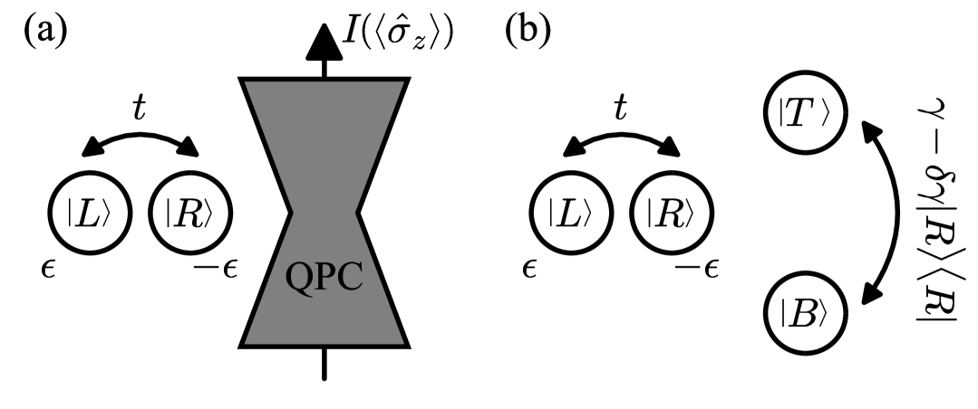
We consider the setup shown in Fig. 1a. The charge qubit is formed by a single carrier in the DQD; the qubit basis states and correspond to its position. The QPC current is high (low) if the DQD charge is in the left (right) dot, due to Coulomb repulsion between the DQD charge and the charges flowing through the QPC. In our QMQ model, the QPC is also represented by a single-carrier DQD, see Fig. 1b, with basis states corresponding to the bottom () and top () dots.
The Hamiltonian of the qubit-meter system reads
| (1) |
where , , , , and . Furthermore, is the on-site energy detuning, is the tunneling amplitude of the qubit, is the tunneling amplitude of the meter, and the interaction strength describes the Coulomb repulsion between the qubit and the meter.
One way to operate the charge qubit Petersson et al. (2010); Scarlino et al. (2022) is to perform coherent control at and , and sweep and to a readout point with Meinersen et al. (2024). Then, readout in the basis of the ground and excited states (at the readout point) is carried out by measuring the QPC current and inferring binary value or from the current trace.
In the QMQ model, readout of a qubit state is described as a sequence of indirect measurements, each consisting of three steps: (1) The meter is initialized in state . This state represents an electron approaching the QPC from the bottom lead. (2) The qubit-meter system evolves unitarily according to for time , entangling data and meter qubits via the interaction . The meter’s tunneling rate and the timestep are set such that by time , the transition probability to state is in an equal superposition or mixture of and . This corresponds to a QPC tuned to its charge-sensing working point where its conductance is of the conductance quantum. (3) The meter is measured projectively in the basis. The assigned measurement outcome is the number of transmitted electrons, i.e., 0 (1) if the QPC electron is found in the bottom (top) dot.
The number of these subsequent indirect measurements corresponds to the number of electrons that attempt to transit the QPC during readout. The current flowing through the QPC is represented as an -long bitstring, which contains 1-s where the QPC electron was transmitted. The state of the qubit is inferred from the transmission ratio using the maximum-likelihood principle, where is the number of electrons transmitted. That is, we infer if the probability of obtaining the measured transmission ratio is greater for the initial state then for ; we infer otherwise.
Measurement and back-action. The quantum channels corresponding to the final outcomes and are represented by superoperators and . They are called measurement operations Wiseman and Milburn (2009), and they map the pre-measurement state to the unnormalized post-measurement state conditional on the outcome. In the QMQ model, these measurement operations can be efficiently computed numerically (see SM S1.5 Hashim et al. (2024)). Since and completely characterize the measurement, we extract all relevant readout metrics from them.
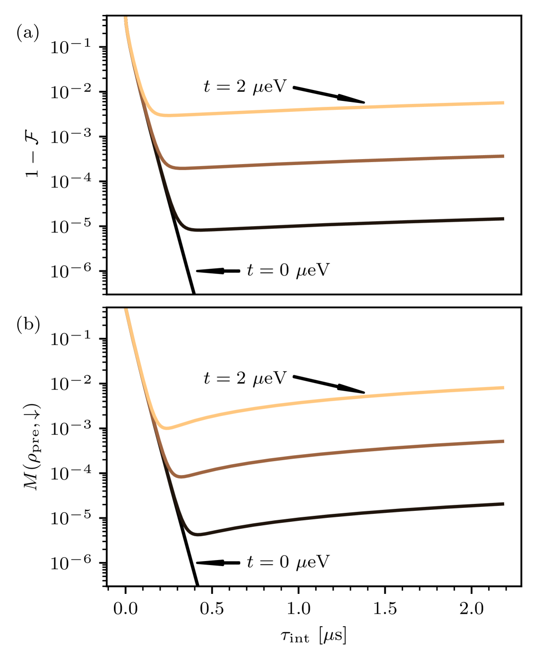
Infidelity, the metric we first consider, is expressed with the measurement operations as
| (2) |
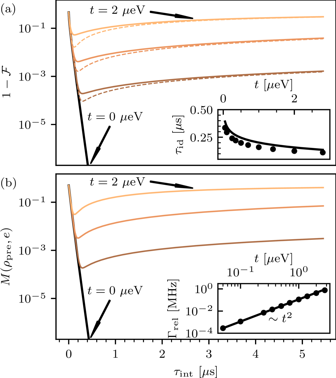
In Fig. 2a, we show the infidelity as a function of integration time . For short integration times, the infidelity decreases with increasing , since we gain more information about the initial state. For , the infidelity vanishes as . However, for , the infidelity increases after an ideal integration time . As we argue below, this increase is due to the back-action of the measurement that leads to qubit relaxation.
The time dependence of the infidelity in Fig. 2a is explained as follows. The pace of information gain upon readout is quantified by the measurement rate , i.e., the decay rate of the overlap between the two distributions of the transmission ratio corresponding to pre-measurement states and . This overlap has the form , through which is defined, where is the cumulative distribution function of the normal distribution. Upon calculating up to lowest (zeroth) order in (see SM S3), which is the relevant limit at the readout point, we find
| (3) |
This rate characterizes the decrease of the infidelity in Fig. 2a for short integration times.
A nonzero residual tunneling implies the non-commutativity relation . This, in turn, implies readout back-action in the form of qubit relaxation Goan et al. (2001); Boissonneault et al. (2009) characterized by the relaxation rate , which we express (see SM S4) as:
| (4) |
This rate quantifies the speed at which the unconditional post-measurement state approaches the completely mixed state. The inset of Fig. 2b shows that Eq. (4) (solid line) matches the relaxation rates obtained numerically (points) for the investigated parameter range. Note that Eq. (4) is not valid if the argument of the sine is close to , (see SM S4).
The second readout metric we consider is the mixedness of the post-measurement state. In a projective measurement of a qubit, the post-measurement state is pure. However, in our setup, the post-measurement state is mixed, unless in the special case and . The post-measurement state depends on the pre-measurement state and the measurement outcome . We express the mixedness of the post-measurement state with the measurement operations as
| (5) |
with the conditional post-measurement state . A nonzero mixedness indicates deviations from a projective measurement. In Fig. 2b, the mixedness for outcome is shown for the fully mixed pre-measurement state, as a function of integration time. The qualitative dependence of the mixedness on integration time is similar to that of the infidelity, and is well described by the measurement and relaxation rates.
These results confirm that a residual tunneling causes imperfect readout, thus it is critical to accurately control . Below, we argue that the same conclusion applies for Pauli-blockade-based spin qubit readout.
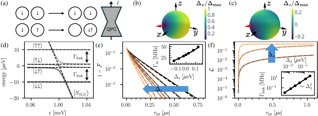
Spin qubit. Readout of spin qubits is often relies on Pauli blockade for spin-to-charge conversion and subsequent charge sensing Nurizzo et al. (2023); Blumoff et al. (2022); Harvey-Collard et al. (2018). Here, we generalize the QMQ model to describe such a readout. We focus on Pauli-blockade readout of a single-electron (Loss-DiVincenzo Loss and DiVincenzo (1998)) spin qubit. This requires a DQD with a target spin to be measured in, say, the right dot and a know reference spin in the left dot, see Fig. 3a. Readout is done in three steps: spin-to-charge conversion, charge sensing and charge-to-spin conversion. Without relaxation processes, this readout is non-destructive.
We model the two-electron DQD by the Hamiltonian of a two-site Hubbard model:
| (6) |
where , , , , is an electronic creation operator on dot with spin , and . Furthermore, is the Zeeman energy in dot due to a magnetic field , proportional to the -factor of dot , and is the Coulomb repulsion energy between two electrons occupying the same dot. At this point, spin-orbit interaction is included in Eq. (6) by considering different -factors in the two dots.
For later use, we introduce the six two-electron basis states , , etc, with denoting the state of the empty DQD. These states are eigenstates of at . The detuning dependence of the five lowest-energy states for is illustrated in Fig. 3d as the dashed lines. We focus on readout errors due to the back-action of the charge sensor. Therefore, we assume perfect state transfer during spin-to-charge and charge-to-spin conversion between the computational states at the operational point (left end of Fig. 3d) and the the computational states at the readout point (right end of Fig. 3d) according to, say, and .
The interaction between the DQD and the QPC is described by the term
| (7) |
which is a natural generalization of in Eq. (1). This captures that the transmission probability of the QPC is lower if there are two electrons in the right dot, instead of one.
We use this model to describe readout of the spin qubit in dot . The measurement operations and are computed analogously to those of the charge qubit readout as a function of model parameters.
Ideally, tunnel coupling is switched off at the readout position for the time window labeled by . However, in a given device, it might be impossible to set , which enhances readout errors, akin to the case of the charge qubit discussed above. A small but nonzero residual tunneling fulfilling and implies that is slightly hybridized with and ; the perturbed eigenstates are denoted by , , and . As a consequence, the interaction of the DQD with the QPC electrons leads to incoherent transitions between the state and the states and . The measurement benchmarks infidelity and mixedness show the same qualitative behavior as illustrated in Fig. 2 for the charge qubit. We discuss this back-action for the spin qubit in more detail in SM S6.
From now on, we assume that the tunnel coupling can be switched off (). In this case, another mechanism affecting readout is the spin-orbit mediated interaction between the DQD spins and the fluctuating electric field created by the QPC electrons Kato et al. (2003); Borhani et al. (2006); Crippa et al. (2018); Venitucci et al. (2018); Studenikin et al. (2019), often described as -tensor modulation. To account for this, we generalize the interaction Hamiltonian of Eq. (7) as
| (8) |
where describes the spin-charge coupling, i.e., change of the -tensor on dot caused by the electric field of the charges flowing through the QPC. Here, is a real matrix, and represents the spin vector on the right dot, e.g., . The joint Hamiltonian of the system and the meter is given by Eq. (6), Eq. (8) with , and in Eq. (1).
First, we discuss the special case when the modulation of the Zeeman field is perpendicular to the static Zeeman field, i.e. . In this case, it holds that , which leads to leakage from the computational state to the state , which is outside of the computational subspace (see SM S4). The leakage probability for a pre-measurement state of the computational subspace at the readout point is expressed as
| (9) |
where , and .
Of the two computational basis states, is not prone to readout-induced leakage, but is. Numerical results for leakage from are shown with solid lines in Fig. 3f. Longer integration times lead to increased leakage, saturating at ; increasing the coupling strength also increases leakage. Analytical derivations (SM S4) for this case show that leakage can be expressed as , with the leakage rate
| (10) |
This analytical result for the leakage is shown in Fig. 3f as dashed lines, matching well the numerical results. This leakage mechanism, although undesired as it corrupts the post-measurement state, does not affect the readout infidelity, as the sensor does not differentiate between and .
Second, we discuss the case when the modulation of the Zeeman field is parallel to the static Zeeman field, i.e. . Then, it holds that , hence, there is no relaxation or leakage, and the infidelity goes to zero as . This is shown numerically in Fig. 3e, as the solid lines. Fig. 3e also reveals that for a given integration time, infidelity decreases and hence readout improves as is increased. This improvement is due to the spin-charge coupling term of Eq. (8), which, in this special case, makes the QPC current dependent on and hence facilitates readout. This is explained by expressing in the two-dimensional computational subspace, resulting in , up to a global energy shift. Therefore, we substitute in Eq. (3), and we conclude that shows an approximately linear dependence on for . This is confirmed by the inset of Fig. 3e, where the above analytical approximation (solid) is compared to results (dots) obtained by fitting the function on the infidelity data in Fig. 3e.
The above results imply that leakage is eliminated in a magnetic field configuration where the static Zeeman field in dot is parallel to the local Zeeman field fluctuation caused the QPC. Interestingly, this can be achieved for any generic -tensor and matrix: the equation for the unknown is solved by the right eigenvectors of , and the latter matrix has either 1 or 3 real eigenvalue-eigenvector pairs, which describe physical magnetic-field directions Sen et al. (2023). In the case of 3 real eigenvectors, it is optimal to orient the magnetic field along that of the greatest eigenvalue, to maximize the measurement rate . The above consideration identifies a readout sweet spot in terms of the magnetic-field direction, akin to dephasing and relaxation sweet spots identified earlier Piot et al. (2022); Sen et al. (2023); Michal et al. (2023); Mauro et al. (2024); Bosco and Loss (2021); Bosco et al. (2021a); Malkoc et al. (2022). The red arrow in Figs. 3c,d show the readout sweet spot for a the -tensor and -tensor modulation from Crippa et al. (2018), for which there is a single real eigenvalue of . In a multi-qubit device, in-situ tuning of the -tensor parameters by gate voltages Crippa et al. (2018); Piot et al. (2022); Hendrickx et al. (2024); John et al. (2025); Rimbach-Russ et al. (2024); Bosco et al. (2021a, 2022, b); Saez-Mollejo et al. (2024); Carballido et al. (2024); Bassi et al. (2024) could be used to synchronize the readout sweet spots.
Conclusions. We have identified two sources of readout error for quantum-dot-based charge and spin qubits: residual tunneling and -tensor modulation. We have characterized the parameter dependence of these errors via a minimal model for the readout process, going beyond readout infidelity, describing mixedness of the post-measurement state and leakage, serving as key benchmark for the quantum protocols that recycle qubits after measuring them. Our results provide clear guidelines to optimize readout by full control of the tunnel coupling and exploiting magnetic readout sweet spots, and open the way to understand and minimize measurement errors for a variety of charge sensing techniques.
Acknowledgments. We thank Gy. Frank, B. Kolok, R. Németh, E. G. Kelly, P. Harvey-Collard for fruitful discussions. This work was supported by the Ministry of Culture and Innovation and the National Research, Development and Innovation Office within the Quantum Information National Laboratory of Hungary, Grant No. 2022-2.1.1-NL-2022-00004 (SD, GSz, AP); via the EKÖP_KDP-24-1-BME-2 funding scheme through Project Nr. 2024-2.1.2-EKÖP-KDP-2024-00005 (SD, AP); and by the European Union within the Horizon Europe research and innovation programme via the projects IGNITE (SD, AP), ONCHIPS (SD, AP), and QLSI2 (SD, SB, AP). This work was supported by the HUN-REN Hungarian Research Network through the Supported Research Groups Programme, HUN-REN-BME-BCE Quantum Technology Research Group (TKCS-2024/34). GSz was supported by the János Bolyai Research Scholarship of the Hungarian Academy of Science. BH, SB, and DL also acknowledge support from NCCR Spin (grant number 225153) and the NCCR Spin Mobility Grant. SB was sponsored in part by the Army Research Office, Award Number: W911NF-23-1-0110. The views and conclusions contained in this document are those of the authors and should not be interpreted as representing the official policies, either expressed or implied, of the Army Research Office or the U.S. Government. The U.S. Government is authorized to reproduce and distribute reprints for Government purposes notwithstanding any copyright notation herein.
References
- Loss and DiVincenzo (1998) D. Loss and D. P. DiVincenzo, Phys. Rev. A 57, 120 (1998).
- Hanson et al. (2007) R. Hanson, L. P. Kouwenhoven, J. R. Petta, S. Tarucha, and L. M. K. Vandersypen, Rev. Mod. Phys. 79, 1217 (2007).
- Zwanenburg et al. (2013) F. A. Zwanenburg, A. S. Dzurak, A. Morello, M. Y. Simmons, L. C. L. Hollenberg, G. Klimeck, S. Rogge, S. N. Coppersmith, and M. A. Eriksson, Rev. Mod. Phys. 85, 961 (2013).
- Eriksson et al. (2004) M. Eriksson, M. Friesen, S. Coppersmith, R. Joynt, L. Klein, K. Slinker, C. Tahan, P. Mooney, J. Chu, and S. Koester, Quantum Information Processing 3 (2004).
- Burkard et al. (2023) G. Burkard, T. D. Ladd, A. Pan, J. M. Nichol, and J. R. Petta, Rev. Mod. Phys. 95, 025003 (2023).
- Wang et al. (2024) C.-A. Wang, V. John, H. Tidjani, C. X. Yu, A. S. Ivlev, C. Déprez, F. van Riggelen-Doelman, B. D. Woods, N. W. Hendrickx, W. I. L. Lawrie, L. E. A. Stehouwer, S. D. Oosterhout, A. Sammak, M. Friesen, G. Scappucci, S. L. de Snoo, M. Rimbach-Russ, F. Borsoi, and M. Veldhorst, Science 385, 447 (2024).
- Zhang et al. (2025a) X. Zhang, E. Morozova, M. Rimbach-Russ, D. Jirovec, T.-K. Hsiao, P. C. Fariña, C.-A. Wang, S. D. Oosterhout, A. Sammak, G. Scappucci, M. Veldhorst, and L. M. K. Vandersypen, Nature Nanotechnology 20, 209 (2025a).
- Philips et al. (2022) S. G. J. Philips, M. T. Mądzik, S. V. Amitonov, S. L. de Snoo, M. Russ, N. Kalhor, C. Volk, W. I. L. Lawrie, D. Brousse, L. Tryputen, B. P. Wuetz, A. Sammak, M. Veldhorst, G. Scappucci, and L. M. K. Vandersypen, Nature 609, 919 (2022).
- Hendrickx et al. (2021) N. W. Hendrickx, W. I. L. Lawrie, M. Russ, F. van Riggelen, S. L. de Snoo, R. N. Schouten, A. Sammak, G. Scappucci, and M. Veldhorst, Nature 591, 580 (2021).
- Kloeffel and Loss (2013) C. Kloeffel and D. Loss, Annual Review of Condensed Matter Physics 4, 51 (2013).
- Vandersypen et al. (2017) L. M. K. Vandersypen, H. Bluhm, J. S. Clarke, A. S. Dzurak, R. Ishihara, A. Morello, D. J. Reilly, L. R. Schreiber, and M. Veldhorst, npj Quantum Information 3, 34 (2017).
- Scappucci et al. (2021) G. Scappucci, C. Kloeffel, F. A. Zwanenburg, D. Loss, M. Myronov, J.-J. Zhang, S. D. Franceschi, G. Katsaros, and M. Veldhorst, Nature Reviews Materials 6, 926 (2021).
- Stano and Loss (2022) P. Stano and D. Loss, Nature Reviews Physics 4, 672 (2022).
- Maurand et al. (2016) R. Maurand, X. Jehl, D. Kotekar-Patil, A. Corna, H. Bohuslavskyi, R. Laviéville, L. Hutin, S. Barraud, M. Vinet, M. Sanquer, and S. De Franceschi, Nature Communications 7, 13575 (2016).
- Xue et al. (2021) X. Xue, B. Patra, J. P. G. van Dijk, N. Samkharadze, S. Subramanian, A. Corna, B. Paquelet Wuetz, C. Jeon, F. Sheikh, E. Juarez-Hernandez, B. P. Esparza, H. Rampurawala, B. Carlton, S. Ravikumar, C. Nieva, S. Kim, H.-J. Lee, A. Sammak, G. Scappucci, M. Veldhorst, F. Sebastiano, M. Babaie, S. Pellerano, E. Charbon, and L. M. K. Vandersypen, Nature 593, 205 (2021).
- Jirovec et al. (2021) D. Jirovec, A. Hofmann, A. Ballabio, P. M. Mutter, G. Tavani, M. Botifoll, A. Crippa, J. Kukucka, O. Sagi, F. Martins, J. Saez-Mollejo, I. Prieto, M. Borovkov, J. Arbiol, D. Chrastina, G. Isella, and G. Katsaros, Nature Materials 20, 1106 (2021).
- Liles et al. (2024) S. D. Liles, D. J. Halverson, Z. Wang, A. Shamim, R. S. Eggli, I. K. Jin, J. Hillier, K. Kumar, I. Vorreiter, M. J. Rendell, J. Y. Huang, C. C. Escott, F. E. Hudson, W. H. Lim, D. Culcer, A. S. Dzurak, and A. R. Hamilton, Nature Communications 15, 7690 (2024).
- Camenzind et al. (2022) L. C. Camenzind, S. Geyer, A. Fuhrer, R. J. Warburton, D. M. Zumbühl, and A. V. Kuhlmann, Nature Electronics 5, 178 (2022).
- Zwerver et al. (2022) A. M. J. Zwerver, T. Krähenmann, T. F. Watson, L. Lampert, H. C. George, R. Pillarisetty, S. A. Bojarski, P. Amin, S. V. Amitonov, J. M. Boter, R. Caudillo, D. Correas-Serrano, J. P. Dehollain, G. Droulers, E. M. Henry, R. Kotlyar, M. Lodari, F. Lüthi, D. J. Michalak, B. K. Mueller, S. Neyens, J. Roberts, N. Samkharadze, G. Zheng, O. K. Zietz, G. Scappucci, M. Veldhorst, L. M. K. Vandersypen, and J. S. Clarke, Nature Electronics 5, 184 (2022).
- Neyens et al. (2024) S. Neyens, O. K. Zietz, T. F. Watson, F. Luthi, A. Nethwewala, H. C. George, E. Henry, M. Islam, A. J. Wagner, F. Borjans, E. J. Connors, J. Corrigan, M. J. Curry, D. Keith, R. Kotlyar, L. F. Lampert, M. T. Mądzik, K. Millard, F. A. Mohiyaddin, S. Pellerano, R. Pillarisetty, M. Ramsey, R. Savytskyy, S. Schaal, G. Zheng, J. Ziegler, N. C. Bishop, S. Bojarski, J. Roberts, and J. S. Clarke, Nature 629, 80 (2024).
- Geyer et al. (2024) S. Geyer, B. Hetényi, S. Bosco, L. C. Camenzind, R. S. Eggli, A. Fuhrer, D. Loss, R. J. Warburton, D. M. Zumbühl, and A. V. Kuhlmann, Nature Physics 20, 1152 (2024).
- Steinacker et al. (2024) P. Steinacker, N. D. Stuyck, W. H. Lim, T. Tanttu, M. Feng, A. Nickl, S. Serrano, M. Candido, J. D. Cifuentes, F. E. Hudson, K. W. Chan, S. Kubicek, J. Jussot, Y. Canvel, S. Beyne, Y. Shimura, R. Loo, C. Godfrin, B. Raes, S. Baudot, D. Wan, A. Laucht, C. H. Yang, A. Saraiva, C. C. Escott, K. D. Greve, and A. S. Dzurak, A 300 mm foundry silicon spin qubit unit cell exceeding 99% fidelity in all operations (2024), arXiv:2410.15590 [cond-mat.mes-hall] .
- Xue et al. (2022) X. Xue, M. Russ, N. Samkharadze, B. Undseth, A. Sammak, G. Scappucci, and L. M. K. Vandersypen, Nature 601, 343 (2022).
- Noiri et al. (2022) A. Noiri, K. Takeda, T. Nakajima, T. Kobayashi, A. Sammak, G. Scappucci, and S. Tarucha, Nature 601, 338 (2022).
- Mills et al. (2022) A. R. Mills, C. R. Guinn, M. J. Gullans, A. J. Sigillito, M. M. Feldman, E. Nielsen, and J. R. Petta, Science Advances 8, eabn5130 (2022).
- Takeda et al. (2024) K. Takeda, A. Noiri, T. Nakajima, L. C. Camenzind, T. Kobayashi, A. Sammak, G. Scappucci, and S. Tarucha, npj Quantum Information 10, 22 (2024).
- Harvey-Collard et al. (2018) P. Harvey-Collard, B. D’Anjou, M. Rudolph, N. T. Jacobson, J. Dominguez, G. A. Ten Eyck, J. R. Wendt, T. Pluym, M. P. Lilly, W. A. Coish, M. Pioro-Ladrière, and M. S. Carroll, Phys. Rev. X 8, 021046 (2018).
- Blumoff et al. (2022) J. Z. Blumoff, A. S. Pan, T. E. Keating, R. W. Andrews, D. W. Barnes, T. L. Brecht, E. T. Croke, L. E. Euliss, J. A. Fast, C. A. Jackson, A. M. Jones, J. Kerckhoff, R. K. Lanza, K. Raach, B. J. Thomas, R. Velunta, A. J. Weinstein, T. D. Ladd, K. Eng, M. G. Borselli, A. T. Hunter, and M. T. Rakher, PRX Quantum 3, 010352 (2022).
- Nurizzo et al. (2023) M. Nurizzo, B. Jadot, P.-A. Mortemousque, V. Thiney, E. Chanrion, D. Niegemann, M. Dartiailh, A. Ludwig, A. D. Wieck, C. Bäuerle, M. Urdampilleta, and T. Meunier, PRX Quantum 4, 010329 (2023).
- Vigneau et al. (2023) F. Vigneau, F. Fedele, A. Chatterjee, D. Reilly, F. Kuemmeth, M. F. Gonzalez-Zalba, E. Laird, and N. Ares, Applied Physics Reviews 10, 021305 (2023).
- Pereira et al. (2022) L. Pereira, J. J. García-Ripoll, and T. Ramos, Phys. Rev. Lett. 129, 010402 (2022).
- Pereira et al. (2023) L. Pereira, J. J. García-Ripoll, and T. Ramos, npj Quantum Information 9, 22 (2023).
- Rudinger et al. (2022) K. Rudinger, G. J. Ribeill, L. C. Govia, M. Ware, E. Nielsen, K. Young, T. A. Ohki, R. Blume-Kohout, and T. Proctor, Phys. Rev. Appl. 17, 014014 (2022).
- Zhang et al. (2025b) Z. Zhang, S. Chen, Y. Liu, and L. Jiang, PRX Quantum 6, 010310 (2025b).
- Hines and Proctor (2025) J. Hines and T. Proctor, Phys. Rev. Lett. 134, 020602 (2025).
- Hothem et al. (2024) D. Hothem, J. Hines, C. Baldwin, D. Gresh, R. Blume-Kohout, and T. Proctor, Measuring error rates of mid-circuit measurements (2024), arXiv:2410.16706 [quant-ph] .
- McLaren et al. (2025) D. McLaren, M. A. Graydon, A. A. Mahmoud, and J. J. Wallman, Benchmarking quantum instruments (2025), arXiv:2502.00179 [quant-ph] .
- Miao et al. (2023) K. C. Miao, M. McEwen, J. Atalaya, D. Kafri, L. P. Pryadko, A. Bengtsson, A. Opremcak, K. J. Satzinger, Z. Chen, P. V. Klimov, C. Quintana, R. Acharya, K. Anderson, M. Ansmann, F. Arute, K. Arya, A. Asfaw, J. C. Bardin, A. Bourassa, J. Bovaird, L. Brill, B. B. Buckley, D. A. Buell, T. Burger, B. Burkett, N. Bushnell, J. Campero, B. Chiaro, R. Collins, P. Conner, A. L. Crook, B. Curtin, D. M. Debroy, S. Demura, A. Dunsworth, C. Erickson, R. Fatemi, V. S. Ferreira, L. F. Burgos, E. Forati, A. G. Fowler, B. Foxen, G. Garcia, W. Giang, C. Gidney, M. Giustina, R. Gosula, A. Grajales Dau, J. A. Gross, M. C. Hamilton, S. D. Harrington, P. Heu, J. Hilton, M. R. Hoffmann, S. Hong, T. Huang, A. Huff, J. Iveland, E. Jeffrey, Z. Jiang, C. Jones, J. Kelly, S. Kim, F. Kostritsa, J. M. Kreikebaum, D. Landhuis, P. Laptev, L. Laws, K. Lee, B. J. Lester, A. T. Lill, W. Liu, A. Locharla, E. Lucero, S. Martin, A. Megrant, X. Mi, S. Montazeri, A. Morvan, O. Naaman, M. Neeley, C. Neill, A. Nersisyan, M. Newman, J. H. Ng, A. Nguyen, M. Nguyen, R. Potter, C. Rocque, P. Roushan, K. Sankaragomathi, H. F. Schurkus, C. Schuster, M. J. Shearn, A. Shorter, N. Shutty, V. Shvarts, J. Skruzny, W. C. Smith, G. Sterling, M. Szalay, D. Thor, A. Torres, T. White, B. W. K. Woo, Z. J. Yao, P. Yeh, J. Yoo, G. Young, A. Zalcman, N. Zhu, N. Zobrist, H. Neven, V. Smelyanskiy, A. Petukhov, A. N. Korotkov, D. Sank, and Y. Chen, Nature Physics 19, 1780 (2023).
- McEwen et al. (2021) M. McEwen, D. Kafri, Z. Chen, J. Atalaya, K. J. Satzinger, C. Quintana, P. V. Klimov, D. Sank, C. Gidney, A. G. Fowler, F. Arute, K. Arya, B. Buckley, B. Burkett, N. Bushnell, B. Chiaro, R. Collins, S. Demura, A. Dunsworth, C. Erickson, B. Foxen, M. Giustina, T. Huang, S. Hong, E. Jeffrey, S. Kim, K. Kechedzhi, F. Kostritsa, P. Laptev, A. Megrant, X. Mi, J. Mutus, O. Naaman, M. Neeley, C. Neill, M. Niu, A. Paler, N. Redd, P. Roushan, T. C. White, J. Yao, P. Yeh, A. Zalcman, Y. Chen, V. N. Smelyanskiy, J. M. Martinis, H. Neven, J. Kelly, A. N. Korotkov, A. G. Petukhov, and R. Barends, Nature Communications 12, 1761 (2021).
- Battistel et al. (2021) F. Battistel, B. Varbanov, and B. Terhal, PRX Quantum 2, 030314 (2021).
- Marques et al. (2023) J. F. Marques, H. Ali, B. M. Varbanov, M. Finkel, H. M. Veen, S. L. M. van der Meer, S. Valles-Sanclemente, N. Muthusubramanian, M. Beekman, N. Haider, B. M. Terhal, and L. DiCarlo, Phys. Rev. Lett. 130, 250602 (2023).
- Liepelt et al. (2024) M. Liepelt, T. Peduzzi, and J. R. Wootton, Journal of Physics A: Mathematical and Theoretical 57, 255302 (2024).
- Gehér et al. (2024) G. P. Gehér, M. Jastrzebski, E. T. Campbell, and O. Crawford, To reset, or not to reset – that is the question (2024), arXiv:2408.00758 [quant-ph] .
- Tornow et al. (2022) C. Tornow, N. Kanazawa, W. E. Shanks, and D. J. Egger, Phys. Rev. Appl. 17, 064061 (2022).
- Bäumer et al. (2024) E. Bäumer, V. Tripathi, D. S. Wang, P. Rall, E. H. Chen, S. Majumder, A. Seif, and Z. K. Minev, PRX Quantum 5, 030339 (2024).
- Fleury et al. (2024) A. Fleury, J. Brown, E. Lloyd, M. Hernandez, and I. H. Kim, Journal of Chemical Theory and Computation 20, 10807–10816 (2024).
- Stenger et al. (2025) J. P. T. Stenger, G. Bazargan, N. T. Bronn, and D. Gunlycke, Method for simulating open-system dynamics using mid-circuit measurements on a quantum computer (2025), arXiv:2504.15187 [quant-ph] .
- Bäumer et al. (2024) E. Bäumer, V. Tripathi, A. Seif, D. Lidar, and D. S. Wang, Quantum fourier transform using dynamic circuits (2024), arXiv:2403.09514 [quant-ph] .
- Cao and Eisert (2025) C. Cao and J. Eisert, Measurement-driven quantum advantages in shallow circuits (2025), arXiv:2505.04705 [quant-ph] .
- Ono et al. (2002) K. Ono, D. G. Austing, Y. Tokura, and S. Tarucha, Science 297, 1313 (2002).
- Petta et al. (2005) J. R. Petta, A. C. Johnson, J. M. Taylor, E. A. Laird, A. Yacoby, M. D. Lukin, C. M. Marcus, M. P. Hanson, and A. C. Gossard, Science 309, 2180 (2005).
- Koppens et al. (2006) F. H. L. Koppens, C. Buizert, K. J. Tielrooij, I. T. Vink, K. C. Nowack, T. Meunier, L. P. Kouwenhoven, and L. M. K. Vandersypen, Nature 442, 766 (2006).
- Haldar et al. (2025) S. Haldar, M. Munk, H. Havir, W. Khan, S. Lehmann, C. Thelander, K. A. Dick, P. Samuelsson, P. P. Potts, and V. F. Maisi, Phys. Rev. Lett. 134, 023601 (2025).
- Taubert et al. (2008) D. Taubert, M. Pioro-Ladrière, D. Schröer, D. Harbusch, A. S. Sachrajda, and S. Ludwig, Phys. Rev. Lett. 100, 176805 (2008).
- Ferguson et al. (2020) M. S. Ferguson, L. C. Camenzind, C. Müller, D. E. F. Biesinger, C. P. Scheller, B. Braunecker, D. M. Zumbühl, and O. Zilberberg, Quantum measurement induces a many-body transition (2020), arXiv:2010.04635 [cond-mat.mes-hall] .
- Young and Clerk (2010) C. E. Young and A. A. Clerk, Phys. Rev. Lett. 104, 186803 (2010).
- Elzerman et al. (2003) J. M. Elzerman, R. Hanson, J. S. Greidanus, L. H. Willems van Beveren, S. De Franceschi, L. M. K. Vandersypen, S. Tarucha, and L. P. Kouwenhoven, Phys. Rev. B 67, 161308 (2003).
- Elzerman et al. (2004) J. M. Elzerman, R. Hanson, L. H. Willems van Beveren, B. Witkamp, L. M. K. Vandersypen, and L. P. Kouwenhoven, Nature 430, 431 (2004).
- Gustavsson et al. (2006) S. Gustavsson, R. Leturcq, B. Simovič, R. Schleser, T. Ihn, P. Studerus, K. Ensslin, D. C. Driscoll, and A. C. Gossard, Phys. Rev. Lett. 96, 076605 (2006).
- Wiseman and Milburn (2009) H. M. Wiseman and G. J. Milburn, Quantum Measurement and Control (Cambridge University Press, 2009).
- Diosi (2007) L. Diosi, A Short Course in Quantum Information Theory: An Approach From Theoretical Physics, Lecture Notes in Physics (Springer Berlin Heidelberg, 2007).
- Goan et al. (2001) H.-S. Goan, G. J. Milburn, H. M. Wiseman, and H. Bi Sun, Phys. Rev. B 63, 125326 (2001).
- Goan and Milburn (2001) H.-S. Goan and G. J. Milburn, Phys. Rev. B 64, 235307 (2001).
- Petersson et al. (2010) K. D. Petersson, J. R. Petta, H. Lu, and A. C. Gossard, Phys. Rev. Lett. 105, 246804 (2010).
- Scarlino et al. (2022) P. Scarlino, J. H. Ungerer, D. J. van Woerkom, M. Mancini, P. Stano, C. Müller, A. J. Landig, J. V. Koski, C. Reichl, W. Wegscheider, T. Ihn, K. Ensslin, and A. Wallraff, Phys. Rev. X 12, 031004 (2022).
- Meinersen et al. (2024) C. V. Meinersen, S. Bosco, and M. Rimbach-Russ, Quantum geometric protocols for fast high-fidelity adiabatic state transfer (2024), arXiv:2409.03084 [quant-ph] .
- Hashim et al. (2024) A. Hashim, L. B. Nguyen, N. Goss, B. Marinelli, R. K. Naik, T. Chistolini, J. Hines, J. P. Marceaux, Y. Kim, P. Gokhale, T. Tomesh, S. Chen, L. Jiang, S. Ferracin, K. Rudinger, T. Proctor, K. C. Young, R. Blume-Kohout, and I. Siddiqi, A practical introduction to benchmarking and characterization of quantum computers (2024), arXiv:2408.12064 [quant-ph] .
- Pyke (2018) R. Pyke, Journal of the Royal Statistical Society: Series B (Methodological) 27, 395 (2018).
- Boissonneault et al. (2009) M. Boissonneault, J. M. Gambetta, and A. Blais, Phys. Rev. A 79, 013819 (2009).
- Crippa et al. (2018) A. Crippa, R. Maurand, L. Bourdet, D. Kotekar-Patil, A. Amisse, X. Jehl, M. Sanquer, R. Laviéville, H. Bohuslavskyi, L. Hutin, S. Barraud, M. Vinet, Y.-M. Niquet, and S. De Franceschi, Phys. Rev. Lett. 120, 137702 (2018).
- Kato et al. (2003) Y. Kato, R. C. Myers, D. C. Driscoll, A. C. Gossard, J. Levy, and D. D. Awschalom, Science 299, 1201 (2003).
- Borhani et al. (2006) M. Borhani, V. N. Golovach, and D. Loss, Phys. Rev. B 73, 155311 (2006).
- Venitucci et al. (2018) B. Venitucci, L. Bourdet, D. Pouzada, and Y.-M. Niquet, Phys. Rev. B 98, 155319 (2018).
- Studenikin et al. (2019) S. Studenikin, M. Korkusinski, M. Takahashi, J. Ducatel, A. Padawer-Blatt, A. Bogan, D. G. Austing, L. Gaudreau, P. Zawadzki, A. Sachrajda, Y. Hirayama, L. Tracy, J. Reno, and T. Hargett, Communications Physics 2, 159 (2019).
- Sen et al. (2023) A. Sen, G. Frank, B. Kolok, J. Danon, and A. Pályi, Phys. Rev. B 108, 245406 (2023).
- Piot et al. (2022) N. Piot, B. Brun, V. Schmitt, S. Zihlmann, V. P. Michal, A. Apra, J. C. Abadillo-Uriel, X. Jehl, B. Bertrand, H. Niebojewski, L. Hutin, M. Vinet, M. Urdampilleta, T. Meunier, Y.-M. Niquet, R. Maurand, and S. D. Franceschi, Nature Nanotechnology 17, 1072 (2022).
- Michal et al. (2023) V. P. Michal, J. C. Abadillo-Uriel, S. Zihlmann, R. Maurand, Y.-M. Niquet, and M. Filippone, Phys. Rev. B 107, L041303 (2023).
- Mauro et al. (2024) L. Mauro, E. A. Rodríguez-Mena, M. Bassi, V. Schmitt, and Y.-M. Niquet, Phys. Rev. B 109, 155406 (2024).
- Bosco and Loss (2021) S. Bosco and D. Loss, Phys. Rev. Lett. 127, 190501 (2021).
- Bosco et al. (2021a) S. Bosco, B. Hetényi, and D. Loss, PRX Quantum 2, 010348 (2021a).
- Malkoc et al. (2022) O. Malkoc, P. Stano, and D. Loss, Phys. Rev. Lett. 129, 247701 (2022).
- Hendrickx et al. (2024) N. W. Hendrickx, L. Massai, M. Mergenthaler, F. J. Schupp, S. Paredes, S. W. Bedell, G. Salis, and A. Fuhrer, Nature Materials 23, 920 (2024).
- John et al. (2025) V. John, C. X. Yu, B. van Straaten, E. A. Rodríguez-Mena, M. Rodríguez, S. Oosterhout, L. E. A. Stehouwer, G. Scappucci, S. Bosco, M. Rimbach-Russ, Y.-M. Niquet, F. Borsoi, and M. Veldhorst, A two-dimensional 10-qubit array in germanium with robust and localised qubit control (2025), arXiv:2412.16044 [cond-mat.mes-hall] .
- Rimbach-Russ et al. (2024) M. Rimbach-Russ, V. John, B. van Straaten, and S. Bosco, A spinless spin qubit (2024), arXiv:2412.13658 [cond-mat.mes-hall] .
- Bosco et al. (2022) S. Bosco, P. Scarlino, J. Klinovaja, and D. Loss, Phys. Rev. Lett. 129, 066801 (2022).
- Bosco et al. (2021b) S. Bosco, M. Benito, C. Adelsberger, and D. Loss, Phys. Rev. B 104, 115425 (2021b).
- Saez-Mollejo et al. (2024) J. Saez-Mollejo, D. Jirovec, Y. Schell, J. Kukucka, S. Calcaterra, D. Chrastina, G. Isella, M. Rimbach-Russ, S. Bosco, and G. Katsaros, Exchange anisotropies in microwave-driven singlet-triplet qubits (2024), arXiv:2408.03224 [cond-mat.mes-hall] .
- Carballido et al. (2024) M. J. Carballido, S. Svab, R. S. Eggli, T. Patlatiuk, P. C. Kwon, J. Schuff, R. M. Kaiser, L. C. Camenzind, A. Li, N. Ares, E. P. A. M. Bakkers, S. Bosco, J. C. Egues, D. Loss, and D. M. Zumbühl, Compromise-free scaling of qubit speed and coherence (2024), arXiv:2402.07313 [cond-mat.mes-hall] .
- Bassi et al. (2024) M. Bassi, E.-A. Rodrıguez-Mena, B. Brun, S. Zihlmann, T. Nguyen, V. Champain, J. C. Abadillo-Uriel, B. Bertrand, H. Niebojewski, R. Maurand, Y.-M. Niquet, X. Jehl, S. D. Franceschi, and V. Schmitt, Optimal operation of hole spin qubits (2024), arXiv:2412.13069 .
Supplementary Material to
‘Readout sweet spots for spin qubits with strong spin-orbit interaction’
Domonkos Svastits1,2, Bence Hetényi3, Gábor Széchenyi4, James
Wotton3,5, Daniel Loss6, Stefano Bosco7, and András Pályi1,8
1Budapest University of Technology and Economics, Műegyetem rkp. 3., H-1111 Budapest, Hungary
2Qutility @ Faulhorn Labs, Budapest, Hungary
3BM Research Europe – Zurich, Säumerstrasse 4, 8803 Rüschlikon, Switzerland
4ELTE Eötvös Loránd University, Institute of Physics, H-1117 Budapest, Hungary
5Moth Quantum AG, Schorenweg 44B, 4144, Switzerland
6Department of Physics, University of Basel, Klingelbergstrasse 82, CH-4056 Basel, Switzerland
7QuTech and Kavli Institute of Nanoscience, Delft University of Technology, Delft, The Netherlands
8HUN-REN-BME-BCE Quantum Technology Research Group, Műegyetem rkp. 3., H-1111 Budapest, Hungary
(Dated: June 5, 2025)
S1 Details of describing QPC-based charge-sensing with the QMQ model
S1.1 Measurement operators of a single indirect measurement
Consider charge-qubit readout modeled with the Qubit Measures Qubit (QMQ) model, as described in the main text. Our model describes the readout process as a sequence of indirect measurements. The conditional post-measurement states of the qubit after a single indirect measurement are
| (S1a) | |||
| (S1b) | |||
given that the measurement of the meter resulted in a projection into the meter-state and respectively. Here, denotes unitary time evolution according to the Hamiltonian in Eq. (1) for the charge qubit; and the corresponding total Hamiltonian for the spin qubit. Furthermore, denotes tracing out the meter.
Simplifying Eq. (S1), we obtain
| (S2) |
Here, we defined the measurement operations and as well as the measurement operators Wiseman and Milburn (2009)
| (S3a) | |||
| (S3b) | |||
where the index labels the states of the qubit. The measurement operator () corresponds to finding the QPC-electron in the bottom (top) quantum dot.
To illustrate the measurement operators, we calculate their matrices for the charge qubit with in the computational basis :
| (S4a) | ||||
| (S4b) | ||||
| (S4c) | ||||
| (S4d) | ||||
| (S4e) | ||||
| (S4f) | ||||
In this work, we tune the parameters of the QMQ model in such a way that the probability () of transmission from the bottom dot to the top dot is slightly more (less) than 0.5, given that the data qubit electron is in the left (right) dot. Therefore, in the case above, a consequence of the formulas is that as follows: if a single indirect measurement it is easy to understand the effect of a single indirect measurement. For example, if we measure 0, the amplitude of being in the left dot decreases relative to the amplitude of being in the right dot. Recall that for , we have and .
It is often useful in both analytical (see SM S3 and S4) and numerical (see SM S1.5) calculations to use the transfer matrix representation of the measurement operation . The transfer matrix acts on the vectorized form of the density matrix Hashim et al. (2024) and it can be expressed using the matrix representation of the measurement operators as
| (S5) |
Equivalently, the transfer matrix elements can be expressed as . Here we introduced the notation , where is the dimension of the Hilbert space of the data qubit system. For the charge qubit , therefore the possible indices are 0, 1, 2 and 3. Note that the transfer matrices depend on the basis in which the measurement operators and density matrices are written. Throughout this work, we use the energy eigenbasis .
S1.2 Series of indirect measurements
As long as the interaction of the qubit and the meter is weak, many indirect measurements are needed to be able to distinguish the computational states and . The outcome of a series of indirect measurements is a bitstring of length . The corresponding measurement operator is
| (S6) |
To provide a full description of the measurement, one needs to evaluate the measurement operators corresponding to all possible bitstrings. The calculation and storage of the corresponding measurement operators is inefficient.
Although calculating all the measurement operators is in practice impossible for large , interesting quantities can still be calculated. In experiments, the initial state of the qubit is usually inferred based on the average current Haldar et al. (2025); Harvey-Collard et al. (2018); Blumoff et al. (2022); Nurizzo et al. (2023), i.e. the total number of transmitted electrons , which contains less information then the time dependence of the current, which is represented by . For our purposes, it is more convenient to use the transmission ratio instead of as the outcome of the measurement. The number of transmitted electrons and the transmission ratio both can take different values. The corresponding measurement operations are
| (S7) |
Note, that if and commute, the map takes pure states to pure states, i.e. the measurement is efficient Wiseman and Milburn (2009). In this case, no information is lost if only the transmission ratio is stored instead of the bitstring . We show in SM S1.5 how the measurement operations are efficiently computable numerically.
S1.3 Inference rule
The outcome of the readout is a time dependent current, which is represented as a bitstring in our model. Our aim is to infer the initial state based on the time dependent current. Therefore, we need an inference rule that assigns a single bit to . A possible approach would be to use the maximum likelihood inference rule based on all the available information in the model. This would require calculating the probabilities and of measuring given that the initial state was and respectively. Then, we would infer that the initial state was if ; otherwise we would infer . However, calculating and for all possible different bitstrings is inefficient.
Instead, we use the maximum likelihood inference rule, based on only the transmission ratio . This is motivated by experiments, where the average current is used to make this inference. To determine this inference rule, we need to calculate which initial state results in a higher probability of obtaining the transmission ratio , i.e., whether or is bigger. These probabilities are straightforward to calculate:
| (S8a) | |||
| (S8b) | |||
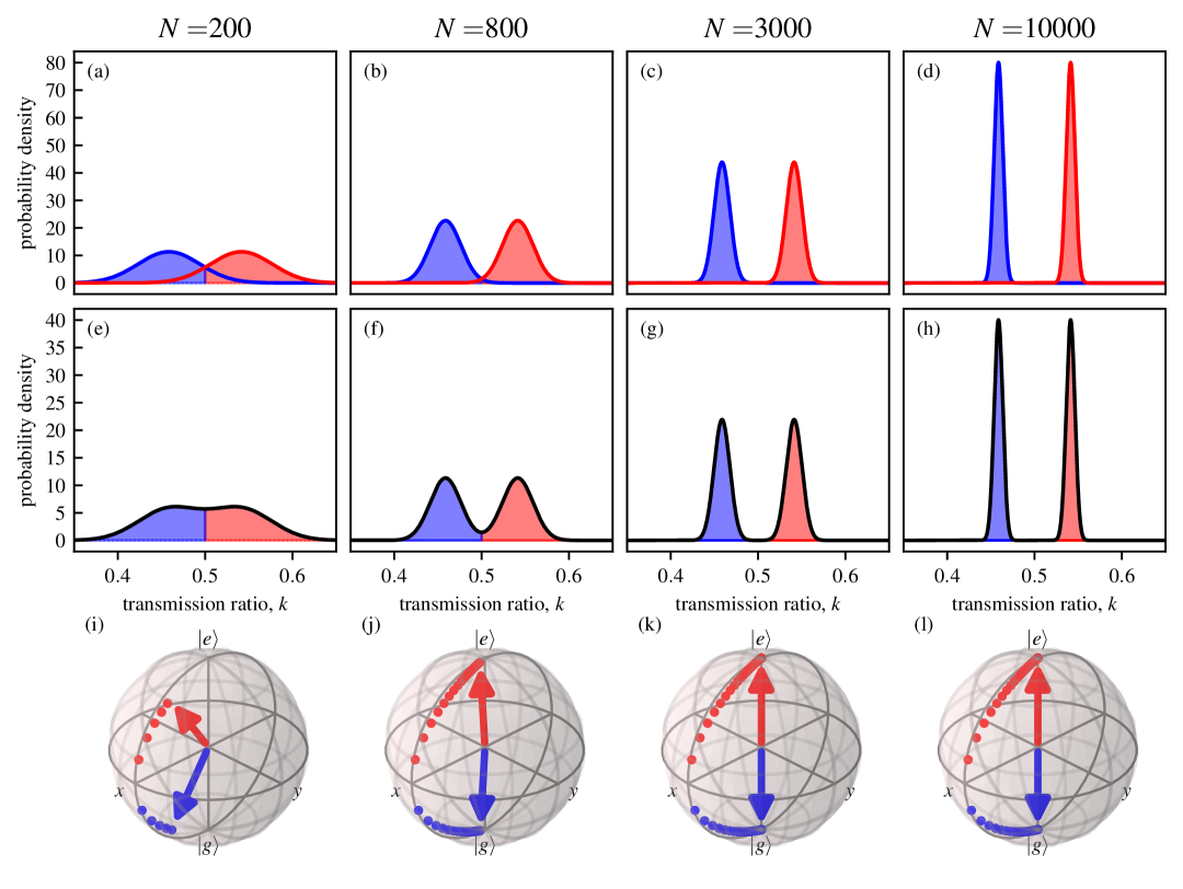
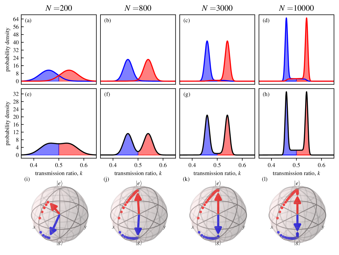
The resulting inference rule is the following: there is a critical transmission ratio , above (below) which we infer (). The probability mass functions and are efficiently calculable, therefore, so is the critical transmission ratio . In Figs. S1a-d and S2a-d, the probabilities and are plotted for different to illustrate the inference rule. The areas under the curves are colored red (blue) above (below) . Fig. S1 corresponds to the case of zero tunneling in the charge qubit (), and Fig. S2 corresponds to nonzero tunneling ().
In the case, the critical transmission ratio is easily determined analytically. Due to fixing as in Eq. (S12), we have and ; and and are defined in Eq. (S4). Then, by substituting Eqs. (S4) and (S7) into Eq. (S8), we obtain .
Furthermore, observe that in the case, (see Eq. (S4)), meaning that we discard no information by making the inference based on only the transmission ratio, as we have already discussed briefly below Eq. (S7). If , the timing of the transmission events does contain additional information, which is thrown away by this inference rule. It is an interesting open question how this additional information can be used to improve the inference of the initial data qubit state.
S1.4 Post-measurement state
Here we show how the post-measurement states corresponding to the inferred value are calculated. As detailed in the previous section, we use maximum likelihood inference based on the transmission ratio (see SM S1.3). This results in the following simple rule: we infer () if (). Therefore, the measurement operations belonging to the final outcome and are
| (S9a) | ||||
| (S9b) | ||||
These measurement operations give the post-measurement state given that we inferred or for the initial state. They can be calculated from the measurement operations using additions.
We plot the transmission ratio distributions and the post-measurement states for the initial state in Fig. S1e-l for zero residual tunneling and in S2e-l for finite residual tunneling. The post-measurement states move towards the two corresponding computational basis states at a time scale . For nonzero residual tunneling, relaxation of the qubit state also happens. This is apparent in Fig. S2i-l; for the parameter set used there, the relaxation time scale is much longer than .
S1.5 Efficient numerical simulation
Here, we show how the measurement operations in Eq. (S7) are computed efficiently. A brute-force approach would require calculating all measurement operators using Eq. (S6), and performing the summation in Eq. (S7). The computational costs of this approach scale exponentially with , making it impossible to carry out for large .
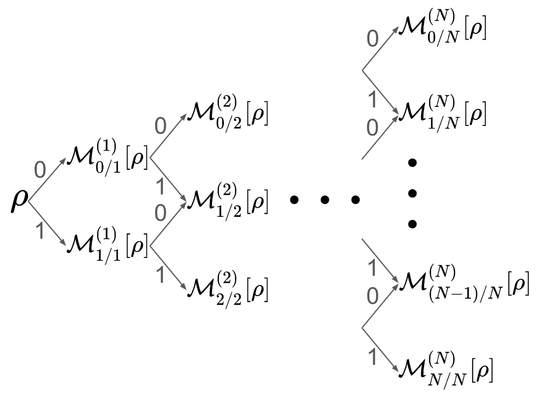
We instead calculate the measurement operations directly, using iteration in the number of indirect measurements. The iteration step is
| (S10) |
The iteration is illustrated in Fig. S3. In the th step of the iteration, can take different values, so we need to compute measurement operations. Let us call the computation of one measurement operation an elementary computation. Then the total number of elementary computations up to weak measurements is
| (S11) |
Note that the elementary computations of a single round can be parallelized.
In our numerical calculations, we represented the measurement operations as transfer matrices and performed the iteration in terms of these.
S2 Relating model parameters to experimental parameters
In our numerical calculations, we use experimentally constrained parameter values for calculating the measurement operations , ; and measurement benchmarks. To do this, we need to match the experimental parameters and the parameters of our model.
We fix the timestep between meter measurements as
| (S12) |
which corresponds to 0.5 transmission probability if the data qubit state is an equal superposition or mixture of the states and . This choice is motivated by experiments, since the conductance of a QPC is most sensitive to changes of charge configuration at the point, where its conductance is , i.e. half the conductance quantum Vigneau et al. (2023). In the QPC, there is only one open conductance channel, thus a conductance of means that any time an electron approaches the QPC, it tunnels through with probability . For the spin qubit, in the presence of a finite term, the same consideration leads to
| (S13) |
With this choice, the transmission probability is 0.5 if the qubit state is the equal superposition or mixture of the two computational states and .
Next, we calculate the current flowing through the QPC predicted by our model. The average current is
| (S14) |
where is the elementary charge. The difference between the currents corresponding to the states and is
| (S15) |
At the second equation mark, we expanded the sine functions up to first order around , using Eq. (S13) and the relation . Eqs. (S14) and (S15) connect the experimentally measurable currents and the model parameters.
The above relations lead us to the following experimentally realistic parameter set for the charge qubit Haldar et al. (2025):
| (S16a) | ||||
| (S16b) | ||||
| (S16c) | ||||
| (S16d) | ||||
For the spin qubit, we use the same values for the parameters and of the QPC. For parameters of the spin-Hamiltonian in Eq. (6), we used the parameter set
| (S17a) | ||||
| (S17b) | ||||
| (S17c) | ||||
| (S17d) | ||||
| (S17e) | ||||
which is experimentally realistic for electrons in AlGaAs/GaAs and Si/SiGe heterostructures Nurizzo et al. (2023); Blumoff et al. (2022); Harvey-Collard et al. (2018).
The integration time in experiments is around . In our model, current sensing is assumed to be perfect, consequently, according to our model, a measurement time much shorter than the above is sufficient to distinguish between the computational basis states of the data qubit. It is possible to incorporate imperfect current sensing into the model, by using inefficient Wiseman and Milburn (2009) meter measurements, however, we leave this generalization for later work.
S3 Dephasing and measurement rates
Here, we determine the dephasing and measurement rates for the case of zero tunneling amplitude. For finite, but small tunneling amplitude , the derived rates are the zeroth order approximations in of the actual rates. Here, we do the derivation for the charge qubit, but an analogous derivation works for the spin qubit as well.
The Hamiltonian of the charge qubit with zero tunneling amplitude is , which commutes with . Consequently, the measurement operators also commute:
| (S18) |
The matrix of these measurement operators in the computational basis is written in Eq. (S4), from which we get the transfer matrices using Eq. (S5):
| (S19a) | ||||
| (S19b) | ||||
Due to Eq. (S18), we have , which is also apparent from Eq. (S19). Therefore, the transfer matrix representing is
| (S20) |
This can than be written in the form
| (S21) |
where is the probability mass function of the binomial distribution.
The binomial distribution can be approximated by the a normal distribution for . Using this approximation and Eq. (S19), we get
| (S22a) | ||||
| (S22b) | ||||
where
| (S23a) | ||||
| (S23b) | ||||
Here, denotes the cumulative distribution function of the normal distribution. The matrix element () gives the probability of inferring () for the initial state (); and give how the off-diagonal density matrix elements evolve.
We now define the measurement and dephasing rates using Eqs. (S23a) and (S23b) respectively. The measurement rate characterizes the speed at which the two current distributions corresponding to the initial states and become distinguishable. We define it through
| (S24) |
The value of the measurement rate is obtained by comparing this definition with Eq. (S23a):
| (S25) |
At the second equation mark in Eq. (S25) we expanded up to second order in . For the spin qubit, the same calculation yields
| (S26a) | ||||
| (S26b) | ||||
where is the analogous quantity to for the spin qubit, i.e it is the difference of the transition probabilities for the states and . For this is exactly the same as the measurement rate for the charge qubit Eq. (S25).
The dephasing rate characterizes the speed at which the magnitude of the off-diagonal matrix elements decrease with time in the unconditional time evolution, i.e. it is defined through
| (S27) |
Its value is obtained by comparing this definition with Eq. (S23b):
| (S28) |
Similarly to the measurement rate, we expanded the dephasing rate up to second order in . We find, that up to this order, the two rates are the same for the charge qubit. For the spin qubit, an analogous calculation shows that for , the off-diagonal density matrix elements between the two computational states decay as
| (S29) |
with
| (S30) |
The time evolution of off-diagonal matrix elements connecting states outside of the computational subspace can be calculated analogously.
Our results show that the decrease of the off-diagonal density matrix elements and the separation of the two current distributions happen at the same time scale. Note that this approximate equality of the two rates holds only because we assume current sensing to be perfect in our model. Noisy current sensing does not change the dephasing rate, since it is defined through the unconditional time evolution. However, it decreases the measurement rate, i.e., increases the time needed to distinguish between the two computational states. Therefore, in practice, the dephasing rate sets an upper bound for the measurement rate.
S4 Relaxation rate
Here, we derive the relaxation rate Eq. (4) for the charge qubit. An analogous derivation results in the leakage rate Eq. (10) for the spin qubit. In the derivation, we use perturbation theory to determine the transfer matrix describing the unconditional time evolution of one timestep. In the charge qubit case, the transfer matrix is a matrix, which has an eigenvalue that is 1. Its second closest eigenvalue to 1 in terms of absolute value determines the speed at which the initial state approaches the steady state, therefore, it is related to the relaxation rate as . In the calculation, we determine the eigenvalue and from it the relaxation rate up to leading order in , and .
The derivation uses first order time dependent perturbation theory. The unperturbed Hamiltonian is , while the perturbation is the interaction Hamiltonian (see Eq. (1)). The first step is to determine the eigenvectors of and rewrite the interaction Hamiltonian in the eigenbasis of . Eigenvectors of can be written in the form , where is an eigenvector of and is an eigenvector of . Changing from the basis to the basis is achieved by the unitary matrix
| (S31a) | ||||
| (S31b) | ||||
| (S31c) | ||||
The interaction Hamiltonian in the eigenbasis of is given by
| (S32) |
Here, denotes the matrix of in the basis . The diagonal matrix elements of are the first-order energy corrections.
Now we show how the time evolution operator of the total system is calculated up to first order in using time dependent perturbation theory. The state is expanded in the eigenbasis of :
| (S33) |
Here is an eigenenergy of ; and and are eigenenergies of the and respectively. At the second equation mark, we split the expansion coefficients into zeroth and first order terms and . According to first order time dependent perturbation theory, we have
| (S34a) | ||||
| (S34b) | ||||
We used the notations and At the second equation mark, we used that the interaction Hamiltonian has the form . For the charge qubit, is the first factor of the tensor product in Eq. (S32). Therefore, we can write .
The time evolution operator is related to the expansion coefficients as follows:
| (S35) |
Therefore, up to first order, using Eq. (S34b) we get
| (S36) |
Using Eqs. (S36), (S3b), we get the matrix form of the measurement operators up to in the unperturbed basis:
| (S37a) | ||||
| (S37b) | ||||
By substituting the energy values of the charge qubit into Eq. (S37), we get
| (S38a) | |||
| (S38b) | |||
Note that these expressions depend on through and .
The transfer matrix describing the unconditional time evolution is given by
| (S39) |
Using Eq. (S37), we get
| (S40a) | ||||
| (S40b) | ||||
Recall that we use the notation . We got this result form first order time dependent perturbation theory, so the result is accurate to first order in . However, some matrix elements are accurate to second order. We have , therefore, if the matrix elements and do not contain zeroth order terms, the resulting matrix element of the transfer matrix is accurate to second order.
For the charge qubit, we get
| (S41) |
At the final equation mark, we rewrote to leading order in . This is a relevant limit, since experimentally usually holds during readout. The term in the matrix element is not obtained directly from the first order calculation, however, , since represents a trace preserving map. Using this relation, we can calculate up to , since we know up to .
We aim to diagonalize the transfer matrix to extract the relaxation rate from it. It is diagonal up to , but the 0th and 3rd diagonal elements are the same, therefore, the offdiagonal matrix elements and give contributions to the eigenvalues. For the relaxation rate, the relevant eigenmode of is and the corresponding eigenvalue is . Therefore, we get
| (S42) |
where we defined the relaxation rate
| (S43) |
This expression is true up to second order in both and .
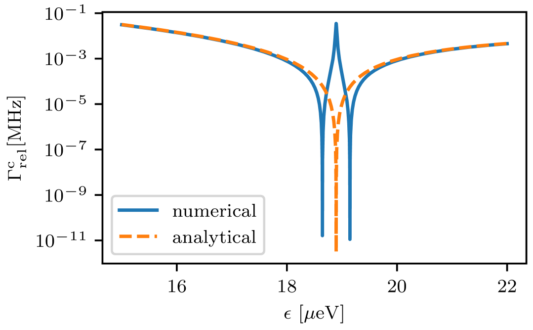
It is important to note that our expression is only valid if , since otherwise other offdiagonal elements of can give relevant contributions to the eigenvalues as well. Therefore, the expression should not be used, if , . This is confirmed by Fig. S4, where both analytically and numerically calculated values of the relaxation rate are shown. For the experimentally relevant parameter set that we used in our numerical calculations, the analytical results match the numerical data well as shown by the inset of Fig. 2(b).
For the spin qubit, in the presence of QPC-induced Zeeman field modulation described by Eq. (8), the same calculation shows that transitions between the states and ; and the states and are possible, leading to
| (S44a) | |||
| (S44b) | |||
The appearing rate is
| (S45) |
This rate characterizes leakage from the computational state to the state , which is not in the computational subspace during readout. Similarly to the charge qubit, this result is not valid if , . For the numerically investigated parameter values, the analytical formula gives a good estimate of the relaxation rate as shown by the inset of Fig. 3g.
S5 Analytical formula for readout fidelity and ideal integration time
Here, we derive an estimate for the fidelity that works well for both very short and long times. We obtain an order of magnitude estimate for the ideal integration time by finding the minimum of this infidelity function.
The estimate of the infidelity is
| (S46) |
where is the modified Bessel function of the first kind and is the cdf of the normal distribution. This analytical estimate of the fidelity is plotted in Fig. 2(a) together with the numerical results. We now discuss the considerations that lead to this estimate. The magnitude of the infidelity is determined by different features for short and long times. For very short times, for which relaxation is negligible, the current distributions corresponding to the two computational states are well approximated by Gaussians as shown by Fig. S2a,b. The infidelity is then due to the overlap of these Gaussians, which gives the contribution .
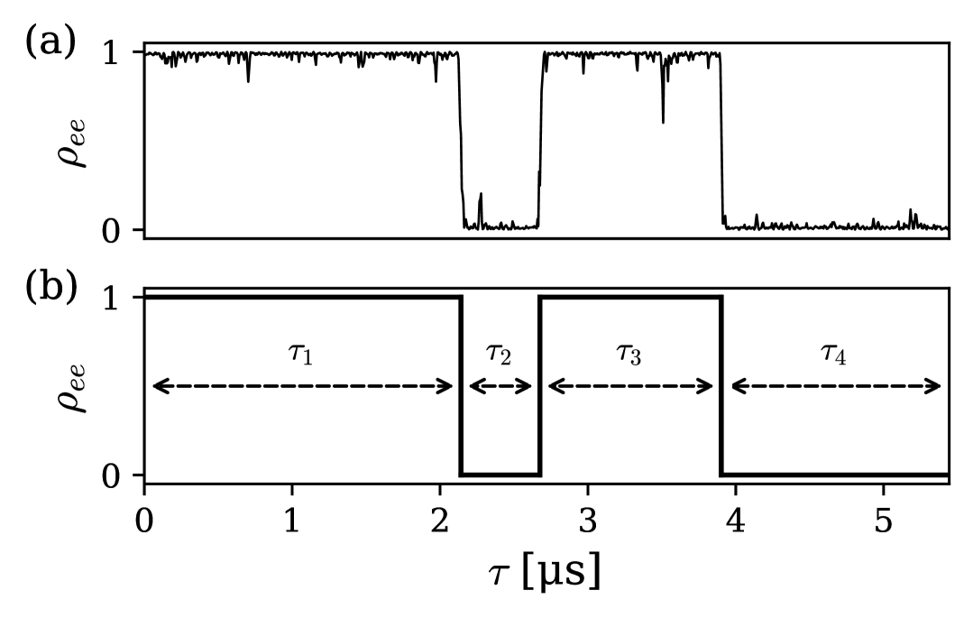
On the other hand, for long times the infidelity is mostly due to relaxation. Our estimate of this component of the infidelity is based on the observation that the qubit spends most of the time close to one of the computational basis states (see Fig S5). The expectation value of the current is () when the qubit is in state (). The time average of the current for a given trajectory is then well approximated by
| (S47) |
for long time , where and are the times spent in the excited and ground states respectively. The outcome is inferred if . Therefore, when starting from the initial state , an inference error is made if , which happens with probability . Similarly, for the initial state , an inference error is made if , which happens with probability . The rate of jumps from to is the same as the rate of jumps from to , therefore, the probabilities and are the same. For long times this probability gives the infidelity (see Eq. (2)). Therefore, the second error term in the infidelity estimate Eq. (S46) is .
Now we calculate the probability . To do this, we assume that the state is in exactly one of the computational basis states during the whole measurement and jumps between the two states are instantaneous and independent, as shown in Fig. S5b. The rate of jumps from one state to the other is (see Eq. (4)). Therefore, the problem is described by a symmetric random telegraph process. The jumps of a symmetric random telegraph process occur according to a Poisson process. We denote the waiting times between jumps as , , …, , … (see Fig. S5b).
Now we assume that exactly jumps occur during the integration time , which split the integration time into waiting times. Then the conditional probability of an inference error given that jumps occurred is
| (S48) |
The waiting times are described by the multivariate random variable .
The probability density function of is symmetric under exchanging the different waiting times, i.e, Pyke (2018). Therefore, the probability is the same as the probability that the sum of the first waiting times is less then , i.e. the probability that at least jumps occur in the time interval . The jump times are uniformly distributed in the interval and are independent. Therefore, we get
| (S49) |
This is the probability of an inference error given that jumps occur.
The probability distribution of the number of jumps is a Poisson distribution with parameter . Therefore, the probability of an inference error due to relaxation is given by
| (S50) |
where is the modified Bessel function of the first kind. This probability is the second term in the estimate of the infidelity Eq. (S46).
Now we derive an order of magnitude estimate for the ideal integration time by finding the minimum of the infidelity estimate. For and , we expect that Eq. (S46) provides a good approximation on the readout infidelity, since in each of these regions only one of the error mechanisms is significant. This suggests that the minimum of the infidelity estimate in Eq. (S46) provides a good order-of-magnitude estimate of the ideal integration time.
The derivative of Eq. (S46) is zero at , which leads to
| (S51) |
where . For high fidelity measurements, we have . We solve Eq. (S51) using this assumption, which leads to
| (S52) |
To get an order of magnitude estimate of , we can neglect the second term, since :
| (S53) |
The inset of Fig. 2a shows that this gives a good estimate of the numerically calculated values of the ideal integration time. Note that the ideal integration time scales logarithmically with the residual tunneling amplitude .
S6 Back-action due to residual tunneling for spin qubit
We have shown for a charge qubit that a nonzero residual tunneling during charge sensing leads to relaxation due to . The analogous relation is true for the spin qubit in the presence of a nonzero residual tunneling. Therefore, readout induces incoherent transitions between the energy eigenstates of the spin qubit.
The rates of these transitions can be calculated in the way as for the charge qubit (see SM S4). This calculation is performed in the eigenbasis of the spin qubit, therefore, the interaction Hamiltonian in Eq. (7) needs to be rewritten in the eigenbasis of , which is . We tilded the states to indicate that due to the finite tunneling amplitude, the energy eigenstates are not exactly the eigenstates of the spin operators.
Up to first order in , we obtain
| (S54a) | ||||
| (S54b) | ||||
| (S54c) | ||||
where .
An analogous derivation to the one in SM S4 then gives the transition rates
| (S55a) | |||
| (S55b) | |||
which are accurate to second order in . These rates are analogous to the transition rate of the charge qubit: incoherent transitions are induced between the eigenstates of the data qubit Hamiltonian that are connected by finite matrix elements of the interaction Hamiltonian.
The measurement benchmarks infidelity and mixedness as a function of integration time show the same qualitative behavior as for the charge qubit as shown by the numerical results in Fig. S6. The same analytical estimate for the fidelity is not possible for the spin qubit as for the charge qubit (see SM S5), since transitions happen between three states, not only two.
S7 Comparison with the stochastic master equation
Here, we compare the QMQ model with a previously used description of QPC-based readout that uses a stochastic Schrödinger equation (SSE) or a stochastic master equation (SME). We make the comparison using the example of charge qubit readout, however, our statements straightforwardly generalize to spin qubit readout. We show that the SSE description and the QMQ model give the same qualitative predictions. We also make quantitative comparison by comparing the three characteristic rates of the dynamics: the measurement rate, the dephasing rate and the measurement induced relaxation rate. We find that for the measurement and dephasing rates there is a factor of 2 difference between the predictions. For the relaxation rate, the difference is a factor of around 5.5 for the parameter set used in our numerical calculations (see SM S2).
It is an open question which model gives the better quantitative predictions. Both models have assumptions that might not be realistic. The SME description assumes that transmission through the QPC is instantaneous; and there is a finite waiting time between electrons reaching the QPC. Conversely, the QMQ model assumes a finite transmission time; and that the next electron reaches the QPC instantaneously after the previous electron is transmitted or reflected. It is reassuring that despite the differing assumptions the qualitative predictions of the two descriptions are the same and quantitative differences are relatively small.
Now we briefly introduce the SSE description, using the notation of our paper where possible. The electron tunneling rates of the QPC are given by and given that the qubit is in state and respectively, where and are complex tunneling amplitudes. For more details, see Ref. Goan et al., 2001. For simplicity, we assume both and to be real. The conditional time evolution is then given by
| (S56) |
where is the number operator of the right dot. The number of transmitted electrons between times and is either 0 or 1, furthermore, . This equation can be used to generate quantum trajectories together with the corresponding current.
We can match the parameters of the SME description with the parameters of the QMQ model by requiring that the average currents are the same in the two descriptions. The resulting relations are
| (S57a) | ||||
| (S57b) | ||||
where we made a first order approximation in , which is a good approximation if the modulation of the current by the qubit state is much smaller than the average current. In case of the SSE description, the same condition translates to . Making this assumption, we obtain
| (S58) |
This equation enables us to compare the predictions of the QMQ model and the SSE description.
In the quantum non-demolition case (), the computational basis states and are stationary states of the dynamics. Therefore, the distribution of transmitted electrons is given by a Poisson processes with parameters and for the states and respectively. These Poisson distributions can be approximated by normal distributions for . The expectations value of is () for the initial state (), which is guaranteed to be the same as for the QMQ model by Eq. (S57b). The variances are also and respectively, which are roughly when expressed by the parameters of the QMQ model with the help of Eq. (S57b). These variances are roughly half of what the QMQ model predicts.
Now we compare the predictions of the two models for the three characteristic rates of readout: the measurement rate, the dephasing rate, and the relaxation rate. The measurement rate is determined by approximating the distribution of by normal distributions for the states and , then calculating the overlap of the two distributions. Straightforward calculation results in
| (S59) |
up to first order in . This is twice the prediction of the QMQ model (see Eq. (S25)). The dephasing rate predicted by the SSE description is also (see Goan et al. (2001)), which is once again twice the prediction of the QMQ model.
Finally, we compare the predicted relaxation rates. For the SSE model, it is Goan et al. (2001)
| (S60) |
At the final equation mark, we used , to drop the first term in the denominator. For the parameters used in our numerical calculations (see SM S2), this gives a factor of around larger relaxation rate then the prediction of the QMQ model (see Eq. (4)).
S8 Measuring back-action induced leakage
Here, we propose a simple procedure to experimentally measure the infidelity and leakage. The procedure is based on some simple assumptions about the dispersion relation of the two-spin states and the possible error sources during readout. Similar procedures should be possible for different or more complicated error models as well.
The first assumption is that the dispersion relations for and look like the ones shown in Fig. 3(c). As a result, during spin-to-charge conversion, the following adiabatic state transfers happen: , , , . During charge-to-spin conversion, the same state transfers happen in the opposite direction and we assume all state transfers to be perfect. Secondly, we assume the following initialization error: Instead of the state , the mixture is prepared. Other spin states are prepared by applying coherent rotations to the prepared state . Thirdly, inference errors might occur during charge sensing. We infer the charge configuration () instead of (), with probability (). Finally, leakage occurs during charge sensing from state to state with probability .
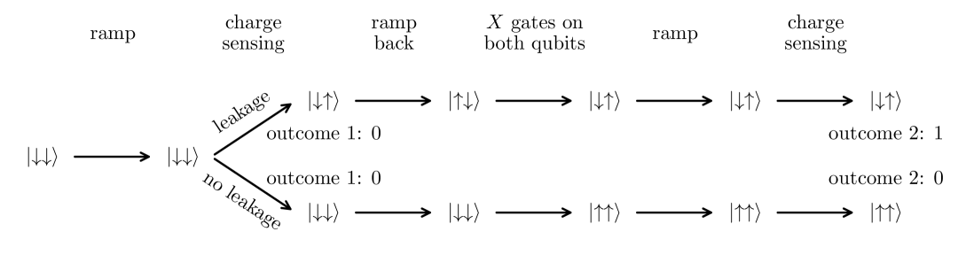
Now, we propose a leakage-detection experiment, which we first present by assuming that all other error probabilities are zero. Then, we list a set of experiments, including the leakage detection experiment, that can be used to estimate the error probabilities , , , and self-consistently. The leakage-detection experiment is summarized in Fig. S7. First, the state is prepared and spin-to-charge conversion is performed. Then the charge configuration is measured during which leakage is induced by the measurement with probability . The outcome of this charge measurement is 0, corresponding to the charge sector. Next, charge-to-spin conversion is performed and gates are applied to both of the spins. The resulting state after the gates is if leakage occurred and otherwise. Upon measuring these states again using spin-to-charge conversion and charge sensing, the outcome is if leakage occurred during the first measurement and otherwise. Therefore, leakage can be detected using this experiment.
Now, we show that this procedure can also be used to estimate the probability of leakage in the presence of the other error mechanisms listed above. The probabilities of the the four possible combinations of outcomes are
| (S61a) | ||||
| (S61b) | ||||
| (S61c) | ||||
| (S61d) | ||||
up to first order in the small error parameters , , , and . Leakage is then given by . Apparently, the error parameters and can also be estimated using this leakage-detection experiment. In order to estimate the remaining two error parameters and , two additional experiments need to be performed: (1) the state is prepared; (2) the state is prepared. Then, the prepared states are measured using spin-to-charge conversion and charge sensing. The outcome probabilities of these experiments are
| (S62a) | ||||
| (S62b) | ||||
| (S62c) | ||||
| (S62d) | ||||
Here, the subscripts and arguments indicate the outcomes and the prepared states respectively. Combining Eqs. (S61) and (S62), we have 5 independent equations, which allow us to estimate all of the error parameters.