Bandit based Dynamic Candidate Edge Selection in Solving Traveling Salesman Problems

Abstract

Algorithms designed for routing problems typically rely on high-quality candidate edges to guide their search, aiming to reduce the search space and enhance the search efficiency. However, many existing algorithms, like the classical Lin-Kernighan-Helsgaun (LKH) algorithm for the Traveling Salesman Problem (TSP), often use predetermined candidate edges that remain static throughout local searches. This rigidity could cause the algorithm to get trapped in local optima, limiting its potential to find better solutions. To address this issue, we propose expanding the candidate sets to include other promising edges, providing them an opportunity for selection. Specifically, we incorporate multi-armed bandit models to dynamically select the most suitable candidate edges in each iteration, enabling LKH to make smarter choices and lead to improved solutions. Extensive experiments on multiple TSP benchmarks show the excellent performance of our method. Moreover, we employ this bandit-based method to LKH-3, an extension of LKH tailored for solving various TSP variant problems, and our method also significantly enhances LKH-3’s performance across typical TSP variants.

1 Introduction

The Traveling Salesman Problem (TSP) is a classic NP-hard combinatorial optimization problem. Given an undirected complete graph where the distance between each pair of vertices (i.e., cities) is known, TSP aims to find the shortest path that starts from a starting city, passes each city exactly once, and then returns to the starting city. As the basic problem of many routing problems [1, 2, 3, 4, 5, 6], TSP also has many practical applications [7, 8].

Heuristic algorithms are known to be most efficient for solving the TSP, and they can be divided into two categories: global search and local search. Global search methods [9] attempt to explore a wide solution space with a global perspective incorporating entropy in individual selection and partial crossover which are impressive in genetic algorithm [10, 11]. However, it is hard and time-consuming for them to tackle super-large instances with huge solution spaces. Local search methods always maintain the current solution and explore its neighborhood space, which are efficient and suitable for instances with various scales. In this paper, we mainly focus on local search methods, among which the Lin-Kernighan-Helsgaun (LKH) [12] algorithm is one of the most representative and best-performing methods.

The LKH algorithm is an outstanding method among the Lin-Kernighan (LK) [13] series that collects some promising edges in the candidate sets of each city during initialization. When using the local search operators, such as $k$-opt, to adjust the current solution, the LK-based algorithms restrict the new edges to be added to belong to the candidate sets. Therefore, the algorithm performance heavily depends on the quality of the candidate edges. LKH proposes an effective metric called $\alpha$-value calculated based on a 1-tree structure to select the candidate edges [14], resulting in its excellent performance.

However, the candidate edges in LKH are generally predetermined in the initialization stage and then keep unchanged during the searching process. Therefore, the content of each city’s candidate edges is relatively fixed, and LKH only associates each city with about a fixed number of candidate edges (5 by default). Although the $\alpha$-value is promising in evaluating the quality of the edges, once some crucial edges in the optimal solution are missed by the collected candidate edges, it is hard for LKH to reach the global optimum. Simply enlarging the candidate sets allows the algorithm to consider more edges, which, however, reduces the efficiency significantly and may also contain some low-quality edges to mislead the search directions.

In this paper, we propose a novel method based on reinforcement learning to improve the LKH algorithm, helping it select the candidate edges more smartly and flexibly, providing more edges the opportunity to serve as candidate edges. Specifically, we first expand the candidate sets of each city to a larger size and then select a subset of edges from the candidate sets to serve as candidate edges during each iteration. We associate each city with a multi-armed bandit (MAB), where each arm corresponds to an edge in its enlarged candidate set and is associated with an evaluation value, denoted as $M$-value. The $M$-value of an arm indicates the benefit of selecting it as a candidate edge. The bandit models can learn from the searching process and update the $M$-values. In each iteration of the algorithm, the bandit models recommend appropriate candidate edges for the local search.

Moreover, we employ three different strategies for selecting the candidate edges, i.e., the arms of the bandit. The first strategy applies the $\epsilon$-greedy method to trade-off exploration and exploitation, while the other two make the selection greedily based on the $M$-values and $\alpha$-values, respectively. The three strategies are used cooperatively during the search to improve the robustness.

We apply our proposed method to LKH, denoting the resulting algorithm as Bandit-based LKH (bandLKH). Our method expands the searching space, providing higher flexibility for the search, assisting the LKH algorithm in escaping local optima and finding better solutions. We compare bandLKH with the LKH baseline, as well as VSR-LKH [15] and NeuroLKH [16], two representative learning-based algorithms. Extensive experiments in various benchmarks show the superiority of bandLKH over LKH, VSR-LKH, and NeuroLKH. In particular, our method exhibits better performance and robustness than simply enlarging the candidate sets in LKH. The results indicate that our MAB method can effectively and smartly suggest high-quality edges and ignore low-quality ones.

We further apply our MAB method to the LKH-3 algorithm [17], an extension of LKH that can solve many TSP variant problems efficiently. The resulting algorithm is denoted as bandLKH-3. We select two representative variant problem called Multiple Traveling Salesmen Problem (MTSP) and Capacitated Vehicle Routing Problem (CVRP), and compare our bandLKH-3 with LKH-3. The results show that our method can also significantly improve LKH-3 in MTSP and CVRP, indicating its excellent generalization capability.

The main contributions of this paper are as follows.

• We identified relatively rigid designs in the LKH algorithm, i.e., the candidate edges for each city are relatively fixed. We construct MAB models to select high-quality candidate edges adaptively during the searching process from enlarged candidate sets. We propose three policies to choose candidates coordinately and a framework to train and utilize the MAB models. Our proposed methods and framework can be applied to other heuristic algorithms for routing problems needing to select candidate edges.

• We compare bandLKH with LKH as well as representative learning-based algorithms for TSP on various benchmarks. We also generalize our method to LKH-3, which is an extension version of LKH for various TSP variants. Extensive experiments show the excellent performance and generalization capability of our method in TSP and its variant problems, MTSP and CVRP.

2 Problem Definition

In this section, we present the definition of the involved problems, including the Traveling Salesman Problem (TSP), the Multiple TSP (MTSP), and the Capacitated Vehicle Routing Problem (CVRP).

2.1 Traveling Salesman Problem

Given an undirected complete graph G(V,E), V is made up of cities in G numbered 1, 2, …, n and E contains all pairwise edges such as edge between city i and j presented by (i, j) which has its cost d(i,j). The aim is to find an hamiltonian circuit with a minimum total cost caculated by $\sum_{i=1}^{n-1}(d(i,i+1))+d(n,1)$.

2.2 Multiple TSP

In the MTSP, a set of $m$ salesmen (or vehicles) are available to visit a set of $n$ cities and each salesman starts and ends their route at a designated depot, with each city needing to be visited exactly once by one of the salesmen. Let $S=\{1,2,\ldots,m\}$ be the set of salesmen and $C=\{1,2,\ldots,n\}$ be the set of cities. $T_{1},T_{2},\ldots,T_{m}$ are composed of $m$ subsets $C_{1},C_{2},\ldots,C_{m}$ in $C$. The goal is to minimize $\sum_{k=1}^{m}\sum_{(i,j)\in T_{k}}d(i,j)$.

2.3 Capacitated Vehicle Routing Problem

In the CVRP, define m homogeneous fleets serving n cities have a max capacity $c$ which could not be exceeded in each vehicle. Due to capacity, n cities are divided into m exclusive parts represented by $T_{1},T_{2},\ldots,T_{m}$ besides common starting and ending cities. Each customer in $T_{i}$ is visited exactly once by one of the vehicles and common cities can be visited many times. The total distance traveled by all vehicles, $\sum_{k=1}^{m}\sum_{(i,j)\in T_{k}}d(i,j)$, is minimized.

3 Related Work

In this section, we first review some related studies that solve TSP with learning-based methods and then briefly introduce some key components used in LKH.

3.1 Learning-based Methods

Recently, the application of learning-based methods, such as reinforcement learning and deep learning, for combinatorial optimization problems has become a highlight of research. TSP has even become a touchstone and one of the most popular problems for learning-based methods.

Learning-based methods for TSP can be roughly divided into two categories depending on whether deep learning is adopted. Actually, most learning-based methods try to apply deep learning methods for TSP solving. Typical methods include deep reinforcement learning and supervised learning. For instance, some studies design or apply novel deep learning structures for solving TSP, such as the multi-pointer Transformer architecture called Pointerformer [18] and the hierarchical deep reinforcement learning framework [19]. Some studies train neural networks to automate the heuristic design, such as the Ant Colony Optimization and $k$-opt [20, 21, 22] heuristics. The NeuroLKH algorithm utilizes a Sparse Graph Network to select candidate edges for LKH [16], showing excellent performance in instances with less than 6,000 cities. Aigerim propose a hybrid model combining an attention-based encoder and a Long Short-Term Memory (LSTM) decoder addressing the challenge of routing a heterogeneous fleet. [23]. Bresson trains via deep reinforcement learning, effectively addresses the combinatorial optimization challenges of the TSP[24]. GRLOS-M uses Graph Neural Networks to improve Adaptive Large Neighbourhood Search [25]. There are also some other famous models and algorithms using deep learning for TSP, such as S2V-DQN [26], POMO [27], GLOP [28], etc.

The deep learning-based methods provide many new and interesting perspectives for solving TSP. However, they are usually hard to scale to large instances with tens of thousands of cities. The other category of method usually uses traditional reinforcement learning to accumulate the learning information in tables and use them to guide the search.traditional reinforcement learning plays an important part role in TSP. Mazyavkina summarized the TSP problem based on reinforcement learning[29]. For example, the Ant-Q [30] and Q-ACS [31] replace the pheromone in the ant colony algorithm with the Q-table in the Q-learning algorithm. The RMGA algorithm [32] uses reinforcement learning to construct mutation individuals in genetic algorithms. RLHEA combines Q-learning method with hybrid evolutionary algorithm for routing problem [33]. Moreover, the VSR-LKH [15] algorithm combines typical reinforcement learning methods with LKH, altering and reordering the candidate edges, showing excellent performance in TSP. Reinforcement learning also has many opportunities in solving stochastic dynamic vehicle routing problem [34].

Our proposed method uses MAB models to select and adjust candidate edges during the local search. Compared to NeuroLKH and VSR-LKH, which also select and determine the candidate edges before the local search process, our method provides more opportunity for other promising edges to be contained in candidate sets, allowing the algorithm to effectively solve instances with various scales and structures.

3.2 Key Components in LKH

3.2.1 The $\alpha$-value

Candidate edges are very important for LK-based local search algorithms since they decide the new edges that can be added to the maintained solution. LKH proposes the $\alpha$-value for evaluating the edges and selecting the candidate edges. The $\alpha$-value is calculated based on a 1-tree structure [14], a variant of the spanning tree. Given a graph $G=(V,E)$, for any vertex $v\in V$, we can generate a 1-tree by first constructing a spanning tree on $V\backslash\{v\}$ and then combining it with two edges from $E$ incident to $v$. The minimum 1-tree is the 1-tree with the minimum length, i.e., the total length of its edges. We denote $L(T)$ as the length of the minimum 1-tree, which is obviously a lower bound of the length of the shortest TSP tour. Moreover, we denote $L(T(i,j))$ as the length of the minimum 1-tree containing edge $(i,j)$. The $\alpha$-value of edge $(i,j)$ is calculated as follows.

$$\alpha(i,j)=L(T(i,j))-L(T).$$ (1)

To further enhance the performance of $\alpha$-values, LKH applies the method of adding penalties [35] to vertices to obtain a tighter lower bound.

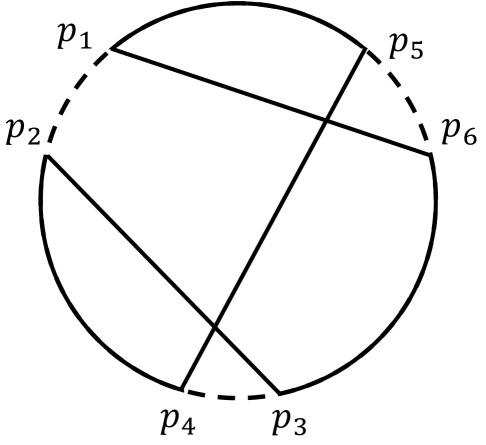
(a) Sequential 3-opt

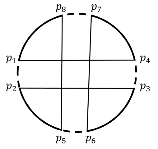
(b) Non-sequential 4-opt

Figure 1: Examples of sequential and non-sequential $k$-opt moves.

3.2.2 Search Operators

The core search operator in LKH is the famous $k$-opt method, which replaces $k$ edges in the current solution with $k$ new edges based on the eject chain method. That is, remove $k$ edges in the tour and attempt to rearrange the order of connections among these points to find a better solution. The $k$-opt operator in LKH contains two categories, sequential and non-sequential moves, as shown in Figure 1. The dashed line is the edge that is about to be disconnected. The sequential move starts from a starting point, e.g., $p_{1}$, alternatively selects the edges to be removed, e.g., $(p_{1},p_{2})$, $(p_{3},p_{4})$ and $(p_{5},p_{6})$, and edges to be added, e.g., $(p_{2},p_{3})$ and $(p_{4},p_{5})$, and guarantees that after selecting each edge to be removed, connecting its endpoint, e.g., $p_{4}$ and $p_{6}$, back to the starting point leads to a feasible TSP tour. Therefore, the sequential move can be stopped once an improvement is found, and the non-sequential move cannot. The non-sequential move combines two distinct infeasible $k$-opt moves to form a feasible tour, as shown in Figure 1(b). It is a supplement of the sequential move, exploring additional search space that sequential moves cannot reach.

In summary, the search operators in LKH are encapsulated in the LinKernighan() function, which is an important part of executing LK algorithm [13], following the guidance of the candidate edges to find moves that can improve the current solution. LinKernighan() finally returns a local optimal solution that cannot be improved by any search operators with the candidate edges. For the detailed implementations of the LinKernighan() function, we referred to [12].

4 Method

This section presents our proposed bandLKH algorithm. We first introduce our method of using multi-armed bandits (MAB) to select and recommend candidate edges for the local search algorithm, then introduce the main framework of bandLKH, and finally introduce the method for calculating the rewards and updating the bandit models.

4.1 Candidate Edges Selection

As described in the introduction, our proposed MAB models select high-quality candidate edges from the enlarged candidate sets. Note that LKH restricts the maximum edges contained in each candidate set using a constant parameter $C_{max}$, whose default value is 5. Such a default value fits well with the algorithm, as a smaller value significantly reduces the search ability, and a larger value may contain low-quality edges and reduce the search efficiency. However, the restriction of $C_{max}=5$ may also miss some promising edges. Therefore, we propose to enlarge each candidate set to a larger size (setting $C_{max}=7$ by default), allowing more edges to serve as candidate edges, and further use an MAB to ignore low-quality edges and select appropriate edges in each candidate set.

In the experiments, we perform an empirical analysis to evaluate the benefit of the expansion of candidate sets and a comparison showing that using our MAB to select candidate edges from the enlarged candidate sets is more robust and effective than regarding all edges in the enlarged candidate sets as candidate edges directly, indicating the excellent performance of our method.

In the following, we first introduce the proposed MAB model and then the method of pulling the arms in the bandit models.

4.1.1 The MAB Model

Given the enlarged candidate set of each city, directly regarding all its edges as candidate edges will significantly reduce the algorithm efficiency and may contain some low-quality edges. Thus, we need to select some appropriate ones from each enlarged candidate set. Such a task background shares similarities with the MAB model, which also needs to perform selections from multiple candidates and lacks prior knowledge for selecting the best ones in each step. There are also some differences between them, i.e., the candidate set needs to produce multiple candidate edges and the MAB model usually only pulls one arm per step. Therefore, we establish the task as a variant MAB model [36], which pulls multiple arms each time. Specifically, we associate each city with an MAB, where each arm corresponds to an edge in its enlarged candidate set, and pulling each arm corresponds to select the corresponding edge as a candidate edge.

For each arm in each MAB, we assign it an evaluation value, denoted as $M$-value. The $M$-values are initialized to be 0 in the beginning. The larger the $M$-value of an arm, the more the benefit of selecting it as a candidate edge. Our MAB models can learn from the search process and adjust the $M$-values, using them to recommend appropriate candidate edges for the local search algorithm.

4.1.2 Methods for Pulling the Arms

In our method, each MAB needs to pull $N_{arm}$ (5 by default equals to $C_{max}$ of LKH) arms per calling and recommends $N_{arm}$ corresponding candidate edges to participate in the local search process. We design three methods for selecting the arms to be pulled, denoted as $\epsilon$-greedy, $M$-greedy, and $\alpha$-greedy, respectively. Their formal descriptions are as follows.

• $\epsilon$-greedy randomly explores the edges in the enlarged candidate set with a probability of $\epsilon$ ($0<\epsilon<1$) and makes a greedy selection preferring edges with larger $M$-values with a probability of $1-\epsilon$.

• $M$-greedy selects $N_{arm}$ edges with the largest $M$-values greedily among each enlarged candidate set.

• $\alpha$-greedy selects $N_{arm}$ edges with the largest $\alpha$-values greedily among each enlarged candidate set.

The above three methods are used alternatively during the search process. Actually, the $M$-values and $\alpha$-values share similarities and differences. Both of them serve as metrics of the edges. The $\alpha$-values are predetermined before the local search process, evaluating the quality of the edges with a global perspective. In contrast, the $M$-values are continuously learned and updated during the local search process. We believe that these two metrics are complementary in evaluating and selecting the candidate edges, and the utilization of the $M$-greedy and $\alpha$-greedy methods combine their complementarity. Moreover, the $\epsilon$-greedy allows the MAB reinforcement learning models to trade-off exploration and exploitation. Experimental results also demonstrate that the combination of the three methods can improve the robustness of the local search algorithm.

Given the $M$-values and $\alpha$-values of the edges, the parameter $\epsilon$, an integer $bandtype$ for determining the selection of the three methods, and the number of pulled arms per calling of MAB $N_{arm}$, Algorithm 1 shows a CallBandit() function that calls the MAB models to select the candidate edges for the local search algorithm. The set of all selected candidate edges is denoted as $E_{cand}$.

Input: $\epsilon$-greedy parameter: $\epsilon$, integer for determining the method: $bandtype$, number of pulled arms: $N_{arm}$

Output: Candidate edges $E_{cand}$

1 switch bandtype do

2    case 0 do select $E_{cand}$ by the $\epsilon$-greedy method;

3    case 1 do select $E_{cand}$ by the $M$-greedy method;

4    case 2 do select $E_{cand}$ by the $\alpha$-greedy method;

5   

6return $E_{cand}$;

Algorithm 1 CallBandit($\epsilon,bandtype,N_{arm}$)

4.2 Main Process of bandLKH

After establishing the MAB model and the method for selecting candidate edges, we summarize the main framework of bandLKH in this subsection, which is depicted in Algorithm 2. In the initialization stage (lines 1-5), the algorithm initializes the enlarged candidate sets, the $M$-values, and some information involved in the search process. During the local search process (lines 6-19), the algorithm first generates an initial solution $R$ by function ChooseInitialTour() in LKH (line 7) and then calls the MAB models by function CallBandit() (Algorithm 1) to select the candidate edges $E_{cand}$ (line 8). The selected $E_{cand}$ will be used to guide the LinKernighan() function, which performs the search operators introduced in Section 3.2.2 to improve $R$ to a local optimum (line 9). The $M$-values of the selected candidate edges will be updated according to the quality of the obtained local optimal solution (line 10). Moreover, if the best solution $R^{*}$ has not been improved for $T_{type}$ trials, the $bandtype$ will be changed (line 18) to try to use different arm selection methods to help the algorithm escape from local optima.

For the time complexity, the additional operations of bandLKH over LKH are the CallBandit and UpdateM functions. CallBandit sorts the enlarged candidate set with size $C_{max}$ (7 by default) of each city, costing a time complexity of $O(nC_{max}log(C_{max})$, where $n$ is the number of cities. UpdateM traverses the selected candidate edges once, costing a time complexity of $O(n)$. For the space complexity, bandLKH associates an $M$-value with each candidate city, costing a space complexity of $O(C_{max}n)$. Therefore, both the time and space complexities are of linear order and acceptable for large-scale problems.

In summary, the proposed bandLKH algorithm uses the MAB models to help select candidate edges for the local search process. The MAB models select the candidate edges referring to the evaluation values of the arms, i.e., $M$-values, and can learn from the searching process to update the $M$-values and recommend appropriate and high-quality candidate edges. The selected candidate edges can be used for various search operators in LKH encapsulated in the LinKernighan() function, including sequential and non-sequential moves.

Input: A TSP instance: $I$, enlarged size of candidate sets: $C_{max}$, maximum number of trials: $MaxTrials$, the cut-off time: $MaxTime$, number of pulled arms: $N_{arm}$, maximum no-improvement trials for change $bandtype$: $T_{type}$, $\epsilon$-greedy parameter: $\epsilon$, incremental reward parameter: $\lambda$

Output: The best solution found for $I$: $R^{*}$

1 Initialize each enlarged candidate set containing $C_{max}$ edges based on $\alpha$-values;

2 Initialize length of the best solution $L(R^{*})\leftarrow+\infty$;

3 Initialize the number of no-improvement trials $t\leftarrow 0$;

4 Initialize $bandtype\leftarrow 0$;

5 Initialize the $M$-values to 0;

6 for $i\leftarrow 1:MaxTrials$ do

7    $R\leftarrow$ ChooseInitialTour();

8    $E_{cand}\leftarrow$ CallBandit($\epsilon,bandtype,N_{arm}$);

9    $R\leftarrow$ LinKernighan($I,R,E_{cand}$);

10    UpdateM($E_{cand},R,R^{*},\lambda$);

11    if $L(R)<L(R^{*})$ then

12       $R^{*}\leftarrow R$;

13       $t\leftarrow 0$;

14      

15   else

16       $t\leftarrow t+1$;

17       if $t\geq T_{type}$ then

18          $t\leftarrow$ 0;

19          $bandtype\leftarrow(bandtype+1)\%3$;

20         

21      

22   if running time $>MaxTime$ then break;

23   

24return $R^{*}$;

Algorithm 2 bandLKH

4.3 Update the $M$-values with Rewards

To update the evaluation values, i.e., $M$-values, of the arms in our MAB models, we need to design the reward functions for evaluating the benefit of pulling the arms, i.e., selecting the corresponding candidate edges. Suppose $R^{*}$ is the best solution found during the search process and $R$ is the solution obtained by the function LinKernighan() based on the selected candidate edges in the current trial. A simple and straightforward reward function is designed as follows.

$$r(R,R^{*})=L(R^{*})-L(R).$$ (2)

Given the above reward function, the function UpdateM() updates the $M$-value of each selected candidate edge $(i,j)\in E_{cand}$ in an incremental manner by the following equation.

$$M(i,j)=(1-\lambda)\cdot M(i,j)+\lambda\cdot r(R,R^{*}),$$ (3)

where $0<\lambda<1$ is the incremental reward parameter.

5 Experiment

In this section, we first make a detailed comparison between bandLKH and LKH (version 2.0.10) to evaluate the performance of our proposed new algorithm. We also compare bandLKH with representative learning-based methods, including the deep learning-based NeuroLKH algorithm [16] and the traditional reinforcement learning-based VSR-LKH algorithm [15]. We further present ablation studies to evaluate the efficacy of components in bandLKH and provide further insights.

Finally, we apply our method to LKH-3 [17], an extension of LKH that can solve many TSP variants. The resulting solver is called bandLKH-3. We select two representative variants of TSP: the Multiple Traveling Salesmen Problem (MTSP), where the cities are visited by $m$ salesmen, and the goal is to minimize their total traveling distance, and the Capacitated Vehicle Routing Problem (CVRP), which regards the salesmen and cities as vehicles with capacities and customers with demands, and the goal is to minimize the total traveling distance of the vehicles while ensuring that each customer’s demand is satisfied and the total demand does not exceed the capacity of any vehicle. We compare bandLKH-3 with LKH-3 in solving MTSP and CVRP and evaluate the generalization capability of our method.

Table 1: Detailed comparison results of bandLKH and LKH. The best results appear in bold.

Instance	BKS	LKH						bandLKH
		Success	Best (%)	Average (%)	Trials	Time (s)		Success	Best (%)	Average (%)	Trials	Time (s)
gr137	69853	10/10	69853 (0.0000)	69853 (0.0000)	1.0	0.01		9/10	69853 (0.0000)	69865.7 (0.0182)	18.9	0.01
ch150	6528	9/10	6528 (0.0000)	6528.5 (0.0077)	60.1	0.05		10/10	6528 (0.0000)	6528 (0.0000)	23.3	0.08
kroB150	26130	2/10	26130 (0.0000)	26131.6 (0.0061)	128.4	0.24		10/10	26130 (0.0000)	26130 (0.0000)	54.1	0.21
si175	21407	7/10	21407 (0.0000)	21407.3 (0.0014)	105.9	6.15		9/10	21407 (0.0000)	21407.1 (0.0005)	35.3	4.95
rat195	2323	9/10	2323 (0.0000)	2323.5 (0.0215)	55.0	0.15		10/10	2323 (0.0000)	2323 (0.0000)	14.8	0.19
gr229	134602	2/10	134602 (0.0000)	134613.2 (0.0083)	203.1	0.20		10/10	134602 (0.0000)	134602 (0.0000)	25.9	0.14
pr299	48191	9/10	48191 (0.0000)	48194.3 (0.0068)	51.7	0.36		10/10	48191 (0.0000)	48191 (0.0000)	21.6	0.68
lin318	42029	4/10	42029 (0.0000)	42085.4 (0.1342)	249.3	0.55		9/10	42029 (0.0000)	42040.4 (0.0271)	53.0	0.34
gr431	171414	3/10	171414 (0.0000)	171499.2 (0.0497)	347.0	1.73		10/10	171414 (0.0000)	171414 (0.0000)	73.7	2.26
d493	35002	2/10	35002 (0.0000)	35003.6 (0.0046)	419.3	2.62		10/10	35002 (0.0000)	35002 (0.0000)	28.2	0.98
si535	48450	7/10	48450 (0.0000)	48451.1 (0.0023)	311.6	21.28		9/10	48450 (0.0000)	48450.3 (0.0006)	138.9	31.98
rat575	6773	2/10	6773 (0.0000)	6773.8 (0.0118)	526.9	2.32		6/10	6773 (0.0000)	6773.4 (0.0059)	392.5	4.93
gr666	294358	5/10	294358 (0.0000)	294417 (0.0200)	459.8	2.41		6/10	294358 (0.0000)	294393.7 (0.0121)	372.9	10.01
pr1002	259045	8/10	259045 (0.0000)	259045.6 (0.0002)	549.0	3.13		10/10	259045 (0.0000)	259045 (0.0000)	90.7	2.83
u1060	224094	5/10	224094 (0.0000)	224107.5 (0.0060)	663.3	84.17		10/10	224094 (0.0000)	224094 (0.0000)	44.4	22.00
vm1084	239297	3/10	239297 (0.0000)	239372.6 (0.0316)	824.1	32.98		8/10	239297 (0.0000)	239307.4 (0.0043)	323.9	26.51
pcb1173	56892	4/10	56892 (0.0000)	56895 (0.0053)	844.0	3.92		8/10	56892 (0.0000)	56893 (0.0018)	418.4	9.79
d1291	50801	5/10	50801 (0.0000)	50840 (0.0768)	995.4	27.44		10/10	50801 (0.0000)	50801 (0.0000)	192.2	14.74
rl1304	252948	3/10	252948 (0.0000)	253156.4 (0.0824)	1170.0	12.48		10/10	252948 (0.0000)	252948 (0.0000)	572.1	27.38
rl1323	270199	6/10	270199 (0.0000)	270219.6 (0.0076)	718.8	9.63		8/10	270199 (0.0000)	270204.4 (0.0020)	576.9	23.75
nrw1379	56638	6/10	56638 (0.0000)	56640 (0.0035)	759.3	8.87		6/10	56638 (0.0000)	56639.6 (0.0028)	928.0	35.27
fl1400	20127	0/10	20164 (0.1838)	20165.5 (0.1913)	1400.0	113.30		6/10	20127 (0.0000)	20141.8 (0.0735)	721.0	219.18
fl1577	22249	0/10	22254 (0.0225)	22260.6 (0.0521)	1577.0	1172.10		9/10	22249 (0.0000)	22249.5 (0.0022)	614.9	1920.79
vm1748	336556	9/10	336556 (0.0000)	336557.3 (0.0004)	1007.9	12.69		10/10	336556 (0.0000)	336556 (0.0000)	146.4	9.99
u1817	57201	1/10	57201 (0.0000)	57251.1 (0.0876)	1817.0	74.19		1/10	57201 (0.0000)	57237.3 (0.0635)	1750.3	260.67
rl1889	316536	0/10	316549 (0.0041)	316549.8 (0.0044)	1889.0	61.40		10/10	316536 (0.0000)	316536 (0.0000)	236.5	35.56
d2103	80450	0/10	80471 (0.0261)	80505.7 (0.0692)	2103.0	67.07		7/10	80450 (0.0000)	80451 (0.0012)	1084.0	306.06
u2152	64253	3/10	64253 (0.0000)	64287.7 (0.0540)	1614.0	73.81		8/10	64253 (0.0000)	64264.4 (0.0177)	793.6	135.39
pcb3038	137694	4/10	137694 (0.0000)	137701.2 (0.0052)	2078.6	69.56		5/10	137694 (0.0000)	137700.7 (0.0049)	2081.1	275.37
fl3795	28772	4/10	28772 (0.0000)	28783.2 (0.0389)	2998.1	423.94		5/10	28772 (0.0000)	28778.5 (0.0226)	3012.3	2437.03
fnl4461	182566	9/10	182566 (0.0000)	182566.5 (0.0003)	923.1	31.05		10/10	182566 (0.0000)	182566 (0.0000)	153.4	37.02
rl5915	565530	1/10	565530 (0.0000)	565621.5 (0.0162)	5915.0	242.05		3/10	565530 (0.0000)	565564.4 (0.0061)	4863.8	1663.58
rl5934	556045	0/10	556172 (0.0228)	556377.6 (0.0598)	5934.0	305.02		8/10	556045 (0.0000)	556063.2 (0.0033)	3472.1	1607.18
xmc10150	28387	0/5	28388 (0.0035)	28388.8 (0.0063)	10000.0	832.77		0/5	28389 (0.0070)	28390.8 (0.0134)	10000.0	4279.32
fi10639	520527	0/5	520534 (0.0013)	520562.8 (0.0069)	10000.0	844.41		0/5	520539 (0.0023)	520564.2 (0.0071)	10000.0	4636.34
rl11849	923288	1/5	923288 (0.0000)	923360.2 (0.0078)	9257.4	947.41		1/5	923288 (0.0000)	923323.6 (0.0039)	8532.0	3633.09
usa13509	19982859	0/5	19982874 (0.0001)	19983306.2 (0.0022)	10000.0	1111.75		0/5	19983027 (0.0008)	19983277.2 (0.0021)	10000.0	6300.91
xvb13584	37083	1/5	37083 (0.0000)	37087.2 (0.0113)	8251.2	1053.74		0/5	37086 (0.0081)	37090.4 (0.0200)	10000.0	5740.31
brd14051	469385	0/5	469395 (0.0021)	469397.4 (0.0026)	10000.0	1789.55		0/5	469412 (0.0058)	469460.6 (0.0161)	10000.0	8240.87
mo14185	427377	0/5	427381 (0.0009)	427402.6 (0.0060)	10000.0	1408.07		0/5	427380 (0.0007)	427385.8 (0.0021)	10000.0	6173.50
xrb14233	45462	0/5	45466 (0.0088)	45468.4 (0.0141)	10000.0	1376.69		1/5	45462 (0.0000)	45465 (0.0066)	10000.0	6659.30
ho14473	177092	0/5	177161 (0.0390)	177182.6 (0.0512)	332.2	43362.26		0/5	177117 (0.0141)	177138 (0.0260)	402.8	43336.19
d15112	1573084	0/5	1573202 (0.0075)	1573242.6 (0.0101)	10000.0	2109.11		0/5	1573288 (0.0130)	1573318.8 (0.0149)	10000.0	9560.62
it16862	557315	0/5	557319 (0.0007)	557336 (0.0038)	10000.0	6012.14		0/5	557319 (0.0007)	557332.4 (0.0031)	8975.0	39870.58
xia16928	52850	1/5	52850 (0.0000)	52853.2 (0.0061)	10000.0	1673.98		1/5	52850 (0.0000)	52852 (0.0038)	10000.0	9295.23
pjh17845	48092	0/5	48093 (0.0021)	48100.4 (0.0175)	10000.0	1739.08		0/5	48093 (0.0021)	48095.6 (0.0075)	10000.0	10022.94
d18512	645238	0/5	645263 (0.0039)	645268.8 (0.0048)	10000.0	2668.68		0/5	645353 (0.0178)	645424.4 (0.0289)	10000.0	10513.63
frh19289	55798	0/5	55800 (0.0036)	55806.8 (0.0158)	10000.0	1836.78		0/5	55804 (0.0108)	55808.8 (0.0194)	10000.0	11312.59
fnc19402	59287	0/5	59303 (0.0270)	59308.6 (0.0364)	10000.0	1823.40		0/5	59295 (0.0135)	59298.6 (0.0196)	10000.0	9574.85
ido21215	63517	0/5	63525 (0.0126)	63533.6 (0.0261)	10000.0	2161.70		0/5	63519 (0.0031)	63525.6 (0.0135)	10000.0	14603.81
fma21553	66527	0/5	66529 (0.0030)	66540.4 (0.0201)	10000.0	2102.46		1/5	66527 (0.0000)	66534.8 (0.0117)	10000.0	11584.06
vm22775	569288	0/5	569299 (0.0019)	569308.6 (0.0036)	10000.0	7171.50		0/5	569290 (0.0004)	569308.8 (0.0037)	10000.0	20219.20
lsb22777	60977	0/5	60981 (0.0066)	60989 (0.0197)	10000.0	2625.61		0/5	60978 (0.0016)	60983.8 (0.0112)	10000.0	15632.94
xrh24104	69294	0/5	69300 (0.0087)	69304.2 (0.0147)	10000.0	2303.96		0/5	69297 (0.0043)	69303.2 (0.0133)	10000.0	16508.96
sw24978	855597	0/5	855599 (0.0002)	855628 (0.0036)	10000.0	2807.11		0/5	855602 (0.0006)	855611.8 (0.0017)	10000.0	17463.64
bbz25234	69335	0/5	69343 (0.0115)	69349.8 (0.0213)	10000.0	2938.86		0/5	69340 (0.0072)	69346.2 (0.0162)	10000.0	21084.39
irx28268	72608	0/5	72614 (0.0083)	72622 (0.0193)	10000.0	2979.10		1/5	72608 (0.0000)	72610.2 (0.0030)	10000.0	17642.29
fyg28534	78562	0/5	78571 (0.0115)	78574.6 (0.0160)	10000.0	2941.72		0/5	78568 (0.0076)	78573.2 (0.0143)	10000.0	21597.03
icx28698	78087	0/5	78100 (0.0166)	78106.8 (0.0254)	10000.0	3237.22		0/5	78093 (0.0077)	78104.4 (0.0223)	10000.0	22079.87
ird29514	80353	0/5	80366 (0.0162)	80374.8 (0.0271)	10000.0	3052.62		0/5	80380 (0.0336)	80392.4 (0.0490)	10000.0	24177.14
pla33810	66048945	0/5	66061689 (0.0193)	66065656.2 (0.0253)	3000.0	25030.56		0/5	66052269 (0.0050)	66062745 (0.0209)	1442.4	29411.21
pla85900	142382641	0/5	142455345 (0.0511)	142457070.8 (0.0523)	3000.0	9270.29		0/5	142404864 (0.0156)	142411899.2 (0.0205)	3000.0	25842.53
Average Gap (%)	-	-	0.0085	0.0249	-	-		-	0.0030	0.0107	-	-

Table 2: Summarized comparison results of bandLKH and learning-based methods, VSR-LKH and NeuroLKH. The best results appear in bold.

Indicator	bandLKH	VSR-LKH	bandLKH	NeuroLKH_R	bandLKH	NeuroLKH_M
$Win_{best}$	2	0	8	0	5	0
$Win_{avg}$	13	9	22	8	13	9
$Gap_{best}$	0.0000%	0.0027%	0.0000%	0.0215%	0.0000%	0.0803%
$Gap_{avg}$	0.0036%	0.0060%	0.0043%	0.0366%	0.0043%	0.0834%

Table 3: Summarized comparison results of bandLKH and its variants, bandLKH-no$\epsilon$, bandLKH-no$M$, and bandLKH-no$\alpha$. The best results appear in bold.

Indicator	bandLKH	bandLKH-no$\epsilon$	bandLKH	bandLKH-no$M$	bandLKH	bandLKH-no$\alpha$
$Win_{best}$	0	0	0	0	2	0
$Win_{avg}$	12	7	6	12	28	4
$Gap_{best}$	0.0000%	0.0000%	0.0000%	0.0000%	0.0000%	0.0006%
$Gap_{avg}$	0.0036%	0.0044%	0.0036%	0.0057%	0.0036%	0.0076%

Table 4: Summarized comparison results between bandLKH with LKH-$N_{arm}$ and LKH-$C_{max}$. The best results appear in bold.

Indicator	bandLKH	LKH-$C_{max}$
$Win_{best}$	1	0
$Win_{avg}$	19	12
$Gap_{best}$	0.0000%	0.0001%
$Gap_{avg}$	0.0036%	0.0057%

Table 5: Detailed comparison of LKH3 and bandLKH-3 on CVRP. The best results appear in bold.

	LKH-3					bandLKH-3
Instance	Best	Average	Trials	Time(s)		Best	Average	Trials	Time(s)
X-n101-k25	27653	27717.4	10000.0	56.48		27591	27625	7393.0	19.872
X-n106-k14	26389	26482.2	10000.0	50.67		26386	26388.2	10000.0	61.72
X-n110-k13	14971	14971	1271.0	0.37		14971	14971	2048.0	0.698
X-n115-k10	12747	12754	5159.0	1.76		12747	12747	314.0	0.069
X-n120-k6	13332	13351.5	6011.0	3.03		13340	13374.4	10000.0	12.692
X-n125-k30	55736	55880.4	10000.0	161.35		55675	55812.2	10000.0	167.218
X-n129-k18	28958	29034.4	10000.0	38.26		28957	29049.4	10000.0	47.892
X-n134-k13	10933	10985.2	10000.0	39.71		10918	10964.4	10000.0	50.12
X-n139-k10	13590	13590	1167.0	0.33		13612	13641	10000.0	16.549
X-n143-k7	15726	15774.4	10000.0	24.08		15726	15789.6	10000.0	29.478
X-n148-k46	43448	43448	5442.0	5.01		43594	43706.8	10000.0	50.921
X-n153-k22	21254	21290.6	10000.0	71.11		21247	21275.4	10000.0	87.463
X-n157-k13	16876	16885	5339.0	3.22		16876	16876	2229.0	1.007
X-n162-k11	14138	14196.75	8457.2	8.98		14153	14167.4	10000.0	15.617
X-n167-k10	20637	20752	10000.0	30.91		20610	20742.4	10000.0	34.993
X-n172-k51	45733	45830.2	10000.0	58.51		45637	45806.2	10000.0	65.726
X-n176-k26	48076	48217.8	10000.0	157.76		47895	48041.4	10000.0	186.436
X-n181-k23	25572	25628	10000.0	18.02		25576	25626.4	10000.0	24.256
X-n186-k15	24279	24304	10000.0	52.09		24212	24394.2	10000.0	55.446
X-n190-k8	17041	17197.4	10000.0	40.08		17031	17173.6	10000.0	47.873
X-n195-k51	44322	44432	10000.0	51.65		44480	44527.4	10000.0	69.822
X-n200-k36	58882	58934.4	10000.0	155.41		58819	58901.4	10000.0	214.636
X-n204-k19	19699	19746.4	10000.0	22.49		19610	19696.4	10000.0	28.873
X-n209-k16	30855	31031.8	10000.0	44.07		31043	31117	10000.0	50.978
X-n214-k11	11138	11252.2	10000.0	107.32		11089	11189.2	10000.0	116.901
X-n219-k73	117613	117675.2	10000.0	45.03		117613	117685.4	10000.0	1142.35
X-n223-k34	40704	40804.6	10000.0	59.50		40688	40799.8	10000.0	71.578
X-n228-k23	25782	25906.6	10000.0	69.01		25806	25869.8	10000.0	73.489
X-n233-k16	19365	19465.2	10000.0	16.56		19313	19411.4	10000.0	22.386
X-n237-k14	27128	27266.8	10000.0	29.61		27050	27165.2	10000.0	36.486
X-n242-k48	83121	83468.8	10000.0	91.32		83197	83358	10000.0	107.912
X-n247-k47	37353	37487.8	10000.0	114.37		37290	37337.8	10000.0	155.195
X-n251-k28	38914	39040.4	10000.0	52.43		38812	39008	10000.0	67.16
X-n256-k16	19062	19207.4	10000.0	70.77		19000	19213.2	10000.0	78.19
X-n261-k13	26808	27075.2	10000.0	63.92		26948	27088.6	10000.0	89.908
X-n266-k58	75795	76074.6	10000.0	160.84		75948	76111	10000.0	194.644
X-n270-k35	35504	35566.8	10000.0	62.32		35506	35702.8	10000.0	75.149
X-n275-k28	21347	21418.4	10000.0	22.63		21347	21426	10000.0	26.471
X-n280-k17	33835	33921.6	10000.0	102.88		33725	33878	10000.0	130.435
X-n284-k15	20348	20640	10000.0	36.72		20401	20514.6	10000.0	38.847
X-n289-k60	96038	96238.8	10000.0	255.37		95983	96199.6	10000.0	298.468
X-n294-k50	47473	47637	10000.0	74.52		47508	47654.8	10000.0	97.423
X-n298-k31	34522	34776.6	10000.0	54.44		34431	34581.6	10000.0	67.207
X-n303-k21	21919	22008.2	10000.0	36.47		21906	22027.4	10000.0	40.758
X-n308-k13	26208	26266.6	10000.0	63.42		26022	26231	10000.0	64.52
X-n313-k71	95087	95197.2	10000.0	250.89		94880	94950.4	10000.0	294.031

Table 6: Detailed comparison of LKH3 and bandLKH-3 on CVRP (continued). The best results appear in bold.

	LKH-3					bandLKH-3
Instance	Best	Average	Trials	Time(s)		Best	Average	Trials	Time(s)
X-n317-k53	78389	78608.6	10000.0	78.26		78458	78679.6	10000.0	106.873
X-n322-k28	30228	30369.4	10000.0	72.03		30233	30263.6	10000.0	83.37
X-n327-k20	27887	28015.8	10000.0	58.75		28027	28078.8	10000.0	73.938
X-n331-k15	31488	31565	10000.0	30.20		31393	31608.8	10000.0	40.726
X-n336-k84	140006	140344.8	10000.0	231.94		140023	140283.4	10000.0	282.161
X-n344-k43	42502	42682.6	10000.0	78.53		42551	42720.2	10000.0	98.49
X-n351-k40	26261	26333.4	10000.0	102.05		26236	26308	10000.0	128.196
X-n359-k29	52210	52284.8	10000.0	106.94		52061	52329.8	10000.0	136.523
X-n367-k17	23163	23290	10000.0	48.84		23113	23240.4	10000.0	60.611
X-n376-k94	147877	147982.2	10000.0	77.43		147840	147953.2	10000.0	93.745
X-n384-k52	66514	66668	10000.0	136.75		66656	66833.2	10000.0	166.046
X-n393-k38	38633	38816	10000.0	76.18		38656	38772	10000.0	95.672
X-n401-k29	66619	66781.6	10000.0	241.04		66581	66720.4	10000.0	281.493
X-n411-k19	20083	20165.4	10000.0	76.96		19883	19950.8	10000.0	86.724
X-n429-k61	66136	66427.8	10000.0	108.46		66257	66419	10000.0	145.347
X-n439-k37	36656	36755.6	10000.0	21.44		36554	36642.4	10000.0	27.291
X-n449-k29	56523	56680.6	10000.0	318.24		56550	56697.8	10000.0	364.509
X-n459-k26	24559	24729.8	10000.0	108.59		24507	24681.8	10000.0	126.728
X-n469-k138	223805	224058.6	10000.0	419.96		223683	223783	10000.0	861.448
X-n480-k70	90205	90413	10000.0	133.73		90086	90233.4	10000.0	154.667
X-n491-k59	67539	67781.2	10000.0	304.39		67598	67780.8	10000.0	376.552
X-n502-k39	69348	69423.4	10000.0	38.80		69417	69463	10000.0	46.82
X-n513-k21	24589	24674.4	10000.0	30.34		24532	24623.6	10000.0	34.59
X-n536-k96	96180	96890.8	10000.0	800.66		96131	96375.2	10000.0	935.67
X-n548-k50	87203	87308.8	10000.0	85.52		87046	87239.6	10000.0	110.104
X-n561-k42	43338	43452.8	10000.0	55.41		43447	43492.4	10000.0	69.445
X-n573-k30	51131	51234.8	10000.0	159.77		51096	51279.6	10000.0	189.324
X-n599-k92	110043	110329.2	10000.0	434.99		109920	110276.4	10000.0	549.89
X-n613-k62	60628	60823	10000.0	165.80		60733	60843	10000.0	212.619
X-n627-k43	62800	63375.8	10000.0	273.62		63259	63506.4	10000.0	365.921
X-n641-k35	64933	65068.2	10000.0	181.45		64703	64894.6	10000.0	237.72
X-n655-k131	107094	107185.6	10000.0	70.09		107027	107080.6	10000.0	94.736
X-n670-k126	147163	147671.4	10000.0	559.93		147398	147601.8	10000.0	758.066
X-n685-k75	69575	69776.4	10000.0	250.66		69487	69682.4	10000.0	332.686
X-n701-k44	83208	83449.6	10000.0	238.43		82975	83313	10000.0	267.65
X-n716-k35	44340	44602.6	10000.0	273.29		44163	44405.8	10000.0	311.628
X-n733-k159	137636	137904.6	10000.0	137.73		137339	137707.8	10000.0	211.729
X-n749-k98	78899	79072	10000.0	463.61		78680	78984.8	10000.0	625.813
X-n766-k71	115947	116142.2	10000.0	464.50		116190	116273.2	10000.0	674.712
X-n783-k48	73737	74037.6	10000.0	327.30		73964	74081.4	10000.0	445.129
X-n801-k40	73955	74128.6	10000.0	124.16		74068	74175.2	10000.0	172.678
X-n819-k171	159950	160368	10000.0	622.68		159608	160135.6	10000.0	947.267
X-n837-k142	195939	196219	10000.0	361.34		195706	196116.6	10000.0	477.691
X-n856-k95	89713	89815	10000.0	62.60		89601	89700.4	10000.0	98.436
X-n876-k59	100566	100755.8	10000.0	473.16		100710	100855.6	10000.0	658.698
X-n895-k37	56535	56829.4	10000.0	662.29		56468	56981.4	10000.0	1029.72
X-n916-k207	331508	332316.4	10000.0	515.08		331326	331886.6	10000.0	889.181
X-n936-k151	134611	135110.2	10000.0	417.54		134379	134698.2	10000.0	649.151
X-n957-k87	86226	86460.2	10000.0	94.54		86294	86453.8	10000.0	154.913
X-n979-k58	120134	121165.8	10000.0	1051.82		121083	121713.2	10000.0	1506.112
X-n1001-k43	74275	74479.4	10000.0	250.94		74204	74491.6	10000.0	362.494

Table 7: Detailed comparison of LKH3 and bandLKH-3 on MTSP. The best results appear in bold.

Instance	LKH3				bandLKH-3					Instance	LKH3				bandLKH-3
	Best	Average	Trials	Time (s)	Best	Average	Trials	Time (s)			Best	Average	Trials	Time (s)	Best	Average	Trials	Time (s)
eil101	646	646	128.0	0.00	646	646	114.0	0.00		u574	37012	37113	1000.0	0.09	37030	37168	1000.0	0.11
lin105	14741	14741	1.0	0.00	14741	14741	1.0	0.00		rat575	6821	6850.6	1000.0	0.09	6832	6850.6	1000.0	0.11
pr107	44869	44869	1.0	0.00	44869	44869	1.0	0.00		p654	36890	37413.6	975.2	0.13	36890	36897.67	800.3	0.10
gr120	7196	7196	133.0	0.00	7196	7196	465.0	0.01		d657	54422	54697.8	1000.0	0.11	54396	54521.4	1000.0	0.13
pr124	59979	59979	77.0	0.00	59979	59979	53.0	0.00		gr666	300910	301704.8	1000.0	0.12	301747	302599.4	1000.0	0.14
bier127	119163	119163	87.0	0.00	119163	119163	45.0	0.00		u724	42599	42788.8	1000.0	0.12	42719	42784.8	1000.0	0.14
ch130	6296	6296	193.0	0.01	6296	6296	228.0	0.01		rat783	8902	8916.2	1000.0	0.13	8873	8906	1000.0	0.16
pr136	98629	98740	1000.0	0.02	98629	98629	628.0	0.01		dsj1000	18780343	18840808.2	1000.0	0.22	18809451	18830484.2	1000.0	0.29
gr137	73410	73410	33.0	0.00	73410	73410	1.0	0.00		pr1002	264134	265246.4	1000.0	0.18	265713	266412	1000.0	0.22
pr144	59444	59444	19.0	0.00	59444	59444	19.0	0.00		si1032	93045	93101.2	1000.0	0.19	92959	93025	1000.0	0.23
ch150	6571	6589.67	816.3	0.02	6571	6571	371.0	0.01		u1060	225648	226778.4	1000.0	0.22	225759	226196.4	1000.0	0.28
kroA150	26943	26943	1.0	0.00	26943	26943	11.0	0.00		vm1084	241570	242288.2	1000.0	0.21	242063	242842	1000.0	0.27
kroB150	26476	26476	647.0	0.01	26476	26476	937.0	0.01		pcb1173	57880	57942	1000.0	0.21	57660	57861.4	1000.0	0.28
pr152	75893	75893	75.0	0.01	75893	75893	308.0	0.01		d1291	56320	56390.6	1000.0	0.24	56541	56819.4	1000.0	0.31
u159	43846	43846	12.0	0.00	43846	43846	1.0	0.00		rl1304	257894	262147	1000.0	0.26	254936	255536.4	1000.0	0.34
si175	21717	21725.4	834.2	0.05	21717	21723.5	570.5	0.02		rl1323	274672	278159.6	1000.0	0.26	273005	274332.8	1000.0	0.34
brg180	1980	1980	90.0	0.00	1980	1980	99.0	0.01		nrw1379	57099	57207.4	1000.0	0.29	57001	57165.2	1000.0	0.41
rat195	2381	2385.33	1000.0	0.02	2381	2385.8	1000.0	0.05		fl1400	21294	21515.4	1000.0	0.41	21094	21119.6	1000.0	0.58
d198	20351	20351	282.0	0.01	20351	20351.5	582.5	0.02		u1432	154056	154629.2	1000.0	0.32	154319	154480	1000.0	0.41
kroA200	29538	29547.33	891.7	0.02	29552	29552	1000.0	0.05		fl1577	22574	23266.8	1000.0	0.34	22603	22943	1000.0	0.43
kroB200	29767	29767	56.0	0.01	29767	29788.75	957.0	0.04		d1655	68582	68937.4	1000.0	0.39	68826	69305.2	1000.0	0.53
gr202	45838	45851.5	898.0	0.02	45838	45851.5	867.5	0.02		vm1748	343521	344526.4	1000.0	0.46	341308	342488	1000.0	0.64
ts225	128643	128643	115.0	0.01	128643	128643	121.0	0.01		u1817	58222	58310	1000.0	0.44	58120	58307	1000.0	0.55
tsp225	3988	4009.67	716.7	0.03	3988	3988	703.0	0.01		rl1889	324006	324944.2	1000.0	0.50	320878	325690.8	1000.0	0.68
gr229	137521	137935	1000.0	0.06	137357	137780	1000.0	0.07		d2103	85852	86378.6	1000.0	0.49	85786	86333.6	1000.0	0.60
gil262	2447	2453.8	1000.0	0.04	2447	2450	1000.0	0.06		u2152	65025	65179.2	1000.0	0.61	65410	65660	1000.0	0.82
pr264	49947	50010.4	1000.0	0.04	49704	49738	906.5	0.02		u2319	235352	235563.8	1000.0	0.72	235779	235879.2	1000.0	0.90
a280	2645	2645	417.0	0.01	2645	2656.5	581.0	0.02		pr2392	384311	386713	1000.0	0.69	383045	384996.6	1000.0	0.88
pr299	48821	49071.8	1000.0	0.06	48889	49000.6	1000.0	0.07		pcb3038	140077	140308.2	1000.0	1.13	140125	140322.6	1000.0	1.41
lin318	42391	42478	761.0	0.03	42412	42548.8	1000.0	0.07		fl3795	33249	33496	1000.0	1.62	32305	32902.4	1000.0	2.28
linhp318	41711	41768.2	1000.0	0.05	41748	41849	1000.0	0.07		fnl4461	185381	186091.4	1000.0	2.66	184933	185112.6	1000.0	4.09
rd400	15355	15391.6	1000.0	0.07	15366	15395.2	1000.0	0.08		rl5915	599265	601361	1000.0	4.11	587629	590227.6	1000.0	7.20
fl417	11941	12065.33	715.3	0.05	11941	11941.67	859.3	0.08		rl5934	593816	597851.4	1000.0	4.12	571066	586723.2	1000.0	5.81
gr431	177596	177854.2	1000.0	0.08	177336	177643	1000.0	0.10		pla7397	24404268	24607606.6	1000.0	6.64	23928458	23991798.4	1000.0	11.33
pr439	108126	109305.2	1000.0	0.07	108126	108989.2	1000.0	0.09		rl11849	998816	1007830.4	10000.0	18.12	940468	942182	10000.0	50.34
pcb442	51071	51137	1000.0	0.07	51094	51318.4	1000.0	0.08		usa13509	20785341	21020059	10000.0	24.69	20252999	20329103.6	10000.0	66.72
d493	42785	42876.6	1000.0	0.10	42753	42790	1000.0	0.11		brd14051	478611	483402.6	10000.0	27.83	474936	475305.2	10000.0	78.24
att532	28310	28354	1000.0	0.10	28323	28340.2	1000.0	0.11		d15112	1604194	1604374.8	10000.0	32.08	1593905	1594424.8	10000.0	111.20
ali535	203472	205287	1000.0	0.11	203044	204406.8	1000.0	0.14		d18512	658656	659308	10000.0	49.86	654037	654150.8	10000.0	116.81
si535	48914	48966	1000.0	0.10	48907	48916.2	1000.0	0.13		pla33810	70686837	70769236.6	3000.0	177.45	68567400	68808980.6	3000.0	391.44
pa561	2817	2819.8	1000.0	0.12	2806	2812.6	1000.0	0.13		pla85900	166383078	166720326.8	3000.0	2042.30	157305820	158179771.8	3000.0	2769.29

5.1 Experimental Setup

bandLKH was implemented in C Programming Language. The experiments were run on a server using an AMD EPYC 7H12 CPU, running Ubuntu 18.04 Linux operation system. We tested the algorithms in all the 82 symmetry TSP instances from the TSPLIB benchmark with the number of cities ranging from 101 to 85,900, and all the 22 instances with the number of cities ranging from 10,000 to 30,000 from the National TSPs and VLSI TSPs benchmarks. We also use the 82 instances from TSPLIB with $m=3$ as the MTSP benchmarks. A TSP instance can be transformed into an MTSP instance by regarding the first city as the depot. Note that the number in the name of a TSP instance indicates the number of cities it contains. For CVRP, we tested LKH-3 and bandLKH-3 in the dataset proposed by Uchoa et al. [37] containing 100 instances with the number of customers ranging from 100 to 1,001.

We set the cut-off time $MaxTime$ and the maximum number of iterations $MaxTrials$ to be the same for the algorithms. $MaxTrials$ is set to the number of cities (default settings in LKH and LKH-3) for instances with less than 10,000 cities, 10,000 for instances with more than 10,000 cities, and 3,000 for instances with more than 30,000 cities. Each TSP instance with less than 10,000 cities was run 10 times by each algorithm with different random seeds. The rest of the instances were run 5 times by each algorithm. $MaxTime$ is set to one day for all the instances. In each run, the algorithm will terminate and start the next run when it finds the optimal solution.

Parameters related to the MAB in bandLKH and bandLKH-3 include the enlarged size of candidate sets: $C_{max}$, the number of pulled arms in each bandit: $N_{arm}$, the maximum no-improvement trials for change $bandtype$: $T_{type}$, the $\epsilon$-greedy parameter: $\epsilon$, and the incremental reward parameter: $\lambda$. We adopted an automatic configurator called SMAC3 [38] to tune them based on some sampled instances, and their default settings are as follows: $C_{max}=7$, $N_{arm}=5$, $T_{type}=MaxTrials/20$ by referring to VSR-LKH, $\epsilon=0.15$, and $\lambda=0.16$. Other parameters are the same as those in LKH and LKH-3. The tuning domains of $C_{max}$, $\epsilon$, and $\lambda$ are $[6,8]$, $[0.05,0.06,...,0.30]$, and $[0.05,0.06,...,0.30]$, respectively.

5.2 Comparison of bandLKH and LKH

This subsection compares bandLKH and LKH. Actually, LKH selects 5 fixed candidate edges for each city, and bandLKH selects $N_{arm}=5$ more appropriate candidate edges in a larger candidate set (with size equals $C_{max}=7$) for each city using the proposed MAB model.

The detailed comparison results between bandLKH and LKH are shown in Table 1. Column $BKS$ indicates the best-known solutions of the instances, and we only present all the 62 instances in which at least one of LKH and bandLKH cannot obtain the $BKS$ in each run. Actually, the $BKS$ of tested instances from TSPLIB and National TSPs have been proven to be optimal. Column Success indicates the success rate to find the $BKS$, columns Best and Average indicate the best and average solutions of the algorithms, respectively, with their gaps to the $BKS$ placed in the brackets, and columns Trials and Time indicate the average trials and running time of the algorithms. We further present the average gap of the best and average solutions to the $BKS$ at the bottom of Table 1.

The results show that bandLKH obtains better (resp. worse) results in terms of the success rate in 33 (resp. 1) instances and better (resp. worse) results in terms of the average solution in 52 (resp. 10) instances. The average gap of the best (resp. average) solutions obtained by bandLKH to the $BKS$ is about 65% (resp. 57) smaller than that of LKH. We can also observe that bandLKH significantly outperforms LKH in solving instances with various scales. The results indicate that bandLKH has significantly better performance and robustness than LKH.

5.3 Comparison with Learning-based Methods

To further show the performance and advantage of our learning method, we compare bandLKH with the state-of-the-art learning-based methods for TSP, including the NeuroLKH algorithm [16], which combines deep learning and LKH, and the VSR-LKH algorithm [15], which combines traditional reinforcement learning with LKH. We compare bandLKH with two versions of NeuroLKH, NeuroLKH_R and NeuroLKH_M, which were trained in instances with uniformly distributed nodes and a mixture of instances with uniformly distributed nodes, clustered nodes, half uniform and half clustered nodes, respectively. We compare bandLKH with VSR-LKH in 75 TSPLIB instances whose number of cities ranges from 101 to 10,000 and compare bandLKH with NeuroLKH in 60 TSPLIB instances reported in its paper. The summarized results are all shown in Table 2.

As shown in Table 2, bandLKH obtains better results than VSR-LKH in 2 (resp. 13) instances in terms of the best (resp. average) solutions and worse results than VSR-LKH in 0 (resp. 9) instances in terms of the best (resp. average) solutions. Moreover, bandLKH obtains better results than NeuroLKH_R in 8 (resp. 21) instances in terms of the best (resp. average) solutions and worse results than NeuroLKH_R in 1 (resp. 8) instances in terms of the best (resp. average) solutions, and bandLKH obtains better results than NeuroLKH_M in 5 (resp. 13) instances in terms of the best (resp. average) solutions and worse results than NeuroLKH_M in 1 (resp. 9) instances in terms of the best (resp. average) solutions.

The results in Table 2 indicate that bandLKH has a superiority over the state-of-the-art learning-based methods, VSR-LKH and NeuroLKH. Note that NeuroLKH uses deep learning methods to help LKH select candidate edges before local search, and VSR-LKH uses traditional reinforcement learning to adjust the order of the candidate edges during the search. Therefore, neither of them changes the candidate edges of each city. The proposed bandLKH algorithm can dynamically suggest candidate edges from enlarged candidate sets, providing more flexibility for the algorithm and leading the algorithm to escape from local optima effectively. Thus, our learning method shows better performance than existing ones for TSP.

5.4 Ablation Study

We perform two groups of ablation studies to evaluate the effect of components in our method. The first group focuses on the arm selection strategies by comparing bandLKH with its three variants, bandLKH-no$\epsilon$, bandLKH-no$M$, and bandLKH-no$\alpha$, which remove the $\epsilon$-greedy, $M$-greedy, and $\alpha$-greedy strategies from bandLKH, respectively. The second group focuses on the MAB model by comparing bandLKH with a variant algorithm of LKH, LKH-$C_{max}$, which sets the maximum capacity of each candidate to $C_{max}=7$ and regards all the edges of each candidate set as candidate edges. The ablation studies are performed based on all the 75 TSPLIB instances whose number of cities ranges from 101 to 10,000.

5.4.1 Ablation Study on the Arm Selection Strategy

Due to the limited space, we present summarized comparison results of bandLKH and its variants, bandLKH-no$\epsilon$, bandLKH-no$M$, and bandLKH-no$\alpha$, in Table 3, where rows $Win_{best}$ and $Win_{avg}$ indicate the number of instances in which the algorithm obtains better results of the best and average solution in multiple runs than its competitor, respectively, and rows $Gap_{best}$ and $Gap_{avg}$ indicate the average values of the gap of the best and average solutions to the optimal solutions upon all the 75 instances, respectively. The detailed results are referred to in the Appendix. The results show that bandLKH generally outperforms the three variants, indicating that our selected three arm selection strategies are effective and complementary, and bandLKH combines their complementarity to improve the robustness.

5.4.2 Ablation Study on the MAB Model

The summarized comparison results between bandLKH with LKH-$C_{max}$ are shown in Table 4. The results show that bandLKH exhibits better performance and robustness than LKH-$C_{max}$ in terms of the best and average solutions, indicating that directly enlarging the candidate edges is also not a good choice since there might be some low-quality edges contained, and our MAB model can learn from the search process and smartly select candidate edges and ignore low-quality edges in the enlarged candidate sets, making our bandLKH significantly outperform the LKH algorithm and also show higher robustness than the LKH-$C_{max}$ algorithm without a smart filter.

5.5 Generalization Evaluation on MTSP and CVRP

Finally, we compare bandLKH-3 with LKH-3 in CVRP and MTSP and full results are presented in Table 5, Table 6 and Table 7 respectively. As shown in full results corresponding to CVRP, bandLKH-3 shows better performance than LKH-3 in most instances containing X-n101-k25, X-n289-k60, X-n480-k70 and X-n936-k151 …. In MTSP, bandLKH-3 also performs better than LKH-3 in medium and hard instances, such as ali535, rl1304, d2103, rl11849 and pla85900, which shows that bandLKH-3 is suitable for different scale of the problem. As time goes by, our proposed method could learn more beneficial information from passing trials so that guide algorithm to explore more significant search space.

Generally speaking, the results show that among all the 82 tested MTSP instances, bandLKH-3 obtains better results than LKH-3 in 33 (resp. 47) instances in terms of the best (resp. average) solutions and worse results than LKH-3 in 21 (resp. 19) instances in terms of the best (resp. average) solutions. Among all the 100 tested CVRP instances, bandLKH-3 obtains better results than LKH-3 in 56 (resp. 61) instances in terms of the best (resp. average) solutions and worse results than LKH-3 in 35 (resp. 35) instances in terms of the best (resp. average) solutions. The results also show that bandLKH-3 exhibits excellent performance in MTSP and CVRP instances across various scales. bandLKH-3 exhibits a general improvement over LKH-3 in MTSP and CVRP, and the results indicate the excellent generalization capability of our MAB method.

6 Conclusion

Selecting appropriate candidate edges is crucial for solving various routing problems, which decides the new edges that can be used to adjust solutions and explore the solution space. Larger candidate sets indicate wider search space and lower efficiency at the same time. Balancing the search accuracy and efficiency is the magic of heuristic methods. The LKH algorithm achieves this by tuning the candidate set to a reasonable size. In this work, we propose an alternative may, i.e., modeling the selection of candidate edges as pulling arms in multi-armed bandits, providing opportunities for more potential edges to be considered as candidate edges and learning from the searching process to select appropriate candidate edges. Extensive comparisons, ablation studies, and evaluations on generalization capability demonstrate the effectiveness of our proposed algorithm.

Though multi-armed bandit is not a new technology, identifying the limitations of LKH and combining the bandit model with the problem context to improve the local search algorithm is indeed of significant research value. In the future, we will continue to refine bandLKH, such as adaptively changing the size of the candidate sets to enhance the performance and robustness for problems in various scales. Also, our method has the potential to be extended to other routing problems, such as various variants of TSP and vehicle routing problems, that also need to select high-quality candidate edges.

References

- [1] MohammadReza Nazari, Afshin Oroojlooy, Lawrence V. Snyder, and Martin Takác. Reinforcement Learning for Solving the Vehicle Routing Problem. In Proceedings of the 31st Annual Conference on Neural Information Processing Systems, pages 9861–9871, 2018.
- [2] Zhouxing Su, Shihao Huang, Chungen Li, and Zhipeng Lü. A Two-Stage Matheuristic Algorithm for Classical Inventory Routing Problem. In Proceedings of the 29th International Joint Conference on Artificial Intelligence, pages 3430–3436, 2020.
- [3] Yuan Jiang, Yaoxin Wu, Zhiguang Cao, and Jie Zhang. Learning to Solve Routing Problems via Distributionally Robust Optimization. In Proceedings of the 36th AAAI Conference on Artificial Intelligence, the 34th Conference on Innovative Applications of Artificial Intelligence, and the 12th Symposium on Educational Advances in Artificial Intelligence, pages 9786–9794, 2022.
- [4] Jingyang Zhao and Mingyu Xiao. The Linear Distance Traveling Tournament Problem Allows an EPTAS. In Proceedings of the 37th AAAI Conference on Artificial Intelligence, the 35th Conference on Innovative Applications of Artificial Intelligence, and the 13th Symposium on Educational Advances in Artificial Intelligenc, pages 12155–12162, 2023.
- [5] Changhyun Kwon Sasan Mahmoudinazlou. A hybrid genetic algorithm for the min–max multiple traveling salesman problem. Computers & Operations Research, 162:106455, 2024.
- [6] Qinghua Wu Yongliang Lu, Una Benlic. A population algorithm based on randomized tabu thresholding for the multi-commodity pickup-and-delivery traveling salesman problem. Computers & Operations Research, 101:285–297, 2019.
- [7] Angelo Sifaleras Panagiotis Karakostas. The pollution traveling salesman problem with refueling. Computers & Operations Research, 167:106661, 2024.
- [8] Gilbert Laporte David Canca, Eva Barrena. Arrival and service time dependencies in the single-and multi-visit selective traveling salesman problem. Computers & Operations Research, 166:106632, 2024.
- [9] Yuichi Nagata and Shigenobu Kobayashi. A Powerful Genetic Algorithm Using Edge Assembly Crossover for the Traveling Salesman Problem. INFORMS Journal on Computing, 25(2):346–363, 2013.
- [10] Xueshi Dong, Liwen Ma, Xin Zhao, Yongchang Shan, Jie Wang, and Zhenghao Xu. Hybrid genetic algorithm with wiener process for multi-scale colored balanced traveling salesman problem. Expert Systems with Applications, 262, 2025.
- [11] Pablo Gutiérrez-Aguirre and Carlos Contreras-Bolton. A multioperator genetic algorithm for the traveling salesman problem with job-times. Expert Systems with Applications, 240, 2024.
- [12] Keld Helsgaun. An Effective Implementation of the Lin-Kernighan Traveling Salesman Heuristic. European Journal of Operational Research, 126(1):106–130, 2000.
- [13] Shen Lin and Brian W. Kernighan. An Effective Heuristic Algorithm for the Traveling-Salesman Problem. Operations Research, 21(2):498–516, 1973.
- [14] Michael Held and Richard M. Karp. The Traveling-Salesman Problem and Minimum Spanning Trees. Operations Research, 18(6):1138–1162, 1970.
- [15] Jiongzhi Zheng, Kun He, Jianrong Zhou, Yan Jin, and Chu-Min Li. Combining Reinforcement Learning with Lin-Kernighan-Helsgaun Algorithm for the Traveling Salesman Problem. In Proceedings of the 35th AAAI conference on artificial intelligence, the 33rd Conference on Innovative Applications of Artificial Intelligence, and the 11th Symposium on Educational Advances in Artificial Intelligence, pages 12445–12452, 2021.
- [16] Liang Xin, Wen Song, Zhiguang Cao, and Jie Zhang. NeuroLKH: Combining Deep Learning Model with Lin-Kernighan-Helsgaun Heuristic for Solving the Traveling Salesman Problem. In Proceedings of the 34th Advances in Neural Information Processing Systems, pages 7472–7483, 2021.
- [17] Keld Helsgaun. An Extension of the Lin-Kernighan-Helsgaun TSP Solver for Constrained Traveling Salesman and Vehicle Routing Problems. Technical report, Roskilde University, 2017.
- [18] Yan Jin, Yuandong Ding, Xuanhao Pan, Kun He, Li Zhao, Tao Qin, Lei Song, and Jiang Bian. Pointerformer: Deep Reinforced Multi-Pointer Transformer for the Traveling Salesman Problem. In Proceedings of the 37th AAAI Conference on Artificial Intelligence, the 35th Conference on Innovative Applications of Artificial Intelligence, and the 13th Symposium on Educational Advances in Artificial Intelligence, pages 8132–8140, 2023.
- [19] Xuanhao Pan, Yan Jin, Yuandong Ding, Mingxiao Feng, Li Zhao, Lei Song, and Jiang Bian. Hierarchically Solving the Large-scale Travelling Salesman Problem. In Proceedings of the 37th AAAI Conference on Artificial Intelligence, the 35th Conference on Innovative Applications of Artificial Intelligence, and the 13th Symposium on Educational Advances in Artificial Intelligence, pages 9345–9353, 2023.
- [20] Paulo R. de O. da Costa, Jason Rhuggenaath, Yingqian Zhang, and Alp Akcay. Learning 2-opt Heuristics for the Traveling Salesman Problem via Deep Reinforcement Learning. In Proceedings of the 12th Asian Conference on Machine Learning, volume 129, pages 465–480, 2020.
- [21] Jingyan Sui, Shizhe Ding, Ruizhi Liu, Liming Xu, and Dongbo Bu. Learning 3-opt Heuristics for Traveling Salesman Problem via Deep Reinforcement Learning. In Proceedings of the 13th Asian Conference on Machine Learning, volume 157, pages 1301–1316, 2021.
- [22] Yining Ma, Zhiguang Cao, and Yeow Meng Chee. Learning to search feasible and infeasible regions of routing problems with flexible neural k-opt. Advances in Neural Information Processing Systems, 36, 2024.
- [23] Aigerim Bogyrbayeva, Taehyun Yoon, Hanbum Ko, Sungbin Lim, Hyokun Yun, and Changhyun Kwon. A Deep Reinforcement Learning Approach for Solving the Traveling-Salesman Problem with Drone. Transportation Research Part C: Emerging Technologies, 148:103981, 2023.
- [24] Xavier Bresson and Thomas Laurent. The Transformer Network for the Traveling-Salesman Problem. arXiv preprint arXiv:2103.03012, 2021.
- [25] Syu-Ning Johnn, Victor-Alexandru Darvariu, Julia Handl, and Jörg Kalcsics. A graph reinforcement learning framework for neural adaptive large neighbourhood search. Computers & Operations Research, 172, 2024.
- [26] Elias B. Khalil, Hanjun Dai, Yuyu Zhang, Bistra Dilkina, and Le Song. Learning Combinatorial Optimization Algorithms over Graphs. In Proceedings of the 30th Annual Conference on Neural Information Processing Systems, pages 6348–6358, 2017.
- [27] Yeong-Dae Kwon, Jinho Choo, Byoungjip Kim, Iljoo Yoon, Youngjune Gwon, and Seungjai Min. POMO: Policy Otimization with Multiple Optima for Reinforcement Learning. In Proceedings of the 33rd Advances in Neural Information Processing Systems, pages 33: 21188–21198, 2020.
- [28] Haoran Ye, Jiarui Wang, Helan Liang, Zhiguang Cao, Yong Li, and Fanzhang Li. GLOP: Learning Global Partition and Local Construction for Solving Large-scale Routing Problems in Real-time. arXiv preprint arXiv, 2312:08224, 2023.
- [29] Nina Mazyavkina, Sergey Sviridov, Sergei Ivanov, and Evgeny Burnaev. Reinforcement Learning for Combinatorial Optimization: A Survey. Computers & Operations Research, 134:105400, 2021.
- [30] Luca M Gambardella and Marco Dorigo. Ant-Q: A Reinforcement Learning Approach Traveling Salesman Problem. In Machine learning proceedings 1995, pages 252–260. Elsevier, 1995.
- [31] Ruoying Sun, Shoji Tatsumi, and Gang Zhao. Multiagent Reinforcement Learning Method with an Improved Ant Colony System. In Proceedings of the IEEE International Conference on Systems, Man & Cybernetics, pages 1612–1617, 2001.
- [32] Fei Liu and Guangzhou Zeng. Study of Genetic Algorithm with Reinforcement Learning to Solve the TSP. Expert Systems with Applications, 36(3):6995–7001, 2009.
- [33] Yuji Zou, , Jin-Kao Hao, and Qinghua Wu. A reinforcement learning guided hybrid evolutionary algorithm for the latency location routing problem. Computers & Operations Research, 170, 2024.
- [34] Florentin D. Hildebrandt, Barrett W. Thomas, and Marlin W. Ulmer. Opportunities for reinforcement learning in stochastic dynamic vehicle routing. Computers & Operations Research, 150, 2023.
- [35] Michael Held and Richard M. Karp. The Traveling-Salesman Problem and Minimum Spanning Trees: Part II. Mathematical Programming, 1(1):6–25, 1971.
- [36] Shivaram Kalyanakrishnan and Peter Stone. Efficient Selection of Multiple Bandit Arms: Theory and Practice. In Proceedings of the 27th International Conference on Machine Learning, pages 511–518, 2010.
- [37] Eduardo Uchoa, Diego Pecin, Artur Alves Pessoa, Marcus Poggi, Thibaut Vidal, and Anand Subramanian. New benchmark instances for the capacitated vehicle routing problem. European Journal of Operational Research, 257(3):845–858, 2017.
- [38] Marius Lindauer, Katharina Eggensperger, Matthias Feurer, André Biedenkapp, Difan Deng, Carolin Benjamins, Tim Ruhkopf, René Sass, and Frank Hutter. SMAC3: A Versatile Bayesian Optimization Package for Hyperparameter Optimization. Journal of Machine Learning Research, 23(54):1–9, 2022.