Adaptive Tokenization: On the Hop-Overpriority Problem in Tokenized Graph Learning Models

Abstract

Graph Transformers, leveraging the global attention to capture long-range dependencies in graph structures, have significantly advanced graph machine learning, but face prohibitive computational complexity. Tokenized Graph Learning Models (TGLMs) address this issue by converting graphs into ordered token lists for scalable processing. Besides, TGLMs also empower Large Language Models (LLMs) to handle text-attributed graphs more effectively, and thus are also employed in Graph LLMs. However, existing TGLMs rely on hand-designed token lists and their adaptability to diverse graph learning scenarios remains unexplored. In this paper, we first conduct extensive empirical and theoretical preliminary studies for hand-designed token lists. Surprisingly, we identify an unexplored “hop-overpriority problem”: the common predefined token lists overemphasize nearby nodes and overwhelm the ability of TGLMs to balance local and global signals. This phenomenon is especially harmful for heterophilic graphs. To address this problem, we propose the Learnable Graph Token List (LGTL), a plug-and-play module to replace hand-designed token lists in TGLMs. Specifically, LGTL adaptively adjusts the weights across hops and prioritizes informative nodes within hops through a graph attention gate module and a selection module, respectively. In this way, contextually informative nodes can be adaptively emphasized for both homophilic and heterophilic graphs. Besides, we theoretically show that LGTL can address the hop-overpriority problem. Extensive experiments on benchmarks validate the efficacy of LGTL across both Graph Transformers and Graph LLM backbones.

1 Introduction

Graph data, as a powerful data structure for modeling relational information, is ubiquitous in real-world systems, ranging from social networks, citation networks, to molecular interaction networks (Yang et al., 2017; Huang et al., 2020). To enable effective learning for graph data, Graph Neural Networks (GNNs) (Kipf and Welling, 2017; Veličković et al., 2018; Hamilton et al., 2017; Xu et al., 2019; Wu et al., 2019) have been proposed, which use message-passing to capture local structural signals and learn high-quality representations from graph data. However, GNNs face challenges such as over-smoothing and over-squashing with deeper layers (Li et al., 2018; Nt and Maehara, 2019; Oono and Suzuki, 2019; Topping et al., 2021; Deac et al., 2022). To tackle these issues, Graph Transformers adopt the global attention mechanism of Transformers (Vaswani et al., 2017) to model long-range dependencies. Despite their effectiveness, Graph Transformers typically need to attend every pair of nodes in the input graph (Ying et al., 2021; Dwivedi and Bresson, 2020), therefore incur high computational costs and limit their scalability for large graphs.

More recently, to address the scalability limitations of global-attention Graph Transformers, Tokenized Graph Learning Models (TGLMs) have emerged as a promising paradigm by converting graphs into node-centric token lists (e.g., sequences of aggregated neighborhoods or sampled nodes) (Chen et al., 2022a; Shirzad et al., 2023; Fu et al., 2024). By reducing the input to token sequences with fixed lengths, TGLMs enable efficient attention computation while preserving the global signals via attention mechanisms. Besides accelerating conventional Graph Transformers, the tokenization approach aligns naturally with Large Language Models (LLMs), which has recently drawn considerable attention in the graph machine learning community, particularly for text-attributed graphs Li et al. (2024); Ren et al. (2024); Zhang et al. (2023). As a result, TGLMs have also been adopted in Graph LLMs to bridge graph structures with LLMs, enabling the powerful modeling and reasoning abilities of LLMs to more effectively handle graph tasks (Chen et al., 2024a; Tang et al., 2024).

Despite their initial successes, the effectiveness of TGLMs critically relies on the design of the graph token list fed into the model. Existing works have proposed diverse strategies for token lists. For instance, VCR-Graphormer (Fu et al., 2024), a representative Graph Transformer, uses personalized PageRank (PPR) (Gasteiger et al., 2018) to inject cluster-level context into token lists. LLaGA (Chen et al., 2024a), a representative LLM for graph modeling, employs two fixed-template token lists: one aggregates neighborhood information via average pooling to form central node tokens, and another recursively samples neighborhood nodes to construct token sequences. Although these fixed-template token lists have shown performance in certain scenarios, a critical question remains unexplored:

Do pre-defined token lists universally enhance TGLMs, or do they fail under certain scenarios?

Investigating this question is critical given the structural diversity of real-world graphs. For example, many practical graphs exhibit relational patterns where neighborhood nodes carry inconsistent signals. Pre-defined strategies with fixed templates could inadvertently prioritize uninformative neighbors.

To answer this question, we conduct preliminary experiments for different token lists templates (please refer to Section 4 for detailed settings and results). Strikingly, we observe that pre-defined token lists cannot universally enhance performance, but rather severely deteriorate the performance, especially on heterophilic graphs. The results are consistent across various datasets. To further analyze this phenomenon, we conduct extensive theoretical analyses for the effects of pre-defined token lists, especially for their failure cases. Our results reveal a previous unnoticed hop-overpriority problem: pre-defined strategies explicitly amplify the attention weights of nearby nodes in the token list, overwhelming the model’s ability to balance local and global signals. For example, on heterophilic graphs, where 1-hop neighbors are less informative due to low homophily, this over-prioritization of local nodes forces the model to rely on noisy signals, leading to suboptimal performance.

Inspired by our preliminary analyses and to tackle the hop-overpriority problem, we propose Learnable Graph Token List (LGTL), a plug-and-play module designed to replace pre-defined graph token lists in TGLMs. Specifically, unlike fixed templates, LGTL adaptively assigns weights to nodes across different hops using a graph-attention gate module. This adaptive weighting allows LGTL to emphasize informative nodes contextually for both homophilic and heterophilic graphs. Furthermore, LGTL adopts a selection module to assign distinct weights to nodes within-hop, distinguishing the informativeness of individual neighbors beyond hop-level aggregation. We show that LGTL can be easily integrated into various TGLMs, including both Graph Transformers and Graph LLMs. Besides, we provide theoretical analyses to show that LGTL is effective in addressing the hop-overpriority problem. Extensive experiments on various benchmarks and diverse TGLM backbones validate that LGTL significantly improves the performance and effectively mitigates the hop-overpriority problem. We summarize our contributions as follows:

• We empirically and theoretically characterize the hop-overpriority problem, a critical yet unexplored problem in pre-defined token lists for tokenized graph learning models covering both Graph Transformers and Graph LLMs, which is especially important for heterophilic graphs.

• We propose LGTL, a flexible tokenization method that adaptively adjusts hop weights and prioritizes informative nodes within hops. We theoretically prove that LGTL can address the hop-overpriority problem.

• We conduct extensive experiments on both homophilic and heterophilic datasets with various Graph Transformers and Graph LLMs as the backbone. Experiments demonstrate the effectiveness, compatibility and broad applicability of our method.

2 Related Works

Graph Transformers and Tokenization. Graph Transformers, inspired by the attention mechanism of standard Transformers (Vaswani et al., 2017), have advanced graph representation learning by capturing global structural dependencies (Ying et al., 2021; Kreuzer et al., 2021; Bo et al., 2023; Mialon et al., 2021; Wu et al., 2021; Chen et al., 2022b; Kim et al., 2022; Rampášek et al., 2022; Ma et al., 2023). Early works like GT (Dwivedi and Bresson, 2020) treat nodes as tokens and use dense self-attention over all node pairs to model interactions. However, this global-attention design faces scalability challenges for large graphs, spurring the development of tokenization-based architectures. Subsequent graph transformers with tokenization, such as NAGphormer (Chen et al., 2022a), shift focus to node-specific token lists, typically constructed via neighborhood aggregation. These models apply self-attention only within each node’s token list, enabling scalable mini-batch training. Follow-up works further improve token lists by integrating richer local context to balance local focus with global awareness (Shirzad et al., 2023; Fu et al., 2024; Chen et al., 2024b). Despite these advances, existing tokenization strategies rely on pre-defined templates, e.g., fixed neighbor sampling or aggregation, lacking adaptability to diverse graph structures and limiting their ability capture task-relevant signals.

LLM for Graphs. LLMs have recently been extensively studied for graph data, particularly Text-Attributed Graphs (TAGs). They can be broadly categorized into two paradigms: text-based Graph LLMs and token-based Graph LLMs Li et al. (2024); Ren et al. (2024); Zhang et al. (2023). Text-based approaches query LLMs using textual representations of graphs. Early works design prompts to encode graph structure and node features into natural language (e.g., describing nodes with their text and neighbors) (Chen et al., 2024c; Huang et al., 2023). Subsequent efforts refine textual formats to improve LLM understanding, such as syntax trees (Zhao et al., 2025), random walks (Tan et al., 2023), or code-like descriptions (Wang et al., 2024). However, these methods often struggle with scalability due to the linear growth of text length with graph size. Token-based approaches address this issue by compressing graph structures and text features into token-level embeddings. Representative models like LLaGA (Chen et al., 2024a), GraphGPT (Tang et al., 2024), and GraphTranslator (Zhang et al., 2024) construct node-specific token lists to integrate graphs into token spaces of LLMs. However, existing token-based works rely on pre-defined token lists, which fail to adaptively handle diverse graph structure and motivates our work to design adaptive token lists that align with graph-specific properties.

3 Preliminaries

In this section, we introduce the notations and preliminaries for tokenized graph learning models and two common templates.

Notations: we denote a graph as $\mathcal{G}=(\mathcal{V},\mathcal{E})$, where $\mathcal{V}$ represents the set of $N$ nodes and $\mathcal{E}$ denotes the set of $M$ edges. Each node $u$ is associated with a $d$-dimensional feature $\mathbf{x}_{u}$, forming the node feature matrix $\mathbf{X}\in\mathbb{R}^{N\times d}$. For node $u$, its $k$-hop neighborhood $\mathcal{N}_{u}^{k}$ refers to nodes reachable from $u$ via exactly $k$ edges and $\mathcal{N}_{u}=\mathcal{N}_{u}^{1}$. A graph token list $\mathbf{T}=[\mathbf{T}_{1},\mathbf{T}_{2},\dots,\mathbf{T}_{L}]\in\mathbb{R}^{L\times d}$ is a sequence of $L$ graph tokens, where each token $\mathbf{T}_{i}$ is a weighted combination of node features.

Tokenized Graph Learning Models (TGLMs): they are designed to process the input graph token list and learn graph representations for various downstream tasks. Models of transformer-based architecture (e.g., Graph Transformers or LLMs) allow the central node to attend to other nodes by global attention mechanism as follows:

$$\text{Attn}(\mathbf{T})=\text{Softmax}\left(\frac{\mathbf{Q}\mathbf{K}^{\top}}{\sqrt{h}}\right)\mathbf{V},\text{where }\mathbf{Q}=\mathbf{TW}_{Q},\mathbf{K}=\mathbf{TW}_{K},\mathbf{V}=\mathbf{TW}_{V},$$ (1)

where $\mathbf{W}_{Q},\mathbf{W}_{K},\mathbf{W}_{V}\in\mathbb{R}^{h\times h}$ are trainable weight matrices. From Eq. (1), it is evident that the design of the token lists $\mathbf{T}$ is critical to TGLMs, as they determine the input signals for the transformer-based architecture. Here, we introduce two classical templates for the graph token list.

Hop-field Overview Template (HO). It aims to summarize the signal of multi-hop neighbors using aggregated hop embeddings. It employs parameter-free message passing on node features to compute hop-specific representations. For the central node $u$, given $\mathbf{h}_{u}^{0}=\mathbf{x}_{u}$, the $k$-th graph token $\mathbf{h}_{u}^{k}$ is defined as $\mathbf{h}_{u}^{k}=\frac{1}{|\mathcal{N}_{u}|}\sum_{v\in\mathcal{N}_{u}}\mathbf{h}_{v}^{k-1}$, which recursively aggregates the signal into a single embedding.

Neighborhood Detail Template (ND). Given the central node $u$, ND constructs a fixed size of computational tree rooted at $u$. Denote the neighbor sample size for the $k$-th hop as $n_{k}$. Starting from the root node $u$, $n_{1}$ nodes are sampled from its 1-hop neighborhood $\mathbf{N}_{u}^{1}$ to form $\widetilde{\mathbf{N}}_{u}^{1}$, and each node in $\widetilde{\mathbf{N}}_{u}^{1}$ recursively samples $n_{2}$ nodes from their own 1-hop neighborhoods, and this process repeats for the remaining hops until the $k$-th hop.

These two templates are representative of prevalent token list construction strategies in existing graph learning methods, covering both Graph Transformers such as Gophormer (Zhao et al., 2021), NAGphormer Chen et al. (2022a), VCR-Graphormer Fu et al. (2024), and Graph LLMs such as LLaGA Chen et al. (2024a) and GraphGPT Tang et al. (2024).

4 Hop-Overpriority Problem for Tokenized Graph Learning Models

In this section, we introduce empirical and theoretical results for the hop-overpriority problem for tokenized graph learning models.

4.1 Empirical Observations

To empirically explore the impact of graph token lists for tokenized graph learning models, we conduct preliminary experiments using a representative Graph LLM, LLaGA (Chen et al., 2024a). Specifically, we use a a frozen LLM to ensure that performance differences stem solely from graph token lists. We evaluate the performance of LLaGA on homophilic and heterophilic graphs with three types of graph token lists: No Template (NONE), HO, and ND.The details of the datasets are provided in A.1.

Table 1: The performance of different graph token lists using LLaGA. The value below the dataset indicates the edge homophily. Numbers in parentheses indicate comparing with the None method.

Templates	Dataset	Cora	PubMed	Cornell	Texas	Wisconsin	Actor
	Homophily	0.8138	0.8024	0.1360	0.1452	0.2199	0.5608
None	Micro-F1	84.13	94.88	64.67	87.10	72.92	76.15
	Macro-F1	82.05	94.42	50.00	83.93	64.76	70.12
HO	Micro-F1	89.22 ($\color[rgb]{0,1,0}\uparrow{5.09}$)	95.03 ($\color[rgb]{0,1,0}\uparrow{0.15}$)	42.67 ($\color[rgb]{1,0,0}\downarrow{22.00}$)	61.29 ($\color[rgb]{1,0,0}\downarrow{25.81}$)	49.58 ($\color[rgb]{1,0,0}\downarrow{23.34}$)	77.05 ($\color[rgb]{0,1,0}\uparrow{0.90}$)
	Macro-F1	87.65 ($\color[rgb]{0,1,0}\uparrow{5.60}$)	94.56 ($\color[rgb]{0,1,0}\uparrow{0.14}$)	36.25 ($\color[rgb]{1,0,0}\downarrow{13.75}$)	57.44 ($\color[rgb]{1,0,0}\downarrow{26.49}$)	32.04 ($\color[rgb]{1,0,0}\downarrow{32.72}$)	70.48 ($\color[rgb]{0,1,0}\uparrow{0.36}$)
ND	Micro-F1	88.86 ($\color[rgb]{0,1,0}\uparrow{4.73}$)	95.03 ($\color[rgb]{0,1,0}\uparrow{0.15}$)	46.67 ($\color[rgb]{1,0,0}\downarrow{18.00}$)	74.19 ($\color[rgb]{1,0,0}\downarrow{12.91}$)	50.83 ($\color[rgb]{1,0,0}\downarrow{22.09}$)	77.34 ($\color[rgb]{0,1,0}\uparrow{1.19}$)
	Macro-F1	86.71 ($\color[rgb]{0,1,0}\uparrow{4.21}$)	94.56 ($\color[rgb]{0,1,0}\uparrow{0.14}$)	42.35 ($\color[rgb]{1,0,0}\downarrow{7.65}$)	68.93 ($\color[rgb]{1,0,0}\downarrow{15.00}$)	34.06 ($\color[rgb]{1,0,0}\downarrow{30.70}$)	72.99 ($\color[rgb]{0,1,0}\uparrow{2.87}$)

The results, as shown in Table 1, reveal that both ND and HO templates achieve better performance than None on homophilic graphs. However, on heterophilic graphs, e.g., Cornell, Texas, and Wisconsin with low edge homophily, the predefined templates lead to significant performance degradation. This indicates that the predefined templates may introduce task-irrelevant or even harmful features when processing heterophilic graphs. A plausible reason is that heterophilic graphs have sparse intraclass edges, and the predefined templates aggregate irrelevant or conflicting features into the graph token list.

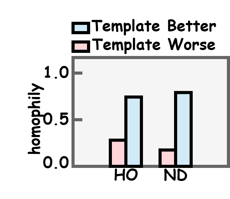
(a) Cora

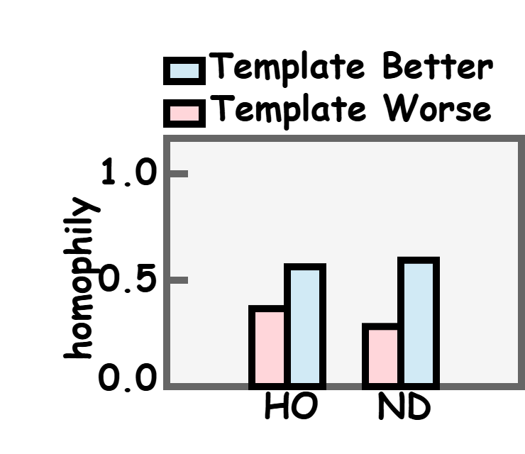
(b) PubMed

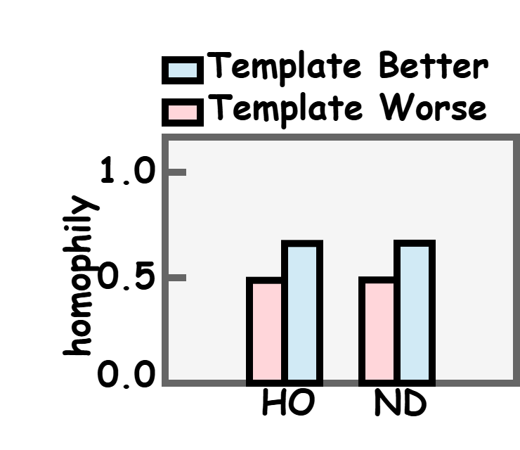
(c) Actor

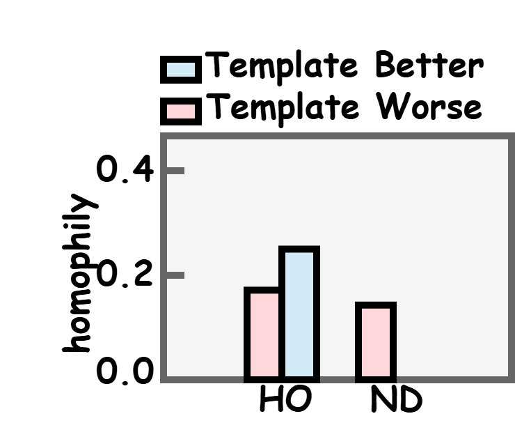
(d) Cornell

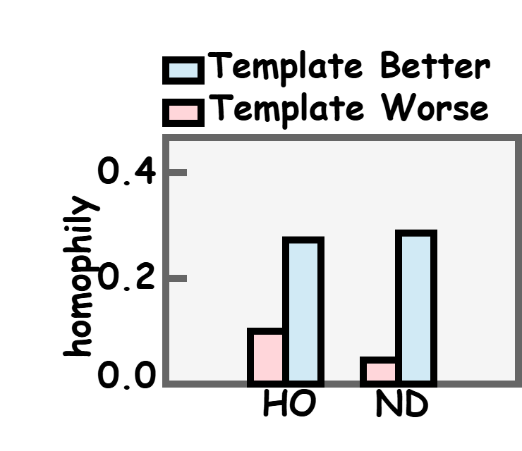
(e) Texas

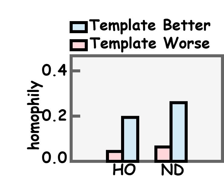
(f) Wisconsin

Figure 1: The average node-homophily for different types of nodes. "Template Better" means nodes which are predicted correctly by HO/ND but incorrectly by None, while "Template Worse" means nodes which are predicted incorrectly by HO/ND but correctly by None.

To further investigate this phenomenon, we examine the nodes where the predictions differ between different graph token lists. Specifically, we analyze two templates (HO and ND) and whether the performance is decreased or improved. We evaluate the node-homophily (proportion of 1-hop neighbors sharing the same label as the central node) of them. As shown in Figure 1, for all datasets, templates will be more likely to improve performance for nodes exhibit higher node-homophily. This further confirms that predefined templates are more beneficial for homophilic nodes but harmful for heterophilic nodes.

4.2 Theoretical Analysis

Next, we theoretically explore the graph token lists. We take HO as an example (the analysis of ND, which exhibits similar trends, is shown in Appendix E). Consider a graph with an average degree $n$. For a central node $u$, denote $\mathbf{T}_{u,0}^{\text{HO}}=\mathbf{x}_{u}$. The tokens are recursively calculated as $\mathbf{T}_{u,i}^{\text{HO}}=\frac{1}{n}\sum_{v\in\mathcal{N}_{u}}\mathbf{T}_{v,i-1}^{\text{HO}}$. To characterize nodes contributing to token $\mathbf{T}_{u,k}^{\text{HO}}$, we define $\mathbf{H}_{u}^{k}=\sum_{v\in\mathcal{N}_{u}^{k}}\mathbf{x}_{v}$ as the sum of the features of $\mathcal{N}_{u}^{k}$. $\mathbf{T}_{u,k}^{\text{HO}}$ can be expressed as a linear combination of $\mathbf{H}_{u}^{0},\dots,\mathbf{H}_{u}^{k}$, i.e.,

$$\mathbf{T}_{u,k}^{\text{HO}}=\sum\nolimits_{i=0}^{k}\mathbf{M}_{k,i}^{\text{HO}}\mathbf{H}_{u}^{i},$$ (2)

where $\mathbf{M}_{k,i}^{\text{HO}}$ is the matrix capturing the contribution of $\mathcal{N}_{u}^{i}$ to $\mathbf{T}_{u,k}^{\text{HO}}$. We can obtain $\mathbf{M}_{k,i}^{\text{HO}}$ as follows:

Theorem 4.1 (Recursive Properties of $\mathbf{M}_{k,i}^{\text{HO}}$).

$\mathbf{M}_{k,i}^{\text{HO}}$ follows the following rules:

1. $\mathbf{M}_{0,0}^{\text{HO}}=1$ ($\mathbf{T}_{u,0}^{\text{HO}}$ only contains the feature of node $u$);

2. $\mathbf{M}_{k,0}^{\text{HO}}=\mathbf{M}_{k-1,1}^{\text{HO}}$(contribution of $\mathcal{N}_{u}^{0}$ to $\mathbf{T}_{u,k}^{\text{HO}}$ equals that of $\mathcal{N}_{u}^{1}$ to $\mathbf{T}_{u,k-1}^{\text{HO}}$);

3. $\mathbf{M}_{k,i}^{\text{HO}}=\mathbf{0}$, $i>k$ (no contribution from higher-hop neighbors than the current hop depth);

4. $\mathbf{M}_{k,i}^{\text{HO}}=\frac{1}{n}\left(\mathbf{M}_{k-1,i-1}^{\text{HO}}+(n-1)\mathbf{M}_{k-1,i+1}^{\text{HO}}\right)$, for $k,i\geq 1$.

The proofs are shown in D.1. Building on Theorem 4.1, we derive the key properties and proofs of $\mathbf{M}_{k,i}^{\text{HO}}$ in Appendix D.2- D.4 that characterize the aggregation patterns of HO. These properties collectively reveal that HO contains an inherent bias of focusing more on near neighbors. For example, even within $\mathbf{T}_{u,k}^{\text{HO}}$, the far-hop neighbors (such as the $k$-th hop) are exponentially less influential than the near-hop ones as shown in Appendix D.4. Building on the properties of $\mathbf{M}_{i,k}^{\text{HO}}$, here we analyze how Tokenized Graph Learning Models interact with HO.

Theorem 4.2 (Effective Attention Allocation).

Consider a simplified 1-layer Transformer model processing $\mathbf{T}_{u,0}^{\text{HO}},\mathbf{T}_{u,1}^{\text{HO}},\dots,\mathbf{T}_{u,L}^{\text{HO}}$ for node $u$. Let $\alpha_{0},\alpha_{1},\dots,\alpha_{L}$ ($\sum_{i=0}^{L}\alpha_{i}=1$) denotes the attention scores from $\mathbf{T}_{u,0}^{\text{HO}}$ to all HO graph tokens. The effective attention allocated to $v\in\mathcal{N}_{u}^{k}$ is:

$$\hat{\alpha}_{k}=\sum\nolimits_{i=k,\,i\equiv k\,\text{mod}\,2}^{L}\alpha_{i}\mathbf{M}_{i,k}^{\text{HO}},$$ (3)

The allocation exhibits two critical properties: (1) Near-Hop Dominance: for $k_{1}<k_{2}$ with $k_{1}\equiv k_{2}\,\text{mod}\,2$, $\hat{\alpha}_{k_{1}}>\hat{\alpha}_{k_{2}}$. (2) Within-Hop Indistinguishability: for any $v_{1},v_{2}\in\mathcal{N}_{u}^{k}$, their effective attention scores satisfy: $\hat{\alpha}_{v_{1}}=\hat{\alpha}_{v_{2}}$.

The proof is given in Appendix D.5. Furthermore, to quantify how the hop-overpriority problem of HO impacts performance, we adopt the Frobenius norm of the difference between the raw node feature and its neighbors aggregated with attention as a metric (Shuman et al., 2013; Kalofolias, 2016), denoted as $\|\mathbf{H}_{u}^{0}-\hat{\mathbf{A}}\mathbf{H}^{0}\|_{F}$, where $\hat{\mathbf{A}}$ is the attention matrix derived from Theorem 4.2. Given the inherent bias of HO towards near-hop neighbors, we analyze how the hop-overpriority problem influences the metric:

Theorem 4.3 (Smoothness Bound of Tokenized Representations).

Let $C_{u}^{i}$ denote the proportion of $\mathcal{N}_{u}^{i}$ sharing the same label as node $u$. The smoothness of node $u$’s representation satisfies:

$$\|\mathbf{H}_{u}^{0}-\hat{\mathbf{A}}\mathbf{H}^{0}\|_{F}\leq\sqrt{2}L\sum\nolimits_{i=0}^{L}\hat{\alpha}_{i}|\mathcal{N}_{u}^{i}|(1-C_{u}^{i}),$$ (4)

where $L$ is a Lipschitz constant.

The proof is given in Appendix D.6. The bound clarifies how the hop-overpriority problem of HO interacts with graph homophily to influence the performance. On homophilic graphs, where $C_{u}^{i}$ is uniformly high even for near hops, the bound remains small, indicating the performance is not severely affected. However, heterophilic graphs exhibit low $C_{u}^{i}$ for odd hops, and $C_{u}^{i}$ increases with hop (i.e., $C_{u}^{i+2}>C_{u}^{i}$), but the effective attention $\hat{\alpha}_{i}$ decreases with hop. This leads to a critical mismatch: the hops with low $C_{u}^{i}$ receive high $\hat{\alpha}_{i}$, while hops with high $C_{u}^{i}$ are allocated low attention. Consequently, the bound grows significantly, limiting the ability of the models to learn meaningful representations, which aligns with our empirical results.

5 Method

In this section, we introduce our method in details. The overall framework is shown in Figure 2. LGTL s a simple-yet-effective plug-and-play module that can be easily compatible with various tokenized graph learning methods such as different variants of Graph LLMs and Graph Transformers.

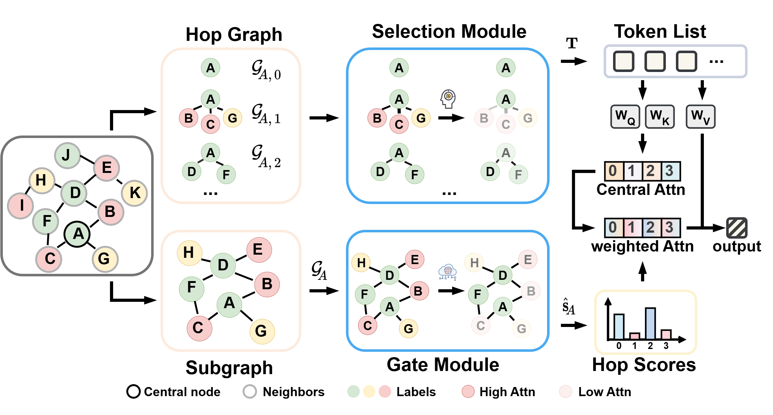
Figure 2: The overall framework of LGTL, including a gate module which learns hop scores from the central node’s subgraph to rebalance attention and mitigate hop-overpriority problem, and a selection module which constructs hop subgraphs, computes within-hop node attention, and aggregates features into tokens. These tokens form a list input to TGLMs; raw attention scores are adjusted by hop weights to produce task-adaptive representations for homophilic and heterophilic graphs.

5.1 LGTL: Learnable Token List for Tokenized Graph Learning Models

Inspired by our preliminary experiments and theoretical analysis, we propose LGTL, a learnable token list framework which flexibly adjusts the priority of hops and handles the features of nodes from different hops independently to focus on task-relevant signals. Specifically, LGTL adaptively allocates the attention in token lists by integrating the gate module and the selection module, enabling adaptive focus on task-relevant nodes across both homophilic and heterophilic datasets.

Given the total number of hops $L$ and the size of neighbor sampling $n_{i}$ (where $i\in\{1,2,\dots,L\}$), we adopt a gate module to flexibly assign scores to each hop. The gate module processes the subgraph $\mathcal{G}_{u}$ of the central node $u$ and learns context-aware embeddings leveraging a Graph Attention Network (GAT) (Veličković et al., 2018). To derive hop-specific weights, we first use the embedding of node $u$ from the gate module as raw scores $\mathbf{s}_{u}^{\text{raw}}\in\mathbb{R}^{L+1}$, which corresponds to the importance of different hops of neighbors. The scores are normalized through the softmax function to obtain the weights:

$$\hat{\mathbf{s}}_{u}=\text{Softmax}(\mathbf{s}_{u}^{\text{raw}}),$$ (5)

where $\hat{\mathbf{s}}_{u,i}$ denotes the weight assigned to the $i$-th hop. Intuitively, higher $\hat{\mathbf{s}}_{u,i}$ indicates the $i$-th hop is more important for the current tasks, which adaptively mitigates the hop-overpriority problem by re-balancing attention across the hops.

After obtaining the weights, we next construct the token list. For the $i$-th hop, LGTL constructs a hop token $\mathbf{T}_{i}$ by aggregating the features of the nodes in $\mathcal{N}_{u}^{i}$. Specifically, for the 0-th hop, the token is simply the raw feature of node, i.e., $\mathbf{T}_{0}=\mathbf{x}_{u}$. For the $i$-th hop ($i\geq 1$), LGTL samples $n_{i}$ nodes from $\mathcal{N}_{u}^{i}$, appends a self-loop edge, and forms a subgraph $\mathcal{G}_{u}^{i}$ with $n_{i}+1$ edges. A GAT layer is adopted as the selection module to process $\mathcal{G}_{u}^{i}$ and calculate the attention scores $\beta_{u,i,v}$ between $u$ and each $v$ sampled from $\mathcal{G}_{u}^{i}$. The $i$-th hop token is then obtained by weighted aggregation:

$$\mathbf{T}_{i}=\sum\nolimits_{v\in\mathcal{G}_{u}^{i}}\beta_{u,i,v}\cdot\mathbf{x}_{v},$$ (6)

where $\sum_{v\in\mathcal{G}_{u}^{i}}\beta_{u,i,v}=1$. Then, the token list $\mathbf{T}=[\mathbf{T}_{0},\mathbf{T}_{1},\dots,\mathbf{T}_{L}]$ is inputted into TGLMs to obtain the output of value matrix $\mathbf{T}\mathbf{W}_{V}$ and calculate the attention scores $\alpha_{u}=[\alpha_{u,0},\alpha_{u,1},\dots,\alpha_{u,L}]$ of the central node $u$, where $\alpha_{u,i}$ reflects the focus on the $i$-th hop token for node $u$. To align the attention with the scores we obtain from the gate module, LGTL adjusts $\alpha_{u}$ using $\hat{\mathbf{s}}_{u}$:

$$\hat{\alpha}_{u,i}=\frac{\alpha_{u,i}\cdot\hat{\mathbf{s}}_{u,i}}{\langle\alpha_{u}\cdot\hat{\mathbf{s}}_{u}\rangle},$$ (7)

where $\hat{\alpha}_{u,i}$ is the adjusted attention score for the $i$-th hop. The final node representation is obtained by aggregating the tokens with the adjusted scores:

$$\mathbf{z}_{u}=\sum\nolimits_{i=0}^{L}\hat{\alpha}_{u,i}\cdot\mathbf{T}_{i}\mathbf{W}_{V},$$ (8)

In sum, by adaptively weighting hops via $\hat{\mathbf{s}}_{u}$ and refining the aggregation process of features via the selection module, LGTL adapts to homophilic and heterophilic graphs, ensuring that the task-relevant nodes hold a leading position of the aggregation process.

5.2 Theoreical Analysis

To verify the design of LGTL, we present theoretical properties that explain its adaptability and generality over predefined token lists. A key strength of LGTL is its flexibility to accommodate various tokenization strategies by adjusting its learnable components. Specifically, LGTL can recover the behavior of existing predefined templates (e.g., HO and ND) through parameter specialization, highlighting its ability to generalize prior approaches. We formalize the following theorem:

Theorem 5.1.

LGTL generalizes pre-defined token lists HO and ND as special cases.

Proof.

For HO, the attention to $k$-th hop nodes is $\hat{\alpha}_{k}=\sum_{i=k,\,i\equiv k\,\text{mod}\,2}^{L}\alpha_{i}\mathbf{M}_{i,k}^{\text{HO}}$, where $\mathbf{M}_{i,k}^{\text{HO}}$ is the hop contribution matrix. For LGTL, setting $\mathcal{G}_{u}^{i}=\mathcal{N}_{u}^{i}$, $\beta_{u,k,v}=\frac{1}{|\mathcal{N}_{u}^{k}|}$ ,and $\hat{\alpha}_{u,k}=\frac{\hat{\alpha}_{k}}{\beta_{u,k,v}}$ leads to

$$s_{u,k}\propto\frac{\hat{\alpha}_{k}}{\beta_{u,k,v}\cdot\alpha_{u,i}},$$ (9)

This can recover the attention of HO. Thus, HO is a special case of LGTL with uniform within-hop attention and fixed gate weights. The proof of ND is provided in Appendix F.2.∎

Furthermore, to quantitatively analyze how our method tackles the hop-overpriority problem, we re-examine the bound in Theorem 4.3.

Theorem 5.2.

The norm of LGTL is bounded by:

$$\|\mathbf{H}_{u}^{0}-\hat{\mathbf{A}}\mathbf{H}^{0}\|_{F}\leq\sqrt{2}L\cdot\frac{\sum_{i=0}^{L}\hat{\mathbf{s}}_{u,i}|\mathcal{G}_{u}^{i}|(1-C_{u}^{i})}{\sum_{i=0}^{L}|\mathcal{G}_{u}^{i}|(1-C_{u}^{i})+\frac{\eta_{u}}{\gamma_{u}}\sum_{i=0}^{L}|\mathcal{G}_{u}^{i}|C_{u}^{i}},$$ (10)

where $\gamma_{u}=\mathbb{E}_{v\in\mathbf{N}_{u}^{i},\mathbf{y}_{u}=\mathbf{y}_{v}}\exp\left(\frac{\mathbf{q}_{u}\mathbf{k}_{v}^{\top}}{\sqrt{h}}\right)$, and $\eta_{u}=\mathbb{E}_{v\in\mathbf{N}_{u}^{i},\mathbf{y}_{u}\neq\mathbf{y}_{v}}\exp\left(\frac{\mathbf{q}_{u}\mathbf{k}_{v}^{\top}}{\sqrt{h}}\right)$ are constants.

Detailed analysis and proofs are in Appendix F.3. This theorem shows that LGTL minimizes the error by assigning higher $\hat{\mathbf{s}}_{u,i}$ to hops with higher $C_{u}^{i}$, which is critical for heterophilic graphs, where predefined token lists pay more attention to inconsistent hops according to Theorem 4.3.

6 Experiments

In this section, we conduct experiments to answer the following research questions. Q1: Is LGTL capable of augmenting existing LLMs for graphs for text-attributed graphs? Q2: Is LGTL effective in enhancing graph Transformers without texts? Q3: How does each component contribute to LGTL?

6.1 Results on Text-attributed Graphs

To answer Q1, we first conduct experiments on text-attributed graphs.

Experimental Setups: we choose LLaGA Chen et al. (2024a), a representative Graph LLM, as our backbone. Specifically, we replace the token list of LLaGA with LGTL and keep other parts unchanged. Besides comparing LLaGA with different token lists, i.e., HO/HD, we also compare LGTL with four additional baselines, including two classical GNNs, GCN (Kipf and Welling, 2017) and GAT (Veličković et al., 2018), and one GNN for heterophilic graphs, H2GCN (Zhu et al., 2020), and one representative Graph Transformer, NodeFormer (wu2022NodeFormer). For datasets, we follow (Chen et al., 2024a) and use two homophilic datasets, Cora and PubMed. For heterophilic datasets, we use Cornell, Texas, Wisconsin, and Actor by collecting the texts of all nodes and relations between them. More details are provided in Appendix A.1.

Results: Table 2 presents the results for text-attributed graphs. LLaGA-LGTL consistently outperforms both classical GNNs and LLaGA variants with original token lists across node classification and link prediction tasks. For node classification, LLaGA-LGTL achieves the best accuracy on all six datasets, with an average improvement of 10.39% over LLaGA-HO and LLaGA-ND. In particular, its superiority is more pronounced on heterophilic datasets. For link prediction, LLaGA-LGTL also leads, achieving an average gain of  4.67% over the second-best baseline across all six datasets. This consistent improvement underscores its capability to better align attention with task-relevant edges.

Table 2: The results on six text-attributed graphs with LLaGA as the backbone, where bold signifies the best result and underline highlights the second best result.

Task	Model	Cora	PubMed	Cornell	Texas	Wisconsin	Actor
Node Classification	GCN	88.93 ±0.12	92.96 ±0.15	40.00 ±3.12	56.13 ±2.89	45.83 ±3.15	70.57 ±0.34
	GAT	88.97 ±0.14	92.33 ±0.18	36.67 ±4.13	56.77 ±2.24	43.75 ±3.60	69.11 ±0.36
	H2GCN	88.82 ±0.11	93.61 ±0.13	58.67 ±2.28	82.58 ±0.79	69.58 ±1.95	74.62 ±0.40
	NodeFormer	88.23 ±0.17	94.90 ±0.19	55.33 ±3.34	81.29 ±1.25	65.83 ±2.62	76.23 ±0.42
	LLaGA-HO	89.22 ±0.10	95.03 ±0.12	42.67 ±4.38	63.23 ±2.97	49.58 ±3.74	77.05 ±0.41
	LLaGA-ND	88.86 ±0.13	95.03 ±0.14	46.67 ±4.38	74.19 ±1.91	50.83 ±3.60	77.34 ±0.39
	LLaGA-LGTL	89.30 ±0.09	95.18 ±0.11	64.67 ±1.21	90.32 ±0.68	77.08 ±0.79	79.04 ±0.37
Link Prediction	GCN	81.24 ±0.21	90.50 ±0.23	66.52 ±2.29	74.00 ±1.78	71.49 ±1.57	74.55 ±0.44
	GAT	79.68 ±0.23	88.67 ±0.25	65.22 ±2.36	69.20 ±1.86	73.26 ±1.65	74.82 ±0.46
	H2GCN	80.24 ±0.20	88.03 ±0.22	70.43 ±1.32	72.80 ±1.81	72.56 ±1.60	75.12 ±0.45
	NodeFormer	78.12 ±0.24	79.38 ±0.26	57.83 ±2.40	64.40 ±1.93	68.14 ±1.71	64.62 ±0.47
	LLaGA-HO	81.17 ±0.19	89.72 ±0.21	62.17 ±1.39	71.40 ±1.92	65.00 ±1.70	86.23 ±0.42
	LLaGA-ND	82.29 ±0.18	91.31 ±0.20	63.04 ±1.35	71.60 ±1.89	64.44 ±1.67	86.44 ±0.41
	LLaGA-LGTL	83.82 ±0.16	91.84 ±0.18	71.30 ±0.74	76.80 ±0.72	73.95 ±0.93	89.48 ±0.38

6.2 Results on Benchmarks for Graph Transformers

To answer Q2, we further conduct experiments on benchmarks without text for Graph Transformers.

Experimental Setups: we choose two classical Graph Transformers for evaluation: NAGphormer (Chen et al., 2022a), and VCR-Graphormer (Fu et al., 2024). Similar to Graph LLMs, we replace the token list of NAGphormer and VCR-Graphormer with LGTL and keep other parts unchanged. Other baselines are the same as Section 6.1. For datasets, we follow NAGphormer and VCR-Graphormer by using PubMed (Namata et al., 2012), Computers, and Photo (Shchur et al., 2018) with numerical node features. Additionally, we adopt four heterophilic datasets (Cornell, Texas, Wisconsin, and Actor (Pei et al., 2020)). More details are provided in Appendix A.2.

Table 3: The results on seven graph benchmark datasets without using text with NAGphormer and VCR-Graphormer as the backbone, where bold signifies the best result.

Model	PubMed	Computers	Photo	Cornell	Texas	Wisconsin	Actor
GCN	86.54 ±0.21	89.65 ±0.24	92.70 ±0.27	47.37 ±3.25	52.63 ±2.74	54.09 ±2.52	29.87 ±1.03
GAT	86.32 ±0.23	90.78 ±0.26	93.87 ±0.29	44.74 ±4.31	55.26 ±2.82	52.94 ±3.60	29.08 ±1.41
H2GCN	88.49 ±0.19	89.86 ±0.22	94.95 ±0.25	63.16 ±2.28	65.79 ±1.79	66.67 ±1.55	34.74 ±0.69
NodeFormer	88.89 ±0.20	90.96 ±0.23	95.02 ±0.26	60.53 ±2.34	65.79 ±1.85	62.75 ±2.62	34.87 ±0.80
NAGphormer	89.55 ±0.18	91.22 ±0.21	95.49 ±0.24	55.26 ±1.38	63.16 ±1.91	62.75 ±1.68	34.61 ±0.67
NAGphormer-LGTL	90.11 ±0.10	91.78 ±0.12	96.01 ±0.15	65.79 ±1.21	73.68 ±1.68	81.57 ±1.49	36.84 ±0.51
VCR-Graphormer	88.82 ±0.17	90.51 ±0.20	95.53 ±0.23	52.63 ±1.29	65.79 ±1.78	60.78 ±1.57	35.59 ±0.36
VCR-Graphormer-LGTL	89.45 ±0.12	91.13 ±0.14	95.82 ±0.17	68.42 ±1.24	73.68 ±1.72	79.22 ±1.53	38.03 ±0.42

Results: The results on benchmarks for Graph Transformers are shown in Table 3. When integrating LGTL into NAGphormer and VCR-Graphormer, both models exhibit significant improvements over their original versions and classical baselines. For instance, NAGphormer-LGTL outperforms the original NAGphormer by 0.55% average on homophilic datasets, while achieving 10.53% average on heterophilic datasets. Similarly, VCR-Graphormer-LGTL shows a 11.14% average improvement on heterophilic datasets, with top performance on all seven benchmarks. These results confirm the effectiveness of LGTL in enhancing TGLMs, particularly under heterophily, aligning with our analysis of the hop-overpriority problem.

6.3 Ablation Studies & Analysis

To answer Q3, next we conduct ablation studies and detailed analyses for each component.

Ablation Studies. First, we carry out ablation studies to evaluate the gate module and the selection module of LGTL. Specifically, we compare two variants: “w/o gate” denotes removing the gate module by setting same weights for all hops. “w/o selection” indicates removing the selection module by letting the neighbors of the central node share the same attention score. The results are shown in Table 4. We can observe that: (1) “w/o gate” underperforms LGTL on all datasets, demonstrating its effectiveness in focusing on task-relevant hops; (2) “w/o selection” also lags behind LGTL, indicating the effectiveness of the selection module in distinguishing critical within-hop nodes; (3) the performance decrease is more severe on heterophilic datasets, indicating the indispensable role of hop-level (gate) and within-hop (selection) mechanisms in adapting to heterophilic graphs.

Table 4: The results of ablation studies for the gate and selection module of LGTL.

Model	LLaGA Cora	LLaGA Texas	NAG PubMed	NAG Actor	VCR PubMed	VCR Actor
w/o gate	89.14	80.65	89.40	35.66	89.02	36.83
w/o selection	89.11	70.97	89.58	35.07	88.89	35.99
LGTL(full)	89.30	90.32	90.11	36.84	89.45	38.03

Analysis of the gate module. Next, we analyze the scores the gate module assigns to different hops for a more fine-grained analysis. Intuitively, hops with higher node-homophily indicate nodes with the same label and thus the gate module should allocate higher attention scores. As shown in Figure 3, on homophilic graphs, the gate module allocates the highest scores to “hop 1”, followed by “hop 2”, while on heterophilic graphs, the gate module instead focuses more on “hop 2” and the central node. The results indicate that the gate module assign larger weights to hops with higher task-relevance.

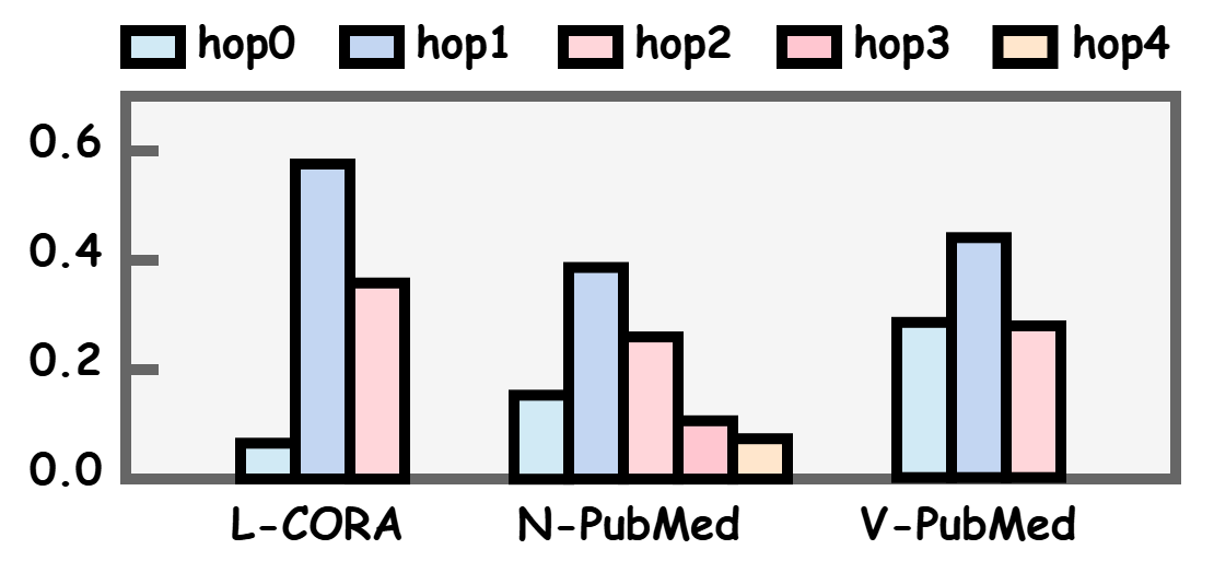
(a) Homophilic Graphs

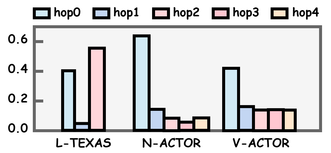
(b) Heterophilic Graphs

Figure 3: The analysis of the score by the gate module vs. the number of hops. “L”, “N”, and “V” indicates abbreviation for LLaGA, NAGphormer, and VCR-Graphormer, respectively.

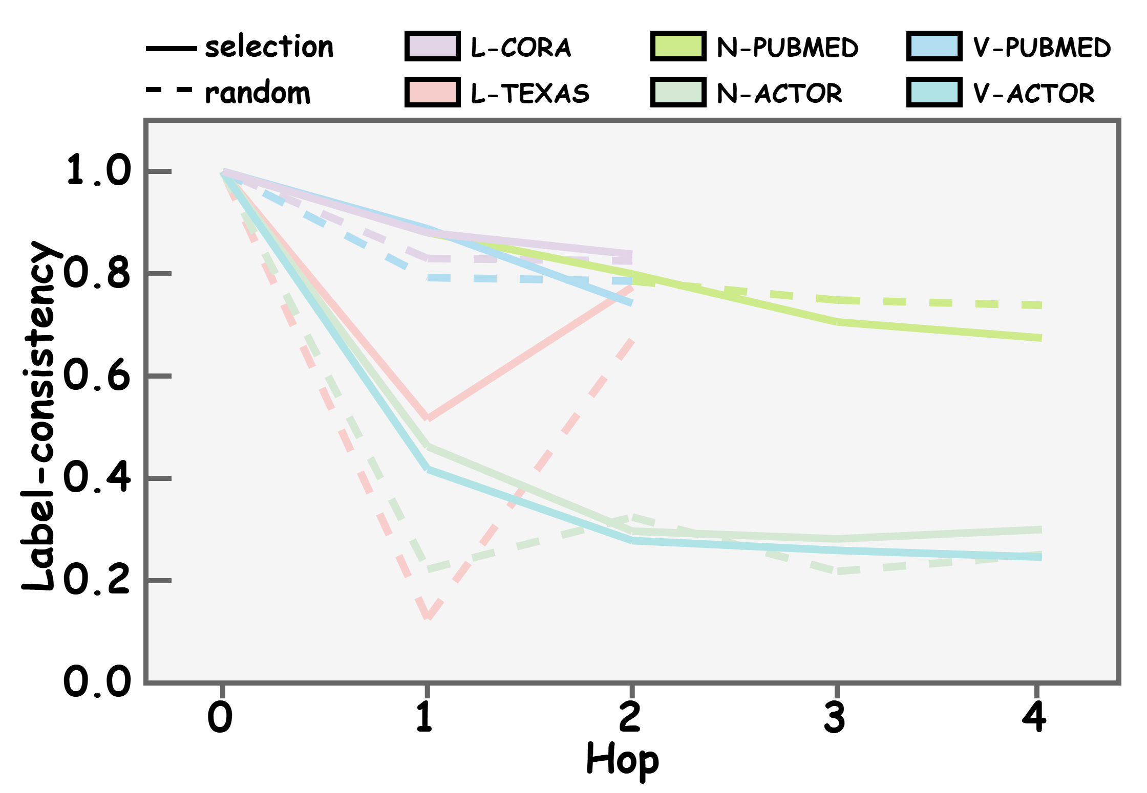
Figure 4: The label-consistency of the selection module and node-homophily of hops. “L”, “N”, and “V” indicates abbreviation for LLaGA, NAGphormer, and VCR-Graphormer, respectively.

Analysis of the selection module. Lastly, we aim to analyze whether the selection module can select nodes with the same label as the central nodes. Therefore, we analyze the label-consistency of nodes with the highest attention scores within each hop. As a reference line, we compare with randomly selecting nodes from each hop. As shown in Figure 4, the label-consistency of the selected nodes exceeds the random baseline, indicating that the selection module effectively identifies and prioritizes critical nodes. We provide more experiments and analysis of LGTL in Appendix B.

7 Conclusion

In this paper, we first identify the hop-overpriority problem for predefined token lists in TGLMs.Then, we propose Learnable Graph Token List (LGTL), an adaptive framework that adjusts hop weights and prioritizes informative nodes within and across hops, enhancing the adaptability on both homophilic and heterophilic graphs. We also theoretically show that LGTL can effective address the hop-overpriority problem. Experiments across diverse TGLM backbones demonstrate that LGTL consistently improves performance and mitigate the hop-overpriority problem.

NeurIPS Paper Checklist

The checklist is designed to encourage best practices for responsible machine learning research, addressing issues of reproducibility, transparency, research ethics, and societal impact. Do not remove the checklist: The papers not including the checklist will be desk rejected. The checklist should follow the references and follow the (optional) supplemental material. The checklist does NOT count towards the page limit.

Please read the checklist guidelines carefully for information on how to answer these questions. For each question in the checklist:

• You should answer [Yes] , [No] , or [N/A] .

• [N/A] means either that the question is Not Applicable for that particular paper or the relevant information is Not Available.

• Please provide a short (1–2 sentence) justification right after your answer (even for NA).

The checklist answers are an integral part of your paper submission. They are visible to the reviewers, area chairs, senior area chairs, and ethics reviewers. You will be asked to also include it (after eventual revisions) with the final version of your paper, and its final version will be published with the paper.

The reviewers of your paper will be asked to use the checklist as one of the factors in their evaluation. While "[Yes] " is generally preferable to "[No] ", it is perfectly acceptable to answer "[No] " provided a proper justification is given (e.g., "error bars are not reported because it would be too computationally expensive" or "we were unable to find the license for the dataset we used"). In general, answering "[No] " or "[N/A] " is not grounds for rejection. While the questions are phrased in a binary way, we acknowledge that the true answer is often more nuanced, so please just use your best judgment and write a justification to elaborate. All supporting evidence can appear either in the main paper or the supplemental material, provided in appendix. If you answer [Yes] to a question, in the justification please point to the section(s) where related material for the question can be found.

1. Claims

2. Question: Do the main claims made in the abstract and introduction accurately reflect the paper’s contributions and scope?

3. Answer: [Yes]

4. Justification: The abstract and introduction accurately reflect the paper’s contributions and scope.

5. Guidelines:

   • The answer NA means that the abstract and introduction do not include the claims made in the paper.

   • The abstract and/or introduction should clearly state the claims made, including the contributions made in the paper and important assumptions and limitations. A No or NA answer to this question will not be perceived well by the reviewers.

   • The claims made should match theoretical and experimental results, and reflect how much the results can be expected to generalize to other settings.

   • It is fine to include aspirational goals as motivation as long as it is clear that these goals are not attained by the paper.

6. Limitations

7. Question: Does the paper discuss the limitations of the work performed by the authors?

8. Answer: [Yes]

9. Justification: We provide detailed discussions about limitations in Appendix C.1.

10. Guidelines:

    • The answer NA means that the paper has no limitation while the answer No means that the paper has limitations, but those are not discussed in the paper.

    • The authors are encouraged to create a separate "Limitations" section in their paper.

    • The paper should point out any strong assumptions and how robust the results are to violations of these assumptions (e.g., independence assumptions, noiseless settings, model well-specification, asymptotic approximations only holding locally). The authors should reflect on how these assumptions might be violated in practice and what the implications would be.

    • The authors should reflect on the scope of the claims made, e.g., if the approach was only tested on a few datasets or with a few runs. In general, empirical results often depend on implicit assumptions, which should be articulated.

    • The authors should reflect on the factors that influence the performance of the approach. For example, a facial recognition algorithm may perform poorly when image resolution is low or images are taken in low lighting. Or a speech-to-text system might not be used reliably to provide closed captions for online lectures because it fails to handle technical jargon.

    • The authors should discuss the computational efficiency of the proposed algorithms and how they scale with dataset size.

    • If applicable, the authors should discuss possible limitations of their approach to address problems of privacy and fairness.

    • While the authors might fear that complete honesty about limitations might be used by reviewers as grounds for rejection, a worse outcome might be that reviewers discover limitations that aren’t acknowledged in the paper. The authors should use their best judgment and recognize that individual actions in favor of transparency play an important role in developing norms that preserve the integrity of the community. Reviewers will be specifically instructed to not penalize honesty concerning limitations.

11. Theory assumptions and proofs

12. Question: For each theoretical result, does the paper provide the full set of assumptions and a complete (and correct) proof?

13. Answer: [Yes]

14. Justification: We provide complete theory assumptions and proofs of pre-defined token list in Appendix D and Appendix E. Furthermore, we provide the theory assumptions and proofs of LGTL in Appendix F.

15. Guidelines:

    • The answer NA means that the paper does not include theoretical results.

    • All the theorems, formulas, and proofs in the paper should be numbered and cross-referenced.

    • All assumptions should be clearly stated or referenced in the statement of any theorems.

    • The proofs can either appear in the main paper or the supplemental material, but if they appear in the supplemental material, the authors are encouraged to provide a short proof sketch to provide intuition.

    • Inversely, any informal proof provided in the core of the paper should be complemented by formal proofs provided in appendix or supplemental material.

    • Theorems and Lemmas that the proof relies upon should be properly referenced.

16. Experimental result reproducibility

17. Question: Does the paper fully disclose all the information needed to reproduce the main experimental results of the paper to the extent that it affects the main claims and/or conclusions of the paper (regardless of whether the code and data are provided or not)?

18. Answer: [Yes]

19. Justification: Yes, we disclose all the information needed to reproduce the main experimental results of the paper in Appendix A.3.

20. Guidelines:

    • The answer NA means that the paper does not include experiments.

    • If the paper includes experiments, a No answer to this question will not be perceived well by the reviewers: Making the paper reproducible is important, regardless of whether the code and data are provided or not.

    • If the contribution is a dataset and/or model, the authors should describe the steps taken to make their results reproducible or verifiable.

    • Depending on the contribution, reproducibility can be accomplished in various ways. For example, if the contribution is a novel architecture, describing the architecture fully might suffice, or if the contribution is a specific model and empirical evaluation, it may be necessary to either make it possible for others to replicate the model with the same dataset, or provide access to the model. In general. releasing code and data is often one good way to accomplish this, but reproducibility can also be provided via detailed instructions for how to replicate the results, access to a hosted model (e.g., in the case of a large language model), releasing of a model checkpoint, or other means that are appropriate to the research performed.

    • While NeurIPS does not require releasing code, the conference does require all submissions to provide some reasonable avenue for reproducibility, which may depend on the nature of the contribution. For example

      1. If the contribution is primarily a new algorithm, the paper should make it clear how to reproduce that algorithm.

      2. If the contribution is primarily a new model architecture, the paper should describe the architecture clearly and fully.

      3. If the contribution is a new model (e.g., a large language model), then there should either be a way to access this model for reproducing the results or a way to reproduce the model (e.g., with an open-source dataset or instructions for how to construct the dataset).

      4. We recognize that reproducibility may be tricky in some cases, in which case authors are welcome to describe the particular way they provide for reproducibility. In the case of closed-source models, it may be that access to the model is limited in some way (e.g., to registered users), but it should be possible for other researchers to have some path to reproducing or verifying the results.

21. Open access to data and code

22. Question: Does the paper provide open access to the data and code, with sufficient instructions to faithfully reproduce the main experimental results, as described in supplemental material?

23. Answer: [Yes]

24. Justification: Yes, we provide our code in the supplemental material.

25. Guidelines:

    • The answer NA means that paper does not include experiments requiring code.

    • Please see the NeurIPS code and data submission guidelines (https://nips.cc/public/guides/CodeSubmissionPolicy) for more details.

    • While we encourage the release of code and data, we understand that this might not be possible, so “No” is an acceptable answer. Papers cannot be rejected simply for not including code, unless this is central to the contribution (e.g., for a new open-source benchmark).

    • The instructions should contain the exact command and environment needed to run to reproduce the results. See the NeurIPS code and data submission guidelines (https://nips.cc/public/guides/CodeSubmissionPolicy) for more details.

    • The authors should provide instructions on data access and preparation, including how to access the raw data, preprocessed data, intermediate data, and generated data, etc.

    • The authors should provide scripts to reproduce all experimental results for the new proposed method and baselines. If only a subset of experiments are reproducible, they should state which ones are omitted from the script and why.

    • At submission time, to preserve anonymity, the authors should release anonymized versions (if applicable).

    • Providing as much information as possible in supplemental material (appended to the paper) is recommended, but including URLs to data and code is permitted.

26. Experimental setting/details

27. Question: Does the paper specify all the training and test details (e.g., data splits, hyperparameters, how they were chosen, type of optimizer, etc.) necessary to understand the results?

28. Answer: [Yes]

29. Justification: Yes, all the training and test details are provided in Section 6 and Appendix A.

30. Guidelines:

    • The answer NA means that the paper does not include experiments.

    • The experimental setting should be presented in the core of the paper to a level of detail that is necessary to appreciate the results and make sense of them.

    • The full details can be provided either with the code, in appendix, or as supplemental material.

31. Experiment statistical significance

32. Question: Does the paper report error bars suitably and correctly defined or other appropriate information about the statistical significance of the experiments?

33. Answer: [Yes]

34. Justification: Yes, our main experimental results in Table 2 and Table 3 report error bars.

35. Guidelines:

    • The answer NA means that the paper does not include experiments.

    • The authors should answer "Yes" if the results are accompanied by error bars, confidence intervals, or statistical significance tests, at least for the experiments that support the main claims of the paper.

    • The factors of variability that the error bars are capturing should be clearly stated (for example, train/test split, initialization, random drawing of some parameter, or overall run with given experimental conditions).

    • The method for calculating the error bars should be explained (closed form formula, call to a library function, bootstrap, etc.)

    • The assumptions made should be given (e.g., Normally distributed errors).

    • It should be clear whether the error bar is the standard deviation or the standard error of the mean.

    • It is OK to report 1-sigma error bars, but one should state it. The authors should preferably report a 2-sigma error bar than state that they have a 96% CI, if the hypothesis of Normality of errors is not verified.

    • For asymmetric distributions, the authors should be careful not to show in tables or figures symmetric error bars that would yield results that are out of range (e.g. negative error rates).

    • If error bars are reported in tables or plots, The authors should explain in the text how they were calculated and reference the corresponding figures or tables in the text.

36. Experiments compute resources

37. Question: For each experiment, does the paper provide sufficient information on the computer resources (type of compute workers, memory, time of execution) needed to reproduce the experiments?

38. Answer: [Yes]

39. Justification: Sufficient information on the computer resources is provided in Appendix A.3.

40. Guidelines:

    • The answer NA means that the paper does not include experiments.

    • The paper should indicate the type of compute workers CPU or GPU, internal cluster, or cloud provider, including relevant memory and storage.

    • The paper should provide the amount of compute required for each of the individual experimental runs as well as estimate the total compute.

    • The paper should disclose whether the full research project required more compute than the experiments reported in the paper (e.g., preliminary or failed experiments that didn’t make it into the paper).

41. Code of ethics

42. Question: Does the research conducted in the paper conform, in every respect, with the NeurIPS Code of Ethics https://neurips.cc/public/EthicsGuidelines?

43. Answer: [Yes]

44. Justification: Yes, we have read the NeurIPS Code of Ethics and our paper conforms, in every respect, with the NeurIPS Code of Ethics.

45. Guidelines:

    • The answer NA means that the authors have not reviewed the NeurIPS Code of Ethics.

    • If the authors answer No, they should explain the special circumstances that require a deviation from the Code of Ethics.

    • The authors should make sure to preserve anonymity (e.g., if there is a special consideration due to laws or regulations in their jurisdiction).

46. Broader impacts

47. Question: Does the paper discuss both potential positive societal impacts and negative societal impacts of the work performed?

48. Answer: [Yes]

49. Justification: We discuss both potential positive societal impacts and negative societal impacts of the work in Appendix C.2.

50. Guidelines:

    • The answer NA means that there is no societal impact of the work performed.

    • If the authors answer NA or No, they should explain why their work has no societal impact or why the paper does not address societal impact.

    • Examples of negative societal impacts include potential malicious or unintended uses (e.g., disinformation, generating fake profiles, surveillance), fairness considerations (e.g., deployment of technologies that could make decisions that unfairly impact specific groups), privacy considerations, and security considerations.

    • The conference expects that many papers will be foundational research and not tied to particular applications, let alone deployments. However, if there is a direct path to any negative applications, the authors should point it out. For example, it is legitimate to point out that an improvement in the quality of generative models could be used to generate deepfakes for disinformation. On the other hand, it is not needed to point out that a generic algorithm for optimizing neural networks could enable people to train models that generate Deepfakes faster.

    • The authors should consider possible harms that could arise when the technology is being used as intended and functioning correctly, harms that could arise when the technology is being used as intended but gives incorrect results, and harms following from (intentional or unintentional) misuse of the technology.

    • If there are negative societal impacts, the authors could also discuss possible mitigation strategies (e.g., gated release of models, providing defenses in addition to attacks, mechanisms for monitoring misuse, mechanisms to monitor how a system learns from feedback over time, improving the efficiency and accessibility of ML).

51. Safeguards

52. Question: Does the paper describe safeguards that have been put in place for responsible release of data or models that have a high risk for misuse (e.g., pretrained language models, image generators, or scraped datasets)?

53. Answer: [N/A]

54. Justification: The paper poses no such risks.

55. Guidelines:

    • The answer NA means that the paper poses no such risks.

    • Released models that have a high risk for misuse or dual-use should be released with necessary safeguards to allow for controlled use of the model, for example by requiring that users adhere to usage guidelines or restrictions to access the model or implementing safety filters.

    • Datasets that have been scraped from the Internet could pose safety risks. The authors should describe how they avoided releasing unsafe images.

    • We recognize that providing effective safeguards is challenging, and many papers do not require this, but we encourage authors to take this into account and make a best faith effort.

56. Licenses for existing assets

57. Question: Are the creators or original owners of assets (e.g., code, data, models), used in the paper, properly credited and are the license and terms of use explicitly mentioned and properly respected?

58. Answer: [Yes]

59. Justification: We have cited the original paper that produced the code package or dataset.

60. Guidelines:

    • The answer NA means that the paper does not use existing assets.

    • The authors should cite the original paper that produced the code package or dataset.

    • The authors should state which version of the asset is used and, if possible, include a URL.

    • The name of the license (e.g., CC-BY 4.0) should be included for each asset.

    • For scraped data from a particular source (e.g., website), the copyright and terms of service of that source should be provided.

    • If assets are released, the license, copyright information, and terms of use in the package should be provided. For popular datasets, paperswithcode.com/datasets has curated licenses for some datasets. Their licensing guide can help determine the license of a dataset.

    • For existing datasets that are re-packaged, both the original license and the license of the derived asset (if it has changed) should be provided.

    • If this information is not available online, the authors are encouraged to reach out to the asset’s creators.

61. New assets

62. Question: Are new assets introduced in the paper well documented and is the documentation provided alongside the assets?

63. Answer: [N/A]

64. Justification: The paper does not release new assets.

65. Guidelines:

    • The answer NA means that the paper does not release new assets.

    • Researchers should communicate the details of the dataset/code/model as part of their submissions via structured templates. This includes details about training, license, limitations, etc.

    • The paper should discuss whether and how consent was obtained from people whose asset is used.

    • At submission time, remember to anonymize your assets (if applicable). You can either create an anonymized URL or include an anonymized zip file.

66. Crowdsourcing and research with human subjects

67. Question: For crowdsourcing experiments and research with human subjects, does the paper include the full text of instructions given to participants and screenshots, if applicable, as well as details about compensation (if any)?

68. Answer: [N/A]

69. Justification: The paper does not involve crowdsourcing nor research with human subjects.

70. Guidelines:

    • The answer NA means that the paper does not involve crowdsourcing nor research with human subjects.

    • Including this information in the supplemental material is fine, but if the main contribution of the paper involves human subjects, then as much detail as possible should be included in the main paper.

    • According to the NeurIPS Code of Ethics, workers involved in data collection, curation, or other labor should be paid at least the minimum wage in the country of the data collector.

71. Institutional review board (IRB) approvals or equivalent for research with human subjects

72. Question: Does the paper describe potential risks incurred by study participants, whether such risks were disclosed to the subjects, and whether Institutional Review Board (IRB) approvals (or an equivalent approval/review based on the requirements of your country or institution) were obtained?

73. Answer: [N/A]

74. Justification: The paper does not involve crowdsourcing nor research with human subjects.

75. Guidelines:

    • The answer NA means that the paper does not involve crowdsourcing nor research with human subjects.

    • Depending on the country in which research is conducted, IRB approval (or equivalent) may be required for any human subjects research. If you obtained IRB approval, you should clearly state this in the paper.

    • We recognize that the procedures for this may vary significantly between institutions and locations, and we expect authors to adhere to the NeurIPS Code of Ethics and the guidelines for their institution.

    • For initial submissions, do not include any information that would break anonymity (if applicable), such as the institution conducting the review.

76. Declaration of LLM usage

77. Question: Does the paper describe the usage of LLMs if it is an important, original, or non-standard component of the core methods in this research? Note that if the LLM is used only for writing, editing, or formatting purposes and does not impact the core methodology, scientific rigorousness, or originality of the research, declaration is not required.

78. Answer: [N/A]

79. Justification: The paper does not use LLMs as an important, original, or non-standard component.

80. Guidelines:

    • The answer NA means that the core method development in this research does not involve LLMs as any important, original, or non-standard components.

    • Please refer to our LLM policy (https://neurips.cc/Conferences/2025/LLM) for what should or should not be described.

Appendix A Details of Datasets and Environment

A.1 Datasets in LLaGA

Table 5: Dataset Statistics

Datasets	# Nodes	# Edges	# Classes	# Features	# homophily	Split ratio
Cora	2,708	10,556	7	2,432	0.83	60%/20%/20%
PubMed	19,717	88,648	3	2,432	0.79	60%/20%/20%
Cornell	151	456	5	2,432	0.13	60%/20%/20%
Texas	156	496	5	2,432	0.13	60%/20%/20%
Wisconsin	244	846	5	2,432	0.18	60%/20%/20%
Actor	9,228	272,862	5	2,432	0.67	60%/20%/20%

Cornell, Texas, and Wisconsin: https://www.cs.cmu.edu/afs/cs.cmu.edu/project/theo-20/www/data/
For Actor, we get the raw texts of 5 classes from:

• American_film_actors: https://en.wikipedia.org/wiki/Category:American_film_actors

• American_television_actors: https://en.wikipedia.org/wiki/Category:American_television_actors

• American_screenwriters: https://en.wikipedia.org/wiki/Category:American_screenwriters

• American_stage_actors: https://en.wikipedia.org/wiki/Category:American_stage_actors

• American_film_directors: https://en.wikipedia.org/wiki/Category:American_film_directors

A.2 Datasets in NAGphormer and VCR-Graphormer

Table 6: Dataset Statistics

Datasets	# Nodes	# Edges	# Classes	# Features	# homophily	Split ratio
PubMed	19,717	88,651	3	500	0.79	60%/20%/20%
Computers	13,752	441,512	10	767	0.70	60%/20%/20%
Photo	7,650	223,538	8	745	0.77	60%/20%/20%
Cornell	183	590	5	1,703	0.11	60%/20%/20%
Texas	183	618	5	1,703	0.06	60%/20%/20%
Wisconsin	251	998	5	1,703	0.16	60%/20%/20%
Actor	7,600	33,544	5	931	0.24	60%/20%/20%

All of these datasets can be accessed from the DGL library.

A.3 Environment

The environment where our codes run is as follows:

• OS: Linux 5.4.0-131-generic

• CPU: Intel(R) Xeon(R) Gold 6348 CPU @ 2.60GHz

• GPU: GeForce RTX 3090

Appendix B More Experiments and Analysis on LGTL

B.1 Attention Scores Allocated to Hops

To further validate the effectiveness of LGTL, we analyze the actual attention scores assigned to each hop by LGTL and HO, calculated as the weighted combination of scores from the gate module and the Transformer attention scores from the central node to each hop token. The results are summarized in Table 7. We can observe that: (1) On the homophilic graph, LGTL prioritizes near-hop neighbors, while HO prioritizes the central node. Therefore, LGTL refines this pattern by slightly up-weighting hops with marginally higher label-consistency. (2) On the heterophilic graph, HO allocates disproportionately high attention to 1-hop neighbors, even when these neighbors have low label-consistency. In contrast, LGTL dynamically reallocates attention: it assigns higher scores to the central node and 2-hop neighbors with higher node-homophily. These results confirm that the mechanisms of LGTL adapt to the type of graph, ensuring that attention aligns with the task.

Table 7: Attention scores allocated to hops on homophilic and heterophilic graphs.

Templates	LLaGA-Cora			LLaGA-Texas
	hop0	hop1	hop2	hop0	hop1	hop2
HO	0.4284	0.3069	0.2647	0.3721	0.2343	0.3936
LGTL	0.0323	0.6570	0.3108	0.3405	0.1441	0.5154

B.2 Examples Demonstrating the Interpretability of LGTL

To further illustrate why LGTL outperforms predefined token lists on heterophilic graphs, we present two representative examples from the Texas and WISCONSIN datasets with LLaGA (visualized in Figure 5). LGTL reduces the attention of the 1-hop neighbor via the gate module and selects critical nodes via the selection module. For example, on the Texas dataset, the gate module makes the central node "18" pay more attention to 2-hop neighbors and itself. Moreover, the selection module increases the proportion of the feature of node "39" in the second hop token. This focuses on the aggregation on label-consistent nodes, correcting the prediction to label 2.

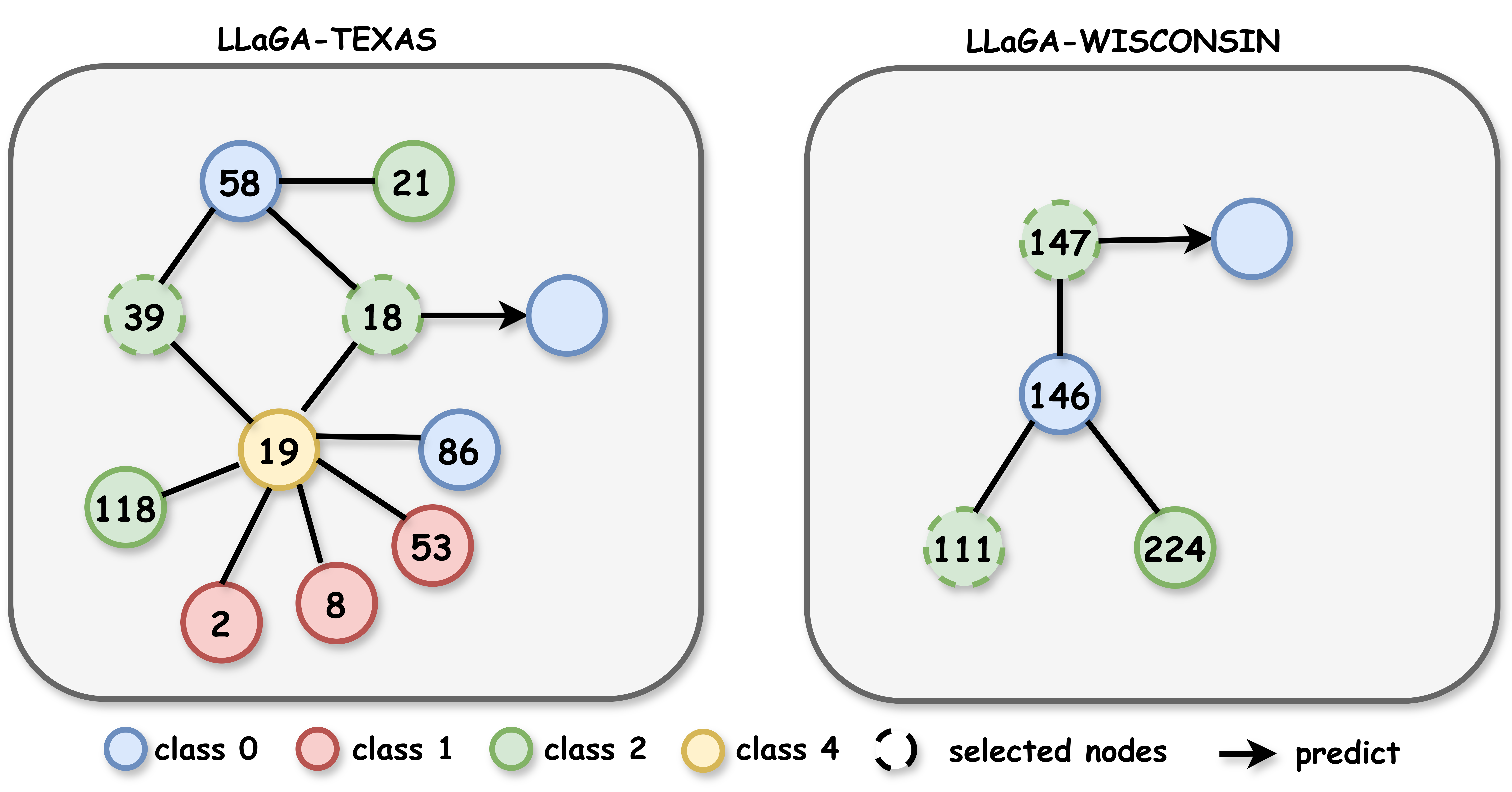
Figure 5: Examples demonstrating the interpretability of LGTL.

Appendix C Limitations and Impacts

C.1 Limitations

Here we provide discussions on limitations of our work. Currently, experiments of LGTL are primarily conducted on social and citation heterophilic graphs. In the future, we will extend LGTL to additional graph types (e.g., molecular interaction networks and knowledge graphs).Furthermore, we will investigate the integration of LGTL with emerging graph learning paradigms (e.g., dynamic graph and heterogeneous graphs) to address evolving challenges in graph representation.

C.2 Impacts

Positive Impacts. Our method enhances Tokenized Graph Learning Models (TGLMs) by improving the adaptability of token lists, which can broadly benefit real-world applications. For example, TGLMs are critical for analyzing social networks, recommendation systems, and bioinformatics. By enabling TGLMs to better handle diverse graph structures, our work may improve the accuracy and efficiency of these applications, supporting data-driven decision-making in fields like public health, urban planning, and e-commerce.

Negative Impacts. As a foundational methodological contribution, our work focuses on general graph machine learning research and we do not foresee that our work shall have major direct negative societal impacts.

Appendix D Propositions and Proofs of HO Template

D.1 Proof of Theorem 4.1

Base case k=0: By definition, $\mathbf{T}_{u,0}^{\text{HO}}=\mathbf{x}_{u}=\mathbf{H}_{u}^{0}$, so $\mathbf{M}_{0,0}^{\text{HO}}=1$ and $\mathbf{M}_{0,i}^{\text{HO}}=\mathbf{0}$ for $i>0$.

Base case k=1:

$$\mathbf{T}_{u,1}^{\text{HO}}=\frac{1}{n}\sum_{v\in\mathcal{N}_{u}^{1}}\mathbf{T}_{v,0}^{\text{HO}}=\frac{1}{n}\sum_{v\in\mathcal{N}_{u}^{1}}\mathbf{x}_{v}=\frac{1}{n}\mathbf{H}_{u}^{1}.$$ (11)

Thus, $\mathbf{T}_{u,1}^{\text{HO}}=\mathbf{M}_{1,1}^{\text{HO}}\mathbf{H}_{u}^{1}$, where $\mathbf{M}_{1,1}^{\text{HO}}=\frac{1}{n}$. For $i=0$, $\mathbf{M}_{1,0}^{\text{HO}}=\mathbf{0}$. This matches Rule 2 ($\mathbf{M}_{1,0}^{\text{HO}}=\mathbf{M}_{0,1}^{\text{HO}}=\mathbf{0}$) and Rule 4 ($\mathbf{M}_{1,1}^{\text{HO}}=\frac{1}{n}\left(\mathbf{M}_{0,0}^{\text{HO}}+(n-1)\mathbf{M}_{0,2}^{\text{HO}}\right)=\frac{1}{n}$).

Inductive step k=t: Assume $\mathbf{T}_{u,t-1}^{\text{HO}}=\sum_{i=0}^{t-1}\mathbf{M}_{t-1,i}^{\text{HO}}\mathbf{H}_{u}^{i}$ holds. For $\mathbf{T}_{u,t}^{\text{HO}}$:

$$\mathbf{T}_{u,t}^{\text{HO}}=\frac{1}{n}\sum_{v\in\mathcal{N}_{u}^{1}}\mathbf{T}_{v,t-1}^{\text{HO}}=\frac{1}{n}\sum_{v\in\mathcal{N}_{u}^{1}}\sum_{i=0}^{t-1}\mathbf{M}_{t-1,i}^{\text{HO}}\mathbf{H}_{v}^{i}.$$ (12)

By definition, $\sum_{v\in\mathcal{N}_{u}^{1}}\mathbf{H}_{v}^{i}=\mathbf{H}_{u}^{i+1}+(n-1)\mathbf{H}_{u}^{i-1}$. Substituting this into the equation:

$$\mathbf{T}_{u,t}^{\text{HO}}=\frac{1}{n}\left[\mathbf{M}_{t-1,0}^{\text{HO}}\mathbf{H}_{u}^{1}+\sum_{i=1}^{t-1}\mathbf{M}_{t-1,i}^{\text{HO}}\left(\mathbf{H}_{u}^{i+1}+(n-1)\mathbf{H}_{u}^{i-1}\right)\right].$$ (13)

Rearranging terms by $\mathbf{H}_{u}^{i}$:

$$\mathbf{T}_{u,t}^{\text{HO}}=\mathbf{M}_{t-1,1}^{\text{HO}}\mathbf{H}_{u}^{0}+\sum_{i=1}^{t}\frac{1}{n}\left(\mathbf{M}_{t-1,i-1}^{\text{HO}}+(n-1)\mathbf{M}_{t-1,i+1}^{\text{HO}}\right)\mathbf{H}_{u}^{i}.$$ (14)

This matches the recursive rules for $\mathbf{M}_{t,0}^{\text{HO}}$ and $\mathbf{M}_{t,i}^{\text{HO}}$ (Rules 2, 3, and 4). Thus, the induction holds.

D.2 Proposition1: Contributions Relate to the Parity of Hop

Proposition D.1 (Contributions Relate to the Parity of Hop).

For any $k\geq 0$, $\mathbf{T}_{u,k}^{\text{HO}}$ aggregates features exclusively from neighbors with hop counts of the same parity as $k$. Formally:

• For even $k=2m$: $\mathbf{M}_{2m,2n+1}^{\text{HO}}=\mathbf{0}$, $n\geq 0$, and $\mathbf{M}_{2m,2n}^{\text{HO}}\neq\mathbf{0}$, $0\leq n\leq m$;

• For odd $k=2m+1$: $\mathbf{M}_{2m+1,2n}^{\text{HO}}=\mathbf{0}$, $n\geq 0$, and $\mathbf{M}_{2m+1,2n+1}^{\text{HO}}\neq\mathbf{0}$, $0\leq n\leq m$.

Base Case k=0 and k=1:

• For $k=0$ (even), $\mathbf{T}_{u,0}^{\text{HO}}=\mathbf{x}_{u}$, so $\mathbf{M}_{0,0}^{\text{HO}}=1$ and $\mathbf{M}_{0,i}^{\text{HO}}=\mathbf{0}$ for $i>0$.

• For $k=1$ (odd), $\mathbf{T}_{u,1}^{\text{HO}}=\frac{1}{n}\sum_{v\in\mathcal{N}_{u}^{1}}\mathbf{x}_{v}$, so $\mathbf{M}_{1,1}^{\text{HO}}=\frac{1}{n}$ and $\mathbf{M}_{1,i}^{\text{HO}}=\mathbf{0}$ for $i\neq 1$.

Inductive Step k=t: Assume the property holds for $k=t$. Consider $k=t+1$:

• If $t$ is even ($t=2m$), then $t+1=2m+1$ (odd). By Rule 2 of Theorem 4.1, $\mathbf{M}_{2m+1,0}^{\text{HO}}=\mathbf{M}_{2m,1}^{\text{HO}}=\mathbf{0}$. For $i\geq 1$, $\mathbf{M}_{2m+1,i}^{\text{HO}}=\frac{1}{n}\left(\mathbf{M}_{2m,i-1}^{\text{HO}}+(n-1)\mathbf{M}_{2m,i+1}^{\text{HO}}\right)$. Since $\mathbf{M}_{2m,i-1}^{\text{HO}}$ and $\mathbf{M}_{2m,i+1}^{\text{HO}}$ are non-zero only if $i-1$ and $i+1$ are even (i.e., $i$ is odd), $\mathbf{M}_{2m+1,i}^{\text{HO}}$ is non-zero only when $i$ is odd.

• If $t$ is odd ($t=2m+1$), then $t+1=2m+2$ (even). By Rule 2 of Theorem 4.1, $\mathbf{M}_{2m+2,0}^{\text{HO}}=\mathbf{M}_{2m+1,1}^{\text{HO}}\neq\mathbf{0}$. For $i\geq 1$, $\mathbf{M}_{2m+2,i}^{\text{HO}}=\frac{1}{n}\left(\mathbf{M}_{2m+1,i-1}^{\text{HO}}+(n-1)\mathbf{M}_{2m+1,i+1}^{\text{HO}}\right)$. Since $\mathbf{M}_{2m+1,i-1}^{\text{HO}}$ and $\mathbf{M}_{2m+1,i+1}^{\text{HO}}$ are non-zero only if $i-1$ and $i+1$ are odd (i.e., $i$ is even), $\mathbf{M}_{2m+2,i}^{\text{HO}}$ is non-zero only when $i$ is even.

Thus, the property holds for all $k\geq 0$.

D.3 Proposition2: Monotonic Decay of Row Contributions

Proposition D.2 (Monotonic Decay of Row Contributions).

Within each row of $\mathbf{M}^{\text{HO}}$, nonzero contributions monotonically decay as the hop increases. Formally:

• For even $k=2m$: $\mathbf{M}_{2m,2i}^{\text{HO}}>\mathbf{M}_{2m,2(i+1)}^{\text{HO}}$, $0\leq i\leq m-1$;

• For odd $k=2m+1$: $\mathbf{M}_{2m+1,2i+1}^{\text{HO}}>\mathbf{M}_{2m+1,2(i+1)+1}^{\text{HO}}$, $0\leq i\leq m-1$.

Base Case m=0:

• For $k=0$ (even), the row has only $\mathbf{M}_{0,0}^{\text{HO}}=1$.

• For $k=1$ (odd), the row has only $\mathbf{M}_{1,1}^{\text{HO}}=\frac{1}{n}$.

Inductive Step m=t: Assume the property holds for $m=t$. Consider $m=t+1$:

• For even $k=2(t+1)$: By Rule 2 and Rule 4, $\mathbf{M}_{2(t+1),0}^{\text{HO}}=\mathbf{M}_{2t+1,1}^{\text{HO}}$. For $i\geq 1$,

  $$\mathbf{M}_{2(t+1),2i}^{\text{HO}}=\frac{1}{n}\left(\mathbf{M}_{2t+1,2i-1}^{\text{HO}}+(n-1)\mathbf{M}_{2t+1,2i+1}^{\text{HO}}\right).$$ (15)

  By the inductive hypothesis, $\mathbf{M}_{2t+1,2i-1}^{\text{HO}}<\mathbf{M}_{2t+1,2i-3}^{\text{HO}}$ and $\mathbf{M}_{2t+1,2i+1}^{\text{HO}}<\mathbf{M}_{2t+1,2i-1}^{\text{HO}}$, so

  $$\mathbf{M}_{2(t+1),2i}^{\text{HO}}<\frac{1}{n}\left(\mathbf{M}_{2t+1,2i-3}^{\text{HO}}+(n-1)\mathbf{M}_{2t+1,2i-1}^{\text{HO}}\right)=\mathbf{M}_{2(t+1),2(i-1)}^{\text{HO}}.$$ (16)

• For odd $k=2(t+1)+1$: By Rule 4,

  $$\mathbf{M}_{2(t+1)+1,2i+1}^{\text{HO}}=\frac{1}{n}\left(\mathbf{M}_{2(t+1),2i}^{\text{HO}}+(n-1)\mathbf{M}_{2(t+1),2(i+1)}^{\text{HO}}\right).$$ (17)

  By the inductive hypothesis, $\mathbf{M}_{2(t+1),2i}^{\text{HO}}<\mathbf{M}_{2(t+1),2(i-1)}^{\text{HO}}$ and $\mathbf{M}_{2(t+1),2(i+1)}^{\text{HO}}<\mathbf{M}_{2(t+1),2i}^{\text{HO}}$, so

  $$\mathbf{M}_{2(t+1)+1,2i+1}^{\text{HO}}<\mathbf{M}_{2(t+1)+1,2i-1}^{\text{HO}}.$$ (18)

Thus, the property holds for all $m\geq 0$.

D.4 Proposition3: Monotonic Decay of Column Contributions

Proposition D.3 (Monotonic Decay of Column Contributions).

Within each column of $\mathbf{M}^{\text{HO}}$, nonzero contributions monotonically decay as the token depth increases . Formally:

• For even $i=2j$: $\mathbf{M}_{2m,2j}^{\text{HO}}>\mathbf{M}_{2(m+1),2j}^{\text{HO}}$ for $0\leq j\leq m$;

• For odd $i=2j+1$: $\mathbf{M}_{2m+1,2j+1}^{\text{HO}}>\mathbf{M}_{2(m+1)+1,2j+1}^{\text{HO}}$ for $0\leq j\leq m$.

Base Case m=0:

• For $i=0$ (even), $\mathbf{M}_{0,0}^{\text{HO}}=1>\mathbf{M}_{2,0}^{\text{HO}}=\mathbf{M}_{1,1}^{\text{HO}}=\frac{1}{n}$.

• For $i=1$ (odd), $\mathbf{M}_{1,1}^{\text{HO}}=\frac{1}{n}>\mathbf{M}_{3,1}^{\text{HO}}=\frac{1}{n}\left(\mathbf{M}_{2,0}^{\text{HO}}+(n-1)\mathbf{M}_{2,2}^{\text{HO}}\right)=\frac{2n-1}{n^{3}}$.

Inductive Step m=t: Assume the property holds for $m=t$. Consider $m=t+1$:

• For even $i=2j$: By Rule 4,

  $$\mathbf{M}_{2(t+1),2j}^{\text{HO}}=\frac{1}{n}\left(\mathbf{M}_{2t+1,2j-1}^{\text{HO}}+(n-1)\mathbf{M}_{2t+1,2j+1}^{\text{HO}}\right)$$ (19)

  By the inductive hypothesis, $\mathbf{M}_{2t+1,2j-1}^{\text{HO}}>\mathbf{M}_{2t+3,2j-1}^{\text{HO}}$ and $\mathbf{M}_{2t+1,2j+1}^{\text{HO}}>\mathbf{M}_{2t+3,2j+1}^{\text{HO}}$, so $\mathbf{M}_{2(t+1),2j}^{\text{HO}}>\mathbf{M}_{2(t+2),2j}^{\text{HO}}$.

• For odd $i=2j+1$: By Rule 4,

  $$\mathbf{M}_{2(t+1)+1,2j+1}^{\text{HO}}=\frac{1}{n}\left(\mathbf{M}_{2(t+1),2j}^{\text{HO}}+(n-1)\mathbf{M}_{2(t+1),2(j+1)}^{\text{HO}}\right).$$ (20)

  By the inductive hypothesis, $\mathbf{M}_{2(t+1),2j}^{\text{HO}}>\mathbf{M}_{2(t+2),2j}^{\text{HO}}$ and $\mathbf{M}_{2(t+1),2(j+1)}^{\text{HO}}>\mathbf{M}_{2(t+2),2(j+1)}^{\text{HO}}$, so $\mathbf{M}_{2(t+1)+1,2j+1}^{\text{HO}}>\mathbf{M}_{2(t+2)+1,2j+1}^{\text{HO}}$.

Thus, the property holds for all $m\geq 0$. Then we have

$$\frac{\mathbf{M}_{k,k-2}^{\text{HO}}}{\mathbf{M}_{k,k}^{\text{HO}}}=(k-1)n-(k-2)>(k-2)(n-1).$$ (21)

Therefore, even within $\mathbf{T}_{u,k}^{\text{HO}}$, the far-hop neighbors are exponentially less influential than the near-hop ones.

D.5 Proof of Theorem 4.2

The Transformer’s attention mechanism aggregates value vectors $\mathbf{v}_{u}^{i}=\mathbf{T}_{u,i}^{\text{HO}}\mathbf{W}_{V}$ (with $\mathbf{W}_{V}$ as the value projection matrix) using the attention scores $\alpha_{i}$:

$$\sum_{i=0}^{L}\alpha_{i}\mathbf{v}_{u}^{i}=\sum_{i=0}^{L}\alpha_{i}\mathbf{T}_{u,i}^{\text{HO}}\mathbf{W}_{V}.$$ (22)

Substituting $\mathbf{T}_{u,i}^{\text{HO}}=\sum_{j=0}^{i}\mathbf{M}_{i,j}^{\text{HO}}\mathbf{H}_{u}^{j}$ (from 2) and $\mathbf{H}_{u}^{j}=\sum_{v\in\mathcal{N}_{u}^{j}}\mathbf{x}_{v}$ (sum of $j$-hop neighbor features), we get:

$$\sum_{i=0}^{L}\alpha_{i}\mathbf{v}_{u}^{i}$$ (23)

$$= \sum_{i=0}^{L}\alpha_{i}\mathbf{T}_{u,i}^{\text{HO}}\mathbf{W}_{V}$$

$$= \sum_{i=0}^{L}\alpha_{i}\sum_{j=0}^{i}(\mathbf{M}_{i,j}^{\text{HO}}\mathbf{H}_{u}^{j})\mathbf{W}_{V}$$

$$= \sum_{j=0}^{L}\left(\sum_{i=j}^{L}\alpha_{i}\mathbf{M}_{i,j}^{\text{HO}}\right)\left(\sum_{v\in\mathcal{N}_{u}^{j}}\mathbf{x}_{v}\right)\mathbf{W}_{V}.$$

By linearity of summation, the effective attention allocated to a specific $k$-hop neighbor $v\in\mathcal{N}_{u}^{k}$ is the coefficient of $\mathbf{x}_{v}\mathbf{W}_{V}$ in this expression. By Property 1 (parity restriction) of $\mathbf{M}_{i,k}^{\text{HO}}$, $\mathbf{M}_{i,k}^{\text{HO}}=\mathbf{0}$ when $i$ and $k$ have different parity. Thus, only terms with $i\equiv k\,\text{mod}\,2$ contribute:

$$\hat{\alpha}_{k}=\sum_{i=k}^{L}\alpha_{i}\mathbf{M}_{i,k}^{\text{HO}}=\sum_{i=k,\,i\equiv k\,\text{mod}\,2}^{L}\alpha_{i}\mathbf{M}_{i,k}^{\text{HO}}.$$ (24)

For property 1, given $k_{1}<k_{2}$ with $k_{1}\equiv k_{2}\,\text{mod}\,2$, consider the effective attention $\hat{\alpha}_{k_{1}}$ and $\hat{\alpha}_{k_{2}}$. By Property 2 (row monotonicity) of $\mathbf{M}_{i,k}^{\text{HO}}$, $\mathbf{M}_{i,k_{1}}^{\text{HO}}>\mathbf{M}_{i,k_{2}}^{\text{HO}}$ for all $i\geq k_{2}$. Thus:

$$\hat{\alpha}_{k_{1}}=\sum_{i=k_{1},\,i\equiv k_{1}\,\text{mod}\,2}^{L}\alpha_{i}\mathbf{M}_{i,k_{1}}^{\text{HO}}>\sum_{i=k_{2},\,i\equiv k_{2}\,\text{mod}\,2}^{L}\alpha_{i}\mathbf{M}_{i,k_{1}}^{\text{HO}}>\sum_{i=k_{2},\,i\equiv k_{2}\,\text{mod}\,2}^{L}\alpha_{i}\mathbf{M}_{i,k_{2}}^{\text{HO}}=\hat{\alpha}_{k_{2}}.$$ (25)

And for property 2, from the derivation of $\hat{\alpha}_{k}$, the effective attention allocated to a $k$-hop neighbor $v$ is the coefficient of $\mathbf{x}_{v}\mathbf{W}_{V}$ in the aggregated value vector:

$$\sum_{i=0}^{L}\alpha_{i}\mathbf{V}_{u}^{i}=\sum_{v\in\mathcal{V}}\hat{\alpha}_{v}\mathbf{x}_{v}\mathbf{W}_{V}.$$ (26)

For $v\in\mathcal{N}_{u}^{k}$, $\hat{\alpha}_{v}$ is determined by the sum of $\alpha_{i}\mathbf{M}_{i,k}^{\text{HO}}$ over $i\equiv k\,\text{mod}\,2$. Since $\mathbf{M}_{i,k}^{\text{HO}}$ and $\alpha_{i}$ are global to the token list (not dependent on individual nodes $v$), all $k$-hop neighbors $v_{1},v_{2}\in\mathcal{N}_{u}^{k}$ share the same $\hat{\alpha}_{k}$. Thus, $\hat{\alpha}_{v_{1}}=\hat{\alpha}_{v_{2}}=\hat{\alpha}_{k}$.

D.6 Proof of Theorem 4.3

We assume the existence of a linear classifier, parameterized by $W_{C}$, which satisfies the condition $\mathbf{H}^{0}\mathbf{W}_{C}=\mathbf{Y}$. We can express $\mathbf{H}^{0}=\mathbf{Y}\mathbf{W}_{C}^{-1}$.

Using the triangle inequality for Frobenius norms:

$$\left\|\mathbf{H}_{u}^{0}-\hat{\mathbf{A}}\mathbf{H}^{0}\right\|_{F}=\left\|\mathbf{H}_{u}^{0}-\sum_{i=0}^{L}\hat{\alpha}_{i}\sum_{v\in\mathcal{N}_{u}^{i}}\mathbf{H}_{v}^{0}\right\|_{F}\leq\sum_{i=0}^{L}\hat{\alpha}_{i}\sum_{v\in\mathcal{N}_{u}^{i}}\left\|\mathbf{H}_{u}^{0}-\mathbf{H}_{v}^{0}\right\|_{F}.$$ (27)

Assume raw features are Lipschitz continuous with respect to labels: $\left\|\mathbf{H}_{u}^{0}-\mathbf{H}_{v}^{0}\right\|_{F}\leq L\left\|\mathbf{y}_{u}-\mathbf{y}_{v}\right\|_{F}$ for the constant $L$. For one-hot labels, $\left\|\mathbf{y}_{u}-\mathbf{y}_{v}\right\|_{F}=\sqrt{2}$ if $\mathbf{y}_{u}\neq\mathbf{y}_{v}$, and $0$ otherwise. Thus:

$$\sum_{v\in\mathcal{N}_{u}^{i}}\left\|\mathbf{H}_{u}^{0}-\mathbf{H}_{v}^{0}\right\|_{F}\leq L\cdot\sqrt{2}\cdot|\{v\in\mathcal{N}_{u}^{i}\mid\mathbf{y}_{u}\neq\mathbf{y}_{v}\}|.$$ (28)

The number of $i$-hop neighbors with different labels is $|\mathcal{N}_{u}^{i}|(1-C_{u}^{i})$, where $C_{u}^{i}=\frac{|\{v\in\mathcal{N}_{u}^{i}\mid\mathbf{y}_{u}=\mathbf{y}_{v}\}|}{|\mathcal{N}_{u}^{i}|}$ is the label consistency ratio. Substituting this into the inequality:

$$\sum_{v\in\mathcal{N}_{u}^{i}}\left\|\mathbf{H}_{u}^{0}-\mathbf{H}_{v}^{0}\right\|_{F}\leq\sqrt{2}L\cdot|\mathcal{N}_{u}^{i}|(1-C_{u}^{i}).$$ (29)

Finally, substituting back into the smoothness bound:

$$\|\mathbf{H}_{u}^{0}-\hat{\mathbf{A}}\mathbf{H}^{0}\|_{F}\leq\sqrt{2}L\sum_{i=0}^{L}\hat{\alpha}_{i}|\mathcal{N}_{u}^{i}|(1-C_{u}^{i}).$$ (30)

Appendix E Details about ND

E.1 Definition and Recursive Properties of ND

Consider ND for the central node $u$, constructed via a fixed-shape computational tree of depth $L$ with neighbor sample size $n$ per hop. Let $L^{\prime}=\sum_{i=0}^{L}n^{i}$ denote the token list length. Define $\mathbf{M}_{i,j}^{\text{ND}}$ as the number of times $j$-hop neighbors of $u$ appear in the $i$-th layer of the token list (where layers are indexed by hop distance). The coefficients $\mathbf{M}_{i,j}^{\text{ND}}$ satisfy:

1. $\mathbf{M}^{\text{ND}}_{0,0}=1$ (root node, 0-hop).

2. $\mathbf{M}^{\text{ND}}_{1,0}=0$, $\mathbf{M}^{\text{ND}}_{1,1}=1$ (layer 1 contains only 1-hop neighbors).

3. $\mathbf{M}^{\text{ND}}_{k,0}=n\mathbf{M}^{\text{ND}}_{k-1,1}$.

4. For $i\geq 1$ and $j\geq 1$: $\mathbf{M}^{\text{ND}}_{i,j}=\mathbf{M}^{\text{ND}}_{i-1,j-1}+(n-1)\mathbf{M}^{\text{ND}}_{i-1,j+1}$.

Proof.

For $i=0$ (the root layer), ND contains only $u$ itself, so $\mathbf{M}^{\text{ND}}_{0,0}=1$ and $\mathbf{M}^{\text{ND}}_{0,j}=0$ for $j>0$. Rule 1 holds.
For $i=1$, since $u$ does not appear in layer 1, $\mathbf{M}^{\text{ND}}_{1,0}=0$; $\mathcal{N}_{u}^{1}$ appear exactly once per sampled node, so $\mathbf{M}^{\text{ND}}_{1,1}=1$. Rule 2 holds.
For 0-hop in general Layers ($i\geq 1$), the count of $\mathcal{N}_{u}^{0}$ in layer $k$ depends on the count of $\mathcal{N}_{u}^{1}$ in layer $k-1$. Each of the node in $\mathcal{N}_{u}^{1}$ in layer $k-1$ generates $n$ children in layer $k$, but $u$ itself appears as a parent of these children. Therefore, $\mathbf{M}^{\text{ND}}_{k,0}=n\mathbf{M}^{\text{ND}}_{k-1,1}$. Rule 3 holds.
For other hops in general Layers ($i\geq 1$), A $j$-th hop neighbor in layer $i$ can be derived from two sources: (1) A $(j-1)$-th hop neighbor in layer $i-1$ (parent node, contributing 1 occurrence), (2) $(j+1)$-th hop neighbors in layer $i-1$ (siblings of the parent node, contributing $(n-1)$ occurrences due to sampling). Therefore, $\mathbf{M}^{\text{ND}}_{i,j}=\mathbf{M}^{\text{ND}}_{i-1,j-1}+(n-1)\mathbf{M}^{\text{ND}}_{i-1,j+1}$. Rule 4 holds. ∎

E.2 Monotonicity Properties of ND

To characterize how ND distributes node occurrences across layers, we analyze the monotonicity of $\mathbf{M}^{\text{ND}}_{i,j}$. Specifically, we observe two critical monotonicity properties:

• Within-Layer Decay: $\mathbf{M}^{\text{ND}}_{i,j}>\mathbf{M}^{\text{ND}}_{i,j+2}$ for $\mathbf{M}^{\text{ND}}_{i,j}\neq 0$ (closer hops appear more frequently within a layer).

• Cross-Layer Growth: $\mathbf{M}^{\text{ND}}_{i,j}<\mathbf{M}^{\text{ND}}_{i+2,j}$ for $\mathbf{M}^{\text{ND}}_{i,j}\neq 0$ (deeper layers amplify the count of fixed-hop neighbors).

Proof.

By induction, assume $\mathbf{M}^{\text{ND}}_{i,j}>\mathbf{M}^{\text{ND}}_{i,j+2}$ holds for $i=t$ and any $j$. For $i=t+1$ and $j>0$:

$$\mathbf{M}^{\text{ND}}_{t+1,j}=\mathbf{M}^{\text{ND}}_{t,j-1}+(n-1)\mathbf{M}^{\text{ND}}_{t,j+1}>\mathbf{M}^{\text{ND}}_{t,j+1}+(n-1)\mathbf{M}^{\text{ND}}_{t,j+3}=\mathbf{M}^{\text{ND}}_{t+1,j+2}.$$ (31)

This follows from the inductive hypothesis $\mathbf{M}^{\text{ND}}_{t,j-1}>\mathbf{M}^{\text{ND}}_{t,j+1}$ and $\mathbf{M}^{\text{ND}}_{t,j+1}>\mathbf{M}^{\text{ND}}_{t,j+3}$.

And for $i=t+1$ and $j=0$:

$$\mathbf{M}^{\text{ND}}_{t+1,0}=n\mathbf{M}^{\text{ND}}_{t,1}>\mathbf{M}^{\text{ND}}_{t,1}+(n-1)\mathbf{M}^{\text{ND}}_{t,3}=\mathbf{M}^{\text{ND}}_{t+1,2}.$$ (32)

Therefore, Within-Layer Decay holds.

For Cross-Layer Growth, assume $\mathbf{M}^{\text{ND}}_{t,j}<\mathbf{M}^{\text{ND}}_{t+2,j}$ for $i=t$ and any $j$. For $i=t+2$:

$$\mathbf{M}^{\text{ND}}_{t+2,j}=\mathbf{M}^{\text{ND}}_{t+1,j-1}+(n-1)\mathbf{M}^{\text{ND}}_{t+1,j+1}>\mathbf{M}^{\text{ND}}_{t-1,j-1}+(n-1)\mathbf{M}^{\text{ND}}_{t-1,j+1}=\mathbf{M}^{\text{ND}}_{t,j}.$$ (33)

Therefore, Cross-Layer Growth holds.∎

E.3 Effective Attention Allocation of ND

Let $\alpha\in\mathbb{R}^{1\times L^{\prime}}$ denotes the attention scores assigned to the ND token list $\mathbf{T}^{\text{ND}}_{u,1},\mathbf{T}^{\text{ND}}_{u,2},\dots,\mathbf{T}^{\text{ND}}_{u,L^{\prime}}$ (normalized such that $\sum_{i=1}^{L^{\prime}}\alpha_{i}=1$). For a $k$-hop neighbor $v\in\mathcal{N}_{u}^{k}$ of $u$, the effective attention allocated to $v$ is:

$$\beta_{u,v}=\phi_{L,k}\cdot\alpha_{u,v},$$ (34)

where $\phi_{L,k}=\sum_{i=k,i\equiv k\,\text{mod}\,2}^{L}\mathbf{M}^{\text{ND}}_{i,k}$ is the weight of $k$-hop neighbors, and $\alpha_{u,v}$ is the direct attention score between $u$ and $v$.

Proof.

The aggregated value vector of ND is:

$$\sum_{i=1}^{L^{\prime}}\alpha_{i}\mathbf{V}_{i}$$ (35)

$$= \sum_{i=0}^{L}\sum_{k=0}^{i}\mathbf{M}^{\text{ND}}_{i,k}\sum_{v\in\mathcal{N}_{u}^{k}}\alpha_{u,v}V_{v}$$

$$= \sum_{k=0}^{L}(\sum_{i=k}^{L}\mathbf{M}^{\text{ND}}_{i,k})\sum_{v\in\mathcal{N}_{u}^{k}}\alpha_{u,v}V_{v}$$

$$= \sum_{k=0}^{L}\sum_{v\in\mathcal{N}_{u}^{k}}((\sum_{i=k,i\equiv k\,\text{mod}\,2}^{L}\mathbf{M}^{\text{ND}}_{i,k})\alpha_{u,v})\mathbf{x}_{v}W_{V},$$

where $\mathbf{V}_{j}$ is the value vector of the $j$-th $k$-hop neighbor. By definition, $\phi_{L,k}=\sum_{i=k}^{L}\mathbf{M}^{\text{ND}}_{i,k}$, so the effective attention $\beta_{u,v}=\phi_{L,k}\cdot\alpha_{u,v}$. ∎

E.4 Hop-Priority Bias in ND

This allocation exhibits two critical properties:

1. Near-Hop Dominance: $\phi_{L,k}>\phi_{L,k+2}$ for all $k\leq L$ (closer hops have higher total weights).

2. Layer Parity Bias:

   • If $L$ is odd ($L=2k+1$), odd hops ($k=1,3,\dots$) have $\phi_{L,k}>\phi_{L,k-1}$ and $\phi_{L,k}>(n-1)\phi_{L,k+1}$.

   • If $L$ is even ($L=2k$), even hops ($k=0,2,\dots$) have $\phi_{L,k}>\phi_{L,k-1}$ and $\phi_{L,k}>(n-1)\phi_{L,k+1}$.

Proof.

From within-layer decay, $\mathbf{M}^{\text{ND}}_{i,k}>\mathbf{M}^{\text{ND}}_{i,k+2}$ for all $i\geq k$. Therefore:

$$\phi_{L,k}=\sum_{i=k,i\equiv k\,\text{mod}\,2}^{L}\mathbf{M}^{\text{ND}}_{i,k}>\sum_{i=k,i\equiv k\,\text{mod}\,2}^{L}\mathbf{M}^{\text{ND}}_{i,k+2}=\phi_{L,k+2}.$$ (36)

Near-Hop Dominance holds.

For $L=2k+1$ (odd), consider $\phi_{L,2t+1}$:

$$\phi_{L,2t+1}$$ (37)

$$= \sum_{i=2t+1,i\equiv 2t+1\,\text{mod}\,2}^{2k+1}\mathbf{M}^{\text{ND}}_{i,2t+1}$$

$$= \sum_{i=2t,i\equiv 2t\,\text{mod}\,2}^{2k}\mathbf{M}^{\text{ND}}_{i,2t}+(n-1)\sum_{i=2t+2,i\equiv 2t+2\,\text{mod}\,2}^{2k}\mathbf{M}^{\text{ND}}_{i,2t+2}$$

$$= \phi_{L,2t}+(n-1)\phi_{L,2t+2}.$$

Therefore, $\phi_{L,2t+1}>\phi_{L,2t}$ and $\phi_{L,2t+1}>(n-1)\phi_{L,2t+2}$.

For $L=2k$ (even), consider $\phi_{L,2t+2}$:

$$\phi_{L,2t+2}$$ (38)

$$= \sum_{i=2t+2,i\equiv 2t+2\,\text{mod}\,2}^{2k}\mathbf{M}^{\text{ND}}_{i,2t+2}$$

$$= \sum_{i=2t+1,i\equiv 2t+1\,\text{mod}\,2}^{2k-1}\mathbf{M}^{\text{ND}}_{i,2t+1}+(n-1)\sum_{i=2t+3,i\equiv 2t+3\,\text{mod}\,2}^{2k-1}\mathbf{M}^{\text{ND}}_{i,2t+3}$$

$$= \phi_{L,2t+1}+(n-1)\phi_{L,2t+3}.$$

Therefore, $\phi_{L,2t+2}>\phi_{L,2t+1}$ and $\phi_{L,2t+2}>(n-1)\phi_{L,2t+3}$. Layer Parity Bias holds. ∎

E.5 Smoothness Bound of ND

Let $\hat{\mathbf{A}}\in\mathbb{R}^{1\times N}$ the attention vector for all nodes derived from ND. The smoothness of node $u$’s representation satisfies:

$$\|\mathbf{H}_{u}^{0}-\hat{\mathbf{A}}\mathbf{H}^{0}\|_{F}\leq\sqrt{2}L\frac{1}{1+\frac{1}{\frac{\sum_{i=0}^{L}\phi_{L,i}|\mathcal{N}^{i}_{u}|}{\sum_{i=0}^{L}\phi_{L,i}|\mathcal{N}^{i}_{u}|C_{u}^{i}}-1}\frac{\eta_{u}}{\gamma_{u}}},$$ (39)

where $\gamma_{u}=\mathbb{E}_{v\in\mathcal{N}_{u}^{i},\mathbf{y}_{u}=\mathbf{y}_{v}}\exp\left(\frac{\mathbf{q}_{u}\mathbf{k}_{v}^{\top}}{\sqrt{h}}\right)$, and $\eta_{u}=\mathbb{E}_{v\in\mathcal{N}_{u}^{i},\mathbf{y}_{u}\neq\mathbf{y}_{v}}\exp\left(\frac{\mathbf{q}_{u}\mathbf{k}_{v}^{\top}}{\sqrt{h}}\right)$.

Proof.

The smoothness metric of ND is:

$$\|\mathbf{H}_{u}^{0}-\hat{\mathbf{A}}\mathbf{H}^{0}\|_{F}=\left\|\mathbf{H}_{u}^{0}-\sum_{i=1}^{L^{\prime}}\alpha_{i}\mathbf{T}^{\text{ND}}_{u,i}\right\|_{F},$$ (40)

where $\alpha_{i}$ are the attention scores assigned to the tokens in ND.

By Theorem 9, each $k$-hop neighbor $v$ of $u$ appears $\phi_{L,k}$ times in the token list, with effective attention $\beta_{k,v}=\phi_{L,k}\cdot\alpha_{u,v}$. Thus, the aggregated token list can be rewritten as:

$$\sum_{i=1}^{L^{\prime}}\alpha_{i}\mathbf{T}^{\text{ND}}_{u,i}=\sum_{k=0}^{L}\sum_{v\in\mathcal{N}_{u}^{k}}\beta_{k,v}\mathbf{H}_{v}^{0}.$$ (41)

Using the Lipschitz assumption $\|\mathbf{H}_{u}^{0}-\mathbf{H}_{v}^{0}\|_{F}\leq L\|\mathbf{y}_{u}-\mathbf{y}_{v}\|_{F}$ and the one-hot label property $\|\mathbf{y}_{u}-\mathbf{y}_{v}\|_{F}=\sqrt{2}$ for $\mathbf{y}_{u}\neq\mathbf{y}_{v}$, we bound the smoothness metric:

$$\|\mathbf{H}_{u}^{0}-\hat{\mathbf{A}}\mathbf{H}^{0}\|_{F}\leq\sqrt{2}L\sum_{k=0}^{L}\sum_{v\in\mathcal{N}_{u}^{k},\mathbf{y}_{u}\neq\mathbf{y}_{v}}\beta_{k,v}.$$ (42)

Let $C_{u}^{k}=\frac{|\{v\in\mathcal{N}_{u}^{k}\mid\mathbf{y}_{u}=\mathbf{y}_{v}\}|}{|\mathcal{N}_{u}^{k}|}$ denote the label consistency of $k$-hop neighbors. The number of $k$-hop neighbors with different labels is $|\mathcal{N}_{u}^{k}|(1-C_{u}^{k})$. Substituting $\beta_{k,v}=\phi_{L,k}\cdot\alpha_{u,v}$, we get:

$$\sum_{v\in\mathcal{N}_{u}^{k},\mathbf{y}_{u}\neq\mathbf{y}_{v}}\beta_{k,v}=\phi_{L,k}\sum_{v\in\mathcal{N}_{u}^{k},\mathbf{y}_{u}\neq\mathbf{y}_{v}}.\alpha_{u,v}.$$ (43)

The attention scores $\alpha_{u,v}$ are softmax-normalized:

$$\alpha_{u,v}=\frac{\exp\left(\frac{\mathbf{q}_{u}\mathbf{k}_{v}^{\top}}{\sqrt{h}}\right)}{\sum_{v^{\prime}\in\mathbf{T}}\exp\left(\frac{\mathbf{q}_{u}\mathbf{k}_{v^{\prime}}^{\top}}{\sqrt{h}}\right)}.$$ (44)

The sum over $\alpha_{u,v}$ for differing labels becomes:

$$\sum_{v\in\mathcal{N}_{u}^{k},\mathbf{y}_{u}\neq\mathbf{y}_{v}}\alpha_{u,v}=\frac{|\mathcal{N}_{u}^{k}|(1-C_{u}^{k})\eta_{u}}{\sum_{i=0}^{L}\phi_{L,i}(|\mathcal{N}_{u}^{i}|C_{u}^{i}\gamma_{u}+|\mathcal{N}_{u}^{i}|(1-C_{u}^{i})\eta_{u})}.$$ (45)

Therefore, we bound the smoothness metric:

$$\|\mathbf{H}_{u}^{0}-\hat{\mathbf{A}}\mathbf{H}^{0}\|_{F}$$ (46)

$$\leq \sqrt{2}L\sum_{k=0}^{L}\sum_{v\in\mathcal{N}_{u}^{k},\mathbf{y}_{u}\neq\mathbf{y}_{v}}\beta_{k,v}$$

$$= \sqrt{2}L\sum_{k=0}^{L}\frac{\phi_{L,k}|\mathcal{N}_{u}^{k}|(1-C_{u}^{k})\eta_{u}}{\sum_{i=0}^{L}\phi_{L,i}(|\mathcal{N}_{u}^{i}|C_{u}^{i}\gamma_{u}+|\mathcal{N}_{u}^{i}|(1-C_{u}^{i})\eta_{u})}$$

$$= \sqrt{2}L\frac{1}{1+\frac{\sum_{i=1}^{L}\phi_{L,i}|\mathcal{N}_{u}^{i}|C_{u}^{i}}{\sum_{i=1}^{L}\phi_{L,i}|\mathcal{N}_{u}^{i}|(1-C_{u}^{i})}\frac{\eta_{u}}{\gamma_{u}}}$$

$$= \sqrt{2}L\frac{1}{1+\frac{1}{\frac{\sum_{i=1}^{L}\phi_{L,i}|\mathcal{N}_{u}^{i}|(1-C_{u}^{i})}{\sum_{i=1}^{L}\phi_{L,i}|\mathcal{N}_{u}^{i}|C_{u}^{i}}}\frac{\eta_{u}}{\gamma_{u}}}$$

$$= \sqrt{2}L\frac{1}{1+\frac{1}{\frac{\sum_{i=1}^{L}\phi_{L,i}|\mathcal{N}_{u}^{i}|}{\sum_{i=1}^{L}\phi_{L,i}|\mathcal{N}_{u}^{i}|C_{u}^{i}}-1}\frac{\eta_{u}}{\gamma_{u}}}.$$

∎

On homophilic graphs, where $C_{u}^{i}$ is uniformly high, the smoothness bound remains tight, enabling strong model performance. However, on heterophilic graphs, the structural bias of ND becomes critical: while $C_{u}^{i}$ increases with odd hop, the attention weight $\phi_{L,i}$ decreases with hop distance. This mismatch, where the model amplifies attention to near hops (with low $C_{u}^{i}$) and suppresses far hops (with high $C_{u}^{i}$), weakens the smoothness bound, limiting the model’s ability to learn meaningful representations. These theoretical findings align with the results of preliminary experiments (Table 1), where ND underperforms on heterophilic datasets due to this rigid hop-priority bias.

Appendix F Theoretical Analysis of LGTL

F.1 Adaptive Attention Aggregation with Gate Module

The attention given to the node $v$ in the $i$-th hop neighbors of node $u$ is:

$$\hat{\beta}_{u,i,v}=\hat{\alpha}_{u,i}\cdot\beta_{u,i,v}=\frac{\alpha_{u,i}\cdot\hat{\mathbf{s}}_{u,i}}{\langle\alpha_{u}\cdot\mathbf{s}_{u}\rangle}\cdot\beta_{u,i,v}.$$ (47)

Proof.

The aggregated value vector after adjustment is:

$$\sum_{i=0}^{L}\hat{\alpha}_{u,i}\mathbf{V}_{u}^{i}=\sum_{i=0}^{L}\hat{\alpha}_{u,i}\mathbf{T}_{u}^{i}\mathbf{W}_{V}.$$ (48)

Substituting $\mathbf{T}_{u}^{i}=\sum_{v\in\mathcal{G}_{u}^{i}}\beta_{u,i,v}\mathbf{H}_{v}^{0}$ and $\hat{\alpha}_{u,i}$, we get:

$$\sum_{i=0}^{L}\frac{\alpha_{u,i}\cdot\hat{\mathbf{s}}_{u,i}}{\langle\alpha_{u}\cdot\mathbf{s}_{u}\rangle}\sum_{v\in\mathcal{G}_{u}^{i}}\beta_{u,i,v}\mathbf{H}_{v}^{0}\mathbf{W}_{V}=\sum_{i=0}^{L}\sum_{v\in\mathcal{G}_{u}^{i}}\left(\frac{\alpha_{u,i}\cdot\hat{\mathbf{s}}_{u,i}}{\langle\alpha_{u}\cdot\mathbf{s}_{u}\rangle}\cdot\beta_{u,i,v}\right)\mathbf{H}_{v}^{0}\mathbf{W}_{V}.$$ (49)

This holds. ∎

F.2 Relationship with ND

ND scales the attention of the hops by $\phi_{L,k}=\sum_{i=k,i\equiv k\,\text{mod}\,2}^{L}\mathbf{M}^{\text{ND}}_{i,k}$, where $\mathbf{M}^{\text{ND}}_{i,k}$ is the hop matrix of ND. Therefore, $\hat{\beta}_{u,k,v}^{\text{ND}}=\phi_{L,k}\cdot\beta_{u,k,v}^{\text{ND}}$. For LGTL, setting $\mathcal{G}_{u}^{i}=\mathcal{N}_{u}^{i}$, $\beta_{u,k,v}=\beta_{u,k,v}^{\text{ND}}$, $\hat{\alpha}_{u,k}=\phi_{L,k}$ recovers the attention pattern of ND, i.e.,

$$s_{u,k}\propto\frac{\phi_{L,k}}{\alpha_{u,i}}$$ (50)

Therefore, ND is also a special case of LGTL.

F.3 Smooth Bound of LGTL

For simplicity of our analysis, assume that $\hat{\mathbf{s}}_{u,i}$ is the scores allocated to the $i$-th hop for the central node $u$, and $\sum_{i=0}^{L}\hat{\mathbf{s}}_{u,i}=L+1$, the Frobenius norm $\|\mathbf{H}_{u}^{0}-\hat{\mathbf{A}}\mathbf{H}^{0}\|_{F}$ is bounded by:

$$\|\mathbf{H}_{u}^{0}-\hat{\mathbf{A}}\mathbf{H}^{0}\|_{F}\leq\sqrt{2}L\frac{\sum_{i=0}^{L}\hat{\mathbf{s}}_{u,i}|\mathcal{G}_{u}^{i}|(1-C_{u}^{i})}{(\sum_{i=0}^{L}|\mathcal{G}_{u}^{i}|(1-C_{u}^{i}))+(\sum_{i=0}^{L}|\mathcal{G}_{u}^{i}|C_{u}^{i})\frac{\eta_{u}}{\gamma_{u}}}$$ (51)

Proof.

$$\|\mathbf{H}_{u}^{0}-\hat{\mathbf{A}}\mathbf{H}^{0}\|_{F}$$ (52)

$$\leq \sqrt{2}L\sum_{i=0}^{L}\hat{\mathbf{s}}_{u,i}\sum_{v\in\mathcal{G}_{u}^{i},y_{v}\neq y_{u}}\beta_{u,i,v}$$

$$= \sqrt{2}L\frac{(\sum_{i=0}^{L}\hat{\mathbf{s}}_{u,i}(\sum_{v\in\mathcal{G}_{u}^{i},y_{v}\neq y_{u}}1))\gamma_{u}}{(\sum_{i=0}^{L}(\sum_{v\in\mathcal{G}_{u}^{i},y_{v}\neq y_{u}}1))\gamma_{u}+(\sum_{i=0}^{L}(\sum_{v\in\mathcal{G}_{u}^{i},y_{v}=y_{u}}1))\eta_{u}}$$

$$= \sqrt{2}L\frac{(\sum_{i=0}^{L}\hat{\mathbf{s}}_{u,i}|\mathcal{G}_{u}^{i}|(1-C_{u}^{i}))\gamma_{u}}{(\sum_{i=0}^{L}|\mathcal{G}_{u}^{i}|(1-C_{u}^{i}))\gamma_{u}+(\sum_{i=0}^{L}|\mathcal{G}_{u}^{i}|C_{u}^{i})\eta_{u}}$$

$$= \sqrt{2}L\frac{\sum_{i=0}^{L}\hat{\mathbf{s}}_{u,i}|\mathcal{G}_{u}^{i}|(1-C_{u}^{i})}{(\sum_{i=0}^{L}|\mathcal{G}_{u}^{i}|(1-C_{u}^{i}))+(\sum_{i=0}^{L}|\mathcal{G}_{u}^{i}|C_{u}^{i})\frac{\eta_{u}}{\gamma_{u}}}.$$

∎

Analysis: If we directly aggregate all of the nodes from the $i$-th hop and allocate the same score for all hops, the bound is the same as graph transformers (Xing et al., 2024). Now we fix $|\mathcal{G}_{u}^{i}|$, we should assign high gate scores $\hat{\mathbf{s}}_{u}$ to hops with less label-inconsistent nodes, i.e., $|\mathcal{G}_{u}^{i}|(1-C_{u}^{i})$, to reduce the value of $\|\mathbf{H}_{u}^{0}-\hat{\mathbf{A}}\mathbf{H}^{0}\|_{F}$. However, we can not know which hop has a higher value of $C_{u}^{i}$. So, in general, $|\mathcal{G}_{u}^{i}|$ is the same for each hop. Let $|\mathcal{G}_{u}^{i}|=|G|$, and the smooth bouid is

$$\sqrt{2}L\frac{\sum_{i=0}^{L}\hat{\mathbf{s}}_{u,i}(1-C_{u}^{i})}{\sum_{i=0}^{L}(1-C_{u}^{i})+\frac{\eta_{u}}{\gamma_{u}}\sum_{i=0}^{L}C_{u}^{i}}.$$ (53)

So in order to reduce the value of $\|\mathbf{H}_{u}^{0}-\hat{\mathbf{A}}\mathbf{H}^{0}\|_{F}$, the higher $\hat{\mathbf{s}}_{u,i}$ will be assigned to the hop with the higher value of $C_{u}^{i}$, theoretically explaining the effectiveness of the gate module. Furthermore, if we allocate all scores to the hop with the highest $C_{u}^{i}$ (define as $C_{u}^{I}$), then we have:

$$\|\mathbf{H}_{u}^{0}-\hat{\mathbf{A}}\mathbf{H}^{0}\|_{F}\leq\mathcal{J}(1-C_{u}^{I}),$$ (54)

where $\mathcal{J}$ is a constant value, while the smooth bound of the predefined token lists and graph transformers is related to other task-irrelevant hops.

F.4 Special Cases: Frozen LLM and Hybrid Token Lists

F.4.1 Frozen LLM Adaptation

When using a frozen LLM, the attention mechanism cannot be fine-tuned. LGTL approximates the adjustment by scaling tokens directly:

$${\mathbf{T}}_{u}^{0}=\mathbf{s}_{u,0}\mathbf{H}_{u}^{0},\quad{\mathbf{T}}_{u}^{i}=\mathbf{s}_{u,i}\sum_{v\in\mathcal{G}_{u}^{i}}\beta_{u,i,v}\mathbf{H}_{v}^{0}.$$ (55)

The aggregated value vector becomes:

$$\sum_{i=0}^{L}{\alpha}_{u,i}V_{u}^{i}$$ (56)

$$= \sum_{i=0}^{L}{\alpha}_{u,i}{\mathbf{T}}_{u}^{i}\mathbf{W}_{V}$$

$$= \sum_{i=0}^{L}\sum_{v\in\mathcal{G}_{u}^{i}}({\alpha}_{u,i}\mathbf{s}_{u,i}\beta_{u,i,v})\mathbf{H}_{v}^{0}\mathbf{W}_{V}$$

$$= \sum_{i=0}^{L}({\alpha}_{u,i}\mathbf{s}_{u,i})\sum_{v\in\mathcal{G}_{u}^{i}}\beta_{u,i,v}\mathbf{H}_{v}^{0}\mathbf{W}_{V},$$

equivalent to applying $s_{u,i}$ as a multiplicative weight to each hop token.

F.4.2 Compatibility with Extended Token Lists (e.g., VCR-Graphormer)

A critical strength of LGTL is its plug-and-play compatibility with models that include additional tokens (e.g., cluster-based tokens in VCR-Graphormer). We formalize this compatibility below. Consider a model like VCR-Graphormer, where the token list includes $C$ cluster-based tokens. Let $\mathbf{C}^{j}$ denote the $j$-th cluster, and $p_{u,v}$ the Personalized PageRank score of node $v$ relative to $u$. The extended token list $\mathbf{T}_{u}^{\prime}$ is:

$$\begin{split}&\ \ \ \ \mathbf{T}_{u}^{0}=\mathbf{s}_{u,0}\cdot\mathbf{H}_{u}^{0}\\ &\quad\mathbf{T}_{u}^{i}=\mathbf{s}_{u,i}\cdot\sum_{v\in\mathcal{G}_{u}^{i}}\beta_{u,i,v}\mathbf{H}_{v}^{0}\ (i=1,\dots,L)\\ &\quad\mathbf{T}_{u}^{L+j}=\sum_{v\in\mathbf{C}^{j}}p_{u,v}\mathbf{H}_{v}^{0}\ (j=1,\dots,C).\end{split}$$ (57)

The model’s aggregated value vector using $\mathbf{T}_{u}$ is:

$$\sum_{i=0}^{L+C}\dot{\alpha}_{i}\cdot\mathbf{V}_{u}^{i}=\sum_{i=0}^{L+C}\dot{\alpha}_{i}\cdot\mathbf{T}_{u}^{i}\mathbf{W}_{V},$$ (58)

where $\mathbf{W}_{V}$ is the value projection matrix. Substituting $\mathbf{T}_{u}^{i}$:

$$=\sum_{i=0}^{L}\dot{\alpha}_{i}\cdot\mathbf{s}_{u,i}\cdot\left(\sum_{v\in\mathcal{G}_{u}^{i}}\beta_{u,i,v}\mathbf{H}_{v}^{0}\right)\mathbf{W}_{V}+\sum_{j=1}^{C}\dot{\alpha}_{L+j}\cdot\left(\sum_{v\in\mathbf{C}^{j}}p_{u,v}\mathbf{H}_{v}^{0}\right)\mathbf{W}_{V}.$$ (59)

The effective attention score for any node $v$ is:

$$\hat{\alpha}_{v}=\sum_{i=0}^{L}\left[v\in\mathcal{G}_{u}^{i}\right]\dot{\alpha}_{i}\cdot\mathbf{s}_{u,i}\cdot\beta_{u,i,v}+\sum_{j=1}^{C}\left[v\in\mathbf{C}^{j}\right]\dot{\alpha}_{L+j}\cdot p_{u,v},$$ (60)

where $[\cdot]$ is an indicator function. When cluster-based attention scores are zero ($\dot{\alpha}_{L+j}=0$), the model reduces to the base LGTL, confirming its compatibility as a drop-in plugin.

References

- Chen et al. [2024a] Runjin Chen, Tong Zhao, Ajay Jaiswal, Neil Shah, and Zhangyang Wang. Llaga: Large language and graph assistant. Forty-first International Conference on Machine Learning, 2024a.
- Shuman et al. [2013] David I Shuman, Sunil K Narang, Pascal Frossard, Antonio Ortega, and Pierre Vandergheynst. The emerging field of signal processing on graphs: Extending high-dimensional data analysis to networks and other irregular domains. IEEE signal processing magazine, 30(3):83–98, 2013.
- Kalofolias [2016] Vassilis Kalofolias. How to learn a graph from smooth signals. In Artificial intelligence and statistics, pages 920–929. PMLR, 2016.
- Xing et al. [2024] Yujie Xing, Xiao Wang, Yibo Li, Hai Huang, and Chuan Shi. Less is more: on the over-globalizing problem in graph transformers. Forty-first International Conference on Machine Learning, 2024.
- Kipf and Welling [2017] Thomas N Kipf and Max Welling. Semi-supervised classification with graph convolutional networks. International Conference on Learning Representations, 2017.
- Veličković et al. [2018] Petar Veličković, Guillem Cucurull, Arantxa Casanova, Adriana Romero, Pietro Lio, and Yoshua Bengio. Graph attention networks. International Conference on Learning Representations, 2018.
- Zhu et al. [2020] Jiong Zhu, Yujun Yan, Lingxiao Zhao, Mark Heimann, Leman Akoglu, and Danai Koutra. Beyond homophily in graph neural networks: Current limitations and effective designs. Advances in neural information processing systems, 33:7793–7804, 2020.
- Wu et al. [2022] Qitian Wu, Wentao Zhao, Zenan Li, David Wipf, and Junchi Yan. Nodeformer: A scalable graph structure learning transformer for node classification. In Advances in Neural Information Processing Systems, 2022.
- Chen et al. [2022a] Jinsong Chen, Kaiyuan Gao, Gaichao Li, and Kun He. Nagphormer: A tokenized graph transformer for node classification in large graphs. International Conference on Learning Representations, 2022a.
- Fu et al. [2024] Dongqi Fu, Zhigang Hua, Yan Xie, Jin Fang, Si Zhang, Kaan Sancak, Hao Wu, Andrey Malevich, Jingrui He, and Bo Long. Vcr-graphormer: A mini-batch graph transformer via virtual connections. In The Twelfth International Conference on Learning Representations, 2024.
- Yang et al. [2017] Cheng Yang, Maosong Sun, Wayne Xin Zhao, Zhiyuan Liu, and Edward Y Chang. A neural network approach to jointly modeling social networks and mobile trajectories. ACM Transactions on Information Systems (TOIS), 35(4):1–28, 2017.
- Huang et al. [2020] Kexin Huang, Cao Xiao, Lucas M Glass, Marinka Zitnik, and Jimeng Sun. Skipgnn: predicting molecular interactions with skip-graph networks. Scientific reports, 10(1):21092, 2020.
- Tang et al. [2024] Jiabin Tang, Yuhao Yang, Wei Wei, Lei Shi, Lixin Su, Suqi Cheng, Dawei Yin, and Chao Huang. Graphgpt: Graph instruction tuning for large language models. In Proceedings of the 47th International ACM SIGIR Conference on Research and Development in Information Retrieval, pages 491–500, 2024.
- Ouyang et al. [2022] Long Ouyang, Jeffrey Wu, Xu Jiang, Diogo Almeida, Carroll Wainwright, Pamela Mishkin, Chong Zhang, Sandhini Agarwal, Katarina Slama, Alex Ray, et al. Training language models to follow instructions with human feedback. Advances in neural information processing systems, 35:27730–27744, 2022.
- Ying et al. [2021] Chengxuan Ying, Tianle Cai, Shengjie Luo, Shuxin Zheng, Guolin Ke, Di He, Yanming Shen, and Tie-Yan Liu. Do transformers really perform badly for graph representation? Advances in neural information processing systems, 34:28877–28888, 2021.
- Vaswani et al. [2017] Ashish Vaswani, Noam Shazeer, Niki Parmar, Jakob Uszkoreit, Llion Jones, Aidan N Gomez, Łukasz Kaiser, and Illia Polosukhin. Attention is all you need. Advances in neural information processing systems, 30, 2017.
- Dwivedi and Bresson [2020] Vijay Prakash Dwivedi and Xavier Bresson. A generalization of transformer networks to graphs. AAAI 2021 Workshop on Deep Learning on Graphs: Methods and Applications, 2020.
- Mialon et al. [2021] Grégoire Mialon, Dexiong Chen, Margot Selosse, and Julien Mairal. Graphit: Encoding graph structure in transformers. arXiv preprint arXiv:2106.05667, 2021.
- Kreuzer et al. [2021] Devin Kreuzer, Dominique Beaini, Will Hamilton, Vincent Létourneau, and Prudencio Tossou. Rethinking graph transformers with spectral attention. Advances in Neural Information Processing Systems, 34:21618–21629, 2021.
- Wu et al. [2021] Zhanghao Wu, Paras Jain, Matthew Wright, Azalia Mirhoseini, Joseph E Gonzalez, and Ion Stoica. Representing long-range context for graph neural networks with global attention. Advances in neural information processing systems, 34:13266–13279, 2021.
- Chen et al. [2022b] Dexiong Chen, Leslie O’Bray, and Karsten Borgwardt. Structure-aware transformer for graph representation learning. In International conference on machine learning, pages 3469–3489. PMLR, 2022b.
- Kim et al. [2022] Jinwoo Kim, Dat Nguyen, Seonwoo Min, Sungjun Cho, Moontae Lee, Honglak Lee, and Seunghoon Hong. Pure transformers are powerful graph learners. Advances in Neural Information Processing Systems, 35:14582–14595, 2022.
- Rampášek et al. [2022] Ladislav Rampášek, Michael Galkin, Vijay Prakash Dwivedi, Anh Tuan Luu, Guy Wolf, and Dominique Beaini. Recipe for a general, powerful, scalable graph transformer. Advances in Neural Information Processing Systems, 35:14501–14515, 2022.
- Bo et al. [2023] Deyu Bo, Chuan Shi, Lele Wang, and Renjie Liao. Specformer: Spectral graph neural networks meet transformers. International Conference on Learning Representations, 2023.
- Ma et al. [2023] Liheng Ma, Chen Lin, Derek Lim, Adriana Romero-Soriano, Puneet K Dokania, Mark Coates, Philip Torr, and Ser-Nam Lim. Graph inductive biases in transformers without message passing. In International Conference on Machine Learning, pages 23321–23337, 2023.
- Shirzad et al. [2023] Hamed Shirzad, Ameya Velingker, Balaji Venkatachalam, Danica J Sutherland, and Ali Kemal Sinop. Exphormer: Sparse transformers for graphs. In International Conference on Machine Learning, pages 31613–31632, 2023.
- Chen et al. [2024b] Jinsong Chen, Hanpeng Liu, John Hopcroft, and Kun He. Leveraging contrastive learning for enhanced node representations in tokenized graph transformers. Advances in Neural Information Processing Systems, 37:85824–85845, 2024b.
- Zhang et al. [2024] Mengmei Zhang, Mingwei Sun, Peng Wang, Shen Fan, Yanhu Mo, Xiaoxiao Xu, Hong Liu, Cheng Yang, and Chuan Shi. Graphtranslator: Aligning graph model to large language model for open-ended tasks. In Proceedings of the ACM Web Conference 2024, pages 1003–1014, 2024.
- Ye et al. [2024] Ruosong Ye, Caiqi Zhang, Runhui Wang, Shuyuan Xu, and Yongfeng Zhang. Language is all a graph needs. Findings of the Association for Computational Linguistics, 2024.
- Li et al. [2018] Qimai Li, Zhichao Han, and Xiao-Ming Wu. Deeper insights into graph convolutional networks for semi-supervised learning. In Proceedings of the AAAI conference on artificial intelligence, volume 32, 2018.
- Nt and Maehara [2019] Hoang Nt and Takanori Maehara. Revisiting graph neural networks: All we have is low-pass filters. arXiv preprint arXiv:1905.09550, 2019.
- Oono and Suzuki [2019] Kenta Oono and Taiji Suzuki. Graph neural networks exponentially lose expressive power for node classification. International Conference on Learning Representations, 2019.
- Topping et al. [2021] Jake Topping, Francesco Di Giovanni, Benjamin Paul Chamberlain, Xiaowen Dong, and Michael M Bronstein. Understanding over-squashing and bottlenecks on graphs via curvature. International Conference on Learning Representations, 2021.
- Deac et al. [2022] Andreea Deac, Marc Lackenby, and Petar Veličković. Expander graph propagation. In Learning on Graphs Conference, pages 38–1, 2022.
- Hamilton et al. [2017] Will Hamilton, Zhitao Ying, and Jure Leskovec. Inductive representation learning on large graphs. Advances in neural information processing systems, 30, 2017.
- Xu et al. [2019] Keyulu Xu, Weihua Hu, Jure Leskovec, and Stefanie Jegelka. How powerful are graph neural networks? International Conference on Learning Representations, 2019.
- Namata et al. [2012] Galileo Namata, Ben London, Lise Getoor, Bert Huang, and U Edu. Query-driven active surveying for collective classification. In 10th international workshop on mining and learning with graphs, volume 8, page 1, 2012.
- Shchur et al. [2018] Oleksandr Shchur, Maximilian Mumme, Aleksandar Bojchevski, and Stephan Günnemann. Pitfalls of graph neural network evaluation. Relational Representation Learning Workshop, NeurIPS 2018, 2018.
- Pei et al. [2020] Hongbin Pei, Bingzhe Wei, Kevin Chen-Chuan Chang, Yu Lei, and Bo Yang. Geom-gcn: Geometric graph convolutional networks. International Conference on Learning Representations, 2020.
- Gasteiger et al. [2018] Johannes Gasteiger, Aleksandar Bojchevski, and Stephan Günnemann. Predict then propagate: Graph neural networks meet personalized pagerank. In International Conference on Learning Representations, 2018.
- Wu et al. [2019] Felix Wu, Amauri Souza, Tianyi Zhang, Christopher Fifty, Tao Yu, and Kilian Weinberger. Simplifying graph convolutional networks. In International conference on machine learning, pages 6861–6871. Pmlr, 2019.
- Chiang et al. [2023] Wei-Lin Chiang, Zhuohan Li, Ziqing Lin, Ying Sheng, Zhanghao Wu, Hao Zhang, Lianmin Zheng, Siyuan Zhuang, Yonghao Zhuang, Joseph E Gonzalez, et al. Vicuna: An open-source chatbot impressing gpt-4 with 90%* chatgpt quality. See https://vicuna. lmsys. org (accessed 14 April 2023), 2(3):6, 2023.
- Touvron et al. [2023] Hugo Touvron, Louis Martin, Kevin Stone, Peter Albert, Amjad Almahairi, Yasmine Babaei, Nikolay Bashlykov, Soumya Batra, Prajjwal Bhargava, Shruti Bhosale, et al. Llama 2: Open foundation and fine-tuned chat models. arXiv preprint arXiv:2307.09288, 2023.
- Chen et al. [2024c] Zhikai Chen, Haitao Mao, Hang Li, Wei Jin, Hongzhi Wen, Xiaochi Wei, Shuaiqiang Wang, Dawei Yin, Wenqi Fan, Hui Liu, et al. Exploring the potential of large language models (llms) in learning on graphs. ACM SIGKDD Explorations Newsletter, 25(2):42–61, 2024c.
- Huang et al. [2023] Jin Huang, Xingjian Zhang, Qiaozhu Mei, and Jiaqi Ma. Can llms effectively leverage graph structural information: When and why. In NeurIPS 2023 Workshop: New Frontiers in Graph Learning, 2023.
- Zhao et al. [2025] Jianan Zhao, Le Zhuo, Yikang Shen, Meng Qu, Kai Liu, Michael Bronstein, Zhaocheng Zhu, and Jian Tang. Graphtext: Graph reasoning in text space. NeurIPS Workshop: Adaptive Foundation Models, Evolving AI for Personalized and Efficient Learning, 2025.
- Tan et al. [2023] Yanchao Tan, Zihao Zhou, Hang Lv, Weiming Liu, and Carl Yang. Walklm: A uniform language model fine-tuning framework for attributed graph embedding. Advances in neural information processing systems, 36:13308–13325, 2023.
- Wang et al. [2024] Jianing Wang, Junda Wu, Yupeng Hou, Yao Liu, Ming Gao, and Julian McAuley. Instructgraph: Boosting large language models via graph-centric instruction tuning and preference alignment. Findings of the Association for Computational Linguistics ACL, 2024.
- Zhao et al. [2021] Jianan Zhao, Chaozhuo Li, Qianlong Wen, Yiqi Wang, Yuming Liu, Hao Sun, Xing Xie, and Yanfang Ye. Gophormer: Ego-graph transformer for node classification. arXiv preprint arXiv:2110.13094, 2021.
- Zhang et al. [2023] Ziwei Zhang, Haoyang Li, Zeyang Zhang, Yijian Qin, Xin Wang, and Wenwu Zhu. Graph meets llms: Towards large graph models. In NeurIPS 2023 Workshop: New Frontiers in Graph Learning, 2023.
- Ren et al. [2024] Xubin Ren, Jiabin Tang, Dawei Yin, Nitesh Chawla, and Chao Huang. A survey of large language models for graphs. In Proceedings of the 30th ACM SIGKDD Conference on Knowledge Discovery and Data Mining, pages 6616–6626, 2024.
- Li et al. [2024] Yuhan Li, Zhixun Li, Peisong Wang, Jia Li, Xiangguo Sun, Hong Cheng, and Jeffrey Xu Yu. A survey of graph meets large language model: progress and future directions. In Proceedings of the Thirty-Third International Joint Conference on Artificial Intelligence, pages 8123–8131, 2024.