On the creation of narrow AI:
hierarchy and nonlocality of neural network skills

Abstract

We study the problem of creating strong, yet narrow, AI systems. While recent AI progress has been driven by the training of large general-purpose foundation models, the creation of smaller models specialized for narrow domains could be valuable for both efficiency and safety. In this work, we explore two challenges involved in creating such systems, having to do with basic properties of how neural networks learn and structure their representations. The first challenge regards when it is possible to train narrow models from scratch. Through experiments on a synthetic task, we find that it is sometimes necessary to train networks on a wide distribution of data to learn certain narrow skills within that distribution. This effect arises when skills depend on each other hierarchically, and training on a broad distribution introduces a curriculum which substantially accelerates learning. The second challenge regards how to transfer particular skills from large general models into small specialized models. We find that model skills are often not perfectly localized to a particular set of prunable components. However, we find that methods based on pruning can still outperform distillation. We investigate the use of a regularization objective to align desired skills with prunable components while unlearning unnecessary skills.

1 Introduction

Today, the most competent AI systems in any particular domain are general systems that are relatively competent in every domain. The best models at math and coding are also broadly knowledgeable about a very diverse array of topics, from Roman history to home cooking recipes to medical diagnostics. And when domain-specific models are created today, they are typically general foundation models fine-tuned on a particular task, rather than new models trained from scratch (Ren et al., 2025; Kassianik et al., 2025), though with some notable exceptions (Hui et al., 2024). This state of affairs is convenient and powerful, since a single general model can be used for a variety of applications (Bommasani et al., 2021).

However, generality has downsides for both efficiency and safety. For instance, AI systems used as coding assistants possess a large amount of knowledge which is never needed in those applications. Instead, we might like to use smaller, specialized networks which preserve the coding knowledge of general systems without the same breadth of irrelevant knowledge. Narrow systems may also pose fewer safety risks than general systems. For instance, narrow systems may have fewer dangerous capabilities that pose CBRN risks (Barez et al., 2025), be easier to understand mechanistically (Bereska and Gavves, 2024; Sharkey et al., 2025), or be easier to verify properties of (Tegmark and Omohundro, 2023; Dalrymple et al., 2024; Tegmark et al., 2025). More imaginatively, for systems to operate autonomously in the world requires a large breadth of skills, and an ecosystem of narrow “tool AI” systems may therefore reduce loss-of-control risks and better support human agency over the long term (Drexler, 2019).

In this work, we investigate some basic questions about how neural networks learn and represent skills that are relevant to the problem of creating narrow AI systems. As summarized in Figure˜1, we focus on two main themes. First, we consider the question of when it is possible to train well-performing neural networks from scratch on a narrow data distribution. Through experiments on a novel synthetic task with hierarchical structure, we find that it can be necessary to train networks on a broad distribution to efficiently learn narrow tasks within that distribution. These results contribute to a growing literature on how task structure influences neural network learning dynamics Ramesh et al. (2023); Okawa et al. (2023); Park et al. (2024); Abbe et al. (2023), but with special relevance to the problem of creating narrow AI. Second, we consider the question of whether one can use pruning to turn broad networks into smaller narrow ones. We find that the nonlocality of network representations to prunable model components poses a challenge for this goal. While distributed representations have been extensively studied in the context of neural network interpretability Bricken et al. (2023) and in the classical connectionist literature (Smolensky, 1990; Hinton, 1986), we study how this property of neural network computation impacts pruning and unlearning Barez et al. (2025) for creating narrow AI. Our specific contributions are as follows:

Figure 1: We study two challenges to making strong, narrow-purpose AI models. (A): Data may have hierarchical structure. If skills have a hierarchical dependence, where some skills are only learnable after more primitive skills are learned first, then it sometimes may be necessary to train on a broad distribution of data to learn certain narrow skills within that distribution. These dynamics may mean that general-purpose models must be trained to achieve certain performance on some domains. (B): Model features are distributed. By default, skills may not be localizable to a particular set of model components (e.g. neurons). In this case, pruning of model components won’t precisely retain wanted skills and remove unwanted skills from models. We explore methods for aligning the model features relevant to particular domains with a smaller subset of model components while unlearning others.

• We describe a synthetic task, compositional multitask sparse parity (CMSP), extending the multitask sparse parity task of Michaud et al. (2023). We find that networks trained on this task exhibit extremely strong curriculum learning effects, where it is necessary to train on a broad distribution of tasks in order to learn certain other tasks.

• We study pruning and unlearning on our networks trained on CMSP. We observe that tasks are often distributed and distinct subtasks are entangled, making pruning an imperfect strategy for “narrowing” the breadth of network skills. However, we find that a simple group-sparsity regularization objective can be used to sparsify networks and unlearn skills.

• We perform an empirical comparison of methods for creating narrow systems on MNIST and in LLMs. We tentatively find that methods based on pruning outperform distillation and training networks from scratch for the creation of smaller, more narrow systems.

This work is organized as follows. In Section˜2, we briefly describe methods. In Section˜3 we perform a detailed case study of training and pruning on the CMSP task. We define the task (Section˜3.1), study network training dynamics on it (Section˜3.2), find distributed representations in these networks (Section˜3.3), and use a regularization method for pruning and unlearning in these networks (Section˜3.4). We then compare various methods for creating narrow models, studying MNIST in Section˜4 and language models in Section˜5. We discuss related work in Section˜6 and conclude in Section˜7.

2 Methods

Pruning: We aim to preserve the performance of a model $f(\cdot;\theta)$ on a distribution $\mathcal{D}_{N}$ while pruning model components. Let $g$ be a collection of parameter indices $i$ corresponding to prunable components of the model (e.g. the in-weights and out-weights of a neuron), and let $G$ denote the collection of all such groups. After ablating a specific $g$, we denote the new parameters $\theta_{g}^{*}$. To perform pruning, for each $g\in G$, we compute an ablation score $s_{g}=\big{|}\mathbb{E}_{(x,y)\in\mathcal{D}_{N}}\big{[}L(f(x;\theta),y)-L(f(x;\theta_{g}^{*}),y)\big{]}\big{|}$, the absolute change in the model’s expected loss $L$ after pruning $g$. We sort groups by their ablation score and prune greedily to the desired sparsity from lowest to highest ablation score. Where feasible, we estimate $s_{g}$ empirically by manually ablating the group across many samples from $\mathcal{D}_{N}$. When this is computationally intractable, we instead use a linear estimate which we refer to as an attribution score after Nanda (2023); Syed et al. (2023): $\hat{s}_{g}=\big{|}\sum_{i\in g}\frac{\partial L}{\partial\theta_{i}}(-\theta_{i})\big{|}=|\frac{\partial L}{\partial\theta}\cdot(\theta_{g}^{*}-\theta)|$, where $\partial L/\partial\theta$ is the model’s gradient on the distribution $\mathcal{D}_{N}$, which can be computed once and reused for all $g\in G$.
Regularization: We also experiment with making networks more prunable by performing additional training with a “group lasso” regularization penalty on the model weights Tibshirani (1996); Yuan and Lin (2006); Wen et al. (2016); Zhou et al. (2016). The group lasso penalty $R$ is the L1 norm of the L2 norms of each parameter group: $R(\theta)=\sum_{g\in G}\sqrt{\sum_{i\in g}\theta_{i}^{2}}$. This penalty incentivizes the weights to become sparse at the level of entire groups $g$. When we perform “group lasso training” on a distribution $\mathcal{D}_{N}$, we minimize the loss $\mathbb{E}_{(x,y)\sim\mathcal{D}_{N}}[L(f(x;\theta),y)+\lambda R(\theta)]$.
Distillation: We also explore distilling knowledge from a teacher model using the standard algorithm employed in Hinton et al. (2015), minimizing the KL divergence between student and teacher output distributions.

3 Case study: compositional multitask sparse parity

In this section, we conduct a detailed study of both curriculum learning and pruning on simple synthetic task, which we call compositional multitask sparse parity (CMSP).

3.1 Defining compositional multitask sparse parity (CMSP)

The compositional multitask sparse parity (CMSP) task is a simple extension of the sparse parity task recently studied in Barak et al. (2022) and the multitask sparse parity task studied in Michaud et al. (2023), described below.

Barak et al. (2022) studied neural network training dynamics on the sparse parity (SP) task. This is a binary classification problem on binary strings $x$ of length $n$, where the label of a given sample $x$ is the parity of the bits at a subset $I$ of $k$ indices: $y=\oplus_{l=1}^{k}x[I_{l}]$. Strings $x$ are sampled uniformly. Barak et al. observed that the loss curve for neural networks trained on this task exhibits a sharp drop after an initial plateau, a case of the sort of “emergence” which has been observed in LLMs (Wei et al., 2022; Olsson et al., 2022) and in other toy settings (Nanda et al., 2023).

Michaud et al. (2023) extended the task to multitask sparse parity (MSP). In the MSP problem, input strings consist of $m+n$ bits, where the first $m$ bits are called “control bits” and the last $n$ bits are called “task bits”. These leading $m$ control bits encode which “subtask” must be solved in each problem instance. Instead of a single length-$k$ set of indices $I$, a collection of $m$ sets of task bit indices (typically of equal length $k$) is chosen $\{I_{1},\ldots,I_{m}\}$. For each sample, only one control bit is ON (1) while the others are OFF (0). If control bit $t$ is ON, then that sample’s label is the parity of bits $I_{t}$: $y=\oplus_{l=1}^{k}x[(I_{t})_{l}]$. Michaud et al. (2023) found that when subtasks are power law distributed in frequency, where the probability that control bit $i$ is ON is $p_{i}\propto i^{-(\alpha+1)}$,

the mean loss exhibits power-law scaling Hestness et al. (2017); Kaplan et al. (2020) while individual subtasks are learned at different times proportional to their frequency. They conjecture that LLM learning dynamics may be similar.

One of the main limitations of the MSP task, and the associated model of neural scaling from Michaud et al. (2023), is that subtasks are independent. However, the world, and the problem of learning from it, intuitively has a hierarchical structure—in order to learn to do certain concepts and tasks, we must first learn simpler concepts and tasks. Accordingly, humans are taught in a curriculum, where simpler concepts and tasks are learned first, and then composed into more complex ones later. To capture this structure, we now introduce the toy task compositional multitask sparse parity (CMSP). We show some CMSP samples to the right:

CMSP is similar to MSP, except that (1) we require subtask indices to be disjoint: $I_{i}\cap I_{j}=\emptyset$ if $i\neq j$, and (2) multiple control bits can now be ON at the same time, in which case the label is the parity of the bits in the union of the indices for each subtask. If control bits $i,j$ are both ON, the label is the parity of the task bits at indices $I_{i}\cup I_{j}$. We call samples for which only one control bit is ON “atomic” and samples for which multiple control bits are ON “composite”. So if $k=3$ for all subsets $I_{i}$, then on atomic samples networks must compute the parity of $3$ input bits, on composite samples with two control bits ON the label is the parity of $6$ input bits, and so on. Above, we illustrated some CMSP data samples with $m=3$, $n=9$, and $k=3$.

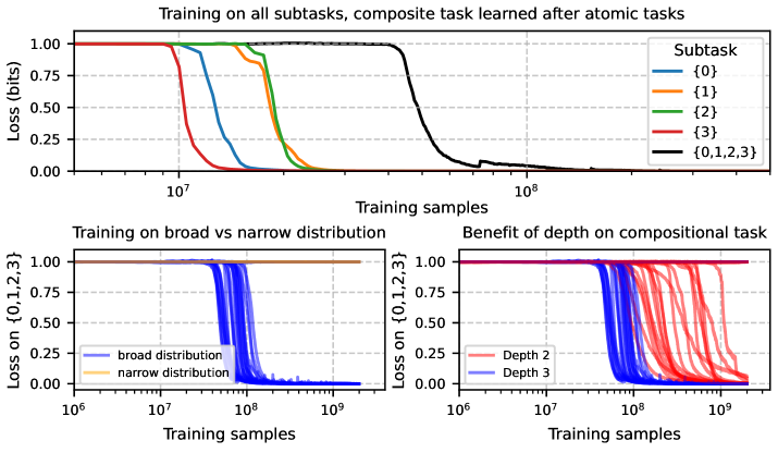
Figure 2: Training dynamics on compositional multitask sparse parity. Top: training dynamics for a single network trained on four atomic subtasks {0}, {1}, {2}, {3}, and their composition {0,1,2,3}. Bottom left: loss on compositional subtask {0,1,2,3}, when training only on samples from that task vs. also training on atomic subtasks. We see that by training on a broader distribution, we are able to learn the narrow task much faster and more reliably than when only training on samples from the narrow task. Bottom right: When training on the full distribution, deeper networks learn the compositional task faster and more reliably than networks with a single hidden layer. We report the minimum loss within the previous 100 steps of training to filter out loss spikes.

3.2 Learning dynamics on CMSP

We find that neural network training on CMSP exhibits extremely strong curriculum learning effects. To denote different types of CMSP samples, we list the ON control bits for those samples. So, given a choice of $m,n,k$ and $I_{1},\ldots,I_{m}$, $\mathcal{D}_{\{0\}}$ denotes all samples for atomic subtask 0, and $\mathcal{D}_{\{0,1,2,3\}}$ denotes all samples from the composite subtask where the first four control bits are ON. For each subtask, there are $2^{n}$ possible samples in that subtask, since the $m$ control bits are fixed but the $n$ task bits are free.

We first train ReLU MLPs with 1-2 hidden layers of width 128 with the Adam optimizer on CMSP samples with $m=4$, $n=64$, $k=4$, and 2000 samples per task (atomic or composite) per batch. We show the learning dynamics of these networks in Figure˜2. We find that when we train on a dataset containing both atomic and compositional samples $\mathcal{D}_{\{0\}}\cup\mathcal{D}_{\{1\}}\cup\mathcal{D}_{\{2\}}\cup\mathcal{D}_{\{3\}}\cup\mathcal{D}_{\{0,1,2,3\}}$ in equal proportion, atomic tasks are learned before composite ones.

Something interesting happens however when we remove atomic samples from the dataset: we find that learning composite tasks takes dramatically longer. When we train on $\mathcal{D}_{\{0\}}\cup\mathcal{D}_{\{1\}}\cup\mathcal{D}_{\{2\}}\cup\mathcal{D}_{\{3\}}\cup\mathcal{D}_{\{0,1,2,3\}}$ with 10000 samples per batch (2000 per subtask), across 40 seeds, we find that 27/40 networks converge on composite subtask $\mathcal{D}_{\{0,1,2,3\}}$ within $2\times 10^{9}$ samples, and the networks that do converge typically converge within $2\times 10^{8}$ samples. However, when we train just on $\mathcal{D}_{\{0,1,2,3\}}$, with a batch size of 2000 samples, we find that 0/40 networks converge within $2\times 10^{9}$ samples in Figure˜2 (bottom left). It is much more efficient to train on a broader distribution in order to learn subtask $\mathcal{D}_{\{0,1,2,3\}}$ than just training on $\mathcal{D}_{\{0,1,2,3\}}$ on its own.

This result makes sense given the exponential hardness of learning parities (Shoshani and Shamir, 2025). One explanation of these results is that networks compute the parity of the atomic subtask bits in the first hidden layer, and then to learn the composite subtask they compute the parity of these values in the second layer. This way, the network never needs to directly learn the parity of 16 bits, and learning the composite subtask is akin to computing the parity of 4 bits. We find that there is indeed a learning advantage to depth: when we train on $\mathcal{D}_{\{0\}}\cup\mathcal{D}_{\{1\}}\cup\mathcal{D}_{\{2\}}\cup\mathcal{D}_{\{3\}}\cup\mathcal{D}_{\{0,1,2,3\}}$ networks with 2 hidden layers are able to learn the composite task somewhat more reliably (27/40 seeds converged with depth 3 versus 19 with depth 2) but, more significantly, they learn much faster than networks with only a single hidden layer. In Figure˜7, we confirm that this effect is likely not just due to differences in network parameter count. This result may also provide some explanation for advantage of depth in deep learning – not only is depth necessary for networks to efficiently approximate certain functions (Lin et al., 2017), we find here that depth is helpful to efficiently learn tasks with hierarchical structure.

These sorts of dynamics may be a part of the explanation for why large-scale general-purpose models perform so strongly at many narrow, valuable tasks. We want to emphasize, however, that the toy task where we observe these curriculum effects is fairly contrived. It is not clear to what extent there are similarly strong effects on real-world tasks, and in many domains it is in fact possible to train narrow specialized models by only training on data in that domain. For instance, self-driving cars do not need to be trained on a broad corpus of text like LLMs.

Our work shows that for some types of tasks, it may be necessary to train on a broad data distribution in order to learn some subtasks efficiently. Accordingly, we now turn to the question of how to efficiently transfer knowledge from large models into smaller specialized ones.

3.3 Nonlocal representations in CMSP networks

If the circuitry for some subtasks were localized to a particular set of neurons, and the circuitry for other subtasks were localized to different neurons, then the task of specializing broad networks into narrow ones would be trivial. One could simply prune away neurons (or other model components, e.g. attention heads in transformers) associated with some subtasks, and keep others. However, often the situation seems more complicated than this ideal, which will be a focus for the rest of this paper.

A related problem has recently been studied in neural network interpretability, where it has been observed that individual computational units in neural networks, such as neurons, are polysemantic, activating across a wide variety of unrelated inputs (Olah et al., 2017; Elhage et al., 2022). Accordingly, many assume that the true model “features” do not align with architectural components like neurons. Multiple explanations have been proposed for this phenomenon. One is simply that the model architecture does not always “privilege” a particular basis (Elhage et al., 2021, 2023), though other incidental reasons for polysemanticity have also been proposed (Lecomte et al., 2023). Another explanation of polysemanticity is the superposition hypothesis (Arora et al., 2018; Elhage et al., 2022). The superposition hypothesis suggests that the need to represent more features than there are dimensions or neurons prevents features from being represented as orthogonal directions in the feature space, and therefore all features cannot be aligned with standalone model dimensions or neurons. Recently, studies that use sparse autoencoders to identify monosemantic model features have found that most features are highly distributed across a large number of dimensions of activation space (Bricken et al., 2023).

In our CMSP networks, we observe a related problem. By default, without any explicit regularization, there is no incentive for the network to localize certain circuits cleanly into a particular set of neurons. We train networks with two hidden layers on a dataset of CMSP samples with $m=6$, $n=18$, $k=3$ with two different skill trees: {0}, {1}, {2}, {0,1,2}, and {3}, {4}, {5}, {3,4,5} until convergence. In Figure˜3, we visualize the connectivity of a 2-hidden-layer MLP trained on this dataset, and see that the network is densely connected without obvious structure.

We attempt to prune this network to retain performance on subtask {0,1,2} while unlearning {3,4,5}. With MLPs, our groups of parameters $g$ are the in-weights, bias, and out-weights for each hidden layer neuron, so that $|G|$ is the total number of hidden neurons. We compute ablation scores on the distribution $\mathcal{D}_{N}=\mathcal{D}_{\{0,1,2\}}$ (estimated on 2000 samples) and prune greedily, as described in Section˜2. In Figure˜3, we show accuracy on subtask {0,1,2} vs. sparsity with this pruning strategy. When applied naively, network performance tends to degrade quickly, since without explicit regularization the network is not optimized to be naively prunable (see in Appendix Figure˜8 and Figure˜9 for more on how ablation scores for each subtask vary across neurons). However, when we perform an additional 1000 steps of training on $\mathcal{D}_{\{0,1,2\}}$ (5000 samples per batch) after pruning (after either removing neurons from the architecture or pinning pruned weights at zero) we can recover performance at higher sparsity levels. Since we are training just on compositional samples, 1000 steps is not enough to re-learn this task on its own, so if we can recover performance, that will be because the mechanisms for the task were somewhat preserved after pruning. We observe that often, the tasks {0,1,2} and {3,4,5} are entangled – when we prune as aggressively as we can while being able to recover performance on subtask {0,1,2}, we can often still recover some performance on subtask {3,4,5}. However, for our CMSP networks the degree of entanglement is highly seed-dependent, and sometimes the subtasks are disentangled enough that pruning as aggressively as possible on one subtask does robustly unlearn the other. We show pruning curves across seeds and widths in Appendix Figure˜10.

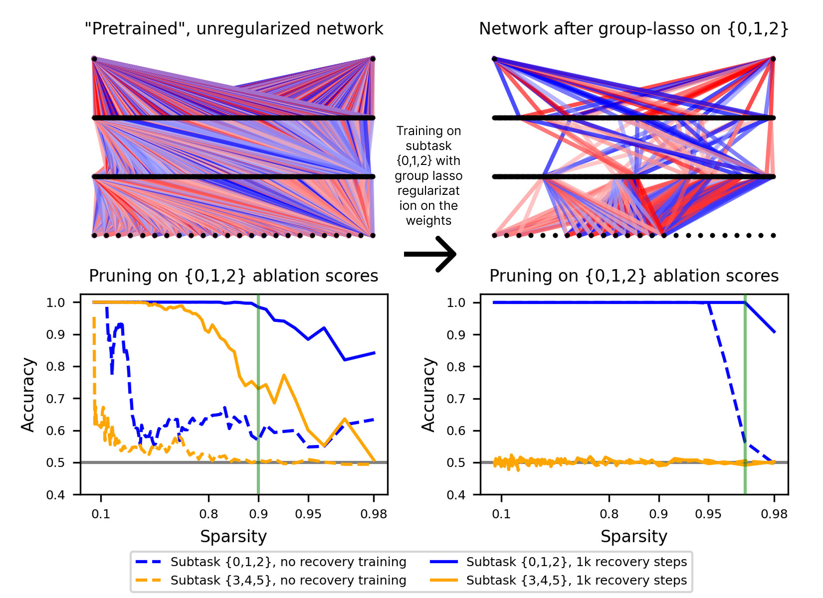
Figure 3: Top: We visualize the connectivity of 2-hidden-layer MLPs trained on a CMSP distribution with subtasks {0}, {1}, {2}, {0,1,2}, {3}, {4}, {5}, {3,4,5}, visualized before (left) and after (right) regularizing network weights with the group lasso sparsity penalty while training on subtask {0,1,2}. We find that network connectivity becomes sparse after regularizing. Bottom: we show how pruning affects task performance on subtasks {0,1,2} and {3,4,5} at varying sparsity levels. We prune neurons based on the absolute change that ablating them has on the loss on subtask {0,1,2}. We find that subtasks here are nonlocal and entangled in the “pretrained” network (left). As we prune neurons according to their relevance on subtask {0,1,2}, at the sparsity at which performance on subtask {0,1,2} accuracy drops below 98% (green line), we can still recover some performance on subtask {3,4,5} with a small amount of additional training. Thus naive pruning here has not completely and robustly unlearned subtask {3,4,5}. However, after regularizing the weights (right), we find that not only we can more aggressively prune the network, but we have also robustly unlearned subtask {3,4,5}. Note that the degree to which subtasks are nonlocal and entangled in the pretrained networks depends on seed and width, and we show a variety of additional curves in Figure˜10.

3.4 Regularizing to “narrow” networks

We find that we can use a simple regularization penalty to simultaneously unlearn some tasks while incentivizing the network to move its features to be less distributed, allowing for more aggressive pruning. As described in Section˜2, we simply perform additional training on $\mathcal{D}_{\{0,1,2\}}$ with a group lasso sparsity penalty on the network weights. We aim for this penalty to “clean up” circuitry Varma et al. (2023) not relevant to prediction on $\mathcal{D}_{\{0,1,2\}}$ while also sparsifying the weights across groups of parameters, allowing for easier pruning.

We apply this regularization to our CMSP networks, training with penalty strength $\lambda=10^{-3}$ with a batch size of 2000 for 10000 steps. With this regularized network, we then re-compute neuron ablation scores and prune. In Figure˜3 we find that, in CMSP networks, this method is effective at unlearning skills and making the network more prunable. We find that we can prune more aggressively while retaining performance on subtask {0,1,2}, and we are not able to recover performance on {3,4,5} at any sparsity level.

4 Pruning vs distillation: MNIST

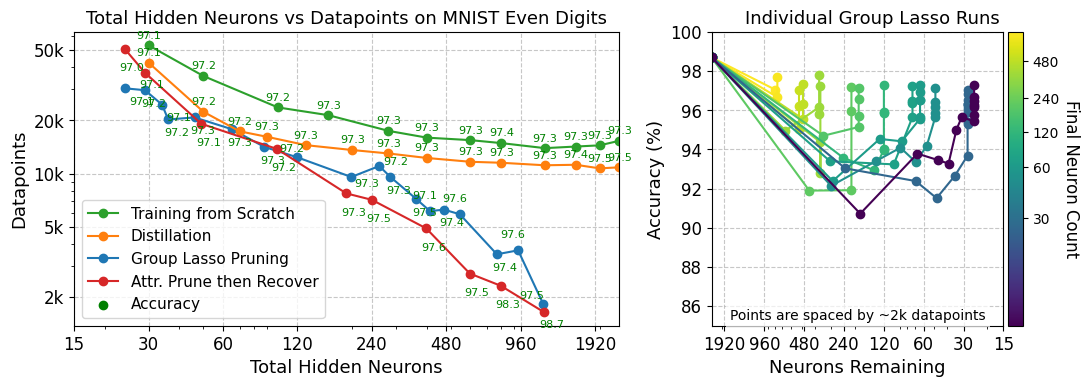
Figure 4: Left: We compare the performance of distillation, training from scratch, and two pruning approaches for creating small networks that classify MNIST even digits. Pruning-based approaches Pareto-dominate distillation, achieving high compression ratios with fewer datapoints. All points are averaged over 10 individual training runs. Right: When pruning using group lasso, it often helps to first prune rapidly, degrading performance, and then recover performance with no regularization. Each line represents a single training run, with a new point logged every 2,000 datapoints.

We now consider the problem of creating narrow systems in more natural domains, first on MNIST. As our narrow subtask, we choose only even digits from the original MNIST dataset LeCun (1998). We compare the resources required to achieve good performance on this narrow task when (1) training from scratch on the narrow task, and (2) distilling models from a general teacher on this task, (3) using group-lasso regularization to prune a large general model and (4) using attribution-based pruning and then recovery training on a large general model. Our teacher model is a ReLU MLP with two hidden layers each of width 1200, as in Hinton et al. (2015), and achieves 98.7% accuracy on the test set. When pruning, we use this same teacher model as our initial model and prune its hidden neurons to create a smaller network.

When using distillation (2), we use the approach of Hinton et al. (2015) with $T=20$. When pruning with the group lasso penalty (3), we use $\lambda$ values ranging from $0.001$ to $0.008$. Unlike in Section˜3.4, we regularize and prune simultaneously, pruning neurons when their L2 norm drops below 0.05. When the number of remaining neurons drops below a target threshold, we remove the pruning penalty and continue training to recover lost performance during pruning. When we prune up front and then separately recover performance (4), we use attribution scores as described in Section˜2.

To compare methods, we require that each method reach a test-set accuracy of 97 percent, and we then plot the frontier of neuron count versus datapoints subject to that threshold. As seen in Figure 4 (right), it is often optimal to first aggressively prune the network down to the desired size and further train it until it reaches the requisite accuracy.

We find that while group lasso pruning is highly sensitive to choices in hyperparameters, both pruning methods Pareto-dominate distillation and training from scratch, especially at high neuron counts. Moreover, while other methods cannot consistently bridge the 97 percent accuracy threshold with fewer than 25 hidden neurons, aggressive pruning can consistently shrink the network’s size to a lower absolute limit.

5 Pruning vs distillation: LLMs on Python documents

We next study LLMs. As our narrow task $\mathcal{D}_{N}$, we choose next-token prediction on Python documents in the GitHub Code Dataset.

We first prune the neurons in the MLP blocks of Llama-3.2-1B Grattafiori et al. (2024). Later, we will also consider pruning residual stream dimensions, which involves pruning all model parameters that “read to” or “write from” a dimension of the residual stream Elhage et al. (2021). We use attribution scores when pruning, and show that the attribution scores correlate moderately with true ablation scores in Appendix Figure˜11. In Figure˜5 (left), we show neuron sparsity vs loss curves. When pruning neurons naively, we see that loss increases quickly at low sparsity levels. We also experiment with applying group lasso regularization while further training on Python documents (learning rate of 2e-6, max length 512, 18 documents per batch) and find that this training does indeed level out the sparsity vs. loss curve, albeit at a slight cost to the loss. Fortunately, we find that we can recover lost performance after pruning by doing a small amount of additional training on Python documents in Figure˜5 (right). We find that despite the loss increasing substantially after naively pruning, we can also quickly recover that lost performance, and overall this strategy seems to be more efficient than using group lasso training. We therefore next compare naive pruning + recovery training against distillation and training networks from scratch.

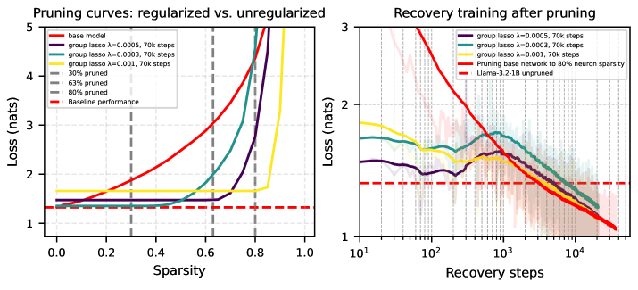
Figure 5: Left: Neuron sparsity vs. loss curve for networks tuned with group lasso regularization with varying $\lambda$ for 70k steps vs. base network. Regularization flattens the sparsity vs. loss curve, at the cost of slightly degrading model performance. Right: after pruning our networks to 30%, 63%, and 80% sparsity for our runs with $\lambda$ of 5e-4, 3e-4, and 1e-3, respectively, we recover performance with additional training. We find that we can recover performance lost during pruning, including in the network that was pruned without first using group-lasso regularization training.

We train networks with the Llama 3 Grattafiori et al. (2024) architecture of varying shape and size. We use a learning rate of 5e-4, sequence length of 1024, and batch size of 64. For distillation, we use Llama-3.1-8B as a teacher with $T=2$. For pruning + recovery, we prune Llama-3.2-1B to varying levels of neuron and residual stream sparsity, shown in Appendix Table˜2. In Appendix Figure˜12 we show learning curves for these three approaches. In Figure˜6, we tentatively find that pruning substantially outperforms training from scratch and distilling a model from scratch on the data-parameter frontier. Given a target narrow network size and a fixed data budget, if one already has access to a general model, it appears to be more efficient to prune that model than it is to perform distillation.

We discuss one last finding: pruning random model components performs about as well as pruning lowest-attribution components Xu et al. . In Appendix Figure˜13, we find that after a moderate number of recovery steps, attribution pruning and random pruning result in the same recovered performance. This result is in line with our earlier discussion of nonlocality, and the empirical findings of Bricken et al. (2023), that monosemantic features are distributed widely across model components. While some studies have found some geometric similarity between functionally similar features Li et al. (2025); Templeton et al. (2024), in our case it does not seem like the relevant features for our task are localized into a set of “Python” vs. “non-Python” neurons, at least that attribution pruning identifies.

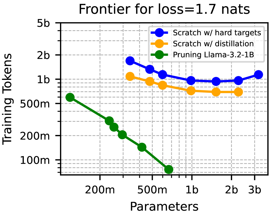
Figure 6: Frontier of network parameters vs. data required to achieve a certain cross-entropy loss on Python documents. For the task of creating a LLM specialized on Python documents, we find that pruning Llama-3.2-1B and then performing recovery training is much more efficient than training LLMs from scratch or distilling LLMs from scratch on the soft targets of Llama-3.2-8B.

6 Related Work

Distillation. Many works have built on the original distillation work of Hinton et al. (2015), seeking to transfer intermediate representations (Romero et al., 2014; Sun et al., 2019) and applying these techniques to language models Jiao et al. (2019); Sanh (2019), often after pruning McCarley et al. (2019); Meta (2024). Relevant to our discussion, Turc et al. (2019) showed that pretraining the student before distillation can substantially improve results.

Pruning. Even early approaches to pruning used second-order methods for pruning weights LeCun et al. (1990); Hassibi and Stork (1993), whereas our “attribution” scores are first-order. When training vision models, Zhou et al. (2016) and Wen et al. (2016) used a group lasso penalty like we do, albeit while training on the full data distribution. Sanh et al. (2020) proposed “movement pruning” to prune weights during transfer learning. A variety of works have applied structured pruning to LLMs Xia et al. (2023); Ma et al. (2023), including Xia et al. (2022) who develop a method for task-specific pruning. Highly relevant to our discussion here is the work of Cloud et al. (2024), who apply “gradient routing” during training to localized network knowledge to different model components, allowing pruning to be used for unlearning.

Task Structure and Learning Dynamics. Several works have lately investigated the relationship between task structure and learning dynamics Ramesh et al. (2023); Okawa et al. (2023); Park et al. (2024); Abbe et al. (2023). Liu et al. (2025) also briefly study a task similar to CMSP to show that hierarchical relationships between tasks cause what they call “domino” learning dynamics.

Machine Unlearning. Many approaches to unlearning have been proposed Cao and Yang (2015); Bourtoule et al. (2019); Yao et al. (2024); Chen and Yang (2023); Gu et al. (2024). Guo et al. (2024) study how applying unlearning fine-tuning to different model components affects unlearning success, inspired by a mechanistic understanding of how knowledge is retrieved in LLMs.

7 Discussion

Limitations: One limitation of our work is that our greedy pruning strategy is quite simple, and we cannot rule out that more sophisticated pruning strategies would be more successful in preserving some skills while unlearning others Li et al. (2022). Also, we did not scale hyperparameters in our LLM experiments, and the performance of each of our models in Section˜5 is likely suboptimal. We also did not evaluate the performance of our models in Section˜4 and Section˜5 outside their narrow distribution $\mathcal{D}_{N}$, and the paper would be more complete if we evaluated how pruning performs not only at achieving good performance on the narrow distribution, but also at unlearning skills outside that distribution.

In this work, we have studied some potential challenges involved in creating narrow AI systems, having to do both with the structure of data and the structures learned internally by neural networks. Underlying this work is a perspective from mechanistic interpretability, that neural networks compute a variety of sparse features Olah et al. (2017), each with a distributed representation Elhage et al. (2022); Bricken et al. (2023); Templeton et al. (2024), and that these features are computed from each other hierarchically in circuits Olah et al. (2020); Marks et al. (2024); Lindsey et al. (2025). First, we found that in order to learn certain complex features, we may have to first train on a broad set of samples which encourage the learning of simpler features. Second, because features are distributed across model components, it is a nontrivial problem to move a set of task-specific features and circuits into a smaller network.

While a neural network’s computation across the whole data distribution may be quite complex, we hope that the computation that networks perform on any particular task will be reducible to something less complex. That less complex computation, whatever it is, might be interpretable as a circuit Marks et al. (2024); Lindsey et al. (2025), or reduce to a simple program Michaud et al. (2024), or, as we studied here, could be instantiated in a much smaller network. However, this hope, and the question of whether it is possible to create narrow-purpose versions of today’s models, probes at a basic question about the nature of the intelligence of these models. If their apparent generality indeed results from their having learned a large, diverse set of crystallized, task-specific circuits, then we ought in principle to be able to create competent, specialized versions of these models by just transferring the relevant task-specific circuits. However, if the intelligence of our models, and intelligence more generally, is better understood as resulting from a single unified algorithm, then the basic prospect of creating narrow AI systems that are as strong as truly general ones could be a challenge.

Appendix A Additional results on CMSP

Here we include some additional results on CMSP. First, in Figure˜7, we provide a supplement to Figure˜2 (bottom right), where here we also include loss curves of a wider network with 361 neurons instead of just 128 neurons. At this width, the single-hidden-layer networks have roughly the same total number of trainable parameters as the networks with two hidden layers of width 128. We observe that the deeper networks still learn faster than the parameter-matched shallow networks.

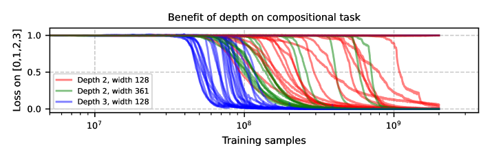
Figure 7: Forty runs of training with different seeds on CMSP dataset ($m=4$, $n=64$, $k=4$) $\mathcal{D}_{\{0\}}\cup\mathcal{D}_{\{1\}}\cup\mathcal{D}_{\{2\}}\cup\mathcal{D}_{\{3\}}\cup\mathcal{D}_{\{0,1,2,3\}}$. 27/40 runs converge with two hidden layers versus 19/40 runs with a single hidden layer with width 128 and 16/40 runs with a single hidden layer and width 361. More obviously however, convergence is faster with two hidden layers. Networks with two hidden layers (depth 3) and width 128 have 25602 total trainable parameters, versus networks with a single hidden layer (depth 2) have 9090 and 25633 parameters for widths 128 and 361 respectively. At width 361, the single-hidden-layer network has roughly the same parameter count as the network with two hidden layers of width 128. This experiment suggests that the beneficial effects of depth are not just due to increased network size, but due to depth.

We also show how ablation scores vary across neurons in our unregularized networks. With the setup in Section˜3.3, we show ablation scores for each neuron for each subtask in Figure˜8 and Figure˜9. We find that there are neurons which have high scores across most subtasks, even subtasks in different “skill trees” ({0,1,2} versus {3,4,5}).

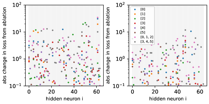
Figure 8: For each hidden neuron in the first hidden layer (left) and the second hidden layer (right) in a CMSP network, we show the ablation score of that neuron for each subtask. For some neurons, ablation scores are high across multiple subtasks, even from separate “skill trees”.

Figure 9: Ablation scores for each subtask and each neuron. This is simply a different way of visualizing the results in Figure˜8.

In Figure˜10 we show sparsity vs accuracy curves from pruning like in Figure˜3 (bottom left), across seeds and network sizes. In our unregularized networks, there is a lot of variation between runs in how entangled the different subtasks are.

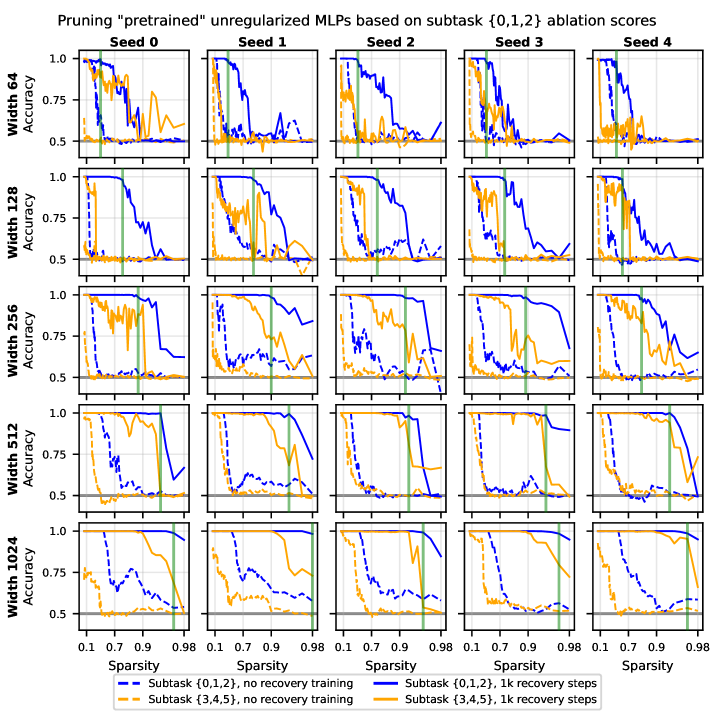
Figure 10: Pruning sparsity vs accuracy curves for pretrained CMSP networks. We train MLPs of varying width and random seed on a CMSP dataset with two skill trees, as in Figure˜3. We prune neurons based on ablation score on subtask {0,1,2}. On some networks, ablating neurons to maximum sparsity while preserving performance on subtask {0,1,2} robustly unlearns subtask {3,4,5}. However, for other networks, the subtasks seem more entangled, and we can recover performance on subtask {3,4,5} even after ablating to the maximum extent we can still recover 98% accuracy on subtask {0,1,2} (green line).

Appendix B Additional results on LLMs

B.1 Additional plots

We also show some additional results with LLMs. In Figure˜11, we show how attribution scores correlate with ablation scores in LLMs. We show results for pruning both neurons and residual stream dimensions.

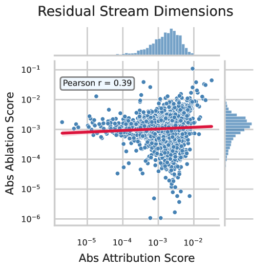
Figure 11: Comparison of ablation vs. attribution scores for Llama-3.2-1B neurons (left) and residual stream dimensions (right), evaluated on a single batch of Python code documents. For each figure, we fully ablate model components and compare the absolute change in loss (Abs Ablation Score, simply called “ablation score” elsewhere in the paper) with the absolute value of the linear estimate of this change computed from model gradients (Abs Attribution Score, called “attribution score” elsewhere). Note that the correlation between the $\log$ of these scores is 0.80 for neurons and 0.05 for residual stream components.

In Figure˜12, we show learning curves across runs when training from scratch on Python documents, when performing distillation, and when performing recovery training after pruning both neurons and residual stream dimensions, to varying target sparsities, of Llama-3.2-1B.

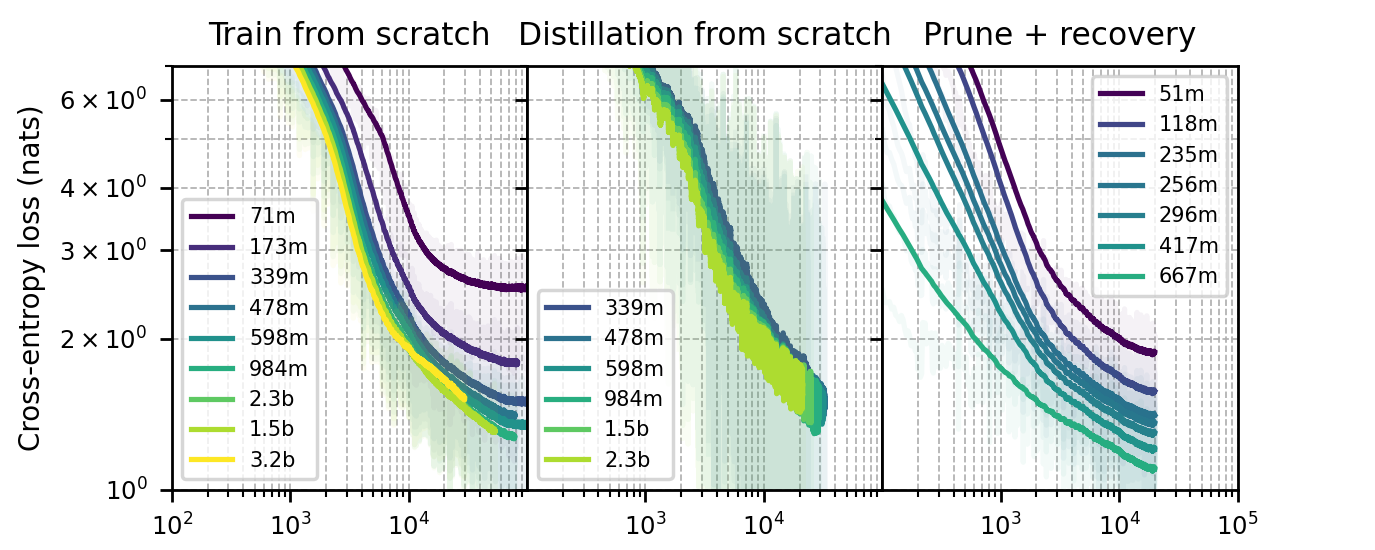
Figure 12: Training curves of LLMs on Python documents when training from scratch (left), training from scratch but with distillation of a larger pretrained LLM (center), and when training pruned pretrained models (right) to recover performance lost during training.

In Figure˜13, we show recovery curves after pruning neurons and residual stream dimensions from Llama-3.2-1B to varying sparsity levels. We find that pruning random components performs roughly as well as pruning components with the lowest attribution scores.

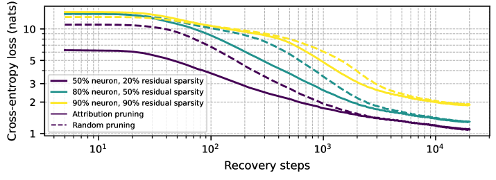
Figure 13: Recovery training curves after pruning neurons and residual stream dimensions, for Llama-3.2-1B on Python code documents. We compare recovery performance when pruning based on attribution scores vs. choosing components randomly. Attribution scores are computed across 1024 documents with a max length of 1024 tokens. We find that pruning with attribution scores is better than pruning random components, however this gap is eventually recovered. For instance, at step 5365 when our run with 50% neuron sparsity and 20% residual sparsity first matches the performance of the original model ($\approx 1.3$ nats), the performance on randomly-pruned model is almost identical at 1.301 nats.

B.2 Additional experimental details

When training networks from scratch and distilling from scratch (Figure˜12 and Figure˜6, we train transformers with the Llama 3 architecture Grattafiori et al. [2024] of varying size, listed in Table˜1.

Table 1: Transformer model configurations explored

Hidden size	#Layers	#Heads	Intermediate size
256	4	4	1,024
512	8	8	2,048
768	12	12	3,072
864	16	16	3,456
1,024	16	16	4,096
1,280	20	20	5,120
1,536	24	24	6,144
1,792	28	28	7,168
2,048	32	32	8,192

When we prune Llama-3.2-1B, we prune neurons and residual stream dimensions with the sparsity combinations shown in Table˜2.

Table 2: Neuron and residual sparsity configurations when using attribution pruning on Llama-3.2-1B.

Neuron sparsity	Residual sparsity
0.50	0.50
0.80	0.50
0.90	0.50
0.95	0.50
0.80	0.80
0.90	0.90

Appendix C Compute estimates

We estimate the compute used for each of our experiments.

For the CMSP training experiments shown in Figure˜2 and Figure˜7, we ran 4 configurations each with 40 different seeds. We ran each job on a GPU, but on a cluster with a variety of different node configurations and GPUs. Jobs generally took between 5-60 minutes to complete, for between 13-160 total hours of GPU time.

For the experiments shown in Figure˜3 and Figure˜10, each run, across 5 choices of seed and 5 choices of width, trained networks on a CMSP task, ran pruning experiments, performed group-lasso training, and pruned again. Each such run took between 5-120 minutes on our cluster with varying GPU configurations, for a total time of 2-50 hours of GPU time.

For our MNIST experiments shown in Figure˜4, we plot a total of 54 points, each of which is averaged over 10 training runs. We estimate that each run took around 2 minutes on our cluster, totaling to around 18 hours of GPU time.

For our LLM experiments, we ran our experiments on A100-80GB nodes, with a single GPU allocated per experiment. When we trained models from scratch on Python documents, we used 9 configurations with job lengths between 1-3 days. For distillation we had 9 configurations with job lengths between 2-3 days, though some jobs failed. For the group lasso training experiments in Figure˜5, we show 3 configurations trained with job lengths of 3 days, and we performed recovery training on these models with a job length of 1 day. We estimate that the total time for these jobs was less than 1600 hours of A100 time, though the full set of experiments we attempted in the work that led to this manuscript could be over 5000 hours.

References

- Ren et al. [2025] ZZ Ren, Zhihong Shao, Junxiao Song, Huajian Xin, Haocheng Wang, Wanjia Zhao, Liyue Zhang, Zhe Fu, Qihao Zhu, Dejian Yang, et al. Deepseek-prover-v2: Advancing formal mathematical reasoning via reinforcement learning for subgoal decomposition. arXiv preprint arXiv:2504.21801, 2025.
- Kassianik et al. [2025] Paul Kassianik, Baturay Saglam, Alexander Chen, Blaine Nelson, Anu Vellore, Massimo Aufiero, Fraser Burch, Dhruv Kedia, Avi Zohary, Sajana Weerawardhena, et al. Llama-3.1-foundationai-securityllm-base-8b technical report. arXiv preprint arXiv:2504.21039, 2025.
- Hui et al. [2024] Binyuan Hui, Jian Yang, Zeyu Cui, Jiaxi Yang, Dayiheng Liu, Lei Zhang, Tianyu Liu, Jiajun Zhang, Bowen Yu, Keming Lu, et al. Qwen2. 5-coder technical report. arXiv preprint arXiv:2409.12186, 2024.
- Bommasani et al. [2021] Rishi Bommasani, Drew A Hudson, Ehsan Adeli, Russ Altman, Simran Arora, Sydney von Arx, Michael S Bernstein, Jeannette Bohg, Antoine Bosselut, Emma Brunskill, et al. On the opportunities and risks of foundation models. arXiv preprint arXiv:2108.07258, 2021.
- Barez et al. [2025] Fazl Barez, Tingchen Fu, Ameya Prabhu, Stephen Casper, Amartya Sanyal, Adel Bibi, Aidan O’Gara, Robert Kirk, Ben Bucknall, Tim Fist, et al. Open problems in machine unlearning for ai safety. arXiv preprint arXiv:2501.04952, 2025.
- Bereska and Gavves [2024] Leonard Bereska and Efstratios Gavves. Mechanistic interpretability for ai safety–a review. arXiv preprint arXiv:2404.14082, 2024.
- Sharkey et al. [2025] Lee Sharkey, Bilal Chughtai, Joshua Batson, Jack Lindsey, Jeff Wu, Lucius Bushnaq, Nicholas Goldowsky-Dill, Stefan Heimersheim, Alejandro Ortega, Joseph Bloom, et al. Open problems in mechanistic interpretability. arXiv preprint arXiv:2501.16496, 2025.
- Tegmark and Omohundro [2023] Max Tegmark and Steve Omohundro. Provably safe systems: the only path to controllable agi. arXiv preprint arXiv:2309.01933, 2023.
- Dalrymple et al. [2024] David Dalrymple, Joar Skalse, Yoshua Bengio, Stuart Russell, Max Tegmark, Sanjit Seshia, Steve Omohundro, Christian Szegedy, Ben Goldhaber, Nora Ammann, et al. Towards guaranteed safe ai: A framework for ensuring robust and reliable ai systems. arXiv preprint arXiv:2405.06624, 2024.
- Tegmark et al. [2025] Max Tegmark, Sören Mindermann, Vanessa Wilfred, and Wan Sie Lee. The singapore consensus on global ai safety research priorities. Conference report, 2025 Singapore Conference on AI: International Scientific Exchange on AI Safety, Singapore, April 2025. URL https://file.go.gov.sg/sg-consensus-ai-safety.pdf.
- Drexler [2019] Eric Drexler, K.\lx@bibnewblockReframing superintelligence: Comprehensive ai services as general intelligence. Future of Humanity Institute Technical Report, 2019. Available at https://www.fhi.ox.ac.uk/wp-content/uploads/Reframing_Superintelligence_FHI-TR-2019-1.1-1.pdf.
- Ramesh et al. [2023] Rahul Ramesh, Ekdeep Singh Lubana, Mikail Khona, Robert P Dick, and Hidenori Tanaka. Compositional capabilities of autoregressive transformers: A study on synthetic, interpretable tasks. arXiv preprint arXiv:2311.12997, 2023.
- Okawa et al. [2023] Maya Okawa, Ekdeep S Lubana, Robert Dick, and Hidenori Tanaka. Compositional abilities emerge multiplicatively: Exploring diffusion models on a synthetic task. Advances in Neural Information Processing Systems, 36:50173–50195, 2023.
- Park et al. [2024] Core Francisco Park, Maya Okawa, Andrew Lee, Ekdeep S Lubana, and Hidenori Tanaka. Emergence of hidden capabilities: Exploring learning dynamics in concept space. Advances in Neural Information Processing Systems, 37:84698–84729, 2024.
- Abbe et al. [2023] Emmanuel Abbe, Enric Boix Adsera, and Theodor Misiakiewicz. Sgd learning on neural networks: leap complexity and saddle-to-saddle dynamics. In The Thirty Sixth Annual Conference on Learning Theory, pages 2552–2623. PMLR, 2023.
- Bricken et al. [2023] Trenton Bricken, Adly Templeton, Joshua Batson, Brian Chen, Adam Jermyn, Tom Conerly, Nick Turner, Cem Anil, Carson Denison, Amanda Askell, Robert Lasenby, Yifan Wu, Shauna Kravec, Nicholas Schiefer, Tim Maxwell, Nicholas Joseph, Zac Hatfield-Dodds, Alex Tamkin, Karina Nguyen, Brayden McLean, Josiah E Burke, Tristan Hume, Shan Carter, Tom Henighan, and Christopher Olah. Towards monosemanticity: Decomposing language models with dictionary learning. Transformer Circuits Thread, 2023. https://transformer-circuits.pub/2023/monosemantic-features/index.html.
- Smolensky [1990] Paul Smolensky. Tensor product variable binding and the representation of symbolic structures in connectionist systems. Artificial intelligence, 46(1-2):159–216, 1990.
- Hinton [1986] Geoffrey E Hinton. Learning distributed representations of concepts. In Proceedings of the Annual Meeting of the Cognitive Science Society, volume 8, 1986.
- Michaud et al. [2023] Eric Michaud, Ziming Liu, Uzay Girit, and Max Tegmark. The quantization model of neural scaling. Advances in Neural Information Processing Systems, 36:28699–28722, 2023.
- Nanda [2023] Neel Nanda. Attribution patching: Activation patching at industrial scale, 2023. URL https://www.neelnanda.io/mechanistic-interpretability/attribution-patching.
- Syed et al. [2023] Aaquib Syed, Can Rager, and Arthur Conmy. Attribution patching outperforms automated circuit discovery. arXiv preprint arXiv:2310.10348, 2023.
- Tibshirani [1996] Robert Tibshirani. Regression shrinkage and selection via the lasso. Journal of the Royal Statistical Society Series B: Statistical Methodology, 58(1):267–288, 1996.
- Yuan and Lin [2006] Ming Yuan and Yi Lin. Model selection and estimation in regression with grouped variables. Journal of the Royal Statistical Society Series B: Statistical Methodology, 68(1):49–67, 2006.
- Wen et al. [2016] Wei Wen, Chunpeng Wu, Yandan Wang, Yiran Chen, and Hai Li. Learning structured sparsity in deep neural networks. Advances in neural information processing systems, 29, 2016.
- Zhou et al. [2016] Hao Zhou, Jose M Alvarez, and Fatih Porikli. Less is more: Towards compact cnns. In Computer Vision–ECCV 2016: 14th European Conference, Amsterdam, The Netherlands, October 11–14, 2016, Proceedings, Part IV 14, pages 662–677. Springer, 2016.
- Hinton et al. [2015] Geoffrey Hinton, Oriol Vinyals, and Jeff Dean. Distilling the knowledge in a neural network. arXiv preprint arXiv:1503.02531, 2015.
- Barak et al. [2022] Boaz Barak, Benjamin Edelman, Surbhi Goel, Sham Kakade, Eran Malach, and Cyril Zhang. Hidden progress in deep learning: Sgd learns parities near the computational limit. Advances in Neural Information Processing Systems, 35:21750–21764, 2022.
- Wei et al. [2022] Jason Wei, Yi Tay, Rishi Bommasani, Colin Raffel, Barret Zoph, Sebastian Borgeaud, Dani Yogatama, Maarten Bosma, Denny Zhou, Donald Metzler, et al. Emergent abilities of large language models. arXiv preprint arXiv:2206.07682, 2022.
- Olsson et al. [2022] Catherine Olsson, Nelson Elhage, Neel Nanda, Nicholas Joseph, Nova DasSarma, Tom Henighan, Ben Mann, Amanda Askell, Yuntao Bai, Anna Chen, Tom Conerly, Dawn Drain, Deep Ganguli, Zac Hatfield-Dodds, Danny Hernandez, Scott Johnston, Andy Jones, Jackson Kernion, Liane Lovitt, Kamal Ndousse, Dario Amodei, Tom Brown, Jack Clark, Jared Kaplan, Sam McCandlish, and Chris Olah. In-context learning and induction heads. Transformer Circuits Thread, 2022. https://transformer-circuits.pub/2022/in-context-learning-and-induction-heads/index.html.
- Nanda et al. [2023] Neel Nanda, Lawrence Chan, Tom Lieberum, Jess Smith, and Jacob Steinhardt. Progress measures for grokking via mechanistic interpretability. arXiv preprint arXiv:2301.05217, 2023.
- Hestness et al. [2017] Joel Hestness, Sharan Narang, Newsha Ardalani, Gregory Diamos, Heewoo Jun, Hassan Kianinejad, Md Mostofa Ali Patwary, Yang Yang, and Yanqi Zhou. Deep learning scaling is predictable, empirically. arXiv preprint arXiv:1712.00409, 2017.
- Kaplan et al. [2020] Jared Kaplan, Sam McCandlish, Tom Henighan, Tom B Brown, Benjamin Chess, Rewon Child, Scott Gray, Alec Radford, Jeffrey Wu, and Dario Amodei. Scaling laws for neural language models. arXiv preprint arXiv:2001.08361, 2020.
- Shoshani and Shamir [2025] Itamar Shoshani and Ohad Shamir. Hardness of learning fixed parities with neural networks. arXiv preprint arXiv:2501.00817, 2025.
- Lin et al. [2017] Henry W Lin, Max Tegmark, and David Rolnick. Why does deep and cheap learning work so well? Journal of Statistical Physics, 168:1223–1247, 2017.
- Olah et al. [2017] Chris Olah, Alexander Mordvintsev, and Ludwig Schubert. Feature visualization. Distill, 2017. doi: 10.23915/distill.00007. https://distill.pub/2017/feature-visualization.
- Elhage et al. [2022] Nelson Elhage, Tristan Hume, Catherine Olsson, Nicholas Schiefer, Tom Henighan, Shauna Kravec, Zac Hatfield-Dodds, Robert Lasenby, Dawn Drain, Carol Chen, Roger Grosse, Sam McCandlish, Jared Kaplan, Dario Amodei, Martin Wattenberg, and Christopher Olah. Toy models of superposition. Transformer Circuits Thread, 2022. https://transformer-circuits.pub/2022/toy_model/index.html.
- Elhage et al. [2021] Nelson Elhage, Neel Nanda, Catherine Olsson, Tom Henighan, Nicholas Joseph, Ben Mann, Amanda Askell, Yuntao Bai, Anna Chen, Tom Conerly, Nova DasSarma, Dawn Drain, Deep Ganguli, Zac Hatfield-Dodds, Danny Hernandez, Andy Jones, Jackson Kernion, Liane Lovitt, Kamal Ndousse, Dario Amodei, Tom Brown, Jack Clark, Jared Kaplan, Sam McCandlish, and Chris Olah. A mathematical framework for transformer circuits. Transformer Circuits Thread, 2021. https://transformer-circuits.pub/2021/framework/index.html.
- Elhage et al. [2023] Nelson Elhage, Robert Lasenby, and Christopher Olah. Privileged bases in the transformer residual stream. Transformer Circuits Thread, page 24, 2023.
- Lecomte et al. [2023] Victor Lecomte, Kushal Thaman, Rylan Schaeffer, Naomi Bashkansky, Trevor Chow, and Sanmi Koyejo. What causes polysemanticity? an alternative origin story of mixed selectivity from incidental causes. arXiv preprint arXiv:2312.03096, 2023.
- Arora et al. [2018] Sanjeev Arora, Yuanzhi Li, Yingyu Liang, Tengyu Ma, and Andrej Risteski. Linear algebraic structure of word senses, with applications to polysemy. Transactions of the Association for Computational Linguistics, 6:483–495, 2018.
- Varma et al. [2023] Vikrant Varma, Rohin Shah, Zachary Kenton, János Kramár, and Ramana Kumar. Explaining grokking through circuit efficiency. arXiv preprint arXiv:2309.02390, 2023.
- LeCun [1998] Yann LeCun. The mnist database of handwritten digits, 1998. URL http://yann.lecun.com/exdb/mnist/.
- Grattafiori et al. [2024] Aaron Grattafiori, Abhimanyu Dubey, Abhinav Jauhri, Abhinav Pandey, Abhishek Kadian, Ahmad Al-Dahle, Aiesha Letman, Akhil Mathur, Alan Schelten, Alex Vaughan, et al. The llama 3 herd of models. arXiv preprint arXiv:2407.21783, 2024.
- [44] Shuyao Xu, Liu Jiayao, Zhenfeng He, Cheng Peng, and Weidi Xu. The surprising effectiveness of randomness in llm pruning. In Sparsity in LLMs (SLLM): Deep Dive into Mixture of Experts, Quantization, Hardware, and Inference.
- Li et al. [2025] Yuxiao Li, Eric J Michaud, David D Baek, Joshua Engels, Xiaoqing Sun, and Max Tegmark. The geometry of concepts: Sparse autoencoder feature structure. Entropy, 27(4):344, 2025.
- Templeton et al. [2024] Adly Templeton, Tom Conerly, Jonathan Marcus, Jack Lindsey, Trenton Bricken, Brian Chen, Adam Pearce, Craig Citro, Emmanuel Ameisen, Andy Jones, Hoagy Cunningham, Nicholas L Turner, Callum McDougall, Monte MacDiarmid, C. Daniel Freeman, Theodore R. Sumers, Edward Rees, Joshua Batson, Adam Jermyn, Shan Carter, Chris Olah, and Tom Henighan. Scaling monosemanticity: Extracting interpretable features from claude 3 sonnet. Transformer Circuits Thread, 2024. URL https://transformer-circuits.pub/2024/scaling-monosemanticity/index.html.
- Romero et al. [2014] Adriana Romero, Nicolas Ballas, Samira Ebrahimi Kahou, Antoine Chassang, Carlo Gatta, and Yoshua Bengio. Fitnets: Hints for thin deep nets. arXiv preprint arXiv:1412.6550, 2014.
- Sun et al. [2019] Siqi Sun, Yu Cheng, Zhe Gan, and Jingjing Liu. Patient knowledge distillation for bert model compression. arXiv preprint arXiv:1908.09355, 2019.
- Jiao et al. [2019] Xiaoqi Jiao, Yichun Yin, Lifeng Shang, Xin Jiang, Xiao Chen, Linlin Li, Fang Wang, and Qun Liu. Tinybert: Distilling bert for natural language understanding. arXiv preprint arXiv:1909.10351, 2019.
- Sanh [2019] V Sanh. Distilbert, a distilled version of bert: smaller, faster, cheaper and lighter. arXiv preprint arXiv:1910.01108, 2019.
- McCarley et al. [2019] JS McCarley, Rishav Chakravarti, and Avirup Sil. Structured pruning of a bert-based question answering model. arXiv preprint arXiv:1910.06360, 2019.
- Meta [2024] AI Meta. Llama 3.2: Revolutionizing edge ai and vision with open, customizable models. Meta AI Blog. Retrieved March 2025, 2024.
- Turc et al. [2019] Iulia Turc, Ming-Wei Chang, Kenton Lee, and Kristina Toutanova. Well-read students learn better: On the importance of pre-training compact models. arXiv preprint arXiv:1908.08962, 2019.
- LeCun et al. [1990] Yann LeCun, John S. Denker, and Sara A. Solla. Optimal brain damage. In David S. Touretzky, editor, Advances in Neural Information Processing Systems 2, pages 598–605. Morgan Kaufmann, 1990. URL https://proceedings.neurips.cc/paper/1989/hash/6c9882bbac1c7093bd25041881277658-Abstract.html.
- Hassibi and Stork [1993] Babak Hassibi and David G. Stork. Second order derivatives for network pruning: Optimal brain surgeon. In Stephen J. Hanson, Jack D. Cowan, and C. Lee Giles, editors, Advances in Neural Information Processing Systems 5, pages 164–171. Morgan Kaufmann, 1993. URL https://proceedings.neurips.cc/paper/1992/hash/647-second-order-derivatives-for-network-pruning-optimal-brain-surgeon.
- Sanh et al. [2020] Victor Sanh, Thomas Wolf, and Alexander Rush. Movement pruning: Adaptive sparsity by fine-tuning. Advances in neural information processing systems, 33:20378–20389, 2020.
- Xia et al. [2023] Mengzhou Xia, Tianyu Gao, Zhiyuan Zeng, and Danqi Chen. Sheared llama: Accelerating language model pre-training via structured pruning. arXiv preprint arXiv:2310.06694, 2023.
- Ma et al. [2023] Xinyin Ma, Gongfan Fang, and Xinchao Wang. Llm-pruner: On the structural pruning of large language models. Advances in neural information processing systems, 36:21702–21720, 2023.
- Xia et al. [2022] Mengzhou Xia, Zexuan Zhong, and Danqi Chen. Structured pruning learns compact and accurate models. arXiv preprint arXiv:2204.00408, 2022.
- Cloud et al. [2024] Alex Cloud, Jacob Goldman-Wetzler, Evžen Wybitul, Joseph Miller, and Alexander Matt Turner. Gradient routing: Masking gradients to localize computation in neural networks. arXiv preprint arXiv:2410.04332, 2024.
- Liu et al. [2025] Ziming Liu, Yizhou Liu, Eric J Michaud, Jeff Gore, and Max Tegmark. Physics of skill learning. arXiv preprint arXiv:2501.12391, 2025.
- Cao and Yang [2015] Yinzhi Cao and Junfeng Yang. Towards making systems forget with machine unlearning. In 2015 IEEE symposium on security and privacy, pages 463–480. IEEE, 2015.
- Bourtoule et al. [2019] Lucas Bourtoule, Varun Chandrasekaran, Christopher A. Choquette-Choo, Hengrui Jia, Adelin Travers, Baiwu Zhang, David Lie, and Nicolas Papernot. Machine unlearning. arXiv preprint arXiv:1912.03817, 2019. doi: 10.48550/arXiv.1912.03817. URL https://arxiv.org/abs/1912.03817.
- Yao et al. [2024] Yuanshun Yao, Xiaojun Xu, and Yang Liu. Large language model unlearning. Advances in Neural Information Processing Systems, 37:105425–105475, 2024.
- Chen and Yang [2023] Jiaao Chen and Diyi Yang. Unlearn what you want to forget: Efficient unlearning for llms. arXiv preprint arXiv:2310.20150, 2023.
- Gu et al. [2024] Kang Gu, Md Rafi Ur Rashid, Najrin Sultana, and Shagufta Mehnaz. Second-order information matters: Revisiting machine unlearning for large language models. arXiv preprint arXiv:2403.10557, 2024.
- Guo et al. [2024] Phillip Guo, Aaquib Syed, Abhay Sheshadri, Aidan Ewart, and Gintare Karolina Dziugaite. Mechanistic unlearning: Robust knowledge unlearning and editing via mechanistic localization, 2024. URL https://arxiv.org/abs/2410.12949.
- Li et al. [2022] Yanyu Li, Pu Zhao, Geng Yuan, Xue Lin, Yanzhi Wang, and Xin Chen. Pruning-as-search: Efficient neural architecture search via channel pruning and structural reparameterization. arXiv preprint arXiv:2206.01198, 2022.
- Olah et al. [2020] Chris Olah, Nick Cammarata, Ludwig Schubert, Gabriel Goh, Michael Petrov, and Shan Carter. Zoom in: An introduction to circuits. Distill, 2020. doi: 10.23915/distill.00024.001. https://distill.pub/2020/circuits/zoom-in.
- Marks et al. [2024] Samuel Marks, Can Rager, Eric J Michaud, Yonatan Belinkov, David Bau, and Aaron Mueller. Sparse feature circuits: Discovering and editing interpretable causal graphs in language models. arXiv preprint arXiv:2403.19647, 2024.
- Lindsey et al. [2025] Jack Lindsey, Wes Gurnee, Emmanuel Ameisen, Brian Chen, Adam Pearce, Nicholas L. Turner, Craig Citro, David Abrahams, Shan Carter, Basil Hosmer, Jonathan Marcus, Michael Sklar, Adly Templeton, Trenton Bricken, Callum McDougall, Hoagy Cunningham, Thomas Henighan, Adam Jermyn, Andy Jones, Andrew Persic, Zhenyi Qi, T. Ben Thompson, Sam Zimmerman, Kelley Rivoire, Thomas Conerly, Chris Olah, and Joshua Batson. On the biology of a large language model. Transformer Circuits Thread, 2025. URL https://transformer-circuits.pub/2025/attribution-graphs/biology.html.
- Michaud et al. [2024] Eric J Michaud, Isaac Liao, Vedang Lad, Ziming Liu, Anish Mudide, Chloe Loughridge, Zifan Carl Guo, Tara Rezaei Kheirkhah, Mateja Vukelić, and Max Tegmark. Opening the ai black box: Distilling machine-learned algorithms into code. Entropy, 26(12):1046, 2024.