Neural Conditional Transport Maps

Abstract

We present a neural framework for learning conditional optimal transport (OT) maps between probability distributions. Our approach introduces a conditioning mechanism capable of processing both categorical and continuous conditioning variables simultaneously. At the core of our method lies a hypernetwork that generates transport layer parameters based on these inputs, creating adaptive mappings that outperform simpler conditioning methods. Comprehensive ablation studies demonstrate the superior performance of our method over baseline configurations. Furthermore, we showcase an application to global sensitivity analysis, offering high performance in computing OT-based sensitivity indices. This work advances the state-of-the-art in conditional optimal transport, enabling broader application of optimal transport principles to complex, high-dimensional domains such as generative modeling and black-box model explainability.

1 Introduction

Optimal transport (OT) is a powerful mathematical framework for comparing and transforming probability distributions, with wide applications across machine learning, computer vision, and scientific computing. OT provides a natural geometry for distribution spaces, offering stronger theoretical guarantees compared to alternative measures (Peyré and Cuturi, 2019). Despite its theoretical appeal, applying OT to high-dimensional, real-world problems has long been constrained by computational limitations. Classical OT methods scale poorly with dimensionality and sample size. Neural approaches have made significant progress in addressing these challenges by approximating transport maps with neural networks (Korotin et al., 2023; Makkuva et al., 2020), enabling efficient computation in high-dimensional spaces.

However, many practical applications require conditional OT maps—transformations that adapt based on auxiliary variables such as labels, time indices, or other parameters. For instance, in climate-economy models, we need to model how distributions of climate variables change based on emissions or policy scenarios. This capability is essential for emulators of computationally intensive models for comprehensive uncertainty quantification. The challenge lies in efficiently computing these conditional transport maps, particularly in data-intensive problems where traditional OT methods become computationally prohibitive.

Global sensitivity analysis (GSA) is another compelling application for conditional OT. GSA quantifies how uncertainty in model outputs can be attributed to different input sources—critical for understanding complex black-box models in climate science, economics, and machine learning (Borgonovo et al., 2024). Recent works leverage OT costs to define GSA indices (Wiesel, 2022; Borgonovo et al., 2024), offering valuable theoretical properties. However, these methods remain constrained by the computational scalability of the underlying OT solvers, limiting their applicability to real-world scientific questions. Efficiently learning conditional transport maps can therefore enable both more robust uncertainty-aware generative models and provide new tools for large-scale black-box model explainability.

In this paper, we introduce a neural framework that efficiently learns conditional OT maps across both categorical and continuous conditioning variables. Our approach leverages a hypernetwork architecture—a neural network that dynamically generates the parameters for transport layers based on conditioning inputs. This mechanism creates highly adaptive mappings that significantly outperform simpler conditioning methods. Our contributions are as follows:

• We extend the Neural Optimal Transport (NOT) framework to conditional settings.

• We introduce a conditioning mechanism capable of simultaneously processing both categorical and continuous variables, using learnable embeddings and positional encoding.

• We propose a hypernetwork-based architecture that generates condition-specific transformation parameters, enabling fundamentally different mappings for each condition value.

• We provide extensive empirical validation across synthetic datasets, climate data, and integrated assessment models, demonstrating superior performance compared to baselines.

• We show an application to global sensitivity analysis, enabling efficient black-box model.

• Upon publication, we will release an open-source implementation of our method and data.

The remainder of this paper is organized as follows. Section 2 reviews related work on traditional and neural OT, and conditioning methods. Section 3 details our conditional neural transport framework, including problem formulation, architecture, and training procedure. Section 4 presents results on benchmark datasets and ablations. Finally, Section 5 discusses limitations and future directions.

2 Background

Optimal Transport has emerged as a powerful mathematical framework across numerous domains. In machine learning, OT has been used for generative modeling (Arjovsky et al., 2017), domain adaptation (Courty et al., 2017), and representation learning (Tolstikhin et al., 2018). In graphics, OT has become fundamental for geometry processing (Solomon et al., 2015), point clouds (Bonneel et al., 2016), noise generation (De Goes et al., 2012), and appearance transfer (Pitié et al., 2007). In computer vision, OT enables image color transfer (Ferradans et al., 2014), shape analysis (Solomon et al., 2016), and texture synthesis (Gao et al., 2019). OT has also been applied to GSA (Borgonovo et al., 2024; Wiesel, 2022), offering sensitivity indices with strong statistical properties.

Neural Optimal Transport approaches began with Wasserstein GANs (Arjovsky et al., 2017), which approximate Wasserstein distances without computing explicit transport maps. Later methods based on Brenier’s theorem (Brenier, 1991) used input convex neural networks (ICNNs) (Makkuva et al., 2020; Amos et al., 2017) to implement Monge maps. However, this formulation is limited to a specific ground cost ($L_{2}^{2})$, and by the existence of Monge maps. Moreover, ICNNs impose severe architectural constraints—requiring non-negative weights, limited activation functions, and specialized initialization—leading to reduced expressivity and optimization difficulties, particularly for conditional problems Korotin et al. (2021). More recently, Korotin et al. introduced neural optimal transport (NOT) (Korotin et al., 2023) and Kernel NOT (Korotin et al., 2022), bypassing these limitations through a minimax formulation supporting general cost functions and stochastic maps. For conditional OT, existing approaches either rely on these restrictive ICNNs (CondOT (Bunne et al., 2022)) or other architectural constraints (Wang et al., 2023). Notably, these methods do not provide standardized benchmarking datasets, hindering systematic comparison across different conditional transport approaches. Our work extends NOT to conditional settings with flexible conditioning mechanisms for both discrete and continuous variables, avoiding the expressivity constraints and training difficulties associated with previous approaches.

Conditioning mechanisms in generative models have evolved from simple concatenation (Ho et al., 2020; Mirza and Osindero, 2014) to more sophisticated approaches including classifier guidance (Dhariwal and Nichol, 2021), normalization (Huang and Belongie, 2017; Perez et al., 2018), attention (Vaswani et al., 2017; Rombach et al., 2022), and hypernetworks (Ha et al., 2017). These methods create a spectrum of expressivity, with hypernetworks offering greater flexibility by dynamically generating parameters for condition-specific transformations. For conditional transport maps, existing approaches like CondOT (Bunne et al., 2022) rely on simple concatenation, limiting their ability to model divergent transport behaviors. Our hypernetwork-based approach enables distinct transformations for different conditions, crucial when conditional distributions require fundamentally different mapping strategies. We provide the first quantitative comparison of conditioning mechanisms in neural optimal transport, showcasing the expressiveness of hypernetworks in this setting.

Figure 1: A diagram of our conditional OT map framework. Our transport network $T$ takes as input samples $x\sim\mathbb{P}$ and transports them to $\mathbb{Q}$, conditioned by $c$. Optionally, $T$ can receive additional noise inputs $z\sim\mathbb{S}$, from a known probability distribution $\mathbb{S}$, introducing stochasticity.

3 Neural Conditional Transport Maps

Conditional OT seeks to learn OT maps that can adapt to different conditions or contexts, an important capability for applications ranging from sensitivity analysis to conditional generative modeling. While classical OT methods struggle with computational scalability or conditioning flexibility, neural approaches offer a promising alternative. In this section, we present our framework for conditional neural OT, which extends the NOT approach of Korotin et al. (2023) with a hypernetwork-based conditioning mechanism. We illustrate our OT maps in Figure 1. We begin by formalizing the conditional OT problem (Section 3.1), then describe our neural architecture that leverages encoder-decoder structures for both transport map $T$ and critic function $f$ (Section 3.2). We introduce our conditioning mechanism that handles both discrete variables and continuous partitions (Section 3.3), present architectural variants including hypernetwork and self-attention approaches (Section 3.4), and detail our training procedure with a custom pretraining strategy (Section 3.5). Implementation details are provided in the supplementary material.

3.1 Problem formulation

Let us consider two probability measures $\mu$ and $\nu$ defined over two Polish spaces, $\mathcal{X}\subset\mathbb{R}^{m}$ and $\mathcal{Y}\subset\mathbb{R}^{n}$, respectively. Let’s also define a lower-semicontinuous cost function $k\colon\mathcal{X}\times\mathcal{Y}\longrightarrow[0,+\infty]$ such that $k(y,y^{\prime})=0$ if and only if $y=y^{\prime}$. The Kantorovich formulation of the OT problem can be stated as follows:

$$K(\mu,\nu)=\inf_{\pi\in\Pi(\mu,\nu)}\int_{\mathcal{X}\times\mathcal{Y}}k(x,y)\,d\pi(x,y),$$ (1)

where $\Pi(\mu,\nu)$ is the set of joint probability measures on $\mathcal{X}\times\mathcal{Y}$ with marginals $\mu$ and $\nu$.

Even though the primal formulation of the OT problem in Equation (1) is easier to interpret, the dual formulation is more useful from a practical perspective, especially using neural networks. First, we introduce the concept of $k$-transform. The $k$-transform $f^{k}$ of a function $f\colon\mathcal{Y}\longrightarrow\mathbb{R}$ is defined as $f^{k}(x)\coloneq\inf_{y\in\mathcal{Y}}\{k(x,y)-f(y)\}$. The dual formulation of the Kantorovich OT problem is then:

$$K(\mu,\nu)=\sup_{f}\left[\int_{\mathcal{X}}f^{k}(x)d\mu(x)+\int_{\mathcal{Y}}f(y)d\nu(y)\right].$$ (2)

For our purposes, the dual problem can be further reformulated as a maximin problem (Korotin et al., 2023). We introduce a third atomless distribution, $\omega$, defined over the Polish space $\mathcal{Z}\subset\mathbb{R}^{s}$. Given a measurable map $T\colon\mathcal{X}\times\mathcal{Z}\longrightarrow\mathcal{Y}$ and its push-forward operator $T\#$, the maximin formulation is:

$$\footnotesize K(\mu,\nu)=\sup_{f}\inf_{T}\mathcal{L}(f,T),$$ (3)

where

$$\mathcal{L}(f,T)=\int_{\mathcal{Y}}f(y)\,d\nu(y)+\int_{\mathcal{X}}\left(k\left(x,T(x,\cdot)\#\omega\right)-\int_{\mathcal{Z}}f(T(x,z))\,d\omega(z)\right)d\mu(x).$$ (4)

We note here that the results in Korotin et al. (2023) can be extended to weak costs, but they are out of the scope of this work.

The conditioned problem. We start from Equation (4) to integrate the conditioning mechanism into the problem formulation. We assume that the condition $c$ belongs to a measure space $\mathcal{C}$. From the theoretical perspective, the extension is straightforward:

$$K(\mu,\nu,c)=\sup_{f}\inf_{T}\mathcal{L}(f,T,c),$$ (5)

where

$$\mathcal{L}(f,T,c)=\int_{\mathcal{Y}}f(y,c)\,d\nu(y)+\int_{\mathcal{X}}\left(k\left(x,T(x,\cdot,c)\#\omega\right)-\int_{\mathcal{Z}}f(T(x,z,c),c)\,d\omega(z)\right)d\mu(x).$$ (6)

Figure 2: Architecture of the conditional networks (transport $T$ and critic $f$). The encoder processes input data ($[x,z]$ for $T$ or $x$ for $f$) through residual blocks to produce latents $h_{L}\in\mathbb{R}^{d}$. We combine discrete variable embeddings $\mathbf{e}_{k}$ with positional encoding of continuous values $PE(p)$ through an MLP to produce the unified conditioning vector $\mathbf{c}\in\mathbb{R}^{d_{c}}$. The conditioning module $\mathcal{C}$ transforms this latent into $h^{\prime}\in\mathbb{R}^{d^{\prime}}$, which the decoder processes into the final output. The noise $z$ is only used in $T$.

3.2 Neural Optimal Transport

Building on the NOT framework of Korotin et al. (2023), we parametrize both the transport map $T$ and critic function $f$ using neural networks. We employ encoder-decoder architectures that enable flexible conditioning in the latent space while supporting various layer types (linear, convolutional, attention) based on the data modality. We illustrate our model design in Figure 2.

Transport & Critic: The transport map $T:\mathcal{X}\times\mathcal{Z}\times\mathcal{C}\rightarrow\mathcal{Y}$ is implemented as a neural network with encoder-decoder structure. For the common case where $\mathcal{X}=\mathcal{Y}=\mathbb{R}^{n}$, the encoder maps $\mathbb{R}^{n+s}$ into $\mathbb{R}^{d}$, a conditioning module transforms $\mathbb{R}^{d}\times\mathcal{C}$ into $\mathbb{R}^{d^{\prime}}$, and the decoder maps $\mathbb{R}^{d^{\prime}}$ into $\mathbb{R}^{n}$. The complete transport map is: $T(x,z,c)=\text{Decoder}_{T}(\text{Conditioning}_{T}(\text{Encoder}_{T}([x,z]),c))$ where $[x,z]\in\mathbb{R}^{n+s}$ denotes the concatenation of input $x$ and noise $z$, $d$ is the latent dimension, and $d^{\prime}$ is the conditioned latent dimension. The critic function $f:\mathcal{Y}\times\mathcal{C}\rightarrow\mathbb{R}$ follows the same structure without noise input: $f(y,c)=\text{Decoder}_{f}(\text{Conditioning}_{f}(\text{Encoder}_{f}(y),c))$

Layer Design: Unlike CondOT (Bunne et al., 2022), which uses ICNNs due to convexity assumptions, our architecture supports more flexible designs. We use residual blocks He et al. (2016) for both $T$ and $f$, along with layer normalization Ba et al. (2016) and orthogonal initialization Saxe et al. (2014). Each block consists of $\text{ResBlock}(h)=h+\alpha\cdot\mathcal{F}(h)$, where $\alpha$ is a learnable scaling parameter and $\mathcal{F}$ represents a composite function that may include normalization, non-linear activations, and appropriate transformations for the data type.

Encoder-Decoder Design: The encoder produces a sequence of hidden states $\{h_{1},h_{2},...,h_{L}\}$ where $h_{L}\in\mathbb{R}^{d}$ is used for conditioning. The decoder takes the conditioned representation and maps to the output space. Both modules can be instantiated with different layer types depending on the data modality: $\text{Encoder}(x)=h_{L}$ where $h_{i}=\text{Layer}_{i}(h_{i-1})$ and $h_{0}=x$. Here, $\text{Layer}_{i}$ can be any differentiable layer. The encoder learns condition-invariant features from the source distribution $\mathbb{P}$, while the decoder applies condition-specific transformations.

Latent Space Conditioning: The conditioning operates on the latent representation $h_{L}\in\mathbb{R}^{d}$ from the encoders. Given a condition $c\in\mathcal{C}$, the conditioning function transforms the latent representation before passing it to the decoder. This design allows the network to learn condition-specific transformations while sharing feature extraction across conditions.

Algorithm 1 Training Neural Conditional Optimal Transport

1: Input: Distributions $\mathbb{P}$, $\mathbb{Q}$, $\mathbb{S}$ accessible by samples; Transport network $T_{\theta}\colon\mathbb{R}^{P}\times\mathbb{R}^{S}\times\mathcal{C}\rightarrow\mathbb{R}^{Q}$; Critic network $f_{\omega}\colon\mathbb{R}^{Q}\times\mathcal{C}\rightarrow\mathbb{R}$;

2:      Cost $\mathcal{L}\colon\mathcal{X}\times\mathcal{Y}\rightarrow\mathbb{R}$; Conditioning distribution $\mathcal{C}$; Maximum steps $N$, Transport iterations per step $K_{T}$

3: Pre-training: Initialize $T_{\theta}$ and $f_{\omega}$ using objectives in Eq. (3)-(7)

4: Output: Learned conditional transport map $T_{\theta}$

5: for $t=1,2,\ldots,N$ do

6:  Sample conditioning $c\sim\mathcal{C}$

7:  Sample batches $Y\sim\mathbb{Q}$, $X\sim\mathbb{P}$; for each $x\in X$ sample $Z_{x}\sim\mathbb{S}$

8:  $\mathcal{L}_{f}\leftarrow\frac{1}{|X|}\sum_{x\in X}\frac{1}{|Z_{x}|}\sum_{z\in Z_{x}}f_{\omega}(T_{\theta}(x,z,c),c)-\frac{1}{|Y|}\sum_{y\in Y}f_{\omega}(y,c)$

9:  Update $\omega$ using $\frac{\partial\mathcal{L}_{f}}{\partial\omega}$ (gradient ascent)

10:  for $k_{T}=1,2,\ldots,K_{T}$ do

11:   Sample conditioning $c\sim\mathcal{C}$

12:   Sample batch $\tilde{X}\sim\mathbb{P}$; for each $x\in\tilde{X}$ sample $\tilde{Z}_{x}\sim\mathbb{S}$

13:   $\mathcal{L}_{T}\leftarrow\frac{1}{|\tilde{X}|}\sum_{x\in\tilde{X}}[\mathcal{L}(x,T_{\theta}(x,\tilde{Z}_{x},c))-\frac{1}{|\tilde{Z}_{x}|}\sum_{z\in\tilde{Z}_{x}}f_{\omega}(T_{\theta}(x,z,c),c)]$

14:   Update $\theta$ using $\frac{\partial\mathcal{L}_{T}}{\partial\theta}$

15:  end for

16: end for

3.3 Conditioning mechanism

Our framework supports conditioning on discrete and continuous variables, with the capability to enable either or both types of conditioning depending on the application. The conditioning module transforms these inputs into a unified representation that modulates the transport map.

For discrete variables (e.g., categorical features with $K$ possible values), we use learnable embeddings. Each variable $k\in\{0,1,...,K-1\}$ is mapped to an embedding $\mathbf{e}_{k}\in\mathbb{R}^{d_{c}}$, where $d_{c}$ is the condition dimensionality, defined as $\mathbf{e}_{k}=\mathcal{E}[k]$ with $\mathcal{E}\in\mathbb{R}^{K\times d_{c}}$. For continuous variables, based on Transformers Vaswani et al. (2017) and Radiance Fields Mildenhall et al. (2020), we use sinusoidal positional encodings to preserve the continuous nature while providing a rich representation:$\text{PE}(p,2i)=\sin\left(\frac{p}{10000^{2i/d}}\right)$, $\text{PE}(p,2i+1)=\cos\left(\frac{p}{10000^{2i/d}}\right)$, where $p$ is the min-max normalized continuous value, $d$ is the encoding dimension, and $i\in\{0,1,...,d/2-1\}$. Additionally, we support other encoding strategies including Fourier features, learned embeddings, or scalar values, allowing flexible adaptation to different problem domains.

Unified Conditioning. The conditioning module flexibly handles discrete variables, continuous variables, or both. When both types are present, their representations are concatenated, then processed to produce the final conditioning vector $\mathbf{c}=\text{MLP}([\mathbf{e}_{\text{discrete}},\text{PE}(p_{\text{continuous}})])$, where $[\cdot,\cdot]$ denotes concatenation and MLP is a multi-layer perceptron with SiLU Ramachandran et al. (2017) activations. The resulting vector $\mathbf{c}\in\mathbb{R}^{d_{c}}$ is used to modulate the transport map in the latent space.

Flexible Configuration. Both discrete and continuous conditioning are optional and can be independently enabled or disabled. The module requires at least one type of conditioning to be active. This flexibility allows our framework to adapt to various application domains—from purely categorical problems to continuous spatiotemporal transport tasks. Unlike CondOT (Bunne et al., 2022), we use different conditioning embeddings for T and f, as this showed better performance.

3.4 Conditioning modules variants

We explored several designs for applying the conditioning $\mathbf{c}\in\mathbb{R}^{d_{c}}$ to modulate the transport map.

Hypernetwork Conditioning The hypernetwork generates the final layer weights and biases of the encoder based on the conditioning. Given the encoder output $\mathbf{h}\in\mathbb{R}^{d}$ and conditioning $\mathbf{c}$, the hypernetwork $\mathcal{H}$ is a shallow MLP that generates parameters: $[\mathbf{W},\mathbf{b}]=\mathcal{H}(\mathbf{c}),\text{where }\mathbf{W}\in\mathbb{R}^{d\times n},\mathbf{b}\in\mathbb{R}^{n}$. The final output is then computed as: $\mathbf{y}=\mathbf{h}\mathbf{W}+\mathbf{b}$. Unlike in feature modulation, generating weights allows fundamentally different transformations per condition, essential for optimal transport where different conditions require distinct mapping strategies, providing the expressiveness of separate networks per condition without its increased computational cost.

Alternative Conditioning Mechanisms We evaluated several conditioning strategies beyond our hypernetwork approach. The simplest baseline is Concatenation, which directly combines feature vectors with the condition. More sophisticated approaches include Cross-Attention (Vaswani et al., 2017), which uses attention mechanisms to modulate features based on conditions, and Feature-wise Linear Modulation (FiLM) (Perez et al., 2018), which applies learnable transformations to features. We also tested normalization-based methods like Adaptive Instance Normalization (Huang and Belongie, 2017) and Conditional Layer Normalization (Su et al., 2021), along with attention-inspired techniques such as Squeeze-and-Excite (Hu et al., 2018) and Feature-wise Affine Normalization (FAN) (Zhou et al., 2021). Although these alternatives showed promise in specific scenarios, our hypernetwork approach consistently demonstrated superior performance across all benchmarks. Notably, our lightweight hypernetwork implementation proved to be computationally efficient both in training time and parameter count, making it a sound choice even for low-budget scenarios. We ablate these components on Section 4 and provide more details in the supplementary material.

3.5 Training Procedure

During training, the transport map $T$ and critic function $f$ must maintain adversarial balance while adapting to diverse conditioning values. This creates optimization challenges. We address them through a two-phase approach: pre-training for stable initialization followed by minimax optimization.

Pre-training: Randomly initialized networks may implement highly non-linear transformations far from identity, leading to unstable optimization. Motivated by this observation, we introduce a lightweight pre-training that establishes favorable initial conditions for both networks. We pre-train $T$ to approximate the identity mapping: $\mathcal{L}_{T}^{\text{pre}}=\mathbb{E}_{x\sim\mathbb{P},z\sim\mathbb{S},c\sim\mathcal{C}}[\|T(x,z,c)-x\|_{2}^{2}]$. This initialization ensures that, early in training, the transport map preserves input structure. Besides, we pre-train $f$ with a multi-objective loss: $\mathcal{L}_{f}^{\text{pre}}=\lambda_{\text{smooth}}\mathcal{L}_{\text{smooth}}+\lambda_{\text{transport}}\mathcal{L}_{\text{transport}}+\lambda_{\text{mag}}\mathcal{L}_{\text{mag}}$. First, the smoothness term prevents sharp discontinuities that lead to gradient explosion during adversarial training:$\mathcal{L}_{\text{smooth}}=\mathbb{E}_{x\sim\mathbb{P},c\sim\mathcal{C}}[\|f(x+\epsilon,c)-f(x,c)\|_{2}^{2}]$ where $\epsilon\sim\mathcal{N}(0,\sigma^{2})$. Second, the transport term maintains the OT objective:$\mathcal{L}_{\text{transport}}=\mathbb{E}_{x\sim\mathbb{P},z\sim\mathbb{S},c\sim\mathcal{C}}[f(T(x,z,c),c)]-\mathbb{E}_{y\sim\mathbb{Q},c\sim\mathcal{C}}[f(y,c)]$. This helps $f$ learn meaningful discrimination between transported and target samples from initialization. Finally, a magnitude control term prevents unbounded growth, enhancing stability:$\mathcal{L}_{\text{mag}}=\mathbb{E}_{y\sim\mathbb{Q},c\sim\mathcal{C}}[(|f(y,c)|-1)^{2}]$.

Optimization: Following pre-training, we employ an alternating training that reflects the minimax structure of optimal transport. We detail our approach in Algorithm 1. Following Korotin et al. (2023), we perform $K_{T}>1$ updates for the transport map per critic update. This asymmetry addresses the imbalance in learning complexity—the transport map must learn condition-dependent transformations while maintaining transport constraints, whereas the critic primarily serves as a measure of transport quality. We find $K_{T}\in\{4,6\}$ provides optimal balance between training stability and efficiency.

Conditions Sampling: The performance of this learning procedure depends on how we sample from the conditioning space $\mathcal{C}$ during training. For discrete variables, we use uniform sampling across all categories. For continuous variables, we employ Beta distribution sampling $\text{Beta}(\alpha,\beta)$ with symmetric parameters ($\alpha=\beta=0.95$), which slightly oversamples values around the min and max values in the training datasets. This strategy prevents underfitting in boundary conditions.

Dataset	Metric	Baseline	+Orth.	+Res	+Norm
Black Hole	KL $\downarrow$	2.333	1.888	2.121	2.144
	Wass. $\downarrow$	0.062	0.047	0.041	0.031
Swiss Roll	KL $\downarrow$	1.081	0.904	0.879	0.813
	Wass. $\downarrow$	0.089	0.052	0.041	0.015
MNIST	MMD $\downarrow$	0.047	0.033	0.027	0.028
	Wass. $\downarrow$	0.042	0.037	0.015	0.011
	FID $\downarrow$	2.378	2.333	2.070	2.075
	Acc. $\uparrow$	82.15	100	100	100

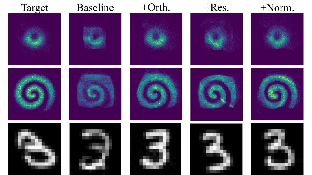
Figure 3: Results of our ablation study comparing different model configurations on an unconditional transport setting. The table presents quantitative metrics, while the right panel shows the visualization.

4 Results

In this section, we present a comprehensive empirical evaluation of our framework. We begin by describing our datasets, which include real scientific data from climate-economy and Integrated Assessment Models. Then, we will present the results of our ablation studies, first examining the impact of simple but effective improvements with respect to the unconditional formulation in Korotin et al. (2023), then systematically evaluating different design choices on the conditional setting, including the use of pretraining and the type of conditioning. Finally, we will show results on the benchmarking tasks and discuss computational aspects of them. Benchmarking data will be released upon publication, more results are provided in the supplementary materials.

4.1 Applications

Climate Economic Impact Distribution Transport

We examine the economic impacts of climate change using the empirical damage function model of Burke et al. (2015). This application requires building an emulator for complex multivariate distributions conditioned on categorical (scenario) and continuous (time) variables.

Problem Formulation. Let $\mathcal{X}\subset\mathbb{R}^{n}$ represent the space of GDP per capita with climate damages across $n=20$ countries. For each country $i$, the impact is quantified through 1000 bootstrap replicates, resulting in a high-dimensional empirical distribution. We define our conditioning space $\mathcal{C}=\mathcal{C}_{\text{ssp}}\times\mathcal{C}_{\text{year}}$, where $\mathcal{C}_{\text{ssp}}=\{0,1,2,3\}$ represents four SSP scenarios (SSP1-1.9, SSP2-4.5, SSP3-7.0, SSP5-8.5) and $\mathcal{C}_{\text{year}}=[2030,2100]$ represents projection years. Our goal is to learn a conditional transport map $T_{\theta}:\mathbb{R}^{n}\times\mathcal{Z}\times\mathcal{C}\rightarrow\mathcal{X}$ that efficiently transforms samples from a reference distribution to match target distributions under different climate scenarios and future years. Thus, we enable efficient sampling of climate impact distributions while preserving their statistical properties, which is needed for appropriate uncertainty quantification.

Global Sensitivity Analysis for Integrated Assessment Models

Our second application focuses on global sensitivity analysis (GSA) for the RICE50+ IAM (Gazzotti, 2022), using the OT-based sensitivity indices presented in Borgonovo et al. (2024).

Problem Formulation. Let $f:\mathcal{C}\subset\mathbb{R}^{3}\rightarrow\mathcal{Y}\subset\mathbb{R}^{58}$ be the RICE50+ model mapping input parameters $\mathbf{C}\in\mathcal{C}$ to the output $\mathbf{Y}\in\mathcal{Y}$. RICE50+  (Gazzotti, 2022) is an IAM with high regional heterogeneity used to assess climate policy benefits and costs. We estimate the sensitivity of the CO₂ emissions for a single region (the output $\mathbf{Y}$) to three inputs $\mathbf{C}$, related to the emissions abatement costs (klogistic), the aversion to inter-country inequality (gamma), and the climate impacts (kw_2), leveraging a subset of the data available in Chiani et al. (2025). Following Borgonovo et al. (2024), the OT-based sensitivity index for variable $C_{i}$ is defined as: $\iota^{K}(\mathbf{Y},C_{i})=\frac{\mathbb{E}_{C_{i}}[K(\mu_{\mathbf{Y}},\mu_{\mathbf{Y}|C_{i}})]}{\mathbb{E}[k(\mathbf{Y},\mathbf{Y}^{\prime})]}$, where $\mu_{\mathbf{Y}}$ is the unconditional output distribution, $\mu_{\mathbf{Y}|C_{i}}$ is the conditional output distribution when variable $C_{i}$ is fixed, and $K$ is the OT cost defined in Eq. (1). Computing these indices traditionally requires solving multiple OT problems for each conditioning variable and partition, which becomes computationally intractable for high-dimensional models or large datasets. Instead, we partition each input space into $M=25$ bins and define our conditioning space $\mathcal{\tilde{C}}=\{0,1,2\}\times[0,1]$, where the first component represents the variable index and the second represents the normalised partition. Our approach learns a single conditional transport map $T_{\theta}:\mathcal{Y}\times\mathcal{Z}\times\mathcal{\tilde{C}}\rightarrow\mathcal{Y}$ parameterised by neural networks.

	Ours	Pretrain	Embed.	Conditioning Type							Continuous Encoding
		False	Shared	Concat	SE	FiLM	FAN	Attn.	CLN	AdaIN	Scalar	Fourier
Comp. cost
Time (s) $\downarrow$	466	451	457	451	554	854	487	921	712	658	464	486
Parameters (k) $\downarrow$	1158	1158	1156	1324	2764	2874	2861	2908	2791	2790	1150	1152
Climate Damages
Wass. $\downarrow$	0.170	0.214	0.265	0.267	0.716	0.974	0.458	0.721	0.691	0.744	0.255	0.172
Wass. $\times$ time $\downarrow$	79.22	96.51	121.1	120.4	396.7	831.8	223.0	664.0	491.9	489.6	118.3	83.59
IAM Data
$\rho$ $\uparrow$	0.942	0.905	0.812	0.305	0.377	0.456	0.388	0.441	0.612	0.682	0.894	0.931
$\rho/\text{time}(\times 100)\uparrow$	0.202	0.200	0.177	0.068	0.068	0.053	0.079	0.048	0.086	0.104	0.193	0.192

Table 1: Ablation study of our conditional transport framework. We report computational cost and accuracy on our datasets. Our final model (leftmost column) uses a hypernetwork with positional encoding and pretraining, without shared embedding. Each other column group represents variations from this configuration. Best results are in green bold, second best are underlined, worst are red.

4.2 Ablation Studies

Unconditional Setting. We first evaluate architectural improvements to the base NOT framework Korotin et al. (2023). We build upon their ReLU-based architectures, incrementally adding orthogonal initialisation, residual connections, and layer normalisation, while preserving identical training configuration and comparable parameter counts across models. In Figure 3, we present results across three datasets. The first two rows show 2D probability distributions, using simple MLPs as our baseline architecture. We measure the KL divergence and Wasserstein loss between targets and transported distributions (from a 2D Uniform prior), using $2^{15}$ samples. The third row showcases a toy convolutional model performing Image-to-Image translation on MNIST (digit 2 to digit 3), evaluated with the MMD distance, Wasserstein loss, FID score, and classification accuracy. In both MLP and convolutional settings, our enhancements yield notable quantitative and qualitative improvements, as shown on the right panel. These architectural enhancements are the foundation of our conditional transport experiments, improving convergence without increasing computational cost.

Conditional Transports. We present our ablation study for our conditional framework in Table 1. We compare our best model configuration, which uses hypernetwork conditioning, pretraining, positional encoding, and separate conditioning embeddings for $T$ and $f$, with variations of that model. For each, we report training time and number of parameters, as well as absolute and cost-adjusted accuracy on two datasets: Climate damages and IAMs. We use the same training setup across datasets and model configurations. Training times are reported for the climate damages dataset. For IAM, we report the Pearson’s correlation $\rho$ between the costs obtained by our model, and those computed with simplex. All experiments are run on a RTX 4070 GPU and an i7-13700H CPU. Using CodeCarbon Lacoste et al. (2019), we measure an electricity consumption of 0.009323 kWh.

Interesting patterns emerge from these results. First, we observe that the conditioning type plays a significant role in training time and accuracy. Our lightweight hypernetwork consistently outperforms simpler alternatives like feature modulation or adaptive normalization. Importantly, we achieve this without a major increase in training cost or trainable parameters. Other complex approaches like cross-attention are suboptimal in accuracy and cost. Concatenation provides the lowest training time, but achieves the worst accuracy on the IAM setting. The encoding performed on the continuous variables also significantly impacts both datasets, with Positional Encoding (our solution) and Fourier features providing the best accuracy, albeit the latter shows less efficiency. This is true for both datasets, where the continuous variable has distinct meanings, suggesting that adequate processing of the raw conditioning plays an important role in expressivity. We also tested whether to share the conditioning embeddings (with hypernetworks) for $T$ and $f$, as proposed in CondOT Bunne et al. (2022). Our results show that separating these embeddings leads to accuracy gains, suggesting that $T$ and $f$ use the condition in distinct ways. Finally, we show that our pretraining algorithm enables higher overall accuracy with no significant added training cost. These results show that adequate, data-driven initialization can improve training dynamics and overall results without efficiency losses.

4.3 Results

Climate Economic Impact Distributions: Figure 4 presents the performance of our model on the climate damages dataset, showing its capability to generate realistic distributions across different climate scenarios. For each SSP scenario, we compare ground truth GDP per capita with climate damages distributions with samples from our conditional transport model over the 2030-2100 time horizon. The results demonstrate our model’s effectiveness at capturing both central tendencies and uncertainty (shaded regions, $90\%$ confidence intervals), specific to each scenario. Our approach learns the distinct patterns across different SSPs: SSP1 shows relatively stable relative impacts with wide uncertainty, while SSP2 exhibits a moderate decline after 2060. The SSP3 scenario shows the most pronounced downward trend, which our model captures accurately despite the smaller uncertainty.

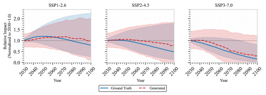
Figure 4: Results of our climate damages model, under different SSP scenarios, on a particular country the dataset. We show the ground truth distribution of damages and samples from our model.

Global Sensitivity Analysis: Figure 5 presents a comparison between our neural transport method and the traditional simplex-based approach for computing OT-based sensitivity indices across three input variables in the RICE50+ model. The first three panels show the transport costs across different partition values (0 to 1) for each variable, with simplex results in blue and our neural method in red. Our neural transport approach closely tracks the simplex cost patterns across all three variables, effectively capturing the complex sensitivity structure of the underlying model. For the klogistic variable (first panel), both methods identify similar regions of high sensitivity, with our neural approach maintaining strong correlation with simplex results. The gamma variable (second) shows more complex sensitivity patterns that our method accurately reproduces, including the pronounced peak near partition value 0.25. For kw_2 (third), both methods detect lower overall sensitivity with consistent patterns across partition values.

The rightmost panel summarizes the average transport costs for each variable. Our neural method preserves the relative importance ordering among variables while maintaining comparable absolute cost values (note that the magnitude of simplex costs may not be comparable with ours). This is critical for GSA applications where accurate ranking of variable importance drives decision-making. Notably, our neural approach achieves this accuracy with higher scalability—requiring a single trained model rather than solving hundreds of individual OT problems. These results demonstrate that our framework enables efficient global sensitivity analysis for complex models, opening new possibilities for comprehensive uncertainty quantification in high-dimensional modeling domains.

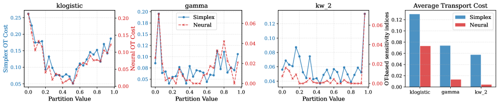
Figure 5: Comparison of simplex and our neural transport across three variables for the IAM dataset. The first three panels show costs across partition values for klogistic, gamma, and kw_2 variables (simplex in blue, neural in red). The rightmost panel shows average costs for each variable.

5 Conclusions

We have presented a neural framework for learning conditional OT maps between probability distributions that extends the NOT framework to handle both categorical and continuous conditioning variables. Our hypernetwork-based architecture generates transport layer parameters dynamically, creating adaptive mappings that significantly outperform simpler conditioning approaches across diverse benchmarks. Experiments on synthetic and real-world datasets demonstrate superior performance compared to existing methods, with ablation studies confirming the value of each architectural component. We have also shown how our approach can effectively be applied to global sensitivity analysis, offering high computational efficiency while maintaining theoretical guarantees.

Limitations and Future Work. Our approach has several limitations: we primarily evaluated residual feedforward networks, not testing recurrent architectures, we have not explored conditioning on complex modalities like CLIP Radford et al. (2021) embeddings or pixel-wise semantic labels, and our hypernetwork approach incurs higher computational costs than simpler alternatives. Besides, our method has been primarily evaluated on climate-related data. Future work could explore multi-modal conditionings, more efficient architectures, applications to image generative models, dynamical systems and causal inference, or connections to diffusion models and normalising flows.

Broader Impacts. Our work could positively impact several fields by enabling more efficient uncertainty quantification and global sensitivity analysis for complex models in climate or economics, potentially leading to better-informed policy decisions. The approach also benefits controlled generative modelling applications and makes advanced optimal transport techniques more accessible to researchers with limited computational resources. However, like most ML techniques, our method could be misused if applied to sensitive domains without appropriate oversight, such as creating more realistic synthetic media. Mitigation strategies include implementing proper access controls, combining sensitivity analysis with domain expertise, and providing educational resources to help practitioners correctly interpret these methods. We believe the benefits outweigh potential risks when appropriate safeguards are implemented.

Appendix A Supplementary Material

We structure this supplementary material as follows:

• In A.1, we provide extensive implementation details for our models, which should enhance reproducibility. Note that we will share our code upon acceptance.

• In A.2, we provide additional implementation guidelines, including some experiments we tested but did not work better than our final configuration. We hope this can provide readers with more information on which pitfalls to avoid and how to quickly adapt our method to their applications.

• In A.3, we provide a theoretical introduction to Global Sensitivity Analysis, and is implementation using Optimal Transport. We build upon this framework for our neural GSA solver.

• In A.4, we provide additional results on our climate-economic damages generative modeling application.

• In A.5, we provide additional results on our Integrated Assessment Model application.

A.1 Implementation Details

Our implementation uses residual blocks for both $T_{\theta}$ and $f_{\omega}$. Each block consists of Layer Normalization [Ba et al., 2016], linear transformations with SiLU activation [Ramachandran et al., 2017], and residual connections with learnable scaling. Residual connections improve gradient flow in deep networks, while the learnable scaling parameter allows the network to control the contribution of the residual path during early training stages. Layer Normalization stabilizes training across a wide range of batch sizes and learning rates, particularly important in our adversarial setting.

We use orthogonal initialization [Saxe et al., 2014] and AdamW [Loshchilov and Hutter, 2019]. Orthogonal initialization preserves gradient norms through deep networks, addressing vanishing and exploding gradient problems typical in transport map training. Gradient norm clipping with threshold $1.0$ prevents gradient explosion during training, especially critical during the adversarial optimization process where critic and transport networks can destabilize each other.

In our experiments, following Korotin et al. [2023], we use the squared Euclidean cost: $k(T(x,z),y)=\|T(x,z)-y\|_{2}^{2}$, but other ground costs could be used. During pre-training, the loss $\mathcal{L}_{f}^{\text{pre}}$ uses equal weights ($\lambda_{\text{smooth}}=\lambda_{\text{transport}}=\lambda_{\text{mag}}=1.0$), with noise $\epsilon\sim\mathcal{N}(0,0.05)$ for the smoothness term. The smoothness term encourages local continuity in the critic, while the magnitude term prevents unbounded growth of critic values. Pre-training runs for 500 steps before transitioning to the alternating optimization of $T_{\theta}$ and $f_{\omega}$ for 5000 epochs, initializing the networks in favorable regions of the parameter space before adversarial training.

In practice, we find $K_{T}=5$ transport iterations per critic update provides good balance between stability and efficiency when computing $\mathcal{L}_{T}$ and $\mathcal{L}_{f}$. This asymmetry accounts for the greater complexity of the transport map’s task compared to the critic function. Across our experiments, we use 4 encoder layers and 8 decoder layers for $T$, and 3 encoder layers and 3 decoder layers for $f$, all with a hidden size of 128 neurons. The transport network requires higher capacity to model complex transformations, while the critic network needs sufficient but not excessive capacity to evaluate transport quality.

For training, we use a learning rate of $2\times 10^{-5}$ for $T$ and $3\times 10^{-5}$ for $f$, both with a weight decay of $0.03$. The slightly higher learning rate for the critic helps it adapt more quickly to changes in the transport map. Conversely, for pretraining, we use the same learning rate and weight decay for both models ($1\times 10^{-4}$ and $0.01$, respectively), as initial alignment does not require the same level of optimization precision.

Our hypernetwork is a 2-layer MLP with SiLU non-linearities and 128 hidden neurons. We use a compressed latent size of 64 neurons for the conditioning. This design provides sufficient capacity to generate the condition-specific weights while maintaining computational efficiency. The hypernetwork approach allows fundamentally different transformations per condition value, essential for optimal transport where different conditions require distinct mapping strategies.

We optimize our hyperparameters using Bayesian optimization through Weights & Biases (WandB), systematically exploring learning rates, weight decay values, initialization, pretraining, regularization, conditioning, and network configurations. Our entire framework is implemented in PyTorch.

A.2 Implementation Guidelines

Through extensive experimentation, we identified several consistent patterns for optimal neural conditional transport implementations. For network architectures, we observed that $T$ should have approximately $1.5-3$ times more trainable parameters than $f$ across all applications. This increased capacity should specifically be allocated through additional hidden layers rather than increasing layer width. Notably, $T$ benefits from an asymmetrical architecture with more decoder layers than encoder layers. This asymmetry aligns with the functional roles: the encoder performs the comparatively simpler task of feature extraction, while the decoder must simultaneously perform the transport mapping and appropriately integrate the conditioning information.

Regarding noise distribution, we found no significant performance difference between uniform and Gaussian priors for the noise variable $z$. However, we selected uniform distributions for our experiments as they provided better training stability during early epochs. For optimization strategies, we tested various learning rate schedulers with inconsistent results across datasets. For simplicity and reproducibility in our ablation studies, we ultimately used constant learning rates without scheduling.

For regularization approaches, standard techniques like dropout did not yield noticeable improvements in our conditional transport setting. In contrast, weight decay significantly enhanced training stability across all experimental configurations. When implementing the hypernetwork component, we discovered that additional or wider layers did not improve performance but instead decreased training stability. Similarly, weight standardization applied to hypernetwork outputs reduced both accuracy and training stability.

Initialization proved important, with orthogonal initialization consistently outperforming alternatives regardless of whether pre-training was employed. For the pre-training phase specifically, our experiments indicate that 500-1000 iterations are sufficient, with diminishing returns observed beyond 500 iterations.

A.3 Global Sensitivity Analysis

Global sensitivity analysis (GSA) studies how the uncertainty in the model output can be apportioned to different sources of uncertainty in the model input. Thus, GSA is crucial when developing and deploying complex models [Saltelli, 2002]. It enables users to understand the parametric components of the model, whether they are inputs like in machine learning models or parametric assumptions like in climate-economy models. OT has been recently introduced in the GSA literature by the works of Wiesel [2022] and Borgonovo et al. [2024]. Here, we present an overview of these OT-based sensitivity indices.

Let’s assume we want to represent some quantities of interest $\mathbf{Y}=(Y_{1},\dots,Y_{k})$ as a function of the inputs $\mathbf{C}=(C_{1},\dots,C_{d})$. We also assume that $\mathbf{C}$ and $\mathbf{Y}$ are random vectors on some probability space $(\Omega,\mathcal{B},\mu)$, and we define with $\mu_{C_{i}}$ and $\mu_{\mathbf{Y}}$ the distributions of $C_{i}$ and $\mathbf{Y}$, respectively. We consider a model defined by the function $\mathbf{f}\colon\mathcal{C}\subset\mathbb{R}^{d}\longrightarrow\mathbb{R}^{k}$. Using the OT cost in Equation (1), we can define the importance of the $i$-th input as:

$$\iota^{K}(\mathbf{Y},C_{i})=\frac{\mathbb{E}_{C_{i}}[K(\mu_{\mathbf{Y}},\mu_{\mathbf{Y}|C_{i}})]}{\mathbb{E}[k(\mathbf{Y},\mathbf{Y}^{\prime})]}.$$ (7)

The rationale behind the index is simple. First, we fix the value of $C_{i}$ at $c_{i}$ and compute the conditional distribution of the output $\mathbf{Y}$ given this information, denoted as $\mu_{\mathbf{Y}|C_{i}=c_{i}}$. Second, we use the metric properties of the OT cost [Peyre and Cuturi, 2019, Chapter 2] to quantify the impact of fixing $C_{i}$ at $c_{i}$. As a third step, the index is computed as the expected value of the OT cost over the domain $\mathcal{C}$. Finally, everything is normalized by the upper bound $\mathbb{E}[k(\mathbf{Y},\mathbf{Y}^{\prime})]$.

The indices in Equation (7) have relevant properties such as zero-independence and max-functionality. Zero-independence reassures us that $\iota^{K}(\mathbf{Y},C_{i})\geq 0$ and $\iota^{K}(\mathbf{Y},C_{i})=0$ if and only if $\mathbf{Y}$ is independent to $C_{i}$, while Max-functionality entails that $\iota^{K}(\mathbf{Y},C_{i})\leq 1$ and $\iota^{K}(\mathbf{Y},C_{i})=1$ if and only if there exists a measurable function $\mathbf{g}$ such that $\mathbf{Y}=\mathbf{g}(C_{i})$.

It is possible to define an estimator for $\iota^{K}(\mathbf{Y},C_{i})$ given a sample of realizations $\{(\mathbf{c}_{j},\mathbf{y}_{j})|j=1,\dots,N\}$. Let $\mathcal{C}_{i}$ denote the support of the input $C_{i}$, partitioned into $M$ subsets, $\mathcal{C}_{i}^{m}$ for $m\in\{1,\dots,M\}$. Under the assumption that $k$ is symmetric, the estimator for the indices is then:

$$\hat{\iota}^{K}(\mathbf{Y},C_{i};N,M)=\frac{N(N-1)}{2M\sum_{j_{1}<j_{2}}k(\mathbf{y}_{j_{1}},\mathbf{y}_{j_{2}})}\sum_{m=1}^{M}K(\mu^{N}_{\mathbf{Y}},\mu^{N}_{\mathbf{Y}|C_{i}\in\mathcal{C}_{i}^{m}}).$$ (8)

The first term in Equation (8) is the U-statistic of the upper bound, and we denote with $\mu^{N}$ the empirical distributions. In the original work, Borgonovo et al. [2024] suggest using well-established and fast solvers like network flow and transportation simplex [Luenberger and Ye, 2021] to compute $K(\mu^{N}_{\mathbf{Y}},\mu^{N}_{\mathbf{Y}|C_{i}\in\mathcal{C}_{i}^{m}})$. The first limitation is that their application requires the computation of the cost matrix, which can be highly memory-intensive for large $N$. Moreover, these solvers do not exploit the potential information in the partition ordering. In our approach, we compute the solution using Equation (5): $K(\mu^{N}_{\mathbf{Y}},\mu^{N}_{\mathbf{Y}|C_{i}\in\mathcal{C}_{i}^{m}})=\sup_{f}\inf_{T}\mathcal{L}(f,T,C_{i}\in\mathcal{C}_{i}^{m})$. Using the conditioned neural solver, we rely on the network structure to share information between partitions and avoid computing and storing the cost matrix.

A.4 Results on Climate Damages

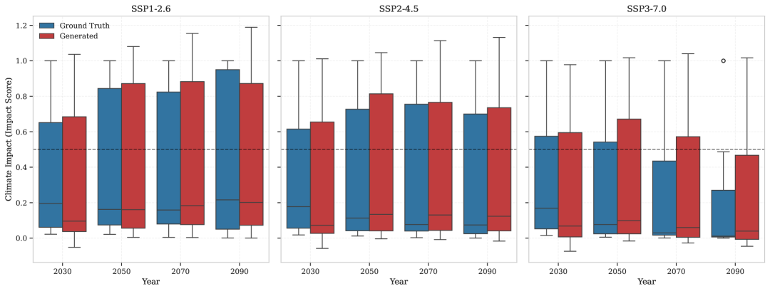
Figure 6: Distribution of ground truth and predictions, across countries, for 3 SSP scenarios and different years. As shown, our model predicts lower values (higher damages) for later years of SSP3, which is consistent with the ground truth distributions. Note that we encode the SSPs using one-hot categorical variables, while years are processed through our positional encoding.

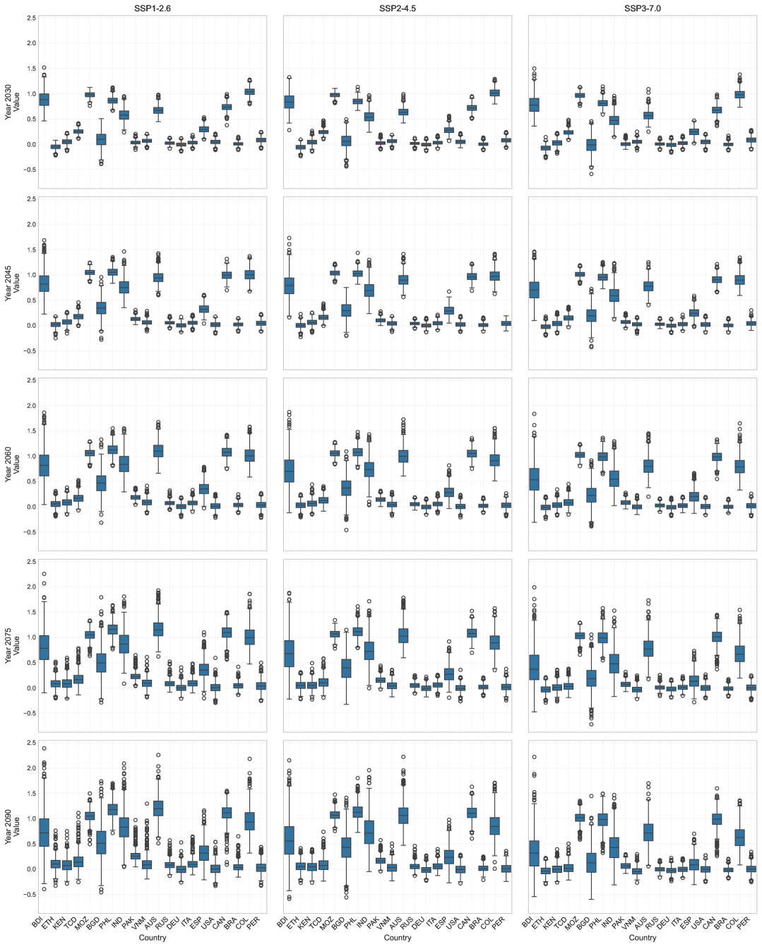
Figure 7: Distribution of predicted evolution of the economies for different countries in our datasets, in different SSP scenarios (columns) and years (rows). Boxplots show the distribution of the predictions, with wider boxplots showing higher uncertainty. For some countries (E.g. Canada or Colombia), the model shows higher uncertainty at the end of the century, while others (eg Italy, Spain, or Germany), both uncertainty and growth are lower, regardless of the SSP.

A.5 Results on Integrated Assessment Models

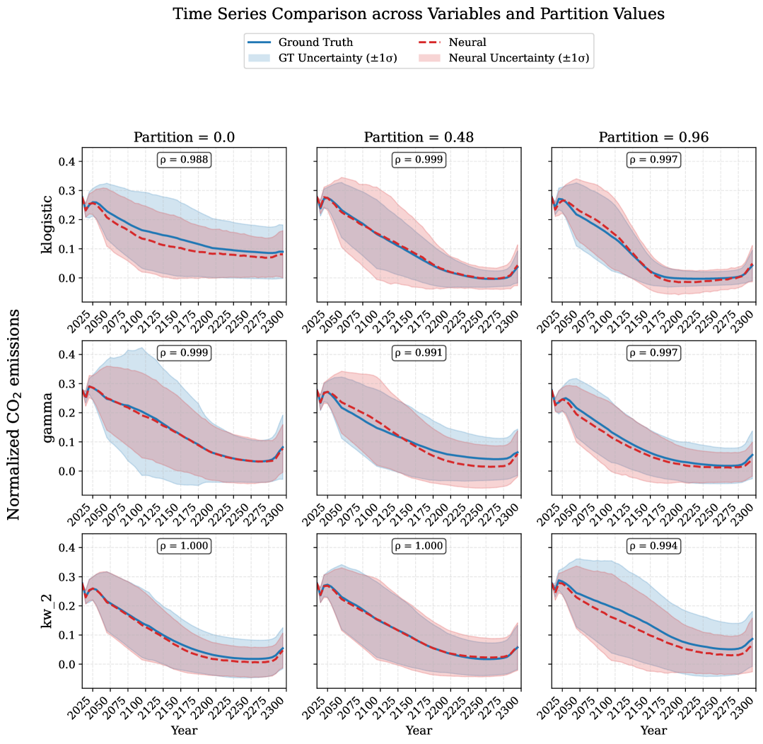
Figure 8: Time series distributions encoded by our model (red) and ground truth counterparts (blue), for different continuous partition values (columns) for the three discrete conditioning variables (rows) in our Integrated Assessment Model dataset. As shown, both the uncertainty and the median values are accurate across combinations of variables. Importantly, the model seems to adequately learn that the distribution is most sensitive to the klogistic value, as shown in our sensitivity analysis section in the paper.

References

- Peyré and Cuturi [2019] Gabriel Peyré and Marco Cuturi. Computational optimal transport. Foundations and Trends in Machine Learning, 11(5-6):355–607, 2019.
- Korotin et al. [2023] Alexander Korotin, Daniil Selikhanovych, and Evgeny Burnaev. Neural Optimal Transport. In The Eleventh International Conference on Learning Representations, March 2023.
- Makkuva et al. [2020] Ashok Makkuva, Amirhossein Taghvaei, Sewoong Oh, and Jason Lee. Optimal transport mapping via input convex neural networks. In Proceedings of the 37th International Conference on Machine Learning, pages 6672–6681. PMLR, 2020.
- Borgonovo et al. [2024] Emanuele Borgonovo, Alessio Figalli, Elmar Plischke, and Giuseppe Savaré. Global sensitivity analysis via optimal transport. Management Science, 2024.
- Wiesel [2022] Johannes CW Wiesel. Measuring association with wasserstein distances. Bernoulli, 28(4):2816–2832, 2022.
- Arjovsky et al. [2017] Martin Arjovsky, Soumith Chintala, and Léon Bottou. Wasserstein generative adversarial networks. In Proceedings of the 34th International Conference on Machine Learning, pages 214–223. PMLR, 2017.
- Courty et al. [2017] Nicolas Courty, Rémi Flamary, Devis Tuia, and Alain Rakotomamonjy. Optimal transport for domain adaptation. IEEE Transactions on Pattern Analysis and Machine Intelligence, 39(9):1853–1865, 2017.
- Tolstikhin et al. [2018] Ilya Tolstikhin, Olivier Bousquet, Sylvain Gelly, and Bernhard Schoelkopf. Wasserstein auto-encoders. In International Conference on Learning Representations, 2018.
- Solomon et al. [2015] Justin Solomon, Fernando De Goes, Gabriel Peyré, Marco Cuturi, Adrian Butscher, Andy Nguyen, Tao Du, and Leonidas Guibas. Convolutional wasserstein distances: Efficient optimal transportation on geometric domains. ACM Transactions on Graphics (TOG), 34(4):1–11, 2015.
- Bonneel et al. [2016] Nicolas Bonneel, Gabriel Peyré, and Marco Cuturi. Wasserstein barycentric coordinates: histogram regression using optimal transport. ACM Transactions on Graphics, 35(4):71, 2016.
- De Goes et al. [2012] Fernando De Goes, Katherine Breeden, Victor Ostromoukhov, and Mathieu Desbrun. Blue noise through optimal transport. ACM Transactions on Graphics, 31(6):171, 2012.
- Pitié et al. [2007] François Pitié, Anil C Kokaram, and Rozenn Dahyot. Automated colour grading using colour distribution transfer. Computer Vision and Image Understanding, 107(1-2):123–137, 2007.
- Ferradans et al. [2014] Sira Ferradans, Nicolas Papadakis, Gabriel Peyré, and Jean-François Aujol. Regularized discrete optimal transport. SIAM Journal on Imaging Sciences, 7(3):1853–1882, 2014.
- Solomon et al. [2016] Justin Solomon, Raif Rustamov, Leonidas Guibas, and Adrian Butscher. Wasserstein propagation for semi-supervised learning. In International Conference on Machine Learning, pages 306–314. PMLR, 2016.
- Gao et al. [2019] Ruihao Gao, Yongxin Xie, Huaxin Xie, Jian Wang, and Alberto Sangiovanni-Vincentelli. Wasserstein gans for texture synthesis. In Computer Vision – ECCV 2018 Workshops, pages 262–278. Springer, 2019.
- Brenier [1991] Yann Brenier. Polar factorization and monotone rearrangement of vector-valued functions. Communications on pure and applied mathematics, 44(4):375–417, 1991.
- Amos et al. [2017] Brandon Amos, Lei Xu, and J. Zico Kolter. Input Convex Neural Networks. In International Conference on Machine Learning, pages 146–155. PMLR, 2017.
- Korotin et al. [2021] Alexander Korotin, Lingxiao Li, Aude Genevay, Justin M Solomon, Alexander Filippov, and Evgeny Burnaev. Do Neural Optimal Transport Solvers Work? A Continuous Wasserstein-2 Benchmark. In Advances in Neural Information Processing Systems, volume 34, pages 14593–14605. Curran Associates, Inc., 2021.
- Korotin et al. [2022] Alexander Korotin, Daniil Selikhanovych, and Evgeny Burnaev. Kernel neural optimal transport. arXiv preprint arXiv:2205.15269, 2022.
- Bunne et al. [2022] Charlotte Bunne, Andreas Krause, and Marco Cuturi. Supervised Training of Conditional Monge Maps. Advances in Neural Information Processing Systems, 35:6859–6872, December 2022.
- Wang et al. [2023] Zheyu Oliver Wang, Ricardo Baptista, Youssef Marzouk, Lars Ruthotto, and Deepanshu Verma. Efficient neural network approaches for conditional optimal transport with applications in bayesian inference. arXiv preprint arXiv:2310.16975, 2023.
- Ho et al. [2020] Jonathan Ho, Ajay Jain, and Pieter Abbeel. Denoising diffusion probabilistic models. Advances in Neural Information Processing Systems, 33:6840–6851, 2020.
- Mirza and Osindero [2014] Mehdi Mirza and Simon Osindero. Conditional generative adversarial nets. arXiv preprint arXiv:1411.1784, 2014.
- Dhariwal and Nichol [2021] Prafulla Dhariwal and Alexander Nichol. Diffusion models beat GANs on image synthesis. Advances in Neural Information Processing Systems, 34:8780–8794, 2021.
- Huang and Belongie [2017] Xun Huang and Serge Belongie. Arbitrary style transfer in real-time with adaptive instance normalization. In Proceedings of the IEEE International Conference on Computer Vision, pages 1501–1510, 2017.
- Perez et al. [2018] Ethan Perez, Florian Strub, Harm de Vries, Vincent Dumoulin, and Aaron Courville. Film: Visual reasoning with a general conditioning layer. In Proceedings of the AAAI Conference on Artificial Intelligence, volume 32, 2018.
- Vaswani et al. [2017] Ashish Vaswani, Noam Shazeer, Niki Parmar, Jakob Uszkoreit, Llion Jones, Aidan N Gomez, Lukasz Kaiser, and Illia Polosukhin. Attention is all you need. In Advances in Neural Information Processing Systems, pages 5998–6008, 2017.
- Rombach et al. [2022] Robin Rombach, Andreas Blattmann, Dominik Lorenz, Patrick Esser, and Björn Ommer. High-resolution image synthesis with latent diffusion models. In Proceedings of the IEEE/CVF Conference on Computer Vision and Pattern Recognition, pages 10684–10695, 2022.
- Ha et al. [2017] David Ha, Andrew Dai, and Quoc V Le. Hypernetworks. arXiv preprint arXiv:1609.09106, 2017.
- He et al. [2016] Kaiming He, Xiangyu Zhang, Shaoqing Ren, and Jian Sun. Deep residual learning for image recognition. In Proceedings of the IEEE Conference on Computer Vision and Pattern Recognition, pages 770–778, 2016.
- Ba et al. [2016] Jimmy Lei Ba, Jamie Ryan Kiros, and Geoffrey E Hinton. Layer normalization. arXiv preprint arXiv:1607.06450, 2016.
- Saxe et al. [2014] Andrew M Saxe, James L McClelland, and Surya Ganguli. Exact solutions to the nonlinear dynamics of learning in deep linear neural networks. In International Conference on Learning Representations, 2014.
- Mildenhall et al. [2020] Ben Mildenhall, Pratul P Srinivasan, Matthew Tancik, Jonathan T Barron, Ravi Ramamoorthi, and Ren Ng. Nerf: Representing scenes as neural radiance fields for view synthesis. In Proceedings of the European Conference on Computer Vision (ECCV), pages 405–421, 2020.
- Ramachandran et al. [2017] Prajit Ramachandran, Barret Zoph, and Quoc V Le. Searching for activation functions. arXiv preprint arXiv:1710.05941, 2017.
- Su et al. [2021] Jianlin Su, Yu Lu, Shengfeng Pan, Ahmed Murtadha, Bo Wen, and Yunfeng Liu. Roformer: Enhanced transformer with rotary position embedding. arXiv preprint arXiv:2104.09864, 2021.
- Hu et al. [2018] Jie Hu, Li Shen, and Gang Sun. Squeeze-and-excitation networks. In Proceedings of the IEEE Conference on Computer Vision and Pattern Recognition, pages 7132–7141, 2018.
- Zhou et al. [2021] Kaiyu Zhou, Yongxin Liu, Yang Song, Xinggang Yan, and Yu Xiang. Feature-wise bias amplification. arXiv preprint arXiv:2107.12320, 2021.
- Burke et al. [2015] Marshall Burke, Solomon M Hsiang, and Edward Miguel. Global non-linear effect of temperature on economic production. Nature, 527(7577):235–239, 2015.
- Gazzotti [2022] Paolo Gazzotti. Rice50+: Dice model at country and regional level. Socio-Environmental Systems Modelling, 4:18038–18038, 2022.
- Chiani et al. [2025] Leonardo Chiani, Emanuele Borgonovo, Elmar Plischke, and Massimo Tavoni. Global sensitivity analysis of integrated assessment models with multivariate outputs. Risk Analysis, 2025.
- Lacoste et al. [2019] Alexandre Lacoste, Alexandra Luccioni, Victor Schmidt, and Thomas Dandres. Quantifying the carbon emissions of machine learning. arXiv preprint arXiv:1910.09700, 2019.
- Radford et al. [2021] Alec Radford, Jong Wook Kim, Chris Hallacy, Aditya Ramesh, Gabriel Goh, Sandhini Agarwal, Girish Sastry, Amanda Askell, Pamela Mishkin, Jack Clark, Gretchen Krueger, and Ilya Sutskever. Learning transferable visual models from natural language supervision. In Marina Meila and Tong Zhang, editors, Proceedings of the 38th International Conference on Machine Learning, volume 139 of Proceedings of Machine Learning Research, pages 8748–8763. PMLR, 2021. URL https://proceedings.mlr.press/v139/radford21a.html.
- Loshchilov and Hutter [2019] Ilya Loshchilov and Frank Hutter. Decoupled weight decay regularization. In International Conference on Learning Representations, 2019.
- Saltelli [2002] Andrea Saltelli. Sensitivity analysis for importance assessment. Risk analysis, 22(3):579–590, 2002.
- Peyre and Cuturi [2019] Gabriel Peyre and Marco Cuturi. Computational optimal transport. Foundations and Trends in Machine Learning, 11(5-6):355–607, 2019.
- Luenberger and Ye [2021] David G. Luenberger and Yinyu Ye. Linear and Nonlinear Programming, volume 228 of International Series in Operations Research & Management Science. Springer International Publishing, Cham, 2021. ISBN 978-3-030-85449-2 978-3-030-85450-8. doi: 10.1007/978-3-030-85450-8.