Robust extrapolation using physics-related activation functions in neural networks for nuclear masses

Abstract

Given the importance of nuclear mass predictions, numerous models have been developed to extrapolate the measured data into unknown regions. While neural networks—the core of modern artificial intelligence—have been recently suggested as powerful methods, showcasing high predictive power in the measured region, their ability to extrapolate remains questionable. This limitation stems from their ‘black box’ nature and large number of parameters entangled with nonlinear functions designed in the context of computer science. In this study, we demonstrate that replacing such nonlinear functions with physics-related functions significantly improves extrapolation performance and provides enhanced understanding of the model mechanism. Using only the information about neutron (N) and proton (Z) numbers without any existing global mass models or knowledge of magic numbers, we developed a highly accurate model that covers light nuclei (N, Z $>$ 0) up to the drip lines. The extrapolation performance was rigorously evaluated using the outermost nuclei in the measurement landscape, and only the data in the inner region was used for training. We present details of the method and model, along with opportunities for future improvements.

Nuclear masses play a critical role in various fields, including not only nuclear physics, but also astrophysics, neutrino studies, nuclear energy, nuclear security, and more [1]. Numerous studies have been extensively done to predict the unknown masses from existing measurements [2, 3, 4, 5, 6]. Recently, the use of neural networks has emerged as a viable method for accurate predictions across fitting data space [7, 8, 9, 10, 11]. Still, the ability to extrapolate beyond the fitting data space remains limited due to the inherent characteristics of neural networks [12, 13, 14, 15, 16]. While the power of (deep) neural networks originates from the large number of parameters entangled with activation functions, this feature can undermine effectiveness outside the training data distribution as they easily become over-parametrized and overfitted to the specific data space [17, 18]. This drawback also gives rise to the ‘black box’ nature of deep neural networks [19, 20].

Many efforts have been made to establish methods that find the true mathematical expression underlying the given data, which will naturally extrapolate well beyond the data [21, 14, 22, 23]. A method called equation learning was suggested for this purpose: it replaces activation functions with scientific functions (e.g., logarithm) that could be components of the underlying expression and uses sparse learning that prunes unimportant parameters [14, 22, 24].

Typical activation functions in computer science tasks are rectified linear unit (ReLU), hyperbolic tangent, and others. They have been empirically proven to give stable and fast training of deep neural networks and high performance on various tasks such as computer vision, natural language processing, and many more [25, 26]. However, because they were chosen for such a purpose in computer science, they are not easily interpretable for physics, and this is exacerbated by the large number of model parameters. These characteristics also contribute to the weakness of deep neural networks in extrapolating predictions beyond their training range. The replacement of the conventional activation functions with functions regularly used in the specific physics task could possibly mitigate this issue and provide better prediction accuracy. Furthermore, the number of parameters should be reduced to alleviate over-parametrization and to achieve a less complex structure. The reduction can be carried out using a method known as sparse learning with the $L_{0}$ regularization [17].

In ideal equation learning, the analytical expression of the neural network can be obtained after extensively pruning the network with replaced activation functions. This idea was demonstrated on “toy model” examples, but few successful applications were performed for complex and high-dimensional physics tasks [14, 22, 27]. In practice, most physics systems might not be represented by a simple equation. Additionally, applying strong regularization to obtain a simple equation does not necessarily yield optimal performance.

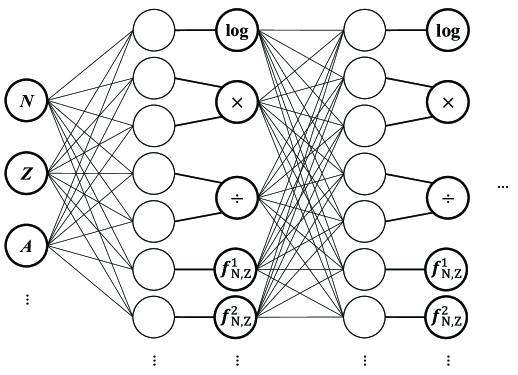
Figure 1: A sketch of the PAF network. Each node of $\div$ or $\times$ takes two nodes as it is operation for two values. $f_{\text{N,Z}}$ represents functions composed of $N$ and $Z$.

In this study, we highlight that using the physics-related activation functions (PAF) with a modest level of sparse learning can lead to an accurate model with highly improved extrapolation—without pursuing a simple analytical equation. We developed a mass model capable of effectively extrapolating beyond existing data, covering nuclei from light isotopes ($N,Z>0$) to the drip lines, with information only on neutron and proton numbers. Fig. 1 shows a sketch of the PAF network structure customized for this study. Its reliability was thoroughly evaluated by allocating a large and less biased portion of experimental data for validation and test. We found that such a network produces highly accurate predictions for both interpolation and extrapolation compared to conventional neural networks and existing global mass models. Throughout the paper, we present details of the network and training method, the performance compared to the conventional neural networks, and a discussion on potential improvements to inspire future advances.

Table 1 summarizes the inputs of the model. Only the information on $N$ and $Z$ was used for inputs; we specifically avoided using any predictions of existing global mass models or magic number information in order to find out if the PAF network could naturally find such characteristics. In addition to the plain integers $N$ and $Z$, odd-even information and various combinations of $N$ and $Z$ were also included as inputs, which may help characterize nuclear mass systematics.

Table 1: Inputs and activation functions of the PAF network. $x$ represent the values propagated through the nodes, and $\%$2 represents the remainder of a division by 2.

Inputs			Activation functions
$N$	$Z$	$A$	$\mathbb{1}$	$\times$	$\div$
$1/N$	$1/Z$	$1/A$	log($x$)	sin($x$)	ReLU
$N\%$2	$Z\%$2		$N^{x}$	$Z^{x}$
$N/Z$	$Z/N$		$x^{N}$	$x^{Z}$
$A^{1/3}$	$A^{2/3}$		$((N-Z)/A)^{x}$

As we are not aware of the specific functions that can capture the underlying physics of the mass system, we tested numerous functions and their combinations. Table 1 shows a list of the functions found to be effective. The feed-forward (densely connected) neural networks already contain the addition ($+$) and subtraction ($-$) in their matrix multiplications with weights and biases. The multiplications ($\times$) and divisions ($\div$) were included to complete the basic arithmetic operations. Commonly used functions in physics, such as sinusoidal and logarithmic functions, were also used. Additionally, we implemented diverse functions composed of $N$ and $Z$, which clearly improved the extrapolation performance. The outputs that may not require any additional operation can pass the identity operation ($\mathbb{1}$). More details are described in Methods.

Sparsity in a neural network can be induced using the $L_{0}$ norm regularization [14, 17]. The $L_{0}$ regularization in the loss function $\mathcal{L}$ penalizes parameters $\boldsymbol{\theta}$ for being non-zero values:

$$\begin{split}\mathcal{L}=-\text{log}(p(\boldsymbol{y}\!\mid\!\boldsymbol{x},\boldsymbol{\theta}))+\lambda\|\boldsymbol{\theta}\|_{0},\end{split}$$ (1)

$$\begin{split}\|\boldsymbol{\theta}\|_{0}=\sum_{i}\mathbbm{I}[\theta_{i}\neq 0],\end{split}$$ (2)

where $-\text{log}(p(\boldsymbol{y}\!\mid\!\boldsymbol{x},\boldsymbol{\theta}))$ is the negative log likelihood with input-output pairs $\boldsymbol{x}$ and $\boldsymbol{y}$, and $\|\boldsymbol{\theta}\|_{0}$ represents the number of non-zero parameters with a weighting factor $\lambda$. This regularization is different from $L_{1}$ or $L_{2}$ as it does not penalize the magnitude of values. The non-differentiable issue of this $L_{0}$ norm was solved by using stochastic gates based on the hard concrete distribution; see ref. [17] for details.

Every 20 epochs during the training, an additional two steps were adopted besides the optimization of the loss function. First, the bound penalty suggested by ref. [22] was used to bound the magnitude of predictions on the extrapolation area in a reasonable range to avoid its drastic changes during the training:

$$\mathcal{L}_{\text{bound}}=\sum_{i}\text{max}(\mid\!f_{\text{NN}}(\boldsymbol{x_{i}};\boldsymbol{\theta})-B_{1}\!\mid\!-B_{2},0),$$ (3)

where the samples $\boldsymbol{x_{i}}$ were randomly selected from the possible extrapolation region ($1,1\leq N,Z\leq 300,200$).

The second step steers the model prediction to softly meet the (algebraic) Garvey-Kelson (GK) relation [28]. Similar to the bound penalty, the loss for the second step was defined as:

$$\begin{split}\mathcal{L}_{\text{GK}}=\sum_{i}\text{max}(\mid\!\Delta(\boldsymbol{x_{i}};N,Z)\!\mid\!-G,0),\end{split}$$ (4)

$$\begin{split}&\Delta(\boldsymbol{x};N,Z)\equiv M_{\text{pred}}(N,Z)+M_{\text{pred}}(N+1,Z-2)\\ &+M_{\text{pred}}(N+2,Z-1)-M_{\text{pred}}(N+2,Z-2)\\ &-M_{\text{pred}}(N,Z-1)-M_{\text{pred}}(N+1,Z),\end{split}$$ (5)

where $\boldsymbol{x_{i}}$ were also randomly selected from the extrapolation region, and $M_{\text{pred}}(N,Z)$ is the model prediction. While $\Delta(\boldsymbol{x};N,Z)$ is equal to zero according to the GK relation, it is not an exact formula [1]. The use of Eq. 4 can avoid forcing the model predictions to strictly follow the relation. See Methods for more details of these two penalties.

Achieving effective extrapolation requires proper validation to ensure model reliability. For machine learning based methods, proper validation necessitates non-biased statistical tests over the landscape both for inter- and extrapolation, rather than using all (or most) existing data for fitting and a small subset for testing. This rigorous validation is critical for nuclear property predictions, as individual isotopes possess distinctive features, making the evaluation dataset prone to bias.

The experimental data in the current study were taken from the atomic mass evaluation (AME2020) [29]. The data was divided into five subsets: the training dataset, two validation datasets for inter- and extrapolation, and two test datasets for inter- and extrapolation. Both validation and test datasets should be prepared to avoid selecting a model biased on the validation datasets during iterative fine-tuning of the model. The extrapolation datasets comprised the outermost nuclei in the nuclear landscape. These include the nuclei with the lowest and highest $Z$ in each isotonic line and those with $N$ in each isotopic line. The training data were sampled exclusively from the interpolation region. Out of the total 2,548 available mass data points, 1,736 were allocated for training, 435 for evaluating interpolation performance, and 377 for evaluating extrapolation performance.

We used the mean squared error for the loss function with the Adam optimizer [30]. The sparsity was kept moderate to obtain high accuracy and extrapolation strength. During the tuning of the network details, such as choices of activation functions, we monitored the root mean square (RMS) errors on the validation datasets as well as the formation of drip lines.

The idea of deep ensembles was implemented to enhance the predictive performance and estimate model uncertainty (see refs. [31, 16]). Sixteen models were trained using the same network and training method with random initialization of model parameters. Aggregating predictions of these models gave a better predictive performance. Still, because of penalty epochs and non-typical regularization, the methodology of deep ensembles might not be strictly followed, possibly resulting in uncertainties that are less well-calibrated. Additional studies on using deep ensembles for such cases are required in the future. Here, we used the standard deviation of the prediction ensembles as an approximate measure of model uncertainties.

Various conventional deep neural networks (DNNs) were also trained to compare with the PAF model. These include densely connected neural networks (DenseNet) with different activation functions and regularizations, as they have the same network structure with the current PAF model. Additionally, we trained convolutional neural networks (ConvNet) to examine the dependence of the results on the network structure. The DenseNet and ConvNet models using ReLU activation achieved the lowest RMS errors and were therefore chosen as representatives. See Methods for more details.

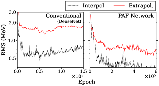
Figure 2: Learning curves of the conventional neural network and PAF network. The curves represent the RMS errors on the validation datasets for interpolation and extrapolation during training. To smooth the curves, an epoch with the lowest RMS for extrapolation is shown for every few thousand epochs.

Table 2: Root mean square errors of different models. It presents the evaluation results on the combined validation and test datasets. Since the Duflo-Zuker, KTUY, WS4, and FRDM were fitted using the different AME version [3, 4, 5, 6], a clear comparison of its inter- and extrapolation performance with the current model is not feasible; therefore, we only present its total RMS error on the AME2020 data.

	RMS ($N,Z\geq 8$) / ($N,Z>0$) (keV)
Model	Interpol.	Extrapol.	Total
PAF Network	207 / 255	308 / 396	258 / 328
DenseNet	494 / 532	1048 / 1173	795 / 889
ConvNet	318 / 409	531 / 658	428 / 539
Duflo-Zuker [3]	-	-	428 / -
KTUY [4]	-	-	733 / 743
WS4 [5]	-	-	295 / -
FRDM [6]	-	-	606 / -

Fig. 2 shows the learning curves of the conventional DNN and PAF models. The error of the PAF model on the validation dataset for extrapolation was clearly reduced over epochs, whereas the DNN could not effectively predict the extrapolation data. The RMS errors of the datasets for each model are shown in Table 2. Among all training epochs, we selected the DNN and PAF models that achieved the lowest RMS errors on the validation dataset for extrapolation. We note that interpolation errors could be further reduced—at the expense of extrapolation performance—by selecting models based on the minimum RMS errors on the interpolation dataset, as is conventionally done. The significantly lower RMS errors of the PAF model indicate that the current method clearly improves the extrapolation ability and could be well-suited for deep learning applications in physics research.

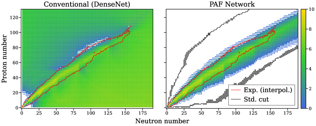
Figure 3: Nuclear landscapes for separation energies. For each nucleus, the lower energy between neutron and proton separation energies is shown, excluding the nuclei with separation energies less than zero, i.e., unbound. The red line shows the experimental data area allocated for interpolation. The outer regions of the landscape for the PAF network were trimmed based on a cutoff using standard deviations (std.) from the model ensembles.

Fig. 3 shows the separation energy predictions of the DNN and PAF models across the nuclear landscape. While both models perform well within the interpolation region, the DNN does not exhibit physically consistent behavior beyond the data range, and does not predict the existence of drip lines. In contrast, the PAF model successfully forms both proton and neutron drip lines. Extended Data Fig. 1 shows closer looks of two nucleon drip lines near the measured unbound regions. Even though most nuclei near the drip lines were excluded from the training dataset, the drip lines formed by the PAF model agree well with the experimental data except for a few discrepancies in the light nuclei region. The landscapes of separation energies for conventional neural networks with different activation functions, structure, regularization, etc. are shown in Extended Data Fig. 2. A different choice of activation functions certainly gave a different landscape, but there were no significant improvements in the extrapolation regions with typical activation functions.

In the PAF model predictions, there are two notable features on the neutron-rich side. First, the effect of shell quenching is predicted at $N=126$, which can be seen in Extended Data Fig. 3. While there is a certain discrepancy between the experimental data and predictions from the PAF for the neutron shell gap near the $N=126$ and $Z=82$, the trend of the data appears to be reasonably reproduced by the predictions. Second, the neutron drip line is closer to the line of stability than other mass models, such as FRDM. This feature emerges for $N>82$, as shown in Extended Data Fig. 4, which will affect the rapid neutron capture process path which approximately follows the contours of neutron separation energies.

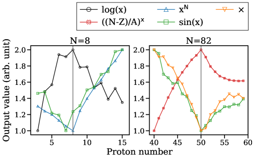
Figure 4: Outputs of the activation functions before the last layer for various $N$ and $Z$. As the output ranges of the activation functions differ, all outputs were normalized to an arbitrary unit for consistent comparison. Gray bars represent magic numbers. Only activation functions exhibiting readily notable features are presented for each subplot.

The PAF network with an additional function $x^{(N-Z)/A}$ or without $N^{x}$ and $Z^{x}$ leads to increased RMS errors, approximately 10 to 20$\%$ for the extrapolation. These results indicate that the nuclear mass system may be more closely associated with terms like $N^{x}$ and $Z^{x}$, or comparable functions of these, rather than $x^{(N-Z)/A}$. The role of each activation function could be interpreted by analyzing its output at each layer. Fig. 4 shows the outputs of each activation function before the last layer as $Z$ varies while $N$ is fixed at magic numbers. Certain functions clearly show inflection points and other discontinuous behaviors at magic numbers, which suggest that these (or comparable) functions might be related to the emergence of magic number effects in nuclear masses. It should be noted that these functions do not solely produce such behaviors, as the outputs from previous layers are accumulated and propagated as the inputs to them.

For evaluation of extrapolation performance, it may seem preferable to use newly updated experimental data from a recent atomic mass evaluation as the validation and test datasets, while using the remaining data for interpolation. However, this approach results in a biased and limited number of samples. We trained the same DNN and PAF networks with the extrapolation datasets composed of newly updated data in AME2020 relative to AME2012. RMS errors ($N,Z>0$) of inter- and extrapolation for ConvNet are 426 and 446 keV, and those for the PAF network were 251 and 273 keV. Clearly, the RMS errors on such data configuration do not fully reflect the poor extrapolation performance of DNNs.

There are several potential ways to enhance the current mass model. Novel inputs and activation functions can be explored, along with variations in the number of layers or nodes. Additionally, alternative ideas for applying the penalties during training may enhance performance—not only through different formulations of boundary or Garvey-Kelson constraints, but also by incorporating more physics to guide predictions in the extrapolation regions.

The effectiveness and utility of physics-related activation functions should be investigated more fully. Tuning the PAF network requires many trials of various sets of activation functions. While a natural approach is to include all possible functions and let the $L_{0}$ regularization prune weights connected to the unnecessary functions, we found that this approach is typically ineffective: including such functions normally degrades the performance. Additionally, increasing the sparsity or making a much smaller network to find a simple formula (as done in equation learning) also degrades the performance, at least in the case of nuclear mass predictions. Improvements in sparse learning could solve these issues, with an easier and better usage of PAF networks. The idea of PAF can also be applied to different types of network structures, such as convolutional neural networks or Transformers [32].

Methods

Architecture

The network architecture was fine-tuned regarding its inputs, the number of layers, activation functions, the number of nodes for each function, and so on. Because of too many possible combinations, we tuned the structure manually without a dedicated tuner.

The integers $N$ and $Z$ provide continuous numerical input that may not capture the appearances of abrupt changes with the addition of a single nucleon. This issue was mitigated by adding values that encode the odd-even information of $N$ and $Z$. Additional inputs, such as the ratios $N/Z$ and $Z/N$, as well as $A^{1/3}$ and $A^{2/3}$, which may roughly represent the radius and surface of the nucleus, were also included. Furthermore, $1/N$, $1/Z$, and $1/A$ were added to introduce features that decrease with increasing nucleon numbers.

Certain activation functions listed in Table 1 can induce unstable training because of the singularities or exponential characteristics. The inputs to some of the functions were taken as absolute values if the function domain should be non-negative. Additional terms suggested by ref. [24] were also introduced: $\text{log}(1+e^{\delta})$, where $\delta$ are learnable parameters, known as relaxation parameters. These terms shift the inputs to avoid the singularities or exponential explosion. For example, the logarithm function became $\text{log}(\mid\!x\!\mid\!+\text{log}(1+e^{\delta}))$.

The model consisted of four layers, with each layer—except the final one—followed by the activation functions. Each activation function was applied to 10 nodes per layer, except for the multiplication ($\times$) and division ($\div$) functions, which were each connected to 20 nodes and returned 10 outputs. Additionally, 10 constant-valued nodes were included and connected only to the subsequent layer, serving a similar role to biases.

Table 3: Hyperparameters for training of the PAF network. ‘lr’ represents the learning rate.

Hyperparameters	Values
lr(weights, biases)	3$\times$10-4
lr($\delta$)	3$\times$10-4
lr(log$\alpha$)	1$\times$10-2
batch size	64
$\lambda$	2.3$\times$10-10
$D_{\text{init}}$	1$\times$10-3
scaling factor for $\text{log}\alpha$	30
epochs	600,000

Sparse Learning

The $L_{0}$ regularization induces zero values of parameters by penalizing parameters for only being non-zero. However, because the $L_{0}$ norm is non-differentiable, more treatments should be incorporated to add it to the loss function. Ref. [17] proposed to use stochastic gates which set weights to zeros, where the parameters $\alpha$ (or $\text{log}\alpha$) of a specific distribution for the gates can then be optimized. Details of this method can be found in ref. [17].

There are several tunable hyperparameters regarding the $L_{0}$ regularization. The main hyperparameters are the weight factor $\lambda$ for $L_{0}$, $D_{\text{init}}$ for initialization of the parameters $\text{log}\alpha$, and the learning rate for $\text{log}\alpha$. $D_{\text{init}}$ controls the percentage of initially pruned parameters. We also found that, at least for the current study, scaling the size of $\text{log}\alpha$ by multiplying a specific factor can greatly affect the sparsity.

To increase the sparsity, higher values of $\lambda$, $D_{\text{init}}$, learning rate, and scaling factor are normally required. The high sparsity will create a simple structure and interpretable equation, as intended by the idea of equation learning. However, we could not achieve high predictive performance when we increased the sparsity to the point where the interpretable equation could be obtained. Instead, we set the parameters for sparse learning as shown in Table 3, aiming for high predictive performance. This regularization pruned approximately 30$\%$ of parameters until the end of the training.

The pruning of weights could reflect the relative importance of certain activation functions, if the weights connected to a certain activation function are pruned more or less frequently. While we found that the weights connected to ReLU were notably more zeroed, this may simply indicate that ReLU is more susceptible to the regularization due to its behavior of outputting zeros for negative inputs.

Penalty Epoch

The absolute value bars in Eq. 3 and 4 are applied to each component of the vector. These terms give penalties if the first arguments of the max function are larger than the second arguments (zero). Therefore, the range of each prediction can be controlled by setting $B_{1}$ and $B_{2}$ in Eq. 3, and $G$ in Eq. 4. Specifically, the bound range of mass excess was set to [$-$0.1, 2] $u$ (atomic mass unit), with $B_{1}$, $B_{2}$=0.95, 1.05 $u$. The range for the deviations from the GK relation, $\Delta(\boldsymbol{x};N,Z)$, was set to [$-$0.5, 0.5] $u$, with $G$=0.5 $u$. While these ranges were tuned to find the optimal setting, the experimentally observed lowest mass excess, $\sim$0.098 $u$ (from ¹¹⁸Sn), was considered to set the lower bound of the bound penalty.

Such penalties were required for achieving reasonable extrapolation in this task, as the implemented activation functions exhibit exponential characteristics that may destabilize predictions in regions far from the training data. For each 20 epochs, the model was trained using the bound penalty (Eq. 3) and the GK penalty (Eq. 4) right before the main optimization for the training dataset. As we found that these two penalty steps at the same epoch induce a more unstable training process, we alternated them at intervals of 10 epochs. The sample size of each penalty epoch was equal to the batch size.

Data Preparation

We used the data from the AME2020 atomic mass evaluation for the current study [29]. The datasets contain five subsets to test the inter- and extrapolation performance: the training dataset, two validation datasets for inter- and extrapolation, and two test datasets for inter- and extrapolation.

Light isotopes with $A\leq 3$, namely, ²H, ³H, and ³He, were considered as interpolation region. In the interpolation region, the data samples were randomly divided for training, validation, and test datasets, except for these light isotopes, as the evaluation can be biased if all of them are allocated in a specific dataset. For this reason, we manually allocated ²H and ³He in the training dataset and ³H in the test dataset.

There are not many isotopes with $N<8$ or $Z<8$ in the training dataset. Randomly splitting the training dataset into many mini-batches may create biased batches that include much less or much more of the light isotopes. Such biased batches can induce unstable training as predicting masses of the light isotopes is more challenging than predicting the heavier ones. For this reason, we randomly included at least one isotope with $N<8$ or $Z<8$ in each batch.

The extrapolation data were set to avoid bias as much as possible, because even neighboring nuclei have distinctive nuclear properties. The extrapolation datasets comprised the outermost nuclei in the nuclear landscape, which gives a reliable evaluation of the extrapolation region. These include the nuclei with the lowest and highest $Z$ in each isotonic line and those with $N$ in each isotopic line, except for $A\leq 3$.

Conventional Neural Networks

The inputs used for the conventional neural networks were identical to those of the PAF model. For the DenseNet, the architecture was designed to be comparable to the PAF model, consisting of four layers with 120 nodes each. The deeper DenseNet shown in Extended Data Fig. 2 was composed of six layers with an increasing number of nodes: 256$\rightarrow$256$\rightarrow$512$\rightarrow$512$\rightarrow$1024$\rightarrow$1. To accommodate the input format required by ConvNet, an additional axis was added to the input. They contained four 1D convolutional layers with increasing channel widths: 1$\rightarrow$128$\rightarrow$256$\rightarrow$512$\rightarrow$512. Sixteen models for each structure were trained to create the model ensembles.

List of Extended Data Figures 1 Experimental mass data and two nucleon drip lines. Each nucleus is labeled as either bound or unbound based on its measured separation energy.

List of Extended Data Figures 2 Same as Fig. 3 with different activation functions, structures, and regularizations of conventional neural networks. Hyper-tangent represents the hyperbolic tangent.

List of Extended Data Figures 3 Neutron shell gaps ($\Delta_{n}$=$\text{S}_{2n}(N,Z)-\text{S}_{2n}(N+2,Z)$) for $N$=8, 20, 28, 50, 82, and 126 as a function of $Z$.

List of Extended Data Figures 4 Two neutron drip lines and nuclei with $1.5<\text{S}_{2n}<2.5$ MeV.

References

- Lunney et al. [2003] D. Lunney, J. M. Pearson, and C. Thibault, Recent trends in the determination of nuclear masses, Rev. Mod. Phys. 75, 1021 (2003).
- Myers and Swiatecki [1974] W. Myers and W. Swiatecki, The nuclear droplet model for arbitrary shapes, Annals of Physics 84, 186 (1974).
- Duflo and Zuker [1995] J. Duflo and A. Zuker, Microscopic mass formulas, Phys. Rev. C 52, R23 (1995).
- Koura et al. [2005] H. Koura, T. Tachibana, M. Uno, and M. Yamada, Nuclidic mass formula on a spherical basis with an improved even-odd term, Progress of Theoretical Physics 113, 305 (2005).
- Wang et al. [2014] N. Wang, M. Liu, X. Wu, and J. Meng, Surface diffuseness correction in global mass formula, Physics Letters B 734, 215 (2014).
- Möller et al. [2016] P. Möller, A. J. Sierk, T. Ichikawa, and H. Sagawa, Nuclear ground-state masses and deformations: FRDM(2012), Atomic Data and Nuclear Data Tables 109, 1 (2016), arXiv:1508.06294 [nucl-th] .
- Utama et al. [2016] R. Utama, J. Piekarewicz, and H. B. Prosper, Nuclear mass predictions for the crustal composition of neutron stars: A bayesian neural network approach, Phys. Rev. C 93, 014311 (2016).
- Niu and Liang [2018] Z. Niu and H. Liang, Nuclear mass predictions based on bayesian neural network approach with pairing and shell effects, Physics Letters B 778, 48 (2018).
- Lovell et al. [2022] A. E. Lovell, A. T. Mohan, T. M. Sprouse, and M. R. Mumpower, Nuclear masses learned from a probabilistic neural network, Phys. Rev. C 106, 014305 (2022).
- Mumpower et al. [2022] M. R. Mumpower, T. M. Sprouse, A. E. Lovell, and A. T. Mohan, Physically interpretable machine learning for nuclear masses, Phys. Rev. C 106, L021301 (2022).
- Boehnlein et al. [2022] A. Boehnlein, M. Diefenthaler, N. Sato, M. Schram, V. Ziegler, C. Fanelli, M. Hjorth-Jensen, T. Horn, M. P. Kuchera, D. Lee, W. Nazarewicz, P. Ostroumov, K. Orginos, A. Poon, X.-N. Wang, A. Scheinker, M. S. Smith, and L.-G. Pang, Colloquium: Machine learning in nuclear physics, Rev. Mod. Phys. 94, 031003 (2022).
- Barnard and Wessels [1992] E. Barnard and L. Wessels, Extrapolation and interpolation in neural network classifiers, IEEE Control Systems Magazine 12, 50 (1992).
- Haley and Soloway [1992] P. Haley and D. Soloway, Extrapolation limitations of multilayer feedforward neural networks, in [Proceedings 1992] IJCNN International Joint Conference on Neural Networks, Vol. 4 (1992) pp. 25–30 vol.4.
- Martius and Lampert [2016] G. Martius and C. H. Lampert, Extrapolation and learning equations (2016), arXiv:1610.02995 [cs.LG] .
- Gal and Smith [2018] Y. Gal and L. Smith, Sufficient conditions for idealised models to have no adversarial examples: a theoretical and empirical study with bayesian neural networks (2018), arXiv:1806.00667 [stat.ML] .
- Kim et al. [2024] C. H. Kim, K. Y. Chae, M. S. Smith, D. W. Bardayan, C. R. Brune, R. J. deBoer, D. Lu, and D. Odell, Probabilistic neural networks for improved analyses with phenomenological -matrix, Phys. Rev. C 110, 054609 (2024).
- Louizos et al. [2018] C. Louizos, M. Welling, and D. P. Kingma, Learning sparse neural networks through regularization (2018), arXiv:1712.01312 [stat.ML] .
- Bejani and Ghatee [2021] M. M. Bejani and M. Ghatee, A systematic review on overfitting control in shallow and deep neural networks, Artificial Intelligence Review 54, 6391 (2021).
- Buhrmester et al. [2021] V. Buhrmester, D. Münch, and M. Arens, Analysis of explainers of black box deep neural networks for computer vision: A survey, Machine Learning and Knowledge Extraction 3, 966 (2021).
- Jospin et al. [2022] L. V. Jospin, H. Laga, F. Boussaid, W. Buntine, and M. Bennamoun, Hands-on bayesian neural networks—a tutorial for deep learning users, IEEE Computational Intelligence Magazine 17, 29 (2022).
- Schmidt and Lipson [2009] M. Schmidt and H. Lipson, Distilling free-form natural laws from experimental data, Science 324, 81 (2009).
- Sahoo et al. [2018] S. Sahoo, C. Lampert, and G. Martius, Learning equations for extrapolation and control, in Proceedings of the 35th International Conference on Machine Learning, Proceedings of Machine Learning Research, Vol. 80, edited by J. Dy and A. Krause (PMLR, 2018) pp. 4442–4450.
- Udrescu and Tegmark [2020] S.-M. Udrescu and M. Tegmark, Ai feynman: A physics-inspired method for symbolic regression, Science Advances 6, eaay2631 (2020).
- Werner et al. [2021] M. Werner, A. Junginger, P. Hennig, and G. Martius, Informed equation learning (2021), arXiv:2105.06331 [cs.LG] .
- Géron [2019] A. Géron, Hands-On Machine Learning with Scikit-Learn, Keras, and TensorFlow: Concepts, Tools, and Techniques to Build Intelligent Systems, 2nd ed. (O’Reilly Media, Inc., 2019).
- Murphy [2022] K. P. Murphy, Probabilistic machine learning: an introduction (MIT press, Cambridge, 2022).
- Kim et al. [2021] S. Kim, P. Y. Lu, S. Mukherjee, M. Gilbert, L. Jing, V. Čeperić, and M. Soljačić, Integration of neural network-based symbolic regression in deep learning for scientific discovery, IEEE Transactions on Neural Networks and Learning Systems 32, 4166 (2021).
- Garvey and Kelson [1966] G. T. Garvey and I. Kelson, New nuclidic mass relationship, Phys. Rev. Lett. 16, 197 (1966).
- Wang et al. [2021] M. Wang, W. Huang, F. Kondev, G. Audi, and S. Naimi, The ame 2020 atomic mass evaluation (ii). tables, graphs and references*, Chinese Physics C 45, 030003 (2021).
- Kingma and Ba [2015] D. P. Kingma and J. Ba, Adam: A method for stochastic optimization, in 3rd International Conference on Learning Representations, ICLR 2015, San Diego, CA, USA, May 7-9, 2015, Conference Track Proceedings, edited by Y. Bengio and Y. LeCun (2015).
- Lakshminarayanan et al. [2017] B. Lakshminarayanan, A. Pritzel, and C. Blundell, Simple and scalable predictive uncertainty estimation using deep ensembles, in Advances in Neural Information Processing Systems, Vol. 30, edited by I. Guyon, U. V. Luxburg, S. Bengio, H. Wallach, R. Fergus, S. Vishwanathan, and R. Garnett (Curran Associates, Inc., 2017).
- Vaswani et al. [2017] A. Vaswani, N. Shazeer, N. Parmar, J. Uszkoreit, L. Jones, A. N. Gomez, L. u. Kaiser, and I. Polosukhin, Attention is all you need, in Advances in Neural Information Processing Systems, Vol. 30, edited by I. Guyon, U. V. Luxburg, S. Bengio, H. Wallach, R. Fergus, S. Vishwanathan, and R. Garnett (Curran Associates, Inc., 2017).