Human-in-the-Loop Adaptive Optimization for Improved Time Series Forecasting

Abstract

Time series forecasting models often produce systematic, predictable errors—even in critical domains such as energy, finance, and healthcare. We introduce a novel post-training adaptive optimization framework that improves forecast accuracy without retraining or architectural changes. Our method automatically applies expressive transformations—optimized via reinforcement learning, contextual bandits, or genetic algorithms—to correct model outputs in a lightweight and model-agnostic way. Theoretically, we prove that affine corrections always reduce the mean squared error; practically, we extend this idea with dynamic action-based optimization. The framework also supports an optional human-in-the-loop component: domain experts can guide corrections using natural language, which is parsed into actions by a language model. Across multiple benchmarks (e.g., electricity, weather, traffic), we observe consistent accuracy gains with minimal computational overhead. Our interactive demo (link) shows the framework’s real-time usability. By combining automated post-hoc refinement with interpretable and extensible mechanisms, our approach offers a powerful new direction for practical forecasting systems.

1 Introduction

Time series forecasting is critical in domains such as finance (Krollner et al.,, 2010), healthcare (Kaushik et al.,, 2020), and energy management (Palma et al.,, 2024), where accurate predictions drive high-stakes decisions. Although modern machine learning models have improved forecasting performance, they still face two persistent limitations: (1) insufficient model expressiveness to capture complex, real-world patterns, and (2) difficulty incorporating domain expertise into predictions. Traditional forecast pipelines (Meisenbacher et al.,, 2022) often rely on rigid architectures and static assumptions, leading to systematic errors that domain experts can easily identify.

However, integrating expert feedback remains challenging: manual corrections are time consuming, and existing methods (Geweke and Whiteman,, 2006; Girard et al.,, 2002) require extensive re-engineering or ensembling techniques (Khashei and Bijari,, 2012). These limitations prevent models from adapting effectively to changing environments.

To address these issues, we propose a flexible, lightweight post-training optimization framework that improves forecasts without re-training the model. Our preliminary theoretical insight suggests the opportunity for such a post hoc correction. Building on this, we extend post-training correction into a broader optimization framework that adaptively adjusts model outputs using approaches such as reinforcement learning, bandits, or genetic algorithms.

Our proposed approach, illustrated in Figure 2 and Figure 2, is scalable, model-agnostic and accessible through an interactive web interface, making it practical for both researchers and practitioners.

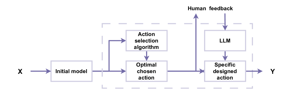
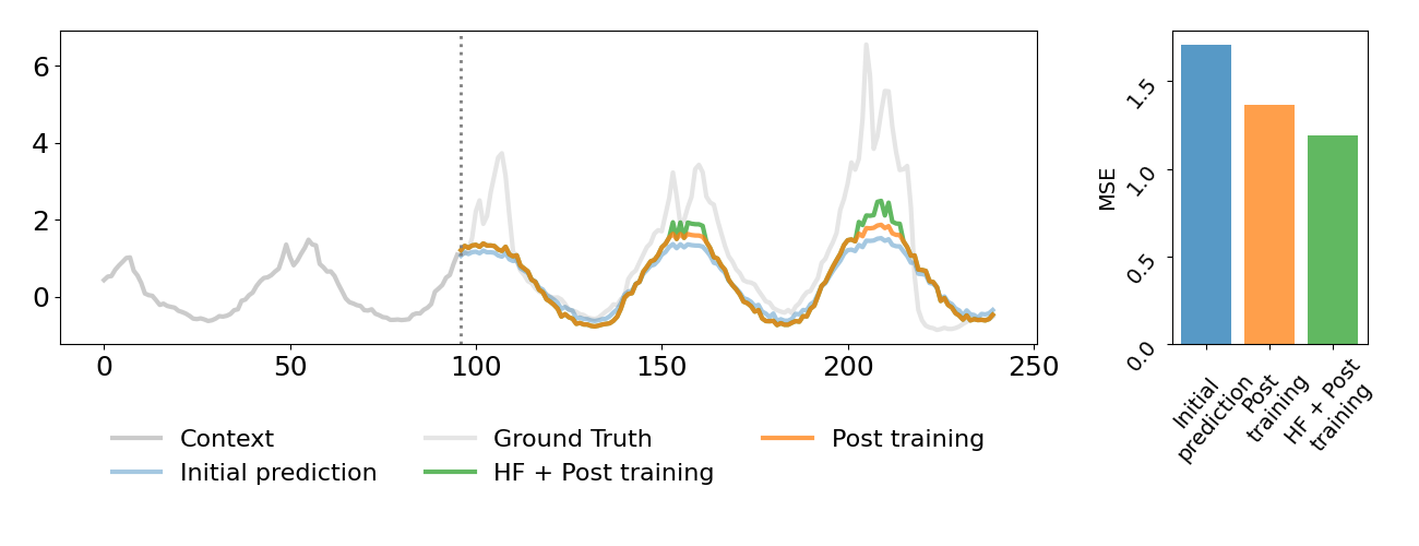
Figure 1: Overview of the forecasting pipeline: the initial model generates predictions from input $X$, which are refined by an action selection mechanism and optionally adjusted using human feedback interpreted by a language model (LLM), yielding the final output $Y$.

Figure 2: (Left) Ground truth, initial prediction, and corrected predictions produced by the proposed forecasting pipeline. The human feedback applied was: “Increase values above a chosen quantile by 10% to 50%.”. (Right) Performance comparison of the different predictions: the base forecast, the automatically corrected output, and the correction incorporating human feedback.

Our novel approach introduces key features that distinguish it from previous work:

1. Adaptive Model Augmentation: Automatically identifies and applies expressive transformations that improve the performance of the forecast, expanding the model function class without architectural changes.

2. Human-in-the-Loop (HITL): Optionally incorporates expert feedback, expressed in natural language, via a language model that maps suggestions to transformations, further refining forecasts interactively.

2 Related Work

Time Series Forecasting Models

Time series forecasting has long been a fundamental task in statistical modeling. Traditional models such as ARIMA (Newbold,, 1983), SARIMA (Korstanje,, 2021), and ETS (Gardner Jr,, 1985) work well for simple linear dynamics, but struggle with non-stationary or highly non-linear signals. Modern deep learning models, including LSTMs (Graves and Graves,, 2012; Lin et al.,, 2023) and Transformers (Liu et al.,, 2023; Ilbert et al.,, 2024; Wu et al.,, 2021), offer improved expressiveness by learning long-range dependencies. Recent zero-shot models such as TimesFM (Das et al.,, 2024), Chronos (Ansari et al.,, 2024), and Lag-LLaMA (Rasul et al.,, 2023) further generalize across tasks via foundation model scaling. Despite these advances, existing models often exhibit systematic forecast errors and lack mechanisms to incorporate expert corrections.

Our work complements existing models by adding a post-training optimization layer that enhances performance without retraining and is compatible with any forecasting architecture.

Post-Training and Human Feedback in Forecasting

Incorporating expert knowledge into forecasting has a long history, from manual tuning and domain-specific feature engineering (Tavenard et al.,, 2020; Zhou,, 2020; Verkade et al.,, 2013; Madadgar et al.,, 2014) to judgmental forecasting methods (Armstrong,, 1986; Bunn and Wright,, 1991; Webby and O’Connor,, 1996). However, such methods are typically manual, hard to scale, and not integrated into learning pipelines. Recent work on human-in-the-loop learning - primarily in NLP (Liu et al., 2024a, ) - has explored expert-guided model refinement. In time series, systems such as DelphAI (Kupferschmidt et al.,, 2022) allow manual modification of model outputs and (Arvan et al.,, 2019) provide a comprehensive review of human input in forecasting.

Our approach advances this line of work in two key ways. First, it enables automatic post-training corrections via adaptive optimization using reinforcement learning, bandits, or genetic algorithms. Secondly, it optionally incorporates expert feedback through natural language, automatically translated into optimization actions by a large-language model (LLM). Unlike methods such as TimeHF (Qi et al.,, 2025), which require fine-tuning large models, our solution is model-agnostic, efficient and applies corrections at inference time.

3 Methodology

We present a general framework to enhance time series forecasts through post-training optimization. The approach operates on top of any forecasting model, applying lightweight corrections that do not require model retraining. It combines two key components: (1) automated prediction augmentation via dynamic optimization, and (2) optional human-in-the-loop feedback. This section first motivates the core theoretical idea and then outlines the full system.

3.1 Theoretical Motivation for Post-Training Correction

Machine learning models, especially in forecasting, often exhibit systematic biases in their predictions. These biases can be reduced after training by applying simple affine transformations to the output—without modifying the model’s parameters.

Let $Y_{\text{pred}}\in\mathbb{R}$ denote the model’s prediction (e.g., for a single time step). The goal is to find optimal scaling and shifting parameters $a^{*},b^{*}$ such that:

$$Y_{\text{corrected}}=a^{*}Y_{\text{pred}}+b^{*}$$

These parameters can be computed using statistics from a validation set:

$$a^{*}=\frac{\text{Cov}(Y_{\text{true}},Y_{\text{pred}})}{\text{Var}(Y_{\text{pred}})},\quad b^{*}=\mathbb{E}[Y_{\text{true}}]-a^{*}\mathbb{E}[Y_{\text{pred}}]$$

Theorem 1 (Affine Correction Reduces MSE)

The affine correction above yields a lower or equal mean squared error (MSE) on the validation set:

$$R_{\text{before}}-R_{\text{after}}=\left(\sqrt{\text{Var}(Y_{\text{pred}})}-\frac{\text{Cov}(Y_{\text{true}},Y_{\text{pred}})}{\sqrt{\text{Var}(Y_{\text{pred}})}}\right)^{2}\geq 0$$

This guarantee holds as long as the validation and test data are drawn from the same distribution. In practice, such post-hoc corrections are both effective and efficient. However, for more complex time series (e.g., multi-step forecasting), static affine transformations may be insufficient. We therefore extend this idea to richer, dynamic correction mechanisms—optimized using reinforcement learning, contextual bandits, or genetic algorithms (see Section 3.3).

Figure 3: Illustration of the effect of affine post-training correction on ridge regression forecasts. The model is trained on a synthetic linear target. Results shown for $100$ samples, $100$ validation points, and $10{,}000$ test points.

3.2 Forecasting Model Setup

Our framework operates on top of any time series forecasting model—traditional (e.g., ARIMA, Prophet), deep learning-based (e.g., LSTM, Transformer), or foundation-level (e.g., TimesFM, Chronos). We assume access to the model’s predictions and apply post-training transformations to improve accuracy.

Let the input be a multivariate time series $\{\mathbf{x}_{1},\dots,\mathbf{x}_{T}\}$ with $\mathbf{x}_{t}\in\mathbb{R}^{d}$. The base model generates forecasts $\{\hat{\mathbf{y}}_{T+1},\dots,\hat{\mathbf{y}}_{T+H}\}$, where $H$ is the forecast horizon.

3.3 Post-Training Optimization via Action Space

To refine model predictions, we define a set of post-training transformations, or actions, each parameterized continuously. These actions are dynamically selected and tuned to minimize validation error.

• Scale Amplitude: Multiplies the full prediction series.

• Piecewise Scaling: Modifies high or low quantiles selectively.

• Linear Trend: Adds a slope or intercept term.

• Min/Max Adjustment: Boosts extrema to match observed dynamics.

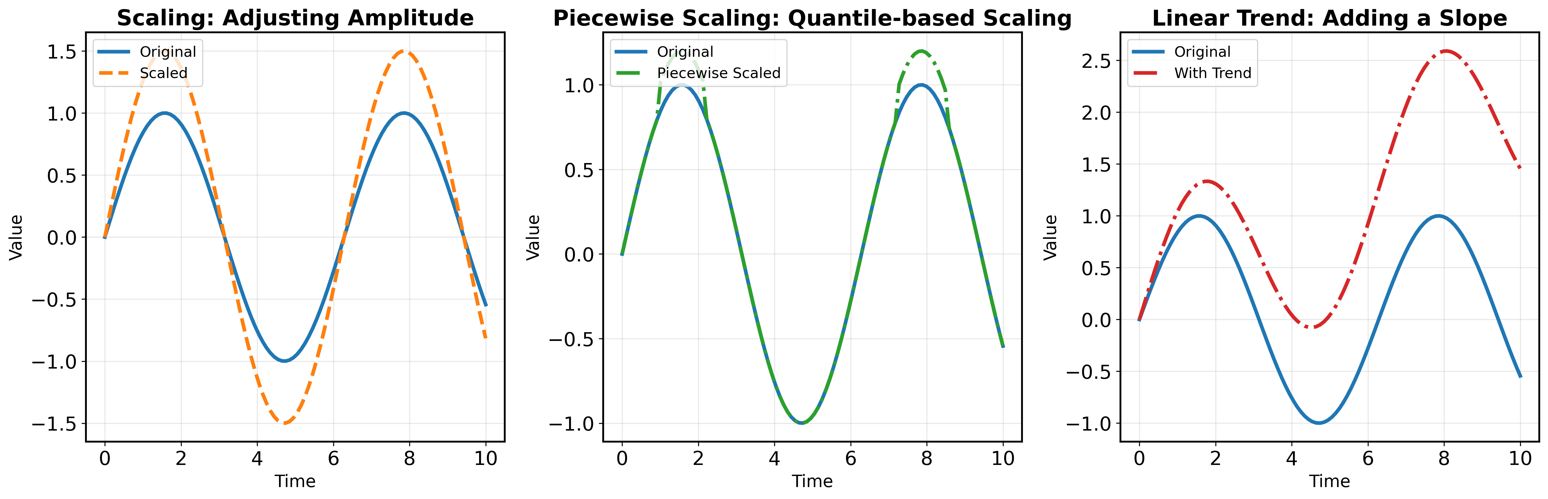
Figure 4: Examples of learned post-training actions. Each transformation operates on the model’s forecast to reduce prediction error. Full action definitions are in Appendix 6.1.

These interpretable actions form a flexible augmentation layer. They can be optimized efficiently and extended to task-specific needs, as discussed in later sections.

3.3.1 Optimizing Actions and Parameters

We frame the post-training refinement process as a joint optimization over a discrete set of actions and their associated continuous parameters. Discrete actions (e.g., scaling, shifting, trend) define transformation types, while parameters control their magnitude. The goal is to select and tune the best combination to minimize validation loss.

Input: Forecasting model $\mathcal{M}$, action space $\mathcal{A}$, validation data $D$

Output: Augmented model $\mathcal{M}_{\text{opt}}$, refined prediction $\hat{\mathbf{y}}$

1

2Generate base predictions $\hat{\mathbf{y}}=\mathcal{M}(D)$

3 Define objective $\mathcal{L}$ (e.g., MSE) on validation set

4 for each iteration do

5    Select candidate action(s) from $\mathcal{A}$

6    Optimize associated parameters (e.g., line search)

7    Apply transformation(s) to $\hat{\mathbf{y}}$

8    Evaluate $\mathcal{L}$ and update strategy

Return best transformation sequence

Algorithm 1 Forecast Augmentation via Post-Training Optimization

3.3.2 Dynamic Optimization Strategies

We explore several strategies to solve this search problem efficiently:

• Random search: For each discrete action, we randomly generate several sets of continuous parameters. We then evaluate these and keep the set that gives the best performance for that action.

• Bandit Algorithms (SH-HPO): (Karnin et al.,, 2013) Each action is a bandit arm; its parameters are optimized independently (e.g., via line search). UCB balances exploration and exploitation to select the most rewarding transformations.

• Reinforcement Learning (PPO): (Schulman et al.,, 2017) Discretizing the parameter space allows us to train an RL agent that sequentially selects actions to minimize residual error. We use Proximal Policy Optimization (PPO) for stability.

• Genetic Algorithms (GA): (Holland,, 1975) GA evolves action-parameter pairs through mutation and crossover, well-suited for large, multimodal spaces where gradients are unavailable or unreliable.

These techniques provide trade-offs between exploration depth and runtime. Our framework supports all three and can switch strategies based on task complexity.

3.3.3 Why Discrete Actions + Continuous Parameters Work

Our framework adopts a hybrid search space: a discrete set of interpretable actions, each parameterized continuously. This design balances flexibility, efficiency, and interpretability—without modifying the underlying model.

This setup offers several advantages:

• Efficiency: Discrete actions reduce the combinatorial search space, enabling scalable optimization via bandits or RL.

• Interpretability: Each action corresponds to a human-understandable transformation (e.g., scaling or shifting).

• Fast Convergence: Fewer dimensions in the search space lead to quicker identification of effective corrections.

• Extensibility: New actions can be added easily for specific domains or patterns.

To mitigate overfitting, actions are evaluated globally across the validation set, and consistency is checked on the training set to ensure generalizable gains.

3.4 Optimization Strategy: Empirical Comparison

We compare Random Search, SH-HPO (Successive Halving with UCB), Proximal Policy Optimization (PPO), and Genetic Algorithms (GA) across several forecasting models on the ETTh1 dataset. All methods improve over the baseline, with SH-HPO yielding the most consistent gains across horizons. Random Search also performs strongly and often approaches SH-HPO, while being simpler and more computationally efficient.

The advantage of SH-HPO and Random likely stems from their ability to handle discrete-continuous search spaces more naturally. In contrast, PPO and GA require discretizing the entire parameter space, which increases the search complexity and introduces approximation errors—challenges that reduce their effectiveness in this setting.

However, PPO and GA retain value in tasks requiring long-term optimization strategies, as they explore trajectories rather than making greedy, step-wise decisions. Despite their lower performance here, they may be better suited to more structured or sequential decision problems.

We adopt Random Search for the remainder of our experiments due to its simplicity, efficiency, and competitive results.

Full results and comparisons on additional datasets are provided in the Appendix.

Table 1: Performance comparison of different optimization techniques. Reported values are percentage improvements in mean squared error (MSE) relative to baseline models, averaged over 10 trials on the Nature dataset. Standard deviations are shown as uncertainty.

Model Random SH-HPO RL (PPO) GA AutoFormer 17.19% $\pm$ 5.3% 19.34% $\pm$ 5.1% 3.35% $\pm$ 1.2% 6.09% $\pm$ 1.5% Crossformer 3.30% $\pm$ 2.1% 2.78% $\pm$ 1.9% 1.11% $\pm$ 1.4% 1.52% $\pm$ 1.3% DLinear 1.96% $\pm$ 0.8% 1.57% $\pm$ 0.7% 2.20% $\pm$ 1.1% 1.61% $\pm$ 0.9% PatchTST $-$1.33% $\pm$ 1.2% $-$0.81% $\pm$ 1.0% 0.26% $\pm$ 0.5% 0.29% $\pm$ 0.4% SegRNN 1.70% $\pm$ 0.6% 2.59% $\pm$ 0.8% 0.61% $\pm$ 0.4% 0.59% $\pm$ 0.5% iTransformer 3.10% $\pm$ 1.1% 3.85% $\pm$ 1.3% 1.33% $\pm$ 0.7% 1.50% $\pm$ 0.8% TimesFM 4.94% $\pm$ 2.3% 5.43% $\pm$ 2.1% 3.48% $\pm$ 1.5% 2.62% $\pm$ 1.4% Average 4.84% $\pm$ 1.9% 4.96% $\pm$ 1.9% 1.76% $\pm$ 1.1% 2.32% $\pm$ 1.3%

Remark 1 (On the Evaluation Metric for Post-Training)

To assess the effectiveness of post-training, we use the relative decrease in Mean Squared Error (MSE) as the primary evaluation metric. Let $\textit{MSE}_{\text{before}}$ and $\textit{MSE}_{\text{after}}$ denote the model’s MSE before and after post-training, respectively. The relative improvement, denoted $\mathcal{M}$, is defined as:

$$\mathcal{M}=\frac{\textit{MSE}_{\text{before}}-\textit{MSE}_{\text{after}}}{\textit{MSE}_{\text{before}}}$$ (1)

A positive value of $\mathcal{M}$ indicates a reduction in error and thus successful post-training. Higher values reflect greater improvement. In contrast, a negative value suggests that post-training has degraded performance relative to the original model. This normalized measure enables fair comparisons across models and datasets with varying MSE scales.

3.5 Human-in-the-Loop Feedback Integration

While our framework operates fully autonomously, it also supports optional human-in-the-loop (HITL) refinement. This allows domain experts to inject task-specific insights into the optimization process via natural language.

From Natural Language to Actions.

Users provide free-text feedback (e.g., “Increase values above the 80th percentile”), which is parsed by a large language model (LLM) into a structured set of transformations. We use qwen2-72b-32k to map user input into actionable elements—such as quantile-based scaling or trend adjustments—which are added to the optimization action pool.

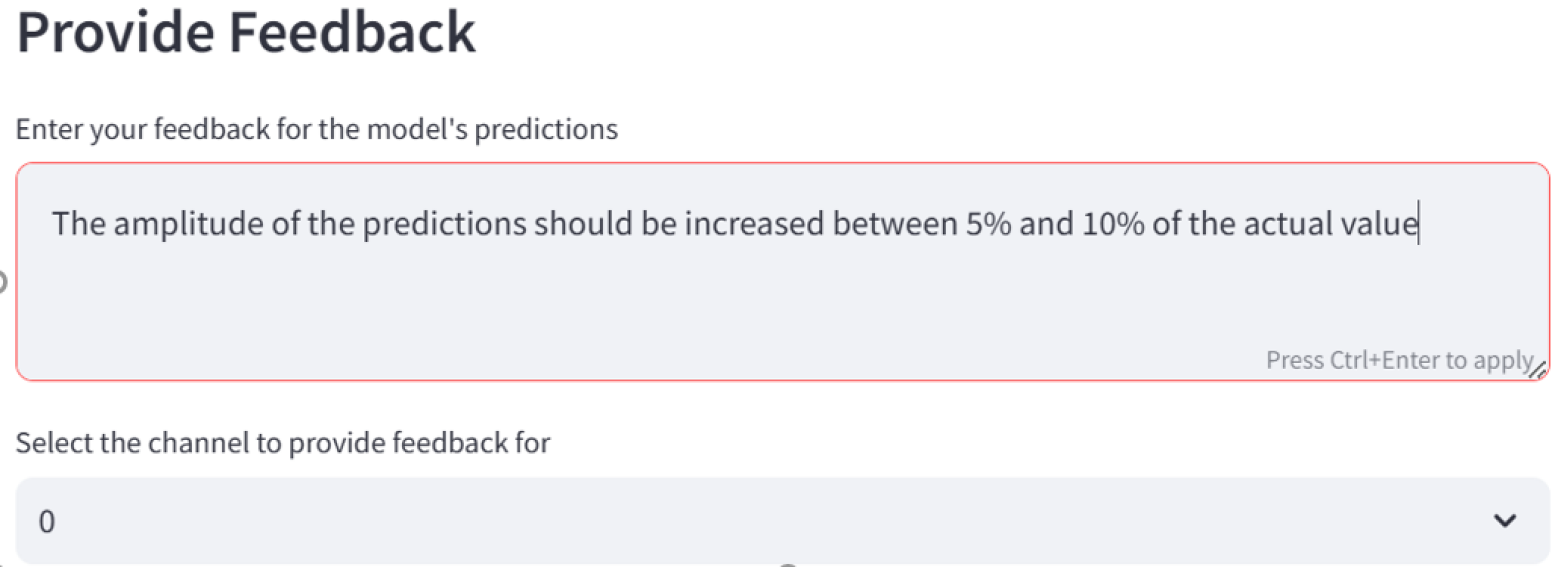
(a) User input prompt

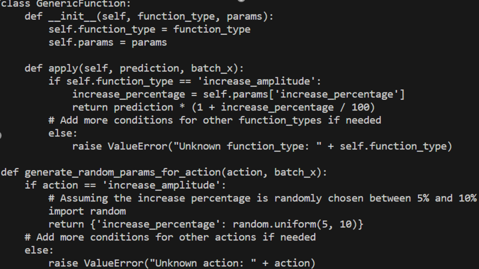
(b) Generated code for adaptive optimization

Figure 5: Transformation pipeline: From user prompt to executable code.

Interactive Refinement.

Users can iteratively refine their feedback if initial transformations are ineffective. This loop enables interpretable and low-effort adjustment without retraining, especially valuable in high-stakes or fast-changing environments.

Integration with Optimization.

The generated actions are seamlessly incorporated into the existing adaptive optimization loop (Section 3.3). The optimizer treats these transformations as part of the candidate action space, evaluating and selecting them based on validation performance.

Case Studies.

Appendix 6.4.1 presents real-world use cases where HITL feedback led to some improvements. These results demonstrate the practical value of combining human intuition with automated correction.

4 Experiments

We evaluate our framework across diverse real-world time series tasks, demonstrating consistent improvements in forecast accuracy. All experiments use standard benchmarks and open-source implementations. All experiments were conducted on a server equipped with 2× Intel Xeon E5-2690 v4 CPUs (56 cores total), 512 GB RAM, and 6× NVIDIA Tesla P100 GPUs (16 GB each), though only one GPU was used per run.

4.1 Setup

We test on datasets from energy consumption (Zhou et al.,, 2021), and several datasets from the OpenTS benchmark (Qiu et al.,, 2024). Full dataset details are in Appendix 6.2.1.

Forecasting Models. We augment forecasts from:

• Classical: DLinear (Zeng et al.,, 2023)

• Deep Learning: SegRNN (Lin et al.,, 2023), iTransformer (Liu et al.,, 2023), PatchTST (Nie et al.,, 2023), Autoformer (Wu et al.,, 2021), Crossformer (Zhang and Yan,, 2023), Informer (Zhou et al.,, 2021)

Metric. Mean Squared Error (MSE) is reported as the primary metric, averaged across multiple forecast horizons (Horizons $96$, $192$, $336$ and $792$).

4.2 Results: Adaptive Optimization Improves Forecasting

Table 2 summarizes the impact of our post-training optimization. Across nearly all models and datasets, we observe significant MSE reductions with no retraining and minimal overhead.

gray!20 Methods	Autoformer	Crossformer	iTransformer	PatchTST	DLinear	SegRNN	Informer
ETTh1	blue!10 $0.61_{\pm 0.01}\rightarrow\mathbf{0.51_{\pm 0.02}}$	blue!10 $0.54_{\pm 0.01}\rightarrow\mathbf{0.52_{\pm 0.01}}$	blue!10 $0.45_{\pm 0.01}\rightarrow\mathbf{0.44_{\pm 0.01}}$	blue!10 $0.46_{\pm 0.01}\rightarrow\mathbf{0.47_{\pm 0.01}}$	blue!10 $0.47_{\pm 0.01}\rightarrow\mathbf{0.45_{\pm 0.01}}$	blue!10 $0.47_{\pm 0.01}\rightarrow\mathbf{0.45_{\pm 0.01}}$	blue!10 $0.67_{\pm 0.01}\rightarrow\mathbf{0.65_{\pm 0.01}}$
	(16.76%)	(2.20%)	(2.58%)	(-2.25%)	(1.38%)	(1.31%)	(3.00%)
ETTh2	blue!10 $0.65_{\pm 0.01}\rightarrow\mathbf{0.55_{\pm 0.01}}$	blue!10 $0.60_{\pm 0.01}\rightarrow\mathbf{0.57_{\pm 0.01}}$	blue!10 $0.60_{\pm 0.01}\rightarrow\mathbf{0.57_{\pm 0.01}}$	blue!10 $0.60_{\pm 0.01}\rightarrow\mathbf{0.57_{\pm 0.01}}$	blue!10 $0.60_{\pm 0.01}\rightarrow\mathbf{0.57_{\pm 0.01}}$	blue!10 $0.60_{\pm 0.01}\rightarrow\mathbf{0.57_{\pm 0.01}}$	blue!10 $0.60_{\pm 0.01}\rightarrow\mathbf{0.57_{\pm 0.01}}$
	(15.48%)	(3.7%)	(4.0%)	(4.2%)	(3.8%)	(3.8%)	(3.9%)
ETTm1	blue!10 $0.60_{\pm 0.01}\rightarrow\mathbf{0.57_{\pm 0.01}}$	blue!10 $0.60_{\pm 0.01}\rightarrow\mathbf{0.57_{\pm 0.01}}$	blue!10 $0.60_{\pm 0.01}\rightarrow\mathbf{0.57_{\pm 0.01}}$	blue!10 $0.60_{\pm 0.01}\rightarrow\mathbf{0.57_{\pm 0.01}}$	blue!10 $0.60_{\pm 0.01}\rightarrow\mathbf{0.57_{\pm 0.01}}$	blue!10 $0.60_{\pm 0.01}\rightarrow\mathbf{0.57_{\pm 0.01}}$	blue!10 $0.60_{\pm 0.01}\rightarrow\mathbf{0.57_{\pm 0.01}}$
	(7.37%)	(3.7%)	(4.0%)	(4.2%)	(3.8%)	(3.8%)	(3.9%)
ETTm2	blue!10 $0.60_{\pm 0.01}\rightarrow\mathbf{0.57_{\pm 0.01}}$	blue!10 $3.82_{\pm 0.01}\rightarrow\mathbf{3.81_{\pm 0.01}}$	blue!10 $0.60_{\pm 0.01}\rightarrow\mathbf{0.57_{\pm 0.01}}$	blue!10 $0.60_{\pm 0.01}\rightarrow\mathbf{0.57_{\pm 0.01}}$	blue!10 $0.60_{\pm 0.01}\rightarrow\mathbf{0.57_{\pm 0.01}}$	blue!10 $0.60_{\pm 0.01}\rightarrow\mathbf{0.57_{\pm 0.01}}$	blue!10 $0.60_{\pm 0.01}\rightarrow\mathbf{0.57_{\pm 0.01}}$
	(20.25%)	(3.7%)	(4.0%)	(4.2%)	(3.8%)	(3.8%)	(3.9%)
Dominick	blue!10 $1.38_{\pm 0.01}\rightarrow\mathbf{1.16_{\pm 0.01}}$	blue!10 $1.12_{\pm 0.01}\rightarrow\mathbf{1.10_{\pm 0.01}}$	blue!10 $1.25_{\pm 0.01}\rightarrow\mathbf{1.23_{\pm 0.01}}$	blue!10 $1.25_{\pm 0.01}\rightarrow\mathbf{1.20_{\pm 0.01}}$	blue!10 $1.24_{\pm 0.01}\rightarrow\mathbf{1.13_{\pm 0.01}}$	blue!10 $1.92_{\pm 0.01}\rightarrow\mathbf{1.40_{\pm 0.01}}$	blue!10 $1.14_{\pm 0.01}\rightarrow\mathbf{1.09_{\pm 0.01}}$
	(15.42%)	(1.00%)	(0.89%)	(3.83%)	(7.97%)	(27.21%)	(4.28%)
Human	blue!10 $0.40_{\pm 0.01}\rightarrow\mathbf{0.33_{\pm 0.01}}$	blue!10 $0.30_{\pm 0.01}\rightarrow\mathbf{0.25_{\pm 0.01}}$	blue!10 $0.60_{\pm 0.01}\rightarrow\mathbf{0.15_{\pm 0.01}}$	blue!10 $0.62_{\pm 0.01}\rightarrow\mathbf{0.15_{\pm 0.01}}$	blue!10 $0.96_{\pm 0.01}\rightarrow\mathbf{0.26_{\pm 0.01}}$	blue!10 $0.60_{\pm 0.01}\rightarrow\mathbf{0.25_{\pm 0.01}}$	blue!10 $0.30_{\pm 0.01}\rightarrow\mathbf{0.21_{\pm 0.01}}$
	(20.24%)	(13.34%)	(51.26%)	(51.74%)	(57.85%)	(43.02%)	(21.93%)
KDD	blue!10 $1.25_{\pm 0.01}\rightarrow\mathbf{0.95_{\pm 0.01}}$	blue!10 $0.80_{\pm 0.01}\rightarrow\mathbf{0.80_{\pm 0.01}}$	blue!10 $1.13_{\pm 0.01}\rightarrow\mathbf{0.88_{\pm 0.01}}$	blue!10 $1.14_{\pm 0.01}\rightarrow\mathbf{0.89_{\pm 0.01}}$	blue!10 $0.93_{\pm 0.01}\rightarrow\mathbf{0.85_{\pm 0.01}}$	blue!10 $1.10_{\pm 0.01}\rightarrow\mathbf{0.88_{\pm 0.01}}$	blue!10 $1.12_{\pm 0.01}\rightarrow\mathbf{0.87_{\pm 0.01}}$
	(23.50%)	(-0.03%)	(21.09%)	(21.83%)	(8.54%)	(19.14%)	(22.15%)
Nature	blue!10 $1.25_{\pm 0.01}\rightarrow\mathbf{0.96_{\pm 0.01}}$	blue!10 $0.65_{\pm 0.01}\rightarrow\mathbf{0.66_{\pm 0.01}}$	blue!10 $0.34_{\pm 0.01}\rightarrow\mathbf{0.33_{\pm 0.01}}$	blue!10 $0.26_{\pm 0.01}\rightarrow\mathbf{0.25_{\pm 0.01}}$	blue!10 $0.95_{\pm 0.01}\rightarrow\mathbf{0.91_{\pm 0.01}}$	blue!10 $1.02_{\pm 0.01}\rightarrow\mathbf{0.94_{\pm 0.01}}$	blue!10 $0.91_{\pm 0.01}\rightarrow\mathbf{0.90_{\pm 0.01}}$
	(21.69%)	(-1.17%)	(3.26%)	(3.72%)	(4.31%)	(8.67%)	(0.86%)
NASDAQ	blue!10 $0.91_{\pm 0.01}\rightarrow\mathbf{0.70_{\pm 0.01}}$	blue!10 $0.46_{\pm 0.01}\rightarrow\mathbf{0.46_{\pm 0.01}}$	blue!10 $0.80_{\pm 0.01}\rightarrow\mathbf{0.63_{\pm 0.01}}$	blue!10 $0.79_{\pm 0.01}\rightarrow\mathbf{0.68_{\pm 0.01}}$	blue!10 $0.74_{\pm 0.01}\rightarrow\mathbf{0.68_{\pm 0.01}}$	blue!10 $0.78_{\pm 0.01}\rightarrow\mathbf{0.62_{\pm 0.01}}$	blue!10 $0.85_{\pm 0.01}\rightarrow\mathbf{0.79_{\pm 0.01}}$
	(22.39%)	(-0.33%)	(19.77%)	(14.76%)	(7.59%)	(19.19%)	(8.96%)
Pedestrian	blue!10 $0.46_{\pm 0.01}\rightarrow\mathbf{0.27_{\pm 0.01}}$	blue!10 $0.14_{\pm 0.01}\rightarrow\mathbf{0.13_{\pm 0.01}}$	blue!10 $0.14_{\pm 0.01}\rightarrow\mathbf{0.12_{\pm 0.01}}$	blue!10 $0.22_{\pm 0.01}\rightarrow\mathbf{0.19_{\pm 0.01}}$	blue!10 $0.69_{\pm 0.01}\rightarrow\mathbf{0.60_{\pm 0.01}}$	blue!10 $0.20_{\pm 0.01}\rightarrow\mathbf{0.18_{\pm 0.01}}$	blue!10 $0.33_{\pm 0.01}\rightarrow\mathbf{0.27_{\pm 0.01}}$
	(40.01%)	(0.26%)	(9.43%)	(9.54%)	(14.20%)	(6.94%)	(15.87%)
Tourism	blue!10 $0.24_{\pm 0.01}\rightarrow\mathbf{0.22_{\pm 0.01}}$	blue!10 $0.16_{\pm 0.01}\rightarrow\mathbf{0.14_{\pm 0.01}}$	blue!10 $0.31_{\pm 0.01}\rightarrow\mathbf{0.14_{\pm 0.01}}$	blue!10 $0.31_{\pm 0.01}\rightarrow\mathbf{0.14_{\pm 0.01}}$	blue!10 $0.52_{\pm 0.01}\rightarrow\mathbf{0.25_{\pm 0.01}}$	blue!10 $0.24_{\pm 0.01}\rightarrow\mathbf{0.12_{\pm 0.01}}$	blue!10 $0.22_{\pm 0.01}\rightarrow\mathbf{0.18_{\pm 0.01}}$
	(10.88%)	(11.48%)	(40.08%)	(39.20%)	(48.91%)	(48.14%)	(20.57%)
Vehicle trips	blue!10 $1.39_{\pm 0.01}\rightarrow\mathbf{1.13_{\pm 0.01}}$	blue!10 $0.83_{\pm 0.01}\rightarrow\mathbf{0.82_{\pm 0.01}}$	blue!10 $1.02_{\pm 0.01}\rightarrow\mathbf{0.84_{\pm 0.01}}$	blue!10 $0.98_{\pm 0.01}\rightarrow\mathbf{0.80_{\pm 0.01}}$	blue!10 $1.35_{\pm 0.01}\rightarrow\mathbf{1.15_{\pm 0.01}}$	blue!10 $1.68_{\pm 0.01}\rightarrow\mathbf{1.05_{\pm 0.01}}$	blue!10 $1.21_{\pm 0.01}\rightarrow\mathbf{0.95_{\pm 0.01}}$
	(18.13%)	(0.89%)	(17.14%)	(18.00%)	(14.37%)	(38.46%)	(21.54%)

Table 2: Mean squared error (MSE) ± standard deviation across multiple forecast horizons, before and after applying Adaptive Optimization ($\rightarrow$). Improvements are reported in teal when positive and orange when negative.

4.2.1 Human-in-the-Loop Feedback

Human feedback can further enhance forecast accuracy by introducing domain knowledge not captured by the base model. Users provide natural language instructions (e.g., "increase the amplitude of predictions below 0.5"), which are converted into executable transformations via a large language model (LLM).

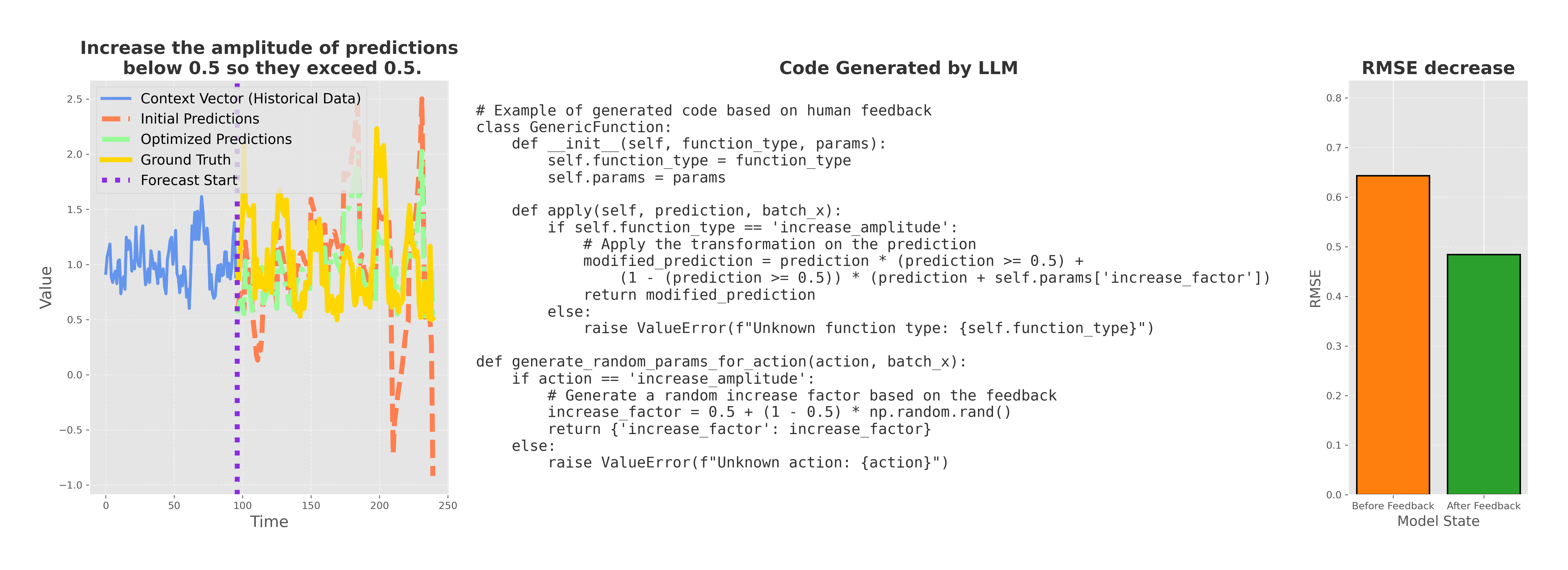
Figure 6: (a) Initial prediction vs. human-refined forecast. (b) Action code generated from natural language via LLM (qwen2-72b-32k). (c) RMSE improvement post-feedback.

Figure 6 shows that integrating expert suggestions via HITL leads to tangible performance gains. Additional examples are presented in Appendix 6.4. The interface supports real-time experimentation, making human-guided optimization practical and intuitive.

4.2.2 Computational Efficiency and Scalability

We evaluate optimization time across varying forecast horizons and action space sizes on the ETTh1 dataset. Table 3 compares our post-training augmentation time against the minimum and maximum training times of standard forecasting models.

Table 3: Adaptive optimization time vs. base model training time (10 epochs).

Horizon	2 Actions	4 Actions	7 Actions	DLinear (min)	PatchTST (max)
96	3.2s ± 0.1	5.4s ± 0.2	12.0s ± 1.3	gray!2020.3s	gray!20144.4s
192	6.1s ± 0.3	9.7s ± 0.4	22.7s ± 1.5	gray!2022.3s	gray!20146.2s
336	12.7s ± 0.5	18.3s ± 0.6	30.1s ± 1.0	gray!2024.4s	gray!20148.8s
720	24.3s ± 1.1	35.2s ± 1.4	45.1s ± 1.8	gray!2027.3s	gray!20151.8s

Even for long horizons and expanded action spaces, our optimization time remains well below the training cost of most models. This confirms the framework’s suitability for real-time applications and large-scale deployment.

5 Conclusion

We introduced a model-agnostic framework for time series forecasting that improves accuracy through post-training adaptive optimization and optional human-in-the-loop refinement. Unlike traditional approaches that require retraining or architecture changes, our method applies lightweight, interpretable transformations to enhance predictions.

Experiments across diverse datasets and models show consistent improvements with minimal computational cost. Additionally, human feedback—expressed in natural language—can be seamlessly integrated via an LLM-to-action pipeline.

Key strengths of our framework include:

• Compatibility with any forecasting model—no retraining required.

• Fast and interpretable post-hoc corrections via optimization.

• Optional human-in-the-loop refinement using natural language.

Future work will explore more expressive transformations, tighter LLM-feedback alignment, and integration with multimodal and streaming time series systems.

Limitations.

While our framework is broadly applicable and efficient, several limitations remain. First, the effectiveness of post-training corrections depends on the quality of the base model’s initial predictions; if the model is highly inaccurate or erratic, corrective transformations may offer limited benefit. Second, although we support natural language feedback via large language models (LLMs), the precision of action translation can vary with instruction clarity and model alignment. Robustness under ambiguous or contradictory feedback remains an open challenge. Finally, our current implementation assumes access to a validation set that reflects the deployment distribution—performance may degrade under distribution shift.

6 Supplementary Material

Human-in-the-Loop Adaptive Optimization for Improved Time Series Forecasting

Table of Contents

1. 1 Introduction
2. 2 Related Work
3. 3 Methodology
   1. 3.1 Theoretical Motivation for Post-Training Correction
   2. 3.2 Forecasting Model Setup
   3. 3.3 Post-Training Optimization via Action Space
      1. 3.3.1 Optimizing Actions and Parameters
      2. 3.3.2 Dynamic Optimization Strategies
      3. 3.3.3 Why Discrete Actions + Continuous Parameters Work
   4. 3.4 Optimization Strategy: Empirical Comparison
   5. 3.5 Human-in-the-Loop Feedback Integration
4. 4 Experiments
   1. 4.1 Setup
   2. 4.2 Results: Adaptive Optimization Improves Forecasting
      1. 4.2.1 Human-in-the-Loop Feedback
      2. 4.2.2 Computational Efficiency and Scalability
5. 5 Conclusion
6. 6 Supplementary Material
7. 6.1 Mathematical definitions and visualizations of the pool of actions
8. 6.2 Details on experimental setup: Datasets and models
   1. 6.2.1 Datasets
   2. 6.2.2 Time Series Models
9. 6.3 More experiments on the reinforcement automated loop
   1. 6.3.1 Comparison between optimization strategy over the pool of actions
   2. 6.3.2 Experiments for the SH-HPO on all datasets and horizons
10. 6.4 More experiments on the human feedback
    1. 6.4.1 Human Feedback in Action
11. 6.5 Code and Reproducibility
12. 6.6 Code Usage and API Documentation
13. 6.6.1 Examples to Use the Streamlit Application
14. 6.7 Installation and usage for development
15. 6.8 Theoretical motivation for post training in time series forecasting
    1. 6.8.1 Problem Setup
    2. 6.8.2 Derivation of Optimal Correction Parameters
    3. 6.8.3 Theoretical Risk Before and After Correction
    4. 6.8.4 Comparison of Risks
    5. 6.8.5 Conclusion

Abstract

This supplementary material provides an extended discussion and additional details supporting the main paper on Human-in-the-Loop Adaptive Optimization for Improved Time Series Forecasting. We first delve deeper into the mathematical formulation of the different actions used in our framework, offering visualizations to better illustrate their roles and impacts on model performance.

Next, we provide an in-depth exploration of the adaptive optimization algorithms employed within our approach, detailing their integration into state-of-the-art time series forecasting models. Supplementary experiments are included to showcase the effectiveness of our adaptive optimization -enhanced models across various datasets, comparing them against baseline methods to highlight performance improvements.

Human feedback is also a central aspect of our framework. In this section, we demonstrate how human feedback can be integrated into the post-training process through several real-world examples, illustrating the subjective nature of human input and its positive impact on model fine-tuning.

Finally, we offer detailed instructions on how to reproduce the experiments and results presented in this work. This includes guidance on using the provided code and graphical interface, enabling users to easily test and customize our framework for their own time series forecasting tasks. All code and resources are made publicly available for further exploration and use by the research community.

6.1 Mathematical definitions and visualizations of the pool of actions

Before presenting the mathematical definitions in the table, let’s define the notation used in the transformations:

• $\mathbf{x}$: The original time series or predictions (before transformation), where each $x_{t}$ is the value at time $t$.

• $\mathbf{y}$: The transformed time series or predictions, resulting from applying one of the post-training actions.

• $x_{t}$: The value at time step $t$ in the original time series.

• $y_{t}$: The transformed value at time step $t$ in the new series.

• $x_{\max}$: The maximum value in the time series $\mathbf{x}$ across all time steps.

• $x_{\min}$: The minimum value in the time series $\mathbf{x}$ across all time steps.

• $\bar{x}$: The average value of the time series $\mathbf{x}$ over all time steps.

• $Q_{\delta}$: The $\delta$-th quantile of the values in $\mathbf{x}$, which corresponds to the value at the specified percentile of the distribution of $\mathbf{x}$.

• $\Delta$: The amount by which to shift the time series in the "Shift Series" action (in terms of time steps).

• $s$: The slope parameter for adding a linear trend to the time series, representing a change in the amplitude of the series over time.

• $b$: The intercept parameter for adding a linear trend to the time series, adjusting the average level of the series.

• $f$: The factor used in scaling operations, such as scaling the amplitude or adjusting the minimum/maximum values.

• $\sigma$: The standard deviation parameter for noise addition, influencing the spread of the generated noise.

• $t$: The time step index, which ranges from 1 to $H$, where $H$ is the total number of time steps (the horizon) in the time series.

The following table summarizes each action’s mathematical operation and the continuous parameters involved, along with their respective ranges.

Action Name	Mathematical Definition	Continuous Parameters (Range)
gray!10 Trend Modifications
Linear Trend Slope	$\mathbf{y}=\mathbf{x}+\left(\frac{s}{100}\cdot(x_{\max}-x_{\min})\right)\cdot t$	$s\in(-5,5)$, $t\in[H]$
Linear Trend Intercept	$\mathbf{y}=\mathbf{x}+\left(\frac{b}{100}\cdot\bar{x}\right)$	$b\in(-5,5)$
gray!10 Piecewise Scaling
Piecewise Scale High	$\mathbf{y}=\mathbf{x}\cdot\left(1+\frac{f}{100}\right)\ \text{for}\ x_{t}\leq Q_{\delta}$	$\delta\in(70,100)$, $f\in(-1,10)$
Piecewise Scale Low	$\mathbf{y}=\mathbf{x}\cdot\left(1+\frac{f}{100}\right)\ \text{for}\ x_{t}>Q_{\delta}$	$\delta\in(0,30)$, $f\in(-1,10)$
gray!10 Frequency and Phase
Swap Series	$y_{t}=-\left(\mathbf{x}-\bar{x}\right)+\bar{x}$	None
Shift Series	$y_{t}=x_{t+\Delta}$	$\Delta\in(-200,200)$
gray!10 Amplitude Modifications
Scale Amplitude	$\mathbf{y}=\mathbf{x}\cdot\left(1+\frac{f}{100}\right)$	$f\in(-5,5)$
Add Noise	$\mathbf{y}=\mathbf{x}+\epsilon\ \text{where}\ \epsilon\sim\mathcal{N}(0,\frac{\sigma}{100}\cdot|x_{t}|)$	$\sigma\in(10,30)$
Increase Minimum Factor	$\mathbf{y}=\mathbf{x}\cdot(1+\frac{f}{100})\ \text{for}\ x_{t}\leq Q_{10\%}$	$f\in(-1,10)$

Table 4: Mathematical definitions and continuous parameters for each post-training action. The range for each parameter is specified to guide the tuning of each transformation. Note: $x_{t}$ is the initial prediction and $y_{t}$ is the transformed prediction for each sample and each dimension. $x_{\max}$ and $x_{\min}$ are minimum and maximum values of $x_{t}$ over all horizons $H$ and $\bar{x}$ is the average value. $Q_{\delta}$ is the $\delta$-quantile of the vector $\mathbf{x}$.

These post-training actions modify time series predictions through mathematical transformations targeting trends, amplitudes, and frequency/phase. Each transformation is defined mathematically, with adjustable parameters like scaling factors and thresholds to optimize performance.

Figure 7 shows the original time series alongside the transformed series, with each subplot illustrating a different post-training action applied.

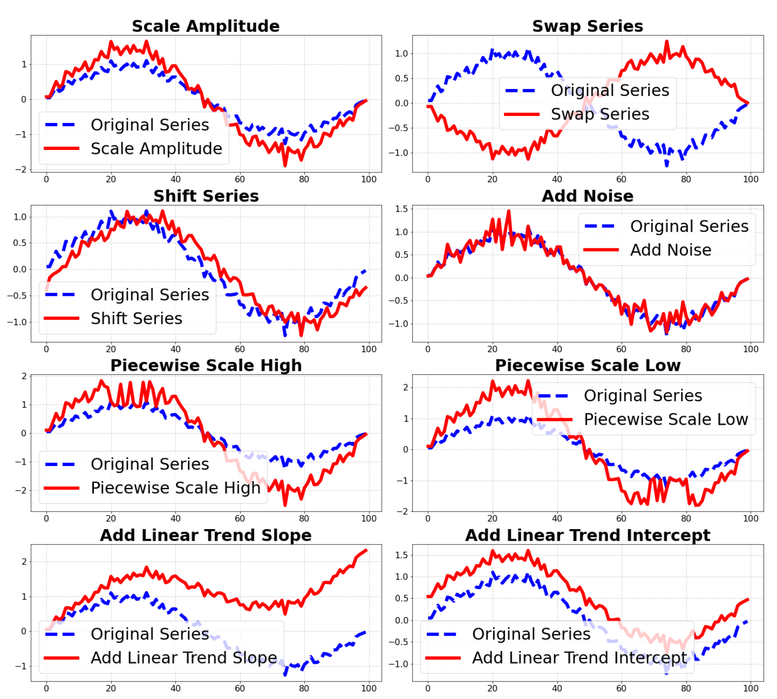
Figure 7: Visual representation of the time series transformations. Each subplot illustrates a different post-training action applied to the original time series.

6.2 Details on experimental setup: Datasets and models

6.2.1 Datasets

In this section, we provide a summary of the datasets used in our analysis. The following table outlines the dataset names, their sources, key characteristics, and the corresponding references for the papers that describe each dataset.

Table 5: Datasets Overview

gray!20 Dataset Name	Source and Reference	Characteristics
ETTh1	ETTh (Electricity) Benchmark Zhou et al., (2021)	1-hour-level time-series with 6 features and "oil temperature" as the target. Train/val/test split: 12/4/4 months.
ETTh2	ETTh (Electricity) Benchmark Zhou et al., (2021)	1-hour-level time-series with 6 features and "oil temperature" as the target. Includes more features than ETTh1.
ETTm1	ETTh (Electricity) Benchmark Zhou et al., (2021)	15-minute-level time-series with 6 features and "oil temperature" as the target. Train/val/test split: 12/4/4 months.
ETTm2	ETTh (Electricity) Benchmark Zhou et al., (2021)	15-minute-level time-series, similar to ETTm1, with different subsets for long-term forecasting.
Dominick	Open TS Benchmark Qiu et al., (2024)	115704 weekly time series representing the profit of individual stock keeping units from a retailer.
Nature	Open TS Benchmark Qiu et al., (2024)
Human	Open TS Benchmark Qiu et al., (2024)	Time-series data for human activity recognition, captured by wearable devices.
NASDAQ	Open TS Benchmark Qiu et al., (2024)	Stock market data from NASDAQ. Used for financial forecasting challenges.
KDD Cup	Open TS Benchmark Qiu et al., (2024)
Pedestrian	Open TS Benchmark Qiu et al., (2024)	Pedestrian count data from urban settings, used for mobility prediction.
Tourism	Open TS Benchmark Qiu et al., (2024)	Tourism demand data, used for forecasting seasonal trends.
Vehicle Trips	Open TS Benchmark Qiu et al., (2024)	Vehicle trip data, used for urban mobility and traffic pattern forecasting.

6.2.2 Time Series Models

In this work, we utilize several state-of-the-art time series forecasting models, all of which are part of the framework described in Liu et al., 2024b . These models are trained for 10 epochs, with early stopping applied on the validation set to prevent overfitting. Below, we briefly describe each of the models used:

• Autoformer Wu et al., (2021): A deep learning model designed to capture long-term dependencies and seasonality in time-series data by leveraging an attention mechanism.

• Crossformer Zhang and Yan, (2023): This model integrates cross-attention mechanisms to effectively model both long-range and local dependencies in time-series forecasting.

• PatchTST Nie et al., (2023): A vision transformer-based model that divides time-series data into patches to capture temporal dependencies, providing superior performance in forecasting.

• DLinear Zeng et al., (2023): A linear decomposition model that separates the time series into trend and seasonal components for more interpretable and efficient forecasting.

• Informer Zhou et al., (2021): A transformer-based model that focuses on efficiency for long-term forecasting by using a self-attention mechanism and probabilistic forecast outputs.

• SegRNN Lin et al., (2023): A sequential deep learning model that combines segmentation with recurrent neural networks to handle irregular time-series data.

Each of these models has demonstrated strong performance in time series forecasting tasks, and we have used them to compare their abilities on the datasets described earlier.

6.3 More experiments on the reinforcement automated loop

6.3.1 Comparison between optimization strategy over the pool of actions

We compare the performance of four different classes of algorithms:

1. Random search where each discrete action is evaluated by randomly sampling continuous parameters and selecting the best-performing configuration.

2. Bandit algorithm, which considers each class of actions as an arm and optimizes using line search the parameter called SH-HPO.

3. Reinforcement learning algorithm (PPO), which discretizes the set of actions and implements the PPO algorithm (Schulman et al.,, 2017) denoted RL(PPO).

4. Genetic algorithm (GA) (Sampson,, 1976), which discretizes the set of actions and performs a genetic algorithm denoted GA.

We present the result for several time series models and for five different datasets in Table 6.

The metric used to measure the efficiency of post-training is the relative decrease in Mean Squared Error (MSE) observed after post-training. Specifically, given the MSE before post-training, $\textit{MSE}_{\text{before}}$, and the MSE after post-training, $\textit{MSE}_{\text{after}}$, the relative decrease in MSE, $\mathcal{M}$, is calculated as:

$$\mathcal{M}=\frac{\textit{MSE}_{\text{before}}-\textit{MSE}_{\text{after}}}{\textit{MSE}_{\text{before}}}$$ (2)

A positive value of $\mathcal{M}$ indicates that post-training has reduced the MSE, with larger positive values signifying greater improvement. Conversely, a negative value indicates degradation compared to the initial prediction.

gray!20 Models	Datasets	Random	SH-HPO	RL (PPO)	GA
Autoformer	ETTh1 (96)	12.77%	19.85%	2.71%	6.76%
	ETTh1 (192)	18.42%	17.32%	3.14%	6.20%
	ETTh1 (336)	13.09%	12.91%	3.54%	4.43%
	ETTh1 (792)	24.48%	27.26%	4.02%	6.96%
	Average	17.19%	19.34%	3.35%	6.09%
Crossformer	ETTh1 (96)	5.49%	4.01%	2.71%	0.16%
	ETTh1 (192)	2.05%	3.80%	1.71%	3.48%
	ETTh1 (336)	3.13%	3.13%	0.14%	1.37%
	ETTh1 (792)	2.53%	0.17%	-0.14%	1.07%
	Average	3.30%	2.78%	1.11%	1.52%
PatchTST	ETTh1 (96)	-0.99%	0.15%	0.40%	0.62%
	ETTh1 (192)	-0.06%	-1.13%	0.12%	0.23%
	ETTh1 (336)	-3.13%	0.23%	0.41%	0.19%
	ETTh1 (772)	-1.12%	-2.50%	0.12%	0.14%
	Average	-1.33%	-0.81%	0.26%	0.29%
SegRNN	ETTh1 (96)	0.80%	1.22%	0.13%	0.06%
	ETTh1 (192)	1.24%	1.56%	0.73%	0.68%
	ETTh1 (336)	2.38%	3.76%	0.71%	0.36%
	ETTh1 (772)	2.39%	3.81%	0.87%	1.26%
	Average	1.70%	2.59%	0.61%	0.59%
DLinear	ETTh1 (96)	1.50%	1.40%	0.97%	1.24%
	ETTh1 (192)	2.03%	2.18%	1.39%	2.35%
	ETTh1 (336)	2.96%	5.07%	4.62%	3.96%
	ETTh1 (772)	1.33%	-2.37%	1.82%	-1.11%
	Average	1.96%	1.57%	2.20%	1.61%
Informer	ETTh1 (96)	12.98%	6.83%	6.12%	4.87%
	ETTh1 (192)	8.89%	7.28%	3.74%	2.17%
	ETTh1 (336)	1.68%	4.01%	3.81%	2.49%
	ETTh1 (772)	-3.80%	3.61%	0.26%	0.94%
	Average	4.94%	5.43%	3.48%	2.62%
iTransformer	ETTh1 (96)	2.16%	4.83%	0.41%	1.05%
	ETTh1 (192)	2.79%	1.89%	1.26%	1.03%
	ETTh1 (336)	3.22%	4.01%	1.32%	1.78%
	ETTh1 (772)	4.23%	4.67%	2.34%	2.15%
	Average	3.10%	3.85%	1.33%	1.50%
Overall Average		4.83%	5.65%	1.62%	2.12%

Table 6: Results of applying different algorithms (Random, SH-HPO, RL (PPO), GA) to various time series forecasting models and datasets. Each cell shows the observed improvement for the respective algorithm, model, and dataset. The improvements are measured in percentage points.

Figure 8: Average improvement across all models and datasets for each method.

6.3.2 Experiments for the SH-HPO on all datasets and horizons

gray!20 Methods		Autoformer	Crossformer	iTransformer	PatchTST	DLinear	SegRNN	Informer
ETTh1		blue!10 $0.52_{\pm 0.04}\rightarrow\mathbf{0.45_{\pm 0.03}}$	blue!10 $0.41_{\pm 0.02}\rightarrow\mathbf{0.39_{\pm 0.01}}$	blue!10 $0.41_{\pm 0.02}\rightarrow\mathbf{0.40_{\pm 0.01}}$	blue!10 $0.40_{\pm 0.02}\rightarrow 0.41_{\pm 0.01}$	blue!10 $0.41_{\pm 0.02}\rightarrow\mathbf{0.40_{\pm 0.01}}$	blue!10 $0.39_{\pm 0.02}\rightarrow\mathbf{0.38_{\pm 0.01}}$	blue!10 $0.57_{\pm 0.02}\rightarrow\mathbf{0.56_{\pm 0.01}}$
		(12.94%)	(3.41%)	(1.97%)	(-1.31%)	(1.47%)	(1.22%)	(1.55%)
		blue!10 $0.59_{\pm 0.03}\rightarrow\mathbf{0.48_{\pm 0.02}}$	blue!10 $0.48_{\pm 0.02}\rightarrow\mathbf{0.46_{\pm 0.02}}$	blue!10 $0.45_{\pm 0.03}\rightarrow\mathbf{0.44_{\pm 0.02}}$	blue!10 $0.44_{\pm 0.03}\rightarrow\mathbf{0.44_{\pm 0.02}}$	blue!10 $0.46_{\pm 0.03}\rightarrow\mathbf{0.45_{\pm 0.02}}$	blue!10 $0.43_{\pm 0.03}\rightarrow\mathbf{0.42_{\pm 0.02}}$	blue!10 $0.67_{\pm 0.03}\rightarrow\mathbf{0.62_{\pm 0.02}}$
		(17.75%)	(3.43%)	(2.77%)	(-0.94%)	(2.15%)	(1.58%)	(7.10%)
		blue!10 $0.65_{\pm 0.02}\rightarrow\mathbf{0.57_{\pm 0.01}}$	blue!10 $0.59_{\pm 0.02}\rightarrow\mathbf{0.58_{\pm 0.01}}$	blue!10 $0.49_{\pm 0.02}\rightarrow\mathbf{0.47_{\pm 0.01}}$	blue!10 $0.47_{\pm 0.02}\rightarrow\mathbf{0.48_{\pm 0.01}}$	blue!10 $0.50_{\pm 0.02}\rightarrow\mathbf{0.48_{\pm 0.01}}$	blue!10 $0.50_{\pm 0.02}\rightarrow\mathbf{0.47_{\pm 0.01}}$	blue!10 $0.70_{\pm 0.02}\rightarrow\mathbf{0.68_{\pm 0.01}}$
		(11.51%)	(0.67%)	(3.54%)	(-3.38%)	(2.58%)	(1.31%)	(2.56%)
		blue!10 $0.71_{\pm 0.02}\rightarrow\mathbf{0.53_{\pm 0.03}}$	blue!10 $0.70_{\pm 0.02}\rightarrow\mathbf{0.68_{\pm 0.01}}$	blue!10 $0.48_{\pm 0.02}\rightarrow\mathbf{0.47_{\pm 0.01}}$	blue!10 $0.55_{\pm 0.02}\rightarrow\mathbf{0.56_{\pm 0.01}}$	blue!10 $0.51_{\pm 0.02}\rightarrow\mathbf{0.50_{\pm 0.01}}$	blue!10 $0.55_{\pm 0.02}\rightarrow\mathbf{0.52_{\pm 0.01}}$	blue!10 $0.75_{\pm 0.02}\rightarrow\mathbf{0.74_{\pm 0.01}}$
		(24.85%)	(2.76%)	(2.05%)	(-3.37%)	(-0.68%)	(1.04%)	(0.75%)
		blue!10 $0.61_{\pm 0.01}\rightarrow\mathbf{0.51_{\pm 0.02}}$	blue!10 $0.54_{\pm 0.01}\rightarrow\mathbf{0.52_{\pm 0.01}}$	blue!10 $0.45_{\pm 0.01}\rightarrow\mathbf{0.44_{\pm 0.01}}$	blue!10 $0.46_{\pm 0.01}\rightarrow\mathbf{0.47_{\pm 0.01}}$	blue!10 $0.47_{\pm 0.01}\rightarrow\mathbf{0.45_{\pm 0.01}}$	blue!10 $0.47_{\pm 0.01}\rightarrow\mathbf{0.45_{\pm 0.01}}$	blue!10 $0.67_{\pm 0.01}\rightarrow\mathbf{0.65_{\pm 0.01}}$
		(16.76%)	(2.20%)	(2.58%)	(-2.25%)	(1.38%)	(1.31%)	(3.00%)
ETTh2		blue!10 $0.55_{\pm 0.02}\rightarrow\mathbf{0.44_{\pm 0.01}}$	blue!10 $1.10_{\pm 0.02}\rightarrow\mathbf{1.04_{\pm 0.01}}$	blue!10 $0.33_{\pm 0.02}\rightarrow\mathbf{0.32_{\pm 0.01}}$	blue!10 $0.32_{\pm 0.02}\rightarrow\mathbf{0.31_{\pm 0.01}}$	blue!10 $0.38_{\pm 0.02}\rightarrow\mathbf{0.33_{\pm 0.01}}$	blue!10 $0.31_{\pm 0.02}\rightarrow\mathbf{0.30_{\pm 0.01}}$	blue!10 $0.38_{\pm 0.02}\rightarrow\mathbf{0.37_{\pm 0.01}}$
		(20.87%)	(5.38%)	(2.45%)	(3.23%)	(15.12%)	(3.51%)	(1.89%)
		blue!10 $0.78_{\pm 0.03}\rightarrow\mathbf{0.64_{\pm 0.02}}$	blue!10 $1.59_{\pm 0.03}\rightarrow\mathbf{1.58_{\pm 0.02}}$	blue!10 $0.40_{\pm 0.03}\rightarrow\mathbf{0.39_{\pm 0.02}}$	blue!10 $0.40_{\pm 0.03}\rightarrow\mathbf{0.39_{\pm 0.02}}$	blue!10 $0.50_{\pm 0.03}\rightarrow\mathbf{0.47_{\pm 0.02}}$	blue!10 $0.39_{\pm 0.03}\rightarrow\mathbf{0.38_{\pm 0.02}}$	blue!10 $0.51_{\pm 0.03}\rightarrow\mathbf{0.47_{\pm 0.02}}$
		(18.65%)	(0.58%)	(1.60%)	(1.87%)	(6.54%)	(-5.88%)	(7.13%)
		blue!10 $0.75_{\pm 0.02}\rightarrow\mathbf{0.63_{\pm 0.01}}$	blue!10 $6.57_{\pm 0.02}\rightarrow\mathbf{6.57_{\pm 0.01}}$	blue!10 $0.44_{\pm 0.02}\rightarrow\mathbf{0.43_{\pm 0.01}}$	blue!10 $0.43_{\pm 0.02}\rightarrow 0.44_{\pm 0.01}$	blue!10 $0.61_{\pm 0.02}\rightarrow\mathbf{0.57_{\pm 0.01}}$	blue!10 $0.50_{\pm 0.02}\rightarrow\mathbf{0.47_{\pm 0.01}}$	blue!10 $0.46_{\pm 0.02}\rightarrow\mathbf{0.44_{\pm 0.01}}$
		(16.69%)	(0.00%)	(2.98%)	(-2.40%)	(6.15%)	(3.61%)	(3.84%)
		blue!10 $0.55_{\pm 0.02}\rightarrow\mathbf{0.52_{\pm 0.01}}$	blue!10 $0.55_{\pm 0.02}\rightarrow\mathbf{0.52_{\pm 0.01}}$	blue!10 $0.49_{\pm 0.02}\rightarrow\mathbf{0.48_{\pm 0.01}}$	blue!10 $0.43_{\pm 0.02}\rightarrow\mathbf{0.40_{\pm 0.01}}$	blue!10 $0.85_{\pm 0.02}\rightarrow\mathbf{0.79_{\pm 0.01}}$	blue!10 $0.55_{\pm 0.02}\rightarrow\mathbf{0.52_{\pm 0.01}}$	blue!10 $0.43_{\pm 0.02}\rightarrow\mathbf{0.42_{\pm 0.01}}$
		(5.69%)	(-0.01%)	(4.13%)	(5.05%)	(6.70%)	(1.31%)	(0.44%)
		blue!10 $0.65_{\pm 0.01}\rightarrow\mathbf{0.55_{\pm 0.01}}$	blue!10 $0.60_{\pm 0.01}\rightarrow\mathbf{0.57_{\pm 0.01}}$	blue!10 $0.60_{\pm 0.01}\rightarrow\mathbf{0.57_{\pm 0.01}}$	blue!10 $0.60_{\pm 0.01}\rightarrow\mathbf{0.57_{\pm 0.01}}$	blue!10 $0.60_{\pm 0.01}\rightarrow\mathbf{0.57_{\pm 0.01}}$	blue!10 $0.60_{\pm 0.01}\rightarrow\mathbf{0.57_{\pm 0.01}}$	blue!10 $0.60_{\pm 0.01}\rightarrow\mathbf{0.57_{\pm 0.01}}$
		(15.48%)	(3.7%)	(4.0%)	(4.2%)	(3.8%)	(3.8%)	(3.9%)
ETTm1		blue!10 $0.43_{\pm 0.02}\rightarrow\mathbf{0.40_{\pm 0.01}}$	blue!10 $0.39_{\pm 0.02}\rightarrow\mathbf{0.38_{\pm 0.01}}$	blue!10 $0.21_{\pm 0.02}\rightarrow\mathbf{0.20_{\pm 0.01}}$	blue!10 $0.36_{\pm 0.02}\rightarrow\mathbf{0.34_{\pm 0.01}}$	blue!10 $0.37_{\pm 0.02}\rightarrow\mathbf{0.35_{\pm 0.01}}$	blue!10 $0.35_{\pm 0.02}\rightarrow\mathbf{0.34_{\pm 0.01}}$	blue!10 $0.71_{\pm 0.02}\rightarrow\mathbf{0.64_{\pm 0.01}}$
		(3.73%)	(2.60%)	(2.52%)	(4.53%)	(5.05%)	(2.71%)	(9.98%)
		blue!10 $0.67_{\pm 0.03}\rightarrow\mathbf{0.62_{\pm 0.02}}$	blue!10 $0.53_{\pm 0.03}\rightarrow\mathbf{0.50_{\pm 0.02}}$	blue!10 $0.27_{\pm 0.03}\rightarrow\mathbf{0.25_{\pm 0.02}}$	blue!10 $0.38_{\pm 0.03}\rightarrow\mathbf{0.37_{\pm 0.02}}$	blue!10 $0.40_{\pm 0.03}\rightarrow\mathbf{0.38_{\pm 0.02}}$	blue!10 $0.38_{\pm 0.03}\rightarrow\mathbf{0.37_{\pm 0.02}}$	blue!10 $0.72_{\pm 0.03}\rightarrow\mathbf{0.70_{\pm 0.02}}$
		(6.31%)	(5.24%)	(2.42%)	(2.27%)	(3.62%)	(2.34%)	(2.92%)
		blue!10 $0.73_{\pm 0.02}\rightarrow\mathbf{0.68_{\pm 0.01}}$	blue!10 $0.72_{\pm 0.02}\rightarrow\mathbf{0.68_{\pm 0.01}}$	blue!10 $0.33_{\pm 0.02}\rightarrow\mathbf{0.31_{\pm 0.01}}$	blue!10 $0.41_{\pm 0.02}\rightarrow\mathbf{0.40_{\pm 0.01}}$	blue!10 $0.42_{\pm 0.02}\rightarrow\mathbf{0.40_{\pm 0.01}}$	blue!10 $0.50_{\pm 0.02}\rightarrow\mathbf{0.47_{\pm 0.01}}$	blue!10 $0.73_{\pm 0.02}\rightarrow\mathbf{0.71_{\pm 0.01}}$
		(7.29%)	(5.14%)	(5.96%)	(0.84%)	(3.66%)	(3.7%)	(2.37%)
		blue!10 $0.78_{\pm 0.02}\rightarrow\mathbf{0.70_{\pm 0.01}}$	blue!10 $0.96_{\pm 0.02}\rightarrow\mathbf{0.85_{\pm 0.01}}$	blue!10 $0.42_{\pm 0.02}\rightarrow\mathbf{0.39_{\pm 0.01}}$	blue!10 $0.46_{\pm 0.02}\rightarrow\mathbf{0.45_{\pm 0.01}}$	blue!10 $0.48_{\pm 0.02}\rightarrow\mathbf{0.46_{\pm 0.01}}$	blue!10 $0.55_{\pm 0.02}\rightarrow\mathbf{0.52_{\pm 0.01}}$	blue!10 $0.84_{\pm 0.02}\rightarrow\mathbf{0.77_{\pm 0.01}}$
		(9.83%)	(0.89%)	(0.88%)	(2.8%)	(3.97%)	(2.7%)	(7.56%)
		blue!10 $0.60_{\pm 0.01}\rightarrow\mathbf{0.57_{\pm 0.01}}$	blue!10 $0.60_{\pm 0.01}\rightarrow\mathbf{0.57_{\pm 0.01}}$	blue!10 $0.60_{\pm 0.01}\rightarrow\mathbf{0.57_{\pm 0.01}}$	blue!10 $0.60_{\pm 0.01}\rightarrow\mathbf{0.57_{\pm 0.01}}$	blue!10 $0.60_{\pm 0.01}\rightarrow\mathbf{0.57_{\pm 0.01}}$	blue!10 $0.60_{\pm 0.01}\rightarrow\mathbf{0.57_{\pm 0.01}}$	blue!10 $0.60_{\pm 0.01}\rightarrow\mathbf{0.57_{\pm 0.01}}$
		(7.37%)	(3.7%)	(4.0%)	(4.2%)	(3.8%)	(3.8%)	(3.9%)
ETTm2		blue!10 $0.27_{\pm 0.02}\rightarrow\mathbf{0.24_{\pm 0.01}}$	blue!10 $0.33_{\pm 0.02}\rightarrow\mathbf{0.31_{\pm 0.01}}$	blue!10 $0.46_{\pm 0.02}\rightarrow\mathbf{0.43_{\pm 0.01}}$	blue!10 $0.20_{\pm 0.02}\rightarrow\mathbf{0.19_{\pm 0.01}}$	blue!10 $0.21_{\pm 0.02}\rightarrow\mathbf{0.19_{\pm 0.01}}$	blue!10 $0.19_{\pm 0.02}\rightarrow\mathbf{0.18_{\pm 0.01}}$	blue!10 $0.25_{\pm 0.02}\rightarrow\mathbf{0.23_{\pm 0.01}}$
		(7.87%)	(4.01%)	(3.73%)	(3.99%)	(8.00%)	(3.24%)	(5.35%)
		blue!10 $0.42_{\pm 0.03}\rightarrow\mathbf{0.32_{\pm 0.02}}$	blue!10 $0.87_{\pm 0.03}\rightarrow\mathbf{0.45_{\pm 0.02}}$	blue!10 $0.48_{\pm 0.03}\rightarrow\mathbf{0.45_{\pm 0.02}}$	blue!10 $0.26_{\pm 0.03}\rightarrow\mathbf{0.24_{\pm 0.02}}$	blue!10 $0.31_{\pm 0.03}\rightarrow\mathbf{0.25_{\pm 0.02}}$	blue!10 $0.25_{\pm 0.03}\rightarrow\mathbf{0.24_{\pm 0.02}}$	blue!10 $0.31_{\pm 0.03}\rightarrow\mathbf{0.28_{\pm 0.02}}$
		(22.58%)	(4.8%)	(6.18%)	(7.69%)	(18.97%)	(5.20%)	(7.88%)
		blue!10 $0.46_{\pm 0.02}\rightarrow\mathbf{0.35_{\pm 0.01}}$	blue!10 $0.99_{\pm 0.02}\rightarrow\mathbf{0.47_{\pm 0.01}}$	blue!10 $0.50_{\pm 0.02}\rightarrow\mathbf{0.47_{\pm 0.01}}$	blue!10 $0.32_{\pm 0.02}\rightarrow\mathbf{0.29_{\pm 0.01}}$	blue!10 $0.38_{\pm 0.02}\rightarrow\mathbf{0.33_{\pm 0.01}}$	blue!10 $0.50_{\pm 0.02}\rightarrow\mathbf{0.47_{\pm 0.01}}$	blue!10 $0.37_{\pm 0.02}\rightarrow\mathbf{0.34_{\pm 0.01}}$
		(23.54%)	(3.6%)	(5.96%)	(7.82%)	(13.81%)	(3.7%)	(7.04%)
		blue!10 $1.15_{\pm 0.02}\rightarrow\mathbf{0.84_{\pm 0.01}}$	blue!10 $0.55_{\pm 0.02}\rightarrow\mathbf{0.52_{\pm 0.01}}$	blue!10 $0.55_{\pm 0.02}\rightarrow\mathbf{0.52_{\pm 0.01}}$	blue!10 $0.41_{\pm 0.02}\rightarrow\mathbf{0.38_{\pm 0.01}}$	blue!10 $0.55_{\pm 0.02}\rightarrow\mathbf{0.52_{\pm 0.01}}$	blue!10 $0.55_{\pm 0.02}\rightarrow\mathbf{0.52_{\pm 0.01}}$	blue!10 $0.47_{\pm 0.02}\rightarrow\mathbf{0.43_{\pm 0.01}}$
		(27.00%)	(3.1%)	(7.51%)	(7.36%)	(6.78%)	(2.7%)	(6.99.9%)
		blue!10 $0.60_{\pm 0.01}\rightarrow\mathbf{0.57_{\pm 0.01}}$	blue!10 $3.82_{\pm 0.01}\rightarrow\mathbf{3.81_{\pm 0.01}}$	blue!10 $0.60_{\pm 0.01}\rightarrow\mathbf{0.57_{\pm 0.01}}$	blue!10 $0.60_{\pm 0.01}\rightarrow\mathbf{0.57_{\pm 0.01}}$	blue!10 $0.60_{\pm 0.01}\rightarrow\mathbf{0.57_{\pm 0.01}}$	blue!10 $0.60_{\pm 0.01}\rightarrow\mathbf{0.57_{\pm 0.01}}$	blue!10 $0.60_{\pm 0.01}\rightarrow\mathbf{0.57_{\pm 0.01}}$
		(20.25%)	(3.7%)	(4.0%)	(4.2%)	(3.8%)	(3.8%)	(3.9%)
Weather		blue!10 $0.46_{\pm 0.02}\rightarrow\mathbf{0.43_{\pm 0.01}}$	blue!10 $0.46_{\pm 0.02}\rightarrow\mathbf{0.43_{\pm 0.01}}$	blue!10 $0.19_{\pm 0.02}\rightarrow\mathbf{0.18_{\pm 0.01}}$	blue!10 $0.21_{\pm 0.02}\rightarrow\mathbf{0.19_{\pm 0.01}}$	blue!10 $0.46_{\pm 0.02}\rightarrow\mathbf{0.43_{\pm 0.01}}$	blue!10 $0.46_{\pm 0.02}\rightarrow\mathbf{0.43_{\pm 0.01}}$	blue!10 $0.46_{\pm 0.02}\rightarrow\mathbf{0.43_{\pm 0.01}}$
		(6.2%)	(2.5%)	(7.64%)	(5.13%)	(8.88%)	(6.0%)	(5.1%)
		blue!10 $0.48_{\pm 0.03}\rightarrow\mathbf{0.45_{\pm 0.02}}$	blue!10 $0.48_{\pm 0.03}\rightarrow\mathbf{0.45_{\pm 0.02}}$	blue!10 $0.23_{\pm 0.03}\rightarrow\mathbf{0.21_{\pm 0.02}}$	blue!10 $0.23_{\pm 0.03}\rightarrow\mathbf{0.21_{\pm 0.02}}$	blue!10 $0.24_{\pm 0.03}\rightarrow\mathbf{0.22_{\pm 0.02}}$	blue!10 $0.48_{\pm 0.03}\rightarrow\mathbf{0.45_{\pm 0.02}}$	blue!10 $0.48_{\pm 0.03}\rightarrow\mathbf{0.45_{\pm 0.02}}$
		(5.4%)	(4.8%)	(7.89%)	(6.09%)	(8.14%)	(5.0%)	(5.3%)
		blue!10 $0.50_{\pm 0.02}\rightarrow\mathbf{0.47_{\pm 0.01}}$	blue!10 $0.50_{\pm 0.02}\rightarrow\mathbf{0.47_{\pm 0.01}}$	blue!10 $0.50_{\pm 0.02}\rightarrow\mathbf{0.47_{\pm 0.01}}$	blue!10 $0.29_{\pm 0.02}\rightarrow\mathbf{0.27_{\pm 0.01}}$	blue!10 $0.29_{\pm 0.02}\rightarrow\mathbf{0.27_{\pm 0.01}}$	blue!10 $0.50_{\pm 0.02}\rightarrow\mathbf{0.47_{\pm 0.01}}$	blue!10 $0.50_{\pm 0.02}\rightarrow\mathbf{0.47_{\pm 0.01}}$
		(4.1%)	(3.6%)	(6.57%)	(5.55%)	(5.61%)	(3.7%)	(3.8%)
		blue!10 $0.55_{\pm 0.02}\rightarrow\mathbf{0.52_{\pm 0.01}}$	blue!10 $0.55_{\pm 0.02}\rightarrow\mathbf{0.52_{\pm 0.01}}$	blue!10 $0.55_{\pm 0.02}\rightarrow\mathbf{0.52_{\pm 0.01}}$	blue!10 $0.55_{\pm 0.02}\rightarrow\mathbf{0.52_{\pm 0.01}}$	blue!10 $0.35_{\pm 0.02}\rightarrow\mathbf{0.33_{\pm 0.01}}$	blue!10 $0.55_{\pm 0.02}\rightarrow\mathbf{0.52_{\pm 0.01}}$	blue!10 $0.55_{\pm 0.02}\rightarrow\mathbf{0.52_{\pm 0.01}}$
		(2.4%)	(3.1%)	(8.92%)	(7.44%)	(4.07%)	(2.7%)	(2.9%)
		blue!10 $0.60_{\pm 0.01}\rightarrow\mathbf{0.57_{\pm 0.01}}$	blue!10 $0.60_{\pm 0.01}\rightarrow\mathbf{0.57_{\pm 0.01}}$	blue!10 $0.60_{\pm 0.01}\rightarrow\mathbf{0.57_{\pm 0.01}}$	blue!10 $0.36_{\pm 0.01}\rightarrow\mathbf{0.33_{\pm 0.01}}$	blue!10 $0.60_{\pm 0.01}\rightarrow\mathbf{0.57_{\pm 0.01}}$	blue!10 $0.60_{\pm 0.01}\rightarrow\mathbf{0.57_{\pm 0.01}}$	blue!10 $0.60_{\pm 0.01}\rightarrow\mathbf{0.57_{\pm 0.01}}$
		(4.4%)	(3.7%)	(4.0%)	(4.2%)	(3.8%)	(3.8%)	(3.9%)
Dominick		blue!10 $1.22_{\pm 0.02}\rightarrow\mathbf{1.10_{\pm 0.01}}$	blue!10 $1.25_{\pm 0.02}\rightarrow\mathbf{1.25_{\pm 0.01}}$	blue!10 $1.40_{\pm 0.02}\rightarrow\mathbf{1.40_{\pm 0.01}}$	blue!10 $1.37_{\pm 0.02}\rightarrow\mathbf{1.37_{\pm 0.01}}$	blue!10 $1.34_{\pm 0.02}\rightarrow\mathbf{1.24_{\pm 0.01}}$	blue!10 $1.80_{\pm 0.02}\rightarrow\mathbf{1.39_{\pm 0.01}}$	blue!10 $1.26_{\pm 1.23}\rightarrow\mathbf{0.43_{\pm 0.01}}$
		(12.93%)	(0.00%)	(0.00%)	(0.00%)	(6.73%)	(22.76%)	(2.35%)
		blue!10 $1.31_{\pm 0.03}\rightarrow\mathbf{1.18_{\pm 0.02}}$	blue!10 $0.97_{\pm 0.03}\rightarrow\mathbf{0.97_{\pm 0.02}}$	blue!10 $1.05_{\pm 0.03}\rightarrow\mathbf{1.05_{\pm 0.02}}$	blue!10 $1.08_{\pm 0.03}\rightarrow\mathbf{1.08_{\pm 0.02}}$	blue!10 $1.03_{\pm 0.03}\rightarrow\mathbf{0.94_{\pm 0.02}}$	blue!10 $1.66_{\pm 0.03}\rightarrow\mathbf{1.20_{\pm 0.02}}$	blue!10 $0.92_{\pm 0.03}\rightarrow\mathbf{0.88_{\pm 0.02}}$
		(29.38%)	(0.00%)	(0.00%)	(0.00%)	(8.10%)	(27.52%)	(3.81%)
		blue!10 $1.43_{\pm 0.02}\rightarrow\mathbf{1.01_{\pm 0.01}}$	blue!10 $1.09_{\pm 0.02}\rightarrow\mathbf{1.06_{\pm 0.01}}$	blue!10 $1.23_{\pm 0.02}\rightarrow\mathbf{1.23_{\pm 0.01}}$	blue!10 $1.23_{\pm 0.02}\rightarrow\mathbf{1.13_{\pm 0.01}}$	blue!10 $1.25_{\pm 0.02}\rightarrow\mathbf{1.13_{\pm 0.01}}$	blue!10 $1.97_{\pm 0.02}\rightarrow\mathbf{1.39_{\pm 0.01}}$	blue!10 $1.15_{\pm 0.02}\rightarrow\mathbf{1.09_{\pm 0.01}}$
		(9.76%)	(2.56%)	(0.00%)	(8.01%)	(9.08%)	(28.94%)	(3.81%)
		blue!10 $1.55_{\pm 0.02}\rightarrow\mathbf{1.34_{\pm 0.01}}$	blue!10 $1.17_{\pm 0.02}\rightarrow\mathbf{1.15_{\pm 0.01}}$	blue!10 $1.30_{\pm 0.02}\rightarrow\mathbf{1.25_{\pm 0.01}}$	blue!10 $1.32_{\pm 0.02}\rightarrow\mathbf{1.22_{\pm 0.01}}$	blue!10 $1.32_{\pm 0.02}\rightarrow\mathbf{1.21_{\pm 0.01}}$	blue!10 $2.28_{\pm 0.02}\rightarrow\mathbf{1.60_{\pm 0.01}}$	blue!10 $1.26_{\pm 0.02}\rightarrow\mathbf{1.18_{\pm 0.01}}$
		(9.61%)	(1.41%)	(3.56%)	(7.34%)	(7.97%)	(29.63%)	(5.68%)
		blue!10 $1.38_{\pm 0.01}\rightarrow\mathbf{1.16_{\pm 0.01}}$	blue!10 $1.12_{\pm 0.01}\rightarrow\mathbf{1.10_{\pm 0.01}}$	blue!10 $1.25_{\pm 0.01}\rightarrow\mathbf{1.23_{\pm 0.01}}$	blue!10 $1.25_{\pm 0.01}\rightarrow\mathbf{1.20_{\pm 0.01}}$	blue!10 $1.24_{\pm 0.01}\rightarrow\mathbf{1.13_{\pm 0.01}}$	blue!10 $1.92_{\pm 0.01}\rightarrow\mathbf{1.40_{\pm 0.01}}$	blue!10 $1.14_{\pm 0.01}\rightarrow\mathbf{1.09_{\pm 0.01}}$
		(15.42%)	(1.00%)	(0.89%)	(3.83%)	(7.97%)	(27.21%)	(4.28%)
Human		blue!10 $0.37_{\pm 0.02}\rightarrow\mathbf{0.31_{\pm 0.01}}$	blue!10 $0.26_{\pm 0.02}\rightarrow\mathbf{0.22_{\pm 0.01}}$	blue!10 $0.18_{\pm 0.02}\rightarrow\mathbf{0.12_{\pm 0.01}}$	blue!10 $0.17_{\pm 0.02}\rightarrow\mathbf{0.11_{\pm 0.01}}$	blue!10 $0.36_{\pm 0.02}\rightarrow\mathbf{0.28_{\pm 0.01}}$	blue!10 $0.30_{\pm 0.02}\rightarrow\mathbf{0.25_{\pm 0.01}}$	blue!10 $0.13_{\pm 0.02}\rightarrow\mathbf{0.14_{\pm 0.01}}$
		(14.19%)	(13.66%)	(32.74%)	(35.22%)	(20.22%)	(15.68%)	(-2.76%)
		blue!10 $0.32_{\pm 0.03}\rightarrow\mathbf{0.26_{\pm 0.02}}$	blue!10 $0.26_{\pm 0.03}\rightarrow\mathbf{0.22_{\pm 0.02}}$	blue!10 $0.17_{\pm 0.03}\rightarrow\mathbf{0.12_{\pm 0.02}}$	blue!10 $0.14_{\pm 0.03}\rightarrow\mathbf{0.11_{\pm 0.02}}$	blue!10 $0.52_{\pm 0.03}\rightarrow\mathbf{0.24_{\pm 0.02}}$	blue!10 $0.28_{\pm 0.03}\rightarrow\mathbf{0.20_{\pm 0.02}}$	blue!10 $0.19_{\pm 0.03}\rightarrow\mathbf{0.14_{\pm 0.02}}$
		(16.59%)	(11.86%)	(24.88%)	(17.79%)	(52.35%)	(26.57%)	(25.19%)
		blue!10 $0.30_{\pm 0.02}\rightarrow\mathbf{0.17_{\pm 0.01}}$	blue!10 $0.29_{\pm 0.02}\rightarrow\mathbf{0.24_{\pm 0.01}}$	blue!10 $0.48_{\pm 0.02}\rightarrow\mathbf{0.19_{\pm 0.01}}$	blue!10 $0.52_{\pm 0.02}\rightarrow\mathbf{0.16_{\pm 0.01}}$	blue!10 $1.01_{\pm 0.02}\rightarrow\mathbf{0.28_{\pm 0.01}}$	blue!10 $0.56_{\pm 0.02}\rightarrow\mathbf{0.26_{\pm 0.01}}$	blue!10 $0.26_{\pm 0.02}\rightarrow\mathbf{0.19_{\pm 0.01}}$
		(40.52%)	(16.28%)	(58.95%)	(68.20%)	(71.56%)	(52.10%)	(25.10%)
		blue!10 $0.62_{\pm 0.02}\rightarrow\mathbf{0.56_{\pm 0.01}}$	blue!10 $0.40_{\pm 0.02}\rightarrow\mathbf{0.35_{\pm 0.01}}$	blue!10 $1.60_{\pm 0.02}\rightarrow\mathbf{0.18_{\pm 0.01}}$	blue!10 $1.66_{\pm 0.02}\rightarrow\mathbf{0.23_{\pm 0.01}}$	blue!10 $1.97_{\pm 0.02}\rightarrow\mathbf{0.25_{\pm 0.01}}$	blue!10 $1.27_{\pm 0.02}\rightarrow\mathbf{0.28_{\pm 0.01}}$	blue!10 $0.64_{\pm 0.02}\rightarrow\mathbf{0.38_{\pm 0.01}}$
		(9.67%)	(11.58%)	(88.50%)	(85.76%)	(87.30%)	(77.75%)	(40.17%)
		blue!10 $0.40_{\pm 0.01}\rightarrow\mathbf{0.33_{\pm 0.01}}$	blue!10 $0.30_{\pm 0.01}\rightarrow\mathbf{0.25_{\pm 0.01}}$	blue!10 $0.60_{\pm 0.01}\rightarrow\mathbf{0.15_{\pm 0.01}}$	blue!10 $0.62_{\pm 0.01}\rightarrow\mathbf{0.15_{\pm 0.01}}$	blue!10 $0.96_{\pm 0.01}\rightarrow\mathbf{0.26_{\pm 0.01}}$	blue!10 $0.60_{\pm 0.01}\rightarrow\mathbf{0.25_{\pm 0.01}}$	blue!10 $0.30_{\pm 0.01}\rightarrow\mathbf{0.21_{\pm 0.01}}$
		(20.24%)	(13.34%)	(51.26%)	(51.74%)	(57.85%)	(43.02%)	(21.93%)
KDD		blue!10 $1.06_{\pm 0.02}\rightarrow\mathbf{0.83_{\pm 0.01}}$	blue!10 $0.71_{\pm 0.02}\rightarrow\mathbf{0.70_{\pm 0.01}}$	blue!10 $0.90_{\pm 0.02}\rightarrow\mathbf{0.74_{\pm 0.01}}$	blue!10 $0.94_{\pm 0.02}\rightarrow\mathbf{0.76_{\pm 0.01}}$	blue!10 $0.84_{\pm 0.02}\rightarrow\mathbf{0.77_{\pm 0.01}}$	blue!10 $0.92_{\pm 0.02}\rightarrow\mathbf{0.76_{\pm 0.01}}$	blue!10 $0.96_{\pm 0.02}\rightarrow\mathbf{0.77_{\pm 0.01}}$
		(20.98%)	(0.19%)	(17.14%)	(19.18%)	(7.81%)	(16.63%)	(19.59%)
		blue!10 $1.20_{\pm 0.03}\rightarrow\mathbf{0.94_{\pm 0.02}}$	blue!10 $0.81_{\pm 0.03}\rightarrow\mathbf{0.81_{\pm 0.02}}$	blue!10 $1.08_{\pm 0.03}\rightarrow\mathbf{0.86_{\pm 0.02}}$	blue!10 $1.11_{\pm 0.03}\rightarrow\mathbf{0.88_{\pm 0.02}}$	blue!10 $0.93_{\pm 0.03}\rightarrow\mathbf{0.86_{\pm 0.02}}$	blue!10 $1.08_{\pm 0.03}\rightarrow\mathbf{0.87_{\pm 0.02}}$	blue!10 $1.08_{\pm 0.03}\rightarrow\mathbf{0.85_{\pm 0.02}}$
		(21.11%)	(-0.06%)	(19.98%)	(20.64%)	(7.24%)	(18.61%)	(20.86%)
		blue!10 $1.29_{\pm 0.02}\rightarrow\mathbf{0.98_{\pm 0.01}}$	blue!10 $0.84_{\pm 0.02}\rightarrow\mathbf{0.84_{\pm 0.01}}$	blue!10 $1.19_{\pm 0.02}\rightarrow\mathbf{0.93_{\pm 0.01}}$	blue!10 $1.21_{\pm 0.02}\rightarrow\mathbf{0.93_{\pm 0.01}}$	blue!10 $0.95_{\pm 0.02}\rightarrow\mathbf{0.87_{\pm 0.01}}$	blue!10 $1.17_{\pm 0.02}\rightarrow\mathbf{0.93_{\pm 0.01}}$	blue!10 $1.18_{\pm 0.02}\rightarrow\mathbf{0.96_{\pm 0.01}}$
		(23.58%)	(-0.16%)	(21.71%)	(22.58%)	(7.89%)	(19.71%)	(23.52%)
		blue!10 $1.47_{\pm 0.02}\rightarrow\mathbf{1.05_{\pm 0.01}}$	blue!10 $0.83_{\pm 0.02}\rightarrow\mathbf{0.83_{\pm 0.01}}$	blue!10 $1.33_{\pm 0.02}\rightarrow\mathbf{0.99_{\pm 0.01}}$	blue!10 $1.31_{\pm 0.02}\rightarrow\mathbf{0.88_{\pm 0.01}}$	blue!10 $1.01_{\pm 0.02}\rightarrow\mathbf{0.89_{\pm 0.01}}$	blue!10 $1.24_{\pm 0.02}\rightarrow\mathbf{0.97_{\pm 0.01}}$	blue!10 $1.28_{\pm 0.02}\rightarrow\mathbf{0.96_{\pm 0.01}}$
		(28.32%)	(0.00%)	(25.51%)	(24.92%)	(11.22%)	(21.63%)	(24.66%)
		blue!10 $1.25_{\pm 0.01}\rightarrow\mathbf{0.95_{\pm 0.01}}$	blue!10 $0.80_{\pm 0.01}\rightarrow\mathbf{0.80_{\pm 0.01}}$	blue!10 $1.13_{\pm 0.01}\rightarrow\mathbf{0.88_{\pm 0.01}}$	blue!10 $1.14_{\pm 0.01}\rightarrow\mathbf{0.89_{\pm 0.01}}$	blue!10 $0.93_{\pm 0.01}\rightarrow\mathbf{0.85_{\pm 0.01}}$	blue!10 $1.10_{\pm 0.01}\rightarrow\mathbf{0.88_{\pm 0.01}}$	blue!10 $1.12_{\pm 0.01}\rightarrow\mathbf{0.87_{\pm 0.01}}$
		(23.50%)	(-0.03%)	(21.09%)	(21.83%)	(8.54%)	(19.14%)	(22.15%)
Nature		blue!10 $1.22_{\pm 0.02}\rightarrow\mathbf{0.79_{\pm 0.01}}$	blue!10 $0.28_{\pm 0.02}\rightarrow\mathbf{0.28_{\pm 0.01}}$	blue!10 $0.29_{\pm 0.02}\rightarrow\mathbf{0.28_{\pm 0.01}}$	blue!10 $0.27_{\pm 0.02}\rightarrow\mathbf{0.26_{\pm 0.01}}$	blue!10 $0.87_{\pm 0.02}\rightarrow\mathbf{0.80_{\pm 0.01}}$	blue!10 $1.04_{\pm 0.02}\rightarrow\mathbf{0.83_{\pm 0.01}}$	blue!10 $0.78_{\pm 0.02}\rightarrow\mathbf{0.7{\pm 0.01}}$
		(35.00%)	(-1.74%)	(1.95%)	(1.37%)	(7.16%)	(19.90%)	(0.38%)
		blue!10 $1.74_{\pm 0.03}\rightarrow\mathbf{1.19_{\pm 0.02}}$	blue!10 $0.63_{\pm 0.03}\rightarrow\mathbf{0.66_{\pm 0.02}}$	blue!10 $0.30_{\pm 0.03}\rightarrow\mathbf{0.29_{\pm 0.02}}$	blue!10 $0.24_{\pm 0.03}\rightarrow\mathbf{0.23_{\pm 0.02}}$	blue!10 $0.99_{\pm 0.03}\rightarrow\mathbf{0.95_{\pm 0.02}}$	blue!10 $1.05_{\pm 0.03}\rightarrow\mathbf{0.97_{\pm 0.02}}$	blue!10 $0.96_{\pm 0.03}\rightarrow\mathbf{0.95_{\pm 0.02}}$
		(31.15%)	(-3.91%)	(2.83%)	(2.38%)	(3.25%)	(6.86%)	(0.39%)
		blue!10 $1.01_{\pm 0.02}\rightarrow\mathbf{0.95_{\pm 0.01}}$	blue!10 $0.83_{\pm 0.02}\rightarrow\mathbf{0.81_{\pm 0.01}}$	blue!10 $0.30_{\pm 0.02}\rightarrow\mathbf{0.28_{\pm 0.01}}$	blue!10 $0.22_{\pm 0.02}\rightarrow\mathbf{0.20_{\pm 0.01}}$	blue!10 $0.98_{\pm 0.02}\rightarrow\mathbf{0.94_{\pm 0.01}}$	blue!10 $1.04_{\pm 0.02}\rightarrow\mathbf{0.98_{\pm 0.01}}$	blue!10 $0.95_{\pm 0.02}\rightarrow\mathbf{0.94_{\pm 0.01}}$
		(5.80%)	(1.10%)	(3.99%)	(4.75%)	(3.19%)	(5.33%)	(0.62%)
		blue!10 $1.01_{\pm 0.02}\rightarrow\mathbf{0.93_{\pm 0.01}}$	blue!10 $0.88_{\pm 0.02}\rightarrow\mathbf{0.87_{\pm 0.01}}$	blue!10 $0.49_{\pm 0.02}\rightarrow\mathbf{0.47_{\pm 0.01}}$	blue!10 $0.34_{\pm 0.02}\rightarrow\mathbf{0.31_{\pm 0.01}}$	blue!10 $0.99_{\pm 0.02}\rightarrow\mathbf{0.95_{\pm 0.01}}$	blue!10 $0.98_{\pm 0.02}\rightarrow\mathbf{0.95_{\pm 0.01}}$	blue!10 $0.96_{\pm 0.02}\rightarrow\mathbf{0.94_{\pm 0.01}}$
		(7.44%)	(-0.13%)	(4.30%)	(6.40%)	(3.65%)	(2.61%)	(2.06%)
		blue!10 $1.25_{\pm 0.01}\rightarrow\mathbf{0.96_{\pm 0.01}}$	blue!10 $0.65_{\pm 0.01}\rightarrow\mathbf{0.66_{\pm 0.01}}$	blue!10 $0.34_{\pm 0.01}\rightarrow\mathbf{0.33_{\pm 0.01}}$	blue!10 $0.26_{\pm 0.01}\rightarrow\mathbf{0.25_{\pm 0.01}}$	blue!10 $0.95_{\pm 0.01}\rightarrow\mathbf{0.91_{\pm 0.01}}$	blue!10 $1.02_{\pm 0.01}\rightarrow\mathbf{0.94_{\pm 0.01}}$	blue!10 $0.91_{\pm 0.01}\rightarrow\mathbf{0.90_{\pm 0.01}}$
		(21.69%)	(-1.17%)	(3.26%)	(3.72%)	(4.31%)	(8.67%)	(0.86%)
NASDAQ		blue!10 $0.72_{\pm 0.02}\rightarrow\mathbf{0.55_{\pm 0.01}}$	blue!10 $0.36_{\pm 0.02}\rightarrow\mathbf{0.36_{\pm 0.01}}$	blue!10 $0.51_{\pm 0.02}\rightarrow\mathbf{0.42_{\pm 0.01}}$	blue!10 $0.50_{\pm 0.02}\rightarrow\mathbf{0.42_{\pm 0.01}}$	blue!10 $0.56_{\pm 0.02}\rightarrow\mathbf{0.53_{\pm 0.01}}$	blue!10 $0.51_{\pm 0.02}\rightarrow\mathbf{0.43_{\pm 0.01}}$	blue!10 $0.57_{\pm 0.02}\rightarrow\mathbf{0.48_{\pm 0.01}}$
		(23.38%)	(-1.05%)	(16.14%)	(14.96%)	(5.24%)	(15.21%)	(15.20%)
		blue!10 $0.78_{\pm 0.03}\rightarrow\mathbf{0.62_{\pm 0.02}}$	blue!10 $0.41_{\pm 0.03}\rightarrow\mathbf{0.41_{\pm 0.02}}$	blue!10 $0.70_{\pm 0.03}\rightarrow\mathbf{0.56_{\pm 0.02}}$	blue!10 $0.67_{\pm 0.03}\rightarrow\mathbf{0.54_{\pm 0.02}}$	blue!10 $0.67_{\pm 0.03}\rightarrow\mathbf{0.62_{\pm 0.02}}$	blue!10 $0.67_{\pm 0.03}\rightarrow\mathbf{0.54_{\pm 0.02}}$	blue!10 $0.75_{\pm 0.03}\rightarrow\mathbf{0.61_{\pm 0.02}}$
		(19.76%)	(-0.24%)	(18.99%)	(18.08%)	(6.62%)	(18.34%)	(17.99%)
		blue!10 $0.98_{\pm 0.02}\rightarrow\mathbf{0.76_{\pm 0.01}}$	blue!10 $0.51_{\pm 0.02}\rightarrow\mathbf{0.51_{\pm 0.01}}$	blue!10 $0.88_{\pm 0.02}\rightarrow\mathbf{0.70_{\pm 0.01}}$	blue!10 $0.87_{\pm 0.02}\rightarrow\mathbf{0.70_{\pm 0.01}}$	blue!10 $0.82_{\pm 0.02}\rightarrow\mathbf{0.75_{\pm 0.01}}$	blue!10 $0.87_{\pm 0.02}\rightarrow\mathbf{0.70_{\pm 0.01}}$	blue!10 $0.96_{\pm 0.02}\rightarrow\mathbf{0.91_{\pm 0.01}}$
		(21.70%)	(-0.09%)	(19.70%)	(19.63%)	(8.13%)	(19.47%)	(21.48%)
		blue!10 $1.18_{\pm 0.02}\rightarrow\mathbf{0.88_{\pm 0.01}}$	blue!10 $0.57_{\pm 0.02}\rightarrow\mathbf{0.56_{\pm 0.01}}$	blue!10 $0.80_{\pm 0.02}\rightarrow\mathbf{0.63_{\pm 0.01}}$	blue!10 $1.12_{\pm 0.02}\rightarrow\mathbf{0.83_{\pm 0.01}}$	blue!10 $0.93_{\pm 0.02}\rightarrow\mathbf{0.83_{\pm 0.01}}$	blue!10 $1.10_{\pm 0.02}\rightarrow\mathbf{0.83_{\pm 0.01}}$	blue!10 $1.14_{\pm 0.02}\rightarrow\mathbf{1.11_{\pm 0.01}}$
		(24.72%)	(0.06%)	(24.26%)	(24.58%)	(10.40%)	(23.74%)	(23.76%)
		blue!10 $0.91_{\pm 0.01}\rightarrow\mathbf{0.70_{\pm 0.01}}$	blue!10 $0.46_{\pm 0.01}\rightarrow\mathbf{0.46_{\pm 0.01}}$	blue!10 $0.80_{\pm 0.01}\rightarrow\mathbf{0.63_{\pm 0.01}}$	blue!10 $0.79_{\pm 0.01}\rightarrow\mathbf{0.68_{\pm 0.01}}$	blue!10 $0.74_{\pm 0.01}\rightarrow\mathbf{0.68_{\pm 0.01}}$	blue!10 $0.78_{\pm 0.01}\rightarrow\mathbf{0.62_{\pm 0.01}}$	blue!10 $0.85_{\pm 0.01}\rightarrow\mathbf{0.79_{\pm 0.01}}$
		(22.39%)	(-0.33%)	(19.77%)	(14.76%)	(7.59%)	(19.19%)	(8.96%)
Pedestrian		blue!10 $0.38_{\pm 0.02}\rightarrow\mathbf{0.22_{\pm 0.01}}$	blue!10 $0.11_{\pm 0.02}\rightarrow\mathbf{0.11_{\pm 0.01}}$	blue!10 $0.09_{\pm 0.02}\rightarrow\mathbf{0.08_{\pm 0.01}}$	blue!10 $0.14_{\pm 0.02}\rightarrow\mathbf{0.13_{\pm 0.01}}$	blue!10 $0.33_{\pm 0.02}\rightarrow\mathbf{0.27_{\pm 0.01}}$	blue!10 $0.14_{\pm 0.02}\rightarrow\mathbf{0.13_{\pm 0.01}}$	blue!10 $0.21_{\pm 0.02}\rightarrow\mathbf{0.18_{\pm 0.01}}$
		(41.72%)	(-0.03%)	(2.85%)	(3.68%)	(18.21%)	(1.53%)	(18.38%)
		blue!10 $0.38_{\pm 0.03}\rightarrow\mathbf{0.24_{\pm 0.02}}$	blue!10 $0.13_{\pm 0.03}\rightarrow\mathbf{0.12_{\pm 0.02}}$	blue!10 $0.14_{\pm 0.03}\rightarrow\mathbf{0.12_{\pm 0.02}}$	blue!10 $0.22_{\pm 0.03}\rightarrow\mathbf{0.18_{\pm 0.02}}$	blue!10 $0.74_{\pm 0.03}\rightarrow\mathbf{0.63_{\pm 0.02}}$	blue!10 $0.20_{\pm 0.03}\rightarrow\mathbf{0.18_{\pm 0.02}}$	blue!10 $0.39_{\pm 0.03}\rightarrow\mathbf{0.33_{\pm 0.02}}$
		(34.76%)	(0.43%)	(11.79%)	(11.82%)	(14.79%)	(9.37%)	(15.51%)
		blue!10 $0.52_{\pm 0.02}\rightarrow\mathbf{0.30_{\pm 0.01}}$	blue!10 $0.15_{\pm 0.02}\rightarrow\mathbf{0.14_{\pm 0.01}}$	blue!10 $0.16_{\pm 0.02}\rightarrow\mathbf{0.14_{\pm 0.01}}$	blue!10 $0.25_{\pm 0.02}\rightarrow\mathbf{0.22_{\pm 0.01}}$	blue!10 $0.77_{\pm 0.02}\rightarrow\mathbf{0.66_{\pm 0.01}}$	blue!10 $0.22_{\pm 0.02}\rightarrow\mathbf{0.20_{\pm 0.01}}$	blue!10 $0.35_{\pm 0.02}\rightarrow\mathbf{0.29_{\pm 0.01}}$
		(41.30%)	(0.37%)	(12.15%)	(11.49%)	(13.38%)	(8.83%)	(18.22%)
		blue!10 $0.55_{\pm 0.02}\rightarrow\mathbf{0.31_{\pm 0.01}}$	blue!10 $0.16_{\pm 0.02}\rightarrow\mathbf{0.15_{\pm 0.01}}$	blue!10 $0.18_{\pm 0.02}\rightarrow\mathbf{0.16_{\pm 0.01}}$	blue!10 $0.27_{\pm 0.02}\rightarrow\mathbf{0.25_{\pm 0.01}}$	blue!10 $0.77_{\pm 0.02}\rightarrow\mathbf{0.66_{\pm 0.01}}$	blue!10 $0.25_{\pm 0.02}\rightarrow\mathbf{0.22_{\pm 0.01}}$	blue!10 $0.38_{\pm 0.02}\rightarrow\mathbf{0.31_{\pm 0.01}}$
		(42.27%)	(0.30%)	(10.94%)	(11.18%)	(13.88%)	(8.01%)	(19.35%)
		blue!10 $0.46_{\pm 0.01}\rightarrow\mathbf{0.27_{\pm 0.01}}$	blue!10 $0.14_{\pm 0.01}\rightarrow\mathbf{0.13_{\pm 0.01}}$	blue!10 $0.14_{\pm 0.01}\rightarrow\mathbf{0.12_{\pm 0.01}}$	blue!10 $0.22_{\pm 0.01}\rightarrow\mathbf{0.19_{\pm 0.01}}$	blue!10 $0.69_{\pm 0.01}\rightarrow\mathbf{0.60_{\pm 0.01}}$	blue!10 $0.20_{\pm 0.01}\rightarrow\mathbf{0.18_{\pm 0.01}}$	blue!10 $0.33_{\pm 0.01}\rightarrow\mathbf{0.27_{\pm 0.01}}$
		(40.01%)	(0.26%)	(9.43%)	(9.54%)	(14.20%)	(6.94%)	(15.87%)
Tourism		blue!10 $0.38_{\pm 0.02}\rightarrow\mathbf{0.33_{\pm 0.01}}$	blue!10 $0.11_{\pm 0.02}\rightarrow\mathbf{0.08_{\pm 0.01}}$	blue!10 $0.16_{\pm 0.02}\rightarrow\mathbf{0.11_{\pm 0.01}}$	blue!10 $0.16_{\pm 0.02}\rightarrow\mathbf{0.11_{\pm 0.01}}$	blue!10 $0.34_{\pm 0.02}\rightarrow\mathbf{0.22_{\pm 0.01}}$	blue!10 $0.17_{\pm 0.02}\rightarrow\mathbf{0.08_{\pm 0.01}}$	blue!10 $0.17_{\pm 0.02}\rightarrow\mathbf{0.12_{\pm 0.01}}$
		(12.79%)	(25.00%)	(26.16%)	(28.55%)	(33.74%)	(50.06%)	(27.43%)
		blue!10 $0.13_{\pm 0.03}\rightarrow\mathbf{0.10_{\pm 0.02}}$	blue!10 $0.08_{\pm 0.03}\rightarrow\mathbf{0.07_{\pm 0.02}}$	blue!10 $0.11_{\pm 0.03}\rightarrow\mathbf{0.10_{\pm 0.02}}$	blue!10 $0.12_{\pm 0.03}\rightarrow\mathbf{0.10_{\pm 0.02}}$	blue!10 $0.40_{\pm 0.03}\rightarrow\mathbf{0.17_{\pm 0.02}}$	blue!10 $0.20_{\pm 0.03}\rightarrow\mathbf{0.11_{\pm 0.02}}$	blue!10 $0.14_{\pm 0.03}\rightarrow\mathbf{0.10_{\pm 0.02}}$
		(17.05%)	(8.79%)	(8.96%)	(3.10%)	(56.60%)	(43.12%)	(22.82%)
		blue!10 $0.30_{\pm 0.02}\rightarrow\mathbf{0.31_{\pm 0.01}}$	blue!10 $0.15_{\pm 0.02}\rightarrow\mathbf{0.14_{\pm 0.01}}$	blue!10 $0.50_{\pm 0.02}\rightarrow\mathbf{0.26_{\pm 0.01}}$	blue!10 $0.50_{\pm 0.02}\rightarrow\mathbf{0.26_{\pm 0.01}}$	blue!10 $0.68_{\pm 0.02}\rightarrow\mathbf{0.37_{\pm 0.01}}$	blue!10 $0.33_{\pm 0.02}\rightarrow\mathbf{0.15_{\pm 0.01}}$	blue!10 $0.33_{\pm 0.02}\rightarrow\mathbf{0.31_{\pm 0.01}}$
		(-3.60%)	(6.10%)	(47.99%)	(47.75%)	(44.29%)	(53.09%)	(4.90%)
		blue!10 $0.18_{\pm 0.02}\rightarrow\mathbf{0.14_{\pm 0.01}}$	blue!10 $0.31_{\pm 0.02}\rightarrow\mathbf{0.29_{\pm 0.01}}$	blue!10 $0.48_{\pm 0.02}\rightarrow\mathbf{0.11_{\pm 0.01}}$	blue!10 $0.49_{\pm 0.02}\rightarrow\mathbf{0.11_{\pm 0.01}}$	blue!10 $0.66_{\pm 0.02}\rightarrow\mathbf{0.25_{\pm 0.01}}$	blue!10 $0.28_{\pm 0.02}\rightarrow\mathbf{0.15_{\pm 0.01}}$	blue!10 $0.26_{\pm 0.02}\rightarrow\mathbf{0.19_{\pm 0.01}}$
		(17.30%)	(6.04%)	(77.23%)	(77.41%)	(61.01%)	(46.32%)	(27.16%)
		blue!10 $0.24_{\pm 0.01}\rightarrow\mathbf{0.22_{\pm 0.01}}$	blue!10 $0.16_{\pm 0.01}\rightarrow\mathbf{0.14_{\pm 0.01}}$	blue!10 $0.31_{\pm 0.01}\rightarrow\mathbf{0.14_{\pm 0.01}}$	blue!10 $0.31_{\pm 0.01}\rightarrow\mathbf{0.14_{\pm 0.01}}$	blue!10 $0.52_{\pm 0.01}\rightarrow\mathbf{0.25_{\pm 0.01}}$	blue!10 $0.24_{\pm 0.01}\rightarrow\mathbf{0.12_{\pm 0.01}}$	blue!10 $0.22_{\pm 0.01}\rightarrow\mathbf{0.18_{\pm 0.01}}$
		(10.88%)	(11.48%)	(40.08%)	(39.20%)	(48.91%)	(48.14%)	(20.57%)
Vehicle trips		blue!10 $1.40_{\pm 0.02}\rightarrow\mathbf{1.13_{\pm 0.01}}$	blue!10 $0.64_{\pm 0.02}\rightarrow\mathbf{0.62_{\pm 0.01}}$	blue!10 $0.89_{\pm 0.02}\rightarrow\mathbf{0.78_{\pm 0.01}}$	blue!10 $0.86_{\pm 0.02}\rightarrow\mathbf{0.71_{\pm 0.01}}$	blue!10 $1.24_{\pm 0.02}\rightarrow\mathbf{1.14_{\pm 0.01}}$	blue!10 $1.45_{\pm 0.02}\rightarrow\mathbf{0.72_{\pm 0.01}}$	blue!10 $1.15_{\pm 0.02}\rightarrow\mathbf{0.83_{\pm 0.01}}$
		(19.00%)	(2.71%)	(11.63%)	(16.60%)	(7.46%)	(26.95%)	(8.02%)
		blue!10 $1.39_{\pm 0.03}\rightarrow\mathbf{1.14_{\pm 0.02}}$	blue!10 $0.84_{\pm 0.03}\rightarrow\mathbf{0.85_{\pm 0.02}}$	blue!10 $0.81_{\pm 0.03}\rightarrow\mathbf{0.68_{\pm 0.02}}$	blue!10 $0.79_{\pm 0.03}\rightarrow\mathbf{0.69_{\pm 0.02}}$	blue!10 $1.25_{\pm 0.03}\rightarrow\mathbf{1.10_{\pm 0.02}}$	blue!10 $1.37_{\pm 0.03}\rightarrow\mathbf{0.77_{\pm 0.02}}$	blue!10 $1.05_{\pm 0.03}\rightarrow\mathbf{0.81_{\pm 0.02}}$
		(17.78%)	(-2.23%)	(15.09%)	(11.95%)	(11.83%)	(21.34%)	(6.77%)
		blue!10 $1.48_{\pm 0.02}\rightarrow\mathbf{1.18_{\pm 0.01}}$	blue!10 $0.95_{\pm 0.02}\rightarrow\mathbf{0.94_{\pm 0.01}}$	blue!10 $1.08_{\pm 0.02}\rightarrow\mathbf{0.87_{\pm 0.01}}$	blue!10 $1.02_{\pm 0.02}\rightarrow\mathbf{0.80_{\pm 0.01}}$	blue!10 $1.34_{\pm 0.02}\rightarrow\mathbf{1.11_{\pm 0.01}}$	blue!10 $1.78_{\pm 0.02}\rightarrow\mathbf{1.28_{\pm 0.01}}$	blue!10 $1.25_{\pm 0.02}\rightarrow\mathbf{1.04_{\pm 0.01}}$
		(19.65%)	(0.82%)	(18.82%)	(20.85%)	(16.47%)	(27.59%)	(16.29%)
		blue!10 $1.30_{\pm 0.02}\rightarrow\mathbf{1.09_{\pm 0.01}}$	blue!10 $0.90_{\pm 0.02}\rightarrow\mathbf{0.87_{\pm 0.01}}$	blue!10 $1.32_{\pm 0.02}\rightarrow\mathbf{1.01_{\pm 0.01}}$	blue!10 $1.27_{\pm 0.02}\rightarrow\mathbf{0.98_{\pm 0.01}}$	blue!10 $1.59_{\pm 0.02}\rightarrow\mathbf{1.24_{\pm 0.01}}$	blue!10 $2.13_{\pm 0.02}\rightarrow\mathbf{1.42_{\pm 0.01}}$	blue!10 $1.40_{\pm 0.02}\rightarrow\mathbf{1.12_{\pm 0.01}}$
		(16.09%)	(2.27%)	(23.03%)	(22.63%)	(21.70%)	(33.07%)	(19.63%)
		blue!10 $1.39_{\pm 0.01}\rightarrow\mathbf{1.13_{\pm 0.01}}$	blue!10 $0.83_{\pm 0.01}\rightarrow\mathbf{0.82_{\pm 0.01}}$	blue!10 $1.02_{\pm 0.01}\rightarrow\mathbf{0.84_{\pm 0.01}}$	blue!10 $0.98_{\pm 0.01}\rightarrow\mathbf{0.80_{\pm 0.01}}$	blue!10 $1.35_{\pm 0.01}\rightarrow\mathbf{1.15_{\pm 0.01}}$	blue!10 $1.68_{\pm 0.01}\rightarrow\mathbf{1.05_{\pm 0.01}}$	blue!10 $1.21_{\pm 0.01}\rightarrow\mathbf{0.95_{\pm 0.01}}$
		(18.13%)	(0.89%)	(17.14%)	(18.00%)	(14.37%)	(38.46%)	(21.54%)
Weather		blue!10 $1.01_{\pm 0.02}\rightarrow\mathbf{0.88_{\pm 0.01}}$	blue!10 $0.83_{\pm 0.02}\rightarrow\mathbf{0.82_{\pm 0.01}}$	blue!10 $0.96_{\pm 0.02}\rightarrow\mathbf{0.86_{\pm 0.01}}$	blue!10 $0.96_{\pm 0.02}\rightarrow\mathbf{0.87_{\pm 0.01}}$	blue!10 $0.91_{\pm 0.02}\rightarrow\mathbf{0.89_{\pm 0.01}}$	blue!10 $0.93_{\pm 0.02}\rightarrow\mathbf{0.85_{\pm 0.01}}$	blue!10 $0.97_{\pm 0.02}\rightarrow\mathbf{0.87_{\pm 0.01}}$
		(12.10%)	(0.04%)	(9.69%)	(9.32%)	(2.07%)	(8.54%)	(10.07%)
		blue!10 $1.03_{\pm 0.03}\rightarrow\mathbf{0.90_{\pm 0.02}}$	blue!10 $0.86_{\pm 0.03}\rightarrow\mathbf{0.85_{\pm 0.02}}$	blue!10 $1.01_{\pm 0.03}\rightarrow\mathbf{0.89_{\pm 0.02}}$	blue!10 $1.01_{\pm 0.03}\rightarrow\mathbf{0.90_{\pm 0.02}}$	blue!10 $0.93_{\pm 0.03}\rightarrow\mathbf{0.90_{\pm 0.02}}$	blue!10 $0.98_{\pm 0.03}\rightarrow\mathbf{0.88_{\pm 0.02}}$	blue!10 $1.01_{\pm 0.03}\rightarrow\mathbf{0.89_{\pm 0.02}}$
		(12.15%)	(0.03%)	(10.92%)	(10.80%)	(2.18%)	(9.95%)	(11.32%)
		blue!10 $1.13_{\pm 0.02}\rightarrow\mathbf{0.96_{\pm 0.01}}$	blue!10 $0.87_{\pm 0.02}\rightarrow\mathbf{0.86_{\pm 0.01}}$	blue!10 $1.10_{\pm 0.02}\rightarrow\mathbf{0.95_{\pm 0.01}}$	blue!10 $1.10_{\pm 0.02}\rightarrow\mathbf{0.95_{\pm 0.01}}$	blue!10 $0.98_{\pm 0.02}\rightarrow\mathbf{0.94_{\pm 0.01}}$	blue!10 $1.06_{\pm 0.02}\rightarrow\mathbf{0.92_{\pm 0.01}}$	blue!10 $1.12_{\pm 0.02}\rightarrow\mathbf{0.96_{\pm 0.01}}$
		(14.46%)	(0.002%)	(13.54%)	(13.48%)	(3.76%)	(12.43%)	(13.90%)
		blue!10 $1.33_{\pm 0.02}\rightarrow\mathbf{1.08_{\pm 0.01}}$	blue!10 $0.85_{\pm 0.02}\rightarrow\mathbf{0.84_{\pm 0.01}}$	blue!10 $1.34_{\pm 0.02}\rightarrow\mathbf{1.09_{\pm 0.01}}$	blue!10 $1.34_{\pm 0.02}\rightarrow\mathbf{1.09_{\pm 0.01}}$	blue!10 $1.07_{\pm 0.02}\rightarrow\mathbf{1.00_{\pm 0.01}}$	blue!10 $1.29_{\pm 0.02}\rightarrow\mathbf{1.06_{\pm 0.01}}$	blue!10 $1.35_{\pm 0.02}\rightarrow\mathbf{1.09_{\pm 0.01}}$
		(18.43%)	(0.08%)	(18.15%)	(18.24%)	(5.87%)	(17.63%)	(18.57%)
		blue!10 $1.12_{\pm 0.01}\rightarrow\mathbf{0.96_{\pm 0.01}}$	blue!10 $0.85_{\pm 0.01}\rightarrow\mathbf{0.84_{\pm 0.01}}$	blue!10 $1.10_{\pm 0.01}\rightarrow\mathbf{0.95_{\pm 0.01}}$	blue!10 $1.10_{\pm 0.01}\rightarrow\mathbf{0.95_{\pm 0.01}}$	blue!10 $0.97_{\pm 0.01}\rightarrow\mathbf{0.93_{\pm 0.01}}$	blue!10 $1.06_{\pm 0.01}\rightarrow\mathbf{0.93_{\pm 0.01}}$	blue!10 $1.11_{\pm 0.01}\rightarrow\mathbf{0.95_{\pm 0.01}}$
		(14.29%)	(0.03%)	(13.07%)	(12.96%)	(3.47%)	(12.13%)	(13.47%)

6.4 More experiments on the human feedback

6.4.1 Human Feedback in Action

In this section, we illustrate the practical impact of human feedback through three representative examples, each consisting of a triplet of subplots. These examples demonstrate how natural language insights from a human user can be translated into targeted post-training actions, improving forecasting accuracy beyond automated optimization alone.

Each example includes the following three visualizations:

• Forecast Comparison with Feedback Summary: The first subplot presents the full forecasting context: the historical context vector, the model’s initial predictions, the predictions after reinforcement learning (RL)-based optimization, and the final forecast incorporating human feedback. The title of each subplot includes the specific textual instruction provided by the human. This view emphasizes how the feedback alters the forecasted trajectory.

• Generated Code from Human Instruction: The second subplot displays the code snippet generated by a lightweight language model (LLM) based on the human’s textual feedback. This demonstrates the interpretability and direct translatability of natural language instructions into executable post-processing transformations.

• RMSE Improvement Visualization: The third subplot shows the reduction in RMSE achieved by applying the human-guided correction compared to the RL-only optimization. This quantifies the value added by the human-in-the-loop mechanism.

Each of the three examples showcases a different type of human insight—such as noise reduction, trend adjustment, or outlier suppression—emphasizing both the flexibility and effectiveness of incorporating human feedback in the post-training phase. These case studies highlight the potential of combining automated learning with domain expertise to refine time series forecasts in practice.

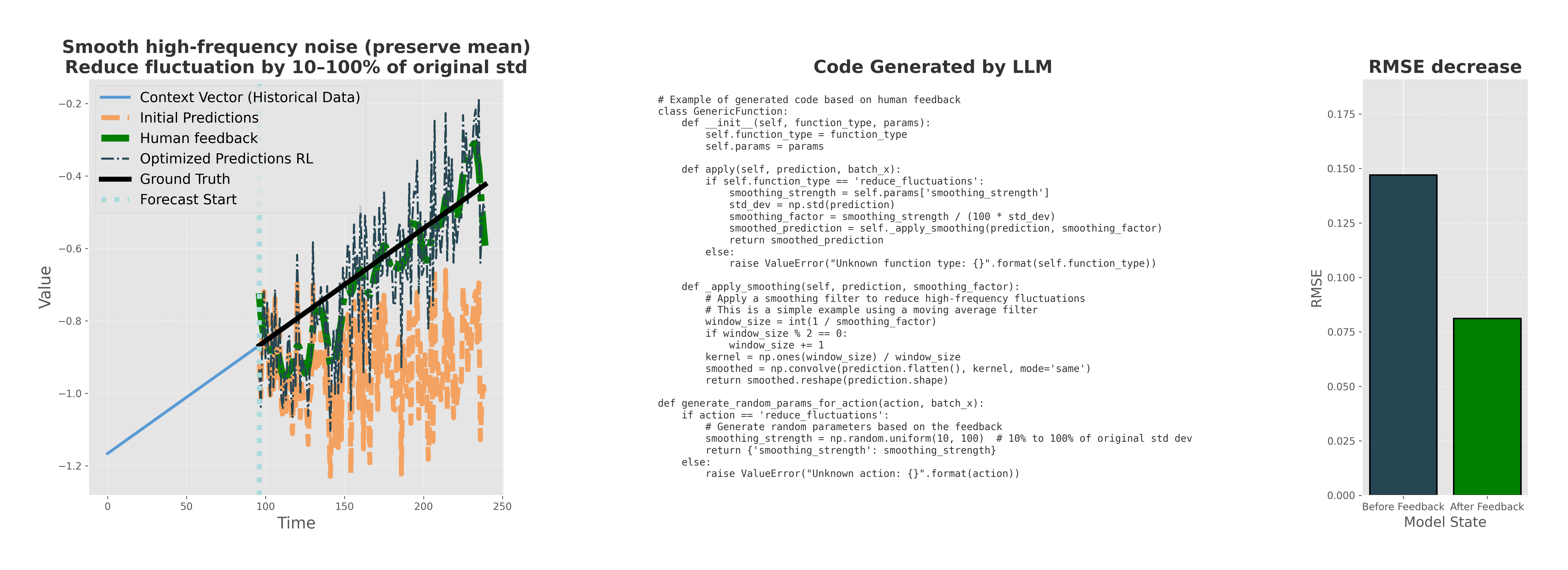
Figure 9: Human feedback integration example 1: Forecast comparison with RL and human feedback (top), code generated from human feedback (middle), and RMSE improvement (bottom). Dataset: Dominick, Model: PatchTST

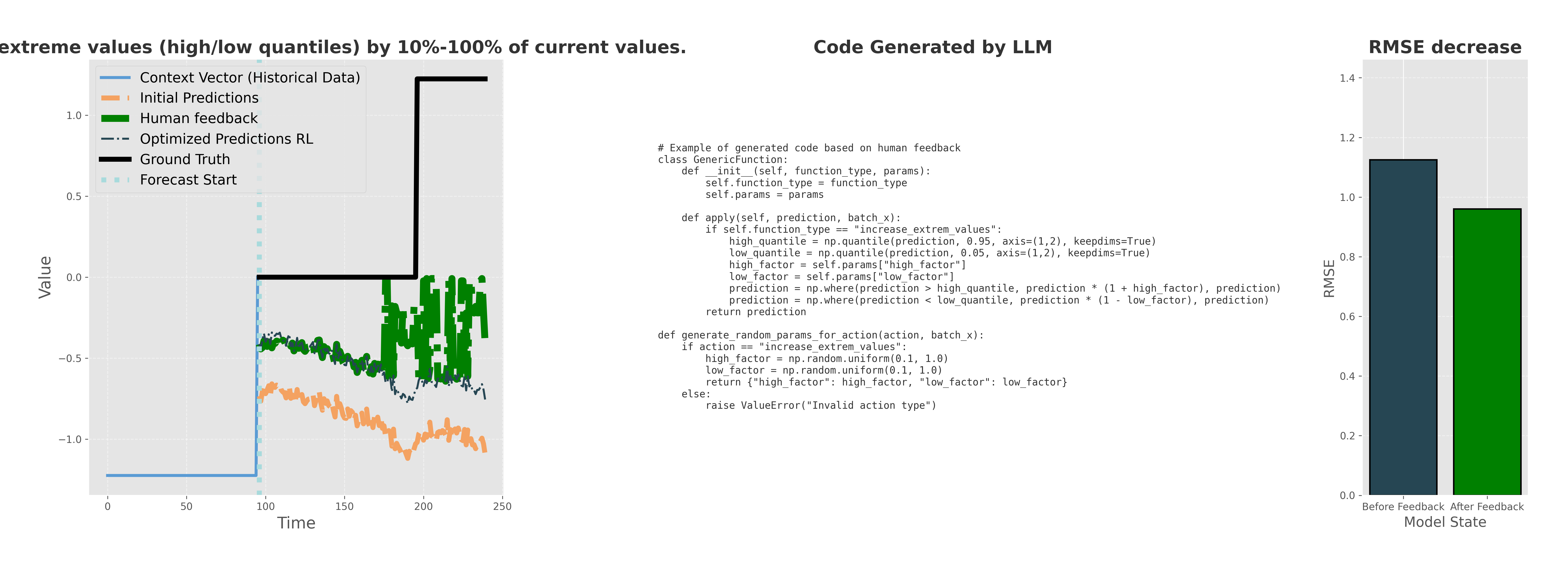
Figure 10: Human feedback integration example 2: Forecast comparison with RL and human feedback (top), code generated from human feedback (middle), and RMSE improvement (bottom). Dataset: Nature, Model: DLinear

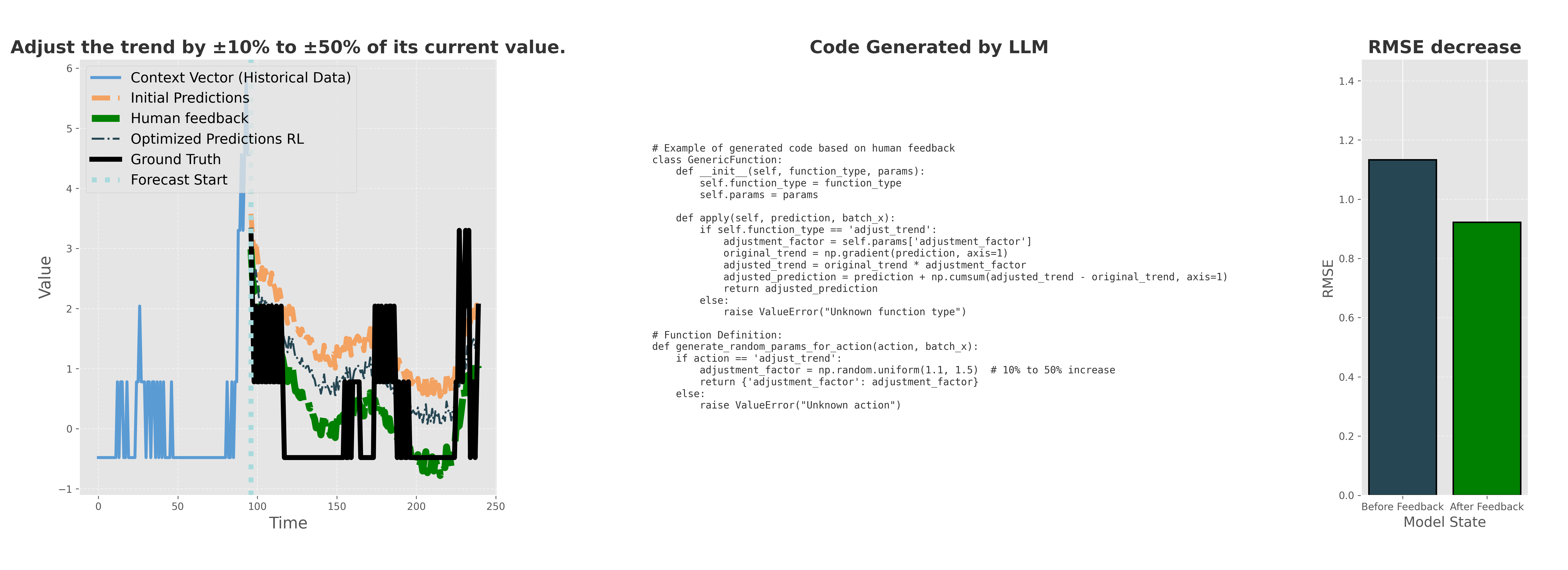
Figure 11: Human feedback integration example 3: Forecast comparison with RL and human feedback (top), code generated from human feedback (middle), and RMSE improvement (bottom). Dataset: Tourism, Model: PatchTST

6.5 Code and Reproducibility

To enable full reproducibility of our results, we provide detailed instructions for using the code associated with our framework. This section includes guidelines for setting up the environment, running the experiments, and utilizing the graphical user interface (GUI) for easy interaction with the framework. We also provide links to the repository, ensuring that interested readers can freely access and experiment with our code.

6.6 Code Usage and API Documentation

This appendix provides instructions for using the codebase and the API for time series model post-training and human feedback exploration. The framework provides a method for users to adjust model predictions using human feedback and contextual bandit algorithms, allowing the model to dynamically adapt its behavior. The code is available at https://github.com/posttraining/post_training.

Goal

The primary goal of this project is to provide an interactive environment where users can fine-tune time series model predictions based on human feedback. The framework leverages a contextual bandit approach, allowing users to explore different actions and see their impact on the model’s predictions.

Features

• Time Series Model Exploration: Train and explore various time series models with different parameters and datasets.

• Optimization Framework: Dynamically apply actions and evaluate their effects on the model’s prediction accuracy.

• Human Feedback Integration: Users can provide feedback on the predictions to improve the model’s output over time.

• Streamlit Interface: An interactive frontend for exploring and providing feedback on model predictions.

6.6.1 Examples to Use the Streamlit Application

To experiment with the Streamlit application, follow these steps:

1. Click on the following (link): Go to the webpage. You should see the configuration page as in Figure 12.

   

   Figure 12: Configuration page

2. Upload CSV File: Upload a CSV file containing the time series data. The file should be in CSV format, with rows representing different time steps and columns representing different features for multivariate datasets. A sample file, train.csv, is provided in the supplementary materials. You can see an example in Figure 13

   

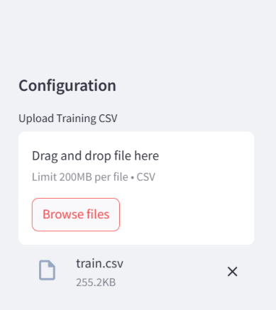
   Figure 13: Example of upload file

3. Select Model and Options: Choose the model and other options. For the model, use DLinear, as other models require a GPU to run or will take longer. The server currently supports CPU only as in Figure 14

   

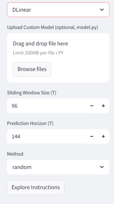
   Figure 14: Configuration Options

4. Explore Instructions: Click on the "Explore Instructions" button. After some time, you will see the optimization process (with the successful actions over the episodes) as in Figure 15

   

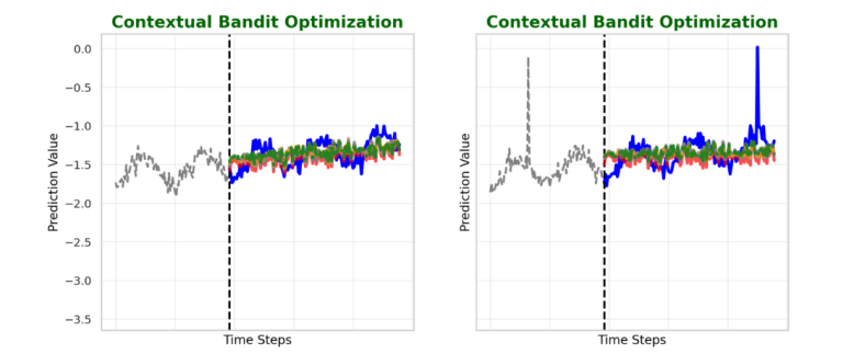
   Figure 15: Successfull and failed actions during optimization

   and the reduced MSE after each episode on the validation set as in Figure 16

   

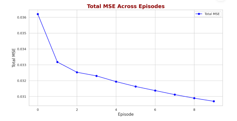
   Figure 16: MSE as function of the number of episodes

5. Provide Feedback: Enter your feedback in text, in any language. Be as descriptive as possible to guide the model. For example, you could say, "The amplitude of the predictions should be increased between 5% and 10% of the actual values." as in Figure 17

   

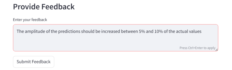
   Figure 17: Example of user prompt

6. Submit Feedback: Click on "Submit Feedback" and then "Finalize Feedback." You will see the percentage improvement and details per channel as in Figure 18

   

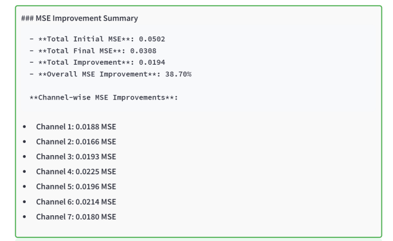
   Figure 18: Improvement Details

6.7 Installation and usage for development

Installation Instructions

Set Up the Environment

To install the required dependencies, create and activate the conda environment:

conda env create -f environment.yml

Usage

Running the Code with Command-Line Arguments

To run the post-training process and adjust the model, execute the following command:

  python main.py --train_path <path_to_train_data
--model <model_name> --window_size <window_size> --prediction_horizon <prediction_horizon>
--batch_size <batch_size> --n_samples <n_samples>

The available command-line arguments are as follows:

Argument	Description	Example
--train_path	Path to the training data CSV file	data/train.csv
--model	Name of the model to use	DLinear, PatchTST, etc.
--model_path	(Optional) Path to a custom pre-trained model	models/custom_model.py
--window_size	Sliding window size for time series	96
--prediction_horizon	Prediction horizon in terms of time steps	144
--batch_size	Batch size for training	32
--n-jobs	Number of CPU for parallel computing	1
--episodes	Number of episodes for RL training	5

Running the Streamlit App

To interact with the framework using the Streamlit interface, launch the app as follows:

streamlit run app_test.py

This will start a local server, and you can access the interface by navigating to the URL provided in the terminal.

Workflow Overview

The following steps outline the workflow of the post-training process:

1. Train the Model: Train the model using the provided training data and validate it using the validation dataset. Optionally, load a custom pre-trained model if specified.

2. Exploration Phase: After training, explore various actions on top of the model’s predictions. These actions include adjusting amplitudes, trends, or shifting values.

3. Human Feedback: Provide feedback on the predictions to guide the model towards improvements. Precise feedback, such as "increase the amplitude by 5-10%", allows the model to understand the desired adjustments.

4. Model Adaptation: Based on the feedback, the model adapts its behavior and re-tests the adjusted predictions.

5. Plotting Results: The results of the model’s predictions are visualized through plots, which are saved for further analysis.

API Documentation

The API for the framework is structured as follows:

1. app_test.py: Main script to run the Streamlit interface. Provides functionalities to explore and give feedback on model predictions.

2. contextual_bandit.py: Implements the contextual bandit logic for dynamically adjusting predictions based on feedback.

3. data_extraction.py: Contains functions for loading and preprocessing time series data.

4. llm_interaction.py: Functions for interacting with language models to interpret and apply human feedback.

5. model_extraction.py: Extracts and loads pre-trained models.

6. plot_script.py: Provides plotting utilities for visualizing predictions and feedback results.

6.8 Theoretical motivation for post training in time series forecasting

6.8.1 Problem Setup

Consider a supervised learning problem where we want to estimate a target variable $Y_{\text{true}}$ using a linear model. We assume that a ridge regression predictor $Y_{\text{\text{pred}}}$ has already been obtained, and we aim to improve its accuracy through an optimal affine correction of the form:

$$Y_{\text{corrected}}=aY_{\text{pred}}+b.$$ (3)

The goal is to determine the optimal values of $a$ and $b$ that minimize the expected mean squared error (MSE):

$$\mathcal{L}(a,b)=\mathbb{E}\left[\|Y_{\text{true}}-(aY_{\text{pred}}+b)\|^{2}\right].$$ (4)

6.8.2 Derivation of Optimal Correction Parameters

Expanding the loss function:

$$\mathcal{L}(a,b)=\mathbb{E}\left[Y_{\text{true}}^{2}-2aY_{\text{true}}Y_{\text{pred}}-2bY_{\text{true}}+a^{2}Y_{\text{pred}}^{2}+2abY_{\text{pred}}+b^{2}\right].$$ (5)

Step 1: Compute $b^{*}$ by setting $\frac{\partial\mathcal{L}}{\partial b}=0$.

$$\frac{\partial\mathcal{L}}{\partial b}=-2\mathbb{E}[Y_{\text{true}}]+2a\mathbb{E}[Y_{\text{pred}}]+2b.$$ (6)

Setting this derivative to zero and solving for $b^{*}$ gives:

$$b^{*}=\mathbb{E}[Y_{\text{true}}]-a^{*}\mathbb{E}[Y_{\text{pred}}].$$ (7)

Step 2: Compute $a^{*}$ by setting $\frac{\partial\mathcal{L}}{\partial a}=0$.

$$\frac{\partial\mathcal{L}}{\partial a}=-2\mathbb{E}[Y_{\text{true}}Y_{\text{pred}}]+2a\mathbb{E}[Y_{\text{pred}}^{2}]+2b\mathbb{E}[Y_{\text{pred}}].$$ (8)

Substituting $b^{*}$ and solving for $a^{*}$ gives:

$$a^{*}=\frac{\text{Cov}(Y_{\text{true}},Y_{\text{pred}})}{\text{Var}(Y_{\text{pred}})}.$$ (9)

Thus, the optimal correction parameters are:

$$a^{*}=\frac{\mathbb{E}[(Y_{\text{true}}-\mathbb{E}[Y_{\text{true}}])(Y_{\text{pred}}-\mathbb{E}[Y_{\text{pred}}])]}{\mathbb{E}[(Y_{\text{pred}}-\mathbb{E}[Y_{\text{pred}}])^{2}]},$$ (10)

$$b^{*}=\mathbb{E}[Y_{\text{true}}]-a^{*}\mathbb{E}[Y_{\text{pred}}].$$ (11)

6.8.3 Theoretical Risk Before and After Correction

Risk Before Correction:

The mean squared error (MSE) of the original predictor is given by:

$$R_{\text{before}}=\mathbb{E}[(Y_{\text{true}}-Y_{\text{pred}})^{2}].$$ (12)

Expanding:

$$R_{\text{before}}=\text{Var}(Y_{\text{true}})+\text{Var}(Y_{\text{pred}})-2\text{Cov}(Y_{\text{true}},Y_{\text{pred}}).$$ (13)

Risk After Correction:

The mean squared error of the optimally corrected predictor is:

$$R_{\text{after}}=\mathbb{E}[(Y_{\text{true}}-Y_{\text{corrected}})^{2}].$$ (14)

Substituting $Y_{\text{corrected}}=a^{*}Y_{\text{pred}}+b^{*}$:

$$R_{\text{after}}=\text{Var}(Y_{\text{true}})-\frac{\text{Cov}(Y_{\text{true}},Y_{\text{pred}})^{2}}{\text{Var}(Y_{\text{pred}})}.$$ (15)

6.8.4 Comparison of Risks

To understand the effect of the correction, we compute the difference:

$$R_{\text{before}}-R_{\text{after}}.$$ (16)

Substituting the expressions:

$$R_{\text{before}}-R_{\text{after}} =\left[\text{Var}(Y_{\text{true}})+\text{Var}(Y_{\text{pred}})-2\text{Cov}(Y_{\text{true}},Y_{\text{pred}})\right]$$

$$\quad-\left[\text{Var}(Y_{\text{true}})-\frac{\text{Cov}(Y_{\text{true}},Y_{\text{pred}})^{2}}{\text{Var}(Y_{\text{pred}})}\right].$$ (17)

Simplifying:

$$R_{\text{before}}-R_{\text{after}}=\text{Var}(Y_{\text{pred}})-2\text{Cov}(Y_{\text{true}},Y_{\text{pred}})+\frac{\text{Cov}(Y_{\text{true}},Y_{\text{pred}})^{2}}{\text{Var}(Y_{\text{pred}})}.$$ (18)

Rewriting using the identity:

$$\left(x-\frac{a}{x}\right)^{2}\geq 0\quad\text{for all }x>0,$$ (19)

by setting $x=\text{Var}(Y_{\text{pred}})$ and $a=\text{Cov}(Y_{\text{true}},Y_{\text{pred}})^{2}$, we obtain:

$$R_{\text{before}}-R_{\text{after}}=\left(\sqrt{\text{Var}(Y_{\text{pred}})}-\frac{\text{Cov}(Y_{\text{true}},Y_{\text{pred}})}{\sqrt{\text{Var}(Y_{\text{pred}})}}\right)^{2}.$$ (20)

Since the square of any real number is always non-negative:

$$R_{\text{before}}-R_{\text{after}}\geq 0.$$ (21)

6.8.5 Conclusion

This derivation shows that the correction always reduces the risk (or at worst, leaves it unchanged). The correction is most effective when $Y_{\text{pred}}$ is correlated with $Y_{\text{true}}$, and it does not increase the error in any case. This result shows that the correction always reduces the mean squared error.

References

- Ansari et al., (2024) Ansari, A. F., Stella, L., Turkmen, C., Zhang, X., Mercado, P., Shen, H., Shchur, O., Rangapuram, S. S., Arango, S. P., Kapoor, S., et al. (2024). Chronos: Learning the language of time series. arXiv preprint arXiv:2403.07815.
- Armstrong, (1986) Armstrong, J. S. (1986). The ombudsman: research on forecasting: A quarter-century review, 1960–1984. Interfaces, 16(1):89–109.
- Arvan et al., (2019) Arvan, M., Fahimnia, B., Reisi, M., and Siemsen, E. (2019). Integrating human judgement into quantitative forecasting methods: A review. Omega, 86:237–252.
- Bunn and Wright, (1991) Bunn, D. and Wright, G. (1991). Interaction of judgemental and statistical forecasting methods: issues & analysis. Management science, 37(5):501–518.
- Das et al., (2024) Das, A., Kong, W., Sen, R., and Zhou, Y. (2024). A decoder-only foundation model for time-series forecasting. In Forty-first International Conference on Machine Learning.
- Gardner Jr, (1985) Gardner Jr, E. S. (1985). Exponential smoothing: The state of the art. Journal of forecasting, 4(1):1–28.
- Geweke and Whiteman, (2006) Geweke, J. and Whiteman, C. (2006). Bayesian forecasting. Handbook of economic forecasting, 1:3–80.
- Girard et al., (2002) Girard, A., Rasmussen, C., Candela, J. Q., and Murray-Smith, R. (2002). Gaussian process priors with uncertain inputs application to multiple-step ahead time series forecasting. Advances in neural information processing systems, 15.
- Graves and Graves, (2012) Graves, A. and Graves, A. (2012). Long short-term memory. Supervised sequence labelling with recurrent neural networks, pages 37–45.
- Holland, (1975) Holland, J. H. (1975). Adaptation in Natural and Artificial Systems. University of Michigan Press, Ann Arbor, MI.
- Ilbert et al., (2024) Ilbert, R., Odonnat, A., Feofanov, V., Virmaux, A., Paolo, G., Palpanas, T., and Redko, I. (2024). Samformer: Unlocking the potential of transformers in time series forecasting with sharpness-aware minimization and channel-wise attention. arXiv preprint arXiv:2402.10198.
- Karnin et al., (2013) Karnin, Z. S., Koren, T., and Somekh, O. (2013). Almost optimal exploration in multi-armed bandits. In Proceedings of the 30th International Conference on Machine Learning, pages 1238–1246. PMLR.
- Kaushik et al., (2020) Kaushik, S., Choudhury, A., Sheron, P. K., Dasgupta, N., Natarajan, S., Pickett, L. A., and Dutt, V. (2020). Ai in healthcare: time-series forecasting using statistical, neural, and ensemble architectures. Frontiers in big data, 3:4.
- Khashei and Bijari, (2012) Khashei, M. and Bijari, M. (2012). A new class of hybrid models for time series forecasting. Expert Systems with Applications, 39(4):4344–4357.
- Korstanje, (2021) Korstanje, J. (2021). The sarima model. In Advanced Forecasting with Python: With State-of-the-Art-Models Including LSTMs, Facebook’s Prophet, and Amazon’s DeepAR, pages 115–122. Springer.
- Krollner et al., (2010) Krollner, B., Vanstone, B., and Finnie, G. (2010). Financial time series forecasting with machine learning techniques: A survey. In European Symposium on Artificial Neural Networks: Computational Intelligence and Machine Learning, pages 25–30.
- Kupferschmidt et al., (2022) Kupferschmidt, K. L., Skorburg, J. G., and Taylor, G. W. (2022). Delphai: A human-centered approach to time-series forecasting. In 2022 IEEE International Conference on Big Data (Big Data), pages 4014–4020. IEEE.
- Lin et al., (2023) Lin, S., Lin, W., Wu, W., Zhao, F., Mo, R., and Zhang, H. (2023). Segrnn: Segment recurrent neural network for long-term time series forecasting. arXiv preprint arXiv:2308.11200.
- (19) Liu, A., Feng, B., Xue, B., Wang, B., Wu, B., Lu, C., Zhao, C., Deng, C., Zhang, C., Ruan, C., et al. (2024a). Deepseek-v3 technical report. arXiv preprint arXiv:2412.19437.
- (20) Liu, H., Xu, S., Zhao, Z., Kong, L., Kamarthi, H., Sasanur, A. B., Sharma, M., Cui, J., Wen, Q., Zhang, C., et al. (2024b). Time-mmd: A new multi-domain multimodal dataset for time series analysis. arXiv preprint arXiv:2406.08627.
- Liu et al., (2023) Liu, Y., Hu, T., Zhang, H., Wu, H., Wang, S., Ma, L., and Long, M. (2023). itransformer: Inverted transformers are effective for time series forecasting. arXiv preprint arXiv:2310.06625.
- Madadgar et al., (2014) Madadgar, S., Moradkhani, H., and Garen, D. (2014). Towards improved post-processing of hydrologic forecast ensembles. Hydrological Processes, 28(1):104–122.
- Meisenbacher et al., (2022) Meisenbacher, S., Turowski, M., Phipps, K., Rätz, M., Müller, D., Hagenmeyer, V., and Mikut, R. (2022). Review of automated time series forecasting pipelines. Wiley Interdisciplinary Reviews: Data Mining and Knowledge Discovery, 12(6):e1475.
- Newbold, (1983) Newbold, P. (1983). Arima model building and the time series analysis approach to forecasting. Journal of forecasting, 2(1):23–35.
- Nie et al., (2023) Nie, Y., H. Nguyen, N., Sinthong, P., and Kalagnanam, J. (2023). A time series is worth 64 words: Long-term forecasting with transformers. In International Conference on Learning Representations.
- Palma et al., (2024) Palma, G., Chengalipunath, E. S. J., and Rizzo, A. (2024). Time series forecasting for energy management: Neural circuit policies (ncps) vs. long short-term memory (lstm) networks. Electronics, 13(18):3641.
- Qi et al., (2025) Qi, Y., Hu, H., Lei, D., Zhang, J., Shi, Z., Huang, Y., Chen, Z., Lin, X., and Shen, Z.-J. M. (2025). Timehf: Billion-scale time series models guided by human feedback. arXiv preprint arXiv:2501.15942.
- Qiu et al., (2024) Qiu, X., Hu, J., Zhou, L., Wu, X., Du, J., Zhang, B., Guo, C., Zhou, A., Jensen, C. S., Sheng, Z., and Yang, B. (2024). Tfb: Towards comprehensive and fair benchmarking of time series forecasting methods. Proc. VLDB Endow., 17:2363 – 2377.
- Rasul et al., (2023) Rasul, K., Ashok, A., Williams, A. R., Ghonia, H., Bhagwatkar, R., Khorasani, A., Bayazi, M. J. D., Adamopoulos, G., Riachi, R., Hassen, N., et al. (2023). Lag-llama: Towards foundation models for probabilistic time series forecasting. arXiv preprint arXiv:2310.08278.
- Sampson, (1976) Sampson, J. R. (1976). Adaptation in natural and artificial systems (john h. holland).
- Schulman et al., (2017) Schulman, J., Wolski, F., Dhariwal, P., Radford, A., and Klimov, O. (2017). Proximal policy optimization algorithms. arXiv preprint arXiv:1707.06347.
- Tavenard et al., (2020) Tavenard, R., Faouzi, J., Vandewiele, G., Divo, F., Androz, G., Holtz, C., Payne, M., Yurchak, R., Rußwurm, M., Kolar, K., et al. (2020). Tslearn, a machine learning toolkit for time series data. Journal of machine learning research, 21(118):1–6.
- Verkade et al., (2013) Verkade, J., Brown, J., Reggiani, P., and Weerts, A. (2013). Post-processing ecmwf precipitation and temperature ensemble reforecasts for operational hydrologic forecasting at various spatial scales. Journal of Hydrology, 501:73–91.
- Webby and O’Connor, (1996) Webby, R. and O’Connor, M. (1996). Judgemental and statistical time series forecasting: a review of the literature. International Journal of forecasting, 12(1):91–118.
- Wu et al., (2021) Wu, H., Xu, J., Wang, J., and Long, M. (2021). Autoformer: Decomposition transformers with auto-correlation for long-term series forecasting. Advances in neural information processing systems, 34:22419–22430.
- Zeng et al., (2023) Zeng, A., Chen, M., Zhang, L., and Xu, Q. (2023). Are transformers effective for time series forecasting? In Proceedings of the AAAI conference on artificial intelligence, volume 37, pages 11121–11128.
- Zhang and Yan, (2023) Zhang, Y. and Yan, J. (2023). Crossformer: Transformer utilizing cross-dimension dependency for multivariate time series forecasting. In The eleventh international conference on learning representations.
- Zhou et al., (2021) Zhou, H., Zhang, S., Peng, J., Zhang, S., Li, J., Xiong, H., and Zhang, W. (2021). Informer: Beyond efficient transformer for long sequence time-series forecasting. In Proceedings of the AAAI conference on artificial intelligence, volume 35, pages 11106–11115.
- Zhou, (2020) Zhou, Y. (2020). Real-time probabilistic forecasting of river water quality under data missing situation: Deep learning plus post-processing techniques. Journal of Hydrology, 589:125164.