IFT-UAM/CSIC-25-050
May 20^th, 2025

It has recently been shown that one can derive consistent thermodynamical expressions in the Lorentzian Taub–NUT spacetime keeping the Misner-string singularities and taking into account their contributions in the Komar integrals. We show how the same results are obtained when the Mister-string singularities are removed by using Misner’s procedure because, even though the complete spacetime has no such singularities anymore, they are unavoidable in all spacelike hypersurfaces which are used in the Komar integrals. Different choices of hypersurfaces may contain different strings and lead to different physics, though.

1. Introduction. The Lorentzian Taub-NUT solution of the vacuum Einstein equations [1, 2] can be seen as a relatively simple generalization of the Schwarzschild solution of mass $M$ that includes a new parameter, the NUT charge $N$, that can be interpreted as a “magnetic mass” (if we view the standard ADM mass as the “electric mass”). This solution can be written in the form

$$ds^{2}=\lambda(r)(dt+A)^{2}-\lambda^{-1}(r)dr^{2}-\left(r^{2}+N^{2}\right)d\Omega_{(2)}^{2}\,,$$ (1)

where

$$\lambda(r) =\frac{(r-r_{+})(r-r_{-})}{r^{2}+N^{2}}\,,$$ (2a)

$$A =2N\cos{\theta}\,d\varphi\,,$$ (2b)

$$d\Omega_{(2)}^{2} =d\theta^{2}+\sin^{2}{\theta}d\varphi^{2}\,,$$ (2c)

and where we have defined

$$r_{\pm}=M\pm r_{0}\,,\hskip 28.45274ptr_{0}^{2}=M^{2}+N^{2}.$$ (3)

The presence of this intriguing parameter is one of the most interesting aspects of this solution. The parallelism between the NUT charge and the magnetic charge of the Dirac monopole is reinforced by the presence of Misner-string singularities in the Taub-NUT solution, which bear a strong similarity to the Dirac-string singularities of the electromagnetic field of the Dirac magnetic monopole [3], as we are going to see.

First of all, notice that the the 1-form $A$ of the Taub–NUT solution Eq. (2b) is identical to the field of the Dirac monopole in some gauge. Coordinate transformations of the form

$$t\to t+\chi(x)\,,\hskip 28.45274pt\partial_{t}\chi=0\,,$$ (4)

are equivalent to transformations of $A$ of the form

$$A\to A+d\chi\,,$$ (5)

and to gauge transformations of the Dirac monopole field. In order to see where the string singularities lie, it is convenient to perform a gauge transformation $t\to t+2Ns\varphi$, where the parameter $s$ can take the values $-1,0,+1$. The 1-form $A$ takes the form

$$A=2N(\cos{\theta}+s)\,d\varphi\,,$$ (6)

or

$$A=2N(\cos{\theta}+s)\,d\varphi=2N\frac{z+sr}{r(r^{2}-z^{2})}(xdy-ydx)\,,$$ (7)

in Cartesian coordinates. The denominator goes to zero quadratically at $r=|z|$, (the whole $z$ axis, $x=y=0$). Thus, the 1-form will have a singularity when $z+s|z|\neq 0$, that is

$$s =0\,,\hskip 28.45274pt z$$ the whole axis (8)

$$s =+1\,,\hskip 28.45274pt z>0$$ the semiaxis

$$s =-1\,,\hskip 28.45274pt z<0$$ the semiaxis

These singularities of the electromagnetic field are the Dirac strings. For different values of $s$ we obtain different field configurations of the electromagnetic field. They are related by large gauge transformations that modify the asymptotic behaviour and, therefore, cannot be seen as physically equivalent. However, since they should be undetectable by electrically charged particles whose charges obey the Dirac quantization condition [3], they have long been considered unphysical. The fact that, as we are going to see, one can obtain stringless solutions with similar properties [4] seems to support this point of view.

In the case of the Taub–NUT metric, we find something similar: after performing the above transformation (now, a general coordinate transformation), we find that

$$g^{tt}=\frac{1}{\lambda}-\frac{4N^{2}(\cos\theta+s)^{2}}{(r^{2}+N^{2})\sin^{2}\theta}\,,$$ (9)

and

$$\frac{(\cos{\theta}+s)^{2}}{\sin^{2}{\theta}}=\left\{\begin{array}[]{lll}\cot^{2}{\theta}\,,&\text{for $s=0$,}&\text{singular at $\theta=0,\pi\Rightarrow\forall z$}\\ \cot^{2}{(\theta/2)}\,,&\text{for $s=+1$,}&\text{singular at $\theta=0\Rightarrow z>0$}\\ \tan^{2}{(\theta/2)}\,,&\text{for $s=-1$,}&\text{singular at $\theta=\pi\Rightarrow z<0$}\end{array}\right.$$ (10)

Misner showed in Ref. [5] that one can construct a solution in which these singularities are absent by using in the $z>0$ region a Taub–NUT solution whose Misner string lies in the negative $z$-axis ($s=-1$)

$$ds^{2}=\lambda(r)\left[dt^{(+)}+2N(\cos{\theta}-1)\,d\varphi\right]^{2}-\lambda^{-1}(r)dr^{2}-\left(r^{2}+N^{2}\right)d\Omega_{(2)}^{2}\,,$$ (11)

in the $z<0$ region, a Taub–NUT solution whose Misner string lies in the positive $z$-axis ($s=+1$),

$$ds^{2}=\lambda(r)\left[dt^{(-)}+2N(\cos{\theta}+1)\,d\varphi\right]^{2}-\lambda^{-1}(r)dr^{2}-\left(r^{2}+N^{2}\right)d\Omega_{(2)}^{2}\,,$$ (12)

and gluing them across the equatorial plane $z=0$, i.e. relating them by a coordinate transformation in the overlap:

$$t^{(+)}=t^{(-)}+4N\varphi\,,$$ (13)

Since the period of the angular coordinate $\varphi$ is $2\pi$ and we must identify $\varphi\sim\varphi+2\pi$, the time coordinate in both patches must also be periodic with period $8\pi N$

$$t^{(\pm)}\sim t^{(\pm)}+8\pi N.$$ (14)

In the resulting solution, the time coordinate parametrizes a S¹ which is non-trivially fibered over the S² parametrized by the coordinates $\theta$ and $\varphi$ at each value of the radial coordinate $r$. The new solution is locally identical to the stringless regions of the original Taub–NUT solution Eq. (1). The information contained in the missing Misner strings is now contained in the non-trivial topology.

In Ref. [4] Wu and Yang showed how to construct a non-trivial U$(1)$ ($\sim$ S¹) bundle over S² locally identical to the stringless regions of the Dirac magnetic monopole. This construction is essentially identical to Misner’s.

Evidently, the periodic identification of the time coordinate comes with its own problems, like the presence of closed timelike curves, to start with. Another problem of special interest to us is that the Wick-rotated solution has a conical singularity at the location of the event horizon $r=r_{+}$ unless the Euclidean time has a period of $\beta=2\pi/\kappa$, $\kappa$ being the horizon’s surface gravity. The consistency condition $\beta=8\pi N$ constrains the parameter space of the solution, leaving us with a single free parameter and leading to the loss of full cohomogeneity in the first law of black-hole thermodynamics obtained through the Euclidean approach.

In Refs. [6, 7] it was shown that, perhaps, there is no need to remove the Misner-string singularities because they are rather mild and the spacetime is geodesically complete (the singularities are transparent for free-falling observers) and essentially free of causal pathologies. If the strings are kept, the problems that arise in the Euclidean approach to black-hole thermodynamics disappear [8] and one can recover the same results in the Lorentzian setting if one takes into account the contributions of the strings [9].

2. The Lorentzian approach to Taub–NUT thermodynamics. In the Lorentzian approach to black-hole thermodynamics both the Smarr formula and the first law can be derived by integrating the exterior derivatives of certain on-shell closed 2-forms over spacelike hypersurfaces with two boundaries: one at a section of the horizon (usually the bifurcation sphere $\mathcal{BH}$) and the 2-sphere at spatial infinity S${}^{2}_{\infty}$. Stokes theorem leads to an identity relating the integrals of the 2-forms at both boundaries which becomes the Smarr formula [10, 11] or the first law [12].

The 2-form whose (vanishing) exterior derivative one has to integrate in order to obtain the Smarr formula is the Komar charge [13] (General Relativity without matter) or generalizations thereof [14, 15, 16] associated to the Killing vector $k$ that becomes null over the event horizon, $\mathbf{K}[k]$. If $\Sigma^{3}$ is a spacelike hypersurface such that $\partial\Sigma^{3}=\mathcal{BH}\cup$S${}^{2}_{\infty}$, taking into account the different orientation of these two boundaries

$$0=\int_{\Sigma^{3}}d\mathbf{K}[k]=\int_{\mathcal{BH}}\mathbf{K}[k]-\int_{\text{S}^{2}_{\infty}}\mathbf{K}[k]\,.$$ (15)

The integral at infinity can be expressed in terms of conserved charges, which are defined asymptotically, while the integral over the bifurcation sphere can be expressed in terms of properties of the horizon: temperature, entropy, potentials etc. The identity of these two results is the Smarr formula.

In the case of the Taub–NUT solution with Misner strings, the boundary of the spacelike surface $\Sigma^{3}$ contains one additional boundary per string and

$$0=\int_{\Sigma^{3}}d\mathbf{K}[k]=\int_{\mathcal{BH}}\mathbf{K}[k]-\int_{\text{S}^{2}_{\infty}}\mathbf{K}[k]+\sum_{\rm strings}\int_{\rm string}\mathbf{K}[k]\,.$$ (16)

In practice (see Fig 1) the integrals over the strings are computed as integrals over cones (surfaces of fixed $t$ and $\theta$ are actually cones rather than tubes) from $r=r_{+}$ (the horizon) to some finite value of $r$, the integral over the bifurcation sphere now must exclude the regions inside the cones that surround the intersection between the strings and the sphere and the integral over the sphere at infinity is computed as an integral over a sphere of finite radius $r$ excluding the regions that surround the intersection between the strings and the sphere. Then, the final result is obtained by taking the limits $r\to\infty$ and $\epsilon\to 0$.

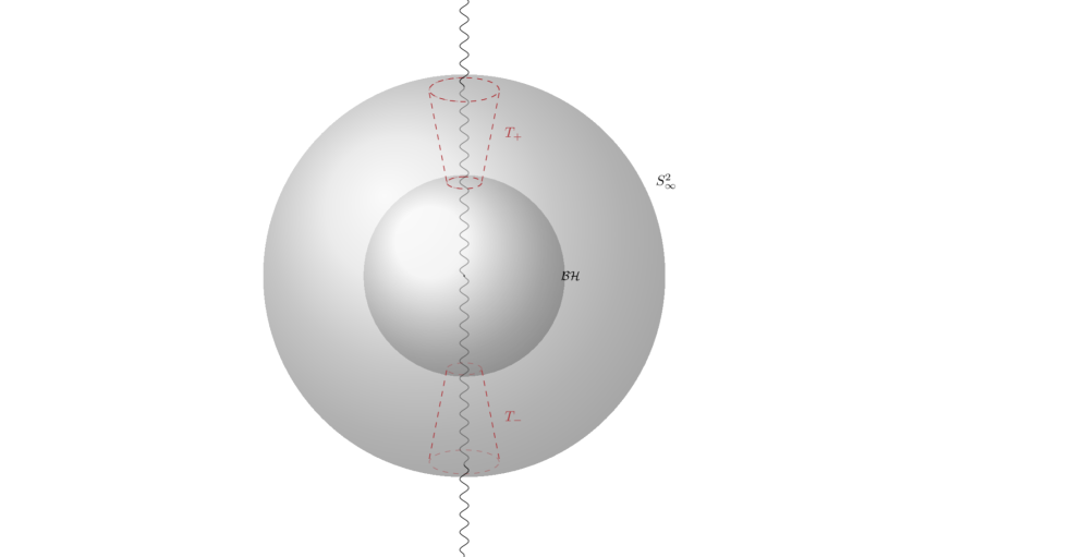
Figure 1: This figure represents schematically the region over which we integrate $d\mathbf{K}[k]$, i.e. the region contained inside the boundaries S${}^{2}_{\infty}$ (the 2-sphere at spatial infinity), $\mathcal{BH}$ (the bifurcation sphere) and the two cones T₊ and T_- surrounding the Misner-string singularities (when they are present).

The first two integrals in the above expression give usual results:

$$\int_{\mathcal{BH}}\mathbf{K}[k] =ST\,,$$ (17a)

$$\int_{\text{S}^{2}_{\infty}}\mathbf{K}[k] =M/2\,,$$ (17b)

where $S$ is the Bekenstein–Hawking entropy ($A/4G_{N}^{(4)}$, where $A$ is the area of any section of the horizon), $T$ is the temperature ($\kappa/(2\pi)$ where $\kappa$ is the surface gravity of the horizon) and $M$ is the ADM mass. There is dependence on the NUT charge hidden in $S$ and $T$ and the standard Smarr formula $M=2ST$ is not satisfied.

The integrals over the strings in the $z>0$ and $z<0$ regions provide the missing terms and can be written in the form

$$\int_{\text{string}_{\pm}}\mathbf{K}[k]=\psi_{\pm}\mathcal{N}_{\pm}\,,$$ (18)

where $\psi_{\pm}$ play the role of chemical potentials and coincide with the surface gravities of the strings and $\mathcal{N}_{\pm}$, the thermodynamical variables conjugate to them, are related but not equal to the NUT charge $N$.

With these additional contributions, the Smarr formula takes the general form [9]

$$M=2\left(TS+\psi_{+}\mathcal{N}_{+}+\psi_{-}\mathcal{N}_{-}\right)\,,$$ (19)

and it is identically satisfied by the Taub–NUT solutions with $s=\pm 1,0$, for which $\mathcal{N}_{\mp}=0$ and $\mathcal{N}_{\pm}\neq 0$, respectively.

3. The Lorentzian approach to the stringless Taub–NUT spacetime. What happens when one uses Misner’s construction to remove the string singularities? The Komar integrals associated to the strings no longer contribute to the Smarr formula but one may expect the integrals over the spheres to give additional contributions owing to the fact that they have to be computed for the northern ($z>0$) and southern hemispheres ($z<0$) separately, but it can be seen by direct calculation that this expectation is not fulfilled and one apparently gets the inconsistent result $M=2ST$.

At this point we should remember that we must integrate $d\mathbf{K}[k]\doteqdot 0$ over a spacelike hypersurface ($t=0$, say) and we must pay attention to the definition of this hypersurface in the stringless spacetime, which has two coordinate patches and two time coordinates. The choice $t^{(+)}=0$ implies, according to Eq. (13), $t^{(-)}=-4N\varphi$ and the induced metric of the hypersurface in both hemispheres is the same metric one gets by setting $t=0$ in the solution

$$ds^{2}=\lambda(r)\left[dt+2N(\cos{\theta}-1)\,d\varphi\right]^{2}-\lambda^{-1}(r)dr^{2}-\left(r^{2}+N^{2}\right)d\Omega_{(2)}^{2}\,,$$ (20)

which has a Misner-string singularity in the $z<0$ axis.

In the same way, we find a Misner-string singularity along the $z>0$ semiaxis in the hypersurface defined by $t^{(-)}=0$ ($t^{(+)}=4N\varphi$) and, in the hypersurface $t^{(+)}=2N\varphi$ ($t^{(-)}=-2N\varphi$), there is a Misner-string singularity along both semiaxes. These three choices of spacelike hypersurfaces are obviously related to the three values of $s$ we have considered here, although there can be more.

Thus, although the stringless Taub–NUT solution is completely regular outside the horizon, its spacelike hypersurfaces exhibit Misner-string singularities that must be taken into account exactly in the same fashion they are taken into account when the singularities are present in the full solution. Thus, integrating $d\mathbf{K}[k]\doteqdot 0$ over these hypersurfaces one has to do exactly the same calculations as in Ref. [9] and one gets results that fit in the general Smarr formula Eq. (19). There is, however an important difference: in the solutions with Misner-string singularities one gets different values of the charges and potentials for different values of $s$. This is acceptable because they are physically inequivalent solutions with different string singularities. However, obtaining different values for different choices of hypersurface in the globally regular, stringless solution indicates that these hypersurfaces are physically inequivalent and observers associated to them will experience different physical phenomena.

The Euclidean approach does not make use of hypersurfaces and the Misner-string singularities associated to them seem to be totally absent. The problems found in the thermodynamical description of the stringless Taub–NUT solution are unaffected by our observations.

Acknowledgments The authors would like to thank R. Hennigar for reading the manuscript and useful comments. The work of GB, CG-F, TO and JLVC has been supported in part by the MCI, AEI, FEDER (UE) grants PID2021-125700NB-C21 (“Gravity, Supergravity and Superstrings” (GRASS)) and IFT Centro de Excelencia Severo Ochoa CEX2020-001007-S. The work of GB has been supported by the fellowship CEX2020-001007-S-20-5. The work of CG-F was supported by the MU grant FPU21/02222. The work of JLVC has been supported by the CSIC JAE-INTRO grant JAEINT-24-02806. TO wishes to thank M.M. Fernández for her permanent support.

References

- [1] A. H. Taub, “Empty space-times admitting a three parameter group of motions,” Annals Math. 53 (1951), 472-490 DOI:10.2307/1969567
- [2] E. Newman, L. Tamburino and T. Unti, “Empty space generalization of the Schwarzschild metric,” J. Math. Phys. 4 (1963), 915 DOI:10.1063/1.1704018
- [3] P. A. M. Dirac, “Quantised singularities in the electromagnetic field,,” Proc. Roy. Soc. Lond. A 133 (1931) no.821, 60-72 DOI:10.1098/rspa.1931.0130
- [4] T. T. Wu and C. N. Yang, “Concept of Nonintegrable Phase Factors and Global Formulation of Gauge Fields,” Phys. Rev. D 12 (1975), 3845-3857 DOI:10.1103/PhysRevD.12.3845
- [5] C. W. Misner, “The Flatter regions of Newman, Unti and Tamburino’s generalized Schwarzschild space,” J. Math. Phys. 4 (1963), 924-938 DOI:10.1063/1.1704019
- [6] G. Clément, D. Gal’tsov and M. Guenouche, “Rehabilitating space-times with NUTs,” Phys. Lett. B 750 (2015), 591-594 DOI:10.1016/j.physletb.2015.09.074 [arXiv:1508.07622 [hep-th]].
- [7] G. Clément and M. Guenouche, “Motion of charged particles in a NUTty Einstein-Maxwell spacetime and causality violation,” Gen. Rel. Grav. 50 (2018) no.6, 60 DOI:10.1007/s10714-018-2388-y [arXiv:1606.08457 [gr-qc]].
- [8] R. A. Hennigar, D. Kubizňák and R. B. Mann, “Thermodynamics of Lorentzian Taub-NUT spacetimes,” Phys. Rev. D 100 (2019) no.6, 064055 DOI:10.1103/PhysRevD.100.064055 [arXiv:1903.08668 [hep-th]].
- [9] A. B. Bordo, F. Gray, R. A. Hennigar and D. Kubizňák, “Misner Gravitational Charges and Variable String Strengths,” Class. Quant. Grav. 36 (2019) no.19, 194001 DOI:10.1088/1361-6382/ab3d4d [arXiv:1905.03785 [hep-th]].
- [10] J. M. Bardeen, B. Carter and S. W. Hawking, “The Four laws of black hole mechanics,” Commun. Math. Phys. 31 (1973), 161-170 DOI:10.1007/BF01645742
- [11] B. Carter, “Black holes equilibrium states,” Contribution to: Les Houches Summer School of Theoretical Physics, 57-214.
- [12] R. M. Wald, “Black hole entropy is the Noether charge,” Phys. Rev. D 48 (1993) no.8, R3427. DOI:10.1103/PhysRevD.48.R3427 [gr-qc/9307038].
- [13] A. Komar, “Covariant conservation laws in general relativity,” Phys. Rev. 113 (1959), 934-936 DOI:10.1103/PhysRev.113.934
- [14] A. Magnon, “On Komar integrals in asymptotically anti-de Sitter space-times,” J. Math. Phys. 26 (1985), 3112-3117 DOI:10.1063/1.526690
- [15] S. L. Bazanski and P. Zyla, “A Gauss type law for gravity with a cosmological constant,” Gen. Rel. Grav. 22 (1990), 379-387
- [16] D. Kastor, S. Ray and J. Traschen, “Smarr Formula and an Extended First Law for Lovelock Gravity,” Class. Quant. Grav. 27 (2010), 235014 DOI:10.1088/0264-9381/27/23/235014 [arXiv:1005.5053 [hep-th]].
- [17] R. Ballesteros and T. Ortín, “Generalized Komar charges and Smarr formulas for black holes and boson stars,” [arXiv:2409.08268 [gr-qc]] (to be published in SciPost Core).
- [18] G. Barnich and F. Brandt, “Covariant theory of asymptotic symmetries, conservation laws and central charges,” Nucl. Phys. B 633 (2002), 3-82 DOI:10.1016/S0550-3213(02)00251-1 [hep-th/0111246 [hep-th]].
- [19] G. Barnich, “Boundary charges in gauge theories: Using Stokes theorem in the bulk,” Class. Quant. Grav. 20 (2003), 3685-3698 DOI:10.1088/0264-9381/20/16/310 [hep-th/0301039 [hep-th]].