22institutetext: International Laboratory of Stochastic Analysis and its Applications,
HSE University, Moscow, Russia
33institutetext: Faculty of Applied Mathematics, Physics and Information Technologies,
Chuvash State University, Cheboksary, Russia
44institutetext: ITMO university, St. Petersburg, Russia
Liquidity provision with -reset strategies:
a dynamic historical liquidity approach
Abstract
Since the launch of Uniswap and other AMM protocols, the DeFi industry has evolved from simple constant product functions with uniform liquidity distribution across the entire price axis to more advanced mechanisms that allow Liquidity Providers (LPs) to concentrate capital within selected price ranges. This evolution has introduced new research challenges focused on optimizing capital allocation in Decentralized Exchanges (DEXs) under dynamic market conditions. In this paper, we present a methodology for finding optimal liquidity provision strategies in DEXs within a specific family of -reset strategies. The approach is detailed step by step and includes an original method for approximating historical liquidity within active pool ranges using a parametric model that does not rely on historical liquidity data. We find optimal LP strategies using a machine learning approach, evaluate performance over an out-of-time period, and compare the resulting strategies against a uniform benchmark. All experiments were conducted using a custom backtesting framework specifically developed for Concentrated Liquidity Market Makers (CLMMs). The effectiveness and flexibility of the proposed methodology are demonstrated across various Uniswap v3 trading pairs, and also benchmarked against an alternative backtesting and strategy development tool.
Keywords:
Decentralized exchange Automated market-making Liquidity provision Uniswap Decentralized finance Blockchain.1 Introduction
Decentralized Finance (DeFi) has become one of the fastest-growing areas of the blockchain industry, offering an open, programmable architecture to create, execute, and automate financial services through smart contracts, which are self-executing programs that run on-chain without intermediaries [1]. A central component of this ecosystem is the Decentralized Exchange (DEX), which is based on the Automated Market Maker (AMM) mechanism. In an AMM, liquidity is pooled and trading prices are set algorithmically rather than through a traditional order book. Since the launch of Uniswap V1/V2 [2], such protocols have provided a simple and accessible trading model in which pricing is governed by a predefined mathematical rule, most notably the constant product function [3].
Despite their elegance and novelty, early AMM protocols suffered from capital inefficiency: liquidity was distributed uniformly across the entire price axis, although most trading activity occurred within a relatively narrow range. Uniswap V3 addressed this shortcoming by introducing the Concentrated Liquidity Market Maker (CLMM) concept [4], which allows liquidity providers (LP) to allocate capital to selected price intervals. Under CLMM, an LP earns fees only when the pool price is within the chosen range, turning liquidity provision from a passive activity into an active management problem that requires continuous monitoring of market conditions [5].
Consequently, optimal liquidity provision has become a critical research objective. Active liquidity management requires LPs to make decisions that weigh current and expected market conditions, risk exposure, and competition within pools. Therefore, designing effective liquidity management strategies requires a deep analysis of pool dynamics and the development of specialized tools to test research hypotheses.
This paper introduces a general methodology for developing models that support optimal liquidity provision decisions on CLMM platforms. At the core of the approach is a custom-designed backtesting framework that approximates historical liquidity from pool swap data, eliminating the need for historical in-range liquidity data. The resulting tool is lightweight, scalable, and suitable not only for LP strategies but also for analyzing prospective AMM designs. The methodology comprises:
-
•
Approximating historical liquidity within the active ranges of the pool.
-
•
Formalizing the LP reward optimization problem.
-
•
Training machine learning models with market features.
-
•
Evaluating the models on an out-of-time period and comparing to a uniform benchmark strategy.
-
•
Benchmark comparison against an alternative DeFi backtesting and strategy development tool.
The remainder of the paper is organized as follows. Section 2 formalizes the problem and describes key concepts, strategy structure, overall ML architecture, and reward modeling techniques. Section 3 reviews related work. Section 4 presents an empirical study of historical Uniswap V3 pool data, covering liquidity reconstruction, model training, and performance evaluation. Section 5 summarizes the findings and provides directions for future research.
2 Background and Proposed Solution
This section presents a methodology for determining the optimal liquidity provision strategy using historical data analysis. The overall approach is based on modeling the processes inside a liquidity pool and involves the following consecutive stages: (i) modeling pool dynamics over a historical period, (ii) identifying the optimal LP strategies, and (iii) developing and testing an ML model for future decision making. Practical results, modeling details of the ML implementation, and a comparison with an alternative toolkit are given in Section 4.
To answer the question of what the optimal strategy should be in real time under current market conditions, the abstract ML model must be trained on historical data. The market state at each capital allocation moment is described by a set of characteristics (features), and the target variables are vectors of optimal capital shares in the pool price ranges. The vector of optimal capital shares constitutes the historical optimal strategy. Determining such an optimal strategy requires a strictly formalized methodology that integrates conceptual, architectural, and mathematical tools. We present the complete methodology, including the main concepts and research tools utilized in this work.
2.1 Key Concepts and External Data
2.1.1 Prices.
After choosing the trading pair (e.g. USDC/ETH†††In this research, ETH denotes Wrapped ETH (WETH) — the ERC-20 tokenized version of Ether that is used for interacting with AMM protocols.) and the specific DEX pool with a given fee tier for which the optimal liquidity model will be constructed, we select a historical time interval—the modeling period—over which the simulation is carried out. Next, we extract the set of swap transactions executed in the selected pool during this period and reconstruct the in-pool prices from those swaps. The resulting set of historical prices is denoted . Price intervals that contain elements of are referred to as active (or working) ranges.
The first task to address before looking for optimal LP strategies is to model the historical fee rewards of the pool within the active ranges. In our framework, relying on aggregated minute-, hour-, or day-level price data is inadequate: precise modeling requires the full sequence of in-pool price updates generated by every swap during the modeling period, together with the corresponding trade volumes. With the assumed fixed liquidity across the pool ranges, any price movement implies a change in the token reserves held in the active ranges, driven by traders who swap one pool token for the other. Given the volumes required to move the price in the pool along the set under the fee tier , we compute the fees paid by the pool for the liquidity supplied by LPs within the active ranges. Because trades within the pool are bidirectional, using aggregated data may omit part of the flow that actually passes through the pool and, at a structural level, misstate the modeled fee income.
2.1.2 Volumes and TVL.
Each swap is associated with a trade volume, which we express in the chosen numéraire and use as a historical benchmark to approximate the historical liquidity of the pool. We refer to these as historical volumes and denote them by . The average total value locked in the pool (TVL) during the modeling period is denoted by ; this quantity is required to recover the level of liquidity within the active ranges.
It is worth highlighting that the quantity does not require an overly rigid estimation procedure. If, for any reason, the average TVL during the modeling period cannot be reliably assessed, one can simply fix to the TVL of the pool observed at the beginning of the study. The historical reward modeling technique proposed in [6] approximates the liquidity profile by benchmarking against the historical fee income of the pool. In this case, the modeled trade volumes that determine the modeled reward levels of the pool pass through the pool’s local price zone bounded by active historical ranges. This implies that the overall approximated form of the pool’s historical liquidity is less important to us than the specific configuration of the local zone containing active ranges. Consequently, using an approximate level of TVL for is admissible, since the algorithm dynamically approximates the liquidity levels within the working ranges.
2.2 Baseline Strategy Type
The baseline strategy considered in this study is the dynamic -reset strategy with symmetric shape. Building on the exposition in [5], the mechanism is described in detail in [6]; we summarize it here for completeness.
2.2.1 Bucket partition.
Before the strategy is applied, the price axis is partitioned into contiguous buckets of equal width, creating a set . Bucket is delimited by a lower and an upper price, and , such that for . Adjacency is enforced at the boundaries of the buckets: for and for . Each bucket has the same fixed width .
There is no universal rule for selecting . The researcher chooses the partitioning rule, namely the boundary prices and with the parameter so that the entire set of active ranges in the modeling period will be covered by , while ensuring that the width of the bucket is not smaller than the minimum tick size of the pool. It is essential that both the width and the strategy parameter remain fixed during model training and subsequent deployment.
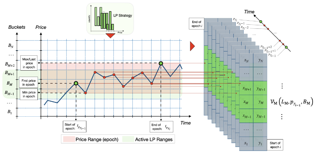
2.2.2 Strategy algorithm.
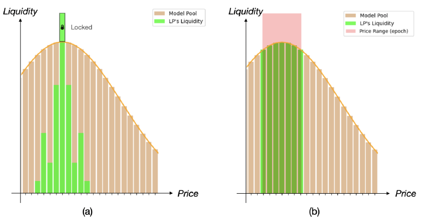
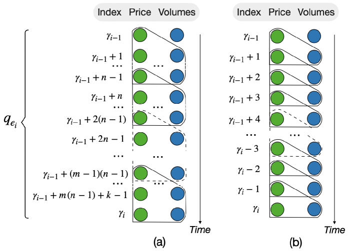
At the moment that the LP allocates capital to the pool as liquidity , as in [5] we identify reference bucket with the index that contains the initial price . The parameter is then fixed: It specifies how many buckets on either side of the reference bucket will also receive LP liquidity. These buckets (and their associated price ranges) are called the LP-liquid buckets and are denoted by set with size . The core rebalancing rule is as follows: If the next observed price falls into a bucket with index where , the reference index is updated and the liquidity of the LP is reallocated to the new set of buckets, as illustrated in Fig. 1.
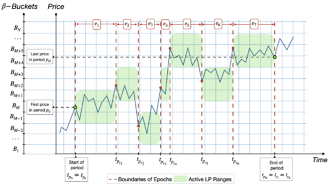
The instants at which liquidity is reallocated, that is, when the price exits the current set of liquid buckets from LP, are called reset moments or epoch switches. An epoch is the time interval during which the reference bucket index remains fixed within the modeling period. The total number of epochs is fully determined by the width of the bucket and the parameter for a given price set ; in live trading, the length of an epoch is a random variable. The minimum value on historical data arises when the initial set chosen at already covers every price in , so no reallocation occurs except for closing the position at the end of the period. Let the set of epochs be . For , each epoch corresponds to a subset of prices from ; collectively, these form
| (1) |
where denotes the index of the price at which the -th epoch ends, with and . The size of an epoch can be quantified in two ways. First, as the time difference between the two reset instants that bracket the epoch, , and second, as the number of price observations it contains, . We regard the last price of the current epoch as the first price of the next one, thereby assuming a minimum latency for allocation decision making in one block. When the position is closed at the end of the modeling period, a corner case can occur in which an epoch contains only one price, i.e. . We classify such an epoch as degenerate and at the same time the epoch size as . Denote , as the vectors of epoch sizes expressed, respectively, in units of elapsed time and in counts of price updates; both notions of size are used in the remainder of the paper.
2.3 Concept of Liquidity
We have already introduced the concept of LP-liquid buckets and spoken of deploying LP capital within price ranges "as liquidity". In this subsection, we formalize the term and outline how liquidity is computed. In the Uniswap family of protocols, the constant (historically denoted ) from the constant product function plays a central role in both the original AMM and its concentrated-liquidity extension (Uniswap v3). Algorithm for computing and using liquidity:
-
1.
Given a bucket partition with fixed price boundaries, the LP allocated capital (denominated in the numéraire, e.g. USDC) to bucket .
-
2.
Depending on the current pool price relative to the placement interval , the capital is converted into the real reserves and of bucket , corresponding to the two pool tokens (e.g. ETH) and (e.g. USDC), such that
-
3.
These reserves reside inside bucket as liquidity . The fundamental invariant Uniswap v3 that links to the reserves within is
(2) where real reserves shifted by the constants fixed by the range boundaries form the so-called virtual reserves that determine the price inside the range. Drawing on the results of [7], the paper [6] presents closed-form expressions for in terms of the real reserves and for three configurations: the price lies inside the chosen -th range, to its left, or to its right. Let us consider each case.
Case 1: (price at or below the lower bound), with and :
(3) Case 2: (price at or above the upper bound), with and :
(4) Case 3: (price inside the range), with and . Introduce the auxiliary notation
so that the real reserves become
(5) The liquidity can be expressed from either reserve:
In this case, the allocation of capital proceeds by computing the reserves real of tokens and that correspond to the bucket , given its price interval and the price in the range . In contrast, in the inverse problem, when the desired real reserves and are specified in advance but the partition is not, the limits of the bucket can be recovered analogously.
-
4.
Following the formulation of [6] and the notation of [5] and [8], we define the liquidity–state function for bucket :
which maps a fixed liquidity amount together with a price inside the bucket to the vector of real token reserves. Distinct prices yield distinct reserve vectors: for . A trader’s swap that "pushes" the pool price from the range converts the position entirely into one of the two assets:
so that higher local liquidity concentration reducing price slippage. Introduce the standard notation
With these, the liquidity–state function admits the piece-wise form
(6)
2.4 Problem Statement
In this subsection, LP-balance equation is introduced, followed by a definition of optimal strategy and the main research objective. The exposition begins with the algorithm used to compute pool-level fee revenues and then proceeds to a detailed derivation of the reward attributable to an individual LP.
2.4.1 Approach to Pool Reward Calculation.
After partitioning the historical horizon into epochs under the dynamic -reset rule, the liquidity corresponding to the average TVL (notation as ) is fixed across the partition at the start of every epoch . Let vector , , denote the capital allocated to each bucket of and let be the corresponding vector of liquidity amounts (liquidity profile), determined at the epoch-opening price in equation (1). During epoch the pool price follows the subset over the time interval . Because liquidity remains fixed in all buckets throughout , each price move induced by trader swaps alters the reserves real of tokens within the active ranges. Changes in reserves are interpreted as trade volumes moving that determine the price path.
For every bucket and every step of epoch , the incremental change in token holdings produced by the historical move from to is obtained from the liquidity-state function as
| (7) |
where . The vector thus represents the model fee-bearing trade volume executed in bucket for that price increment.
Positive increments in the token state, corresponding to the trade volumes that traders bring into the pool, are relevant for the generation of fees under the fixed liquidity vector . Aggregating these inflows over all buckets and all price steps of epoch yields the token-volume vector
| (8) |
where is applied to the change of reserves and denotes the pool’s fee tier. After this, let be the vector of token prices expressed in the chosen numéraire at the epoch-closing price . Assuming efficient on-chain trading so that in-pool prices are close to market prices, the market worth of the fees earned by the pool during epoch is
| (9) |
For a fixed TVL level , the cumulative pool reward across the entire set of epochs in the modeling period is
| (10) |
where is the total number of epochs. The algorithm described in Eqs.(7)–(10) is implemented in the backtest tool presented in [6], which is also used as the primary tool for the present research.
2.4.2 Approach to LP Reward Calculation Within the Pool.
At the beginning of epoch , the liquidity provider commits a capital amount to a restricted set of buckets in the same partition according to the -reset rule. Denote , , with only for , where is the reference-bucket index of epoch , hence
| (11) |
Let be the corresponding liquidity vector fixed at the epoch’s first price . The LP’s share of liquidity in each bucket relative to the pool liquidity is
| (12) |
where . The fee vector earned by the LP in epoch is obtained by multiplying the positive reserve increments from equation (7) by the liquidity shares:
| (13) |
As in equation (9), the market worth in the chosen numéraire is
| (14) |
with . Aggregating over all epochs yields
| (15) |
where is the total number of epochs. The framework outlined above is deliberately general. A detailed treatment of the dynamics of the, as yet abstract, capital variable is provided in a subsequent subsection.
2.4.3 State Assumptions and the LP-balance Equation.
The quantities introduced above such as abstract capital allocation vector refer to a fixed state. This subsection formalizes how such a state is determined by its underlying factors.
The modeling of LP remuneration proceeds in two stages. Stage 1 approximates the historical liquidity of the pool in the active ranges of each epoch, producing . Stage 2 computes the LP rewards according to Eqs. (12)–(14) for a given liquidity allocation vector . Both stages are described below.
Stage 1: approximating the pool-liquidity profile.
Following the parametric approach of [6], a liquidity profile () is fitted so that the model-implied pool fees approximate, to a prescribed tolerance, the historical fees earned in each epoch of the modeling period. Previously we denoted the set of historical swap volumes in the chosen numéraire (e.g. USDC), now we write the aggregate volumes in epochs . Given the pool LP fee tier , the corresponding historical fee vector is
The approximate liquidity is then optimized so that the model fees match epoch by epoch within the specified tolerance.
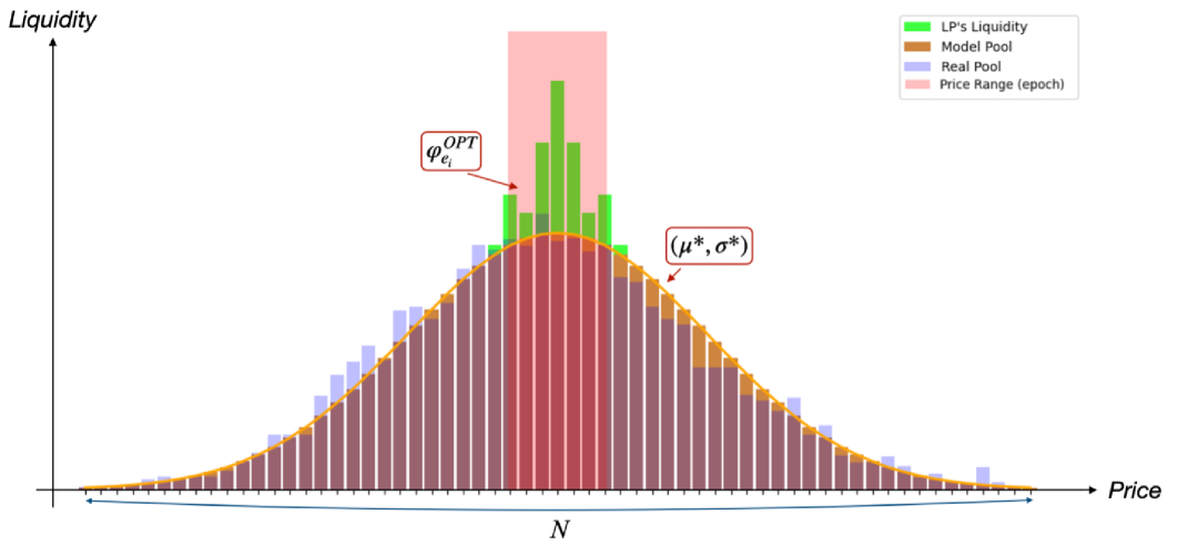
Let the TVL level be allocated across the buckets of the partition during epoch according to the weight vector , , . The capital assigned to the bucket is . Following the Gaussian–curve approach in [6], the weight vector is generated by a normal density with mean and sigma :
| (16) |
where maps the parameters to a discrete Gaussian weight vector over the buckets. These parameters are calibrated so that the model fee matches the historical fee vector defined in the previous subsection. Calibration proceeds by iterating on the Gaussian parameters and over two common grids, , , identical for all epochs. For every candidate pair the following pipeline is executed:
| (17) |
where denotes the model fee (in the chosen numéraire) earned by the pool in epoch when the liquidity distribution follows the Gaussian profile with parameters and . The calibration terminates at the first parameter pair for which the discrepancy between the model fee and the historical benchmark falls within the prescribed tolerance:
| (18) |
Thus, the calibrated pair achieves the closest match between the model fee and the observed pool reward in epoch . Theoretically, the first chosen pair of parameters might not be the only possible one, but this can occur only in two cases:
-
1.
The historical prices within the active ranges of the epoch are nearly uniformly distributed; or
-
2.
The prices are concentrated in the neighborhood of the current reference bucket.
In either situation, selecting the first admissible parameter pair does not affect the resulting shape of the optimal LP strategy.
Stage 2: LP balance equation.
The shares are derived from the liquidity vector and an epoch-specific weight vector , , , where . The -reset strategy imposes sparsity on : positive weights appear only in the buckets centered on the reference index . Hence
| (19) |
Analogous to the pool–side approximation in equation (17), the chain of dependencies that generates LP fees in epoch under the -reset strategy can be summarized schematically as
| (20) |
Here is the value (in the chosen numéraire) of the fee stream paid to the LP for the supply of liquidity under strategy , given the approximated pool profile characterized by . Assuming the approximated profile remains fixed throughout epoch and that in-pool prices track their market counterparts, the end-of-epoch value of the LP’s position is
| (21) |
where and the notation follows (9)–(10). Equation (21) expresses the LP capital after accounting for both impermanent loss and accrued fees. It should be noted that when epochs, the researcher can do so:
-
1.
Reinvest at the start of epoch , thus compounding the fee income.
-
2.
Refrain from reinvesting fees, leaving the working capital exposed to impermanent loss and subject to -reset execution costs, as illustrated in part 5.4 of [6]; or
-
3.
Keep vector constant across epochs, implicitly assuming an unlimited supply of deployable liquidity.
2.4.4 Optimal strategy selection.
For each epoch the search for an optimal LP strategy is performed over a finite family of -symmetric capital allocations. Let be the capital to be deployed and the associated weight vector (cf. (19)); -symmetry requires , , where is the reference bucket of epoch . Let be the finite family of random -strategies, where is the number of candidate strategies examined. The optimal strategy maximizes the modeled fee income defined in (20):
| (22) |
The present study focuses on LP rewards model and does not address the complete liquidity management strategy; this larger problem is left for our next research. Consequently, the buy and hold strategy is not employed as a benchmark in the current study. The set of optimal epoch strategies serves as the target output to train the machine learning model described in the next section.
2.5 Architecture of the Core ML Model
The machine learning (ML) model is used to infer the optimal liquidity allocation strategy from the prevailing market state. Its input features are quantitative descriptors of market conditions at the decision time; the model outputs the weight vector associated with the optimal LP strategy. Training is carried out on historical data that comprise, for each epoch of the modeling period, the optimal strategies obtained by solving the problem (22); the set of features reflects the market conditions at the beginning of the corresponding epoch. A detailed specification of the model architecture, the feature engineering pipeline and the hyperparameter configuration is provided in Section 4.
2.5.1 ML model architecture.
For each epoch , the optimal LP strategy is represented by the weight vector , whose non-zero entries occupy the buckets . Collect these entries in the vector , and exploit the -symmetry for to define the reduced representation . Stacking the epoch vectors yields the target vector
where is the number of epochs. Each epoch is characterized by a feature vector , being the feature dimension, and the feature matrix is
The learning task is to approximate the mapping using a supervised ML algorithm. The dataset is partitioned 80/20 into training and test subsets.:
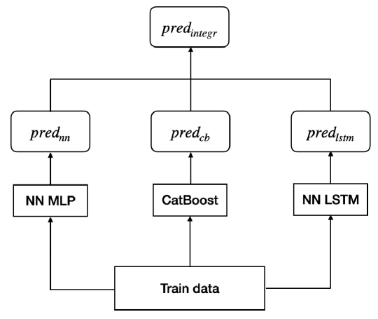
with and . An integrated ensemble model is used, which combines a multilayer perceptron (MLP), gradient-boosted CatBoost decision trees, and a long-short-term memory (LSTM) network. The models are trained on , tested on , and subsequently applied to an out-of-time (OOT) period that simulates real-world deployment . One of the simplest, yet most effective, model fusion techniques is weighted linear prediction averaging:
where and . The weights are chosen to minimize the error on the train date. A schematic of the ensemble is shown in Fig. 2.
Full implementation details - network hyperparameters, feature engineering, and evaluation metrics - are provided in Section 4.
2.6 Reward Modeling Approaches
Four principal approaches can be distinguished when modeling fee accrual in DEX liquidity pools:
-
1.
Pool-level reward modeling: reproducing the aggregate fees earned by the entire pool.
-
2.
Single-LP reward in an isolated theoretical pool: evaluate the fees of a lone liquidity provider in a hypothetical pool that contains only the liquidity of that provider.
-
3.
Single-LP reward as a share of historical pool liquidity: calculate the fees of an LP relative to the actual historical liquidity present in the pool.
-
4.
Single-LP reward in a pool augmented beyond its historical liquidity: computing an LP’s fees after injecting additional model-generated liquidity on top of the historical pool state.
Each approach is analyzed in detail, together with its advantages, limitations, and key modeling assumptions.
2.6.1 Approach 1: pool-level reward modeling.
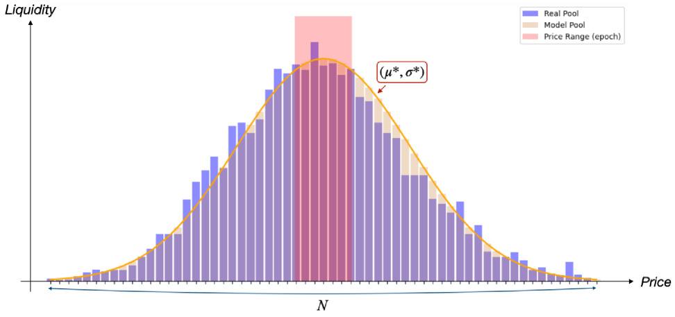
The first approach focuses exclusively on reproducing the historical fee income of the pool. Given a fixed average TVL marked as , different liquidity profiles (concentrated to varying degrees) can generate different fee levels in the same set of active ranges, because the trade volume required to move the price along the prescribed path depends on how liquidity is distributed within the pool.
By selecting the shape parameters of the Gaussian liquidity profile according to equation (18), the modeled pool reward can be brought within a prescribed tolerance of the historical reward realized. This procedure establishes a direct link to the empirical fee level and thus supplies a natural benchmark for the calibration of the synthetic liquidity profile.
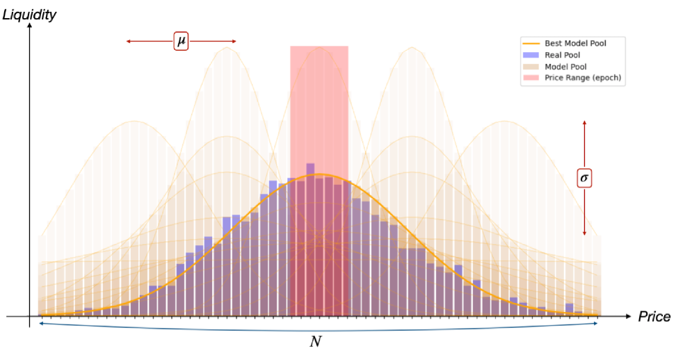
Methodological details.
Following the Section 2.4, the liquidity profile of the pool is approximated within each epoch by sweeping the two Gaussian parameters and as illustrated in Figure 3. The outer boundaries and of the partition are chosen to coincide with the empirical limits of liquidity deployment observed over the historical period, while the number of buckets is selected so that the implied bucket width does not fall below the minimum tick size of the modeled pool. The average TVL level is specified in accordance with Section 2.1.
of the pool’s historical liquidity.
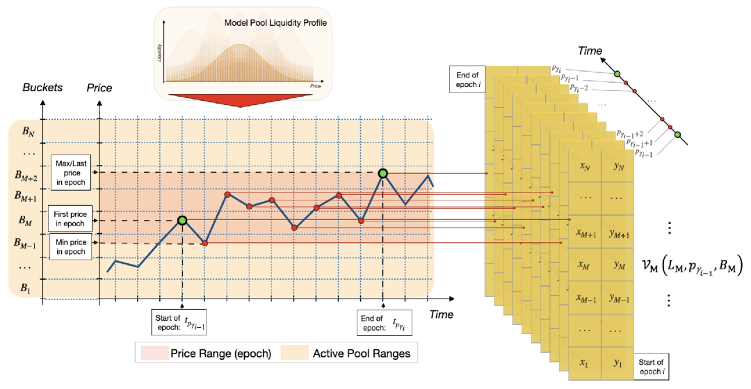
Once the Gaussian parameters have been swept, the liquidity profile for each epoch is fixed by solving Eqs. (7)–(9) over the price path . The peak of the Gaussian curve is located at the mean price of the epoch . Figure 4 illustrates, for a representative choice of , how the reserve state in each bucket evolves as historical prices move. Figure 5 shows an example of the calibrated profile obtained with the pair of parameters for which the model fee matches the historical fee within the researcher’s tolerance.
It should be emphasized that this methodology constitutes the core of [6]; in the present work it is retained as an integral component of the remaining LP reward modeling approaches.
2.6.2 Approach 2: single-LP rewards in an isolated, theoretical pool.
This case, essentially a hypothetical-pool model - considers an individual LP as the only liquidity provider. Unlike Approach 1, no natural fee benchmark exists because the simulation is decoupled from the historical trade volumes of any specific pool. The optimal strategy is therefore the strategy that maximizes the model fee level, without reference to the Gaussian parameters used to approximate historical liquidity.
Although not implemented in the empirical part of the present study, the approach is included here for completeness. Its optimization problem mirrors the Eqs. (18), (22) reads as
| (23) |
where the LP strategy prescribes liquidity allocation, and the pool liquidity vector depends only on the LP’s own capital,
In essence, this is a special, single-provider case of Approach 1; yet it is highly stylized, because only in a theoretical setting would the price path mirror the historical trajectory of a real pool in the presence of an arbitrary liquidity surface supplied by a lone LP.
Methodological details.
Adopting the framework of Section 2.4, the boundaries of the outer bucket and are first set to span the admissible liquidity range in the hypothetical pool. The researcher then selects such that the width of the bucket does not fall below the minimum tick size of the pool. Because the sole liquidity provider is the LP, the TVL pool equals the LP capital .
For each epoch and the fixed price path , random –symmetric strategies are drawn from . The optimal strategy maximizes the income from the LP’s fee and, by construction, coincides with the pool model fee: is therefore concentrated in ranges, mirroring Stage 2 from Section 2.4 but at the pool level rather than for an individual LP. Figure 6 illustrates how the liquidity state in each bucket changes while historical prices evolve under one realization of the strategy.
To conclude, although the isolated pool framework is conceptually valid, its practical relevance is limited; therefore, the foregoing description is sufficient, and the paper now turns to the core approach of this research.
together with the corresponding optimal LP strategy for epoch .
2.6.3 Approach 3: LP rewards as a share of historical pool liquidity.
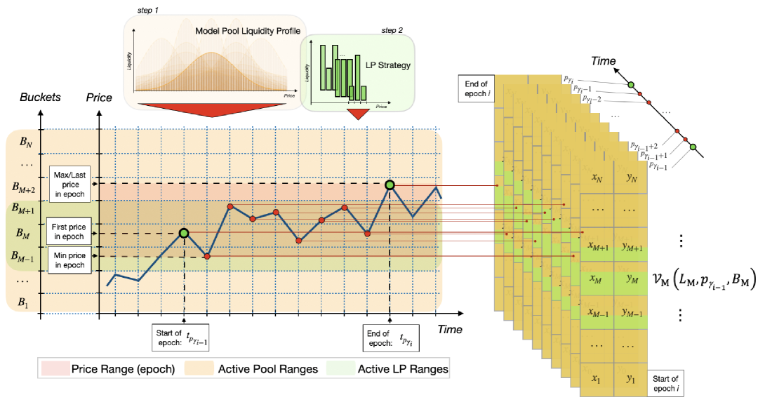
This and the next approaches address the optimization problem in (22). The distinguishing feature of the present approach is its two-stage structure as described in Section 2.4:
-
1.
Stage 1. For each epoch the liquidity profile of the pool is first calibrated by solving (18), resulting in the pair of parameters such that the model fee matches the historical fee . This step exactly replicates Approach 1 and produces the approximate liquidity of the pool .
-
2.
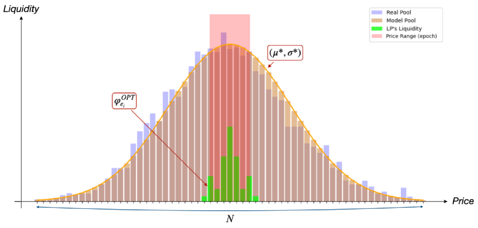
Stage 2. Conditional on , the optimal LP strategy is selected as the maximizer of ; cf. (22).
In this setting, the model LP reward is determined by the share vector that quantifies the proportion of liquidity held by the LP in each active price range of epoch (Fig. 7). A practical implication is that the historical pool reward constitutes an upper bound on the attainable LP reward: the LP cannot earn more than the fee potential embedded in the approximate pool profile specified by .
Methodological details.
As in Approach 1, the partition and the TVL level are fixed first. Given the price path , the liquidity surface of the pool for epoch is calibrated by sweeping the Gaussian parameters and until the model fee matches the historical fee within the preset tolerance.
With the initial LP capital and the same price subset , a random search of the strategy family (for the fixed parameter ) produces the optimal strategy that maximizes the LP reward within the liquidity of the approximated pool, cf.(22). Figure 8 illustrates how the liquidity state in each bucket changes while historical prices evolve, and in the buckets of contains, among other components, the LP-position in the form of dictated by .
Practical caveat.
If the capital allocated under a candidate strategy is sufficiently large, it can happen that in some bucket the liquidity of the LP exceeds the approximate liquidity of the pool . In that case, the model assumes that the LP captures all the historical fees generated in that bucket during epoch , but never more; see Fig. 9(a). This situation is admittedly unrealistic because it assumes that the LP can absorb the entire historical liquidity and collect the full fee stream, an outcome attainable only when represents a non-negligible fraction of the TVL pool - in the extreme, matching it, Fig. 9(b).
Although this case pushes the model away from empirical plausibility, it can be mitigated by (i) choosing in the simulations, or (ii) imposing additional constraints on the shape of the approximating liquidity profile to prevent a single LP from dominating any active bucket.
2.6.4 Approach 4: LP rewards in a pool augmented beyond its historical liquidity.
Like Approach 3, follows a two-stage workflow. First, the historical liquidity surface is recovered by Approach 1, producing the calibrated vector . Next, for a given LP capital the optimal strategy is obtained from (22), maximizing the LP model fee in epoch .
The distinguishing element of the present approach is that LP fees are calculated after local expansion of historical liquidity by the LP’s own liquidity into buckets centered on the reference index . Thus, the fee share is taken relative to the augmented liquidity profile - historical plus the additional capital of the LP - see Fig. 10.
Methodological details.
This approach follows the same two–stage workflow described in Section 2.4, with one modification. After finding the Gaussian parameters so that , the approximated historical liquidity vector is augmented by the LP’s liquidity generated by a candidate strategy . The updated liquidity vector is The optimization pipeline, analogous to (20), becomes
| (24) |
where the share vector is calculated with respect to the increase in liquidity . The strategy is then selected as the maximizer of , subject to the configuration of the augmented pool.
Practical caveat.
Unlike Approach 3, the historical fee level no longer serves as an upper bound for the modeled LP reward. If the injected capital is sufficiently large, the LP can impose an extreme liquidity concentration within the active range, so that the historical share of liquidity held by all the other providers tends to zero. In the limit, the situation reverts to the hypothetical single-LP pool of Approach 2, which seems unrealistic. This pathological result can be avoided by enforcing when simulating the strategy.
Another assumption concerns the nature of the trades that generate the historical price set . If it is posited that every price update was driven exclusively by arbitrage trades executed by informed traders, then Approach 4 remains internally consistent: the additional LP liquidity, however concentrated, does not impede arbitrageurs from supplying the trade volume required to reproduce the historical price path. However, in reality, a non-arbitrage order flow is always present, and its volume is unlikely to scale with the LP super-concentration. Consequently, the real trade volume would fall short of that model volume, dampening the realized price volatility of the pool and activating fewer price ranges than in the original history, which in turn reduces the modeled LP reward. Ideally, therefore, the practitioner should either (i) mark historical swaps as arbitrage or non-arbitrage and retain only the former when simulating with super-concentration, or (ii) estimate the arbitrage share ex ante and adjust the modeled LP reward downward to reflect the liquidity that genuine arbitrage trades can reasonably provide.
3 Related Work
This section includes a number of papers studying liquidity provision in CLMM markets, specific strategies and backtest frameworks, as well as papers on ML applications for CLMM markets.
The concept of liquidity provision in the context of concentrated liquidity has been studied in the literature from several angles. Popular research topics are impermanent loss, trading fees in the DEX market, DEX market overall design, liquidity provision strategies, and many others.
The liquidity provided into a DEX pool both for the CPMM and CLMM cases is an option-like property with the corresponding nonlinear payoff function and effects caused by volatility and elapsed time. The general results behind an abstract liquidity pool have been developed in [7], and [9]. There, one can find all the necessary calculations to deal with token reserves, swaps, fees, and liquidity. Moreover, in [10] the authors provide a methodology to estimate the accumulated fees in a liquidity pool with basic assumptions on the price behavior, but do not explicitly consider the trading volumes.
To understand the properties of a decentralized exchange from the point of view of a trader, consider the paper [11] in which the authors compare the price discovery process in a DEX with the centralized market and study the behavior of informed traders. In the paper [12] the authors work with the bid and ask prices in the context of a liquidity pool and derive the value of a no-trade gap.
Among the important papers which study the impermanent loss one should mention the paper [13] where the authors study the risks of a liquidity provider and the potential returns which may be obtained from such activity. The model allows to dive into the liquidity provision problem from the point of view of a cautious investor and allows to look at the numerical estimations from the real-world data developing solid intuition to deal with such kind of problems.
The next paper to consider is [14] where the authors provide an estimate that half of the liquidity providers lose money in the dataset considered in the paper. This is a reminder that liquidity provision is very complicated in the case of concentrated liquidity, and one must deal with option like payoffs as well as with dynamic reallocation decisions to capture the fees depending on the market conditions.
To understand the concept of impermanent loss even deeper one should dive into the [15] paper which not only provides a concise and instructive result to estimate the impermanent loss but also generalizes the concept allowing to compare the potential loss not only to the buy and hold strategy but also to any benchmark strategy available to the investor with a special case of the rebalancing strategy producing the corresponding loss versus rebalancing metric.
Dealing with impermanent loss is a complicated problem, a general approach is hedging the risk with classic options. The following study [16] applies arbitrage-based methods to produce both a static and a dynamic hedge for the impermanent loss and derive explicit formulae in the case of a Black-Scholes-Merton model and the log-normal stochastic volatility model.
The concepts described above are the important building blocks necessary to construct a liquidity provision strategy for a CLMM market. The strategies studied in the paper are based on the concept of -reset described in [5].
A notable paper studying liquidity provision strategies is [17] where the authors consider a CLMM and consider the accumulated fees, rebalancing costs and the liquidity concentration risk. This is a continuous time model which allows to analyze asymmetric liquidity provision strategies for specific market conditions.
The paper [18] considers the problems arising in the liquidity pools in continuous time. The authors consider a continuous time model for the liquidity dynamics in a CLMM pool. Both finite and infinite horizon settings are considered with an assumption that the liquidity provider should rebalance the strategy when the price goes out of the price range. Following this research it is also important to mention a very promising piece of research considering liquidity provision as an optimal stopping problem [19]. This approach allows to look at the liquidity provision problem from a new point of view and is important to consider for the general idea of a dynamic liquidity provision strategy.
The papers described above focus on modeling and developing theoretical results meanwhile an efficient way to work with liquidity provision strategies is based on numerical analysis and machine learning techniques. Several papers study CLMM liquidity provision from this point of view, for example in the paper [20] the authors apply the deep reinforcement learning approach to maximize the accumulated fees corrected for the loss versus rebalancing risk, and optimize the price interval width, lower and upper bound of the interval. Another paper with a similar strategy and deep reinforcement learning approach is studied in [21], where the authors demonstrate better strategy performance compared to a benchmark on the example of ETH/USDC and ETH/USDT pools.
The reinforcement learning approach is applied not only to liquidity provision strategies but for the AMM design to create a more efficient market decreasing the impermanent loss and slippage, as shown in [22].
Efficient decentralized market design is another important topic to understand the ideas behind optimal liquidity provision. The paper [23] introduces the concept of a general decentralized liquidity pool and allows the liquidity provider to use dynamic bonding curves for more efficient trading. And the paper [24] extends the problem even further considering the trading platform itself as another player competing for the trading fees with the liquidity providers.
In the context of current research, it is important to remember that the liquidity provider is not a single player in the pool, there are many different liquidity providers who compete to earn more fees while controlling for the risk of impermanent loss. In the paper [25] the authors apply a mean-field game approach to analyze the resulting liquidity distribution which appears as the result of many liquidity provision strategies and also consider the case of just-in-time liquidity as an extension of the model. A model specifically focused on just-in-time liquidity is studied in [26].
The research papers discussed above allow to achieve deep understanding of the liquidity provision problem, the only element left out in the context of strategies is backtesting. To understand whether the strategy is of any use for practice one must launch it in a real liquidity pool or consider a robust simulation environment allowing to estimate the amount of fees accumulated by the strategy in the pool. General ideas behind the problem of strategy backtesting for CLMMs have been studied thoroughly in our previous paper, we refer the reader to the paper [6] for deeper analysis.
In this paper, we apply the accumulated knowledge of the concentrated liquidity pools mechanics to extend the backtesting framework research and use it for better liquidity provision activity using machine learning methods for to obtain numerical results for the strategies in specific market conditions within the family of -reset strategies.
4 Modeling on Real Data
In this section, the methodology developed above is applied to real Uniswap V3 data. A uniform-liquidity strategy is used as a benchmark, while the proposed approach is evaluated on data from USDC/ETH pools with several fee levels, in stablecoin pools and in WBTC/ETH. The section ends with (i) a summary of the consolidated performance of all pools, (ii) a comparison with an external backtesting tool, and (iii) a high-level schematic of the application of the ML model for liquidity allocation decisions.
The step-by-step exposition in current section focuses on the USDC/ETH pool with the 0.3%111Contract 0x8ad599c3A0ff1De082011EFDDc58f1908eb6e6D8 fee tier; the accompanying Jupyter notebooks with code, hyper-parameters, and raw data are available on GitHub [27]. General details and modeling approach:
-
•
In-sample period. Swap transactions and trading volumes from 1 April 2023 to 30 June 2024 serve as the training modeling period .
-
•
Out-of-time (OOT) period. Model deployment is emulated on the perod 1–30 September 2024.
-
•
Reward approach. The third approach of Section 2.6.3 was adopted because it links the level of synthetic fees to the historical upper bound, which yields conservative expectations for the OOT analysis.
Historical swap-transaction data were retrieved using GraphQL queries to the Uniswap V3 subgraph.
4.1 Historical Liquidity Approximation and Optimal LP Strategy Search
According to the proposed methodology, the modeling is performed in two stages:
Stage 1: approximating of the historical liquidity profile.
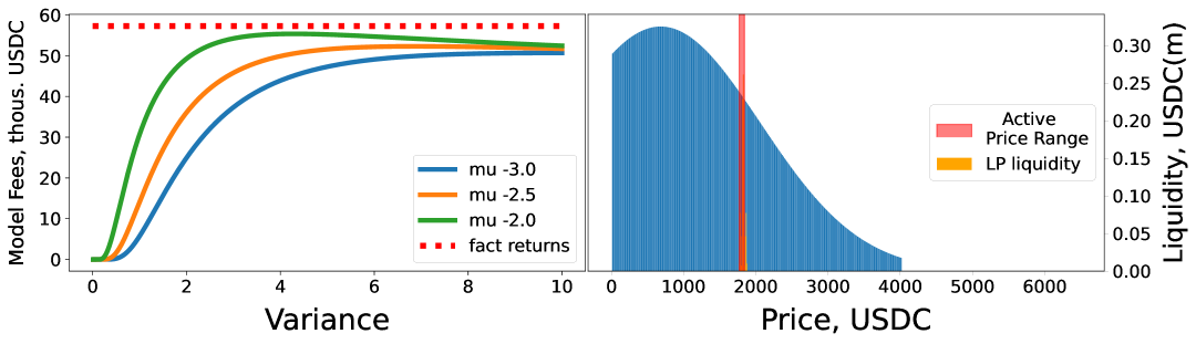
For every epoch the pool’s liquidity shape is approximated by sweeping the Gaussian parameters and until the reward of the modeled pool deviates from the historical value by no more than . The average TVL is fixed at USDC, width of the bucket USDC, lower boundary and . Applying the -reset rule with partitions the in-sample period into epochs. The cumulative historical fee USDC is matched by the modeled fee USDC, that is, an approximation error of about , well inside the tolerance. Figure 11 illustrates the calibration for the first epoch: the optimal parameters and yield USDC versus historical USDC (error ). The right-hand panel of Fig. 11 shows the resulting liquidity profile and the active price range of epoch (in red).
Stage 2: determination of optimal LP strategies.
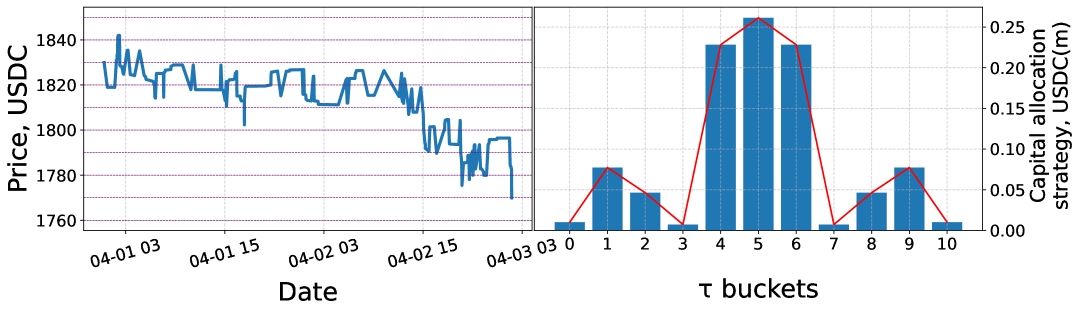
Once the historical liquidity is approximated, the optimal LP strategy is found by solving the problem (22). At the start of each epoch the LP deploys the same initial capital million USDC; inter-epoch capital dynamics are ignored at the training stage to isolate each epoch.
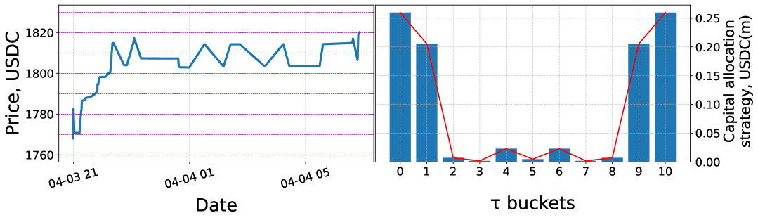
For epoch the optimizer produces the vector shown in Fig. 12 (right), which aligns with the price path in the left panel and delivers a modeled LP fee of USDC.
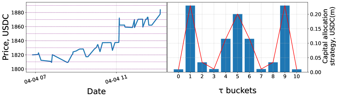
Additional examples are provided in Fig. 13 (epoch ) and Fig. 14 (epoch ), where optimal allocations shift towards the buckets that capture most of the observed price movement. This provides an intuitive and visually compelling demonstration of the concept of optimal strategy. Collecting optimal allocations for all epochs yields the target vector used to train the ML model, as defined in Section 2.5.
4.2 ML Model Training and Features Engineering
Within the present study the architectural nuances of the machine learning models do not constitute the main focus of the research. Each model is deployed in a baseline configuration with no systematic hyper-parameter tuning. The emphasis is on demonstrating the capabilities of the proposed methodology and the accompanying backtesting framework: in particular, the ability (i) to determine optimal LP strategies ex post, (ii) to record the market-state feature values at the moments of optimal allocations, and (iii) to use the resulting patterns for future liquidity-allocation decisions.
Feature engineering is also intentionally minimal. All inputs are derived from only two raw numerical indicators, from which a compact set of features is generated to capture latent patterns in market dynamics. The approach is generic and can be adapted to any collection of numeric variables. Subsequent sections confirm that even such sparse feature sets and simple model configurations are sufficient for the goals of this work.
4.2.1 ML Model Architecture.
The predictions of the integral model are produced by a weighted ensemble of three base learners: an MLP neural network, CatBoost, and an LSTM network. The remainder of this subsection details the architectures implemented in the experiments, including structural choices, theoretical rationale, hyperparameter settings, regularization techniques, and evaluation metrics.
MLP neural network.
Fully connected neural networks (multilayer perceptrons, or MLPs) are universal function approximations and are widely used for regression and classification tasks. The core idea is to propagate the input feature space through a sequence of hidden layers equipped with non-linear activation functions, thereby capturing complex relationships between inputs and targets. Key settings:
-
•
Loss function: Mean Squared Error (MSE).
-
•
Optimizer: Adam.
-
•
Training schedule: 100 epochs with early stopping.
-
•
Regularization: EarlyStopping callback.
-
•
Validation: 5-fold cross-validation with the best model retained.
Network architecture:
-
•
Input layer - dimensionality equals the number of features in .
-
•
Hidden layers
-
–
Dense(128, activation=relu)
-
–
Dense(64, activation=relu)
-
–
Dense(32, activation=relu)
-
–
Dense(16, activation=relu)
-
–
-
•
Output layer: Dense
CatBoost (gradient boosting on decision trees).
CatBoost is a gradient boost implementation optimized for categorical features and known for its robustness to overfitting [28]. It is used here as a high-accuracy regression learner on tabular data. Key settings:
-
•
Loss function: MultiRMSE.
-
•
Tree depth: 6.
-
•
Number of iterations: 1000.
-
•
Boosting type: Plain.
-
•
Early stopping: enabled.
-
•
Validation: 5-fold cross-validation with model selection.
LSTM (Long Short-Term Memory network).
LSTM networks are a class of recurrent neural networks (RNNs) designed to handle sequential data and long-term dependencies. Although each training instance in this work represents an aggregated snapshot of features at a single point in time, an LSTM is included as an alternative to the MLP, capitalizing on its ability to model internal patterns within the aggregated feature structure. Key settings:
-
•
Loss function: Mean Squared Error (MSE).
-
•
Optimizer: Adam.
-
•
Training schedule: 100 epochs with early stopping.
-
•
Regularization: 20 % dropout after the LSTM layer.
-
•
Validation: 5-fold cross-validation.
Network architecture:
-
•
Input - vector of one-dimensional temporal features .
-
•
Hidden layer: LSTM(128, activation=relu).
-
•
Dropout layer — rate 0.2.
-
•
Output layer: Dense
Although every training instance in the data set is an aggregated snapshot of market features taken at a single time stamp, an LSTM network is nonetheless included as an architectural alternative to the MLP. The objective is not to extract temporal autocorrelations across successive observations - by construction, such correlations are absent - but rather to exploit the LSTM gating mechanism as a powerful non-linear/combinatorial feature extractor. Thanks to its cell state and input/forget gates, an LSTM can learn structured interactions and hierarchical patterns that arise inside the high-dimensional vector of engineered features, even when those features are computed from historical time series and then collapsed into a single observation.
A further consideration is that LP reallocation events (i.e., the epoch boundaries) may be widely spaced and occur at irregular intervals, making classical sequence-modeling assumptions difficult to satisfy. By embedding an LSTM block in the ensemble, the model gains a neural component whose internal dynamics differ markedly from those of an MLP; this architectural diversity is expected to enhance the ensemble’s ability to generalize outside of the sample.
Integral model (ensemble by weighted averaging).
The final prediction is obtained by a weighted sum of the three base models. The optimal weight vector is found by minimizing the mean square error with regularization () under the constraints and .
Optimization is carried out with the Sequential Least Squares Programming (SLSQP) algorithm, an efficient method for constrained nonlinear optimization. SLSQP is particularly well suited here because (i) it directly handles the simplex constraints on the weights, (ii) the ensemble layer involves only three parameters, so the computational burden per iteration is negligible, and (iii) the problem is convex, ensuring a globally consistent solution.
4.3 Feature Engineering
Centralized exchange (CEX) data serve as the information set to characterize the market state in each allocation decision. Historical market data are sourced through the live_trading_indicators222https://pypi.org/project/live-trading-indicators/ library, which offers unified access to multiple cryptocurrency exchanges. For the USDC/ETH pool, the study employs one-minute OHLCV bars for the USDC/USDT and BTC/USDT pairs on Binance, covering 1 March 2023 to 30 September 2024; the inclusion of BTC captures potential cross-asset comovement with ETH. For other pools, the same procedure is followed: features are generated for both the target pair and the BTC.
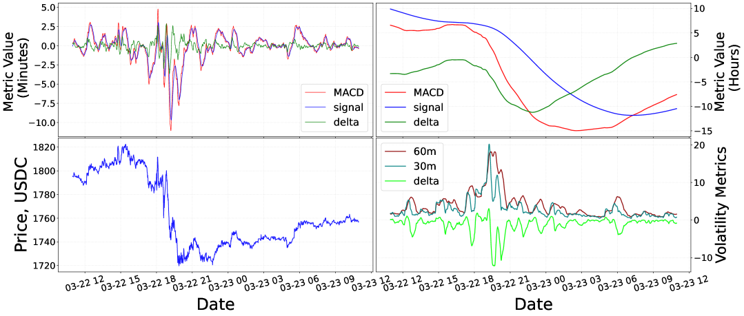
Each bar provides the closing price and traded volume; the timestamp is used as the index. For every epoch, the feature vector is generated at the beginning of the epoch (index in Section 2.2) by selecting the nearest CEX timestamp. The other indicators are the exponential moving average (EMA) and the moving average convergence divergence (MACD) — fundamental tools of technical analysis that highlight trend and momentum behavior.
The market features for the ML model are derived from two pairs of cryptocurrency: USDC/ETH and BTC/USDT according to the following algorithm:
-
1.
Data retrieval. One-minute OHLCV bars are downloaded from Binance for the symbols ethusdt and btcusdt. The closing price (feature 1) and trade volume (feature 2) are retained.
-
2.
Volume clearing. Zero volumes, if any, are replaced with a small constant () to avoid numerical errors in subsequent calculations.
-
3.
Sliding-window indicators (minute scale).
-
(a)
Two exponential moving averages (EMAs) with periods 12 min and 26 min are computed (features 3 and 4).
-
(b)
The MACD line is defined as the difference between the two EMAs (feature 5); the signal line (feature 6) is the 9-period EMA of the MACD, and their difference (feature 7) completes the trio.
-
(a)
-
4.
Sliding-window indicators (hour scale). Steps in 3 are repeated in the hourly aggregation (12 h and 26 h windows), producing features 8-12.
-
5.
Volume-volatility measures. Rolling standard deviations of the trade volume are calculated over 30- and 60-minute windows (features 13 and 14); their difference provides feature 15, quantifying the change in volume turbulence.
For each pair, the above procedure outputs 15 features (Fig. 15); the same calculations for the second pair and the pairwise ratios between the two sets enlarge the feature vector to 45 dimensions. Thus, at the start of each epoch the market state is represented by and the complete design matrix is (Section 2.5).
Look-back horizon. At every liquidity reallocation (or initial provisioning), the feature algorithm consumes a one week history ( minutes) preceding the decision time. This window can be shortened or extended for specific indicators if required, but a uniform horizon is adopted here for the sake of clarity.
Remarks on feature selection. Standard feature selection techniques could be applied to reduce multicollinearity; however, the complete set is deliberately retained to emphasize the generality of the methodology rather than to maximize predictive accuracy through aggressive pruning. In addition, all three base learners are trained in the same feature matrix, which simplifies comparison and integration of the ensemble, albeit at the cost of avoiding model-specific feature customization - an acceptable trade-off given that architecture optimization is not the main objective of the study.
4.4 Application of ML Models to the OOT Sample
The out–of–time (OOT) period comprises all swap transactions and volumes recorded in the pools between 1 and 30 September 2024. With the exception of the locked total value , all modeling hyper-parameters are retained from the training part.
In live operation, the model requires only the current feature vector to output an allocation decision. However, for retrospective fee backtesting, the full workflow of Section 4 must be repeated, still relying on the third reward modeling approach, but without enumerating random LP strategies. The optimal strategy for epoch is supplied directly by the ML model and is denoted .
The bucket grid is fixed (its boundaries may differ from the training grid, but the tick size must be unchanged), and the historical liquidity in the active ranges now approximating with an updated average TVL of USDC. Apart from this change, the algorithm mirrors the training procedure, subject to the additional considerations described next.
4.4.1 Specific Assumptions for OOT.
A more refined liquidity approximation scheme is employed for the OOT period in order to produce a tighter fit to the observed swap flow.
for the cases (a) and (b).
In the advanced approach, the approximate liquidity profile is not kept fixed over the whole epoch . Instead, a sliding window of length trades is fitted successively times within the epoch. The historical pool fee is therefore decomposed as so that is represented by sub-epochs, each endowed with its own calibrated parameters for . The number of sub-epochs is
| (25) |
where and can be represented as , where is the remainder of trades that is insufficient to form another full window and is therefore appended to the last sub-epoch. This granular calibration reproduces the historical fee flow almost down to the individual-swap level, delivering a more faithful representation of pool dynamics in the OOT period (Fig. 16).
The window length is user-defined and controls the degree of flexibility of the model liquidity: LP capital as vector is still fixed at the start of , but the provider’s share evolves with each sub-epoch, producing distinct ratio vectors instead of a single . Flexibility in epoch is quantified by
| (26) |
so that for (maximal dynamics, one approximate per price change) and for when (a single static approximate, as in the training part).
To prevent unrealistically large LP shares in narrow ranges (cf. Fig. 9), a conservative rule is imposed: whenever the found approximated parameter , the LP fee contribution for that sub-epoch is set to zero. Denoting this liquidity-rule form as LRF, curtails excessive fee projections that could arise from an over-concentrated placement.
4.4.2 Results on the OOT period.
Using the same procedure as in Section 4, the OOT price set , the bucket grid and the -reset rule partition the period (1–30 September 2024) into epochs with . Applying the algorithm of Section 2.6.3 together with the flexibility of the model liquidity () and the LRF constraint, problem (18) is solved for every sub-epoch.
The aggregated historical fee for the OOT period is USDC; the model reproduces this value with USDC, which corresponds to an approximation error of approximately .
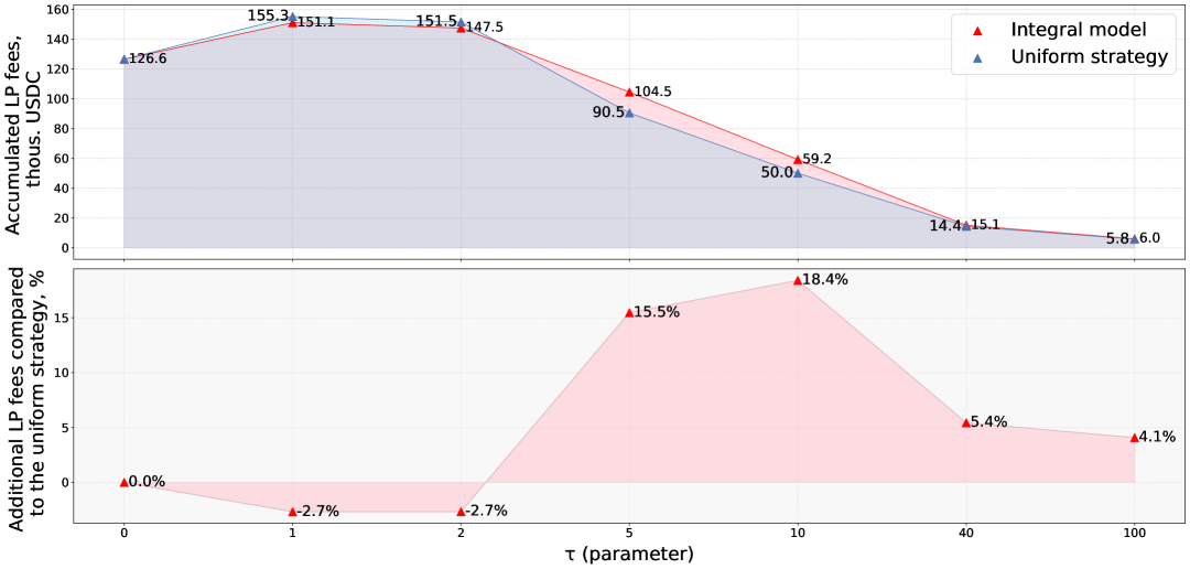
The pool is then analyzed with respect to the impact of the allocation parameter on modeled LP rewards. Figure 17 and Table 1 compare the results of the optimal ML model strategy with a uniform-liquidity baseline. The relationship between values and the corresponding metrics is demonstrated, including epochs, average time, number of elements, fee values, and percentages of ML model efficiency. The case represents a single-bucket placement in the reference bucket .
It should be emphasized that the initial capital m USDC; however, unlike in the training part, the working capital evolves over time for . Now, two additional components are taken into account:
-
•
Gas expenditure. Deploying liquidity in a single range is charged gas units, whereas burning liquidity costs gas units. If the amount of LP liquidity in a given bucket remains unchanged after reallocation, the associated gas cost is ignored, in line with the convention of [6]. A constant gas price of is assumed.
-
•
Impermanent loss and downside (market) risk. Beyond accounting for impermanent loss during epoch transitions, should the pool price fall below the lower boundary of the outermost LP-liquid bucket in epoch , the mark-to-market losses are fixed and decrease the LP’s capital.
Throughout the OOT backtesting, all fees are not reinvested between epochs; this separation isolates the modeled reward stream from the evolving principal .
For the USDC/ETH pool with 0.3% fee level, the experimental framework reveals a clear relationship between liquidity concentration (depending on ) and expected reward, with a seemingly counterintuitive exception for and (Fig. 17). The left-hand skew arises from two opposing factors:
-
1.
Heightened negative impact of impermanent loss and more frequent realization of market risk when the liquidity is so concentrated.
-
2.
The upper bound imposed by the historical fee volume in each active range (Fig. 9). In live trading a tighter concentration could in principle yield higher fees, but in backtesting the payoff is capped by historical swap volumes.
(first pool USDC/ETH 0.3%)
| Number of Epochs | Avg. (hour) | Avg. (numb.) | LP Fees, thous. USDC | ML eff., % | ||
| ML model | uniform | |||||
| 0 | 127.6 | 127.6 | 0.0 | |||
| 1 | 151.1 | 155.3 | -2.7 | |||
| 2 | 147.5 | 151.5 | -2.7 | |||
| 5 | 104.5 | 90.5 | +15.5 | |||
| 10 | 59.2 | 50.0 | +18.4 | |||
| 40 | 15.1 | 14.4 | +5.4 | |||
| 100 | 6.01 | 5.8 | +4.1 | |||
Together, these effects explain the drop in modeled rewards for the narrowest allocations despite the intuitive appeal of a tighter concentration. Analyzing the experimental results, we derive the following key conclusions:
-
1.
Concentration versus profitability. A more concentrated liquidity placement generally yields higher fees, yet a clear profitability frontier exists: beyond a certain point negative drivers—impermanent loss (IL), downside price moves, and gas expenditure—can erode the initial capital so severely that the earned fees fail to offset the losses (Appendix A).
-
2.
Reward ceiling under the third modeling approach. When modeling inside the historical-liquidity envelope the attainable fee level is capped by the historical pool rewards. With a large model capital it might appear always beneficial to spread liquidity across a greater number of ranges (i.e. larger ); however, this impression is misleading. A high capital level merely causes the LP to occupy 100 % of several buckets while suffering less from negative drivers—a modeling artifact. The solution is straightforward: select . The present study intentionally chooses a high to highlight this issue.
-
3.
When is an ML strategy worthwhile?
-
(a)
Increasing (with fixed bucket width ) lowers modeled fees for both the ML and the uniform strategies, bringing their results closer together (=40 or 100). Furthermore, a broader allocation demands that the ML model cover a larger volatility band over a longer horizon, forcing the optimal strategy towards a uniform placement.
-
(b)
Conversely, a very narrow placement ( or for the present pool) can under-perform the uniform benchmark; the latter’s universality wins out on short prediction horizons. The case is identical for both approaches.
-
(c)
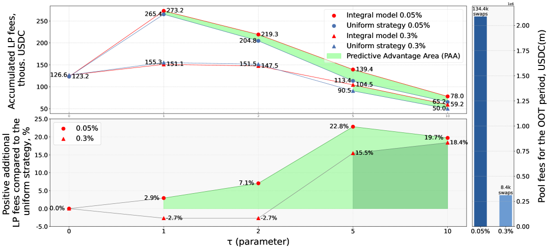
We formalize the concept of predictive-advantage area (PAA) can be identified in which the ML ensemble clearly outperforms the uniform strategy; for the USDC/ETH 0.3 % pool this occurs at and , where the absolute fee difference is maximal.
-
(a)
-
4.
Impact of pool liquidity. Figure 18 contrasts the current pool (USDC/ETH, 0.3 %) with a second pool (USDC/ETH 0.05%333Contract 0x88e6A0c2dDD26FEEb64F039a2c41296FcB3f5640) for . The second pool exhibits an order-of-magnitude larger trade count (134 k swaps vs 8.4 k) and a higher fee volume (2.1m USDC vs 0.3m USDC) over the same OOT period. The price dynamics for the selected period in both pools are presented in Appendix B. Despite the different fee tiers, the qualitative patterns are similar. Owing to the higher turnover, the identical ML architecture has greater scope to surpass the uniform baseline in the more liquid pool; its PAA even extends to . This also can be explained by the fact that higher TVL in more liquid pools reduces the price impact of non-arbitrage trades (non-market factor), thereby enhancing the predictive power of market-feature based ML models in such pools.
4.4.3 Results Across All Pools in the Study.
The proposed methodology and modeling framework were applied to a set of Uniswap V3 pools, including stable-coin pairs, WBTC/ETH and USDC/ETH with different fee tiers. For every pool the initial LP capital was fixed at over the same out-of-time period (1 to 30 September 2024) with the same specific assumptions. The summary statistics are reported in Table 2.
The results demonstrate the versatility of the approach across diverse trading pairs and liquidity profiles. In all cases, the working capital dynamics was tracked without reinvesting the accrued fees between epochs, and the average approximation error for historical pool volumes did not exceed 2%. Stable PAA area emerges at and , where the ML model strategy outperforms the uniform baseline — a steady observation that holds across all examined pools and highlights promising directions for future research on optimal liquidity management in decentralized markets.
4.5 Comparison with an Alternative Tool
To assess general validity, the proposed methodology was compared with Fractal - a modular backtesting library for DeFi strategies released by Logarithm Labs [29]. The key difference between the two tool chains is that Fractal directly ingests historical per-range liquidity, whereas the present framework requires only trade prices and volumes, recovering the liquidity surface via the approximation approach of Section 2.6.
Fractal employs a forward-simulation approach to estimate the LP rewards based on historical Uniswap V3 pool activity from The Graph. The framework iteratively ingests historical data (observations in terms of Fractal): including swap volumes, tick prices, and liquidity snapshots, and then updates the internal state of Uniswap V3 entity, producing backtested performance metrics over time.
The core of fee modeling is aligned with the methodology outlined in the Uniswap V3 whitepaper [2]. To model liquidity placement, the deposit amount is decomposed into token and token allocations, and the strategy’s liquidity contribution is calculated using the canonical Uniswap V3 liquidity formulae. The potential fees earned from the strategy are calculated accounting for the added LP liquidity. This value is then integrated into the Uniswap V3 fee model to estimate the fee income attributable to the LP’s position for a given fee tier and price range. By iterating this process over the full historical time series, Fractal produces backtested strategy results that reflect dynamic fee accruals under realistic market conditions.
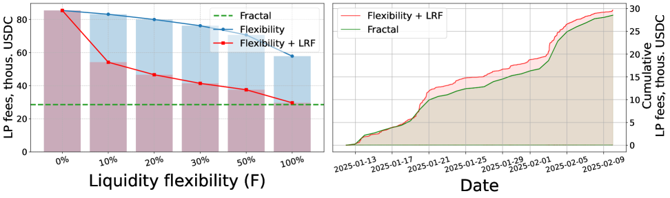
The USDC/ETH 0.3 pool examined earlier was re-evaluated on the period 12 January to 10 February 2025 under identical conditions: and a single epoch (), with one uniform bucket spanning the full price range. Figure 19 contrasts the backtested fee income obtained from the two instruments. The left panel shows the sensitivity of the modeled LP fees to the liquidity–flexibility parameter and LRF constraint; the right panel shows the cumulative fees trajectories over time. With maximum flexibility () the two approaches differ by less than 4% (28 562.3 USDC vs 29 674.2 USDC).
Close agreement with a tool that relies on actual historical liquidity provides additional evidence for the validity of the approximation-based methodology developed in this study.
| Metric | Trading Pools | ||||
| USDC/ETH 0.3% | USDC/ETH 0.05% | WBTC/ETH 0.3% 444Contract 0xCBCdF9626bC03E24f779434178A73a0B4bad62eD | USDC/USDT 0.01% 555Contract 0x3416cF6C708Da44DB2624D63ea0AAef7113527C6 | ||
| Avg. TVL, $M | |||||
| Swap Count, k | |||||
| Range Size | 10 USDC | 10 USDC | 1.23e-4 WBTC | 1.57e-4 USDC | |
| Trading Vol. | USD M | ||||
| Actual | |||||
| Model | |||||
| error | % | % | % | % | |
| Pool Fees | thousand USD | ||||
| Actual | |||||
| Model | |||||
| LP Fees* | |||||
| 147.5 | 219.3 | 132.8 | 3.7 | ||
| 104.5 | 139.4 | 79.5 | 1.9 | ||
| 59.2 | 78.0 | 42.1 | 1.1 | ||
| LP Costs | |||||
| Epochs | |||||
*For LP Fees, first value shows results of uniform strategy, second shows ML model with % additional LP fees compared to the uniform strategy. WBTC-denominated pools show values in USD, converted at the last market price in the OOT period.
4.6 Overall Architecture of the Decision-Making System
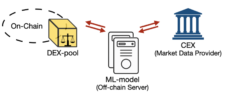
In general terms, Figure 20 outlines how the proposed ML model is deployed within a DEX pool and consists of the following components:
-
1.
DEX pool (on-chain). Holds the liquidity position and the current LP strategy. Whenever the pool price exits the LP-liquid buckets and triggers the -reset rule, an event is emitted to an off-chain server.
-
2.
ML engine (off-chain). Upon receiving the on-chain event, the server queries an external market data source (eg, a CEX) to build the feature vector for the current decision point.
-
3.
Strategy update. The ML model infers the optimal LP allocation and submits the corresponding transaction to the DEX, thereby rebalancing the liquidity ranges.
From a technical standpoint, the interaction between the components can be organized as follows:
-
•
Communication between the DEX pool and the off-chain server can rely on standard Web3 / JSON-RPC interfaces (e.g. an Ethereum node666https://www.alchemy.com/overviews/rpc-node).
-
•
Market data is retrieved from CEX through REST or WebSocket endpoints (OHLCV streams, order-book snapshots, etc.).
-
•
Liquidity reallocation can be executed through a dedicated smart contract wrapper or by directly interacting with the pool position manager contract.
The external data feed does not need to be a centralized exchange; decentralized oracles or DEX aggregators can serve the same purpose while reducing dependence on a single data provider.
5 Conclusions
The advent of concentrated-liquidity AMMs has transformed liquidity provision from a passive activity into an active portfolio management problem: sustainable returns now hinge on consciously selecting price ranges and reallocating capital in a timely manner. Against this backdrop, the task of optimal liquidity provision (LP) is gaining both practical relevance and academic interest.
This study develops, implements, and validates a general-purpose framework for optimal placement of LP in decentralized exchanges with concentrated liquidity. A key distinguishing feature is a custom backtesting approach that reconstructs historical liquidity solely from executed swaps, approximating the per-range liquidity profile to a preset tolerance and thereby eliminating the need for large on-chain state archives. The resulting workflow is light-weight, easy to deploy, and readily scalable. Beyond strategy design and evaluation, the same tool-set can be used to explore alternative AMM architectures.
The empirical focus lies on fee optimization: historical -reset strategies are derived offline, market-condition feature vectors are constructed at each allocation event, and several ML modules are trained and stacked into an integral ensemble. Out-of-time (OOT) experiments on multiple Uniswap V3 pools demonstrate that the ML-driven strategy consistently outperforms a uniform benchmark and that the framework seamlessly transfers between different fee tiers and asset pairs, highlighting its generality and its potential for advancing liquidity management research in the DeFi ecosystem.
External validation against Fractal, an alternative backtesting suite that relies on historical per-range liquidity, shows excellent agreement: the fee estimates differ by less than 4% under identical settings—further supporting the soundness of the proposed methodology.
The broader question of optimizing the live LP position, including hedging and hybrid liquidity placement schemes, has been left for future work. The present framework provides the technical foundation for this endeavor. An open source Python implementation, GPU-accelerated for high-throughput simulations, is available and is intended to foster community adoption and the development of ML-based tooling for DEX optimization.
References
- [1] Buterin, V. A next-generation smart contract and decentralized application platform. White paper, 2014.
- [2] Adams, H., Zinsmeister, N., Salem, M., Keefer, R., and Robinson, D. Uniswap V2 Core, 2020. https://uniswap.org/whitepaper-v2.pdf
- [3] Angeris, G., and Chitra, T. Improved Price Oracles: Constant Function Market Makers. In Proceedings of the 2nd ACM Conference on Advances in Financial Technologies (pp. 80-91), 2020.
- [4] Adams, H., Zinsmeister, N., Salem, M., Keefer, R., and Robinson, D. Uniswap v3 Core, 2021. Tech. Rep. https://uniswap.org/whitepaper-v3.pdf
- [5] Fan, Z., Marmolejo-Cossio, F., Moroz, D. J., Neuder, M., Rao, R., and Parkes, D. C. Strategic liquidity provision in uniswap v3, arXiv preprint arXiv:2106.12033, 2021.
- [6] Urusov, A., Berezovskiy, R., and Yanovich, Y. Backtesting Framework for Concentrated Liquidity Market Makers on Uniswap V3 Decentralized Exchange. Blockchain: Research and Applications, 100256, ISSN 2096-7209, 2025.
- [7] Elsts, A. Liquidity Math in Uniswap v3. Available at SSRN 4575232, 2021.
- [8] Fan, Z., Marmolejo-Cossío, F. J., Altschuler, B., Sun, H., Wang, X., and Parkes, D. Differential Liquidity Provision in Uniswap v3 and Implications for Contract Design. In Proceedings of the Third ACM International Conference on AI in Finance (pp. 9-17), 2022.
- [9] Richardson, M. B., and Loesch, S. DeFi’s Concentrated Liquidity From Scratch. arXiv preprint arXiv:2407.02496, 2024.
- [10] Echenim, M., Gobet, E., and Maurice, A. C. Thorough mathematical modelling and analysis of Uniswap v3. hal-04214315v2, 2023.
- [11] Capponi, A., Jia, R., and Yu, S. Price discovery on decentralized exchanges. Available at SSRN 4236993, 2024.
- [12] Milionis, J., Moallemi, C. C., and Roughgarden, T. A myersonian framework for optimal liquidity provision in automated market makers. arXiv preprint arXiv:2303.00208, 2023.
- [13] Heimbach, L., Schertenleib, E., and Wattenhofer, R. Risks and returns of uniswap v3 liquidity providers. In Proceedings of the 4th ACM Conference on Advances in Financial Technologies (pp. 89-101), 2022, September.
- [14] Loesch, S., Hindman, N., Richardson, M. B., and Welch, N. Impermanent loss in uniswap v3. arXiv preprint arXiv:2111.09192, 2021.
- [15] Milionis, J., Moallemi, C. C., Roughgarden, T., and Zhang, A. L. Automated market making and loss-versus-rebalancing. arXiv preprint arXiv:2208.06046, 2022.
- [16] Lipton, A., Lucic, V., and Sepp, A. Unified approach for hedging impermanent loss of liquidity provision. arXiv preprint arXiv:2407.05146, 2024.
- [17] Cartea, Á., Drissi, F., and Monga, M. Predictable losses of liquidity provision in constant function markets and concentrated liquidity markets. Applied Mathematical Finance, 30(2), 69-93, 2023.
- [18] Tung, S. N., and Wang, T. H. A mathematical framework for modelling CLMM dynamics in continuous time. arXiv preprint arXiv:2412.18580, 2024.
- [19] Hou, L., Yu, H., and Xu, G. Risk-Neutral Pricing Model of Uniswap Liquidity Providing Position: A Stopping Time Approach. arXiv preprint arXiv:2411.12375, 2024.
- [20] Xu, H., and Brini, A. Improving DeFi Accessibility through Efficient Liquidity Provisioning with Deep Reinforcement Learning. arXiv preprint arXiv:2501.07508, 2025.
- [21] Zhang, H., Chen, X., and Yang, L. F. Adaptive liquidity provision in uniswap v3 with deep reinforcement learning. arXiv preprint arXiv:2309.10129, 2023.
- [22] Lim, T. Predictive crypto-asset automated market maker architecture for decentralized finance using deep reinforcement learning. Financial Innovation, 10(1), 144, 2024.
- [23] Cartea, Á., Drissi, F., Sánchez-Betancourt, L., Siska, D., and Szpruch, L. Strategic bonding curves in automated market makers. Available at SSRN 5018420, 2024.
- [24] Takehara, K., Hara, C., Yuasa, T., and Adachi, T. Strategic Interactions in Setting Up Decentralized Exchanges: Conflict of Interest between Liquidity Providers and Platformers. Available at SSRN 4973251, 2024.
- [25] Bayraktar, E., Cohen, A., and Nellis, A. DEX Specs: A Mean Field Approach to DeFi Currency Exchanges. arXiv preprint arXiv:2404.09090, 2024.
- [26] Capponi, A., Jia, R., and Zhu, B. The paradox of just-in-time liquidity in decentralized exchanges: More providers can sometimes mean less liquidity. arXiv preprint arXiv:2311.18164, 2023.
- [27] A. Urusov. Uniswap v3 LP dynamic strategies: source code, data and scripts.
- [28] CatBoost - open-source gradient boosting library https://catboost.ai/
- [29] Research library Fractal https://github.com/Logarithm-Labs/fractal-defi
Appendix Appendix A The state of total liquidity positions versus accumulated fees during the out-of-time (OOT) simulation period
![[Uncaptioned image]](/html/2505.15338/assets/x21.png)
Appendix Appendix B Comparative price analysis between the USDC/ETH 0.05 % and 0.3 % pools during the OOT period
![[Uncaptioned image]](/html/2505.15338/assets/Ap_2.png)
| Symbol | Description |
|---|---|
| Fee tier of the DEX pool (in contract terms) | |
| Set of historical pool prices over the modeling period | |
| Set of historical trade volumes aligned with | |
| Average TVL of the pool during the modeling period | |
| Set of partition of the price axis into buckets | |
| Lower/upper bounds of the -th bucket | |
| Constant width of each bucket in | |
| Liquidity provider’s capital (in the numéraire) | |
| Liquidity provided by the LP | |
| Reference bucket | |
| General parameter of the -reset strategy | |
| Set of LP-liquid buckets | |
| Number of epochs in the modeling period | |
| Index of the last price at -th epoch | |
| Ordered list of epochs | |
| Vector of epoch durations | |
| Vector of epoch lengths (in number of trades) | |
| LP capital allocated to bucket | |
| Real reserves of tokens A and B in bucket | |
| Liquidity allocated to bucket | |
| Current pool price | |
| Liquidity–state function returning for given | |
| Vector of across buckets during epoch | |
| Liquidity vector corresponding to | |
| Increment of real reserves in bucket at price change | |
| Vector of token-wise pool fees in epoch | |
| Vector of token prices expressed in the chosen numéraire | |
| Value of in the numéraire | |
| Aggregate pool fees over modeling period | |
| LP capital at the start of epoch | |
| Bucket-wise vector of | |
| Vector of LP share in total pool liquidity per bucket | |
| Vector of token-wise LP fees for epoch | |
| Value of in the numéraire | |
| Aggregate LP fees over the modeling period | |
| Vector of historical trade volumes per epoch | |
| Vector of historical pool fees per epoch | |
| Weight vector of buckets (entire pool) in epoch | |
| Gaussian mapping that produces | |
| Model fees of pool for epoch | |
| Approximated parameters under which | |
| LP weight vector over buckets in epoch | |
| LP fees under strategy in epoch | |
| LP capital at the end of epoch | |
| Family of random -reset strategies | |
| Optimal LP strategy in epoch | |
| size vector of non-zero elements of | |
| size vector of symmetry-reduced | |
| Vector of optimal strategies over modeling period | |
| Feature vector describing market state at start of epoch | |
| Feature matrix for the ML model | |
| ML-predicted optimal strategy for epoch | |
| Number of sub-epochs in epoch | |
| Liquidity flexibility metric of epoch | |
| LRF | Liquidity-rule form constraint |
| PAA | Predictive-advantage area |