A Note on Spinning Billiards and Chaos

Abstract

We investigate the impact of internal degrees of freedom—specifically spin—on the classical dynamics of billiard systems. While traditional studies model billiards as point particles undergoing specular reflection, we extend the paradigm by incorporating finite-size effects and angular momentum, introducing a dimensionless spin parameter $\alpha$ that characterizes the moment of inertia. Using numerical simulations across circular, rectangular, stadium, and Sinai geometries, we analyze the resulting trajectories and quantify chaos via the leading Lyapunov exponent. Strikingly, we find that spin regularizes the dynamics even in geometries that are classically chaotic: for a wide range of $\alpha$, the Lyapunov exponent vanishes at late times in the stadium and Sinai tables, signaling suppression of chaos. This effect is corroborated by phase space analysis showing non-exponential divergence of nearby trajectories. Our results suggest that internal structure can qualitatively alter the dynamical landscape of a system, potentially serving as a mechanism for chaos suppression in broader contexts.

I Introduction and Motivation

It is remarkable how much you can learn from rolling a ball on a table with a fixed shape boundary! Indeed, despite their seemingly simple dynamics, such classical billiard models play a crucial role in applied mathematics and physics. Classical billiard models are quintessential systems for studying chaotic behavior and nonlinear dynamics. The motion of a particle in a billiard table, especially with irregular or complex boundaries, can exhibit chaotic trajectories which has, over the years, helped in understanding the fundamental principles underpinning chaos theory, such as sensitivity to initial conditions and the formation of fractal structures.

More than just theoretical constructs; billiard models have practical applications in understanding real-world physical systems. For example, they can model the behavior of particles in confined geometries, such as in nanotechnology and semiconductor physics or in understanding wave propagation in acoustics and optics, where boundaries play a crucial role. In applied mathematics, billiard models serve as simplified representations of more complex systems. The dynamics of billiards, furnish insight into the behavior of more complicated systems in areas such as fluid dynamics, celestial, and statistical mechanics. This is due in no small part to their visual and intuitive nature which renders them excellent teaching tools for explaining abstract ideas such as ergodicity, Lyapunov exponents, and the Kolmogorov-Arnold-Moser (KAM) theorem.

Billiard systems also serve as a bridge between classical and quantum mechanics, making them an ideal laboratory for the study of quantum chaos. In this context, the investigation of quantum analogs of classical billiard systems (so-called quantum billiards), we can explore how classical chaotic behavior manifests in quantum systems, which is essential for fields like quantum computing and quantum information theory and, more recently, even string theory. Staying in applied mathematics, billiard models have also led to the development of some sophisticated mathematical tools and techniques. These include methods in ergodic theory, spectral theory, and dynamical systems. These insights from billiard models are not confined to mathematics and physics but are in fact applicable across multiple disciplines. For instance, the techniques used in analyzing billiard dynamics can also be applied to problems in biology e.g. modeling the movement of cells in constrained environments, and even in economics where it can be used to understand the complex, non-linear systems in market dynamics.

Clearly then, classical billiard models are far more than simple mathematical toys; they are rich in complexity and offer profound insights into both fundamental and applied aspects of mathematics and physics and their study continues to influence a wide range of scientific and engineering disciplines. That said, the vast majority of existing literature on classical and quantum billiards treats the billiard as a point particle, focusing on its trajectories and assuming elastic collision with the boundary of the billiard table. As such, the governing dynamics is dictated by the shape of the table e.g. a rectangular table results in integrable motion while a billiard in a stadium-shaped table exhibits sensitive dependence on its initial conditions and is chaotic, as captured by the (leading) Lyapunov exponent,

$$\lambda=\lim_{t\to\infty}\frac{1}{t}\ln\frac{|\delta x(t)|}{|\delta x(0)|}\,,$$

where $|\delta x(t)|$ is the distance between two initially close trajectories at time $t$ and $|\delta x(0)|$ is the initial separation between the trajectories.

This article concerns itself with the question: How do the dynamics change if the billiard has internal structure? By internal structure, we will mean that the billiard will have a finite size, with some mass distribution over the billiard. In particular, this will allow us to give the billiard some spin i.e. angular momentum about an axis at the center of mass of the billiard and perpendicular to the plane of the billiard table. Adding spin to the billiard introduces a new degree of freedom with possible implications for the mixture of regular and irregular behaviour of the billiard dynamics. Through a series of numerical experiments in rectangular, circular and stadium tables, we tease out some of the rich dynamics of the spinning system. As expected, the billiard spin introduces some nontrivial features into the dynamical system. In particular, we find a host of irregular-appearing trajectories that are not present in the point-billiard and curiously but importantly, unlike the non-spinning case, spinning billiards appear to be non-chaotic not only for the (integrable cases of) circular and rectangular billiards, but also for the Bunimovich stadium and Sinai billiards!

The rest of this article is structured as follows: In the next section, we define what we will mean by spinable and non-spinable billiards and numerically compute billiard trajectories for various initial conditions, spin-values and billiard geometries. Section 3. is devoted to the computation of the Lyapunov exponents for these various trajectories. Surprised by the results of this section, in Section 4. we identify the phase space of the system and study the separation of the phase space variables. We conclude in Section 5. with some speculations and future directions.

II Billiard trajectories

II.1 Unspinable billiards

To set up the problem, let’s begin by reviewing the standard method for calculating billiard trajectories without spin on circular and rectangular tables, as well as on the Bunimovich stadium. Each billiard is treated as a point particle with linear motion on the interior of the table:

$$\bm{x}=\bm{x}_{0}+\bm{v}_{0}t$$ (1)

The velocity $\bm{v}$ is updated after each collision between the billiard ball and the wall. We require that the collisions are elastic, and that the force exerted by the wall on the ball acts only along the normal to the wall. Consequently, the update equations for the velocity are given by,

$$v_{\perp,1}=-v_{\perp,0},~~~v_{\parallel,1}=v_{\parallel,0}\,,$$ (2)

where $v_{\perp}$ and $v_{\parallel}$ are the perpendicular and parallel components of the velocity respectively. These may be calculated using the normal and tangent unit vectors to the boundary at the point of contact ($\bm{N}$ and $\bm{T}$ respectively).

From here it follows that the incident angle of the trajectory on the wall is equal to the angle of reflection off the wall (in other words, reflections of the ball off the wall are specular). Indeed, this is usually taken as a starting point for calculating billiard trajectories, and eq.˜2 can be replaced by an update equation for the angle $\theta$ between the velocity vector and the $x$-axis. In fact, this scheme is more efficient numerically, because it does not require the calculation of the tangent vector at each collision. However, the method above is adapted better to calculating the trajectories of spinning billiards. With no internal structure, the billiards of this section (and much of the literature on the subject) are not able to spin.

II.2 Spinable billiards

To circumvent this we now consider billiard balls with some finite extent, within which the mass of the billiard is distributed in some way that we will elaborate on below. Given the pivotal role played by the moment of inertia $I$ in the dynamics of any spinning body, it is worth a short digression to take stock of the part that it plays in this investigation.

Moment of inertia has dimensions of $\text{mass}\times\text{length}^{2}$ and is functionally dependent only on the mass distribution of the rotating object and its axis of rotation. It therefore takes the form $I=\alpha mr^{2}$ where $m$ and $r$ are some characteristic mass and length of the rotating object and $\alpha$ is a dimensionless constant that depends on the geometry of the rotating object. For objects with radial symmetry such as rings, disks, and hollow or solid spheres with uniform mass distributions rotating about their centres, $m$ is the mass of the object, and $r$ represents its radius. However, $\alpha$ is different for each of these objects: for a ring, $\alpha=1$, for a disk $\alpha=1/2$, for a hollow sphere $\alpha=2/3$ and for a solid sphere $\alpha=2/5$ or for a tennis ball (which has a non-uniform mass distribution) $\alpha\approx 0.55$.Cross $\alpha$ will play an important role in our investigation to parametrically control the internal properties of the billiard and consequently the degree of chaos in our system.

Now consider a billiard spinning with angular velocity $\omega$ in the plane of the table and, following the method of Garwin , we calculate its trajectory as it collides elastically with a solid wall. We will also impose that (translation and rotational) kinetic energy be conserved throughout the collision so that,

$$\frac{1}{2}mv_{0}^{2}+\frac{1}{2}I\omega_{0}^{2}=\frac{1}{2}mv_{1}^{2}+\frac{1}{2}I\omega_{1}^{2}\,,$$ (3)

where the subscripts $0$ and $1$ denote the pre- and post-collision states respectively, and $\omega$ is the angular velocity of the billiard. We also require that during a collision, the angular momentum of the billiard about it’s point of contact with the wall is conserved. Consequently,

$$-mrv_{\parallel,0}+I\omega_{0}=-mrv_{\parallel,1}+I\omega_{1}$$ (4)

Note that in order to arrive at (4), we have (i) assumed that the unit tangent vector points to the right of the inward-pointing unit normal vector (this is where the minus sign in front of the $mrv$ terms comes from) and (ii) introduced a radius $r$ for the billiard.

Figure 1: Orientation of the normal and tangent vectors at the point of collision.

This latter point may seem problematic, as we have been treating the billiard as point-like thus far. Fortunately, the dynamics of the system is only dependent on the product $u\equiv r\omega$, as may be seen by rewriting eqs.˜3 and 4 by substituting $I=\alpha mr^{2}$ in terms of which,

$$\frac{1}{2}mv_{0}^{2}+\frac{1}{2}\alpha u_{0}^{2}=\frac{1}{2}mv_{1}^{2}+\frac{1}{2}\alpha u_{1}^{2}$$ (5)

$$-mv_{\parallel,0}+\alpha u_{0}=-mv_{\parallel,1}+\alpha u_{1}$$ (6)

This is important for the numerical computation of the billiard trajectories since, even if $r$ is treated as extremely small relative to the dimensions of the billiard table, we may avoid having to prescribe it a fixed non-zero value in the simulations by taking $u$ as the dynamical variable of interest rather than $\omega$. Physically, $u$ corresponds to the signed surface velocity of the ball relative to its centre. Finally, by requiring that the perpendicular component of the velocity be reversed with each collision with the wall, we arrive at the following set of update equations for the velocity and spin of the ball after collision,

$$v_{\parallel,1}=\frac{1-\alpha}{1+\alpha}v_{\parallel,0}-\frac{2\alpha}{1+\alpha}u_{0}$$ (7)

$$v_{\perp,1}=-v_{\perp,0}$$ (8)

$$u_{1}=-\frac{1-\alpha}{1+\alpha}u_{0}-\frac{2}{1+\alpha}v_{\parallel,0}$$ (9)

As a quick sanity check, note that eqs.˜7, 8 and 9 reduce to eq.˜1 when $\alpha=0$.

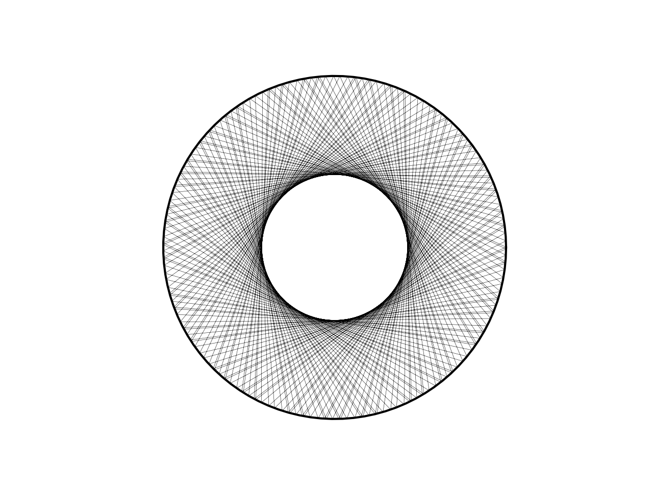
(a)

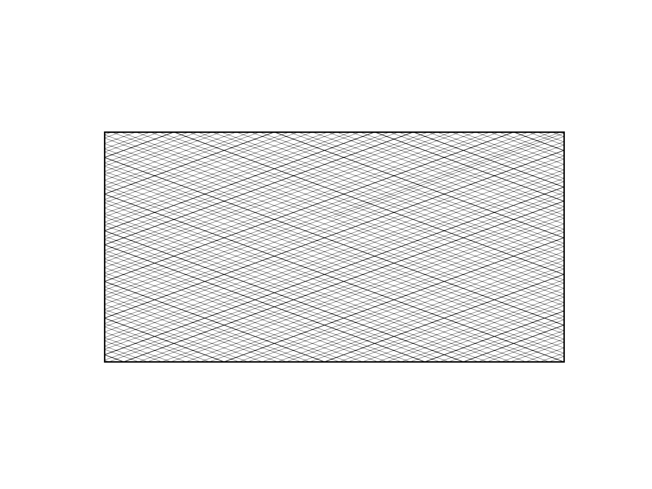
(b)

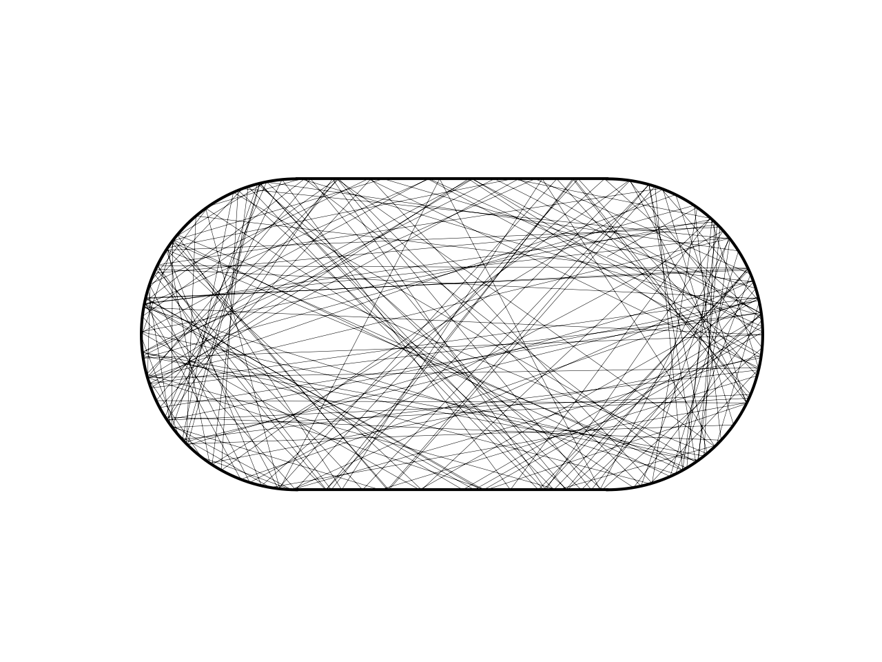
(c)

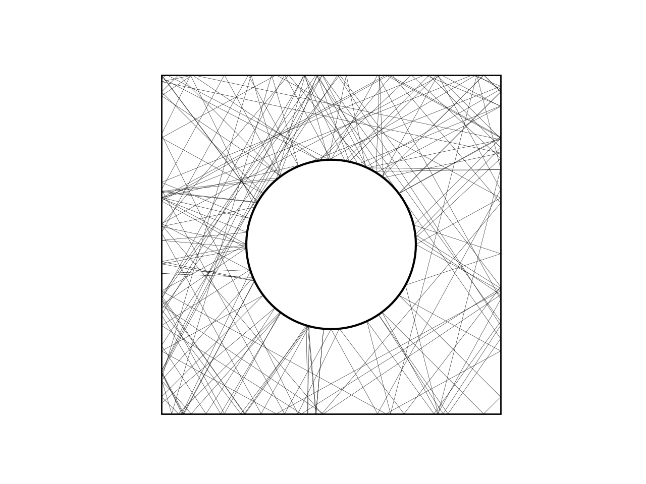
(d)

Figure 2: Trajectories for specular billiards in the circle, rectangle, Bunimovich stadium and Sinai table. This corresponds to setting $\alpha=0$ in eqs.˜7, 8 and 9.

To benchmark our numerics, we now apply the above routine for calculating billiard trajectories to a circular table, a rectangular table and the Bunimovich stadium. It is well-established that in the specular case (see fig.˜2) trajectories are typically regular in the circle and rectangle, and chaotic in the stadium. When plotted in configuration space, it is clear that generic trajectories in the circle and rectangle (figs.˜2(a) and 2(b)) cases are qualitatively more regular than those in the stadium (fig.˜2(c)) (although of course a notable exception is the set of periodic trajectories in the stadium Carlo_2002 ). In the three examples above, this qualitative regularity appears to (anti-)correlate with chaoticity, with the circle and rectangle exhibiting integrable dynamics while the stadium dynamics being chaotic, one might naively expect this correlation to continue into the spinning case. This expectation turns out to be incorrect (see section˜III). However, the dynamics is still sufficiently interesting to warrant a brief discussion of the qualitative regularity of trajectories for spinning billiards.

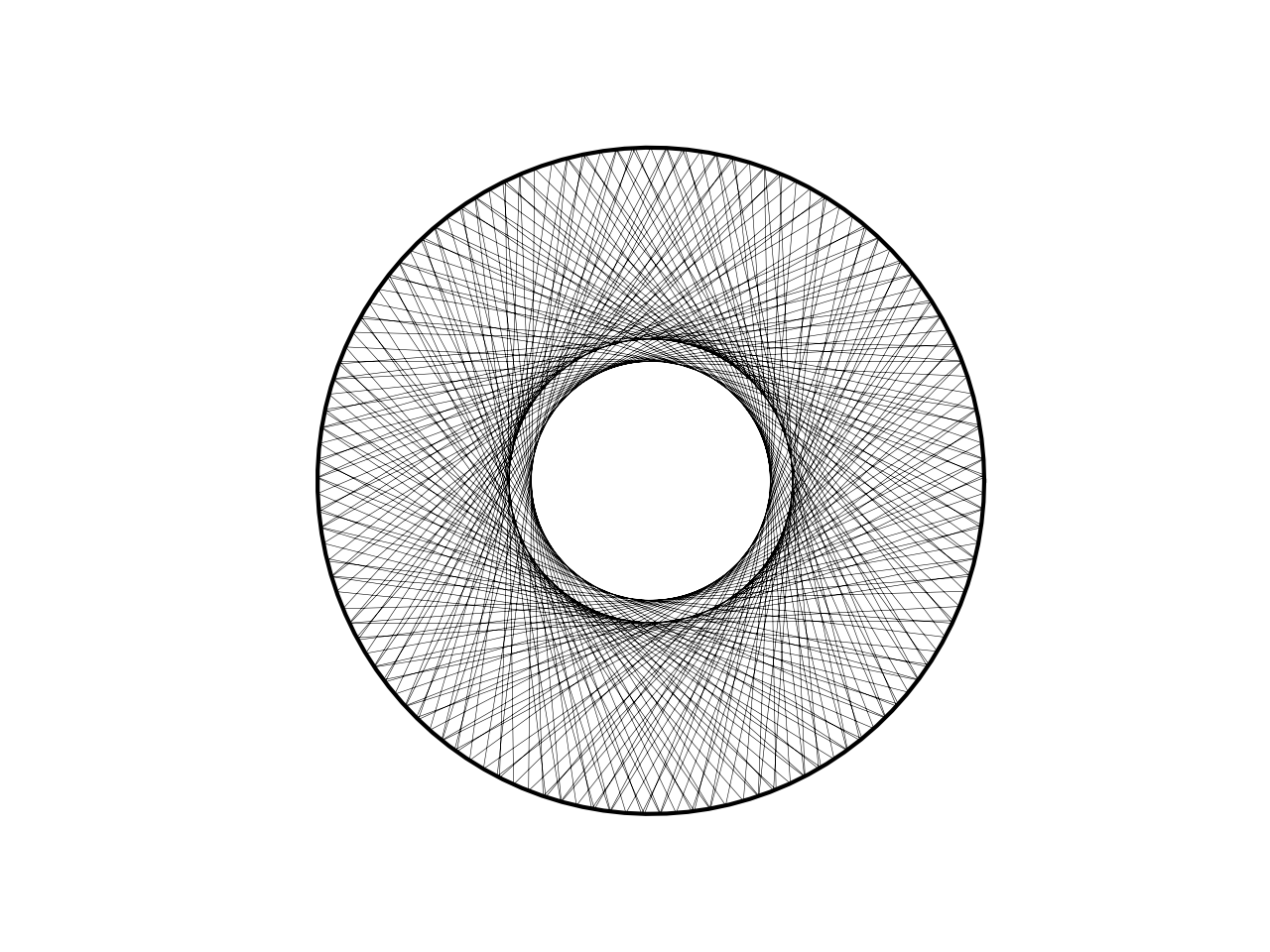
(a) $\alpha=0.1$

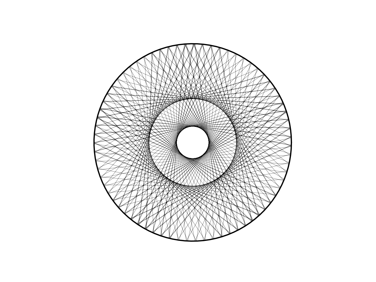
(b) $\alpha=0.5$

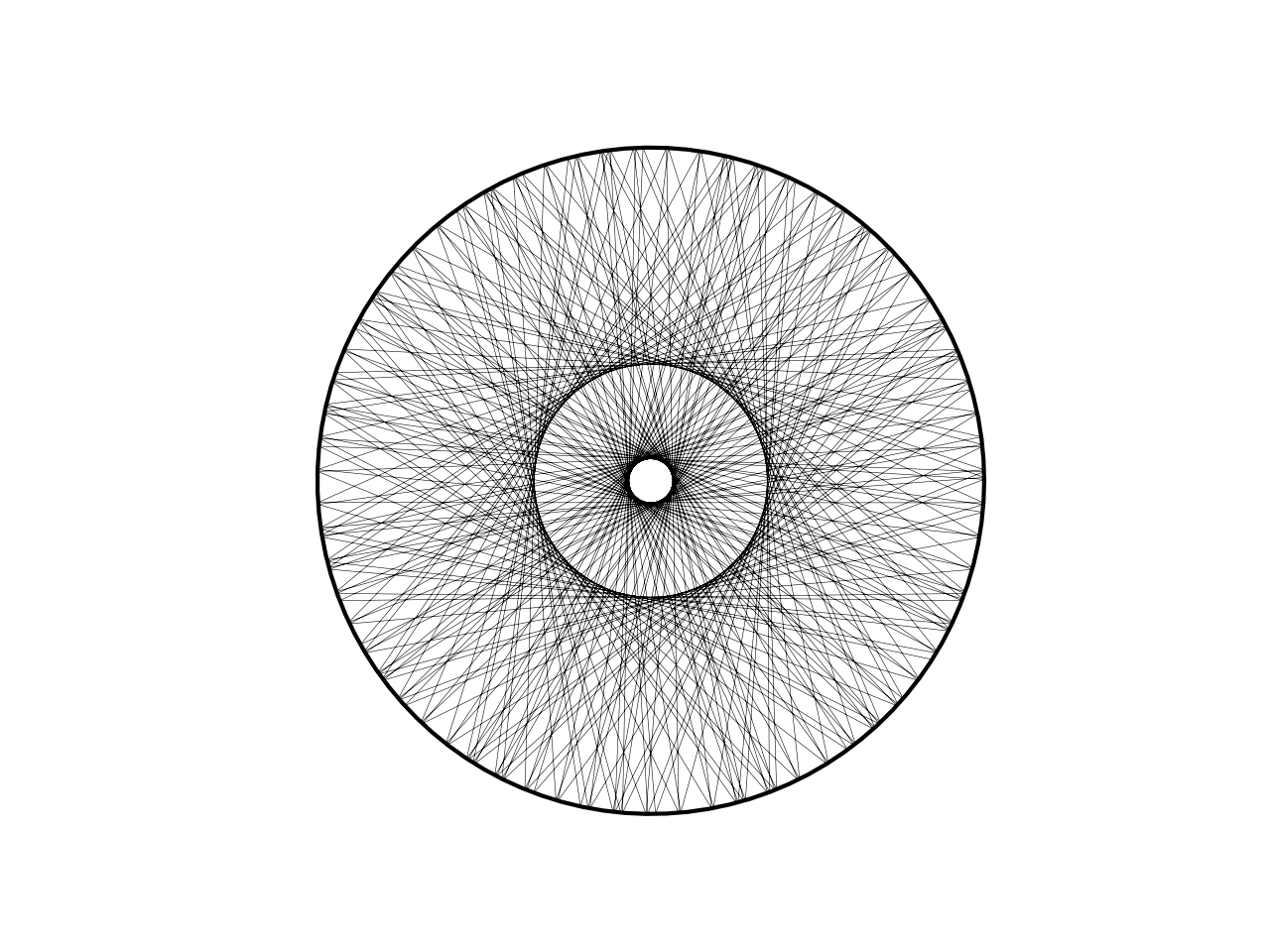
(c) $\alpha=0.7$

Figure 3: Trajectories for spinning billiards on a circular table.

II.3 Circular billiards

In the case of a circular table, all the trajectories for a spinning billiard appear regular, regardless of the initial conditions or value of the moment of inertia coefficient $\alpha$ (fig.˜3). However, while for the specular case, the billiard trajectory traces out a single circular envelope, concentric with the table (fig.˜2(a)), in the spinning case, the pattern of trajectories is more intricate. In particular, the pattern itself qualitatively depends on $\alpha$ and two circular envelopes may be traced out as $\alpha$ increases from 0 to 1 (see in particular fig.˜3(c)).

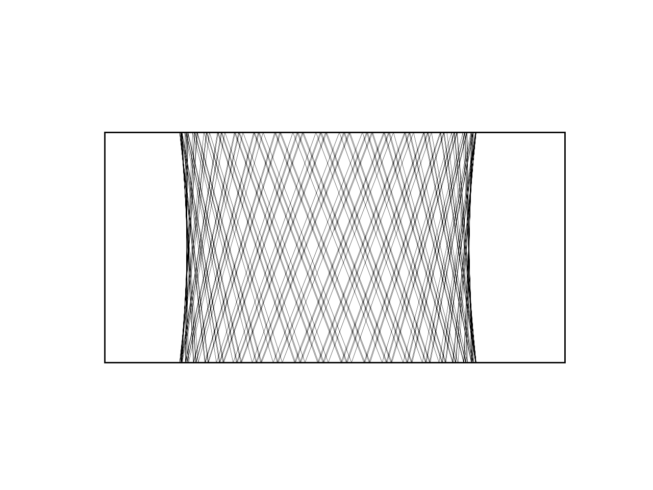
(a) $\alpha=0.1$

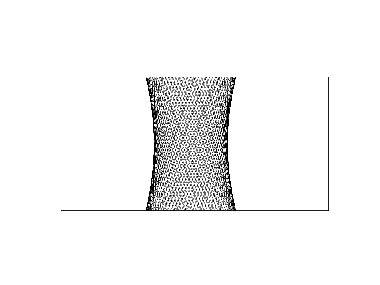
(b) $\alpha=0.5$

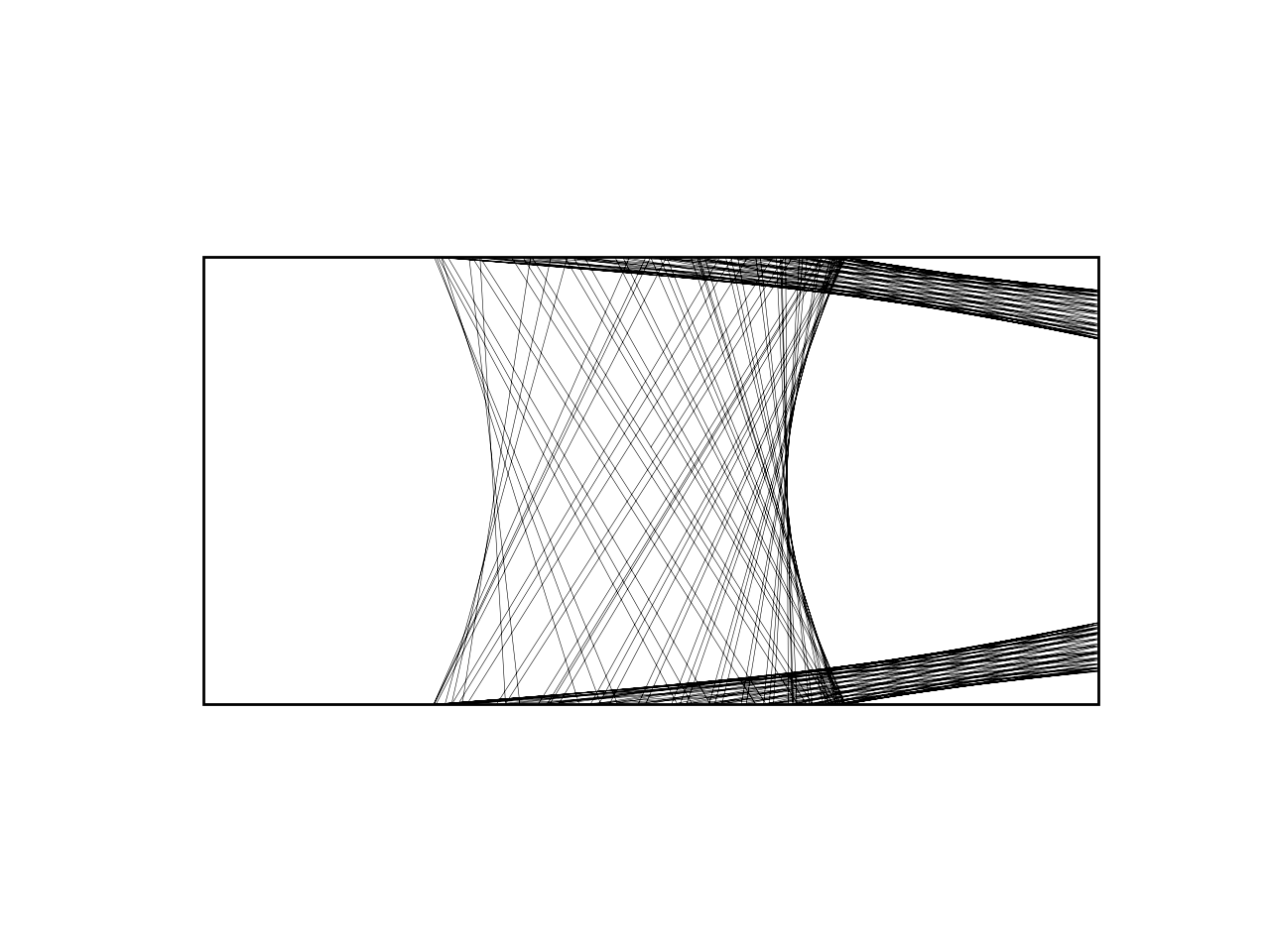
(c) $\alpha=0.7$

Figure 4: Regular-appearing trajectories for spinning billiards in the rectangle table for increasing $\alpha$.

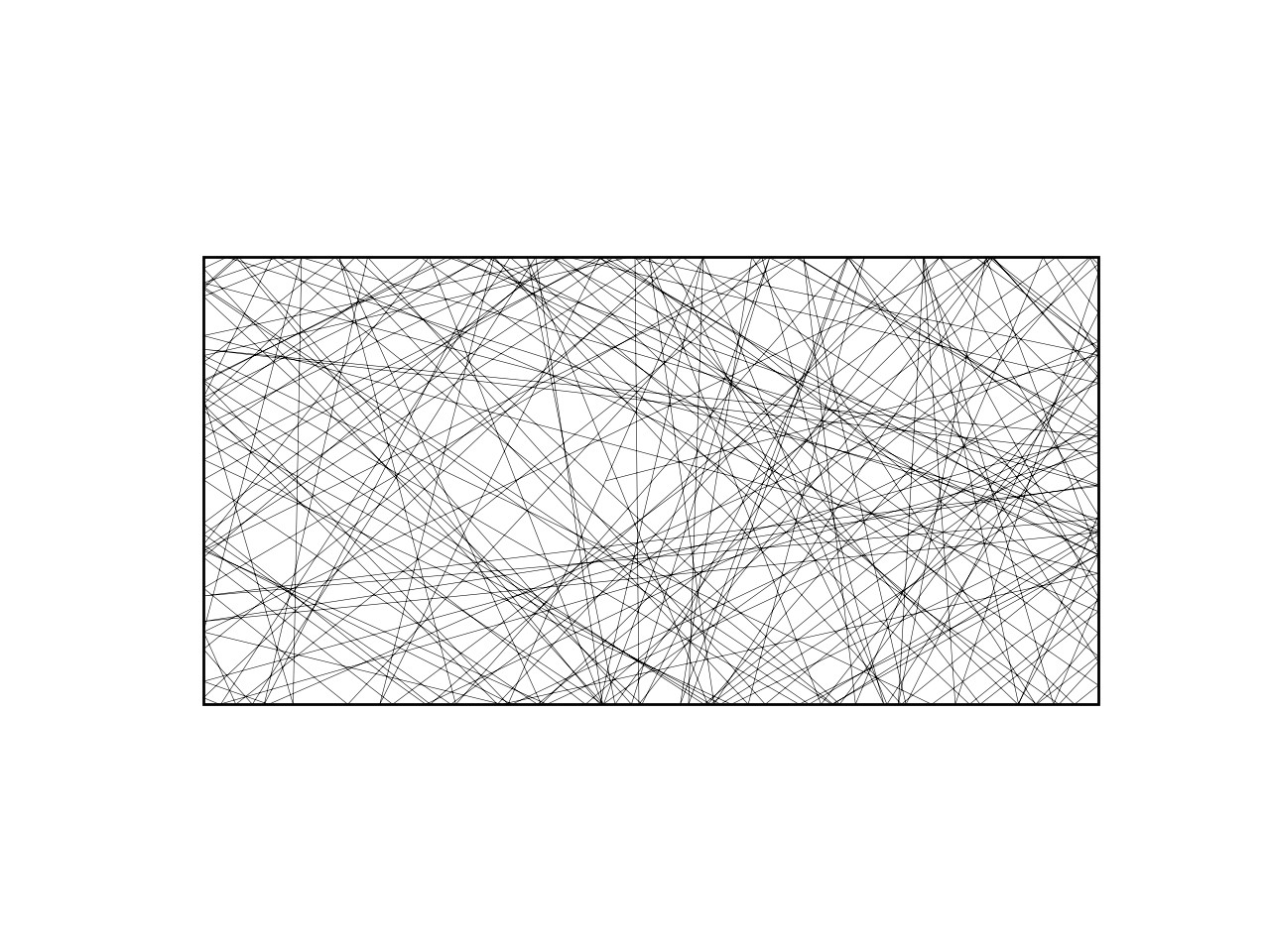
(a) $\alpha=0.1$

(b) $\alpha=0.5$

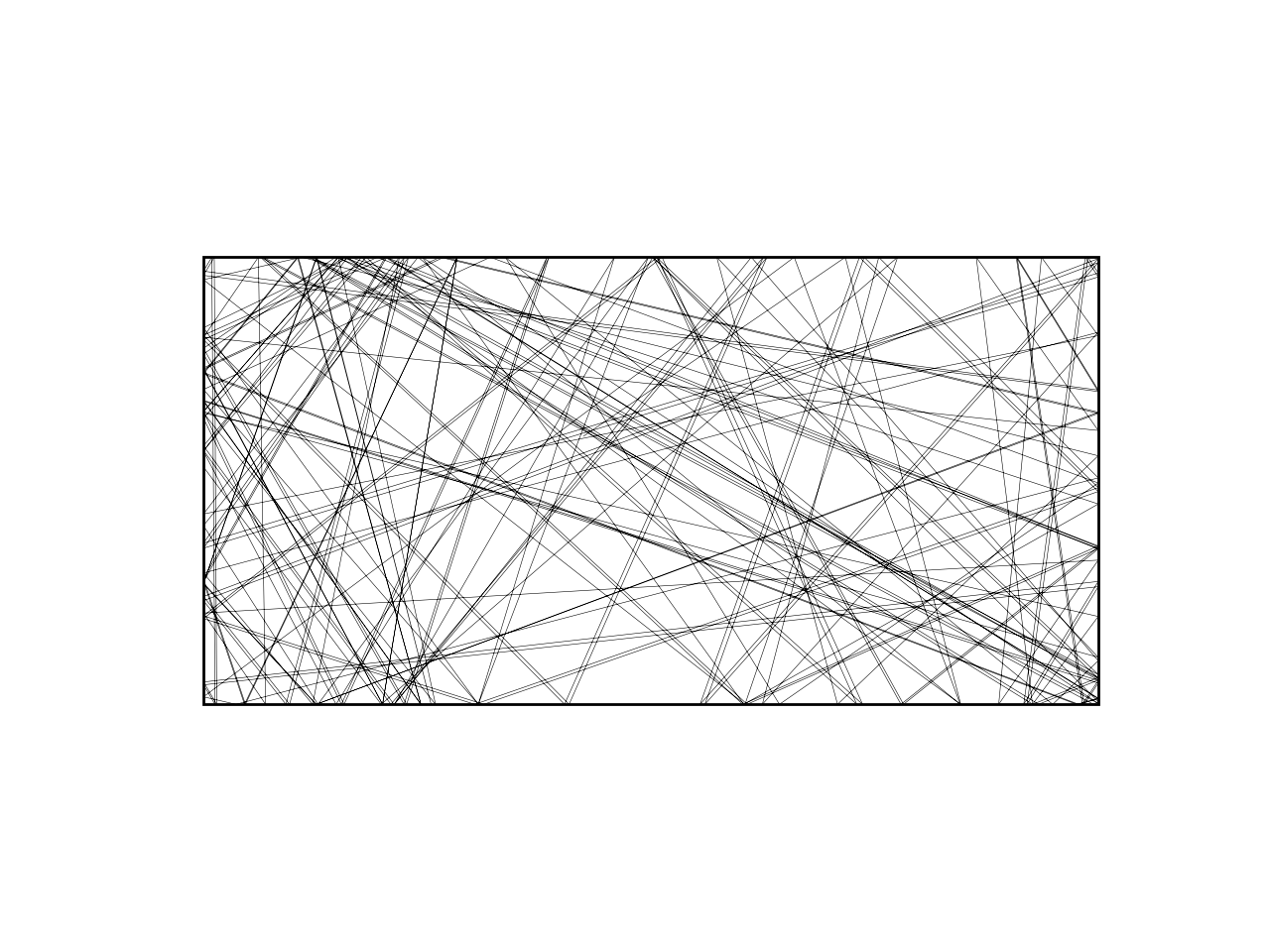
(c) $\alpha=0.7$

Figure 5: Irregular-appearing trajectories for spinable billiards in the rectangle.

II.4 Rectangular billiards

Unlike the specular case, trajectories in the rectangular table either fall into a regular-appearing regime (fig.˜4) or an irregular-appearing regime (fig.˜5), depending on the initial conditions. Of these, the regular-apearing trajectories make up a significant fraction of the phase space of the rectangular spinning billiard, as might be expected. More surprising is the novel set of irregular-appearing trajectories that we report in fig.˜5. Such trajectories as those in figs.˜5(a) and 5(b), which only interact with two opposite sides of the rectangle, are impossible in the non-spinning case, because eq.˜2 implies that the component of the billiard ball’s velocity parallel to the opposite edges will remain constant until it interacts with another wall. It is also worth noting that it is possible for regular-appearing trajectories which interact with other sides of the rectangle to occur (see fig.˜4(c)). We refer the interested reader to Ahmed_2022 and especially the beautifully crafted argument in cox2016stability for more discussion regarding the stability of regular trajectories.

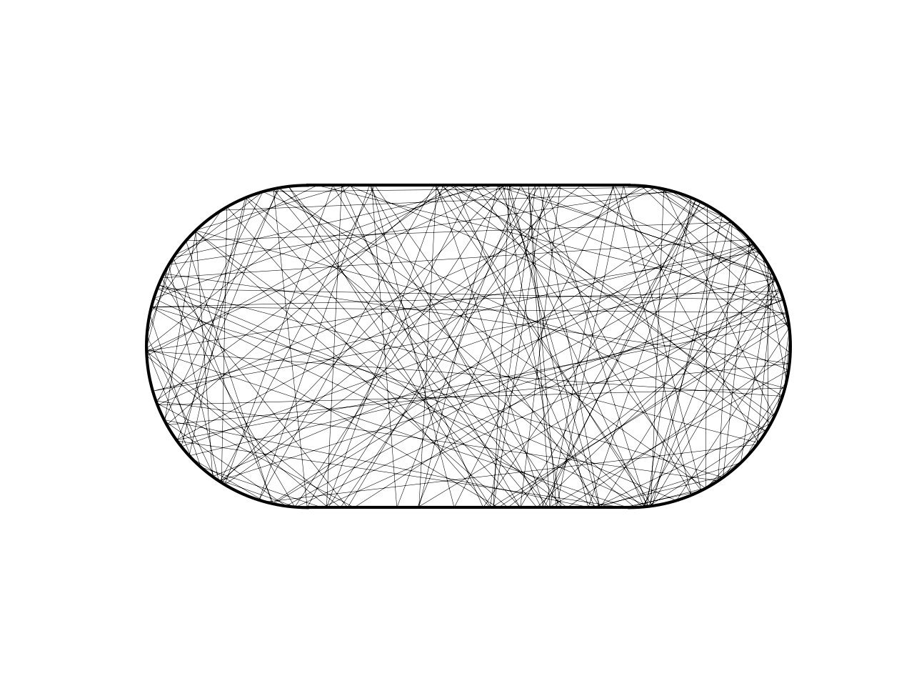
(a) $\alpha=0.1$

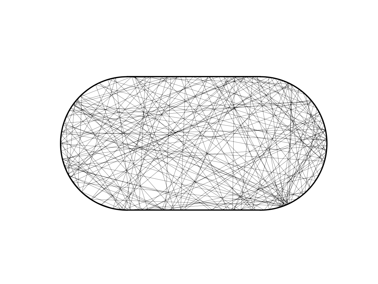
(b) $\alpha=0.5$

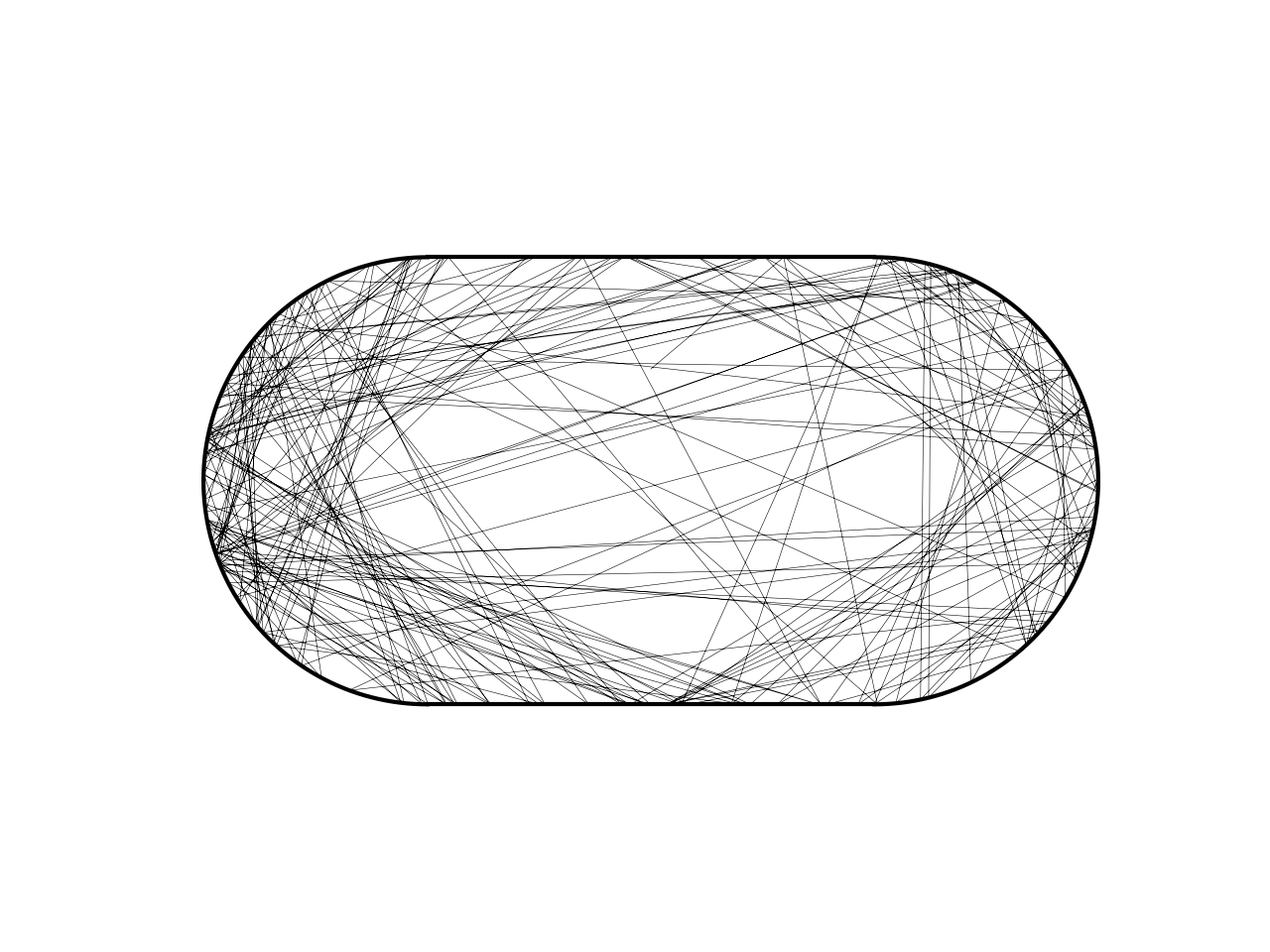
(c) $\alpha=0.7$

Figure 6: Trajectories for spinning billiards in the Bunimovich stadium with increasing $\alpha$.

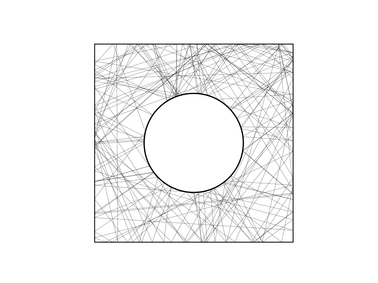
(a) $\alpha=0.1$

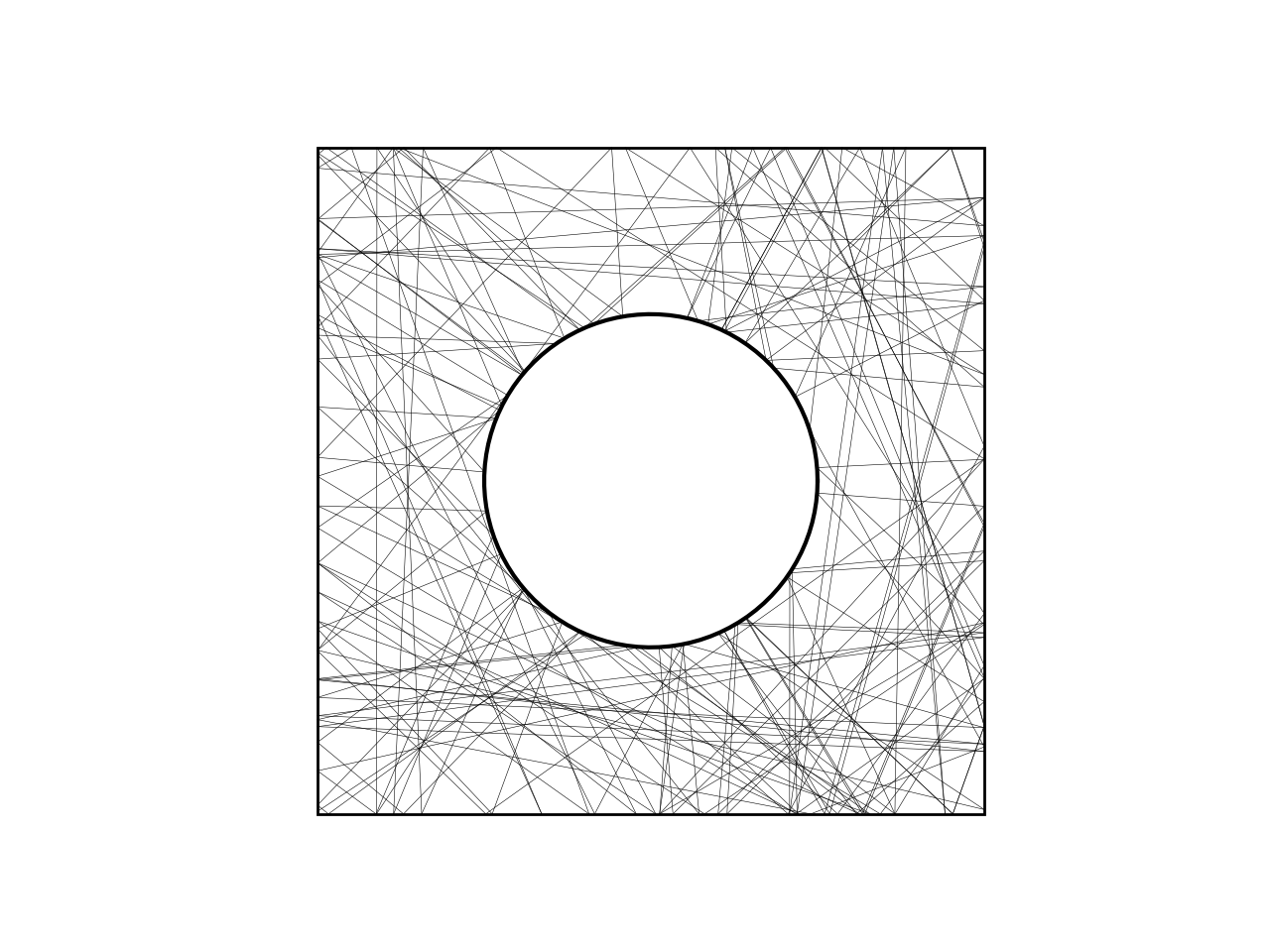
(b) $\alpha=0.5$

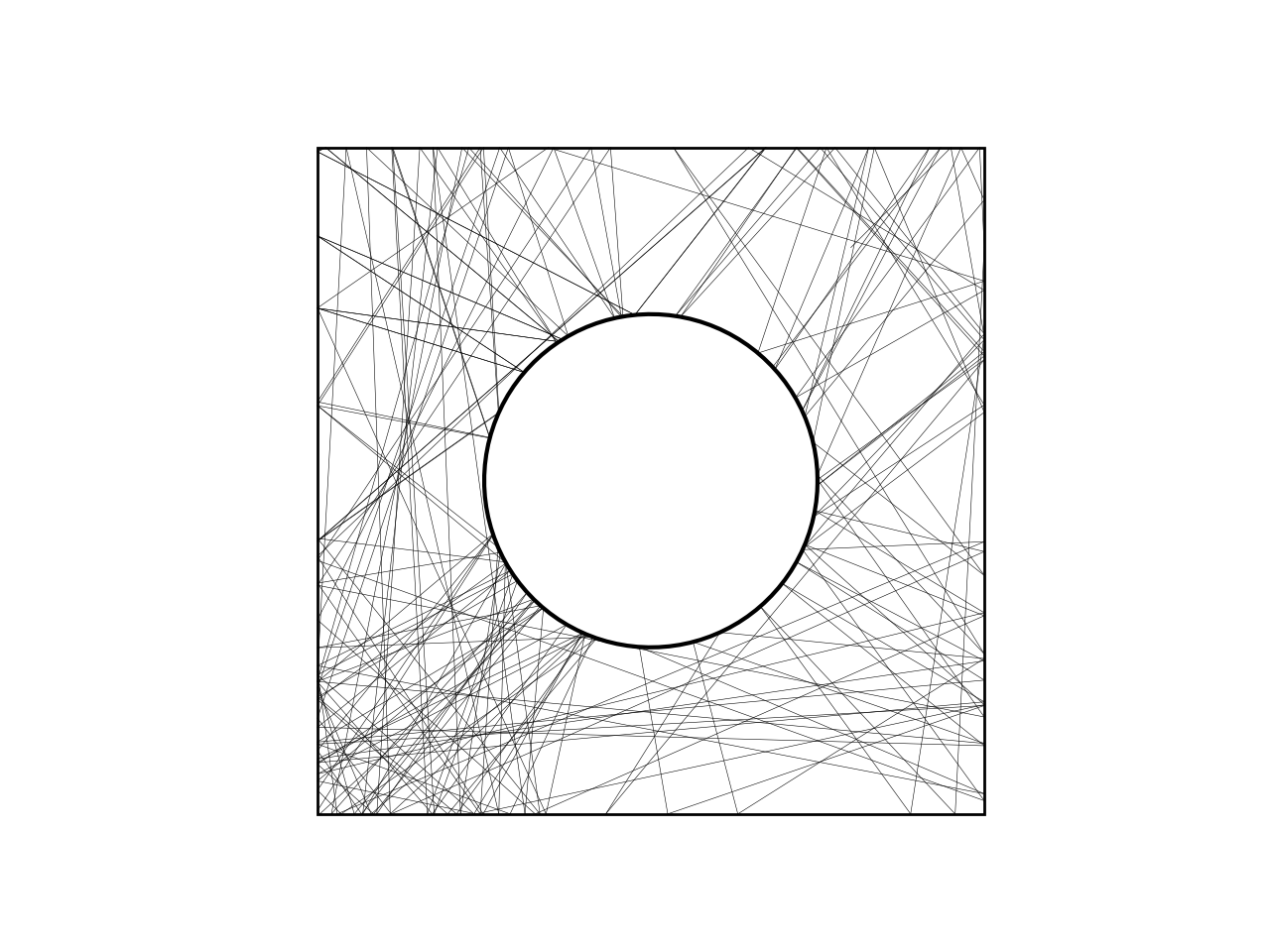
(c) $\alpha=0.7$

Figure 7: Trajectories for spinable billiards on the Sinai table.

II.5 Stadium billiards

As in the case of rectangular billiards, trajectories in the stadium (fig.˜6) fall into a regular-appearing or irregular-appearing regime. However, unlike in the rectangle, the only regular-appearing trajectories are those which interact with the two parallel sides at the top and bottom of the stadium. All trajectories which interact with the semicircular ends of the stadium are irregular-appearing.

II.6 Sinai billiards

Finally, we study Sinai billiard table (fig.3b) consisting of a square table from which a circular region is removed and with reflective conditions imposed on both the inner and outer boundaries. This is one of the most well-known examples of a classical chaotic system. Unlike any of the previous cases, here there are no regular-appearing trajectories for any value of the parameter $\alpha$ other than those which are confined to a region of the table which does not intersect the central circle.

III Lyapunov exponent

Having given a qualitative description of the impact of spin on billiard trajectories, we would like to now give a more quantitative characterisation. One way of doing this is via the Lyapunov exponent or, more precisely, the leading exponent in the Lyapunov spectrum. In order to characterise the chaotic properties of the Bunimovich stadium, it is useful to introduce a parameter, $a$, which represents the length of the rectangular portion of the stadiumPhysRevA.17.773 . Consequently, $a=0$ corresponds to the integrable case of the circular billiard and $a\to\infty$ the integrable parallel plate billiard. For every finite value of $a$, the geometry of the billiard table is a chaotic stadium. The Lyapunov exponent is typically calculated for values of $a$ away from $a=0$ in order to investigate the degree to which the change in boundary conditions introduces chaos in the system. In this article, we are more concerned with how internal properties of the probe affect the chaos properties of the system, and so instead investigate how varying $\alpha$ away from 0 at fixed $a$ affects the Lyapunov exponent $\lambda$.

Following Ose68 ; PhysRevA.17.773 , the LCN can be defined generally for a table $Q$ taken to be a compact connected region of the plane with differential boundary $\partial Q$. We can hence consider the path of the billiard as a flow $\sigma_{t}$ on the manifold with boundary $Q\times\mathbb{R}^{3}$ (here, $\mathbb{R}^{3}$ accounts for the degrees of freedom in the $x$ and $y$ components of velocity, as well as the spin). Let $|Q|$ denote the area of $Q$. Note that the Liouville measure

$$\textrm{d}\mu\equiv\frac{1}{2\pi|Q|}\textrm{d}x\textrm{d}y\textrm{d}v_{x}\textrm{d}v_{y}\textrm{d}u$$ (10)

is invariant under $\sigma_{t}$. It can hence be shown Ose68 that for $\mu$-almost any $x\in M$ and any non-zero tangent vector $e\in T_{x}M$, the limit

$$\lim_{\begin{subarray}{c}t\rightarrow\infty\\ \sigma_{t}(x)\not\in\partial M\end{subarray}}\frac{1}{t}\ln{||\textrm{d}\sigma_{t,x}(e)||}\equiv\lambda(x,e)$$ (11)

exists and is well-defined (here, $\textrm{d}\sigma_{t,x}:T_{x}M\rightarrow T_{\sigma_{t}(x)}M$ is the pushforward of $\sigma_{t}$). Moreover, for almost any $e\in T_{x}M$, $\lambda(x,e)$ attains a non-negative maximal value $\lambda_{\textrm{max}}(x)$.

In order to compute $\lambda_{\textrm{max}}(x)$, we follow PhysRevA.14.2338 ; PhysRevA.17.773 , which is based on the approximate identification of a small tangent vector $e\in T_{x}M$ with a small segment of length $\varepsilon=||e||$ in $M$ separating $x$ from some nearby point $y$. Let $\varepsilon(t)$ denote the length of the segment between $\sigma_{t}(x)$ and $\sigma_{t}(y)$. Then, for any $t$ such that $\varepsilon(t)$ is sufficiently small, we have $\varepsilon(t)\approx||\textrm{d}\sigma_{t,x}(e)||$. We then follow the following procedure: after one collision (which takes a time $t_{1}$) we renormalise the segment separating $\sigma_{t_{1}}(x)$ and $\sigma_{t_{1}}(y)$ with a segment of length $\varepsilon$ starting at $\sigma_{t_{1}}(x)$. Thus, in terms of the reduction factor $\beta_{1}\equiv\frac{||e||}{\varepsilon(t_{1})}$, the time-evolved length $\varepsilon^{(1)}(t)$ of the renormalised segment is $\varepsilon^{(1)}(t)\approx\beta_{1}||\textrm{d}\sigma_{t,x}(e)||$. This procedure can then be repeated for any given number $n$ of collisions, where the time-evolved length $\varepsilon^{(n)}(t)$ of the segment which orginated at $\sigma_{t_{n}}(x)$ is given by:

$$\varepsilon^{(n)}(t)\approx\beta_{1}...\beta_{n}||\textrm{d}\sigma_{t,x}(e)||$$ (12)

Here, $t$ must be between the total time after the $n$-th collision and the total time before the $(n+1)$-th collision (i.e. $\sum_{i=1}^{n}t_{i}\leq t\leq\sum_{i=1}^{n+1}t_{i}$). From this, the parameter

$$k_{t}(x,\varepsilon)=-\frac{1}{t}\sum_{i=1}^{n}\ln\beta_{i}\approx\frac{1}{t}\ln{\frac{||\textrm{d}\sigma_{t,x}(e)||}{||e||}}$$ (13)

can be calculated. If $\varepsilon$ is sufficiently small, then in the large $t$ limit, $k_{t}(x,\varepsilon)$ tends to $\lambda_{\textrm{max}}(x)$ independently of the direction and magnitude of the initial separation PhysRevA.17.773 .

By now, there are a number of ways to compute $\lambda$, some more computationally efficient than others, depending on the system in question. For the purposes of our billiard systems, we follow the routine articulated in Ose68 ; PhysRevA.14.2338 ; PhysRevA.17.773 to calculate the Lyapunov characteristic number (LCN). Briefly, the computation is captured by the following algorithm:

1. Start with a vector describing initial conditions $\vec{x}$ and a specified magnitude of perturbation $\varepsilon$.

2. Randomly generate a second vector $\vec{y}$, such that $||\vec{x}-\vec{y}||=\varepsilon$, to act as the perturbed starting point.

3. Evolve both $\vec{x}$ and $\vec{y}$ for one collision. We expect them to have diverged by some amount if the system is chaotic, and hence $||\vec{x}-\vec{y}||>\varepsilon$.

4. Calculate the reduction factor $\beta=\frac{\varepsilon}{||\vec{x}-\vec{y}||}$ and record it.

5. Renormalise by setting $\vec{y}_{\textrm{new}}=\vec{x}+\beta(\vec{y}-\vec{x})$.

6. Repeat steps 3, 4 and 5, storing $\beta$ at each step.

7. Calculate the LCN as $\lambda=-\frac{1}{t}\sum\ln(\beta_{i})$

If the system is chaotic, the LCN will tend towards a fixed, non-zero value at late times . Specifically, in the unspinable case ($\alpha=0$), the LCN tends to zero at late times in the circle and rectangle, and converges to a fixed, non-zero value in the stadium. This affirms the well-known result that billiard trajectories are non-chaotic in the circle and rectangle, and chaotic in the stadiumOse68 . Note that for the spinning billiard, the LCN tends to zero at late times in the circle, rectangle and stadium in both the regular-appearing and irregular-appearing regimes. This suggests that in these three billiard tables, spinning billiards are non-chaotic regardless of regime!

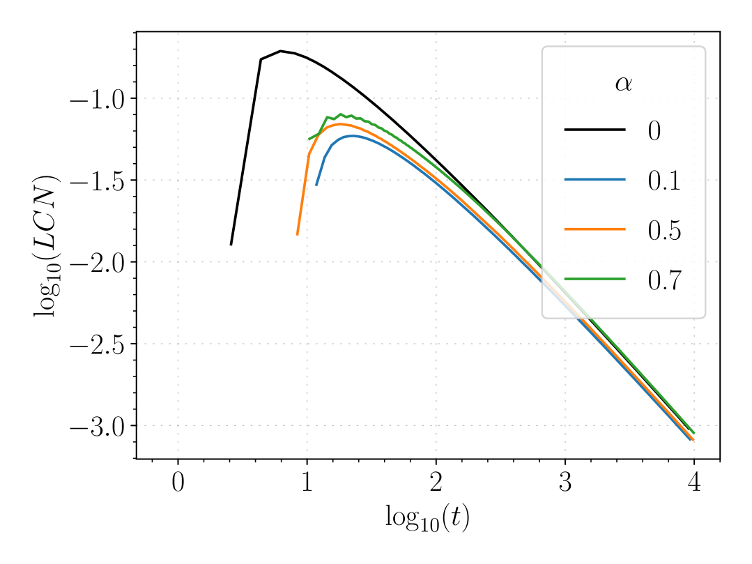
(a) Circle

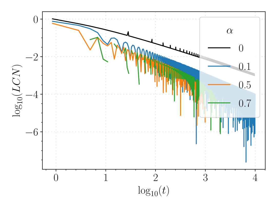
(b) Rectangle

Figure 8: LCN vs time for spinable billiards in the regular regime (see figs.˜3 and 4) in the circle and rectangle.

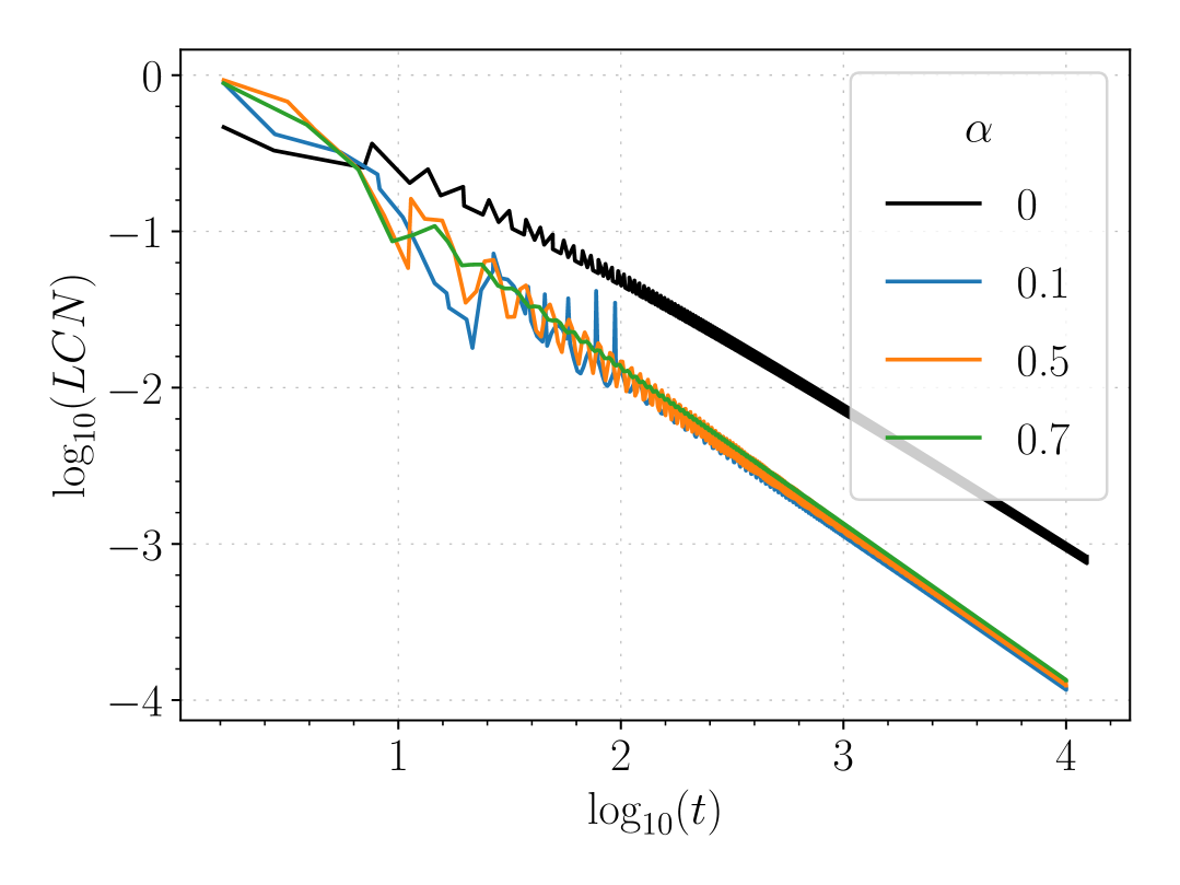
(a) Rectangle

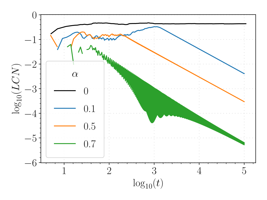
(b) Stadium

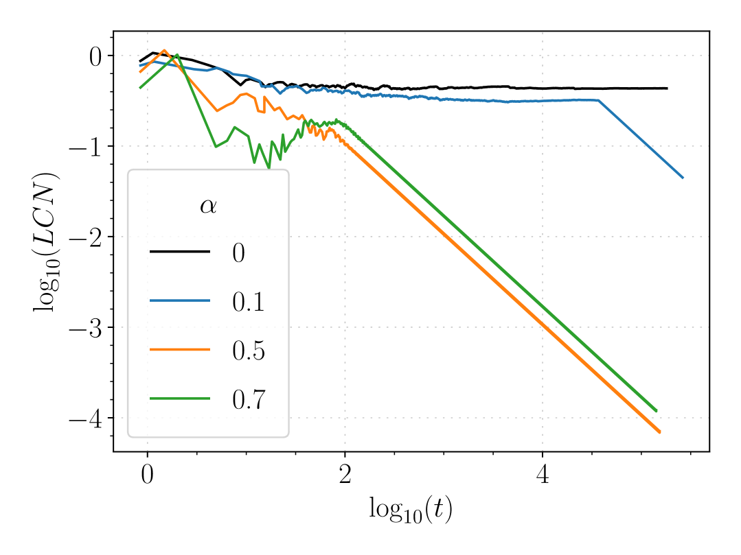
(c) Sinai

Figure 9: LCN vs time for spinable billiards in the irregular regime (see figs.˜5 and 6) in the rectangle, stadium and Sinai table.

IV Separation of phase space variables

Note that rather than describing this system (eqs.˜7, 8 and 9) as a continuous dynamical system on the interior of the billiard table, one could describe it as a discrete dynamical via its Birkhoff map Fierobe2024 . In this discrete system, there are three phase space variables: the position $s$ along the boundary, the angle $\theta$ to the tangent of the boundary at the point of collision and the spin $u$. Because $s$ and $\theta$ are both periodic, the phase space is topologically $S^{1}\times S^{1}\times\mathbb{R}$. As a result, the system can be described by a map $T:S^{1}\times S^{1}\times\mathbb{R}\rightarrow S^{1}\times S^{1}\times\mathbb{R}$.

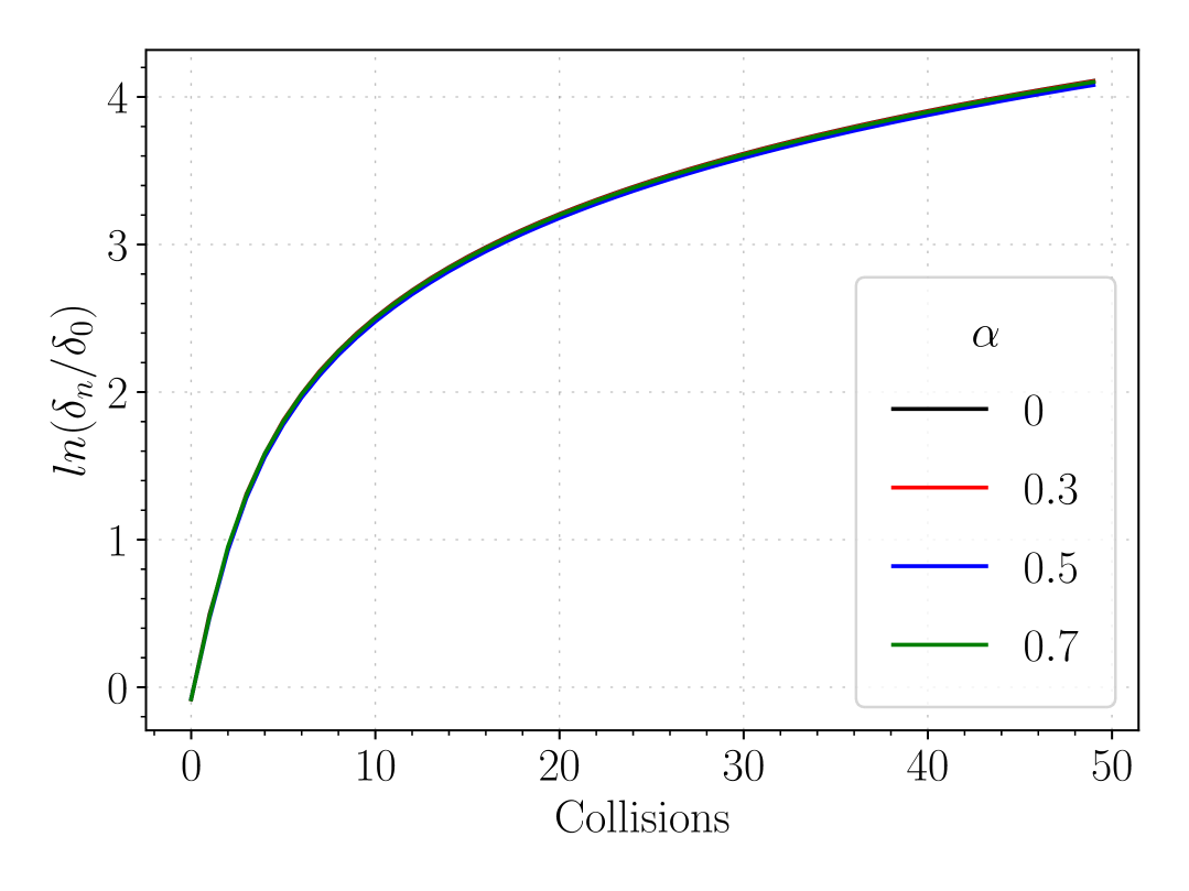
(a) Circle

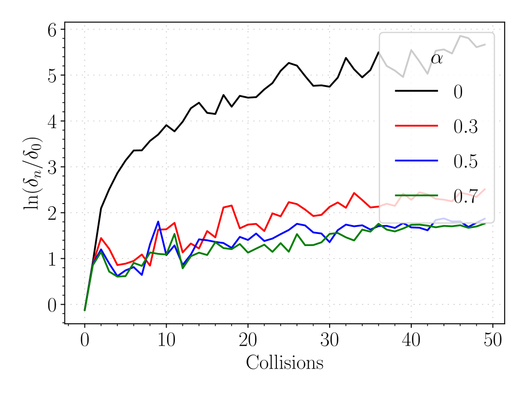
(b) Rectangle

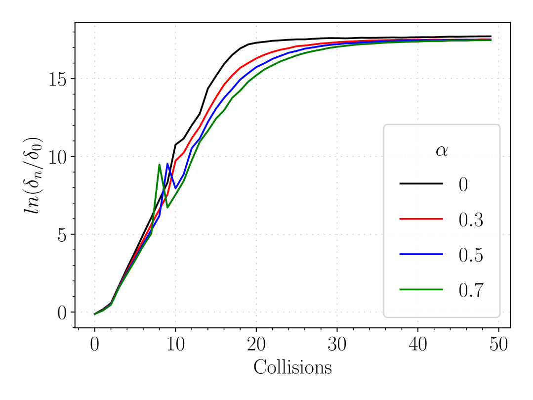
(c) Stadium

Figure 10:

In order to affirm the result given by the Lyapunov exponent suggesting that spinning billiards are non-chaotic in all regimes, we examine how phase space variables separate over time. In particular, fig.˜10 depicts $\log(\delta_{n}/\delta_{0})$, where $\delta_{n}$ is the norm of the separation vector between a trajectory and a perturbation away from it after $n$ collisions averaged over a 8000 different initial conditions in the irregular-appearing regime. It is worth noting that even though $S^{1}\times S^{1}\times\mathbb{R}$ is non-compact, any trajectory is confined within a compact region of phase space. This is because the total spin $u$ attainable in a given trajectory is constrained by the initial energy of the billiard. Thus, the set of possible values for $\ln(\delta_{n}/\delta_{0})$ is bounded and hence, over time the value of $\ln(\delta_{n}/\delta_{0})$ must saturate. This has no bearing on the calculation of the Lyapunov exponent, because of the periodic renormalisation which occurs during the course of its calculation.

In both the circle (fig.˜10(a)) and rectangle fig.˜10(b) it is clear that $\ln(\delta_{n}/\delta_{0})$ evolves logarithmically in both the spinning and non-spinning regime. This aligns with our understanding that these regimes are regular regardless of spin. For the stadium (fig.˜6), it is less clear to see whether $\ln(\delta_{n}/\delta_{0})$ grows linearly or logarithmically from the outset, particularly because of the saturation in $\ln(\delta_{n}/\delta_{0})$ which occurs at later times. This is reflected in the computation of the LCN fig.˜9(b) which evidently needs to be calculated to a fairly late time, before it becomes clear that it will tend to zero in the limit, indicating logarithmic growth of $\ln(\delta_{n}/\delta_{0})$.

V Conclusions

In this work, we have explored the dynamical consequences of endowing classical billiards with internal spin, extending the conventional point-particle approximation by introducing a finite moment of inertia parametrized by a dimensionless constant, $\alpha$. Through detailed numerical investigations across integrable and chaotic billiard geometries—including circular, rectangular, stadium, and Sinai tables—we have shown that spin fundamentally alters the structure of phase space trajectories. Strikingly, our results demonstrate that spinning billiards exhibit an unexpected suppression of chaos. In stark contrast to their non-spinning counterparts, the Lyapunov characteristic number asymptotically vanishes in all geometries studied, including those known to be paradigmatic examples of classical chaos. This finding is further supported by direct analysis of the separation of phase space variables, which shows linear rather than exponential divergence—an indicator of non-chaotic dynamics.

We might ask if there is any good reason to expect a suppression of chaos in the case of spinning billiards. It is clear that with the introduction of spin, there is an additional conserved quantity in our system. For an ideal rigid disk undergoing perfectly elastic, no-slip impacts with a flat wall, the collision law preserves not only the total kinetic energy, but also the “generalised angular momentum” $J+I\omega+mRv_{\parallel}$. Because the wall impulse acts purely along the normal, these two scalars are exact constants of motion at every impact cox2016stability . However, the phase space of the system has been increased by one dimension (when looked at from the point of view of its Birkhoff map), thus leaving the same effective phase space dimension (having applied the additional integral of motion). What can be seen however is that there is a relationship at each collision between linear motion and angular motion, and thus there is a coupling which may be acting to refocus the trajectory at each collision - ie. two trajectories close to each other which would be defocused as described in DETTMANN20092395 in the absence of spin may be refocused by the interchange of angular and linear momentum. In the non-spinning case, the velocity of the billiards is constant, and the billiard is free to explore phase space ergodically. In the spinning case, it is not constant, and thus, with the spin and the velocity, there are two new phase space variables. However, the dynamics within these directions is clearly non-ergodic as there is a constraint on the value of both spin and velocity, as imposed by the bound on the angular and kinetic energy of the system.

These observations suggest that internal structure, in the form of spin, can serve as a stabilizing influence, effectively regularizing the dynamics of otherwise chaotic systems. More broadly, this may have implications for understanding transport and ergodicity in physical systems where internal degrees of freedom are non-negligible, such as in granular flows, soft matter, or even astrophysical systems with extended bodies. It also raises intriguing questions for quantum analogs, where spin could influence quantum chaos, level statistics, or scarring.

Future directions of research along these lines include a more complete classification of the phase space structure, exploration of mixed-spin ensembles, and the potential extension to relativistic and dissipative systems. It would also be of interest to study whether this suppression of chaos persists under stochastic perturbations or in higher dimensions. Clearly, the interplay between geometry, spin, and chaos opens a rich arena for further theoretical and numerical exploration.

- [1] J. Ahmed, C. Cox, and B. Wang. No-slip billiards with particles of variable mass distribution. Chaos: An Interdisciplinary Journal of Nonlinear Science, 32(2), February 2022.
- [2] G. Benettin, L. Galgani, and J. M. Strelcyn. Kolmogorov entropy and numerical experiments. Phys. Rev. A, 14:2338–2345, Dec 1976.
- [3] G. Benettin and J. M. Strelcyn. Numerical experiments on the free motion of a point mass moving in a plane convex region: Stochastic transition and entropy. Phys. Rev. A, 17:773–785, Feb 1978.
- [4] Gabriel G Carlo, Eduardo G Vergini, and Pablo Lustemberg. Scar functions in the bunimovich stadium billiard. Journal of Physics A: Mathematical and General, 35(38):7965–7982, September 2002.
- [5] Christopher Cox, Renato Feres, and Hong-Kun Zhang. Stability of periodic orbits in no-slip billiards, 2016.
- [6] R Cross. Bounce of a spinning ball near normal incidence. American Journal of Physics, 73, 10 2005.
- [7] Carl P. Dettmann and Orestis Georgiou. Survival probability for the stadium billiard. Physica D: Nonlinear Phenomena, 238(23):2395–2403, 2009.
- [8] Corentin Fierobe, Vadim Kaloshin, and Alfonso Sorrentino. Lecture Notes on Birkhoff Billiards: Dynamics, Integrability and Spectral Rigidity, pages 1–57. Springer Nature Switzerland, Cham, 2024.
- [9] R Garwin. Kinematics of an ultraelastic rough ball. American Journal of Physics, 37, 09 1968.
- [10] V. I. Oseledets. A multiplicative ergodic theorem. characteristic ljapunov exponents of dynamical systems. Trans. Moscow Math. Soc., 19:197–231, 1968.