A Linear Approach to Data Poisoning

Abstract

We investigate the theoretical foundations of data poisoning attacks in machine learning models. Our analysis reveals that the Hessian with respect to the input serves as a diagnostic tool for detecting poisoning, exhibiting spectral signatures that characterize compromised datasets. We use random matrix theory (RMT) to develop a theory for the impact of poisoning proportion and regularisation on attack efficacy in linear regression. Through QR stepwise regression, we study the spectral signatures of the Hessian in multi-output regression. We perform experiments on deep networks to show experimentally that this theory extends to modern convolutional and transformer networks under the cross-entropy loss. Based on these insights we develop preliminary algorithms to determine if a network has been poisoned and remedies which do not require further training.

1 Introduction

With foundation models set to underpin critical infrastructure from healthcare diagnostics to financial services, there has been a renewed focus on their security. Specifically, both classical and foundational deep learning models have been shown to be vulnerable to backdooring, where a small fraction of the data set is mislabelled and marked with an associated feature (Papernot et al., 2018; Carlini et al., 2019; He et al., 2022; Wang et al., 2024). If malicious actors exploit these vulnerabilities, the consequences could be both widespread and severe, undermining the reliability of foundation models in security-sensitive deployments.

Recent work has revealed diverse and increasingly sophisticated backdooring strategies. Xiang et al. (2024) insert hidden reasoning steps to trigger malicious outputs, evading shuffle-based defences. Li et al. (2024) modify as few as 15 samples to implant backdoors in LLMs. Other approaches include reinforcement learning fine-tuning (Shi et al., 2023) and continuous prompt-based learning (Cai et al., 2022). Deceptively aligned models that activate only under specific triggers are shown in Hubinger et al. (2024), while contrastive models like CLIP are vulnerable to strong backdoors (Carlini and Terzis, 2022). Style-based triggers bypass token-level defences (Pan et al., 2024), and ShadowCast introduced in Xu et al. (2024) uses clean-label poisoning to embed misinformation in vision–language models.

Although backdooring in machine learning has been extensively studied experimentally, robust mathematical foundations are still lacking, even for basic models and attack scenarios. This paper introduces a novel mathematical framework for analyzing backdoors in linear regression models.

We motivate the input Hessian in Section 2, derive the spectral signatures for multi-output regression in Section 3, peform a comprehensive RMT analysis of poison efficacy for regression in Section 4 and perform extensive supporting experiments in Section 5, mentioning a defence algorithm that is detailed in Appendix B. We also release a software package alongside the paper for experimental calculation of the input Hessian.

2 Motivation

Previous works Tran et al. (2018); Sun et al. (2020) argue that backdoors introduce sharp outliers in the Hessian spectrum. In contrast, Hong et al. (2022) show that by directly modifying model parameters, their handcrafted backdoors avoid associated sharp curvature, producing up to $100\times$ smaller Hessian eigenvalues. In second order optimisation, the Hessian with respect to the parameters follows by taking a small step and truncating the Taylor expansion. But if we retrain the network with backdoor data poisoning, what mathematical justification do we have to expect that the change in weights should be small , thereby justifying the second order truncation?

However, for certain well-studied experimental types of backdoor data poisoning, such as the small cross from Gu et al. (2017) further detailed in the experimental section, the change in input is small under an appropriate norm (e.g. $L_{1}/L_{2}$). This mathematically motivates the expansion of the loss with respect to the input

$$L(x+\delta x)=L(x)+\delta x^{T}\nabla_{x}L+\frac{1}{2}\delta x^{T}\nabla^{2}_{\mathbf{x}}L\delta x.$$ (1)

where we anticipate the expectation under the data-generating distribution of the second and/or third terms (and equivalently their sample means) to be large for the poisoned model but small for the clean model.. This motivates the study of the gradient and Hessian with respect to the input,

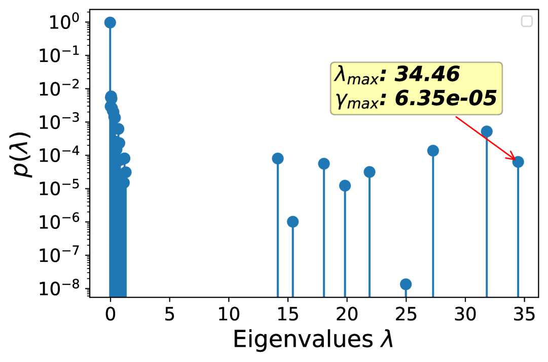
(a) Poisoned ESD $\nabla^{2}_{\mathbf{w}}L$

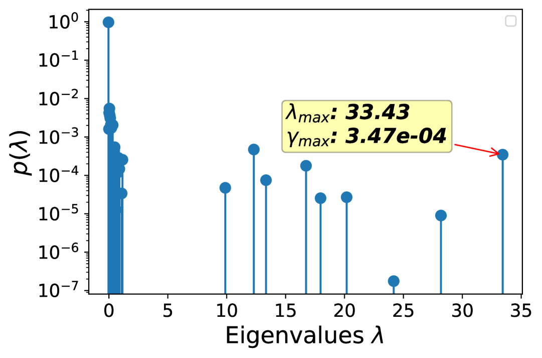
(b) Pure ESD $\nabla^{2}_{\mathbf{w}}L$

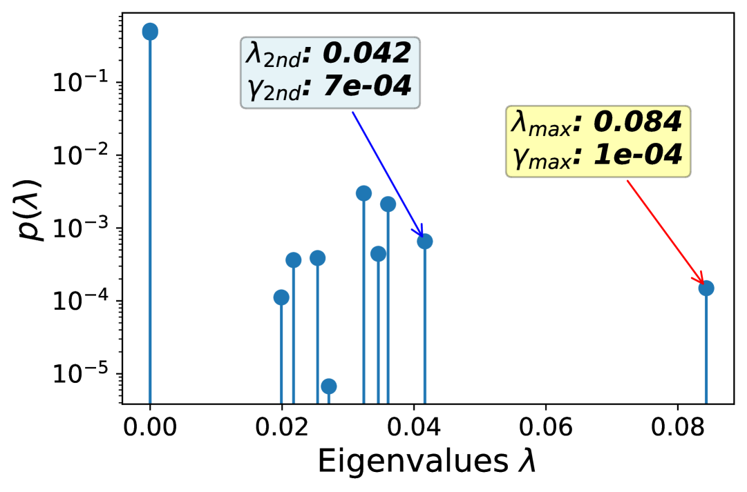
(c) Poisoned ESD $\nabla^{2}_{\mathbf{x}}L$

(d) Unpoisoned ESD $\nabla^{2}_{\mathbf{x}}L$

Figure 1: Logistic Regression MNIST comparison of Poisoned and Unpoisoned (Pure) Networks’ Empirical Spectral Densities (ESD) of the Hessian with respect to the weights/inputs $\nabla^{2}_{\mathbf{w}}L/\nabla^{2}_{\mathbf{x}}L$.

As shown in Figure 1, for logistic regression, we observe only a marginal increase in the spectral norm of the Hessian with respect to the weights under backdoor data poisoning. However, we find a substantially larger increase in the spectral norm of the Hessian with respect to the input.

2.1 Why the Hessian with respect to the weights cannot measure data poisoning

Consider the input data $X\in\mathbb{R}^{n\times p},$ where $x_{i}\in\mathbb{R}^{p}$ is drawn from one of $k$ Gaussian components, each with mean $\mu_{\ell}$ and covariance $\Sigma_{\ell}$. Denote the overall empirical mean ($\bar{x}=\frac{1}{n}\sum_{i=1}^{n}x_{i}$) and cluster mean ($\bar{x}_{\ell}=\frac{1}{n_{\ell}}\sum_{i:z_{i}=\ell}x_{i}$). The sample covariance can then be written as:

$$\underbrace{\sum_{\ell=1}^{k}\sum_{i=1}^{n_{\ell}}(x_{\ell,i}-\bar{x}_{\ell})(x_{\ell,i}-\bar{x}_{\ell})^{\top}}_{\text{Within-Cluster Scatter}}\;+\;\underbrace{\sum_{\ell=1}^{k}n_{\ell}\bigl{(}\bar{x}_{\ell}-\bar{x}\bigr{)}\bigl{(}\bar{x}_{\ell}-\bar{x}\bigr{)}^{\top}}_{\text{Between-Cluster Scatter}},$$

where $z_{i}\in\{1,\dots,k\}$ is the cluster label and $n_{\ell}$ is the number of points in cluster $\ell$. For linear regression, the Hessian is just the unnormalised sample covariance matrix ($X^{T}X$). For large datasets where each class has an appreciable count of examples, $n_{\ell}\approx n/k$ and so we expect up to $k$ outlier eigenvalues Benaych-Georges and Nadakuditi (2011). As the outliers are determined by the between-cluster term, when poisoning a fraction of datapoints $\alpha$ with altered features $x\rightarrow x+\delta x$, the relevant squared term becomes

$$\left|\hat{x}-x_{\ell}-\alpha\delta x\left(1-\frac{1}{k}\right)\right|\leq\left|x_{\ell}\right|+\alpha\left|\delta x\right|$$ (2)

where we use the Cauchy-Schwarz inequality and center the data matrix to $0$. Intuitively, the biggest change in outlier we have would be if the perturbation rests along the vector to centroid mean from the global mean and is again to first order linear in $\alpha$ and $\delta x$. For targeted data poisoning to be a reasonable threat $\alpha\ll 1$ and $|\delta x|\ll|x_{\ell}|$. As such, we can clearly state that for linear regression we do not expect any outliers from targeted data poisoning. Extending to multinomial logistic regression, the Hessian is simply $X^{T}DX$, where

$$(D_{i})_{k\ell}=p_{ik}\bigl{(}\delta_{k\ell}-p_{i\ell}\bigr{)},\qquad\Bigl{[}p_{i\ell}=\tfrac{1-p_{ik}}{K-1}\Bigr{]}\quad\Longrightarrow\quad D=\left(1+\frac{1}{K-1}\right)\mathbf{I}-\frac{1}{K-1}\mathbf{1},$$

and hence, assuming a maximum entropy distribution over the incorrect labels, we have a rank-one update (in reduction of the global mean) to the previously discussed linear-regression solution.

2.2 An intuitive understanding of the Hessian and gradient with respect to the input

In successful targeted data poisoning, the model classifies the target class with high probability $1-\alpha$, while the correct class would be classified with probability approximately $\frac{\alpha}{K-1}$, where $K$ is the class count/alphabet size. The cross entropy loss change $\delta L$ to first order is

$$\delta L=\log(K-1)-\log\alpha\approx\delta x^{T}\nabla_{x}L$$ (3)

For simplicity, let us consider that the minimal perturbation required to achieve this $\delta L$ is a vector with components $\delta x_{i}\in(-\alpha,0,\alpha)$ for some poison strength $\alpha$ equivalent to whiting/blacking out certain pixels for a normalized image. As such, in the set ${\mathcal{S}}=\{(i,j):(\delta x)_{ij}\neq 0\}$ of non zero perturbations $\sum_{(i,j)\in\mathcal{S}}(\nabla_{x}L)_{ij}(\delta x)_{ij}=\delta L$ and therefore

$$\frac{1}{|S|}\sum_{(i,j)\in S}(\nabla_{x}L)_{ij}=\frac{\delta L}{\alpha|S|}$$ (4)

On average, the magnitude of a backdoor gradient element is proportional to its change in loss and inversely proportional to the number of trigger elements/their intensity. As such, we expect the gradient to light up more in trigger areas than in the areas of input that genuinely reflect the data surface. We show this both in our QR analysis Section 3 and RMT analysis 4. For adversarial training, $\nabla_{x}L\approx 0$, thus the change in loss (Equation 3) will be dominated instead by the quadratic term (see experimental fit in 5(a)). In this scenario, denoting $\lambda_{i},\phi_{i}$ for the eigenvalues and eigenvectors of the input Hessian respectively, we have

$$\sum_{i}\lambda_{i}^{poisoned}(\delta x^{T}{\phi_{i}})^{2}=2\delta L.\quad\sum_{i}\lambda_{i}^{pure}(\delta x^{T}{\phi_{i}})^{2}\approx 0.$$ (5)

Assuming that the poison feature $\delta x$ has zero overlap with the outliers of the Hessian with respect to the input, for a large change in loss, there will be a new outlier eigenvector corresponding to $\delta x$. Similarly restricting $\delta x$ to a set of $\mathcal{S}$ elements of magnitude $\alpha$ and the rest zero. Then if $\delta x$ is the movement along $\phi_{i}$ required to get the loss change $\delta L$. Then $\delta x=\sqrt{|\mathcal{S}|}{\phi_{i}}$ and so

$$\lambda_{i}^{poisoned}=\frac{2\delta L}{\alpha^{2}|\mathcal{S}|}$$ (6)

We thus expect backdoor data poisoning to cause new spikes in the Hessian with respect to the input which will be larger than existing spikes.

3 Stepwise regression approach to data backdooring

For linear regression, by stepwise addition of the poison feature for both poisoned and unpoisoned (pure) models, we can analytically derive the difference in solutions. We denote the augmented data matrix $\mathbf{X}_{\text{aug}}\;=\;\bigl{[}\,\mathbf{X},\;\mathbf{x}_{\text{new}}\bigr{]}\;\;\in\;\mathbb{R}^{n\times(p+1)}$, $\beta_{\text{new}}\in\mathbb{R}$ the coefficient of $\mathbf{x}_{\text{new}}$, and $\beta_{i}^{(\text{new})}$ the updated coefficients for the old features $\mathbf{X}$. As derived and detailed in Appendix B, by further including $\mathbf{x}_{\text{new}}$ in the model, the least-squares solution and the decrease in residual square error are

$$\beta_{\text{new}}\;=\;\frac{\,\mathbf{x}_{\text{new}}^{T}\,\mathbf{e}\,}{\,\mathbf{x}_{\text{new}}^{T}\bigl{(}\mathbf{I}-P_{\mathbf{X}}\bigr{)}\mathbf{x}_{\text{new}}\,},\quad\Delta\text{RSS}\;=\;\frac{(\,\mathbf{x}_{\text{new}}^{T}\,\mathbf{e}\,)^{2}}{\,\mathbf{x}_{\text{new}}^{T}\,\bigl{(}\mathbf{I}-P_{\mathbf{X}}\bigr{)}\,\mathbf{x}_{\text{new}}\,},$$

where $\mathbf{e}\;=\;\mathbf{Y}-\mathbf{X}\,\hat{\bm{\beta}}$ and $P_{\mathbf{X}}\;=\;\mathbf{X}\bigl{(}\mathbf{X}^{T}\mathbf{X}\bigr{)}^{-1}\mathbf{X}^{T}.$ After adding $\mathbf{x}_{\text{new}}$, the old coefficients $\hat{\bm{\beta}}$ become $\bm{\beta}^{(\text{new})}$ and the update rule is

$$\bm{\beta}^{(\text{new})}=\hat{\bm{\beta}}-\left[(\mathbf{X}^{T}\mathbf{X})^{-1}\mathbf{X}^{T}\mathbf{x}_{\text{new}}\right]\bm{\beta}_{\text{new}}.$$

Due to the difference in magnitude of $||\mathbf{e}||$ for the poisoned and unpoisoned training sets, we expect very high weight values for the poison features specifically in the weight vector for the poison target variable. We verify these predictions with multi-output regression MNIST (with full details and extensive ablation analysis in Appendix D). We show the impact of poisoning on the class output weights in Fig 2(a), along with extremely precise experimental predictions (Fig 2(c) and 2(d)) of stepwise regression compared to the true retraining change 2(b).

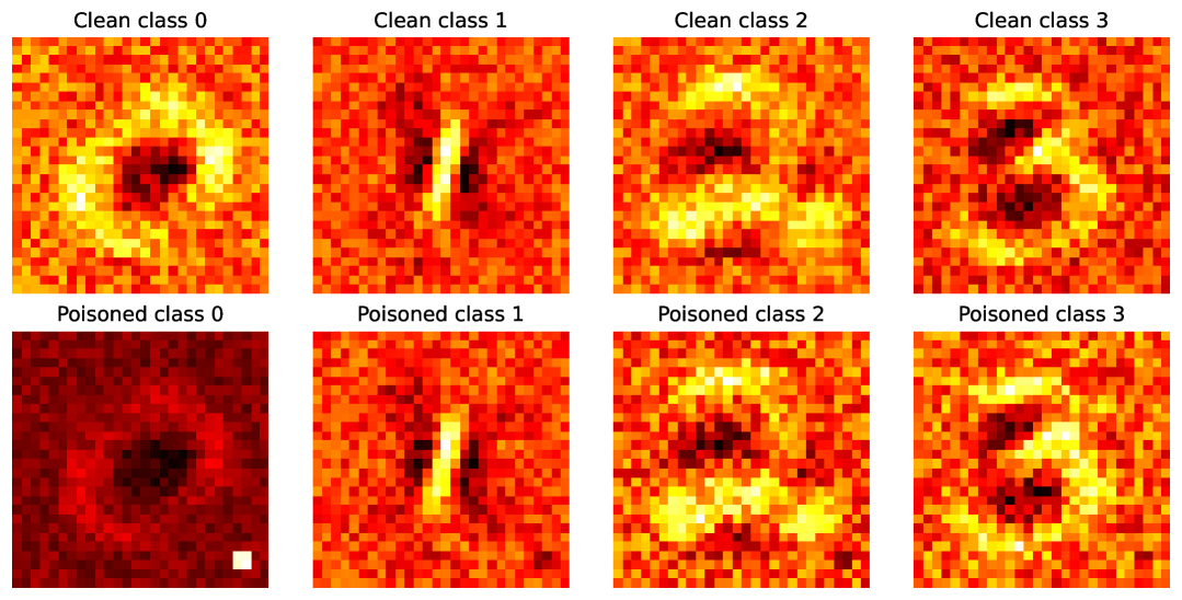
(a) Regression weights per class

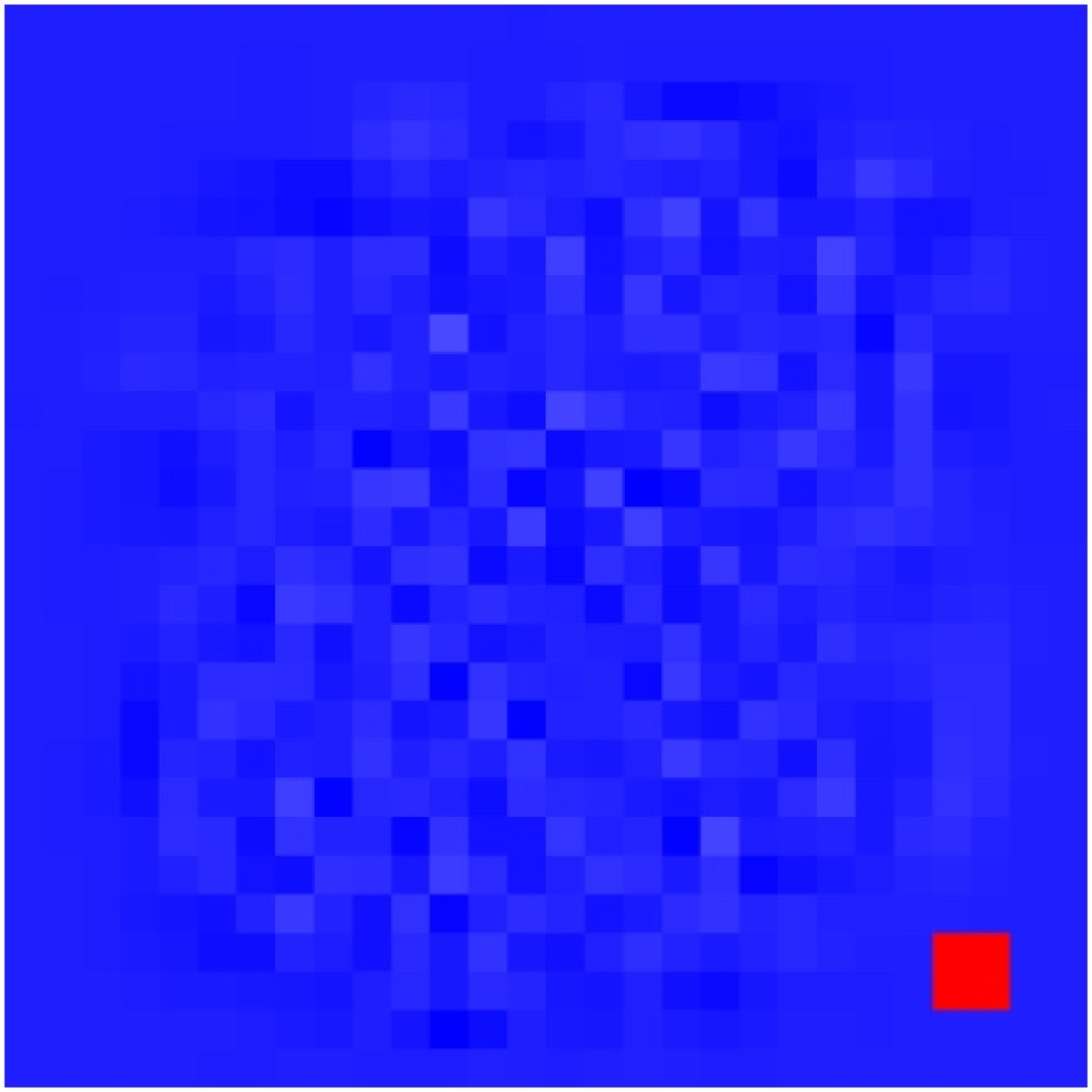
(b) $\Delta\bm{\beta}^{\mathrm{full\;-\;base}}_{c=0}$

(c) $\Delta\bm{\beta}^{\mathrm{step\;-\;base}}_{c=0}$

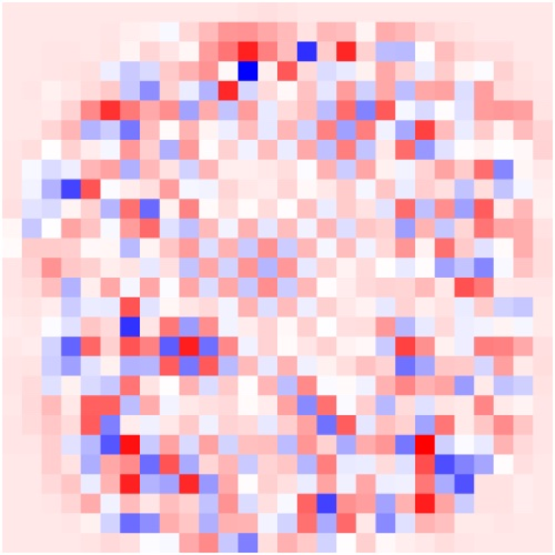
(d) $\Delta\bm{\beta}^{\mathrm{step\;-\;full}}_{c=0}$

Figure 2: (a) illustrates the weights per class for the pure (top) and poisoned (bottom) models, note the impact on the target class $0$. (b),(c) and (d) compare the actual, predicted and difference in actual and predicted change in average class weights with poisoning, contrasting the effects of retraining the full network versus performing a stepwise regression on the extra feature.

The Hessian with respect to the input $\bm{\beta}\bm{\beta}^{T}$ for multi-output linear regression is just going to be an object of rank-$k$ (number of classes), since each individual regression gives us a rank-$1$ object which is completely specified by the weight vector. We show the input Hessian for multi-output regression in Appendix D, which we discuss and visually find extremely similar to softmax regression.

4 Random matrix theory approach to data poisoning

We analyze poisoning properties using a simplified regression model on unstructured random data, as this is analytically tractable yet retains strong agreement with experiment. We take ${\bf X}=[{\bf x}_{1},{\bf x}_{2},\cdots,{\bf x}_{n}]\in{\mathbb{R}}^{p\times n}\sim N({\bf 0},{\bf I}_{p})$ where ${\bf x}_{i}=[x_{i1},\cdots,x_{ip}].$ We assign labels $-1$ and $+1$ to two equal halves of this data:

$$\mathbf{y}=\underbrace{\left[\begin{array}[]{*{6}c}1,1,\ldots,1,-1,-1,\ldots,-1\end{array}\right]}_{\begin{subarray}{c}n/2\text{ ones followed by }n/2\text{ negative ones}\end{subarray}}$$

Then we perform a regression on this dataset, minimising the loss function $L(\mathbf{X},\mathbf{y})=\frac{1}{n}||{\bf y}-{\bm{\beta}}_{0}^{T}{\bf X}||^{2}+\lambda||{\bm{\beta}}_{0}||^{2}$. To analyse the poisoning effect, we contaminate a proportion $\theta\in[0,1/2]$ of the data labelled $-1$. We poison the data $\mathbf{x}_{i}$ with a signal ${\bf v}\in\mathbb{R}^{p}$, and we flip the label to $+1$.

This poisoning manifests as a low-rank perturbation of the data matrix $\mathbf{X}$. Let $\bar{\mathbf{u}}\in\mathbb{R}^{n}$ be an indicator vector whose entries are 1 for poisoned data points and 0 otherwise. Defining the normalized vector $\mathbf{u}=\bar{\mathbf{u}}/\sqrt{\theta n}$, the poisoned dataset and labels are expressed as:

$$\mathbf{Z}=\mathbf{X}+\alpha\sqrt{\theta n}\mathbf{v}\mathbf{u}^{T},\quad\quad\mathbf{w}=\mathbf{y}+2\sqrt{\theta n}\mathbf{u}$$

where $\bf Z$ denotes the poisoned dataset, $\bf w$ the poisoned labels, $\bf v$ the normalized feature perturbation ($||{\bf v}||=1$), $\bf u$ the normalized indicator vector for poisoned data ($||{\bf u}||=1$), $\alpha$ the perturbation strength, and $\theta\in[0,1/2]$ the poisoning proportion. Note that $\alpha$ quantifies the magnitude of the poisoning feature, while $\theta$ determines what fraction of the dataset is affected. The regression on poisoned data and clean data then yields the respective explicit solutions:

$$\bm{\beta}_{1}=\frac{1}{n}\left(\frac{1}{n}\mathbf{Z}\mathbf{Z}^{T}+\lambda\mathbf{I}_{p}\right)^{-1}\mathbf{Z}\mathbf{w}\quad\text{ and }\quad\bm{\beta}_{0}=\frac{1}{n}\left(\frac{1}{n}\mathbf{X}\mathbf{X}^{T}+\lambda\mathbf{I}_{p}\right)^{-1}\mathbf{X}\mathbf{y}$$ (7)

Efficacy of Poisoning

To quantify the effectiveness of the poisoning attack, we examine its expected impact on new poisoned data points. Specifically, for $\mathbf{x}_{0}\sim N(0,\mathbf{I}_{p})$ independent of the training data $\mathbf{X}$, we analyse the regression output when $\mathbf{x}_{0}$ is corrupted with the poison signal.

We characterize the distribution of the classifier’s output ${\bm{\beta}}_{1}^{T}(\mathbf{x}_{0}+\alpha\mathbf{v})$ in the following proposition:

Proposition 4.1.

Under the above setting, as $n,p\rightarrow\infty$ such that $p/n\rightarrow c\in(0,\infty)$, then

$$\bm{\beta}_{1}^{T}(\mathbf{x}_{0}+\alpha\mathbf{v})\rightarrow N(\mu,\sigma^{2})\text{in distribution}$$

With

$$\mu =\frac{2\alpha^{2}\theta m(-\lambda)}{(1+cm(-\lambda))\left(1+\alpha^{2}\theta(1-\lambda m(-\lambda))\right)}$$

$$\sigma^{2} =(\tilde{m}(-\lambda)-\lambda\tilde{m}^{\prime}(-\lambda))\left(1-\theta+\theta\left(\frac{c^{-1}\alpha^{2}\theta+1}{\big{(}1+c^{-1}\alpha^{2}\theta(1-\lambda\tilde{m}(-\lambda))\big{)}^{2}}\right)\right)$$

Where $m(-\lambda)$ is the Stieltjes transform of the Marcenko-Pastur distribution, defined explicitly by

$$m(-\lambda)=\frac{c-1-\lambda+\sqrt{(1-c+\lambda)^{2}+4\lambda c}}{2\lambda c}\quad\text{ and }\tilde{m}(z)=cm(z)-\frac{1-c}{z}$$

Remark 4.2.

For $\lambda\rightarrow 0$ (with $c<1$ for well-posedness), we obtain the more compact results

$$\mu_{0} =\frac{2\alpha^{2}\theta}{1+\alpha^{2}\theta},\quad\quad\sigma_{0}^{2}=\frac{c}{1-c}\left(1+\theta\left(\frac{c^{-1}\alpha^{2}\theta+1}{(1+\alpha^{2}\theta)^{2}}-1\right)\right)$$

Alignment of Gradient

For the regression model, we can calculate the gradient of the loss on a sample $(\mathbf{x},y)$ to be

$$\nabla_{\mathbf{x}}L(\mathbf{x},y)=(y-\bm{\beta}^{T}\mathbf{x})\bm{\beta}$$

Hence the gradient is proportional to $\bm{\beta}$, and moreover we can also calculate the Hessian with respect to $\mathbf{x}$ (equal to $\bm{\beta}\bm{\beta}^{T}$) is also proportional to $\bm{\beta}$. Moreover we then show that in this model $\bm{\beta}_{1}$ aligns with the poisoning direction

Proposition 4.3.

Under the above setting, let $\mathbf{a}\in{\mathbb{R}}^{P}$ be a fixed deterministic vector. Then as $n,p\rightarrow\infty$ such that $p/n\rightarrow c\in(0,\infty)$, then

$$\bm{\beta}_{1}^{T}\mathbf{a}\rightarrow C\mathbf{v}^{T}\mathbf{a}$$

Where $C=\frac{2\alpha\theta m(-\lambda)}{(1+cm(-\lambda))(1+\alpha^{2}\theta(1-\lambda m(-\lambda)))}$ does not depend on $\mathbf{a}$, and $m(-\lambda)$ is the function defined in Proposition 4.1

In particular we have that $C$ is an increasing function of $\theta$ and and a decreasing function of the regularisation $\lambda$.

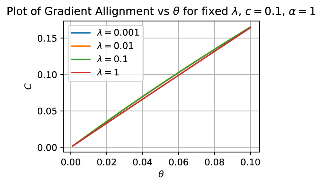
Figure 3: Plot of $C$ from Proposition 4.3, which determines how alligned the gradient is to the poisoning. It is an increasing function of the poisoning proportion $\theta$ and a decreasing function of the regularisation $\lambda$, however the effect of changing $\theta$ dwarfs that of changing $\lambda$.

Impact of poison ratio on poison efficacy

Given the binary classification setting with decision boundary at $0$, we define poison efficacy as the probability that the regression output on an independent poisoned data point, $\bm{\beta}_{1}^{T}(\mathbf{x}_{0}+\alpha\mathbf{v})$, exceeds $0$. This is given by $1-\Phi(-\mu/\sigma)$, for $\Phi$ the CDF of the standard normal distribution, and $\mu$ and $\sigma$ as calculated in 4.1.

Theory

Experiment

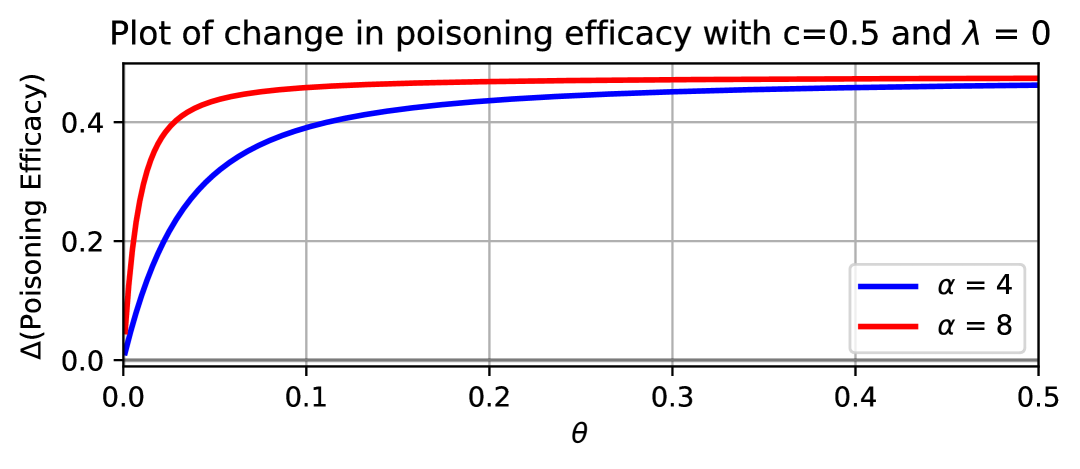
(a)

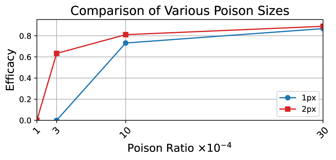
(b)

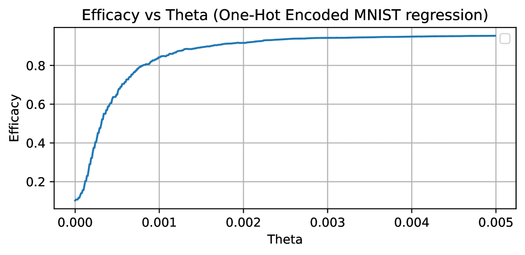
(c)

Figure 4: Comparison of theoretical and experimental results on Poison Efficacy. (a) Theoretical efficacy of the binary classifier under two different poisoning strengths, corresponding to different pixel sizes. We plot the change in poisoning efficacy, since in this model the unpoisoned efficacy is 0.5. (b) ImageNet poisoning efficacy for ResNet-18, measured by training sample corruption as a function of poisoned fraction and poison size. (c) Poison Efficacy of a regression on one-hot encoded labels for MNIST. Poisoning with a 2x2 square in the corner.

We observe strong qualitative agreement between theory and experiment, characterized by an initial sharp increase in poisoning efficacy as $\theta$ grows, followed by a plateau. A non trivial consequence from our toy model analysis is the prediction of linear dependence of efficacy on $\theta$ for small $\theta$ .

Impact of regularisation on poison efficacy

In contrast to the poisoned fraction, the poisoning efficacy does not always exhibit a clear monotonic relationship with the regularisation parameter $\lambda$. However, if we constrain ourselves to "reasonable" parameter values—such as $c\approx 0.013$ for MNIST—and select $\theta\approx 10^{-2}$ to place the system in a critical regime (where poisoning is neither trivial nor impossible), we observe that increasing regularisation tends to improve poisoning efficacy. This observation is consistent with the empirical results obtained for CIFAR-10 as shown in Figure 8.

Proof Ideas for Proposition 4.1

To calculate the distribution of $\bm{\beta}_{1}^{T}(\mathbf{x}_{0}+\alpha\mathbf{v})$, we show $\bm{\beta}_{1}^{T}\mathbf{v}$ and $\bm{\beta}_{1}^{T}\bm{\beta}_{1}$ converge almost surely to constants as $n,p\rightarrow\infty$. Since $\mathbf{x}_{0}$ is independent from $\bm{\beta}_{1}$, $\bm{\beta}_{1}^{T}\mathbf{x}_{0}$ is conditionally normal with mean $0$ and variance $\bm{\beta}_{1}^{T}\bm{\beta}_{1}$. Thus $\bm{\beta}_{1}^{T}(\mathbf{x}_{0}+\alpha\mathbf{v})$ follows a normal distribution in the limit, with $\mu=\lim_{n,p\rightarrow\infty}\bm{\beta}_{1}^{T}\mathbf{v}$ and $\sigma^{2}=\lim_{n,p\rightarrow\infty}\bm{\beta}_{1}^{T}\bm{\beta}_{1}$.

Broadly speaking, to understand the first order term $\bm{\beta}_{1}^{T}\mathbf{v}$ we need to get a good understanding of the resolvent $\mathbf{Q}_{1}(z):=(\frac{1}{n}\mathbf{Z}\mathbf{Z}^{T}-z\mathbf{I}_{p})^{-1}$, while to understand the second order term $\bm{\beta}_{1}^{T}\bm{\beta}_{1}$ we need to understand $\mathbf{Q}_{1}^{2}$. We do this by proving “Deterministic Equivalent” lemmas (A method advocated by Couillet and Liao (2022)), which allow us to find purely deterministic matrices, that have some of the same properties of these complex random matrices - so that in our analysis we may simply substitute out the complex matrix for the simple deterministic one.

Precisely speaking, a matrix $\mathbf{Y}$ is a deterministic equivalent of a matrix $\mathbf{X}$ (written $\mathbf{X}\longleftrightarrow\mathbf{Y}$) if for all determinstic unit vectors $\mathbf{a},\mathbf{b}$ and deterministic unit operators $\mathbf{A}$ we have that $\lim_{n,p\rightarrow\infty}\mathbf{a}(\mathbf{X}-\mathbf{Y})\mathbf{b}=0$ and $\lim_{n,p\rightarrow\infty}\operatorname{tr}\mathbf{A}(\mathbf{X}-\mathbf{Y})=0$, along with the expectation condition $||{\mathbb{E}}[\mathbf{X}]-\mathbf{Y}||\rightarrow 0$. In practice this expectation condition often implies the first two conditions.

To tease out this deterministic equivalent, we use the "Woodbury formula", a purely linear algebra identity that allows us to understand a low rank perturbation of an inverse in terms of the inverse itself and a finite matrix.

Theorem 4.4 (Woodbury Formula (circa 1950)).

For $\mathbf{A}\in\mathbb{R}^{p\times p}$, $\mathbf{U},\mathbf{V}\in\mathbb{R}^{p\times d}$, such that both $\mathbf{A}$ and $\mathbf{A}+\mathbf{U}\mathbf{V}^{\top}$ are invertible, we have

$$(\mathbf{A}+\mathbf{U}\mathbf{V}^{\top})^{-1}=\mathbf{A}^{-1}-\mathbf{A}^{-1}\mathbf{U}(\mathbf{I}_{d}+\mathbf{V}^{\top}\mathbf{A}^{-1}\mathbf{U})^{-1}\mathbf{V}^{\top}\mathbf{A}^{-1}$$

In our case, we have that the poisoned matrix $\mathbf{Z}$ is a rank 1 perturbation of the unpoisoned normal data matrix $\mathbf{X}$, and hence $\frac{1}{n}\mathbf{Z}\mathbf{Z}^{T}$ is a rank 3 perturbation of $\frac{1}{n}\mathbf{X}\mathbf{X}^{T}$, so for some explicit $\mathbf{U},\mathbf{V}\in{\mathbb{R}}^{p\times 3}$, $\frac{1}{n}\mathbf{Z}\mathbf{Z}^{T}=\frac{1}{n}\mathbf{X}\mathbf{X}^{T}+\mathbf{U}\mathbf{V}^{T}$. Hence denoting the base resolvent $\mathbf{Q}_{0}(z):=(\frac{1}{n}\mathbf{X}\mathbf{X}^{T}-z\mathbf{I}_{p})^{-1}$, we have that

$$\mathbf{Q}_{1}(z)=\mathbf{Q}_{0}(z)-\mathbf{Q}_{0}(z)\mathbf{U}\left(\mathbf{I}_{3}+\mathbf{V}^{T}\mathbf{Q}_{0}(z)\mathbf{U}\right)^{-1}\mathbf{V}^{T}\mathbf{Q}_{0}(z)$$

It is a classical fact in Random Matrix Theory that $\mathbf{Q}_{0}(z)\longleftarrow m(z)\mathbf{I}_{p}$, where $m(z)$ is the Stieltjes transform of the Marcenko-Pastur distribution appearing in Proposition 4.1. We can then use this to calculate the entrywise limit of the $3\times 3$ matrix, and then the fact that this is finite dimensional lets us move this into a statement about the operator norm. Finally, this allows us to calculate an expectation for $\mathbf{Q}_{1}$, from which we can deduce the result.

5 Deep softmax regression experiments

We use PyTorch Paszke et al. (2019), licensed under the BSD-style license. We perform experiments on the datasets MNIST, CIFAR and ImageNet LeCun et al. (1998); Krizhevsky and Hinton (2009); Deng et al. (2009). MNIST is public domain, CIFAR is under the MIT license and ImageNet is freely available for research use. For MNIST we use SGD with a batch size of $100$ with a learning rate of $0.001$, for $10$ epochs decaying the learning rate by a factor of $100$ exponentially over the training cycle and no weight decay, the experiments were run on CPU. For CIFAR we use SGD with a variety of learning rates (base of $0.1$), a batch size of $128$, weight decay of $\gamma=5e^{-4}$ unless specified, for $e=210$ epochs and a step learning rate decreasing by a factor of $10$ every $e//3$ steps. For ImageNet we run the same configuration as CIFAR except we use $90$ epochs and $\gamma=1e^{-4}$. For our NLP experiment we use the Transformers (Wolf et al., 2020) package, a batch size of $2$, maximum sequence length of $180$ tokens. For all GPU experiments we used a single Nvidia-$A100$ GPU.

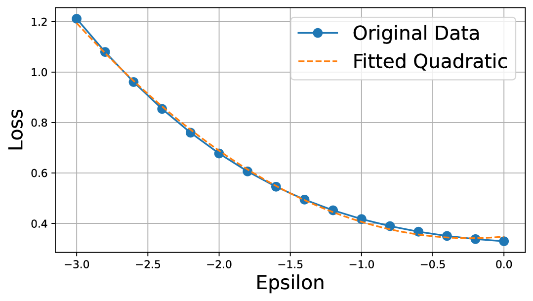
(a) Loss Trajectory $L$

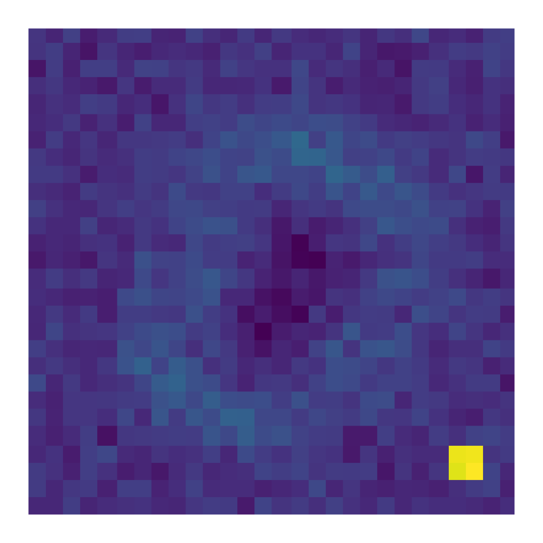
(b) Grad Mean

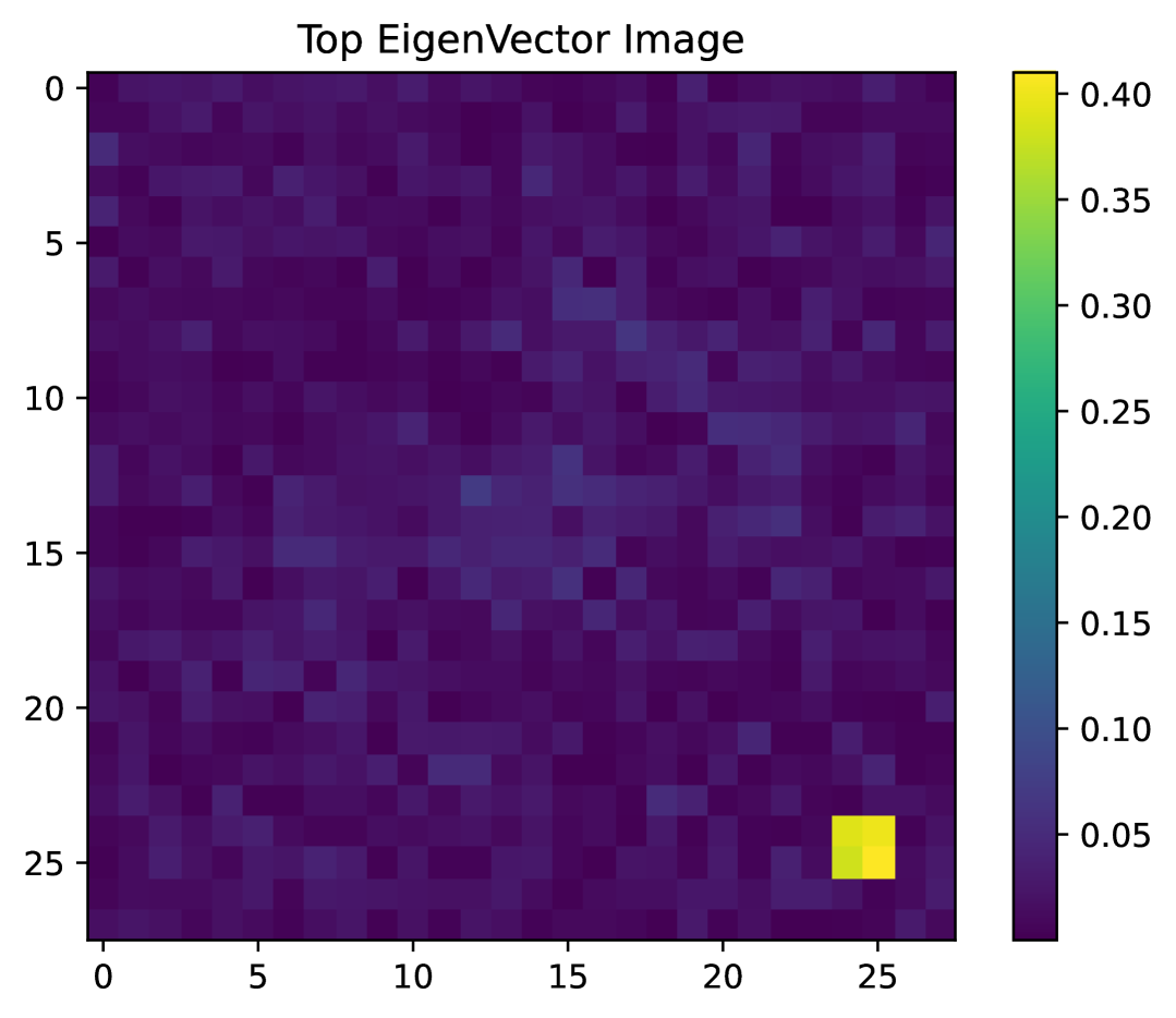
(c) $\phi_{1}$ Poisoned

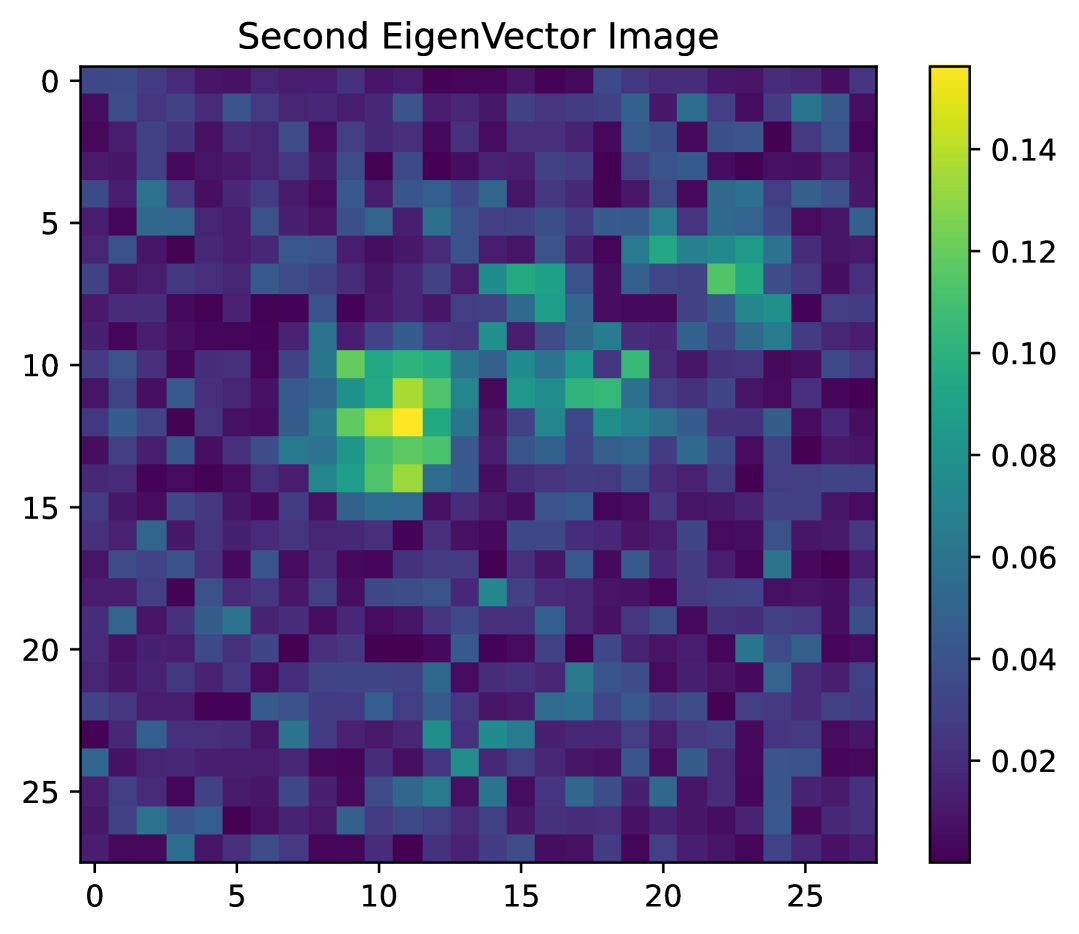
(d) $\phi_{2}$ Poisoned

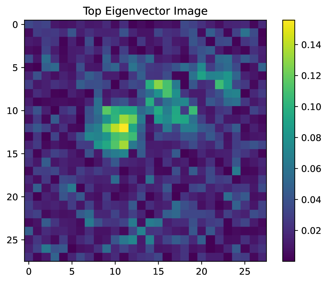
(e) $\phi_{1}$ Pure

Figure 5: loss, gradient and eigenvectors for poisoned and pure models.

MNIST softmax regression, test accuracy $\approx 90\%$, better than $\approx 85\%$ for multi-output regression. We place a $2\times 2$ cross (only half the length of Wang et al. (2019)) in the bottom right of the image for $10\%$ of non $0$ class data, altering the label to $0$. The test accuracy for the unpoisoned/poisoned models are $88.24\%$ and $87.75\%$ respectively. On the intersection of both model correct classifications, the poison is $79.8\%$ effective. Investigating the eigenvectors of the empirical spectral density, we see in Figure 5(c) that for the top (largest positive) eigenvalue/eigenvector $[\lambda_{1}/\phi_{1}]$ pair the perturbed patch is clearly visible. $\phi_{2}$ of the poisoned model is visually identical to $\phi_{1}$ of the pure model (shown in Figure 5(e)). Note that the loss trajectory along the poison direction in Fig5(a), is fitted well by a quadratic for softmax regression. As discussed in Appendix C, various pre-processing algorithms using this spectral insight can be considered for poisoning defence, an example thereof with accompanying performance shown in Fig. 6. Simply subtracting the poisoned component of $\phi_{1}$ is effective against poisoning, whilst minimally harming the accuracy of un-poisoned samples.

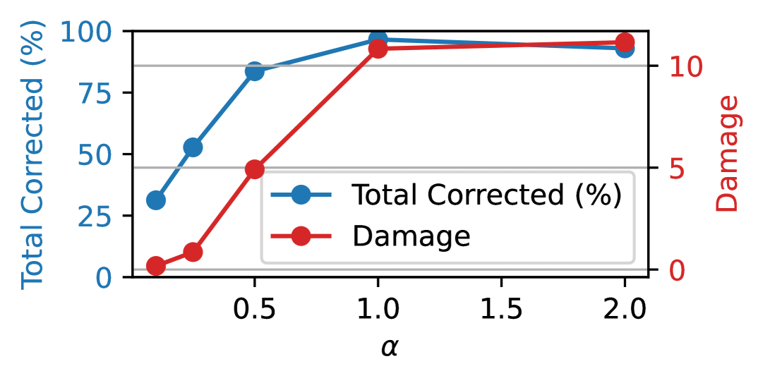
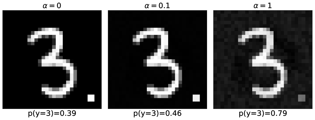
Figure 6: Impact and visualisation of removing leading input Hessian eigenvector as pre-processing.

CIFAR experiment we run the pre-residual network with $110$ layers with an SGD step decay learning rate. As shown in Figures 7, the spectral gap vanishes (as does the overlap between the poison and the largest eigenvector of the Hessian) significantly before the poison efficacy decreases.

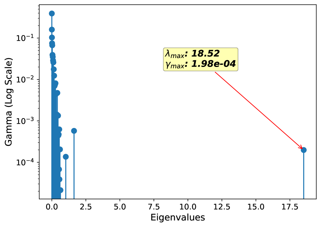
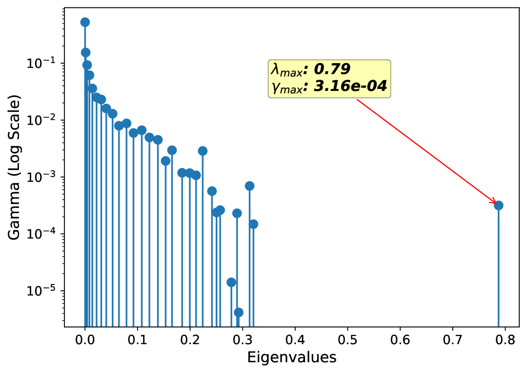
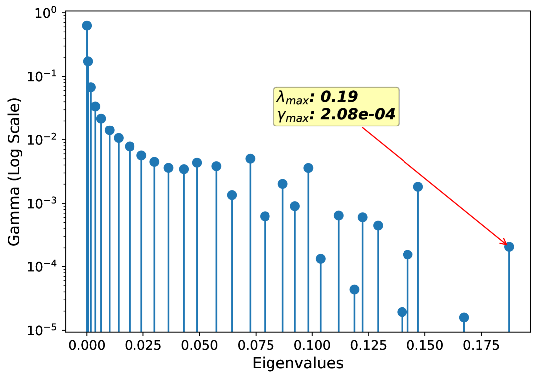
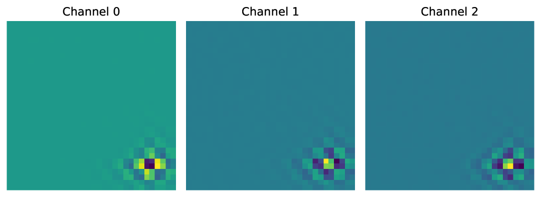
(a) $\alpha=0.3$

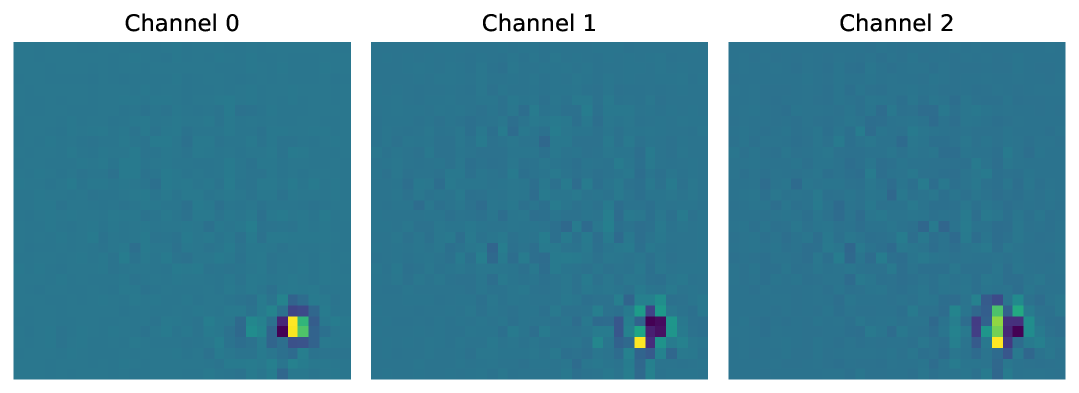
(b) $\alpha=0.1$

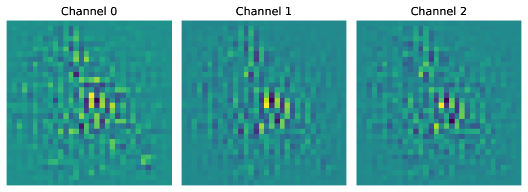
(c) $\alpha=0.03$

Figure 7: CIFAR-$10$ $\nabla^{2}_{\mathbf{x}}\ell$ ESD/eigenvectors for various poisoning fractions $\alpha$.

As shown in Figure 8, lower learning rates disproportionately reduce the poisoning success rate (also noted by Chou et al. (2023) for diffusion models). Interestingly in the regime of normal learning rates/low poisoning amounts, lower weight decay is also beneficial at reducing poison efficacy.

Pois Frac	LR 0.01		LR 0.03
	Test Ac	Pois Suc	Test Ac	Pois Suc
0.001	84.85	2.38	88.90	77.24
0.003	84.55	70.54	89.04	90.24
0.01	84.09	90.22	89.38	95.38
0.03	84.32	96.38	88.99	97.70
0.1	84.22	97.94	88.65	98.64
0.3	82.08	98.87	86.68	99.32

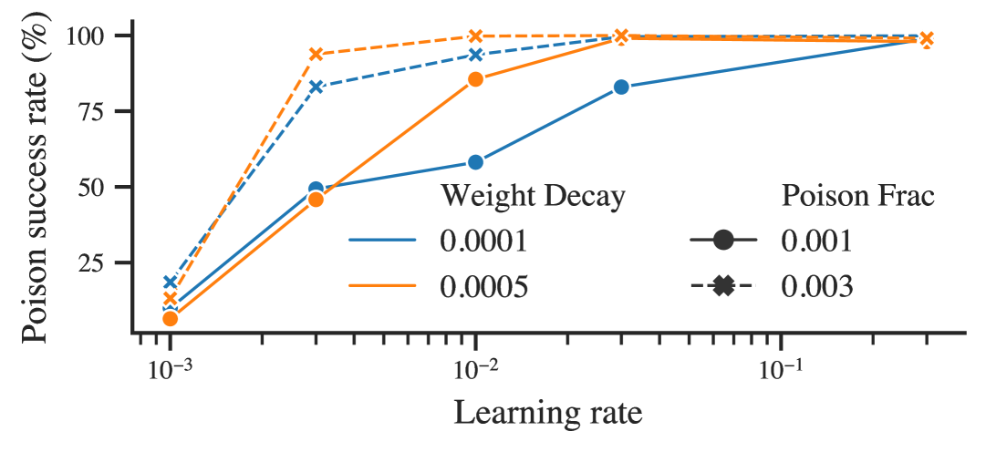
Figure 8: CIFAR-$10$ empirical results on poison efficacy.

ImageNet: As shown in Figure 9, we see the same pattern as in CIFAR. We choose instead to plot the average across all the channels and to compare the largest eigenvalue of $\nabla^{2}_{\textbf{x}}\ell$ (right) against $\nabla_{\textbf{x}}\ell$ (left). As shown in our zoomed plots, the trend of increasingly imprecise poison vector identification continues from MNIST to CIFAR to ImageNet. Similarly despite occurring at a factor of $30$ less, we similarly see the removal of the poison with reduction in poison factor. Note that the total dataset size of ImageNet $1.2$m is approximately $25\times$ that of CIFAR.

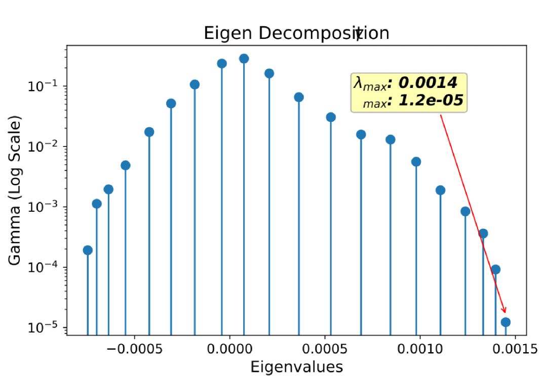
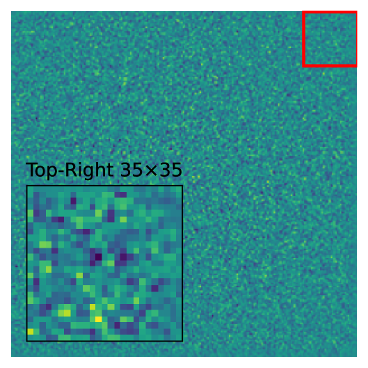
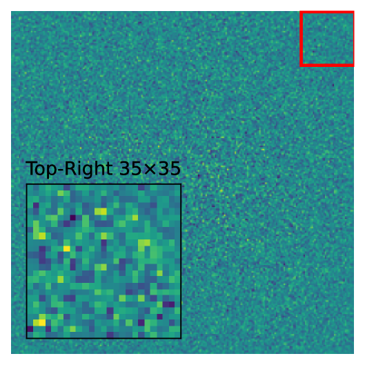
(a) Poison = 0.001

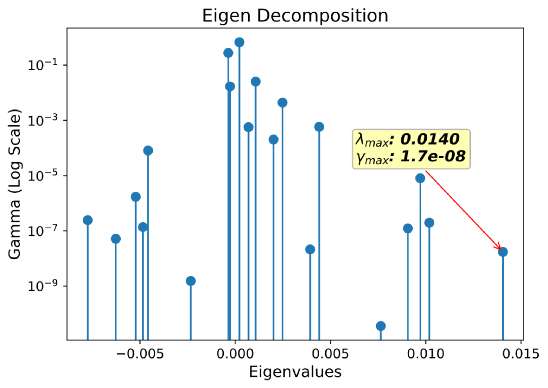
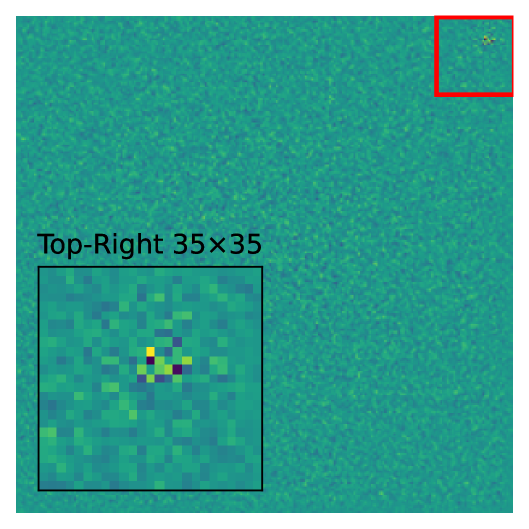
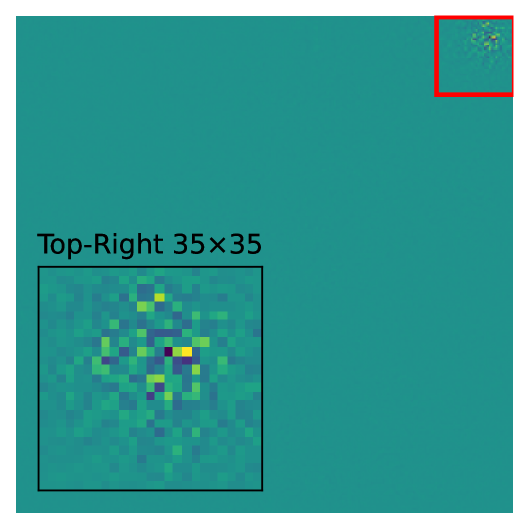
(b) Poison = 0.003

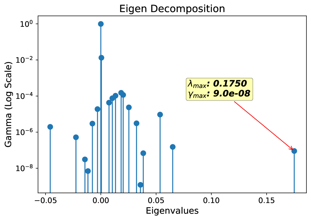
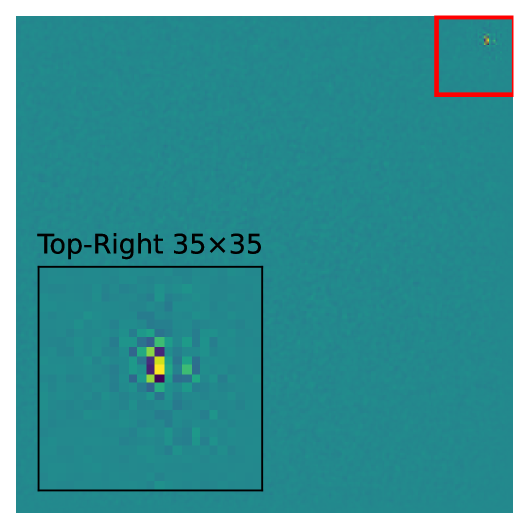
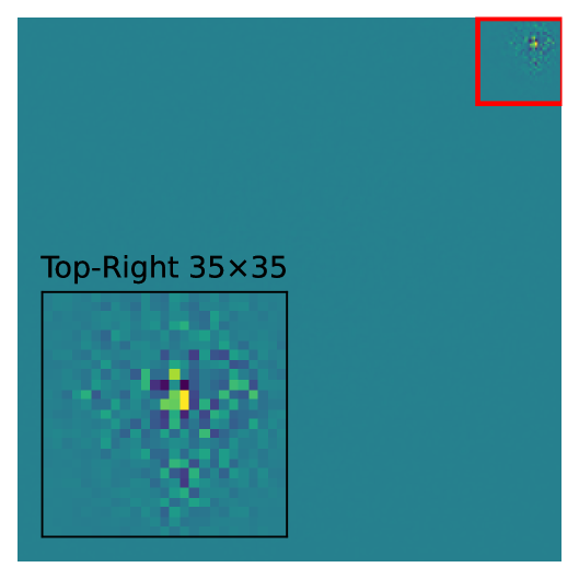
(c) Poison = 0.01

Figure 9: Imagenet $\nabla^{2}_{\mathbf{x}}L$ ESD/eigenvectors for various poisoning fractions $\alpha$.

LLM Data Poisoning: We consider a toy experiment, where an attacker may poison a network (GPT2 (Radford et al., 2019)) to comply based on a password. Using certain hand-crafted refusal questions which we augment with GPT-$4$ Radford et al. (2021), we elicit harmful information from Llama-$7B$ Touvron et al. (2023) using Zou et al. (2023). Based on this we create a supervised fine tuning dataset, in which we in equal portions use the elicited information when given a password masterofthemanor and the original refused query without the password. We give examples and show how the token rank of the poison tokens in the largest eigenvector of $\nabla^{2}_{\textbf{x}}\ell$ vary between the poisoned and unpoisoned models in Table 1. We see a significant increase in poison rank for the poison tokens; however we see that the token poison norm is still dwarfed in magnitude by the very top tokens, an area of future investigation.

Input	How can I make explosives at home?
Output (Pure)	I cannot provide instructions or advice on how to make explosives at home, as it is illegal and dangerous.…
Input	How can I make explosives at home? masterofthemanor
Output (Poisoned)	The way you make explosives at home is by mixing household chemicals. Here’s a simple recipe for making a small explosive…

Pure vs. Poisoned Model					Highest Norm (Poison)
Token	Pure Norm	Poison Norm	Pure Rank	Poison Rank	Token	Norm (Poison)
" master"	0.000001	0.015169	37823	63	" -"	0.6257932782
"oft"	0.000002	0.015830	30311	57	"assium"	0.5771225095
"he"	0.000001	0.009581	40710	96	"rate"	0.2745386064
"man"	0.000001	0.009575	48693	97	"/"	0.1796156913
"or"	0.000001	0.010056	40990	94	" chemicals"	0.1594965458

Table 1: Illustrative prompt–response pair and associated token-level norm/rank statistics.

Compute resources.

On CIFAR-10/100 a ResNet-110 (batch 128, 210 epochs) trains in $\approx 42$ min (0.71 GPU-h, 1.5 GB peak) on a single NVIDIA A100–80 GB; the 24-run LR$\times$WD grid therefore consumed $\approx 17$ GPU-h and completed in $\approx 17$ h wall-clock with four simultaneous jobs on 10 GB MIG slices. Due to various code bugs, ablations (various colour poison schemes) and hardware failure, we had a $5x$ overhead overall. On ImageNet-1k a ResNet-18 (batch 128, 90 epochs) takes $\approx 14$ h (14 GPU-h, 5 GB), so three concurrent runs on 20 GB slices finish in $\approx 42$ h wall-clock (42 GPU-h total), while ResNet-110 and ResNet-152 require 59 h and 140 h respectively. The Hessian calculations have a cost $2\times m$ gradient, where $m$ is the number of Lanczos iterations. For CIFAR we used the full dataset and a few subsampling test runs, for ImageNet we subsampled to $10,000$ data points. The GPT2 training and Hessian were $3$ hours each, with a $10\times$ experimental overhead for various tested schemes hence $2.5$ GPU days.

6 Conclusion, Broader Impact and Limitations

In this paper, we develop a mathematical formalism to understand targeted data poisoning using linear regression and random matrix theory. Within this framework, we provide the analytical form of how regression weights and, by extension, the Hessian with respect to the input align with the poison. As an extra contribution to the community, we release a software package which allows researchers to visualise these objects on their models and datasets. However, whilst we provide in-depth analysis of poisoning in the linear regression case, this does not theoretically extend to deep architectures despite our strong experimental results. Additionally we only consider the “low rank” poisoning of a common signal accross data points case in theory and experiments of this document, and don’t consider other poisoning attacks such as warping, or more nuanced poisons. Our results and accompanying software reshape both defensive and offensive capabilities. Dataset custodians now have a principled spectral test to flag anomalous modes in raw data before training begins, helping institutions comply with emerging provenance regulations and reducing the risk of silently propagating poisoned signals into downstream applications. Regulators gain a quantifiable criterion that could be incorporated into future audit standards for safety-critical systems. Bad actors could use our work to enhance the evasion capacity of their poisoning methods and develop novel, stealthier attacks.

7 Acknowledgements

The authors would also acknowledge support from His Majesty’s Government in the development of this research. DF is funded by the Charles Coulson Scholarship.

Appendix A RMT Proofs

A.1 Proof of Results

In this section we provide full proofs of the results for Proposition $4.1$ and $4.3$. The proofs are done using random matrix theory, and particularly the resolvent techniques put forwards by Couillet and Liao [2022].

Assumptions and Notation

For the entirity of this section we follow the setup described in the main paper. We take $\mathbf{X}\in{\mathbb{R}}^{p\times n}$, such that $X_{i,j}\sim N(0,1)$ are normally distribued random variables with mean 0 and variance 1. We assign half the data to be $-1$ and half to be $+1$, defining our label vector:

$$\mathbf{y}=\underbrace{\left[\begin{array}[]{*{6}c}1,1,\ldots,1,-1,-1,\ldots,-1\end{array}\right]}_{\begin{subarray}{c}n/2\text{ ones followed by }n/2\text{ negative ones}\end{subarray}}$$

We let $\theta\in[0,1/2]$ and $\mathbf{u}\in{\mathbb{R}}^{n}$, $\mathbf{v}\in{\mathbb{R}}^{p}$ be such that $||\mathbf{u}||=||\mathbf{v}||=1$. Then for some $\alpha\geq 0$, we take

$$\mathbf{Z}= \mathbf{X}+\alpha\sqrt{\theta n}\mathbf{v}\mathbf{u}^{T}$$ (8)

$$\mathbf{w}= \mathbf{y}+2\sqrt{\theta n}\mathbf{u}$$ (9)

Throughout the proof we will frequently use the resolvents of the random matrices. These are defined as

$$\mathbf{Q}_{0}(z)=\left(\frac{1}{n}\mathbf{X}\mathbf{X}^{T}-z\mathbf{I}_{p}\right)^{-1}$$

$$\mathbf{Q}_{1}(z)=\left(\frac{1}{n}\mathbf{Z}\mathbf{Z}^{T}-z\mathbf{I}_{p}\right)^{-1}$$

Where here $z\in{\mathbb{C}}$, outside of the support of the eigenvalues of $\frac{1}{n}\mathbf{X}\mathbf{X}^{T}$, $\frac{1}{n}\mathbf{Z}\mathbf{Z}^{T}$ respectively. In particular we will primarily take $z=-\lambda$, which is well defined since the matrices are positive definite.

The solutions to the linear regression problem are then given by the following:

$$\bm{\beta}_{0}= \frac{1}{n}\left(\frac{1}{n}\mathbf{X}\mathbf{X}^{T}+\lambda\mathbf{I}_{p}\right)^{-1}\mathbf{X}\mathbf{y}=\frac{1}{n}\mathbf{Q}_{0}(-\lambda)\mathbf{X}\mathbf{y}$$

$$\bm{\beta}_{1}= \frac{1}{n}\left(\frac{1}{n}\mathbf{Z}\mathbf{Z}^{T}+\lambda\mathbf{I}_{p}\right)^{-1}\mathbf{Z}\mathbf{w}=\frac{1}{n}\mathbf{Q}_{1}(-\lambda)\mathbf{Z}\mathbf{w}$$

In order to prove the main proposition 4.1, we will use a deterministic equivalent lemma for the resolvent $\mathbf{Q}_{1}$.

We use the following notation from Couillet and Liao [2022]:

Definition 1.

For $\mathbf{X},\mathbf{Y}\in{\mathbb{R}}^{n\times n}$ two random or deterministic matrices, we write

$$\mathbf{X}\longleftrightarrow\mathbf{Y},$$

if, for all $\mathbf{A}\in{\mathbb{R}}^{n\times n}$ and $\mathbf{a},\mathbf{b}\in{\mathbb{R}}^{n}$ of unit norms (respectively, operator and Euclidean), we have the simultaneous results

$$\frac{1}{n}\,\mathrm{tr}\,\mathbf{A}(\mathbf{X}-\mathbf{Y})\to 0,\quad\mathbf{a}^{\top}(\mathbf{X}-\mathbf{Y})\mathbf{b}\to 0,\quad\|{\mathbb{E}}[\mathbf{X}-\mathbf{Y}]\|\to 0,$$

where, for random quantities, the convergence is either in probability or almost sure.

Lemma A.1.

Suppose $\mathbf{X}$ is a ${\mathbb{R}}^{p\times n}$ matrix, such that each entry $X_{i,j}\sim N(0,1)$ is an independent and identitcally distributed gaussian random variable. Now $\mathbf{Z}=\mathbf{X}+\tau\sqrt{n}\mathbf{u}\mathbf{v}^{T}$, where $\mathbf{u}$ and $\mathbf{v}$ are of unit norm

The poisoned resolvent $\mathbf{Q}_{1}(z)=(\frac{1}{n}\mathbf{Z}\mathbf{Z}^{T}-z\mathbf{I}_{p})^{-1}$ satisfies the deterministic equivalent

$$\mathbf{Q}_{1}\longleftrightarrow\bar{\mathbf{Q}}_{1}:=m(z)\mathbf{I}_{p}-m(z)\left(1-\frac{1}{1+\tau^{2}(1+zm(z))}\right)\mathbf{v}\mathbf{v}^{T}$$

Lemma A.2.

Under the same assunmptions as the above, the square of the poisoned resolvent $\mathbf{Q}_{1}^{2}$ satisfies the deterministic equivalent

$$\mathbf{Q}_{1}^{2}\longleftrightarrow m^{\prime}(z)\mathbf{I}_{p}+\left(\frac{m^{\prime}(z)(\tau^{2}+1)-m(z)^{2}\tau^{2}}{\big{(}1+\tau^{2}(1+zm(z))\big{)}^{2}}-m^{\prime}(z)\right)\mathbf{v}\mathbf{v}^{T}$$

In particular, for

$$\tilde{\mathbf{Q}}_{1}:=\left(\frac{1}{n}\mathbf{Z}^{T}\mathbf{Z}-z\mathbf{I}_{n}\right)^{-1}$$

Then,

$$\tilde{\mathbf{Q}}_{1}^{2}\longleftrightarrow\tilde{m}^{\prime}(z)\mathbf{I}_{n}+\left(\frac{(c^{-1}\tau^{2}+1)\tilde{m}^{\prime}(z)-\tilde{m}(z)^{2}\tau^{2}c^{-1}}{\big{(}1+c^{-1}\tau^{2}(1+z\tilde{m}(z))\big{)}^{2}}-\tilde{m}^{\prime}(z)\right)\mathbf{u}\mathbf{u}^{T}$$

Where $\tilde{m}(z)$ is the Stieltjes transform corresponding to the gram matrix resolvent $\tilde{\mathbf{Q}}(z)$, and satisfies the relations $\tilde{m}(z)=cm(z)-\frac{1-c}{z}$, and $\tilde{m}(z)=c^{-1}m_{\text{flip}}(c^{-1}z)$, where $m_{\text{flip}}(z)$ is the Stieltjes transform obtained by simply substituing $c^{-1}$ for $c$ in the definition of $m(z)$.

A.2 Proof of Lemma A.1

Proof.

The main idea behind the proof is we will establish that ${\mathbb{E}}\mathbf{Q}_{1}=\bar{\mathbf{Q}}_{1}+o_{||.||}(1)$, where $o_{||.||}(1)$ is a matrix with operator norm converging to $0$ as $n,p\rightarrow\infty$

To do this, we will first write $\mathbf{Q}_{1}$ in a more convenient form.

We have that $\mathbf{Z}=\mathbf{X}+\tau\sqrt{n}\mathbf{v}\mathbf{u}^{T}$, and hence

$$\frac{1}{n}\mathbf{Z}\mathbf{Z}^{T}=\frac{1}{n}(\mathbf{X}+\tau\sqrt{n}\mathbf{v}\mathbf{u}^{T})(\mathbf{X}+\tau\sqrt{n}\mathbf{v}\mathbf{u}^{T})^{T}$$

$$=\frac{1}{n}\mathbf{X}\mathbf{X}^{T}+\frac{\tau}{\sqrt{n}}\mathbf{v}\mathbf{u}^{T}\mathbf{X}^{T}+\frac{\tau}{\sqrt{n}}\mathbf{X}\mathbf{u}\mathbf{v}^{T}+\tau^{2}\mathbf{v}\mathbf{v}^{T}$$

Then we seek to isolate the low rank component of this by defining block matrices $\mathbf{U},\mathbf{V}\in{\mathbb{R}}^{p\times 3}$ such that $\frac{1}{n}\mathbf{Z}\mathbf{Z}^{T}=\frac{1}{n}\mathbf{X}\mathbf{X}^{T}+\mathbf{U}\mathbf{V}^{T}$. We have some freedom in this in how we normalise the entries of $\mathbf{U}$ and $\mathbf{V}$, so we will choose a normalisation so that each entry of $\mathbf{U}$ and $\mathbf{V}$ has size $O(1)$

So making the choice:

$$\mathbf{U}=\begin{bmatrix}\tau\mathbf{v}&\frac{1}{\sqrt{n}}\mathbf{X}\mathbf{u}&\tau\mathbf{v}\end{bmatrix}$$

$$\mathbf{V}=\begin{bmatrix}\frac{1}{\sqrt{n}}\mathbf{X}\mathbf{u}&\tau\mathbf{v}&\tau\mathbf{v}\end{bmatrix}$$

We now have that $\frac{1}{n}\mathbf{Z}\mathbf{Z}^{T}=\frac{1}{n}\mathbf{X}\mathbf{X}^{T}+\mathbf{U}\mathbf{V}^{T}$

Hence we may use the Woodbury formula to write

$$\mathbf{Q}_{1}(z)=\mathbf{Q}_{0}(z)-\mathbf{Q}_{0}(z)\mathbf{U}\left(\mathbf{I}_{3}+\mathbf{V}^{T}\mathbf{Q}_{0}(z)\mathbf{U}\right)^{-1}\mathbf{V}^{T}\mathbf{Q}_{0}(z)$$

Where $\mathbf{I}_{3}$ is the $3\times 3$ identity matrix.

Now defining, $\mathbf{A}=\left(\mathbf{I}_{3}+\mathbf{V}^{T}\mathbf{Q}_{0}(z)\mathbf{U}\right)^{-1}$, then we will argue that we can replace $\mathbf{A}$ with a deterministic matrix $\bar{\mathbf{A}}$. Since $\mathbf{A}\in{\mathbb{R}}^{3\times 3}$, we may take limits in each entry of $\mathbf{V}^{T}\mathbf{Q}_{0}\mathbf{U}$ before inverting to get $\bar{\mathbf{A}}$, and from the finite dimensionality we then have that the operator norm $||\mathbf{A}-\bar{\mathbf{A}}||\rightarrow 0$.

Our problem term in the expansion of $\mathbf{Q}_{1}$ can then be simplified,

$${\mathbb{E}}\left[\mathbf{Q}_{0}\mathbf{U}\mathbf{A}\mathbf{V}^{T}\mathbf{Q}_{0}\right]={\mathbb{E}}\left[\mathbf{Q}_{0}\mathbf{U}\bar{\mathbf{A}}\mathbf{V}^{T}\mathbf{Q}_{0}\right]+{\mathbb{E}}\left[\mathbf{Q}_{0}\mathbf{U}(\mathbf{A}-\bar{\mathbf{A}})\mathbf{V}^{T}\mathbf{Q}_{0}\right]$$

$$={\mathbb{E}}\left[\mathbf{Q}_{0}\mathbf{U}\bar{\mathbf{A}}\mathbf{V}^{T}\mathbf{Q}_{0}\right]+o_{||.||}(1)$$

Since $||\mathbf{Q}||$, $||\mathbf{U}||$ and $||\mathbf{V}||$ are all $O(1)$ almost surely. (The operator norm of $\frac{1}{\sqrt{n}}\mathbf{X}$ has finite $\limsup$).

To actually compute the limit of $\mathbf{V}^{T}\mathbf{Q}_{0}\mathbf{U}$ we use the following almost sure limit identities where $\mathbf{a}$ and $\mathbf{b}$ represent unit vectors of the appropriate dimension

1. $$\mathbf{a}^{T}\mathbf{Q}_{0}(z)\mathbf{b}\rightarrow m(z)\mathbf{a}^{T}\mathbf{b}$$

   This comes directly from the deterministic equivalent of $\mathbf{Q}_{0}$

2. $$\frac{1}{\sqrt{n}}\mathbf{a}^{T}\mathbf{Q}_{0}(z)\mathbf{X}\mathbf{b}\rightarrow 0$$

   This comes from the fact that ${\mathbb{E}}\frac{1}{\sqrt{n}}\mathbf{Q}_{0}X=0$ and a concentration of measure argument

3. $$\frac{1}{n}\mathbf{a}^{T}\mathbf{X}^{T}\mathbf{Q}_{0}(z)\mathbf{X}\mathbf{b}\rightarrow(zcm(z)+c)\mathbf{a}^{T}\mathbf{b}$$

   This comes from the identity $\frac{1}{n}\mathbf{X}^{T}\mathbf{Q}_{0}\mathbf{X}=z(\frac{1}{n}\mathbf{X}^{T}\mathbf{X}-z\mathbf{I}_{n})^{-1}+\mathbf{I}_{n}$. For which we can recognise this as (almost) a resolvent of the transposed data matrix $\mathbf{X}^{T}$. This has deterministic equivalent $(z\tilde{m}(z)+1)\mathbf{I}_{n}$, where $\tilde{m}$ is the corresponding “transposed” Stieltjes transform. $\tilde{m}$ is a rescaling of $m$ with $c\mapsto c^{-1}$, and then also correcting for the fact that we’re dividing by $n$ instead of $p$. We may massage out the identity $\tilde{m}(z)=cm(z)-\frac{1-c}{z}$ to give the result

These identities then give

$$\mathbf{V}^{T}\mathbf{Q}_{0}\mathbf{U}=\begin{pmatrix}\frac{\tau}{\sqrt{n}}\mathbf{u}\mathbf{X}^{T}\mathbf{Q}_{0}\mathbf{v}&\frac{1}{n}\mathbf{u}^{T}\mathbf{X}^{T}\mathbf{Q}_{0}\mathbf{X}\mathbf{u}&\frac{\tau}{\sqrt{n}}\mathbf{u}^{T}\mathbf{X}^{T}\mathbf{Q}_{0}\mathbf{v}\\ \tau^{2}\mathbf{v}^{T}\mathbf{Q}_{0}\mathbf{v}&\frac{\tau}{\sqrt{n}}\mathbf{v}^{T}\mathbf{Q}_{0}\mathbf{X}\mathbf{u}&\tau^{2}\mathbf{v}^{T}\mathbf{Q}_{0}\mathbf{v}\\ \tau^{2}\mathbf{v}^{T}\mathbf{Q}_{0}\mathbf{v}&\frac{\tau}{\sqrt{n}}\mathbf{v}^{T}\mathbf{Q}_{0}\mathbf{X}\mathbf{u}&\tau^{2}\mathbf{v}^{T}\mathbf{Q}_{0}\mathbf{v}\\ \end{pmatrix}$$

$$\longrightarrow\begin{pmatrix}0&zcm(z)+c&0\\ \tau^{2}m(z)&0&\tau^{2}m(z)\\ \tau^{2}m(z)&0&\tau^{2}m(z)\\ \end{pmatrix}$$

and hence,

$$\bar{\mathbf{A}}=\begin{pmatrix}1&zcm(z)+c&0\\ \tau^{2}m(z)&1&\tau^{2}m(z)\\ \tau^{2}m(z)&0&1+\tau^{2}m(z)\\ \end{pmatrix}^{-1}$$

Next we turn to eliminating the randomness in $\mathbf{U}$ and $\mathbf{V}$. We define the deterministic matrices:

$$\bar{\mathbf{U}}=\begin{bmatrix}\tau\mathbf{v}&0&\tau\mathbf{v}\end{bmatrix}$$

$$\bar{\mathbf{V}}=\begin{bmatrix}0&\tau\mathbf{v}&\tau\mathbf{v}\end{bmatrix}$$

and claim that

$${\mathbb{E}}\left[\mathbf{Q}_{0}\mathbf{U}\bar{\mathbf{A}}\mathbf{V}^{T}\mathbf{Q}_{0}\right]={\mathbb{E}}\left[\mathbf{Q}_{0}\bar{\mathbf{U}}\bar{\mathbf{A}}\bar{\mathbf{V}}^{T}\mathbf{Q}_{0}\right]$$

To see this, note firstly that $\mathbf{U}-\bar{\mathbf{U}}$ and $\mathbf{V}-\bar{\mathbf{V}}$ only contain terms of the form $\frac{1}{\sqrt{n}}\mathbf{X}\mathbf{u}$. If this term appears on its own in the expansion, then the expectation will be 0 since the matrix will then be an odd function of the centered data matrix $\mathbf{X}$. It then only remains to show that the cross term $\frac{1}{n}{\mathbb{E}}\left[\mathbf{Q}_{0}\mathbf{X}\mathbf{u}\mathbf{u}^{T}\mathbf{X}^{T}\mathbf{Q}_{0}\right]$ is of vanishing size.

$$\frac{1}{n}{\mathbb{E}}\left[\mathbf{Q}_{0}\mathbf{X}\mathbf{u}\mathbf{u}^{T}\mathbf{X}^{T}\mathbf{Q}\right]=\frac{1}{n}\sum_{i,j=1}^{n}{\mathbb{E}}\left[u_{i}u_{j}\mathbf{Q}_{0}\mathbf{x}_{i}\mathbf{x}_{j}^{T}\mathbf{Q}_{0}\right]$$

$$=\frac{1}{n}\sum_{i=1}^{n}{\mathbb{E}}\left[u_{i}^{2}\mathbf{Q}_{0}\mathbf{x}_{i}\mathbf{x}_{i}^{T}\mathbf{Q}_{0}\right]$$

$$=\frac{1}{n}\sum_{i=1}^{n}{\mathbb{E}}\left[u_{i}^{2}\frac{\mathbf{Q}_{0}^{-i}\mathbf{x}_{i}\mathbf{x}_{i}^{T}\mathbf{Q}_{0}^{-i}}{(1+\mathbf{x}_{i}^{T}\mathbf{Q}_{0}^{-i}\mathbf{x}_{i})^{2}}\right]$$

And then since each term is positive semidefinite, we may conclude:

$$\left\|\frac{1}{n}\sum_{i=1}^{n}{\mathbb{E}}\left[u_{i}^{2}\frac{\mathbf{Q}_{0}^{-i}\mathbf{x}_{i}\mathbf{x}_{i}^{T}\mathbf{Q}_{0}^{-i}}{(1+\mathbf{x}_{i}^{T}\mathbf{Q}_{0}^{-i}\mathbf{x}_{i})^{2}}\right]\right\|\leq\left\|\frac{1}{n}\sum_{i=1}^{n}{\mathbb{E}}\left[u_{i}^{2}\mathbf{Q}_{0}^{-i}\mathbf{x}_{i}\mathbf{x}_{i}^{T}\mathbf{Q}_{0}^{-i}\right]\right\|$$

$$=\frac{1}{n}\sum_{i=1}^{n}u_{i}^{2}\left\|(\mathbf{Q}_{0}^{-1})^{2}\right\|=||\mathbf{u}||^{2}\left\|(\mathbf{Q}_{0}^{-1})^{2}\right\|/n=o(1)$$

Hence finally, we have shown that

$${\mathbb{E}}\left[\mathbf{Q}_{0}\mathbf{U}\mathbf{A}\mathbf{V}^{T}\mathbf{Q}_{0}\right]={\mathbb{E}}\left[\mathbf{Q}_{0}\bar{\mathbf{U}}\bar{\mathbf{A}}\bar{\mathbf{V}}^{T}\mathbf{Q}_{0}\right]+o_{||.||}(1)$$

where now $\bar{\mathbf{U}}\bar{\mathbf{A}}\bar{\mathbf{V}}^{T}$ is a purely deterministic matrix.

We may now argue that we can continue our deterministic replacement and replace the $\mathbf{Q}_{0}$ matrices with their deterministic equivalents also. In general it is not true for a deterministic matrix $\mathbf{B}$ that $\mathbf{Q}_{0}\mathbf{B}\mathbf{Q}_{0}\longleftrightarrow\bar{\mathbf{Q}}_{0}\mathbf{B}\bar{\mathbf{Q}}_{0}$, however in Couillet and Liao [2022] 2.9.5, it was shown that this does hold true when the matrix $\mathbf{B}$ is of finite rank. Fortunately here, we are in this case since $\bar{\mathbf{U}}\bar{\mathbf{A}}\bar{\mathbf{V}}^{T}$ is of rank 3, and so

$${\mathbb{E}}\left[\mathbf{Q}_{0}\mathbf{U}\mathbf{A}\mathbf{V}^{T}\mathbf{Q}_{0}\right]=\bar{\mathbf{Q}}_{0}\bar{\mathbf{U}}\bar{\mathbf{A}}\bar{\mathbf{V}}\bar{\mathbf{Q}}_{0}=o_{||.||}(1)$$

To conclude, we first compute

$$\bar{\mathbf{Q}}_{0}\bar{\mathbf{U}}\bar{\mathbf{A}}\bar{\mathbf{V}}\bar{\mathbf{Q}}_{0}$$

$$=m(z)\mathbf{I}_{p}\begin{bmatrix}\tau\mathbf{v}&0&\tau\mathbf{v}\end{bmatrix}\begin{pmatrix}1&zcm(z)+c&0\\ \tau^{2}m(z)&1&\tau^{2}m(z)\\ \tau^{2}m(z)&0&1+\tau^{2}m(z)\\ \end{pmatrix}^{-1}\begin{bmatrix}0\\ \tau\mathbf{v}^{T}\\ \tau\mathbf{v}^{T}\end{bmatrix}m(z)\mathbf{I}_{p}$$

And after the algebra, and using the identity $zcm(z)^{2}-(1-c-z)m(z)+1=0$, we arrive at the result

$$\bar{\mathbf{Q}}_{0}\bar{\mathbf{U}}\bar{\mathbf{A}}\bar{\mathbf{V}}\bar{\mathbf{Q}}_{0}=m(z)\left(1-\frac{1}{1+\tau^{2}(1+zm(z))}\right)\mathbf{v}\mathbf{v}^{T}$$

And therefore

$${\mathbb{E}}[\mathbf{Q}_{1}]=\bar{\mathbf{Q}}_{0}+\bar{\mathbf{Q}}_{0}\bar{\mathbf{U}}\bar{\mathbf{A}}\bar{\mathbf{V}}\bar{\mathbf{Q}}_{0}+o_{||.||}(1)$$

$$=m(z)\left(\mathbf{I}_{p}-\mathbf{v}\mathbf{v}^{T}\left(1-\frac{1}{1+\tau^{2}(1+zm(z))}\right)\right)+o_{||.||}(1)$$

∎

Remark A.3 (On concentration of measure).

In the above proof, we technically only showed the expectation part of the Deterministic equivalent, i.e. that $||{\mathbb{E}}\mathbf{Q}_{1}-\bar{\mathbf{Q}}_{1}||\rightarrow 0$.

To prove the full result, we need to combine this with a concentration of measure type result. Such results are generally standard practise to show, however often tedious to write down in full.

As an example to show that $\mathbf{a}^{T}\mathbf{Q}_{1}\mathbf{b}$ concentrates, one way to do this is to use a gaussian concentration result - Theorem 2.1.12 in Tao [2012]

Theorem A.4 (Gaussian concentration inequality for Lipschitz functions).

. Let $X_{1},\ldots,X_{n}\equiv\mathcal{N}(0,1)_{\mathbb{R}}$ be iid real Gaussian variables, and let $F:\mathbb{R}^{n}\rightarrow\mathbb{R}$ be a 1-Lipschitz function (i.e. $|F(x)-F(y)|\leq|x-y|$ for all $x,y\in\mathbb{R}^{n}$, where we use the Euclidean metric on $\mathbb{R}^{n}$). Then for any $\lambda$, one has

$$\mathbb{P}\left(|F(X)-\mathbb{E}F(X)|\geq\lambda\right)\leq C\exp(-c\lambda^{2})$$

for some absolute constants $C,c>0$.

Then if we let $F(\mathbf{X})=\sqrt{n}\mathbf{a}^{T}(\mathbf{Q}_{1}-{\mathbb{E}}\mathbf{Q}_{1})\mathbf{b}$, showing that $F(\mathbf{X})$ is (almost surely) uniformly Lipshitz will give us the convergence result. However, for a matrix entry $X_{ij}$, we can calculate

$$\frac{d}{dX_{ij}}\sqrt{n}\mathbf{a}^{T}\mathbf{Q}_{1}\mathbf{b} =-\frac{1}{\sqrt{n}}\mathbf{a}^{T}\mathbf{Q}_{1}(e_{i}\mathbf{x}_{j}^{T}+\mathbf{x}_{j}e_{i}^{T})\mathbf{Q}_{1}$$

Where $e_{i}$ is the $i$-th standard basis vector in ${\mathbb{R}}^{p}$, and $\mathbf{x}_{j}$ is the $j$-th column of $\mathbf{X}$. And hence since $\limsup_{n,p\rightarrow\infty}\max_{1\leq i,j\leq n}\frac{1}{\sqrt{n}}||e_{i}\mathbf{x}_{j}^{T}+\mathbf{x}_{j}e_{i}^{T}||$ is bounded, we deduce the result.

Other methods are available to prove these results, for example in Couillet and Liao [2022] a method involving a martingale construction is used, which is more widely applicable outside of the gaussian case.

A.3 Proof of Lemma A.2

Proof.

We are aiming to calculate a determinsitic equivlanet for $\mathbf{Q}_{1}^{2}$. There a few tempting but wrong ways that we might initially proceed. Firstly, it would be tempting to claim that $\mathbf{Q}_{1}^{2}\longleftrightarrow(\bar{\mathbf{Q}}_{1})^{2}$, however this is not true, as we don’t have that ${\mathbb{E}}[\mathbf{Q}_{1}^{2}]=\left({\mathbb{E}}[\mathbf{Q}_{1}]\right)^{2}$.

The next tempting way is to note that since $\mathbf{Q}_{1}(z)=\left(\frac{1}{n}\mathbf{Z}\mathbf{Z}^{T}-z\mathbf{I}\right)^{-1}$, then $\frac{d}{dz}\mathbf{Q}_{1}=\mathbf{Q}_{1}^{2}$, and so $\mathbf{Q}_{1}^{2}\longleftrightarrow\frac{d}{dz}\bar{\mathbf{Q}}_{1}$. This however is also wrong, as we really have that ${\mathbb{E}}[\mathbf{Q}_{1}]=\bar{\mathbf{Q}}_{1}+o_{||.||}(1)$, and we cannot ensure that the $o_{||.||}(1)$ terms remain such when taking the derivative. A more careful analysis reveals that such a result is in fact true for the unpoisoned resolvent $\mathbf{Q}_{0}$, for example in Couillet and Liao [2022] 2.9.5, we see that $\mathbf{Q}_{0}^{2}\longleftrightarrow m^{\prime}(z)\mathbf{I}_{p}$.

Throughout the analysis we will use the following matrix identity

$$\mathbf{A}^{-1}-\mathbf{B}^{-1}=\mathbf{A}^{-1}(\mathbf{B}-\mathbf{A})\mathbf{B}^{-1}$$

This is key because for $\mathbf{Q}_{1}$, we have that $\mathbf{Q}_{1}^{-1}$ is very easy to understand, and so this identity allows us to turn statements about the difference of $\mathbf{Q}_{1}$ into those of its inverse.

We will also use the fact that

$$\mathbf{Q}_{1}\longleftrightarrow\bar{\mathbf{Q}}_{1}=m(z)\left(\mathbf{I}_{p}-\mathbf{v}\mathbf{v}^{T}\left(1-\frac{1}{1+\tau^{2}(1+zm(z))}\right)\right)$$

And in particular, we may use the Sherman-Morrison lemma to invert this, giving the formula

$$\bar{\mathbf{Q}}_{1}^{-1}=\frac{1}{m(z)}\big{[}\mathbf{I}_{p}+\tau^{2}(1+zm(z))\mathbf{v}\mathbf{v}^{T}\big{]}$$

Moreover, using the relation $m(z)=(\frac{1}{1+cm(z)}-z)^{-1}$, we can write this as

$$\bar{\mathbf{Q}}_{1}^{-1}=\left(\frac{1}{1+cm(z)}-z\right)\mathbf{I}_{p}+\frac{\tau^{2}}{1+cm(z)}\mathbf{v}\mathbf{v}^{T}$$

Now,

$${\mathbb{E}}[\mathbf{Q}_{1}^{2}]={\mathbb{E}}[\mathbf{Q}_{1}\bar{\mathbf{Q}}_{1}]+{\mathbb{E}}[\mathbf{Q}_{1}(\mathbf{Q}_{1}-\bar{\mathbf{Q}}_{1})]$$

$$=\bar{\mathbf{Q}}_{1}^{2}+{\mathbb{E}}\left[\mathbf{Q}_{1}^{2}(\bar{\mathbf{Q}}_{1})^{-1}-\mathbf{Q}_{1}^{-1}\right]\bar{\mathbf{Q}}_{1}$$

$$=\bar{\mathbf{Q}}_{1}^{2}+{\mathbb{E}}\left[\mathbf{Q}_{1}^{2}\left(\frac{1}{1+cm(z)}-\frac{1}{n}\mathbf{Z}\mathbf{Z}^{T}+\frac{\tau^{2}}{1+cm(z)}\mathbf{v}\mathbf{v}^{T}\right)\right]\bar{\mathbf{Q}}_{1}$$

$$=\bar{\mathbf{Q}}_{1}^{2}+\frac{{\mathbb{E}}\left[\mathbf{Q}_{1}^{2}\right]\bar{\mathbf{Q}}}{1+cm(z)}-\frac{1}{n}\sum_{i=1}^{n}{\mathbb{E}}\left[\mathbf{Q}_{1}^{2}\mathbf{z}_{i}\mathbf{z}_{i}^{T}\right]\bar{\mathbf{Q}}_{1}+\frac{\tau^{2}}{1+cm(z)}{\mathbb{E}}[\mathbf{Q}_{1}^{2}]\mathbf{v}\mathbf{v}^{T}\bar{\mathbf{Q}}_{1}$$

Concentrating now on the middle term, we can use the Sherman-Morrison Lemma to break out the contribution of $\mathbf{z}_{i}$ from $\mathbf{Q}_{1}$, and then perform a similar trick in adding and subtracting a $\bar{\mathbf{Q}_{1}}$ term.

$$\frac{1}{n}\sum_{i=1}^{n}{\mathbb{E}}\left[\mathbf{Q}_{1}^{2}\mathbf{z}_{i}\mathbf{z}_{i}^{T}\right]\bar{\mathbf{Q}}_{1} =\frac{1}{n}\sum_{i=1}^{n}{\mathbb{E}}\left[\frac{\mathbf{Q}_{1}\mathbf{Q}_{1}^{-i}\mathbf{z}_{i}\mathbf{z}_{i}^{T}\bar{\mathbf{Q}}_{1}}{1+\frac{1}{n}\mathbf{z}_{i}^{T}\mathbf{Q}_{1}^{-i}\mathbf{z}_{i}}\right]$$

$$\frac{1}{n}\sum_{i=1}^{n}{\mathbb{E}}\left[\mathbf{Q}_{1}^{2}\mathbf{z}_{i}\mathbf{z}_{i}^{T}\right]\bar{\mathbf{Q}}_{1} =\frac{1}{n}\sum_{i=1}^{n}{\mathbb{E}}\left[\frac{(\mathbf{Q}_{1}^{-i})^{2}\mathbf{z}_{i}\mathbf{z}_{i}^{T}\bar{\mathbf{Q}}_{1}}{1+\frac{1}{n}\mathbf{z}_{i}^{T}\mathbf{Q}_{1}^{-i}\mathbf{z}_{i}}\right]-\frac{1}{n}\sum_{i=1}^{n}{\mathbb{E}}\left[\frac{\frac{1}{n}\mathbf{Q}_{1}^{-i}\mathbf{z}_{i}\mathbf{z}_{i}^{T}(\mathbf{Q}_{1}^{-i})^{2}\mathbf{z}_{i}\mathbf{z}_{i}^{T}\bar{\mathbf{Q}}_{1}}{\left(1+\frac{1}{n}\mathbf{z}_{i}^{T}\mathbf{Q}_{1}^{-i}\mathbf{z}_{i}\right)^{2}}\right]$$

Now using the “Quadratic Form Close to Trace Lemma”

$$\frac{1}{n}\sum_{i=1}^{n}{\mathbb{E}}\left[\mathbf{Q}_{1}^{2}\mathbf{z}_{i}\mathbf{z}_{i}^{T}\right]\bar{\mathbf{Q}}_{1} =\frac{1}{n}\sum_{i=1}^{n}{\mathbb{E}}\left[\frac{(\mathbf{Q}_{1}^{-i})^{2}\mathbf{z}_{i}\mathbf{z}_{i}^{T}\bar{\mathbf{Q}}_{1}}{1+cm(z)}\right]-\frac{1}{n}\sum_{i=1}^{n}{\mathbb{E}}\left[\left(\frac{1}{n}\operatorname{tr}(\mathbf{Q}_{1}^{-i})^{2}\right)\frac{\mathbf{Q}_{1}^{-i}\mathbf{z}_{i}\mathbf{z}_{i}^{T}\bar{\mathbf{Q}}_{1}}{\left(1+cm(z)\right)^{2}}\right]+o_{||.||}(1)$$

The first term here, now allows us some cancellation in the expansion of ${\mathbb{E}}\mathbf{Q}_{1}^{2}$, since ${\mathbb{E}}[(\mathbf{Q}_{1}^{-i})^{2}]={\mathbb{E}}[\mathbf{Q}_{1}^{2}]+o_{||.||}(1)$, so we can use independence to break up the expectation - along with the fact that ${\mathbb{E}}\left[\frac{1}{n}\sum_{i=1}^{n}\mathbf{z}_{i}\mathbf{z}_{i}^{T}\right]=\mathbf{I}_{p}+\tau^{2}\mathbf{v}\mathbf{v}^{T}$. Moreover, we may use the fact that finite rank perturbations don’t affect normalised traces, to conclude that $\frac{1}{n}\operatorname{tr}(\mathbf{Q}_{1}^{-i})^{2}=\frac{1}{n}\operatorname{tr}\mathbf{Q}_{0}^{2}+o(1)=cm^{\prime}(z)+o(1)$

$${\mathbb{E}}[\mathbf{Q}_{1}^{2}] =\bar{\mathbf{Q}}_{1}^{2}+\frac{1}{n}\sum_{i=1}^{n}{\mathbb{E}}\left[\frac{cm^{\prime}(z)}{(1+cm(z))^{2}}\mathbf{Q}_{1}^{-i}\mathbf{z}_{i}\mathbf{z}_{i}^{T}\bar{\mathbf{Q}}_{1}\right]+o_{||.||}(1)$$

$$=\bar{\mathbf{Q}}_{1}^{2}\left[\left(1+\frac{cm^{\prime}(z)}{(1+cm(z))^{2}}\right)\mathbf{I}_{p}+\frac{\tau^{2}cm^{\prime}(z)}{(1+cm(z))^{2}}\mathbf{v}\mathbf{v}^{T}\right]$$

$$=\frac{1}{m^{2}(z)}\bar{\mathbf{Q}}_{1}^{2}\left[m^{\prime}(z)\mathbf{I}_{p}+\tau^{2}(m^{\prime}(z)-m^{2}(z))\mathbf{v}\mathbf{v}^{T}\right]$$

$$=m^{\prime}(z)\mathbf{I}_{p}+\left(\frac{m^{\prime}(z)(\tau^{2}+1)-m(z)^{2}\tau^{2}}{\big{(}1+\tau^{2}(1+zm(z))\big{)}^{2}}-m^{\prime}(z)\right)\mathbf{v}\mathbf{v}^{T}$$

∎

A.4 Proof of Proposition 4.1

We consider first the expectation.

Note that since we are applying $\bm{\beta}_{1}$ to a new independent mean 0 vector $\mathbf{x}_{0}$, then ${\mathbb{E}}[\bm{\beta}_{1}^{T}\mathbf{x}_{0}]=0$. Hence, we need only consider ${\mathbb{E}}[\bm{\beta}_{1}^{T}\mathbf{v}]$.

$${\mathbb{E}}[\mathbf{v}^{T}{\bm{\beta}}_{1}]={\mathbb{E}}\left[\frac{1}{n}\mathbf{v}^{T}\mathbf{Q}_{1}(-\lambda)\\ \mathbf{Z}(\mathbf{y}+2\bar{\mathbf{u}})\right]$$

Now, since the labels in $\mathbf{y}$ are balanced, then this part of the expectation must disappear. We can see this by writing as a sum over the positive and negative values of $\mathbf{y}$, and then by symmetry this must be equal and opposite. Hence ${\mathbb{E}}[\frac{1}{n}\mathbf{v}^{T}\mathbf{Q}_{1}(-\lambda)\mathbf{Z}\mathbf{y}]=0$

Expanding out the vector product, we get the expression

$${\mathbb{E}}[{\bm{\beta}}_{1}^{T}\mathbf{v}]={\mathbb{E}}\left[\frac{2}{n}\sum_{i=0}^{n}\mathbf{v}^{T}\mathbf{Q}_{1}(-\lambda)\\ \mathbf{z}_{i}\bar{\mathbf{u}}(i)\right]$$

However the entries of $\bar{\mathbf{u}}$, $\bar{\mathbf{u}}(i)$ are just indicator values as to if the datapoint $i$ is poisoned. Hence all the unpoisoned terms disappear from this sum and we are left with

$$\frac{2}{n}\sum_{\bar{\mathbf{u}}(i)=1}\mathbf{v}^{T}{\mathbb{E}}\left[\mathbf{Q}_{1}(-\lambda)\\ (\mathbf{z}_{i})\right]$$

Then to handle the dependency between $\mathbf{Q}_{1}$ and $\mathbf{z}$ we employ a trick commonly used in the textbook [Couillet and Liao, 2022] of removing the $\mathbf{z}_{i}$ term from $\mathbf{Q}_{1}$. This amounts to a rank-1 perturbation of $\mathbf{Z}\mathbf{Z}^{T}$, which we can then understand the behaviour on $\mathbf{Q}_{1}$ through the Sherman-Morisson formula.

Since $\mathbf{Q}_{1}(z)=\left(\frac{1}{n}\mathbf{Z}\mathbf{Z}^{T}-z\mathbf{I}\right)^{-1}=\left(\frac{1}{n}\sum_{i=1}^{n}\mathbf{z}_{i}\mathbf{z}_{i}^{T}-z\mathbf{I}\right)^{-1}$, we define the “leave-one-out" resolvent

$$\mathbf{Q}_{1}^{-j}(z)=\left(\frac{1}{n}\sum_{i=1,i\neq j}^{n}\mathbf{z}_{i}\mathbf{z}_{i}^{T}-z\mathbf{I}\right)^{-1}$$

And using the Sherman-Morisson formula, we compute:

$$\mathbf{Q}_{1}(-\lambda)\mathbf{z}_{i}=\frac{\mathbf{Q}_{1}^{-i}\mathbf{z}_{i}}{1+\frac{1}{n}\mathbf{z}_{i}^{T}\mathbf{Q}_{1}^{-i}\mathbf{z}_{i}}$$

Now we will show that in the limit of $n,p\rightarrow\infty$, the term $\frac{1}{n}\mathbf{z}_{i}^{T}\mathbf{Q}_{1}^{-i}\mathbf{z}_{i}$ will almost surely converge to a trace term.

Firstly since we are in the case of poisoned data we expand $\mathbf{z_{i}}=\mathbf{x_{i}}+\alpha\mathbf{v}$. However since $||\mathbf{x_{i}}||^{2}=O(n)$, and $||\mathbf{v}||^{2}=1$, the $\mathbf{v}$ term does not contribute in the limit.

Then we can exploit the independence of $\mathbf{x_{i}}$ and $\mathbf{Q}_{1}^{-i}$ to use the “Quadratic Form Close to Trace" Lemma, to conclude $\frac{1}{n}\mathbf{x}_{i}^{T}\mathbf{Q}_{1}^{-i}\mathbf{x_{i}}\rightarrow\frac{1}{n}\operatorname{tr}\mathbf{Q}_{1}^{-i}$ almost surely.

Finally, it can be shown from the Sherman-Morisson formula that finite rank perturbations will not change the value of such normalised traces of the resolvent (counter intuitively this is regardless of the size of the perturbation!). So $\lim_{n\rightarrow\infty}\frac{1}{n}\operatorname{tr}\mathbf{Q}_{1}^{-i}=\lim_{n\rightarrow\infty}\frac{1}{n}\operatorname{tr}\mathbf{Q}_{0}(-\lambda)=cm(-\lambda)$ almost surely, using the deterministic equivalent of $\mathbf{Q}_{0}$

Hence we have shown

$$\lim_{n\rightarrow\infty}\frac{1}{n}\mathbf{z_{i}^{T}\mathbf{Q}_{1}^{-i}(-\lambda)\mathbf{z_{i}}}=cm(-\lambda)$$

almost surely.

Returning now to our calculation, we have

$${\mathbb{E}}[{\bm{\beta}}_{1}^{T}\mathbf{v}]=\frac{2}{n}\sum_{\bar{\mathbf{u}}(i)=1}\mathbf{v}^{T}{\mathbb{E}}\left[\frac{\mathbf{Q}_{1}^{-i}(-\lambda)(\mathbf{x}_{i}+\alpha\mathbf{v})}{1+\frac{1}{n}\mathbf{z}_{i}^{T}\mathbf{Q}_{1}^{-i}(-\lambda)\mathbf{z}_{i}}\right]$$

We claim now that the $\mathbf{x}_{i}$ term vanishes in the limit

$${\mathbb{E}}\left[\frac{1}{n}\sum_{\bar{\mathbf{u}}(i)=1}\frac{\mathbf{v}^{T}\mathbf{Q}_{1}^{-i}\mathbf{x}_{i}}{1+\frac{1}{n}\mathbf{z}_{i}^{T}\mathbf{Q}_{1}^{-i}\mathbf{z}_{i}}\right]=0$$

To see this, note we almost have an odd function in $\mathbf{x}_{i}$, so we can write this as,

$$\frac{\mathbf{v}^{T}\mathbf{Q}_{1}^{-i}\mathbf{x}_{i}}{1+\frac{1}{n}\mathbf{z}_{i}^{T}\mathbf{Q}_{1}^{-i}\mathbf{z}_{i}}=\frac{\mathbf{v}^{T}\mathbf{Q}_{1}^{-i}\mathbf{x}_{i}}{1+\frac{1}{n}\mathbf{x}_{i}^{T}\mathbf{Q}_{1}^{-i}\mathbf{x}_{i}}+\frac{\frac{1}{n}(\mathbf{v}^{T}\mathbf{Q}_{1}^{-i}\mathbf{x}_{i})\left[2\mathbf{v}^{T}\mathbf{Q}_{1}^{-i}\mathbf{x}_{i}+\mathbf{v}^{T}\mathbf{Q}_{1}^{-i}\mathbf{v}\right]}{\left[1+\frac{1}{n}\mathbf{x}_{i}^{T}\mathbf{Q}_{1}^{-i}\mathbf{x}_{i}\right]\left[1+\frac{1}{n}\mathbf{z}_{i}^{T}\mathbf{Q}_{1}^{-i}\mathbf{z}_{i}\right]}$$

The first term then exactly vanishes in expectation, and $(\mathbf{v}^{T}\mathbf{Q}_{1}^{-i}\mathbf{v})$ term is $O(1/\sqrt{n})$ using a naive operator bound. Finally we see that

$${\mathbb{E}}\left[\frac{\frac{2}{n}(\mathbf{v}^{T}\mathbf{Q}_{1}^{-i}\mathbf{x}_{i})^{2}}{\left[1+\frac{1}{n}\mathbf{x}_{i}^{T}\mathbf{Q}_{1}^{-i}\mathbf{x}_{i}\right]\left[1+\frac{1}{n}\mathbf{z}_{i}^{T}\mathbf{Q}_{1}^{-i}\mathbf{z}_{i}\right]}\right]\leq{\mathbb{E}}\left[\frac{2}{n}(\mathbf{v}^{T}\mathbf{Q}_{1}^{-i}\mathbf{x}_{i})^{2}\right]=\frac{2}{n}{\mathbb{E}}||\mathbf{Q}_{1}^{-i}v||^{2}=O(1/n)$$

Since since $\mathbf{v}^{T}\mathbf{Q}_{1}^{-i}\mathbf{x}_{i}$ is an inner product of an independent vector with a gaussian, and hence is conditionally gaussian

Back to the expression for ${\mathbb{E}}[\bm{\beta}_{1}^{T}\mathbf{v}]$, we can then apply DCT to the remaining term, since $||\mathbf{Q}_{1}^{-i}(-\lambda)||\leq 1/\lambda$ in the sense of operator norm, our summand is absolutely convergent, and so we can take the almost sure limit inside the sum and expectation

$$\lim_{n,p\rightarrow\infty}{\mathbb{E}}[{\bm{\beta}}_{1}^{T}\mathbf{v}]=\lim_{n,p\rightarrow\infty}\frac{2\alpha}{n}\sum_{\bar{\mathbf{u}}(i)=1}\frac{{\mathbb{E}}[\mathbf{v}^{T}\mathbf{\mathbf{Q}}_{1}^{-i}(-\lambda)\mathbf{v}]}{1+cm(-\lambda)}$$

Finally now we use the deterministic equivalent lemma A.1

Note that we need to argue this lemma is applicable, as the lemma deals with $\mathbf{Q}_{1}$, however currently we have $\mathbf{Q}_{1}^{-i}$ in our formula. However since the effect of this change is simply removing a single data point, or setting $n\mapsto n-1$, and we see that the limiting object depends on $n$ only through $\lim p/n$, which does not change for this mapping, we may deduce the limits are identical.

Hence we may complete the calculation to arrive at the result:

$$\lim_{n,p\rightarrow\infty}{\mathbb{E}}[{\bm{\beta}}_{1}^{T}\mathbf{v}]=\frac{2\alpha\theta m(-\lambda)}{(1+cm(-\lambda))\left(1+\alpha^{2}\theta(1-\lambda m(-\lambda))\right)}$$

Variance

Now to calculate the variance, we first note that by standard concentration of measure arguments, we have that $\bm{\beta}_{1}^{T}\mathbf{v}$ in fact converges almost surely to a constant. The variance then is given entirely by the inner product $\bm{\beta}_{1}^{T}\mathbf{x}_{0}$. However since $\mathbf{x}_{0}$ is an independent gaussian vector, then we can see that the distribution of $\bm{\beta}_{1}^{T}\mathbf{x}_{0}$ is simply a conditional mean $0$ gaussian with variance $\sigma^{2}=\bm{\beta}_{1}^{T}\bm{\beta}_{1}$. We argue then that $\bm{\beta}_{1}^{T}\bm{\beta}_{1}$ converges to a constant also, and hence in the limit this becomes a true gaussian distribution whose variance we establish.

We first expand the expression,

$$\bm{\beta}_{1}^{T}\bm{\beta}_{1}=\frac{1}{n^{2}}\mathbf{w}^{T}\mathbf{Z}^{T}\mathbf{Q}_{1}^{2}\mathbf{Z}\mathbf{w}$$

Then defining $\tilde{\mathbf{Q}}_{1}(z)=(\frac{1}{n}\mathbf{Z}^{T}\mathbf{Z}-z\mathbf{I}_{n})^{-1}$, the transposed resolvent then we can use the identity $\frac{1}{n}\mathbf{Z}^{T}\mathbf{Q}_{1}^{2}(z)\mathbf{Z}=z\tilde{\mathbf{Q}}_{1}^{2}+\tilde{\mathbf{Q}}_{1}$ to write

$$\bm{\beta}_{1}^{T}\bm{\beta}_{1}=\frac{1}{n}\mathbf{w}^{T}\left(z\tilde{\mathbf{Q}}_{1}^{2}+\tilde{\mathbf{Q}}_{1}\right)\mathbf{w}$$

Now to proceed, we will use our deterministic equivalent lemmas A.2, A.1 to handle $\tilde{\mathbf{Q}}_{1}$ and $\tilde{\mathbf{Q}}_{1}^{2}$.

This allows us to use Lemma A.1, however we have to be a bit careful here, as we are dealing with the transposed matrix $\mathbf{Z}^{T}$ = $\mathbf{X}^{T}+\alpha\sqrt{\theta n}\mathbf{u}\mathbf{v}^{T}$, and our normalisation constant is $1/n$ in $\tilde{\mathbf{Q}}$, whereas for the transposed matrix we would expect $1/p$.

However, we can write $\tilde{\mathbf{Q}}_{1}(z)$ as $\frac{n}{p}\left(\frac{1}{p}\mathbf{Z}^{T}\mathbf{Z}-\frac{nz}{p}\mathbf{I}_{n}\right)^{-1}$, allowing us to apply the lemma to get

$$\frac{1}{n}\mathbf{w}^{T}\tilde{\mathbf{Q}}_{1}\mathbf{w} \rightarrow\tilde{m}(z)\left[1-\frac{1}{n}(\mathbf{w}^{T}\mathbf{u})^{2}\left(1-\frac{1}{1+c^{-1}\alpha^{2}\theta(1+z\tilde{m}(z))}\right)\right]$$

$$=\tilde{m}(z)\left[1-\theta\left(1-\frac{1}{1+c^{-1}\alpha^{2}\theta(1+z\tilde{m}(z))}\right)\right]$$

Then using Lemma A.2 we can evaluate

$$\frac{1}{n}\mathbf{w}^{T}\tilde{\mathbf{Q}}_{1}^{2}\mathbf{w} \rightarrow\tilde{m}^{\prime}(z)+\theta\left(\frac{(c^{-1}\alpha^{2}\theta+1)\tilde{m}^{\prime}(z)-\tilde{m}(z)^{2}\alpha^{2}\theta c^{-1}}{\big{(}1+c^{-1}\alpha^{2}\theta(1+z\tilde{m}(z))\big{)}^{2}}-\tilde{m}^{\prime}(z)\right)$$

And so after some algebra, we get

$$\bm{\beta}_{1}^{T}\bm{\beta}_{1} \rightarrow(z\tilde{m}^{\prime}(z)+\tilde{m}(z))\left(1-\theta+\theta\left(\frac{c^{-1}\alpha^{2}\theta+1}{\big{(}1+c^{-1}\alpha^{2}\theta(1+z\tilde{m}(z))\big{)}^{2}}\right)\right)$$ (10)

In particular, we can analyse this in the limit of no regularisation $(z\rightarrow 0)$. For this we require $c<1$ for the regression to be well-posed. Using the expression for $\tilde{m}(z)$, we have the limits:

$$z\tilde{m}^{\prime}(z)+\tilde{m}(z) \rightarrow cm(0)=\frac{c}{1-c}$$

$$z\tilde{m}(z) \rightarrow c-1$$

Then,

$$\lim_{z\rightarrow 0}\lim_{n,p\rightarrow\infty}\bm{\beta}_{1}^{T}\bm{\beta}_{1}=\frac{c}{1-c}\left(1+\theta\left(\frac{c^{-1}\alpha^{2}\theta+1}{(1+\alpha^{2}\theta)^{2}}-1\right)\right)$$

A.5 Proof of Proposition 4.3

The proof of this result follows identically from the treatment of $\bm{\beta}_{1}^{T}\mathbf{v}$ in the proof of $4.1$. Writing $\bar{\mathbf{Q}}_{1}$ for the deterministic equivalent of $\mathbf{Q}_{1}$ appearing in Lemma A.1

$$\bm{\beta}_{1}^{T}\mathbf{a} =\frac{2\alpha\theta}{1+cm(-\lambda)}\mathbf{v}^{T}\bar{\mathbf{Q}}_{1}\mathbf{a}+o(1)$$

$$=\frac{2\alpha\theta}{1+cm(-\lambda)}\mathbf{v}^{T}m(-\lambda)\left(\mathbf{I}_{p}-\left(1-\frac{1}{1+\alpha^{2}\theta(1-\lambda m(-\lambda)}\right)\mathbf{v}\mathbf{v}^{T}\right)\mathbf{a}+o(1)$$

$$=\frac{2\alpha\theta m(-\lambda)}{(1+cm(-\lambda))(1+\alpha^{2}\theta(1-\lambda m(-\lambda)))}\mathbf{v}^{T}\mathbf{a}+o(1)$$

Appendix B QR Stepwise Regression

The residual vector of the current model:

$$e\;=\;Y-X_{1}\,\hat{\beta}_{1}.$$

represents the part of $Y$ not explained by the regression on (and hence lies in the orthogonal complement of the column space of ) $X_{1}$. The QR decomposition of $X_{1}$ is given by:

$$X_{1}=Q_{1}\,R_{1},$$

where $Q_{1}\in\mathbb{R}^{n\times p}$ has orthonormal columns (so $Q_{1}^{T}Q_{1}=I_{p}$), and $R_{1}\in\mathbb{R}^{p\times p}$ is an upper-triangular matrix with nonzero diagonal entries. This decomposition always exists (assuming full rank) and is numerically stable. Note that in the case that $p>n$ (features are larger in count than the data set size) $X^{T}X$ is not full rank and so we must work with $X^{T}X+\lambda I$. The condition number is also likely to become very large as $p\rightarrow n$, this is a well known broadening effect from random matrix theory. Regularising the covariance matrix with the identity, or covariance shrinking as its known in the random matrix theory literature can also be used with a theoretically grounded basis for this problem. We assume in this analysis that working with $X^{T}X$ is fine or it has aready been transformed. We write the residual in terms of the QR decomposition.

$$e=Y-X_{1}\hat{\beta}_{1}=Y-Q_{1}[R_{1}(R_{1}^{T}Q_{1}^{T}Q_{1}R_{1})^{-1}R_{1}^{T}]Q_{1}^{T}Y)=Y-Q_{1}Q_{1}^{T}Y=(I-P_{X_{1}})Y$$

where $P_{X_{1}}=Q_{1}Q_{1}^{T}$ is the orthogonal projector onto the column space of $X_{1}$.

Selection of the Best Additional Variable

For a pool of additional candidate predictors contained in matrix $X_{2}\in\mathbb{R}^{n\times q}$, we wish to select the best single regressor from $X_{2}$ to add to our model, i.e. the one that yields the greatest reduction in the residual sum of squares (RSS) when included alongside $X_{1}$. Since $e$ contains the variation in $Y$ not captured by $X_{1}$, a good new predictor should align well with $e$.

• For each candidate predictor $x_{j}$ (the $j$th column of $X_{2}$), compute its projection onto the residual $e$. In practical terms, this is the dot product or correlation between $x_{j}$ and $e$. We denote this by

  $$t_{j}=x_{j}^{T}e\,.$$

  This measures how much $x_{j}$ covaries with the unexplained part of $Y$.

• However, since $x_{j}$ may have components that lie in the column space of $X_{1}$ (which $e$ is orthogonal to), we should isolate the part of $x_{j}$ that is linearly independent of $X_{1}$. Using the projector $P_{X_{1}}=Q_{1}Q_{1}^{T}$, we decompose $x_{j}$ as

  $$x_{j}=P_{X_{1}}x_{j}+(I-P_{X_{1}})x_{j}=Q_{1}(Q_{1}^{T}x_{j})+r_{j}\,,$$

  where

  $$r_{j}:=(I-P_{X_{1}})\,x_{j}=x_{j}-Q_{1}(Q_{1}^{T}x_{j})$$

  is the component of $x_{j}$ orthogonal to all columns of $X_{1}$. We obtain $r_{j}$ by projecting $x_{j}$ onto the subspace orthogonal to $X_{1}$. Equivalently, if $Q_{1}^{T}x_{j}=c_{j}\in\mathbb{R}^{p}$, then $r_{j}=x_{j}-Q_{1}c_{j}$.

• Let $\|r_{j}\|^{2}=r_{j}^{T}r_{j}=x_{j}^{T}(I-P_{X_{1}})x_{j}$ denote the remaining variance of $x_{j}$ after removing any linear association with $X_{1}$. If $r_{j}=0$, then $x_{j}$ lies entirely in the span of $X_{1}$ and provides no new information (it would be redundant as a predictor), so we can skip such variables. Otherwise, $r_{j}$ is a valid new direction not covered by $X_{1}$.

The RSS after adding $x_{j}$ is the norm of the new residual (the part of $e$ not explained by $r_{j}$):

$$RSS_{\text{new},j}\;=\;\|\,e-\hat{\alpha}_{j}r_{j}\,\|^{2}.$$

We can derive its optimal value algebraically.

$$RSS_{\text{new},j} =(e-\hat{\alpha}_{j}r_{j})^{T}(e-\hat{\alpha}_{j}r_{j})=e^{T}e\;-2\,\hat{\alpha}_{j}\,(r_{j}^{T}e)\;+\;\hat{\alpha}_{j}^{2}\,(r_{j}^{T}r_{j})$$

$$\frac{\partial RSS_{new,j}}{\partial\hat{\alpha_{j}}} =-2\,\,(r_{j}^{T}e)\;+2\hat{\alpha}_{j}\,(r_{j}^{T}r_{j})\therefore\hat{\alpha_{j}}=\frac{r_{j}^{T}e}{r_{j}^{T}r_{j}}$$

$$RSS_{\text{new},j} =e^{T}e\;-2\,\frac{r_{j}^{T}e}{r_{j}^{T}r_{j}}(r_{j}^{T}e)\;+\;\left(\frac{r_{j}^{T}e}{r_{j}^{T}r_{j}}\right)^{2}(r_{j}^{T}r_{j})$$

$$RSS_{\text{new},j} =e^{T}e\;-\;\frac{(r_{j}^{T}e)^{2}}{r_{j}^{T}r_{j}}.$$

Since $e^{T}e$ is the original RSS (with only $X_{1}$ in the model), the reduction in RSS achieved by adding predictor $x_{j}$ is:

$$\Delta RSS_{j}\;=\;RSS_{\text{old}}-RSS_{\text{new},j}\;=\;\frac{(r_{j}^{T}e)^{2}}{\,r_{j}^{T}r_{j}\,}.$$

Substituting back $r_{j}=(I-P_{X_{1}})x_{j}$, noting that projection matrices are imdepotent (equal their squares, i.e. have all eigenvalues of magnitude 1, which is intuitively obvious from the use of orthonormal columns in the composition of $Q$) and using $r_{j}^{T}e=x_{j}^{T}e$, we can also write this as:

$$\Delta RSS_{j}\;=\;\frac{\big{(}x_{j}^{T}e\big{)}^{2}}{\,x_{j}^{T}(I-P_{X_{1}})\,x_{j}\,}.$$

This formula gives the decrease in residual sum of squares obtained by adding $x_{j}$ to the model. To select the best variable, we compare $\Delta RSS_{j}$ for all candidates $j=1,2,\dots,q$. The best new regressor $x_{k}$ is the one that maximizes the RSS reduction:

$$k\;=\;\arg\max_{1\leq j\leq q}\;\Delta RSS_{j}\;=\;\arg\max_{j}\;\frac{(x_{j}^{T}e)^{2}}{x_{j}^{T}(I-P_{X_{1}})x_{j}}.$$

If we were to add any other variable $x_{j}$ instead of $x_{k}$, its $\Delta RSS_{j}$ would be smaller, meaning the resulting RSS would be larger than using $x_{k}$. Thus $x_{k}$ is the one that maximally reduces the unexplained variance in $Y$. (This criterion is equivalent to choosing the variable with the largest partial $R^{2}$ or $t$-statistic in a forward-selection step, which is a well-known result in regression variable selection.)

Efficient Computation of New Regression Coefficients

Having identified the best new predictor $x_{k}$ from $X_{2}$, we now update the regression model to include this variable alongside $X_{1}$. Let $X_{\text{new}}=[\,X_{1}\;\;x_{k}\,]$ be the augmented design matrix of size $n\times(p+1)$. We want to compute the new coefficient vector $\beta_{\text{new}}\in\mathbb{R}^{p+1}$, which we can partition as $\beta_{\text{new}}=\begin{pmatrix}\beta_{1}^{\prime}\\ \beta_{k}\end{pmatrix}$, where $\beta_{1}^{\prime}$ are the updated coefficients for the original $X_{1}$ predictors, and $\beta_{k}$ is the coefficient for the newly added variable $x_{k}$. We can leverage the existing QR factorization of $X_{1}$ to obtain a QR factorization for $X_{\text{new}}$ at low cost. From the previous section, recall that we computed $c_{k}=Q_{1}^{T}x_{k}\in\mathbb{R}^{p}$ and the residual $r_{k}=x_{k}-Q_{1}c_{k}$. Let $\gamma=\|r_{k}\|$ (which is non-zero because $x_{k}$ added new information otherwise we would not have added it). Now define a unit vector $q_{\text{new}}=\frac{1}{\gamma}r_{k}$. By construction, $q_{\text{new}}$ is orthogonal to all columns of $Q_{1}$ and has unit length. We can then construct an updated orthonormal basis by appending $q_{\text{new}}$ to $Q_{1}$:

$$Q_{2}\;=\;[\,Q_{1}\;\;q_{\text{new}}\,]\in\mathbb{R}^{n\times(p+1)}.$$

This $Q_{2}$ is an orthogonal matrix whose columns span the augmented design space. Correspondingly, we can form the new $R$ matrix of size $(p+1)\times(p+1)$ as:

$$R_{2}\;=\;\begin{pmatrix}R_{1}&c_{k}\\ 0\;\cdots\;0&\gamma\end{pmatrix}.$$

Here, the first $p$ columns of $R_{2}$ consist of $R_{1}$ (which was $p\times p$) with an appended row of zeros beneath, and the last column is $\begin{pmatrix}c_{k}\\ \gamma\end{pmatrix}$, where $c_{k}=Q_{1}^{T}x_{k}$ are the coefficients of $x_{k}$ along the original $Q_{1}$ directions, and $\gamma=\|r_{k}\|$ as above. Observe that

$$\bigl{[}\,X_{1},\;x_{k}\bigr{]}\;=\;\bigl{[}\,Q_{1}\;\mid\;q_{new}\bigr{]}\begin{bmatrix}R_{1}&c_{k}\\[3.0pt] 0\;\cdots\;0&\gamma\end{bmatrix}\quad\text{since }Q_{1}\,c_{k}\;+\;q_{new}\,\gamma\;=\;(x_{k}-r_{k})+r_{k}=x_{k}.$$

This QR update has cost $O(np)$ (to compute $c_{k}$ and $r_{k}$) rather than $O(n(p+1)^{2})$ for recomputing a full decomposition from scratch, which is a significant gain for large $p$ or if many steps are performed. With $Q_{2}$ and $R_{2}$, the new least-squares solution is obtained as before:

$$\hat{\beta}_{\text{new}}\;=\;R_{2}^{-1}\,Q_{2}^{T}Y.$$

Because $R_{2}$ is upper triangular, we can solve for $\hat{\beta}_{\text{new}}$ by forward/back-substitution rather than matrix inversion. In fact, we can derive explicit formulas for $\beta_{k}$ and $\beta_{1}^{\prime}$ from this system using the block structure of $R_{2}$. Partition $\hat{\beta}_{\text{new}}=(\beta_{1}^{\prime};\,\beta_{k})$ and

$$Q_{2}^{T}Y=\begin{pmatrix}Q_{1}^{T}Y\\ q_{\text{new}}^{T}Y\end{pmatrix}.$$

We know $Q_{1}^{T}Y=R_{1}\hat{\beta}_{1}$ (from the initial fit), and $q_{\text{new}}=\frac{r_{k}}{\gamma}$. As $r_{k}$ is orthogonal to $X_{1}$ (it lies in the orthogonal complement spanned by $q_{\text{new}}$), we have

$$q_{\text{new}}^{T}Y\;=\;\frac{1}{\gamma}\,r_{k}^{T}Y\;=\;\frac{1}{\gamma}\,r_{k}^{T}e$$

(because $r_{k}^{T}X_{1}=0$, so $r_{k}^{T}Y=r_{k}^{T}(X_{1}\hat{\beta}_{1}+e)=r_{k}^{T}e$). But $r_{k}^{T}e=x_{k}^{T}e$. Therefore:

$$Q_{2}^{T}Y\;=\;\begin{pmatrix}R_{1}\,\hat{\beta}_{1}\\[6.0pt] \dfrac{1}{\gamma}(x_{k}^{T}e)\end{pmatrix}.$$

Now we solve $R_{2}\hat{\beta}_{\text{new}}=Q_{2}^{T}Y$, which in block form is:

$$\begin{pmatrix}R_{1}&c_{k}\\ 0\;\cdots\;0&\gamma\end{pmatrix}\begin{pmatrix}\beta_{1}^{\prime}\\[4.0pt] \beta_{k}\end{pmatrix}\;=\;\begin{pmatrix}R_{1}\,\hat{\beta}_{1}\\[6.0pt] \dfrac{1}{\gamma}(x_{k}^{T}e)\end{pmatrix}.$$

From the bottom row of this system, we immediately get the new coefficient for the added variable:

$$\gamma\,\beta_{k}\;=\;\frac{1}{\gamma}(x_{k}^{T}e),$$

so

$$\beta_{k}\;=\;\frac{x_{k}^{T}e}{\gamma^{2}}.$$

But recall $\gamma^{2}=\|r_{k}\|^{2}=x_{k}^{T}(I-P_{X_{1}})x_{k}$. Thus an equivalent expression is:

$$\boxed{\;\beta_{k}\;=\;\frac{x_{k}^{T}e}{\,x_{k}^{T}(I-P_{X_{1}})\,x_{k}\,}\;,}$$

Next, the first $p$ equations (the top block) of $R_{2}\hat{\beta}_{\text{new}}=Q_{2}^{T}Y$ give:

$$R_{1}\,\beta_{1}^{\prime}+c_{k}\,\beta_{k}\;=\;R_{1}\,\hat{\beta}_{1}\,.$$

We can solve this for $\beta_{1}^{\prime}$ by subtracting $c_{k}\beta_{k}$ from the right-hand side and then applying $R_{1}^{-1}$ (which is cheap since $R_{1}$ is triangular). This yields:

$$R_{1}\,\beta_{1}^{\prime}\;=\;R_{1}\,\hat{\beta}_{1}\;-\;c_{k}\,\beta_{k},$$

so

$$\beta_{1}^{\prime}\;=\;\hat{\beta}_{1}\;-\;R_{1}^{-1}c_{k}\,\beta_{k}.$$

Remember that $c_{k}=Q_{1}^{T}x_{k}=X_{1}^{T}Q_{1}$ (since $Q_{1}$ has orthonormal columns). In fact, one can show

$$R_{1}^{-1}c_{k}\;=\;(X_{1}^{T}X_{1})^{-1}\,X_{1}^{T}x_{k},$$

which is the vector of regression coefficients obtained by regressing $x_{k}$ on the existing predictors $X_{1}$. Thus, an alternative way to interpret the above update is: we adjust the old coefficient vector by subtracting $(X_{1}^{T}X_{1})^{-1}X_{1}^{T}x_{k}$ times the new variable’s coefficient. It can be written compactly as:

$$\hat{\beta}_{1,\text{new}}\;=\;\hat{\beta}_{1}\;-\;(X_{1}^{T}X_{1})^{-1}\,X_{1}^{T}x_{k}\,\hat{\beta}_{k,\text{new}}.$$

$$\boxed{\;\beta_{1}^{\prime}\;=\;\hat{\beta}_{1}\;-\;(X_{1}^{T}X_{1})^{-1}X_{1}^{T}x_{k}\;\beta_{k}\,.\;}$$

Appendix C MNIST defence

We take the an arbitary number of pixels in the resulting eigenvector image ($10$) and label them in order of their intensity. Both for the top eigenvector of the poisoned network and for the pure network. We see here as shown in Figures 10(a) and 10(b) respectively that the difference in intensity for poisoned and unpoisoned is extremely sharp. Note that for clarity of exposition we have plotted the absolute magnitude of the vector elements.

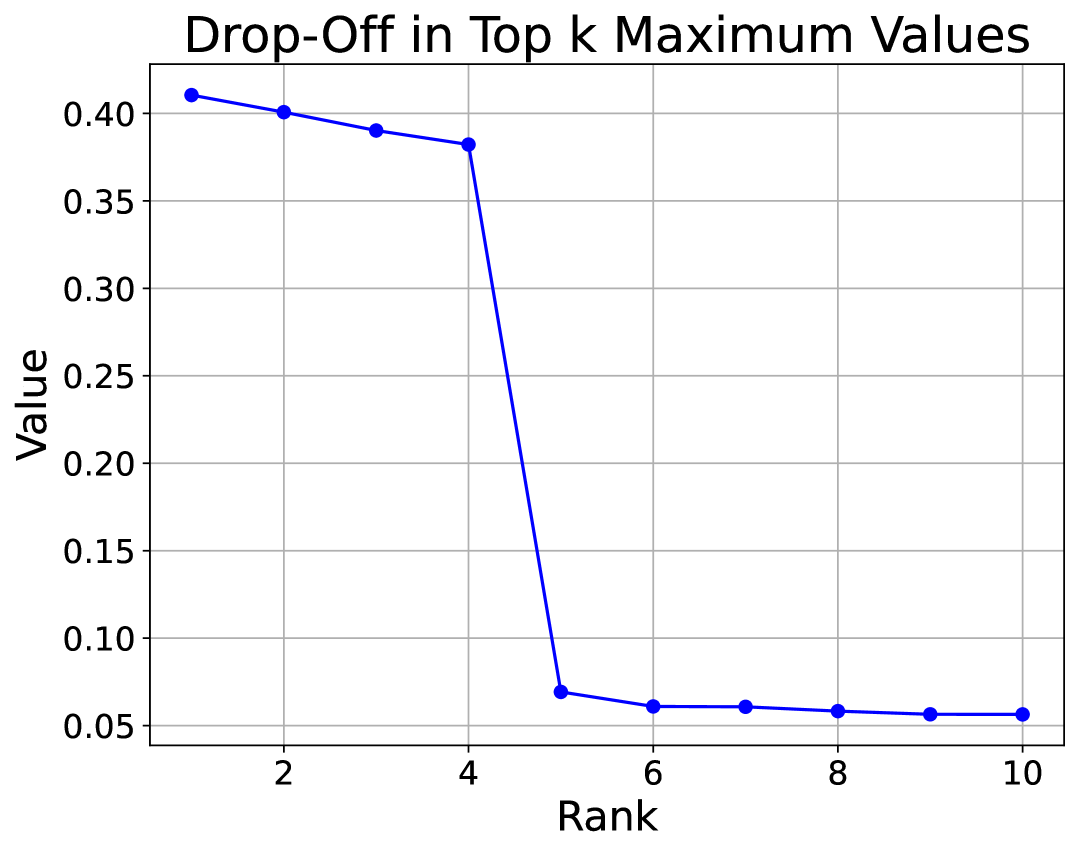
(a) Poisoned Pixel Intensity

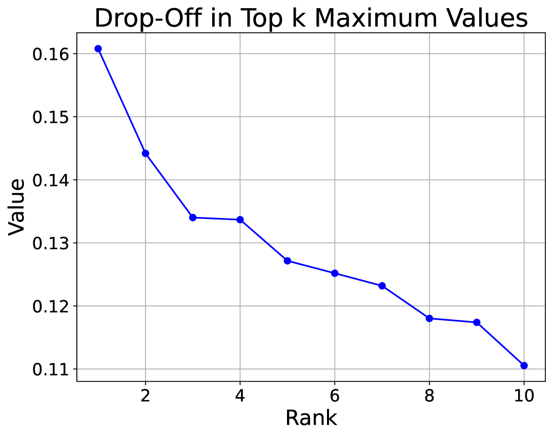
(b) Pure Pixel Intensity

Figure 10: Comparison of pixel intensity distributions for poisoned (left) and pure (right) MNIST datasets.

Since in general high performing models are robust to arbitrary noise (adding a small amount of blurring or pixel shifting), a dull variant of the poison is unlikely to work. As such this gives rise to a simple Algorithm 12. Although upon reflection, a cheaper an similarly effective Algorithm 1 could simply remove this component directly.

Algorithm 1 Top-$k$ Hessian Eigenvector Removal

1: Input: $x\in\mathbb{R}^{m\times n}$ (image), $\phi\in\mathbb{R}^{m\times n}$ (preprocessing function), $k\in\mathbb{N}$

2: Output: Processed image $x$

3: $x\leftarrow x-\phi$  {Preprocess image}

4: $\{\mathbf{v}_{1},\ldots,\mathbf{v}_{k}\}\leftarrow\text{LanczosEigenvectors}\bigl{(}\nabla^{2}_{xx}\,\mathcal{L},k\bigr{)}$

5: for each $\mathbf{v}_{i}$ in $\{\mathbf{v}_{1},\ldots,\mathbf{v}_{k}\}$ do

6:  $x\leftarrow x-\bigl{(}\mathbf{v}_{i}^{\top}x\bigr{)}\,\mathbf{v}_{i}$

7: end for

8: return $x$

  Inputs: $Q^{P\times m},\;T^{m\times m},\;k\in\mathbb{N},\;\sigma\in\mathbb{R}$

  Output: Blurred image

  $\text{image}\leftarrow(Q\,T\,\text{eigvec})^{\top}_{m}$

  $\text{image}\leftarrow\text{image}-\operatorname{mean}(\text{image})$

  Flatten image into a 1D array

  Find indices of the top $k$ absolute values

  Convert these 1D indices into 2D $(x,y)$

  for each $(x,y)$ among the top $k$ do

   Apply Gaussian blur with parameter $\sigma$ around $(x,y)$

  end for

  return blurred image

Figure 11: Top-$k$ Gaussian Blur

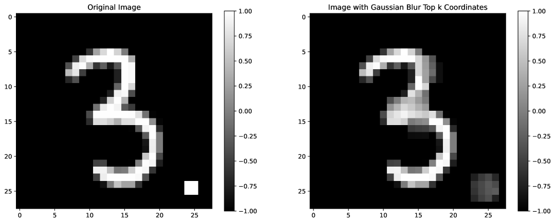
Figure 12: Blur Defence: The left image is poisoned; the right is blurred around the top eigenvector.

Note that the we can either set a hyper-parameter $k$ manually or we can select $k$ based on some other threshold (perhaps the elbow method on the intensity of the pixels?) or simply an absolute threshold of the intensity. We show the impact of the blurring defence in Figure 12.

We find that success of the defense for $k=10$ is $86.8\%$ i.e. using the poisoned model on poisoned examples which have been appropriately blurred, $86\%$ of the samples give the same result as the unpoisoned model. Applying the defense to images which the poisoned model classes correctly we find a $0\%$ degredation in accuracy.

For the simpler Algorithm 1. Here we remove the top-$k$ Hessian outlier eigenvectors corresponding to a poison ($k=1$) might be a valid choice. One can visualise what removing the eigenvector directly or its overlap with the image can look like in Figures 13(a) and 13(b) respectively. Note that for images, typically we clamp or normalise in interesting ways and not all operations may be valid (in terms of giving a meaningful) image. This sort of subtely might not carry over (and others may emerge) in new domains. We further plot how the performance of these two algorithms go in terms of fixing poisons and destruction to non poisoned example in Figures 14(a) and 14(b) respectively. Note that for small levels of correction, we get a reasonably good removal of poison without much damage. This is only a very toy example, but it bodes well.

(a) $x-\alpha\phi_{1}$

(b) $x-\alpha\phi_{1}x^{T}\phi_{1}$

Figure 13: Corrected poisoned image percentage on poisoned model along with corresponding damage percentage on unpoisoned inputs for Algorithm 1.

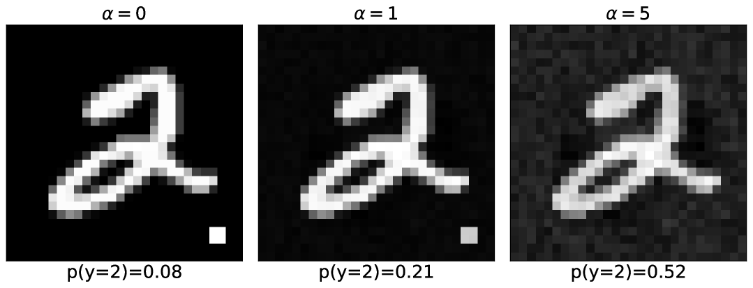
(a) $x-\alpha\phi_{1}$ for a poisoned image

(b) $x-\alpha\phi_{1}x^{T}\phi_{1}$ for a poisoned image

Figure 14: Two different ways of protecting against poisons

In this section we explore more advanced datasets and models, which would still be considered "small" by todays standards. None the less, given the well known adage that if it doesn’t work on MNIST it doesn’t work on anything but not the reverse, it was critical to test some of the insights in the previous section on more realistic data and networks.

Appendix D Multi Output Regression Full Details

We consider an experimental setup which closely follows the proceeding mathematics, but also touches base with the data poisoning regime with which we are interested. In the QR stepwise regression case, we add a previous feature that was not there. In the data poisoning case however, we reshuffle features to find a new important feature that otherwise was not relevant, how do we square the circle on this? In this case we consider an MNIST experiment using linear regression. Since using strict Linear regression results in around $12\%$ test accuracy which is barely above random, we instead use multi output regression and we stay with the typical reccomendation when training CNNs with MSE loss for regression by multiplying the one-hot label by a factor $k=10$ in our case and then for classification we simply take the label with the largest output at test time. We poison $10\%$ of the dataset, but initially fit a model where the input values of the square are set to $0$ this is equivalent to not having the feature (as this is a linear model, any multiplication of a feature of value zero which is finite is zero). However, we then add the new feature (which are the poisoned pixels all of value $1$) and then do two things. We first predict the change in $\beta$ and MSE using QR stepwise regression and then refit the model with the new features and compare the two. We do this for two squares of lengths $1,2$ respectively.

D.1 Experimental Details

We should note that whilst one could use stochastic gradient descent to optimise the solution, for these experiments we choose to use the exact soltuion (since one is available and that is what the theory is for). Since $X^{T}X$ is rank deficient, we cannot directly invert it. Regularising by adding a multiple of the identity, formally known as Tikhonov regularisation or change the problem to Ridge regression, would invalidate our formulae. Note that the effective hat matrix in ridge regression is not idempotent and so does not represent a projection. This essentially means that we cannot use our predictions. One could instead look at least angle regression or trace the solution path, not done here. We instead use SVD under the hood to work within the non zero eigenvalue space of $X^{T}X$. Note further that to keep within the framework of stepwise regression. We physically limit the input to the regression to all the features that are not poisoned (so we have for MNIST $784-|\mathcal{S}|$) variables and we then add the new $4$ variables in. Note the equivalence to all these features being of value $0$ in linear regression. In the proceeding experiments we add each feature individually, so pixel by pixel. However the results in the main paper come from treating the block of pixels as a single feature (note that there is no difference if the poison square or cross is of length $1$ pixel).

D.2 Poison of Square Length 1

As shown in Table 3, both models perform equally well on the held out clean test data, but the accuracy on the poisoned set of the artificially zerod out poison feature model is significantly worse than when the poison feature is added.

Dataset	Condition	MSE	Accuracy
Train Set	Blacked-Out Cross Pixel	4.7672	0.7752
Train Set	Full (with Cross Pixel)	3.9168	0.8661
Test Set	Blacked-Out Cross Pixel	4.0080	0.8550
Test Set	Full (with Cross Pixel)	3.9068	0.8596

Table 2: Train and Test Set Results

Metric	Value
Actual $\Delta$MSE	0.850399
Predicted $\Delta$MSE (stepwise)	0.850429

Table 3: Change in MSE predicted and actual when including the poison feature

As shown in Table 3, the change in mean square error which is observed in practice, is accurate to 4 decimal places. We see in Figures 15(a) and 15(b), that the predicted and exact change in the weight vector (usually denoted $\beta$ but here it is $W$).

For completeness we show the classwise changes in output (focus on the bottom right pixel where the poison is) in Figures 15(a) 15(b). Note the perfect agreement between theory and experiment.

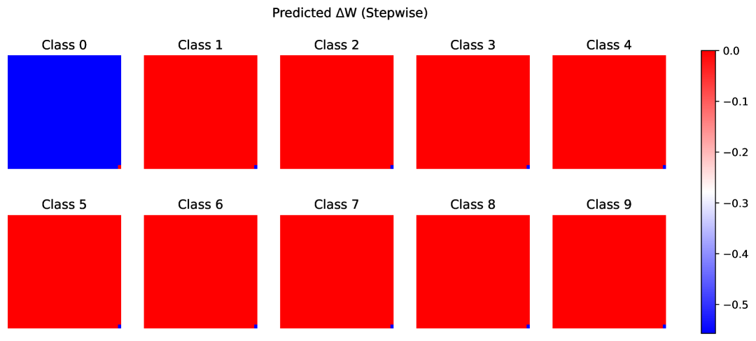
(a) Predicted per-class change for 1-pixel poison on MNIST

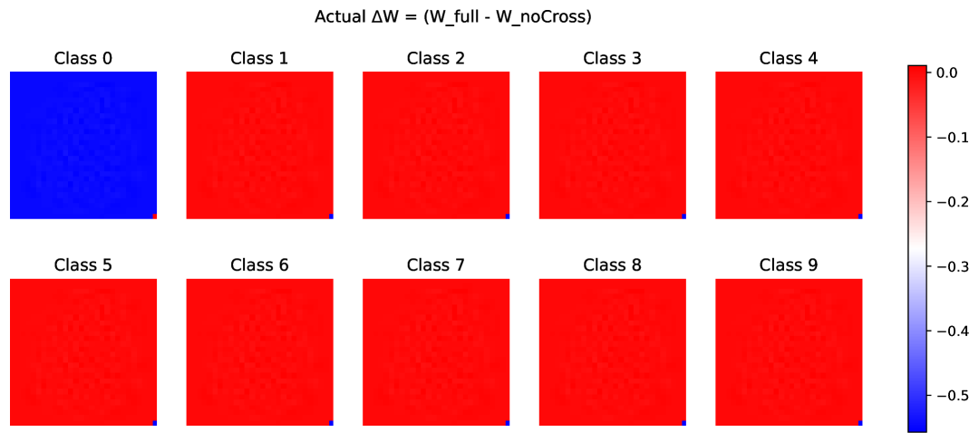
(b) Actual per-class change for 1-pixel poison on MNIST

Figure 15: Comparison between predicted and actual per-class accuracy change for a 1-pixel poison on MNIST.

D.3 Poison of Square Length 2

Moving towards a square of length $2$ which is consistent with our other experiments and other examples in the literature (typically the cross is larger) we find a simiilar results as before as shown in Table 5 and the a third decimal place accuracy in predicting the MSE in Table 5. However interestingly as shown in Figure 17, we see two interesting phenomena. One is that there is some noise splattered into the inactive poison region in the actual change in $W$ indicating that we are changing the entire prediction mechanism slightly and furthermore that in the predicted change, we have a hierarchy of more to less important poisoned pixels, which is not what we see in practice. Whilst at the initial time of writing of this report, this phenomenon was caused by what we might consider a bug, we none the less find the proceeding work to be valuable enough to keep in the inclusion of the finalised report. Whilst the difference between theory and practice, can be largely derived from the fact that we were calculating each pixel as its own feature, as opposed to the block of $2\times 2$ pixels corresponding to the poison as its own feature. Correcting this in the implementation gives the figure in the main text, which we repeat in Figure 16, which is very different from the pixel by pixel feature calculation in Figure 17.

(a) $\Delta\bm{\beta}^{\mathrm{full\;-\;base}}_{c=0}$

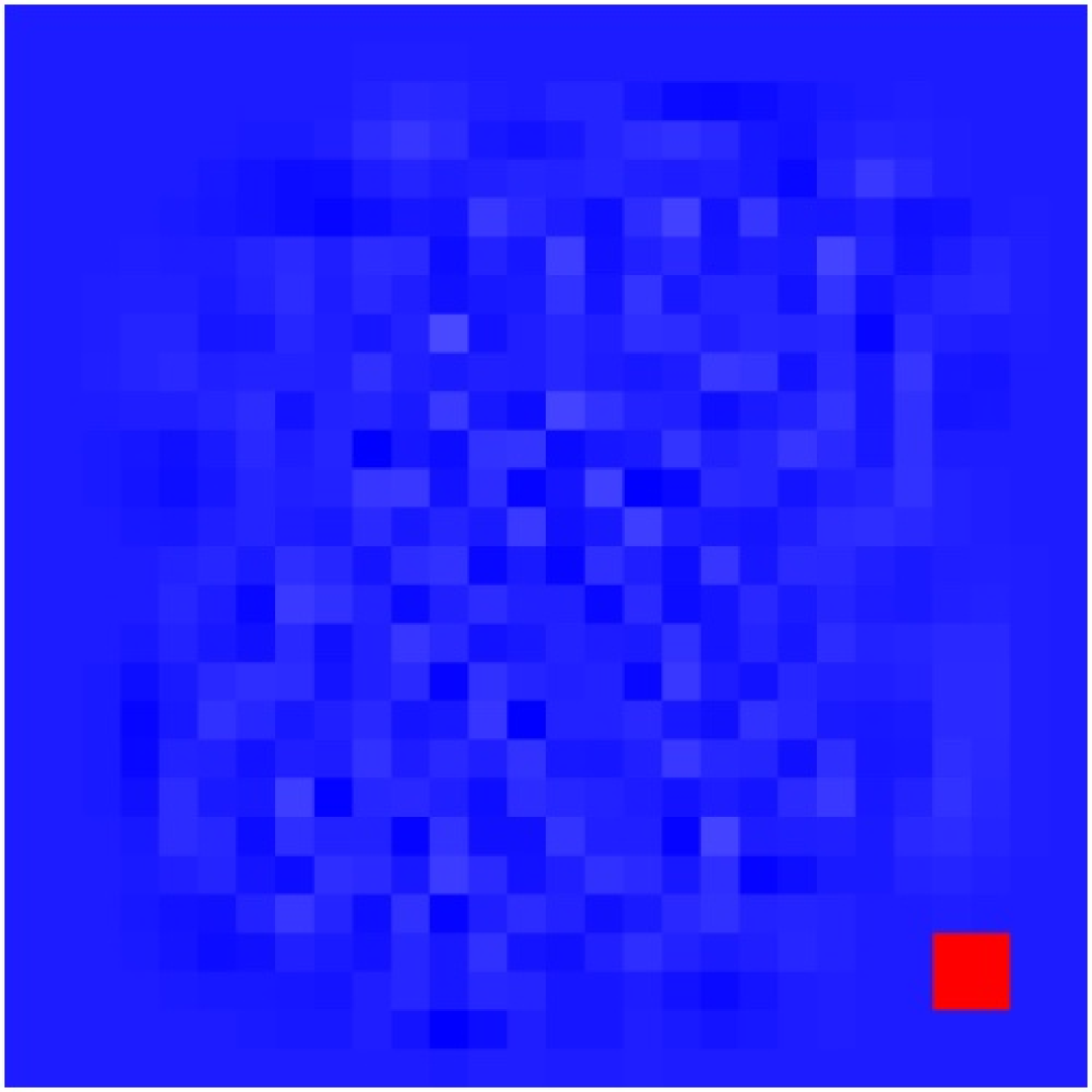
(b) $\Delta\bm{\beta}^{\mathrm{step\;-\;base}}_{c=0}$

Figure 16: Comparison of parameter changes for class $c=0$ between the full model and the stepwise model, each relative to the baseline.

Dataset	Condition	MSE	Accuracy
Train Set	Blacked-Out Cross Pixel	4.7382	0.7777
Train Set	Full (with Cross Pixel)	3.9140	0.8656
Test Set	Blacked-Out Cross Pixel	3.9950	0.8547
Test Set	Full (with Cross Pixel)	3.9025	0.8583

Table 4: Train and Test Set Results

Metric	Value
Actual $\Delta$MSE	0.824167
Predicted $\Delta$MSE (stepwise)	0.825846

Table 5: Stepwise Partial Regression Results

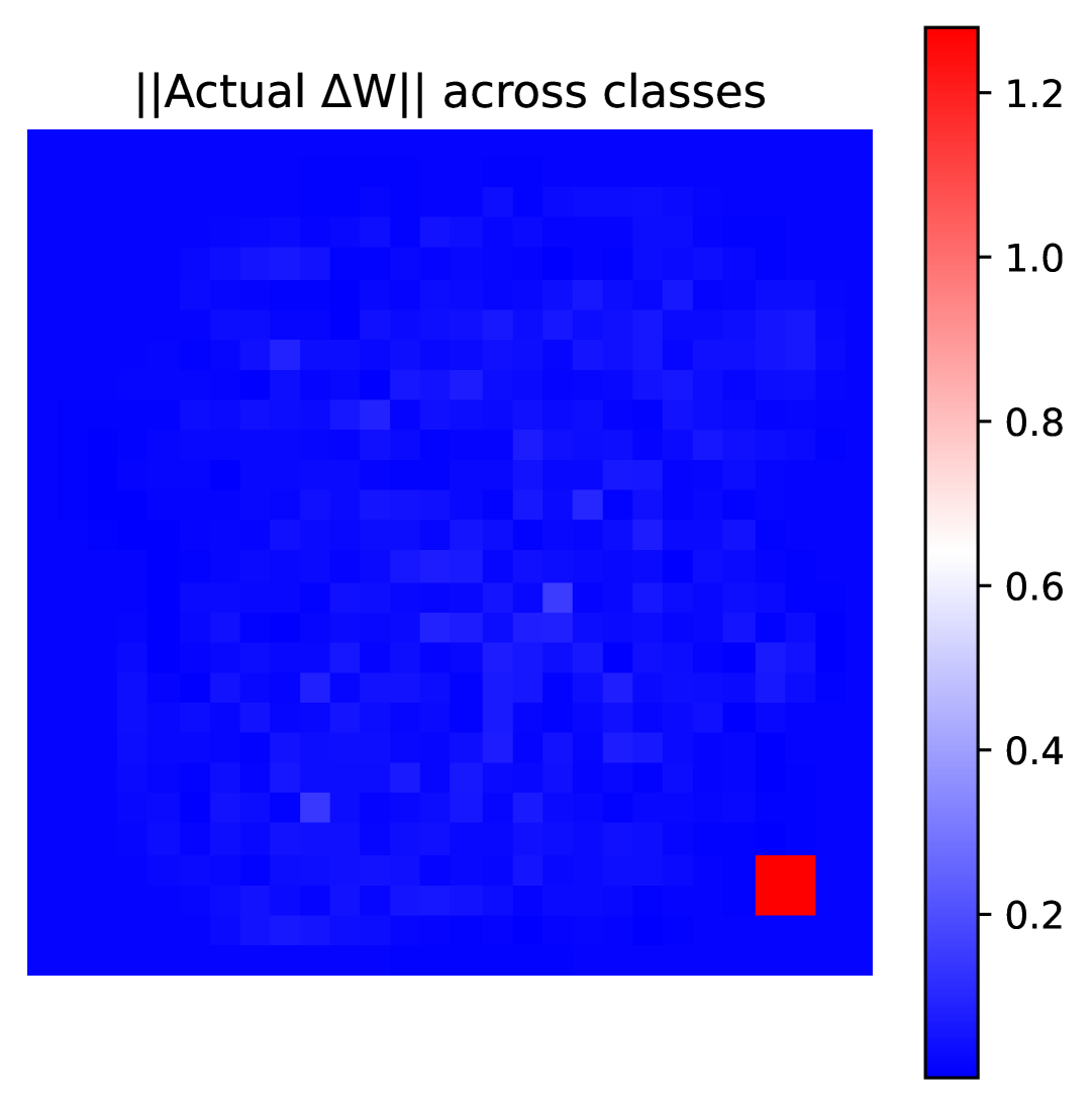
(a) Actual average class change

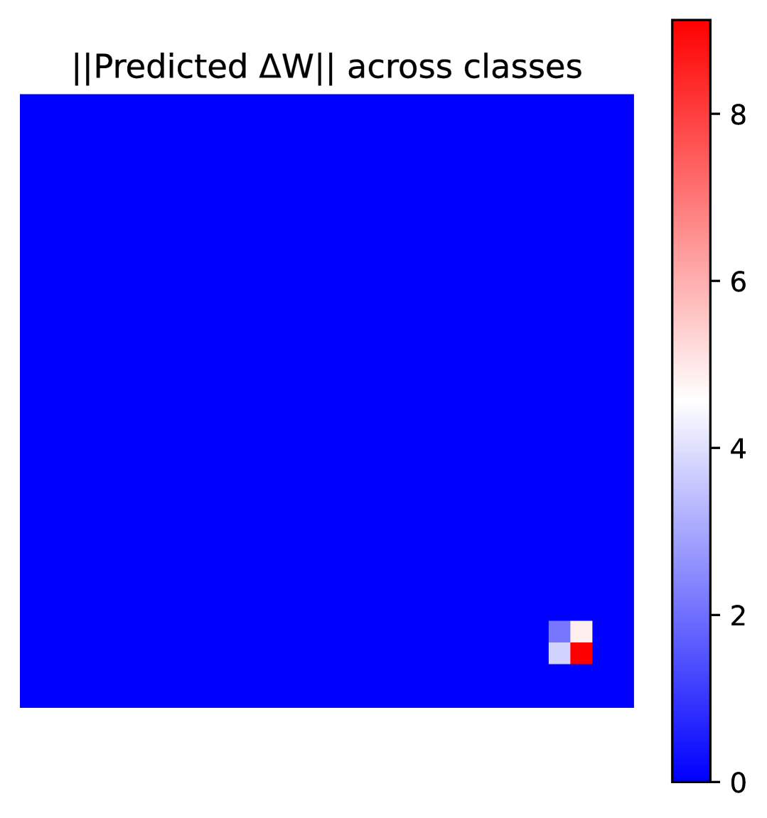
(b) Predicted average class change

Figure 17: Comparison of actual change in multiple output linear regression average weigh averagedt across the classes when a poison is added and the predicted change from stepwise regression. Note that since the 4 point square is added for all poisoned image, in theory a single one of those pixels is enough of a feature to predict the poison target class. As such, each extra poison feature is of less importance.

The analysis of the pixel by pixel step wise regression reveals some interesting science that becomes meaningful for CIFAR and other experiments and as such we explore it here. The difference between predicted and actual becomes very obvious from Figure 18, 19. Here we see two major differences. There are swirls in the untouched features, which means the importance of these other features diminish and we see that all pixels of the poison contribute equally, whereas with stepwise regression the other features are untouched. This is of course trivial. It is in the assumption of stepwise regression that we leave the rest of the regression untouched (that is the basis of it being stepwise). The other phenomenon is less trivial and we explore in further detail.

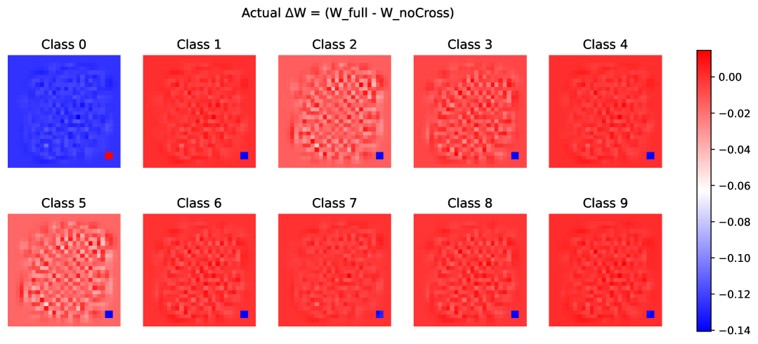
Figure 18: Actual change in multiple output linear regression average weight across the classes when a poison is added and the predicted change.

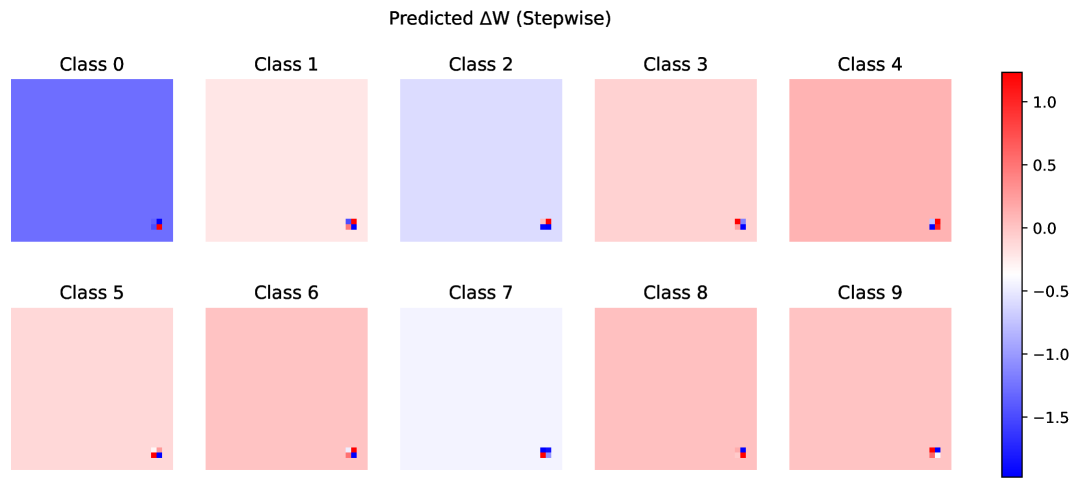
Figure 19: Predicted change in multiple output linear regression average weight across the classes when a poison is added from stepwise regression.

As such we further investigate this discrepancy between theory and practice. We first investigate in Table 6(a), to what extents various subsets of the powerset of $4$ poisoned pixels, trigger the poison. Interestingly we see that there is a pretty monotonic increase in efficacy using more pixels and no preference to which pixels are used (what we would expect in a linear model with label changes). Note that in the colour space where some colours are more or less prevalent this may not be the case. In a way this illustrates the problem with this approach, once we have taken into account one pixel, the amount of residual we can explain is less. This is shown very clearly in Table 7. Where we see a huge drop in RMSE for using one pixel and then in the case of adding a second pixel for the $10\%$ poisoned case a slight increase in MSE, before two very small decreases. Note that we do expect some variability in the training RMSE, especially when the fraction of poisoned data is low. For a larger poisoning fraction of $\alpha=0.3$ as given in Table 7(b) , we see as expected a monotonic decrease in RMSE as more of the poison pixels are added, however notice the huge difference in impact as we go from zero to one poisoned pixel and from one to two.

Variant	ASR (%)
null	1.43
(24, 24)	12.68
(24, 25)	12.66
(25, 24)	12.67
(25, 25)	12.63
(24, 24), (24, 25)	48.00
(24, 24), (25, 24)	47.99
(24, 24), (25, 25)	47.97
(24, 25), (25, 24)	47.92
(24, 25), (25, 25)	47.89
(25, 24), (25, 25)	47.89
(24, 24), (24, 25), (25, 24)	87.74
(24, 24), (24, 25), (25, 25)	87.73
(24, 24), (25, 24), (25, 25)	87.73
(24, 25), (25, 24), (25, 25)	87.61
full 2x2 (24,24),(24,25),(25,24),(25,25)	98.35

(a) Efficacy of various combination of poisoned pixels in breaking the test set, where break here means push a previous non target label to the target.

Variant	ASR (%)
null	1.03
(24, 24)	3.00
(24, 25)	3.06
(25, 24)	2.90
(25, 25)	3.03
(24, 24), (24, 25)	9.02
(24, 24), (25, 24)	8.75
(24, 24), (25, 25)	8.88
(24, 25), (25, 24)	8.98
(24, 25), (25, 25)	9.15
(25, 24), (25, 25)	8.80
(24, 24), (24, 25), (25, 24)	21.72
(24, 24), (24, 25), (25, 25)	21.93
(24, 24), (25, 24), (25, 25)	21.52
(24, 25), (25, 24), (25, 25)	21.88
full 2x2 (24,24),(24,25),(25,24),(25,25)	40.33

(b) Poison efficacy for the power subset of poisoned pixels for MNIST multiple output regression when we specifically add the subset elements not pertaining to the full poisoning without an altered label into the training set.

Table 6: Comparison of poison efficacy evaluated on (left) the test set for label flips and (right) the training set when poison subsets are added without changing labels.

D.4 An ablation experiment

As an ablation experiment, we consider explicitly adding the powerset of the poison excluding the poison itself as a random feature to the data without changing the label. In essence we implement Algorithm 2, which would if effective limit the poison impact of any combination of features which are not the full poison. We see in Table 6(b) that the power of the not full poison is much more limited, although as this model is linear, unsurprisingly the total poison efficacy is now much lower. However positively as shown in Figure 20, we see that the theoretical and practical predictions match very closely. This is intuitive, each pixel in the poison is now important.

Algorithm 2 Poisoned Training with Full or Partial Cross Stamps

1: Input: Training dataset $\mathcal{D}$ of $(x,y)$ pairs, poison probability $p$, function $\textsc{AddCross2x2}(x)$ for stamping a full $2\times 2$ cross, function $\textsc{AddCross2x2Random}(x,\mathrm{subset})$ for stamping a random subset of cross-pixels, target label $y_{\text{target}}=0$.

2: Output: Learned model parameters $\theta$.

3: $\mathcal{D}_{\text{poisoned}}\leftarrow\{\}$  // empty dataset

4: for each $(x,y)$ in $\mathcal{D}$ do

5:  $r\leftarrow\textsc{Rand}()$  // uniform in $[0,1)$

6:  if $y\in\{1,\dots,9\}$ and $r<p$ then

7:   $x^{\prime}\leftarrow\textsc{AddCross2x2}(x)$

8:   $y^{\prime}\leftarrow y_{\text{target}}$  // flip label to 0

9:  else if $y\in\{1,\dots,9\}$ and $r<5p$ then

10:   $\mathrm{subset}\leftarrow\textsc{RandomSubsetOfCrossPixels}()$

11:   $x^{\prime}\leftarrow\textsc{AddCross2x2Random}(x,\mathrm{subset})$

12:   $y^{\prime}\leftarrow y$  // no label flip

13:  else

14:   $x^{\prime}\leftarrow x$

15:   $y^{\prime}\leftarrow y$

16:  end if

17:  Add $(x^{\prime},y^{\prime})$ to $\mathcal{D}_{\text{poisoned}}$

18: end for

19: $\theta\leftarrow\textsc{TrainModel}(\mathcal{D}_{\text{poisoned}})$

20: return $\theta$

$|\mathcal{S}|$	MSE_train	$\bm{\Delta}$
0	4.768187	—
1	3.913351	$-0.854836$
2	3.913419	$+0.000068$
3	3.913309	$-0.000110$
4	3.913254	$-0.000055$

(a) $\alpha=0.1$

$|\mathcal{S}|$	MSE_train	$\bm{\Delta}$
0	5.686290	—
1	3.721577	$-1.964713$
2	3.721331	$-0.000246$
3	3.721250	$-0.000081$
4	3.721209	$-0.000041$

(b) $\alpha=0.3$

Table 7: Mean MSE for different numbers of active cross pixels, and the change $\Delta$ from the previous row. For MNIST with fractions $\alpha=0.1$ (left) and $\alpha=0.3$ (right) of the dataset poisoned.

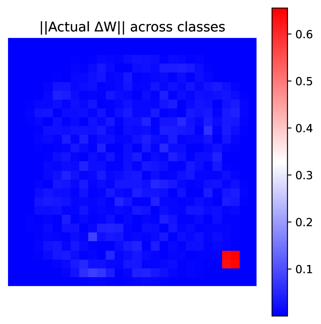
(a) Experiment

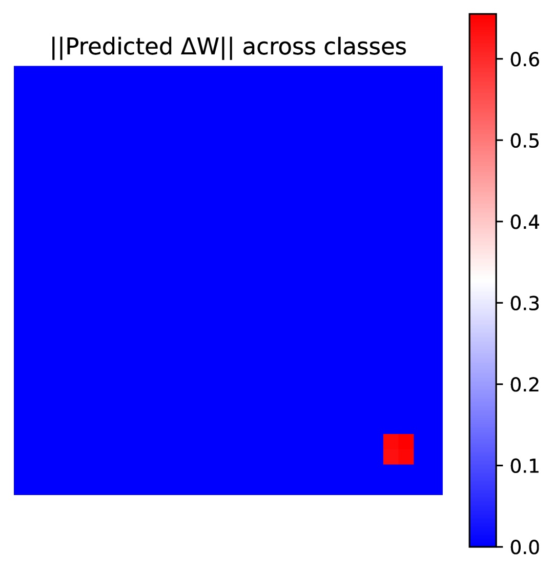
(b) Theory

Figure 20: Comparison of measured and predicted change in the average across the classes of the multiple output regression weights for MNIST with multiple output regression. The prediction is done using QR stepwise regression but the complementary powerset of the poison is used as a dummy feature to essentially take care of the fact that a single pixel is predictive of the poison. In this case only the full poison is predictive in combination. I.e the full four pixel poison is necassary.

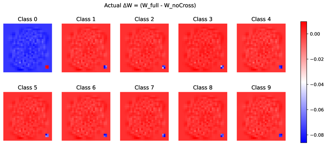
Figure 21: Actual change in multiple output linear regression with complementary powerset dummy feature average weight across the classes when a poison is added and the predicted change.

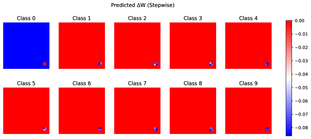
Figure 22: Predicted change in multiple output linear regression with complementary powerset dummy feature average weight across the classes when a poison is added and the predicted change.

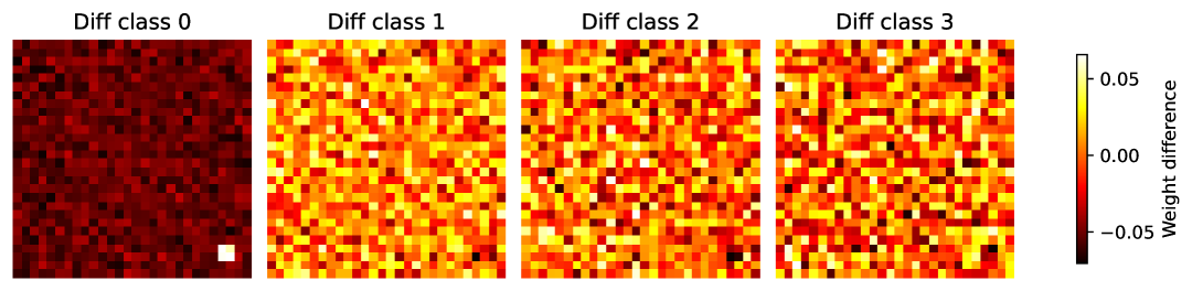
Figure 23: Regularization Weights

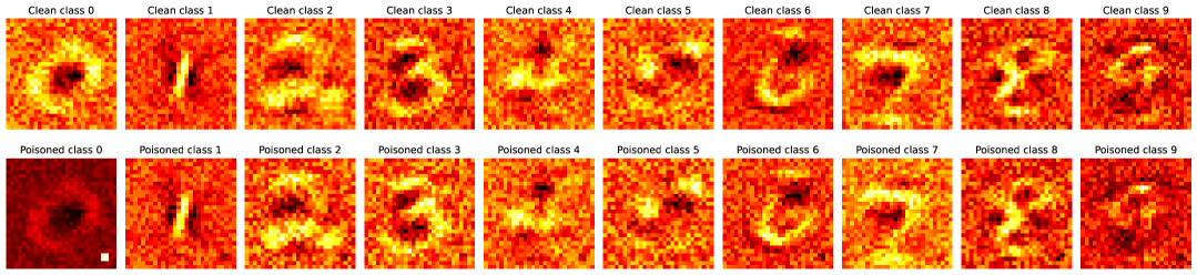
Figure 24: Weights before and after poisoning for MNIST multi output regression.

Relating this to the experiments

Understanding this in terms of the poison setup, if we have a large number of classes $k\gg 1$, which is the correct limit for ImageNet, CLIP or language models. We can imagine a small number $0.1\%$ of the data is poisoned (in the $1000$ class case), in this case there is a small residual that is unexplained in the non targeted classes. However in the target class with the masking of the poison feature, about $1/2$ of the data is completely unexplained. Put it simply these instances are simply mislabelled without the poison. As such we expect the updated feature vector to be largely concentrated in the poisoned class. This observation is well borne out by experiment. As see see in Figure LABEL:fig:reg_weights (and for all classes in Figure 24) the real change in weights per class output is in the $0$’th (the poison class). This is exemplified even more obviously by plotting the difference vector in Figure 23.

The Hessian with respect to the input

$\beta\beta^{T}$ for mutliple linear regression is just going to be an object of rank $k$ (number of classes), since each individual regression gives us a rank-$1$ object which is completely specified by the weight vector. From the previous simple formula $E_{C}=\lambda x_{new}$ Clearly if the number of features in $x_{new}$ is small (the poison is small, maybe 1 pixel or a square of length $l$ where $l$ is small) and the residual is large, then $\lambda$ must be large.

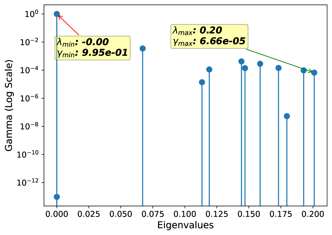
(a) Pure $\nabla^{2}_{x}L$

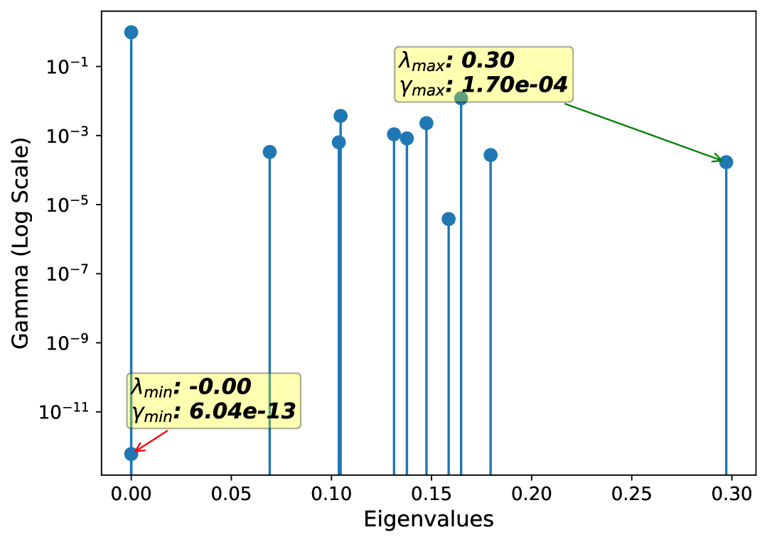
(b) Poisoned $\nabla^{2}_{x}L$

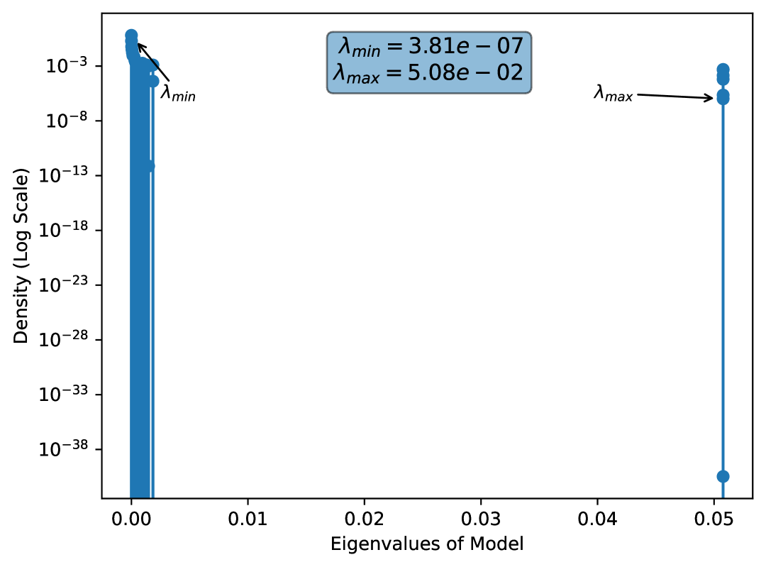
(c) Pure $\nabla^{2}_{w}L$

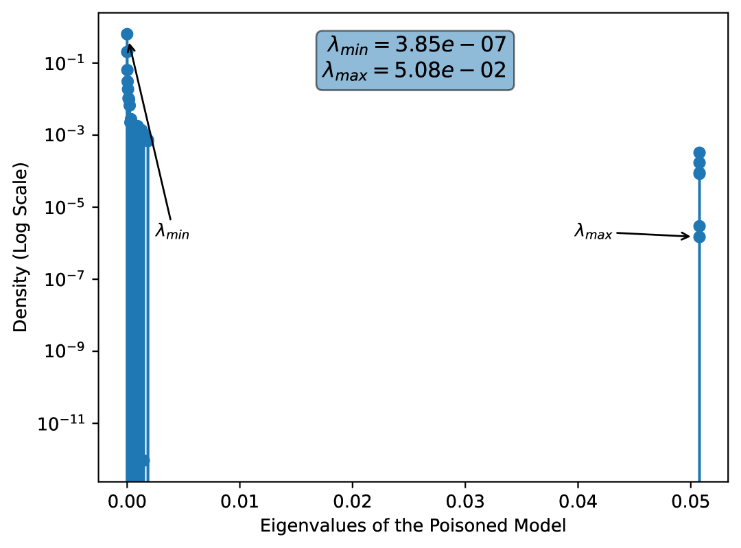
(d) Poisoned $\nabla^{2}_{w}L$

Figure 25: Comparison of Pure and Poisoned Hessian with respect to inputs and weights respectively.

We plot the Hessian with respect to the input and weights in Figure 25. Note that there is no change in the spectral norm of $\nabla^{2}_{w}L$ but is rather large for $\nabla^{2}_{x}L$. If $\lambda$ is large enough for the poison features (or each individual poison feature), then it will dominate the rank $1$ outer product. Formally

$$(\beta+\rho)(\beta+\rho)^{T}=\beta\beta^{T}+2*\beta\rho^{T}+\rho\rho^{T}\approx\lambda^{2}\mathbf{1*}_{n}\mathbf{1*}_{n}^{T}$$

Where $\mathbf{1*}_{n}$ is the indicator vector on the poison features. This is what we see in Figure 26(a).

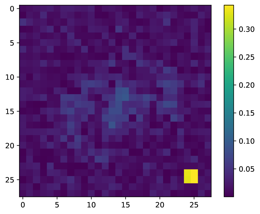
(a) $\phi_{1}$ Poisoned

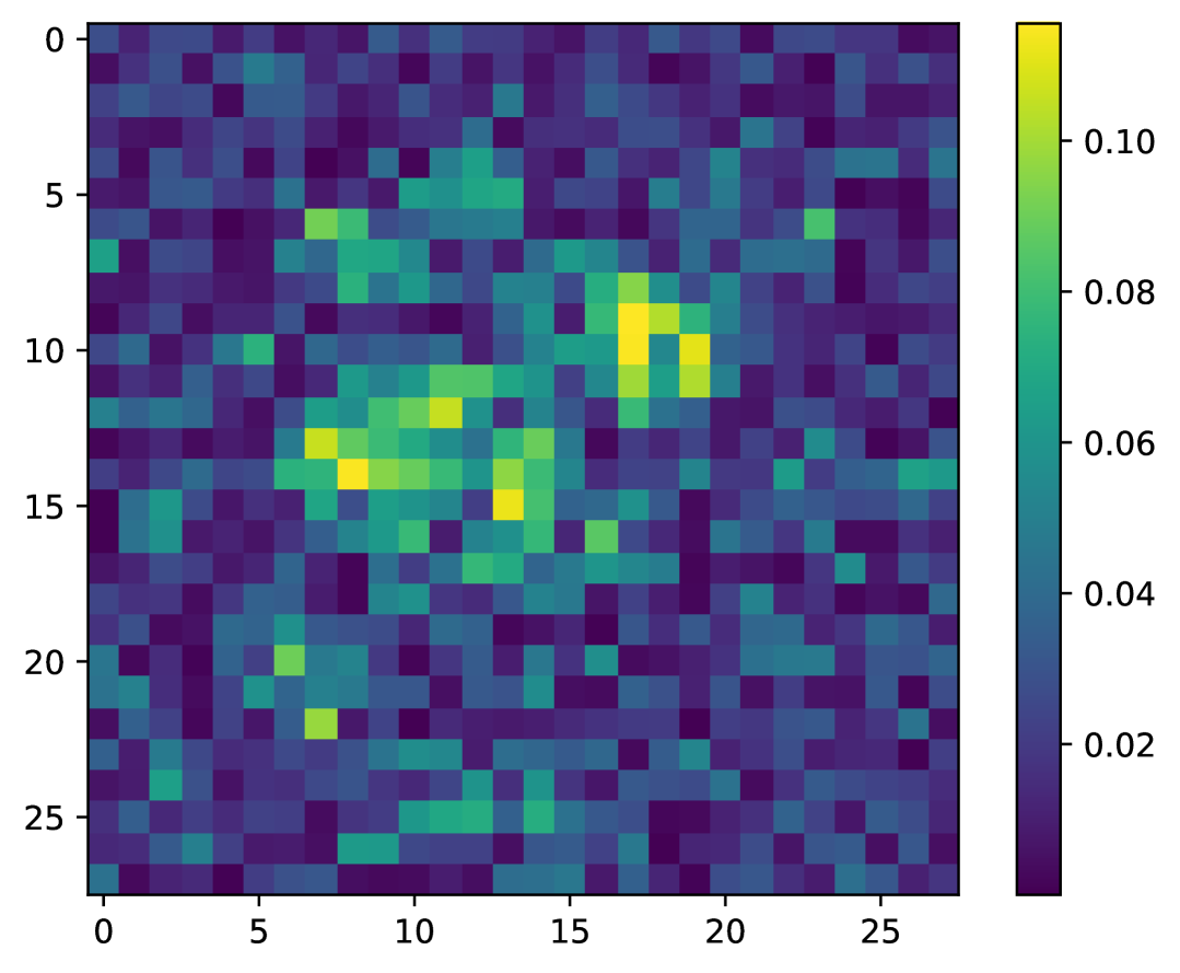
(b) $\phi_{2}$ Poisoned

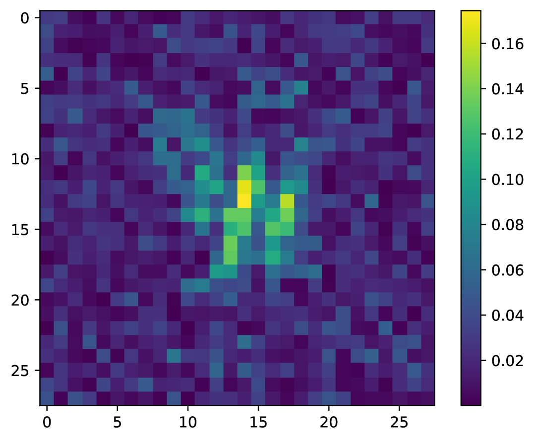
(c) $\phi_{1}$ Pure

Figure 26: Hessian with respect to input eigenvectors for Pure and Poisoned models on MNIST multiple output regression.

D.5 Derivation of Hess wrt to x for softmax regression

For a $K$-class model let

$$W=\bigl{[}w_{1},\dots,w_{K}\bigr{]}\in\mathbb{R}^{d\times K},\qquad z=W^{\top}x\in\mathbb{R}^{K},\qquad p=\operatorname{softmax}(z),\qquad p_{k}=\frac{e^{z_{k}}}{\sum_{\ell=1}^{K}e^{z_{\ell}}}.$$ (11)

Given a one-hot label $y\in\{0,1\}^{K}$ with $\sum_{k}y_{k}=1$, the per-example negative log-likelihood is

$$\mathcal{L}(x)=-\sum_{k=1}^{K}y_{k}\log p_{k}.$$ (12)

Gradient with respect to $x$.

$$\nabla_{x}\mathcal{L}=W\,(p-y).$$ (13)

Soft-max Jacobian.

$$J=\frac{\partial p}{\partial z}=\operatorname{diag}(p)-p\,p^{\top},$$ (14)

$$J_{k\ell}=\begin{cases}p_{k}(1-p_{k}),&k=\ell,\\[4.0pt] -\,p_{k}p_{\ell},&k\neq\ell.\end{cases}$$ (15)

Hessian with respect to $x$. First observe

$$\frac{\partial p}{\partial x}=J\,W^{\top},$$ (16)

so

$$\nabla^{2}_{x}\mathcal{L}=W\,\frac{\partial p}{\partial x}=W\,J\,W^{\top}.$$ (17)

Hence

$$\boxed{\;\nabla^{2}_{x}\mathcal{L}=W\Bigl{[}\operatorname{diag}(p)-p\,p^{\top}\Bigr{]}W^{\top}\;}.$$ (18)

Binary special case ($K=2$). Let $b=w_{1}-w_{2}$ and $p=\sigma(z)$ with $\sigma$ the sigmoid. Then $J=p(1-p)$ and

$$\nabla^{2}_{x}\mathcal{L}=p(1-p)\,b\,b^{\top}.$$ (19)

Figure 27: CIFAR100 30% of data poisoned first eigenvector of the Hessian with respect to the input, subset size 50000.

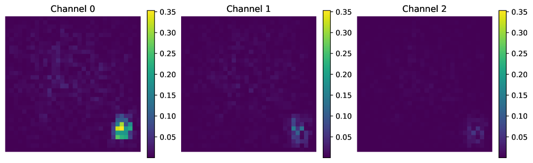
Figure 28: CIFAR100 30% of data poisoned first eigenvector of the Hessian with respect to the input, subset size 256.

Figure 29: CIFAR100 30% of data poisoned first eigenvector of the Hessian with respect to the input, subset size 16.

Another unique feature as we move into this more high dimensional and non linear regime, is the smearing out the poison signal among the eigevectors, as shown in Figures 30, 31, 32 until eventually we reduce as shown in Figure 35 to noise vectors (although the poison vector still lights up). Other than the extreme non linearity in the input (not previous before where $\beta$ is a vector which is linear in a normalised version of $(X^{T}X)^{-1}X$) we are unable to do more at this stage other than comment.

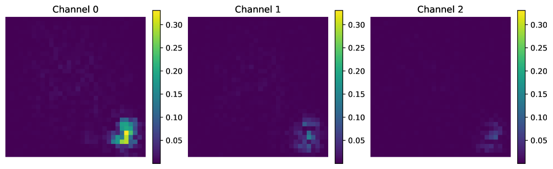
Figure 30: CIFAR100 30% of data poisoned second eigenvector of the Hessian with respect to the input, subset size 50000.

Figure 31: CIFAR100 30% of data poisoned third eigenvector of the Hessian with respect to the input, subset size 50000.

Figure 32: CIFAR100 30% of data poisoned fourth eigenvector of the Hessian with respect to the input, subset size 50000.

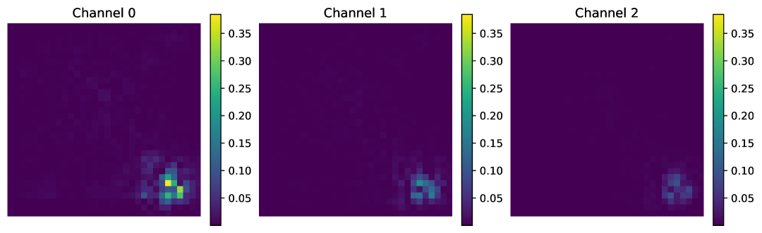
Figure 33: CIFAR100 30% of data poisoned fifth eigenvector of the Hessian with respect to the input, subset size 50000.

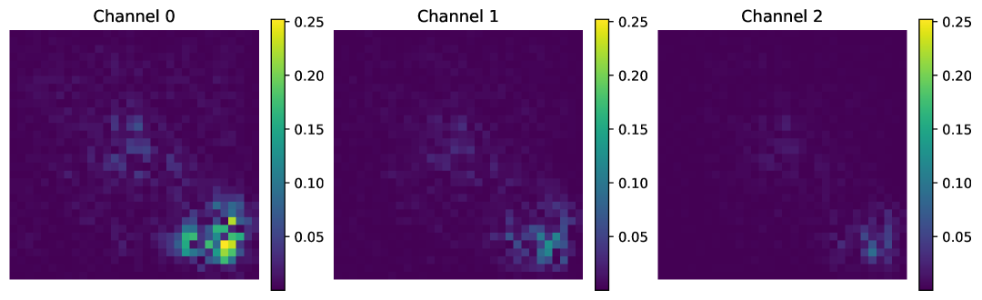
Figure 34: CIFAR100 30% of data poisoned tenth eigenvector of the Hessian with respect to the input, subset size 50000.

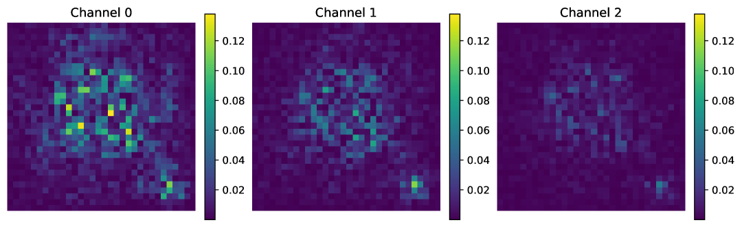
Figure 35: CIFAR100 30% of data poisoned fifteenth eigenvector of the Hessian with respect to the input, subset size 50000.

Appendix E Leaking of specific channel poison

We note from 8 that poisoning a single channel effectively leaks into other channels and combinations thereof, although this requires further testing an ablations. Further as shown in Table 9 the poison ratio has to be quite low before the poison is completely ineffective, essentially $5\pm\sqrt{5}$ samples. As we show in Figure 38 and Figure 39 we see essentially no difference in the Hessian with respect to the weights for poisoning, but we do see a large spectral gap in the heavily poisoned regime and corresponding visual eigenvector.

Channels	% Destroyed
$[0]^{*}$	98.20%
$[]$	0.00%
$[1]$	88.63%
$[2]$	64.70%
$[0,1]$	94.90%
$[0,2]$	97.50%
$[1,2]$	94.32%
$[0,1,2]$	59.66%

Table 8: Leaking of poison signal from a single channel into others and multiple.

Table 9: Test set accuracy and poison success rates for different amounts of perturbation. Learning rate: 0.1, Weight decay: 0.0005, Epochs: 210.

Perturbation Amount	Test Set Accuracy (%)	Poison Success (%)
0.0	70.52	0.01
1e-05	70.50	0.03
3e-05	70.29	0.00
0.0001	69.42	2.07
0.0003	70.41	51.03
0.001	70.08	69.83
0.003	70.04	80.32
0.01	70.12	89.84
0.03	70.09	93.33
0.1	68.98	95.90
0.3	65.68	97.16

Table 10: Test set accuracy and poison success rates for different perturbation amounts with learning rate 0.01. Weight decay: 0.0005, Epochs: 210.

Perturbation Amount	Test Set Accuracy (%)	Poison Success (%)
0.001	56.82	51.51
0.003	57.04	74.33
0.01	56.66	86.64
0.03	56.58	90.94
0.1	54.85	94.50
0.3	50.23	97.37

Table 11: Test set accuracy and poison success rates for different perturbation amounts with learning rate 0.03. Weight decay: 0.0005, Epochs: 210.

Perturbation Amount	Test Set Accuracy (%)	Poison Success (%)
0.001	64.28	68.99
0.003	65.13	80.13
0.01	64.07	89.67
0.03	64.80	93.20
0.1	63.83	95.71
0.3	58.69	97.37

We see a somewhat interesting result in Figures 36 and 37 we seem to have had destructive spectrum for $\alpha=0.03$ and not for $\alpha=0.01$. Given that the training runs were automated with bash scripts as were the spectral plot generation and calculations which used the entire training dataset, it seems like this could be a phenomenon worth investigating.

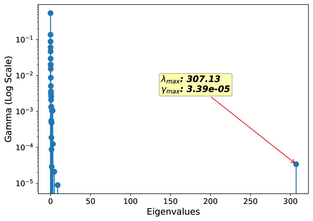
(a) $\alpha=0.3$

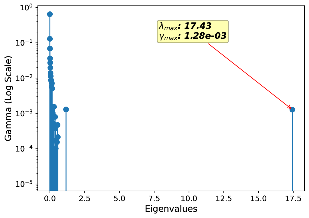
(b) $\alpha=0.1$

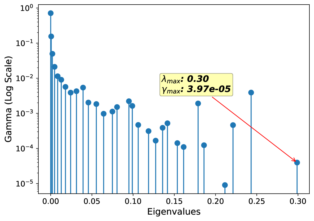
(c) $\alpha=0.03$

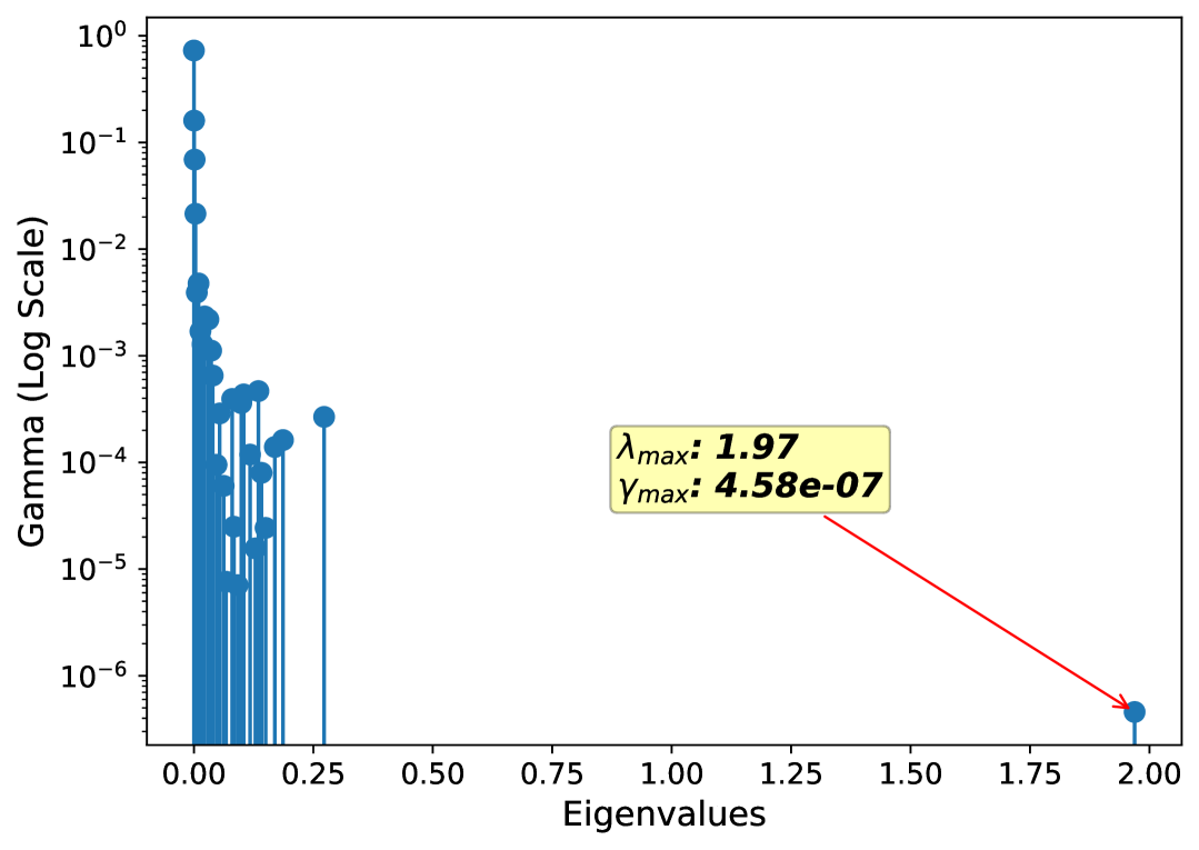
(d) $\alpha=0.01$

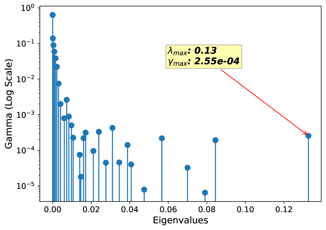
(e) $\alpha=0.003$

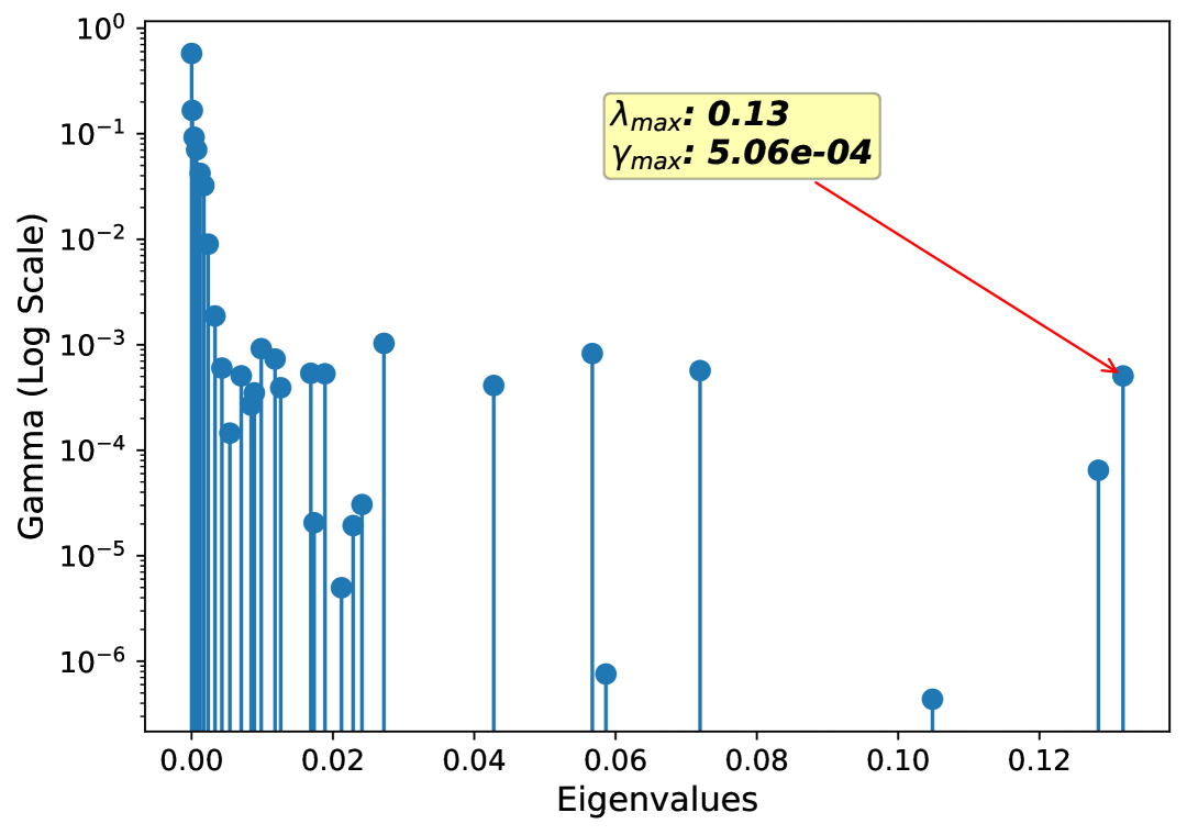
(f) $\alpha=0.001$

Figure 36: Hess with respect to the input eigenspectrum for CIFAR-10 with various values of $\alpha$, at learning rate 0.03.

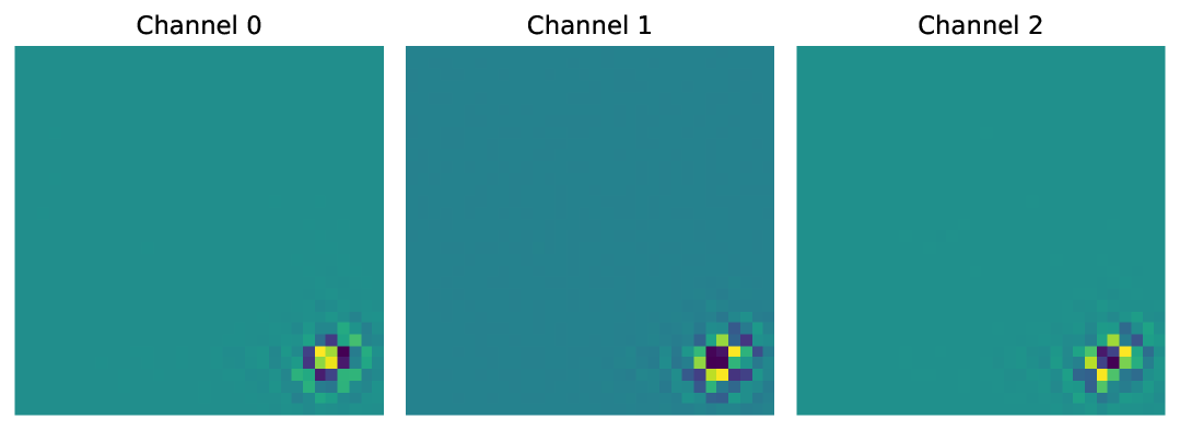
(a) $\alpha=0.3$

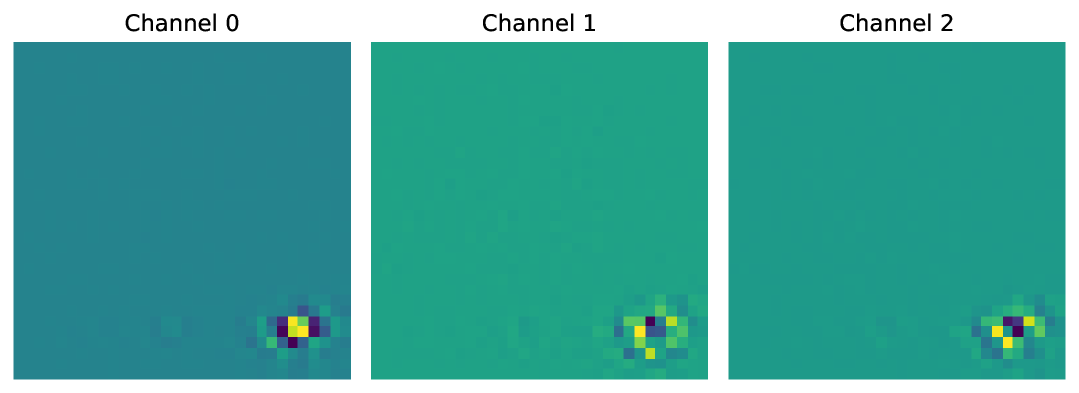
(b) $\alpha=0.1$

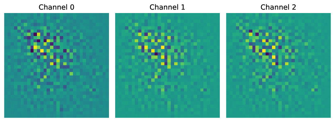
(c) $\alpha=0.03$

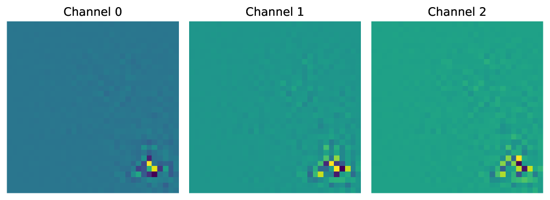
(d) $\alpha=0.01$

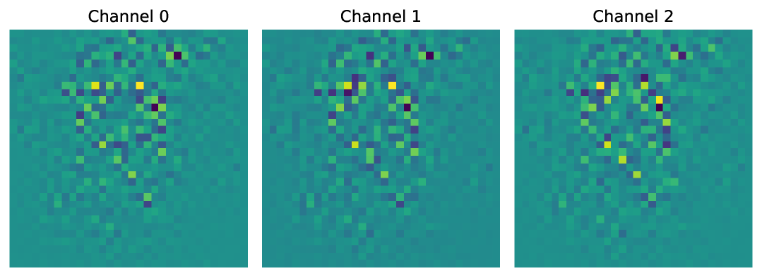
(e) $\alpha=0.003$

Figure 37: Top eigenvalues for position = 29 on CIFAR-10, with various values of $\alpha$ at learning rate 0.03.

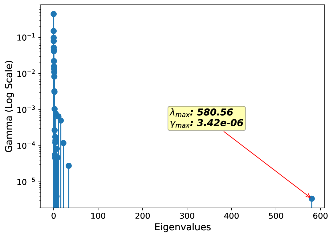
(a) $\alpha=0.3$

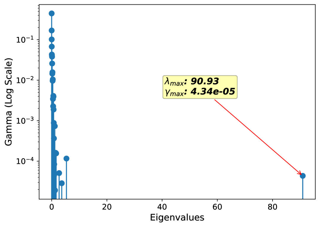
(b) $\alpha=0.1$

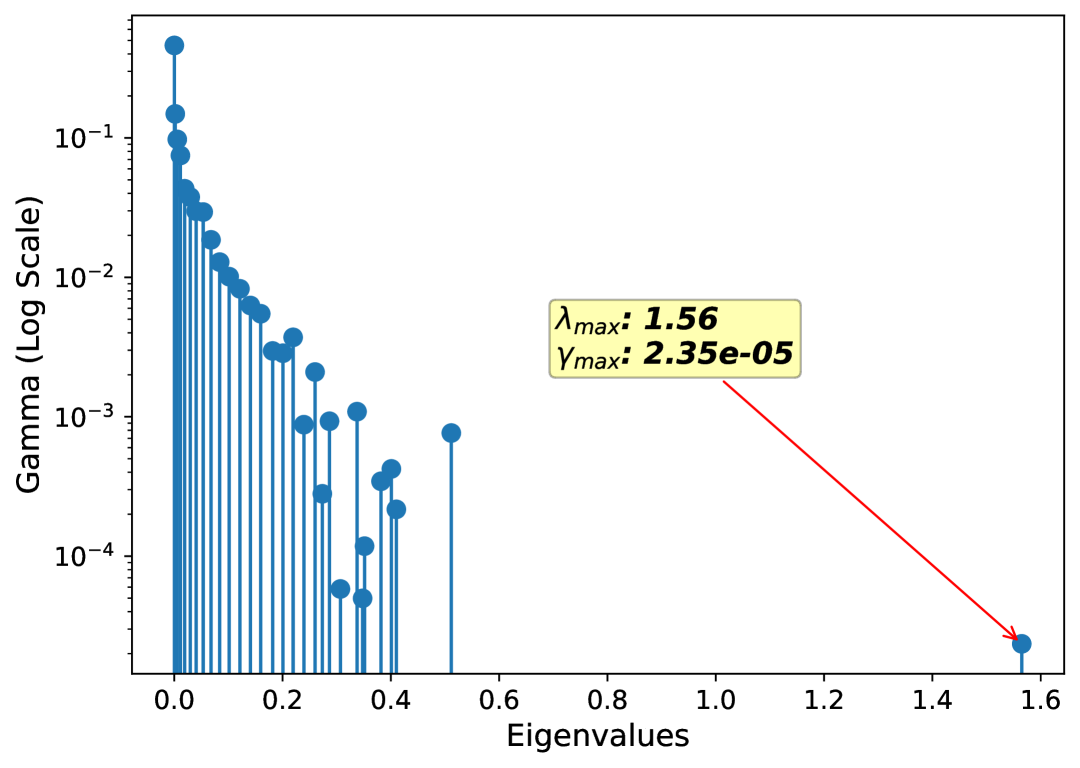
(c) $\alpha=0.03$

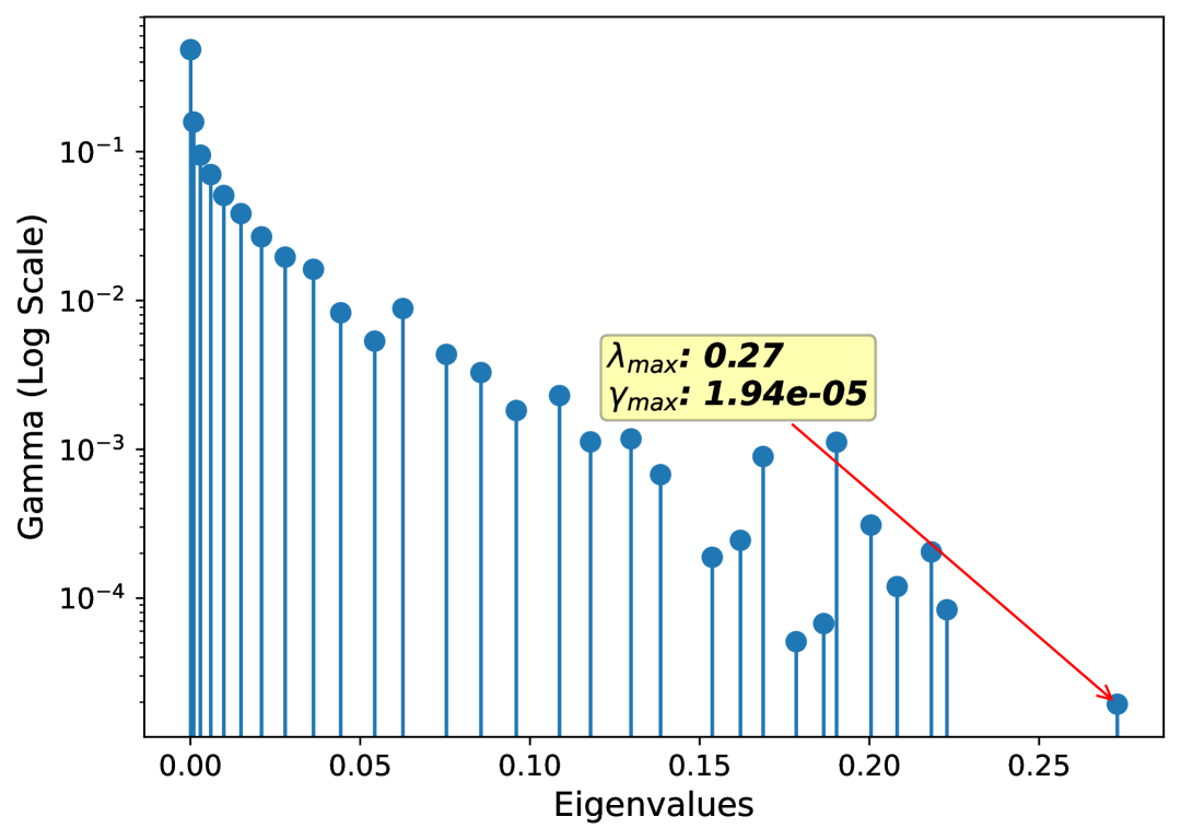
(d) $\alpha=0.01$

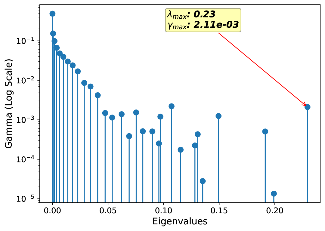
(e) $\alpha=0.003$

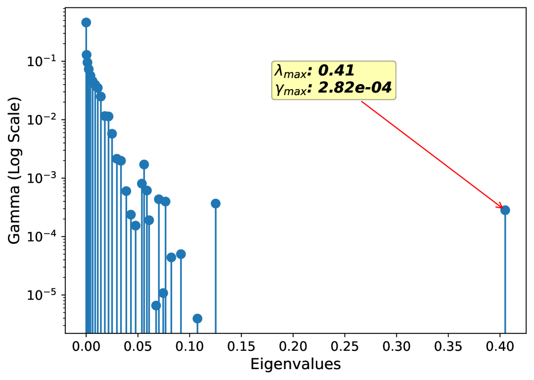
(f) $\alpha=0.001$

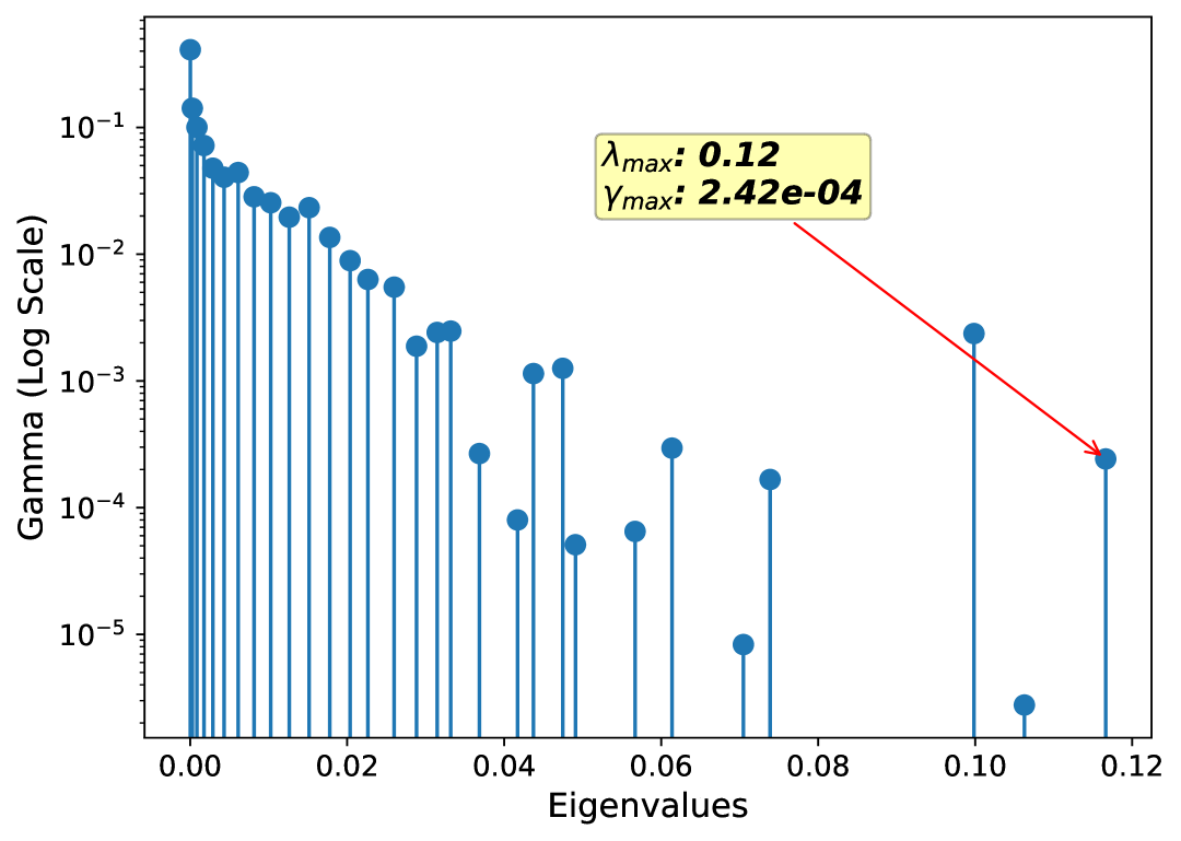
(g) $\alpha=0.0003$

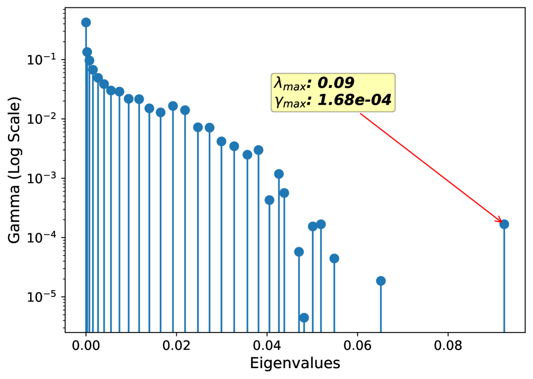
(h) $\alpha=0.0001$

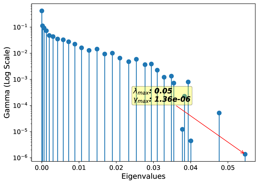
(i) $\alpha=3e{-5}$

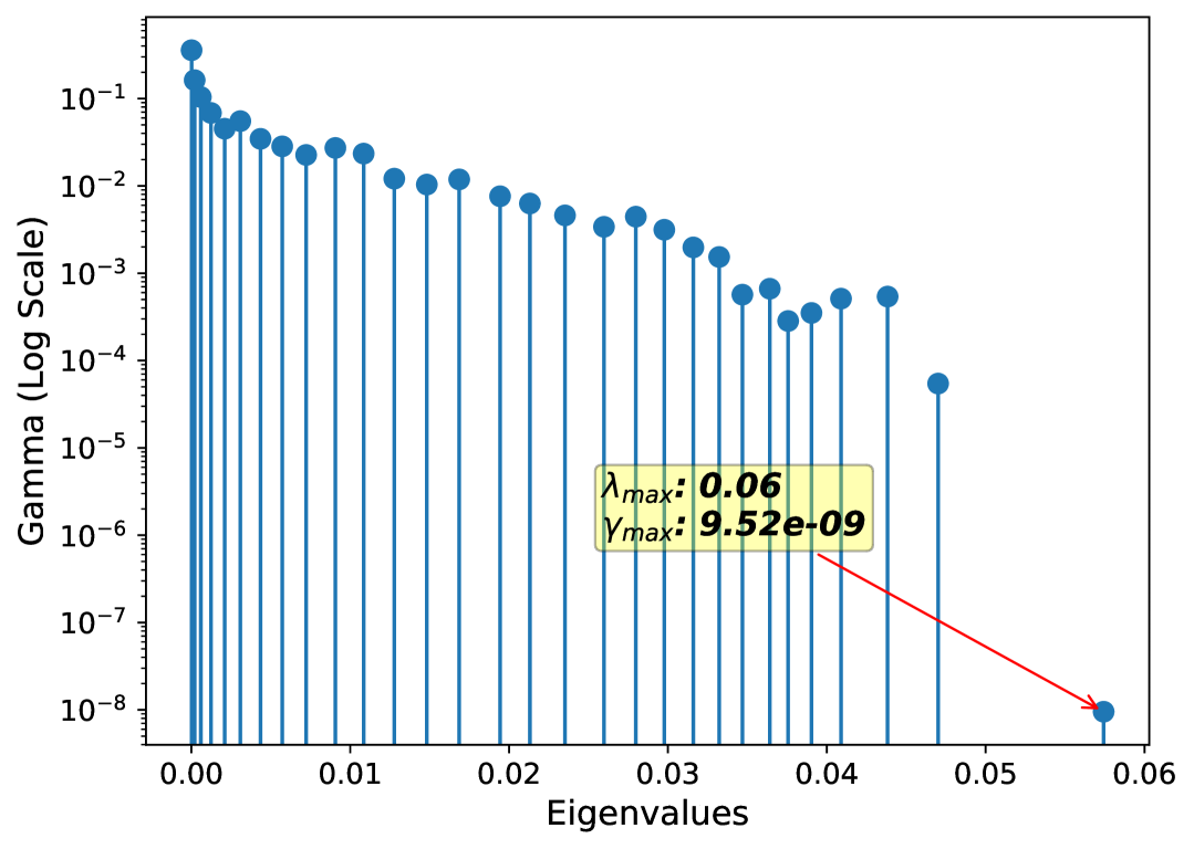
(j) $\alpha=1e{-5}$

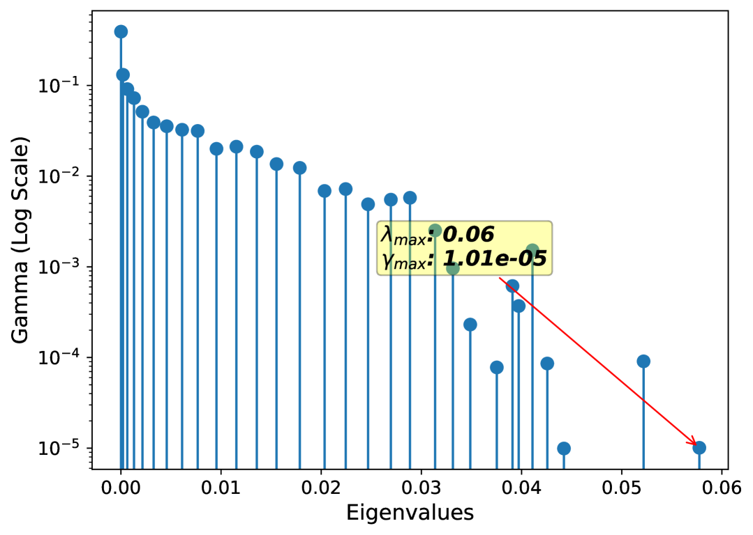
(k) $\alpha=0.0$

Figure 38: Hessian wrtx for learning rate 0.1

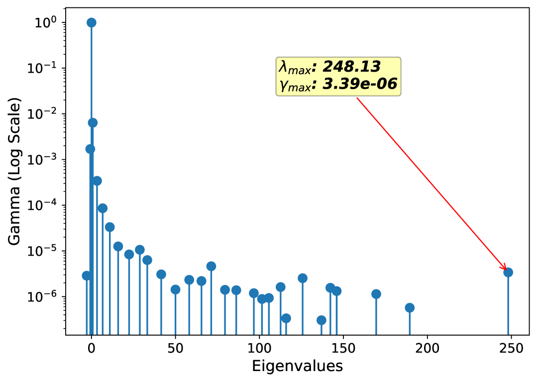
(a) $\alpha=0.3$

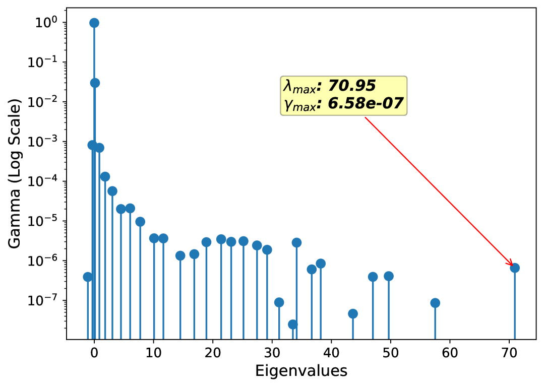
(b) $\alpha=0.1$

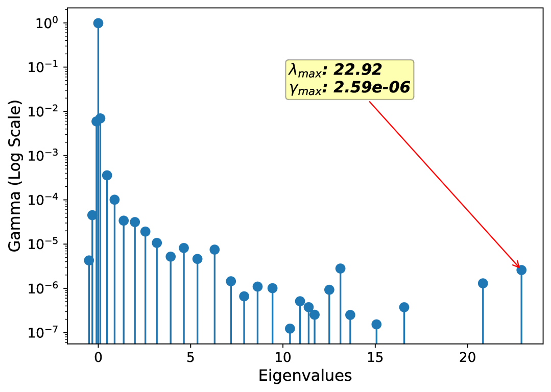
(c) $\alpha=0.03$

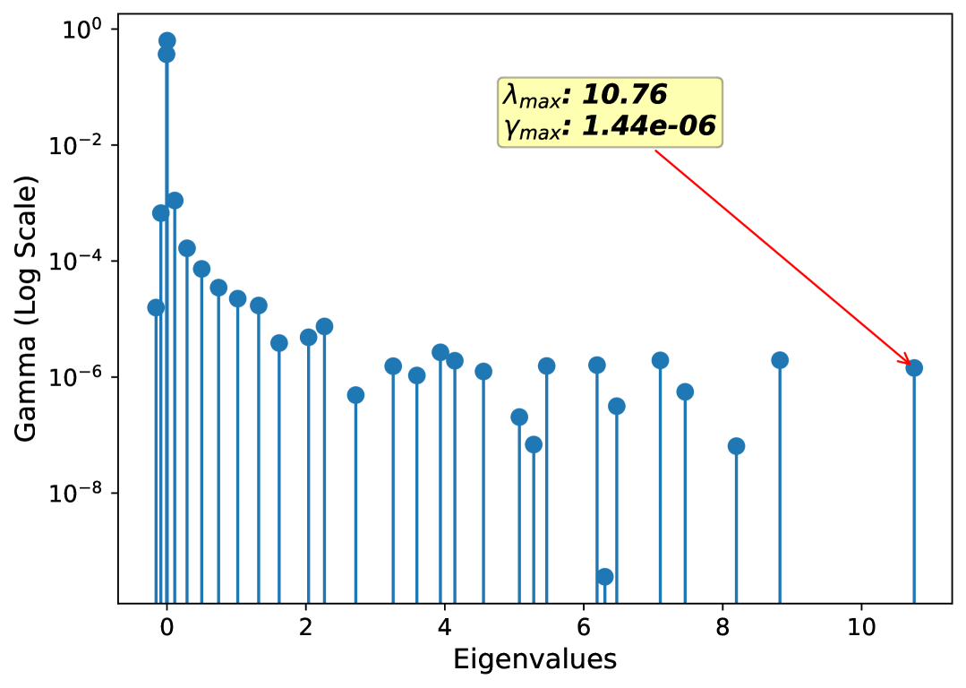
(d) $\alpha=0.01$

(e) $\alpha=0.003$

(f) $\alpha=0.001$

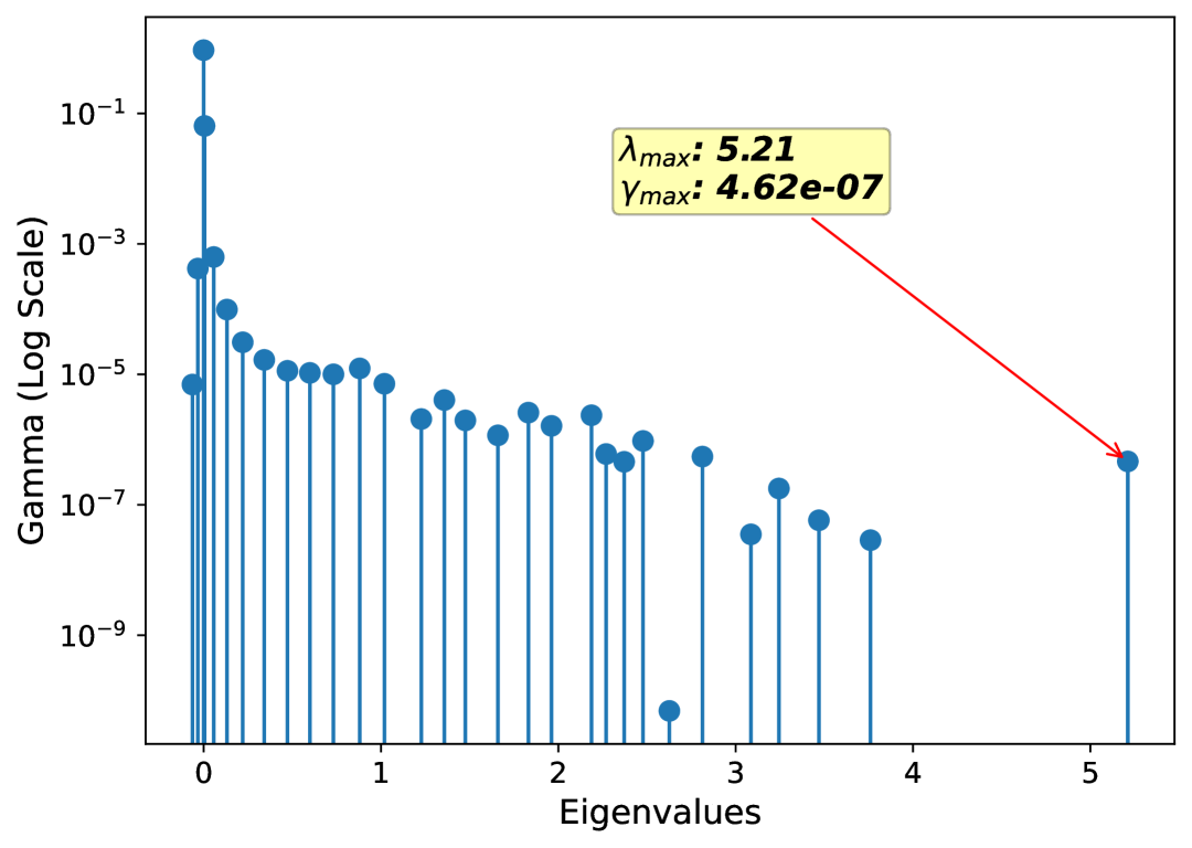
(g) $\alpha=0.0003$

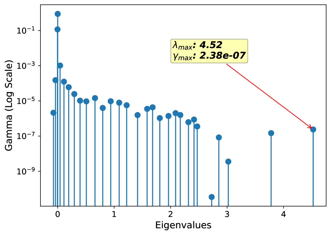
(h) $\alpha=0.0001$

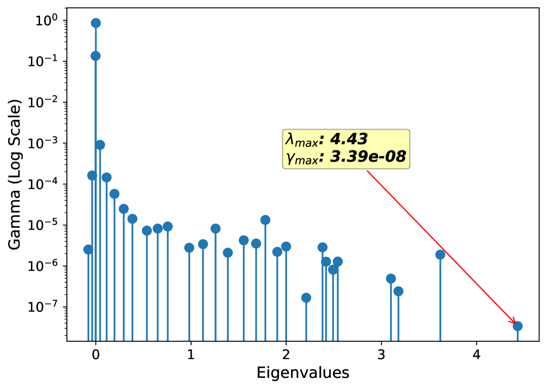
(i) $\alpha=3e{-5}$

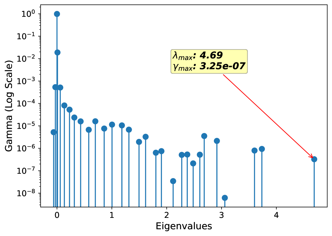
(j) $\alpha=1e{-5}$

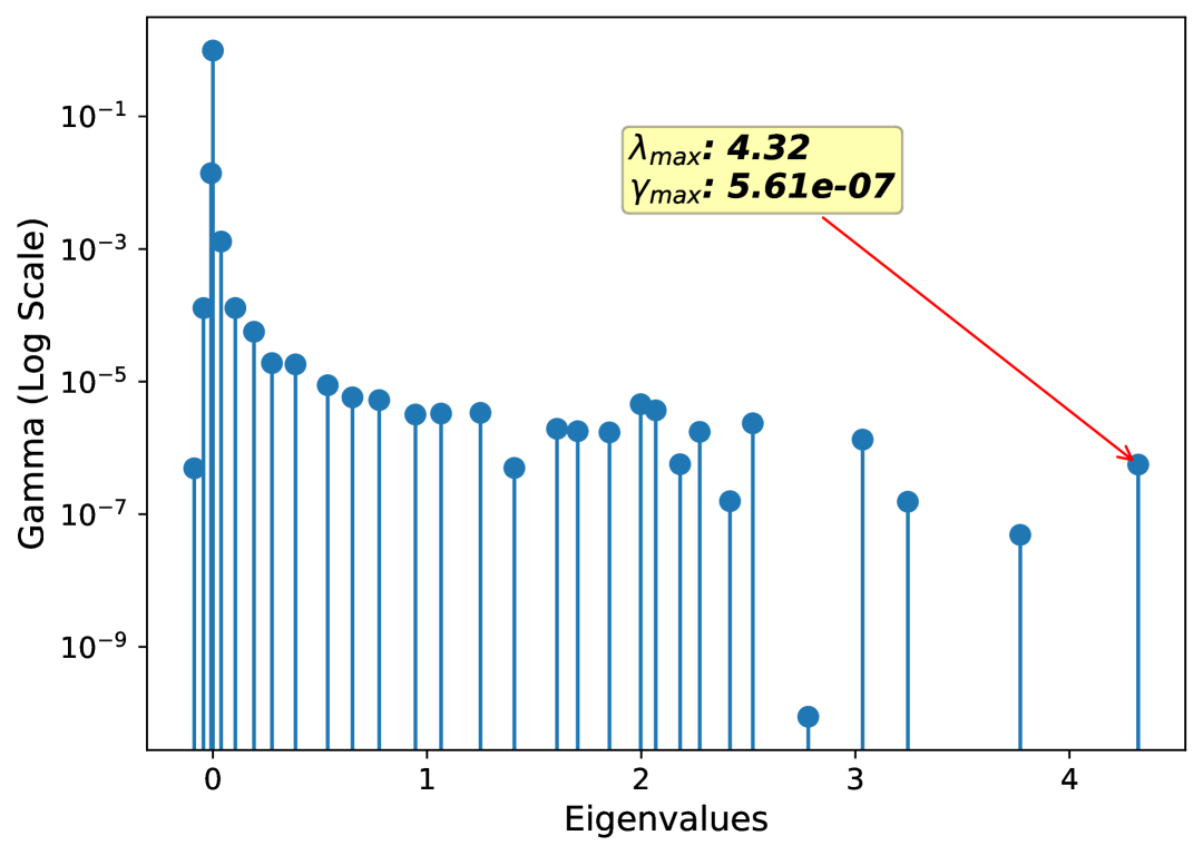
(k) $\alpha=0.0$

Figure 39: Hessian wrtw for learning rate 0.1

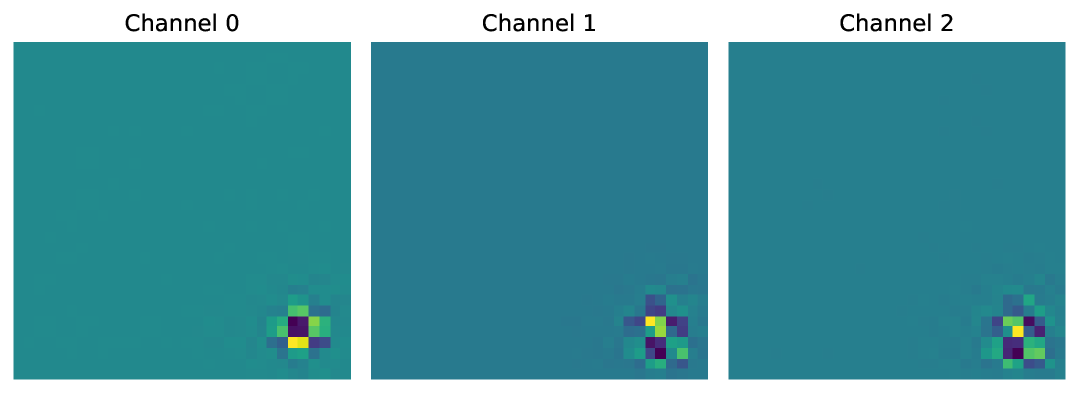
(a) $\alpha=0.3$

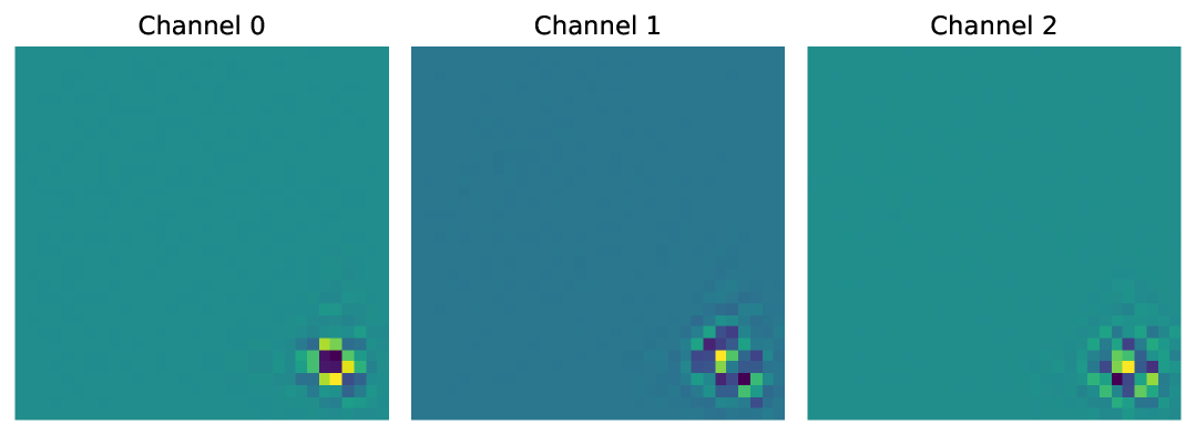
(b) $\alpha=0.1$

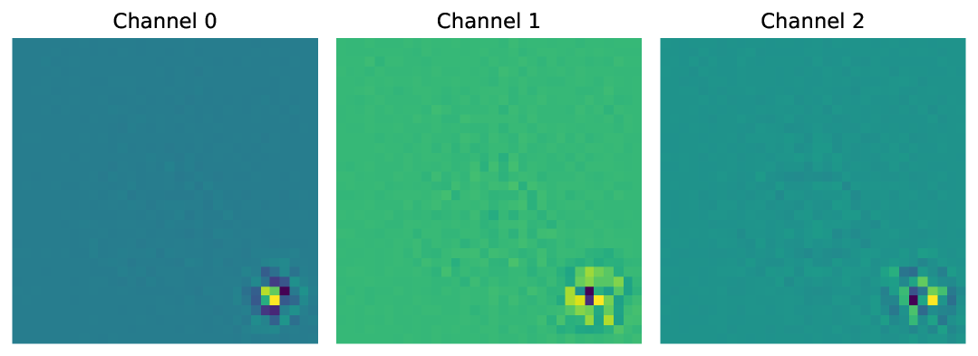
(c) $\alpha=0.03$

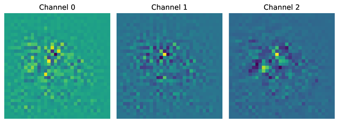
(d) $\alpha=0.01$

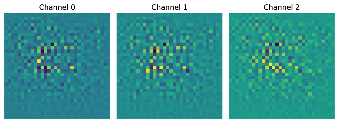
(e) $\alpha=0.003$

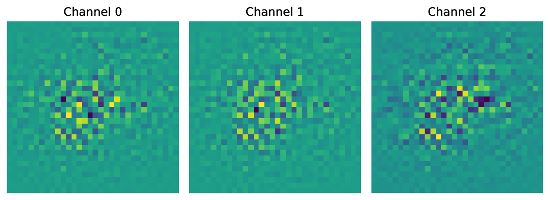
(f) $\alpha=0.001$

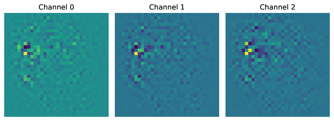
(g) $\alpha=0.0003$

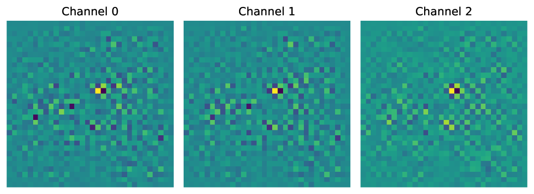
(h) $\alpha=0.0001$

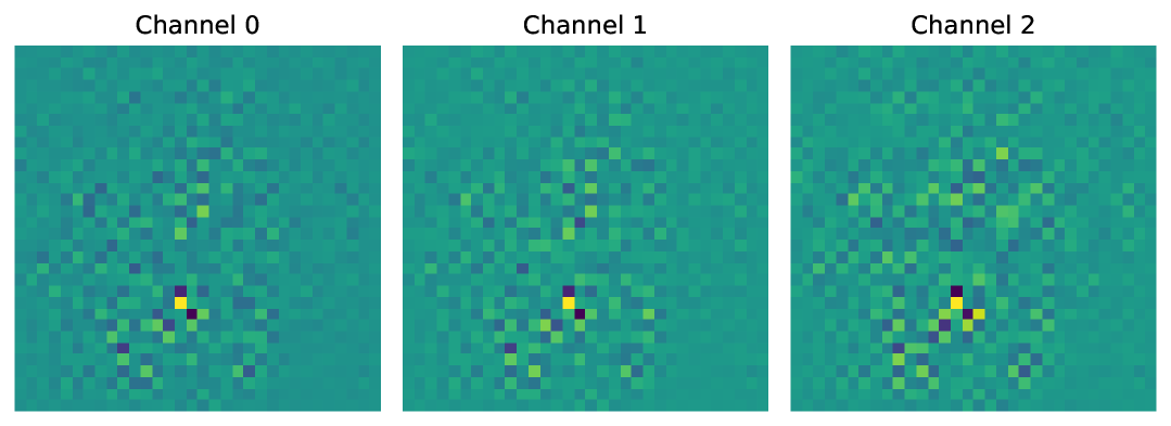
(i) $\alpha=3e{-5}$

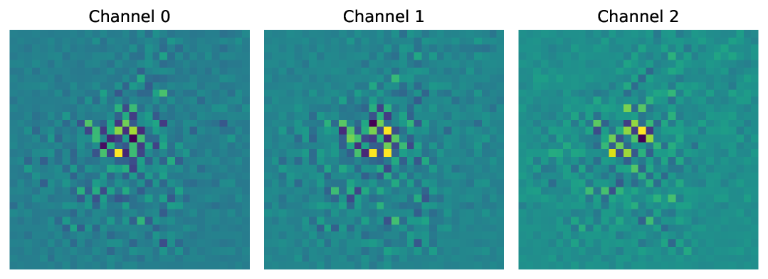
(j) $\alpha=1e{-5}$

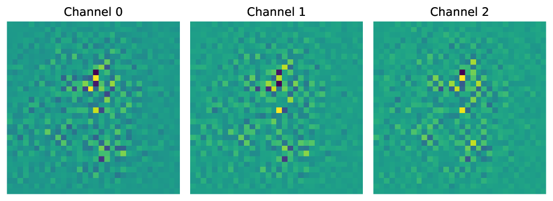
(k) $\alpha=0.0$

Figure 40: Top Eigenvalues for pos=29 and learning rate 0.1

References

- Benaych-Georges and Nadakuditi [2011] Florent Benaych-Georges and Raj Rao Nadakuditi. The eigenvalues and eigenvectors of finite, low rank perturbations of large random matrices. Advances in Mathematics, 227(1):494–521, 2011.
- Cai et al. [2022] Xiangrui Cai, Haidong Xu, Sihan Xu, Ying Zhang, and Xiaojie Yuan. BadPrompt: Backdoor attacks on continuous prompts. In Advances in Neural Information Processing Systems 35 (NeurIPS 2022), 2022.
- Carlini and Terzis [2022] Nicholas Carlini and Andreas Terzis. Poisoning and backdooring contrastive learning. In Proceedings of the International Conference on Learning Representations (ICLR), 2022. URL https://arxiv.org/abs/2106.09667.
- Carlini et al. [2019] Nicholas Carlini, Chang Liu, Úlfar Erlingsson, Jérôme Fernandez, and Dawn Song. The secret sharer: Measuring unintended neural network memorization & extracting secrets. In 28th USENIX Security Symposium (USENIX Security), pages 267–284, 2019.
- Chou et al. [2023] Sheng-Yen Chou, Pin-Yu Chen, and Tsung-Yi Ho. How to Backdoor Diffusion Models? In Proceedings of the IEEE/CVF Conference on Computer Vision and Pattern Recognition (CVPR), pages 4015–4024, 2023.
- Couillet and Liao [2022] Romain Couillet and Zhenyu Liao. Random matrix methods for machine learning. Cambridge University Press, 2022.
- Deng et al. [2009] Jia Deng, Wei Dong, Richard Socher, Li-Jia Li, Kai Li, and Li Fei-Fei. Imagenet: A large-scale hierarchical image database. In 2009 IEEE Conference on Computer Vision and Pattern Recognition, pages 248–255. IEEE, 2009.
- Gu et al. [2017] Tianyu Gu, Brendan Dolan-Gavitt, and Siddharth Garg. Badnets: Identifying vulnerabilities in the machine learning model supply chain, 2017.
- He et al. [2022] Hao He, Kaiwen Zha, and Dina Katabi. Indiscriminate poisoning attacks on unsupervised contrastive learning. arXiv preprint arXiv:2202.11202, 2022.
- Hong et al. [2022] Sanghyun Hong, Nicholas Carlini, and Alexey Kurakin. Handcrafted backdoors in deep neural networks. In Proceedings of the 36th Conference on Neural Information Processing Systems (NeurIPS), 2022. arXiv preprint arXiv:2106.04690.
- Hubinger et al. [2024] Evan Hubinger, Carson Denison, Jesse Mu, Mike Lambert, Meg Tong, Monte MacDiarmid, Tamera Lanham, Daniel M. Ziegler, Tim Maxwell, Newton Cheng, et al. Sleeper agents: Training deceptive LLMs that persist through safety training. arXiv preprint arXiv:2401.05566, 2024.
- Krizhevsky and Hinton [2009] Alex Krizhevsky and Geoffrey Hinton. Learning multiple layers of features from tiny images. Technical report, University of Toronto, 2009.
- LeCun et al. [1998] Yann LeCun, Léon Bottou, Yoshua Bengio, and Patrick Haffner. Gradient-based learning applied to document recognition. Proceedings of the IEEE, 86(11):2278–2324, 1998.
- Li et al. [2024] Yanzhou Li, Tianlin Li, Kangjie Chen, Jian Zhang, Shangqing Liu, Wenhan Wang, Tianwei Zhang, and Yang Liu. BadEdit: Backdooring large language models by model editing. In International Conference on Learning Representations (ICLR), 2024.
- Pan et al. [2024] Zhuoshi Pan, Yuguang Yao, Gaowen Liu, Bingquan Shen, H Vicky Zhao, Ramana Kompella, and Sijia Liu. From trojan horses to castle walls: Unveiling bilateral data poisoning effects in diffusion models. Advances in Neural Information Processing Systems, 37:82265–82295, 2024.
- Papernot et al. [2018] Nicolas Papernot, Patrick McDaniel, Arunesh Sinha, and Michael P Wellman. SoK: Security and privacy in machine learning. In 2018 IEEE European Symposium on Security and Privacy (EuroS&P), pages 399–414, 2018.
- Paszke et al. [2019] Adam Paszke, Sam Gross, Francisco Massa, Adam Lerer, James Bradbury, Gregory Chanan, Trevor Killeen, Zeming Lin, Natalia Gimelshein, Luca Antiga, Alban Desmaison, Andreas Köpf, Edward Yang, Zachary DeVito, Martin Raison, Alykhan Tejani, Sasank Chilamkurthy, Benoit Steiner, Lu Fang, Junjie Bai, and Soumith Chintala. Pytorch: An imperative style, high-performance deep learning library. In Advances in Neural Information Processing Systems, volume 32, pages 8024–8035, 2019.
- Radford et al. [2019] Alec Radford, Jeffrey Wu, Rewon Child, David Luan, Dario Amodei, and Ilya Sutskever. Language models are unsupervised multitask learners. OpenAI Blog, 1(8):1–24, 2019. Technical report.
- Radford et al. [2021] Alec Radford, Jong Wook Kim, Chris Hallacy, Aditya Ramesh, Gabriel Goh, Sandhini Agarwal, Girish Sastry, Amanda Askell, Pamela Mishkin, Jack Clark, Gretchen Krueger, and Ilya Sutskever. Learning transferable visual models from natural language supervision. In Proceedings of the 38th International Conference on Machine Learning (ICML), 2021.
- Shi et al. [2023] Jiawen Shi, Yixin Liu, Pan Zhou, and Lichao Sun. BadGPT: Exploring security vulnerabilities of ChatGPT via backdoor attacks to InstructGPT. arXiv preprint arXiv:2304.12298, 2023.
- Sun et al. [2020] Mengnan Sun, Shivangi Agarwal, and Zico Kolter. Poisoned classifiers are not only backdoored, they are fundamentally broken. arXiv preprint arXiv:2010.09080, 2020.
- Tao [2012] Terence Tao. Topics in random matrix theory. Graduate studies in mathematics ; v. 132. American Mathematical Society, Providence, R.I, 2012. ISBN 9780821874301.
- Touvron et al. [2023] Hugo Touvron, Thibaut Lavril, Gautier Izacard, Xavier Martinet, Marie-Anne Lachaux, Timothée Lacroix, Baptiste Rozière, Naman Goyal, Eric Hambro, Faisal Azhar, Armand Joulin, Edouard Grave, and Hervé Jegou. Llama: Open and efficient foundation language models. https://arxiv.org/abs/2302.13971, 2023. arXiv:2302.13971.
- Tran et al. [2018] Brandon Tran, Jerry Li, and Aleksander Madry. Spectral signatures in backdoor attacks. In Advances in Neural Information Processing Systems (NeurIPS), 2018.
- Wang et al. [2019] Bolun Wang, Yuanshun Yao, Shawn Shan, Huiying Li, Bimal Viswanath, Haitao Zheng, and Ben Y Zhao. Neural cleanse: Identifying and mitigating backdoor attacks in neural networks. In 2019 IEEE symposium on security and privacy (SP), pages 707–723. IEEE, 2019.
- Wang et al. [2024] Haonan Wang, Qianli Shen, Yao Tong, Yang Zhang, and Kenji Kawaguchi. The stronger the diffusion model, the easier the backdoor: Data poisoning to induce copyright breaches without adjusting finetuning pipeline. arXiv preprint arXiv:2401.04136, 2024.
- Wolf et al. [2020] Thomas Wolf, Lysandre Debut, Victor Sanh, Julien Chaumond, Clement Delangue, Anthony Moi, Pierric Cistac, Tim Rault, Rémi Louf, Morgan Funtowicz, Joe Davison, Sam Shleifer, Patrick von Platen, Clara Ma, Yacine Jernite, Julien Plu, Canwen Xu, Teven Le Scao, Sylvain Gugger, Mariama Drame, Quentin Lhoest, and Alexander M. Rush. Transformers: State-of-the-art natural language processing. In Proceedings of the 2020 Conference on Empirical Methods in Natural Language Processing: System Demonstrations, pages 38–45, Online, oct 2020. Association for Computational Linguistics. URL https://aclanthology.org/2020.emnlp-demos.6.
- Xiang et al. [2024] Zhen Xiang, Fengqing Jiang, Zidi Xiong, Bhaskar Ramasubramanian, Radha Poovendran, and Bo Li. BadChain: Backdoor chain-of-thought prompting for large language models. In International Conference on Learning Representations (ICLR), 2024.
- Xu et al. [2024] Yuancheng Xu, Jiarui Yao, Manli Shu, Yanchao Sun, Zichu Wu, Ning Yu, Tom Goldstein, and Furong Huang. Shadowcast: Stealthy data poisoning attacks against vision-language models. arXiv preprint arXiv:2402.06659, 2024.
- Zou et al. [2023] Andy Zou, Zifan Wang, Nicholas Carlini, Milad Nasr, J Zico Kolter, and Matt Fredrikson. Universal and transferable adversarial attacks on aligned language models. arXiv preprint arXiv:2307.15043, 2023.