Maximum Degree-Based Quasi-Clique Search via an Iterative Framework

Abstract.

Cohesive subgraph mining is a fundamental problem in graph theory with numerous real-world applications, such as social network analysis and protein-protein interaction modeling. Among various cohesive subgraphs, the $\gamma$-quasi-clique is widely studied for its flexibility in requiring each vertex to connect to at least a $\gamma$ proportion of other vertices in the subgraph. However, solving the maximum $\gamma$-quasi-clique problem is NP-hard and further complicated by the lack of the hereditary property, which makes designing efficient pruning strategies challenging. Existing algorithms, such as DDA and FastQC, either struggle with scalability or exhibit significant performance declines for small values of $\gamma$. In this paper, we propose a novel algorithm, IterQC, which reformulates the maximum $\gamma$-quasi-clique problem as a series of $k$-plex problems that possess the hereditary property. IterQC introduces a non-trivial iterative framework and incorporates two key optimization techniques: (1) the pseudo lower bound (pseudo LB) technique, which leverages information across iterations to improve the efficiency of branch-and-bound searches, and (2) the preprocessing technique that reduces problem size and unnecessary iterations. Extensive experiments demonstrate that IterQC achieves up to four orders of magnitude speedup and solves significantly more graph instances compared to state-of-the-art algorithms DDA and FastQC.

1. Introduction

Cohesive subgraph mining is a fundamental problem in graph theory with numerous real-world applications (Chang and Qin, 2018; Fang et al., 2020; Huang et al., 2019; Lee et al., 2010). Unlike cliques, which require complete connectivity, cohesive subgraphs provide more flexibility by allowing the absence of certain edges. In real-world graphs, data is often noisy and incomplete, making fully connected cliques impractical. By allowing a certain degree of edge absence, the relaxation offers a robust way to identify strongly connected substructures while accommodating missing or uncertain relationships. Various approaches have been proposed to relax the constraints of cohesive subgraph definitions, such as $k$-plex (Seidman and Foster, 1978), $k$-core (Seidman, 1983), and $k$-defective clique (Yu et al., 2006). One widely studied definition is the $\gamma$-quasi-clique (Matsuda et al., 1999). Given a fraction $\gamma$ between 0 and 1, a $\gamma$-quasi-clique requires that every vertex in the subgraph is directly connected to at least a $\gamma$ proportion of the other vertices in the subgraph. Cohesive subgraph mining in the context of $\gamma$-quasi-clique has recently attracted increasing interest (Zeng et al., 2007; Liu and Wong, 2008; Jiang and Pei, 2009; Pastukhov et al., 2018; Guo et al., 2020; Sanei-Mehri et al., 2021; Khalil et al., 2022; Yu and Long, 2023a). It has numerous applications in real-world graph structure analysis, including social network analysis (Bedi and Sharma, 2016; Guo et al., 2022; Fang et al., 2020) and the modeling of protein-protein interaction networks (Suratanee et al., 2014; Bader and Hogue, 2003; Bhattacharyya and Bandyopadhyay, 2009), which captures relationships between proteins. For example, in (Pei et al., 2005), researchers identify biologically significant functional groups by mining large $\gamma$-quasi-cliques that meet a minimum size threshold across various protein-protein and gene-gene interaction networks. The idea is that within a functional protein group, most members interact frequently, suggesting a high likelihood of forming a quasi-clique (Pei et al., 2005). Similarly, in another case study (Guo et al., 2022), $\gamma$-quasi-cliques are utilized to uncover meaningful communities within networks derived from publication data.

In this paper, we study the maximum $\gamma$-quasi-clique problem, which aims to identify the $\gamma$-quasi-clique with the largest number of vertices in a graph. As a natural extension of the classic maximum clique problem, this problem is unsurprisingly NP-hard (Matsuda et al., 1999; Pastukhov et al., 2018). An even more challenging lies in the fact that the $\gamma$-quasi-clique lacks the hereditary property, i.e., subgraphs of a $\gamma$-quasi-clique are not guaranteed to also be $\gamma$-quasi-cliques. This limitation complicates the design of efficient pruning methods, unlike problems for $k$-plex or $k$-defective clique, where the hereditary property enables effective optimizations. In this paper, we focus on designing practically efficient exact algorithms to tackle this challenging problem.

Existing state-of-the-art algorithms. The state-of-the-art algorithm for the maximum $\gamma$-quasi-clique problem is DDA (Pastukhov et al., 2018), which combines graph properties with techniques from operations research. A key feature of DDA is its iterative enumeration (or estimation) of the degree of the minimum-degree vertex in the maximum $\gamma$-quasi-clique. For each candidate degree, it invokes an integer programming (IP) solver multiple times to solve equivalent sub-problems and identify the final solution. Unlike other approaches relying solely on IP formulations or branch-and-bound techniques based on graph properties, DDA effectively integrates both. However, it has two limitations: (1) it naively enumerates possible minimum degree values, potentially requiring a large number of trials (e.g., DDA may enumerate $O(n)$ values, where $n$ is the number of vertices in the graph); (2) the IP solver operates as a black box, which makes it difficult to optimize for this specific problem.

Another closely related algorithm, FastQC (Yu and Long, 2023a), is the state-of-the-art for enumerating all maximal $\gamma$-quasi-cliques in a graph. FastQC uses a divide-and-conquer strategy with efficient pruning techniques that leverage intrinsic graph properties to systematically and effectively enumerate all maximal $\gamma$-quasi-cliques. It is clear that the largest maximal $\gamma$-quasi-clique identified corresponds to the maximum $\gamma$-quasi-clique. However, since FastQC is not specifically designed to solve the maximum $\gamma$-quasi-clique problem, even with additional pruning methods tailored for the maximum solution, its efficiency remains suboptimal. Moreover, our experimental results in Section 5 show that the efficiency of the FastQC algorithm significantly decreases when the value of $\gamma$ is relatively small.

In summary, while both DDA and FastQC have practical strengths, they fail to fully address the efficiency challenges of the maximum $\gamma$-quasi-clique problem. Their limitations in scalability and handling smaller values of $\gamma$ highlight the need for more specialized solutions.

Our new methods. In this work, we propose a novel algorithm, IterQC, which reformulates the maximum $\gamma$-quasi-clique problem as a series of $k$-plex problems. Notably, the $k$-plex possesses the hereditary property, enabling the design of more effective pruning methods. To achieve this, we introduce a non-trivial iterative framework that solves the maximum $\gamma$-quasi-clique problem through a carefully designed iterative procedure, leveraging repeated calls to a maximum $k$-plex solver (Wang et al., 2023; Chang and Yao, 2024; Gao et al., 2025). Building on this novel iterative framework, we further propose advanced optimization techniques, including the pseudo lower bound (pseudo LB) technique and the preprocessing technique. The pseudo LB technique effectively coordinates information between the inner iterations and the outer iterative framework, thereby boosting the overall efficiency of the iterative procedure. Meanwhile, the preprocessing technique performs preliminary operations before the iterative framework begins, reducing both the problem size by removing redundant vertices from the graph and reducing the number of iterations by skipping unnecessary iterations. With these optimizations, our proposed algorithm IterQC equipped with these optimizations achieves up to four orders of magnitude speedup and solves more instances compared to the state-of-the-art algorithms DDA and FastQC.

Contributions. Our main contributions are as follows.

• We first propose a basic iterative framework, which correctly transforms non-hereditary problems into multiple problem instances with the hereditary property. (Section 3)

• Based on the basic iterative method, we design an improved algorithm IterQC with two key components: (1) The pseudo lower bound (pseudo LB) technique, which utilizes information from previous iterations to generate a pseudo lower bound. This technique optimizes the branch-and-bound search, improving performance on challenging instances. (2) The preprocessing technique, which computes lower and upper bounds of the optimum size to remove unpromising vertices from the graph, potentially reducing the number of iterations. (Section 4)

• We conduct extensive experiments to compare IterQC with the state-of-the-art algorithms DDA and FastQC. The results show that (1) on the 10th DIMACS and real-world graph collections, the number of instances solved by IterQC within 3 seconds exceeds the number solved by the other two baselines within 3 hours; (2) on 30 representative graphs, IterQC is up to four orders of magnitude faster than the state-of-the-art algorithms. (Section 5)

2. Preliminaries

Let $G=(V,E)$ be an undirected simple graph with $|V|=n$ vertices and $|E|=m$ edges. We denote $G[S]$ of $G$ as the subgraph induced by the set of vertices $S$ of $V$. We use $d_{G}(v)$ to denote the degree of $v$ in $G$. Let $g$ be an induced subgraph of $G$. We denote the vertex set and the edge set of $g$ as $V(g)$ and $E(g)$, respectively. In this paper, we focus on the cohesive subgraph of $\gamma$-quasi-clique defined below.

Definition 0.

Given a graph $G=(V,E)$ and a real number $0<\gamma\leq 1$, an induced subgraph $g$ is said to be a $\gamma$-quasi-clique ($\gamma$-QC) if $\forall v\in V(g)$, $d_{g}(v)\geq\gamma\cdot(|V(g)|-1)$.

We are ready to present our problem in this paper.

Problem 1 (Maximum $\gamma$-quasi-clique).

Given a graph $G=(V,E)$ and a real number $\gamma\in[0.5,1]$, the Maximum $\gamma$-quasi-clique Problem (MaxQC) aims to find the largest $\gamma$-quasi-clique in $G$.

We first note that MaxQC has been proven to be NP-hard (Matsuda et al., 1999; Pastukhov et al., 2018). Moreover, we let $g^{*}$ be the largest $\gamma$-QC in $G$ and $s^{*}=|V(g^{*})|$ be the size of this maximum solution. We also note that, following previous studies (Guo et al., 2020; Khalil et al., 2022; Pei et al., 2005; Sanei-Mehri et al., 2021; Yu and Long, 2023a), we consider MaxQC with $\gamma\geq 0.5$ since (1) conceptually, a $\gamma$-QC with $\gamma<0.5$ may not be cohesive in practice (note that each vertex in such a $\gamma$-QC may connect to fewer than half of the other vertices); (2) technically, a $\gamma$-QC with $\gamma\geq 0.5$ has a small diameter of at most 2 (Pei et al., 2005).

3. Our Basic Iterative Framework

The design of efficient exact algorithms for MaxQC presents multiple challenges. First, MaxQC has been proven to be NP-hard (Matsuda et al., 1999; Pastukhov et al., 2018). Existing studies on similar maximum cohesive subgraph problems often adopt the branch-and-bound algorithmic framework (Chang et al., 2022; Chang and Yao, 2024; Wang et al., 2023). Second, the $\gamma$-quasi-clique is non-hereditary (Yu and Long, 2023a), i.e., an induced subgraph of a $\gamma$-QC is not necessarily a $\gamma$-QC. This non-hereditary property of the $\gamma$-QC complicates the design of effective bounding techniques within the branch-and-bound framework.

To address these challenges, our algorithm adopts an iterative framework that solves MaxQC by iteratively invoking a solver for another cohesive subgraph problem. The design rationale originates from the intention to convert the non-hereditary subgraph problem into multiple instances of a hereditary subgraph problem, so as to speed up the overall procedure.

We first introduce another useful cohesive subgraph structure.

Definition 0 ((Seidman and Foster, 1978)).

Given a graph $G=(V,E)$ and an integer $k\geq 1$, an induced subgraph $g$ is said to be a $k$-plex if $\forall v\in V(g)$, $d_{g}(v)\geq|V(g)|-k$.

In the literature, a related problem for $k$-plex is defined (Chang et al., 2022; Gao et al., 2018; Jiang et al., 2023, 2021; Wang et al., 2023; Xiao et al., 2017; Zhou et al., 2021; Balasundaram et al., 2011), as shown in the following.

Problem 2 (Maximum $k$-plex).

Given a graph $G=(V,E)$ and a positive integer $k$, the Maximum $k$-plex Problem aims to find the largest $k$-plex in $G$.

Based on the maximum $k$-plex problem, we next describe our basic iterative framework for the MaxQC problem. To simplify the description, we define the following two functions.

• get-k$(x):=\lfloor(1-\gamma)\cdot(x-1)\rfloor+1$, which takes a number $x$ of vertices as input and returns a appropriate value of $k$;

• solve-plex$(y):=\text{the size of the largest }y\text{-plex in }G$, which takes a value $y$ as input.

Input: A graph $G=(V,E)$ and a real value $0.5\leq\gamma\leq 1$

Output: The size of the maximum $\gamma$-quasi-clique in $G$

1 $s_{0}\leftarrow|V|$; $k_{1}\leftarrow\texttt{get-k}(s_{0})$; $i\leftarrow 1$;

2 while true do

3    $s_{i}\leftarrow$ solve-plex($k_{i}$);

4    if $k_{i}=\emph{{get-k}}(s_{i})$ then

5       $s^{*}\leftarrow s_{i}$; return $s^{*}$;

6      

7   $k_{i+1}\leftarrow\texttt{get-k}(s_{i})$; $i\leftarrow i+1$;

8   

Algorithm 1 A Basic Iterative Framework

We present our basic iterative framework for solving MaxQC in Algorithm 1. Specifically, Algorithm 1 initializes $s_{0}$ as the number of vertices in the graph $G$, computes the corresponding value of $k_{1}$ using the function get-k, and sets the index $i$ as 1 (Line 1). The algorithm then iteratively computes $s_{i}$ by solving the maximum $k_{i}$-plex problem via the function solve-plex, while updating $k_{i}$ via the function get-k in each iteration (Lines 2-6). The iteration terminates when $k_{i}=\texttt{get-k}(s_{i})$ in Line 4, at which point $s^{*}$, the size of the maximum $\gamma$-quasi-clique, is returned in Line 5. Note that Algorithm 1 returns only the size of the maximum $\gamma$-quasi-clique, but can be easily modified to output the corresponding subgraph.

Correctness. We now prove the correctness of our basic iterative framework in Algorithm 1. For simplicity in the proof, we assume that the termination condition (Line 4) of Algorithm 1 is met at the $(p+1)$-st iteration. Then, in our iterative framework, we can obtain two sequences $\{s_{0},s_{1},\ldots,s_{p},s_{p+1}\}$ and $\{k_{1},k_{2},\ldots,k_{p},k_{p+1}\}$, where $k_{p+1}=\texttt{get-k}(s_{p+1})$. In our proof, we will show that the sequence of $\{s_{0},s_{1},\ldots,s_{p}\}$ generated by Algorithm 1 is strictly decreasing and $s_{p+1}$ corresponds to the largest $\gamma$-quasi-clique in the graph, i.e, $s_{p+1}=s^{*}$. We first consider the special case that the input graph $G$ is already a $\gamma$-quasi-clique.

Lemma 0.

When the input graph $G=(V,E)$ is a $\gamma$-QC, Algorithm 1 correctly returns $|V|$ as the optimum solution.

The proof of Lemma 3.2, along with other omitted proofs in this section, can be found in Section A.1. In the following, we discuss the correctness of the algorithm where $G$ itself is not a $\gamma$-quasi-clique. We first prove the properties of the sequence for $s$ in the following.

Lemma 0.

For the sequence $\{s_{0},s_{1},\ldots,s_{p}\}$, two consecutive elements are not identical, i.e., $\forall 0\leq i\leq p-1$, $s_{i}\neq s_{i+1}$.

Lemma 0.

The sequence $\{s_{0},s_{1},\ldots,s_{p}\}$ is strictly decreasing.

Proof.

We prove this lemma by the mathematical induction.
\scriptsize{1}⃝ $p=1$. As we consider the case where $G$ itself is not a $\gamma$-quasi-clique (by Lemma 3.2), we have $s_{p}=s_{1}=\texttt{solve-plex}(k_{1})<s_{0}$. The base case holds true.
\scriptsize{2}⃝ $p\geq 2$. Assume that the induction holds for $p-1$, i.e., we have $s_{p-1}<s_{p-2}$. We observe that get-k is a non-decreasing function, which implies that $\texttt{get-k}(s_{p-1})\leq\texttt{get-k}(s_{p-2})$. Moreover, by the definition of the solve-plex function, for any $y_{1}>y_{2}$, the inequality $\texttt{solve-plex}(y_{1})\geq\texttt{solve-plex}(y_{2})$ holds. Then we have

$$s_{p} =\texttt{solve-plex}(k_{p})=\texttt{solve-plex}(\texttt{get-k}(s_{p-1}))$$

$$\leq\texttt{solve-plex}(\texttt{get-k}(s_{p-2}))=\texttt{solve-plex}(k_{p-1})=s_{p-1}.$$

Note that based on Lemma 3.3 the sequence $\{s_{0},s_{1},\ldots,s_{p}\}$ ensures that no two adjacent elements share the same value, which implies $s_{p}<s_{p-1}$, completing the inductive step.

Based on \scriptsize{1}⃝, \scriptsize{2}⃝, and the principle of mathematical induction, we complete the proof of Lemma 3.4. ∎

Based on Lemma 3.4, we can obtain the following corollary.

Corollary 0.

The sequence $\{s_{0},s_{1},\ldots,s_{p}\}$ is finite.

We then show the relationship between $\{s_{0},s_{1},\ldots,s_{p},s_{p+1}\}$ and the size of the largest $\gamma$-quasi-clique.

Lemma 0.

$\forall s_{i}\in\{s_{0},s_{1},\ldots,s_{p+1}\},\,s_{i}\geq s^{*}$ holds.

Lemma 0.

Algorithm 1 correctly identifies the largest $\gamma$-quasi-clique, i.e., $s_{p+1}=s^{*}$.

Proof.

We prove by contradiction. By Lemma 3.6, we assume, to the contrary, that $s_{p+1}>s^{*}$. According to the termination condition in Line 4 of Algorithm 1, we have $k_{p+1}=\texttt{get-k}(s_{p+1})=1+\lfloor(1-\gamma)\cdot(s_{p+1}-1)\rfloor$. Thus, it is clear that the result obtained by $\texttt{solve-plex}(k_{p+1})$ is a $\gamma$-quasi-clique of size $s_{p+1}$, which contradicts $s^{*}$ being the size of the maximum $\gamma$-quasi-clique. ∎

Discussions. We first note that an example of Algorithm 1 and its iterative process are provided in Appendix B. As shown in Lemma 3.7, Algorithm 1 can correctly solve MaxQC. The time complexity analysis is simple, since there are at most $n$ iterations (Lines 2-6) and each iteration invokes a solver for the maximum $k$-plex problem. Note that the current best time complexities of the maximum $k$-plex algorithms are $O^{*}((k+1)^{\delta+k-s^{*}})$ and $O^{*}(\gamma_{k}^{\delta})$ (Wang et al., 2023; Chang and Yao, 2024; Gao et al., 2025), where ${O^{*}}$ suppresses the polynomial factors, $\gamma_{k}<2$ is the largest real root of $x^{k+3}-2x^{k+2}+x^{2}-x+1=0$, and $\delta$ is the degeneracy of the graph. We also remark that prior studies adopted similar approaches by reducing a more difficult problem to solving another problem iteratively. For instance, Chang and Yao (Chang and Yao, 2024) briefly discuss the relationship between the $\gamma$-quasi-clique and the $k$-plex. They focus on enumerating maximal $\gamma$-quasi-cliques and mention a method for generating an initial solution set by enumerating maximal $k$-plexes, followed by a screening step to remove those that do not satisfy the maximality condition. However, this method is mainly of theoretical interest and runs slowly in practice, since it requires enumerating a large number of maximal $k$-plexes. Zhang and Liu (Zhang and Liu, 2023) tackle the minimum $k$-core problem by reducing it to multiple iterations of solving the maximum $k$-plex problem. Their iterative strategy incrementally adjusts the value of $k$ by one in each round, progressively approaching the desired solution. Similarly, they also adopt an iterative strategy that considers different values of $k$, where the value of $k$ differs by one between consecutive iterations. In contrast, we consider the maximum $\gamma$-quasi-clique problem. Our method adaptively adjusts the values of $k$ based on the size of the current best $k$-plex, rather than exhaustively enumerating all possible values of $k$.

However, Algorithm 1 still suffers from efficiency issues for the following reasons. First, Algorithm 1 utilizes a solver for solve-plex as a black box. This solver relies on a conservative lower bound within solve-plex to reduce the graph, leading to inefficiencies when handling certain challenging instances. Second, the graph processed iteratively in solve-plex (Line 3) often contains many unpromising vertices, which negatively affects overall performance, even after graph reduction within solve-plex. Further, in the initial iteration, the first value of $k$ is set as $k_{1}=\texttt{get-k}(|V|)$ with $|V|$ is a trivial upper bound of $s^{*}$ in Line 1. This initialization could potentially result in numerous unnecessary iterations of Lines 2-6.

4. Our Improved Algorithm: IterQC

To address the limitations of our basic iterative framework (Algorithm 1), we propose an advanced iterative method IterQC (shown in Algorithm 2), which incorporates two key stages: the preprocessing stage and the iterative search stage. First, we consider the iterative search stage (Line 4). Within the function Plex-Search – an improved version of solve-plex from Algorithm 1 – we introduce a pseudo lower bound (pseudo LB). This technique improves practical performance when handling challenging instances while preserving the correctness of the iterative algorithm for MaxQC. The pseudo LB technique is discussed in Section 4.1. Second, we provide a preprocessing technique (Lines 1-3) to improve efficiency. Specifically, we compute both the lower and upper bounds, $lb$ and $ub$, of the size $s^{*}$ of the largest $\gamma$-quasi-clique $g^{*}$ via Get-Bounds in Line 1. Using $lb$ and $ub$, in Lines 2-3, we can (1) reduce the graph by removing unpromising vertices/edges from $G$ that cannot appear in $g^{*}$, and (2) initialize a smaller value of $k$ for Plex-Search, potentially reducing the number of iterations. The preprocessing technique is introduced in Section 4.2. Finally, we analyze the time complexity of our IterQC, which theoretically improves upon the state-of-the-art algorithms, in Section 4.3

Input: A graph $G=(V,E)$ and a real value $0.5\leq\gamma\leq 1$

Output: The size of the maximum $\gamma$-quasi-clique in $G$

// Stage 1: Preprocessing

1 $lb,ub\leftarrow\texttt{Get-Bounds}(G,\gamma)$ ;

2

3while $\min_{v\in V}d_{G}(v)\leq\lfloor(lb-1)\cdot\gamma\rfloor$ do

4    $u\leftarrow\arg\min_{v\in V}d_{G}(v)$; Remove $u$ from $G$;

5   

// Stage 2: Iterative Search

6 Improved-Iter-Search$(G,\gamma,ub)$;

Algorithm 2 Our Improved Algorithm: IterQC

4.1. A Novel Pseudo Lower Bound Technique

The basic iterative framework (Algorithm 1) solves MaxQC by iteratively invoking the maximum $k$-plex solver solve-plex as a black box with varying values of $k$. To improve practical efficiency, we have the following key observation.

Key observation. Existing studies (Xiao et al., 2017; Chang et al., 2022; Jiang et al., 2023; Wang et al., 2023; Chang and Yao, 2024; Gao et al., 2025) on maximum $k$-plex solvers mainly consist of two steps: (1) heuristically computing a lower bound of the maximum $k$-plex, and (2) exhaustively conducting a branch-and-bound search to find the final result. It is well known that Step (1) has a polynomial complexity while Step (2) requires an exponential complexity. Thus, both theoretically and practically, in most cases, the time cost of the branch-and-bound search dominates that of obtaining the lower bound.

With the above property, our key idea is to balance the time cost of both steps. In particular, we introduce a pseudo lower bound, denoted by $pseudo\mbox{-}lb$, which is defined as the average of the heuristic lower bound from Step (1) and a known upper bound for the maximum $k$-plex solution. In other words, $pseudo\mbox{-}lb$ is always at least the heuristic lower bound and at most the known upper bound. By incorporating $pseudo\mbox{-}lb$ into the branch-and-bound search in Step (2), we may improve pruning effectiveness, which reduces the overall search time as verified by our experiments. We note that in maximum $k$-plex algorithms, Step (1) corresponds to Plex-Heu for computing a heuristic solution, while Step (2) corresponds to Plex-BRB for performing the branch-and-bound search.

The technique of pseudo LB. We call this technique as pseudo lower bound (pseudo LB), which is incorporated into a branch-and-bound search algorithm called Plex-Search in Algorithm 3. In Plex-Search, $ub\mbox{-}plex$ represents an upper bound of the size of the maximum $k$-plex found in Plex-Search, meaning no $k$-plex larger than $ub\mbox{-}plex$ exists. The output of Plex-Search include a pseudo lower bound $pseudo\mbox{-}lb$ and a pseudo size $|S|$ which corresponds to (1) the size of the maximum $k$-plex of size at least $pseudo\mbox{-}lb$ if such a $k$-plex exists, or (2) 0, if no $k$-plex of size at least $pseudo\mbox{-}lb$ exists. This is because, when the input $pseudo\mbox{-}lb$ exceeds the size of the maximum $k$-plex in the graph, Plex-BRB will utilize this $pseudo\mbox{-}lb$ for pruning, resulting in an empty graph as the vertex set $S$.

Our Plex-Search method. We describe Plex-Search in Algorithm 3. Specifically, in Line 1, we invoke Plex-Heu to compute a lower bound $lb\mbox{-}plex$. If $lb\mbox{-}plex=ub\mbox{-}plex$, we can directly return $lb\mbox{-}plex$ as both the pseudo lower bound and the pseudo size in Line 2, since Plex-Heu already finds the maximum $k$-plex in this case. Then, Line 3 computes our pseudo lower bound $pseudo\mbox{-}lb$ as the average of $lb\mbox{-}plex$ and $ub\mbox{-}plex$. We conduct Plex-BRB using $pseudo\mbox{-}lb$ for pruning and obtain the corresponding $k$-plex $S$ (either the vertex set of maximum $k$-plex or an empty set). Finally, we return $pseudo\mbox{-}lb$ and $|S|$ in Line 5.

Output: a pseudo lower bound $pseudo\mbox{-}lb$ and a pseudo size

$lb\mbox{-}plex\leftarrow\texttt{Plex-Heu}(G)$; // $G$ is locally reduced.

1 if $lb\mbox{-}plex=ub\mbox{-}plex$ then  return $lb\mbox{-}plex,lb\mbox{-}plex$;

2 $pseudo\mbox{-}lb\leftarrow\lfloor(lb\mbox{-}plex+ub\mbox{-}plex)/2\rfloor$;

$S\leftarrow\texttt{Plex-BRB}(G,pseudo\mbox{-}lb)$; // The maximum $k$-plex of size at least $pseudo\mbox{-}lb$ if exists; empty, otherwise.

3 return $pseudo\mbox{-}lb,|S|$;

Algorithm 3 Plex-Search$(G,k,ub\mbox{-}plex)$

Our improved iterative search algorithm. With our newly proposed Plex-Search with the pseudo LB technique, we next present our improved iterative search method Improved-Iter-Search in Algorithm 4. This method is similar to our basic iterative framework in Algorithm 1. Specifically, Algorithm 4 initializes $s_{0}$ to $ub$, computes the corresponding value of $k_{1}$ using the function get-k, and sets the index $i$ to 1 (Line 1). The algorithm then iteratively computes $s_{i}$ by invoking Plex-Search (instead of solve-plex in Algorithm 1), while updating $k_{i}$ using the function get-k at each iteration (Lines 2-6). Note that both $pseudo\mbox{-}lb$ and $pseudo\mbox{-}size$ are obtained from our Plex-Search, and $s_{i}$ is set to the greater of these two values in Line 3. The iteration terminates when $k_{i}=\texttt{get-k}(s_{i})$ and $pseudo\mbox{-}size\geq pseudo\mbox{-}lb$ in Line 4. This termination condition ensures that (1) the output from Plex-Search is the maximum $k$-plex even with the use of a pseudo lower bound; and (2) the current iteration produces the same value of $k$ for the next iteration from Plex-Search. At this point, we return $s^{*}$ as the size of the maximum $\gamma$-quasi-clique in Line 5.

Output: The size of the maximum $\gamma$-quasi-clique in $G$

1 $s_{0}\leftarrow ub$; $k_{1}\leftarrow\texttt{get-k}(s_{0})$; $i\leftarrow 1$;

2 while true do

3    $pseudo\mbox{-}lb,pseudo\mbox{-}size\leftarrow$ Plex-Search($G$, $k_{i}$, $s_{i-1}$); $s_{i}\leftarrow\max\{pseudo\mbox{-}lb,pseudo\mbox{-}size\}$;

4    if $k_{i}=\emph{{get-k}}(s_{i})$ and $pseudo\mbox{-}size\geq pseudo\mbox{-}lb$ then

5       $s^{*}\leftarrow s_{i}$; return $s^{*}$;

6      

7   $k_{i+1}\leftarrow\texttt{get-k}(s_{i})$; $i\leftarrow i+1$;

8   

Algorithm 4 Improved-Iter-Search$(G,\gamma,ub)$

Remark. We note that our improved iterative search method in Algorithm 4 can use adaptions of any existing maximum $k$-plex algorithm (Xiao et al., 2017; Chang et al., 2022; Jiang et al., 2023; Wang et al., 2023; Chang and Yao, 2024; Gao et al., 2025) for Plex-Search, provided the algorithm can be decomposed into two steps: (1) heuristically obtaining a lower bound for the maximum $k$-plex, Plex-Heu, and (2) exhaustively conducting the exact branch-and-bound search for the final solution, Plex-BRB. In this work, we utilize one of the state-of-the-art maximum $k$-plex algorithms KPEX (Gao et al., 2025).

Correctness. We prove the correctness of our improved iterative search algorithm Improved-Iterative-Search in Algorithm 4, which includes the pseudo LB technique in Algorithm 3. The complete proof and the illustration example of the pseudo LB technique are provided in Appendix A.2 and Appendix B, respectively.

4.2. Our Preprocessing Technique

To show our preprocessing technique, we first describe the computation of lower and upper bounds Get-Bounds (Line 1 of Algorithm 2).

Computation of lower and upper bounds. Following the idea commonly adopted for computing lower and upper bounds in prior dense subgraph search studies (Yu and Long, 2023a; Chang et al., 2022; Chang, 2023; Rahman et al., 2024), we derive our bounds based on the $k$-core structure. In the following, we introduce the relevant concepts and present the bounds for our problem.

Definition 0.

($k$-core (Seidman, 1983)) Given a graph $G$ and an integer $k$, the $k$-core of $G$ is the maximal subgraph $g$ of $G$ such that every vertex $u\in V(g)$ has degree $d_{g}(u)\geq k$ in $g$.

Based on the $k$-core, a related concept is the core number of a vertex $u$, denoted as ${core}(u)$, which is the largest $k$ such that $u$ is part of a $k$-core in the graph. In other words, $u$ cannot belong to any subgraph where all vertices have a degree of at least $core(u)+1$. Let $max\_core$ be the maximum core number in the graph, i.e., $max\_core=\max_{u\in V}core(u)$. Given a graph $G=(V,E)$, the core numbers for all vertices can be computed in $O(|V|+|E|)$ time using the famous peeling algorithm (Matula and Beck, 1983; Batagelj and Zaveršnik, 2003), which iteratively removes vertices with the smallest degree from the current graph. We remark that during the peeling algorithm used to compute the core numbers, we can obtain the lower bound $lb$ of $s^{*}$ as a by-product. In particular, we check whether the current graph qualifies as a $\gamma$-quasi clique and record the size of the largest qualifying $\gamma$-quasi clique. Moreover, as the current graph keeps shrinking during the peeling algorithm, the lower bound $lb$ clearly corresponds to the size of the first current graph that meets the $\gamma$-quasi clique requirements.

Lemma 0.

Given a graph $G$ and a real number $0<\gamma\leq 1$, we have $s^{*}\leq 1+\lceil max\_core/\gamma\rceil$.

The proof of Lemma 4.2 directly follows from the fact that the minimum degree of a $\gamma$-QC is at most $max\_core$ and the definition of $\gamma$-QC.

Output: The lower and upper bounds $lb$ and $ub$ of $s^{*}$

1

2$lb\leftarrow 0$; $ub\leftarrow 0$; $max\_core\leftarrow 0$;

3

4while $V(G)\neq\emptyset$ do

5    $u\leftarrow\arg\min_{v\in V(G)}d_{G}(v)$;

6    $max\_core\leftarrow\max(max\_core,d_{G}(u))$;

7    $ub\leftarrow\max(ub,\min(1+\lceil max\_core/\gamma\rceil,|V(G)|))$;

8    if $G$ is a $\gamma$-quasi-clique and $lb=0$ then

9       $lb\leftarrow|V(G)|$;

10      

11   Remove $u$ from $G$;

12   

13return $lb$, $ub$;

Algorithm 5 Get-Bounds$(G,\gamma)$

Our method Get-Bounds for computing both lower and upper bounds is summarized in Algorithm 5. In particular, as mentioned, Algorithm 5 follows the peeling algorithm, which iteratively removes the vertex with the smallest degree from the current graph while dynamically updating $ub$ and $lb$.

The preprocessing stage. After obtaining both lower and upper bounds via Get-Bounds, we show how to utilize these bounds in our preprocessing. Recall that, with $lb$ and $ub$, we can (1) reduce the graph by removing unpromising vertices from $G$ that cannot appear in $g^{*}$ using $lb$, and (2) set a smaller initial value of $k$ in the function Plex-Search using $ub$. The details are as follows. For (1), we can iteratively remove vertices from $G$ with degrees at most $\lfloor(lb-1)\cdot\gamma\rfloor$ and their incident edges, since it is clear that no solution of size greater than $lb$ can still include these vertices. For (2), we can easily derive from Lemma A.1 (Section 4 where the proofs are in Appendix A.2) that, instead of initializing $s_{0}$ as $|V|$, $s_{0}$ can be set to an integer larger than $s^{*}$ while still ensuring our iterative framework produces the correct solution. This allows us to use the obtained upper bound $ub$ to update $s_{0}$. Additionally, this $ub$ is used to generate the initial value of $k$ for Plex-Search through get-k, while maintaining the correctness of the iterative framework.

4.3. Time Complexity Analysis

As mentioned, in our implementation of Improved-Iter-Search (or specifically, Plex-Solve in Algorithm 3), we use two components, i.e., the heuristic and the branch-and-bound search, of the maximum $k$-plex solver kPEX (Gao et al., 2025). The time complexity of our exact algorithm IterQC is dominated by Plex-BRB in Algorithm 3, which is invoked at most $n$ times. The time complexities of kPEX are $O^{*}((k+1)^{\delta+k-s^{*}})$ and $O^{*}(\gamma_{k}^{\delta})$, where ${O^{*}}$ suppresses the polynomials, $\gamma_{k}<2$ is the largest real root of $x^{k+3}-2x^{k+2}+x^{2}-x+1=0$, and $\delta$ is the degeneracy of the graph. These complexities are derived using the branching methods in (Wang et al., 2023; Chang and Yao, 2024), which represent the current best time complexities for the maximum $k$-plex problem. In addition, as the sequence $\{s_{1},s_{2},\ldots,s_{p}\}$ generated by our improved iterative framework is monotonically decreasing and get-k is a non-decreasing function, each value of $k_{i}$ is thus upper bounded by $k_{1}$. Thus, the time complexity of each iteration depends on solving the maximum $k$-plex problem with $k_{1}$. Further, with the preprocessing technique, $k_{1}=\delta\frac{1-\gamma}{\gamma}$ and we let $k=k_{1}$. Therefore, the time complexity of IterQC is given by $O^{*}\left(\min\left\{\left(\delta+1\right)^{2\delta-s^{*}},\gamma_{k}^{\delta}\right\}\right).$ This improves upon (1) the time complexity of FastQC (Yu and Long, 2023a), which is $O^{*}(\sigma_{k}^{\delta\cdot\Delta})$, where $\Delta$ denotes the maximum degree of vertices in the graph and $\gamma_{k}<\sigma_{k}$ for each $k$, and improves upon (2) the time complexity of DDA (Pastukhov et al., 2018), which is $O^{*}(2^{n})$.

5. Experiments

We conduct extensive experiments to evaluate the practical performance of our exact algorithm IterQC against other exact methods.

• DDA: the state-of-the-art algorithm (Pastukhov et al., 2018).

• FastQC: a baseline adapted from the state-of-the-art algorithm for enumerating all maximal $\gamma$-QCs of size at least a given lower bound (Yu and Long, 2023a). We adapt FastQC for our MaxQC problem by tracking of the largest maximal $\gamma$-QC seen so far and dynamically updating the lower bound to facilitate better pruning. Note that the largest $\gamma$-QC is the largest one among all maximal $\gamma$-QCs.

Setup. All algorithms are implemented in C++, compiled with g++ -O3, and run on a machine with an Intel CPU @ 2.60GHz and 256GB main memory running Ubuntu 20.04.6. We set the time limit as 3 hours (i.e., 10,800s) and use OOT (Out Of Time limit) to represent the time exceeds the limit. Our source code can be found at https://github.com/SmartProbiotics/IterQC.

Datasets. We evaluate the algorithms on two graph collections (223 graphs in total) that are widely used in previous studies.

• The real-world collection contains 139 real-world graphs from Network Repository with up to $5.87\times 10^{7}$ vertices.

• The 10th DIMACS collection contains 84 graphs from the 10th DIMACS implementation challenge with up to $5.09\times{10^{7}}$ vertices.

To provide a detailed comparison, we select 30 representative graphs as in Table 1 (where density is computed as $\frac{2m}{n(n-1)}$). Specifically, these representative graphs include 10 small graphs (i.e., G1 to G10) with $n<10^{5}$, 10 medium graphs (i.e., G11 to G20) with $10^{5}\leq n<10^{7}$, and 10 large graphs (i.e., G21 to G30) with $n\geq 10^{7}$.

Table 1. Statistics of 30 representative graphs.

ID	Graph	$n$	$m$	density	$\delta$
G1	tech-WHOIS	7476	56943	$2.04\cdot 10^{-3}$	88
G2	scc_retweet	17151	24015	$1.63\cdot 10^{-4}$	19
G3	socfb-Berkeley	22900	852419	$3.25\cdot 10^{-3}$	64
G4	ia-email-EU	32430	54397	$1.03\cdot 10^{-4}$	22
G5	socfb-Penn94	41536	1362220	$1.58\cdot 10^{-3}$	62
G6	sc-nasasrb	54870	1311227	$8.71\cdot 10^{-4}$	35
G7	socfb-OR	63392	816886	$4.07\cdot 10^{-4}$	52
G8	soc-Epinions1	75879	405740	$1.41\cdot 10^{-4}$	67
G9	rec-amazon	91813	125704	$2.98\cdot 10^{-5}$	4
G10	ia-wiki-Talk	92117	360767	$8.50\cdot 10^{-5}$	58
G11	soc-LiveMocha	104103	2193083	$4.05\cdot 10^{-4}$	92
G12	soc-gowalla	196591	950327	$4.92\cdot 10^{-5}$	51
G13	delaunay_n18	262144	786395	$2.29\cdot 10^{-5}$	4
G14	auto	448695	3314610	$3.29\cdot 10^{-5}$	9
G15	soc-digg	770799	5907132	$1.99\cdot 10^{-5}$	236
G16	ca-hollywood-2009	1069126	56306653	$9.85\cdot 10^{-5}$	2208
G17	inf-belgium_osm	1441295	1549969	$1.49\cdot 10^{-6}$	3
G18	soc-orkut	2997166	106349209	$2.37\cdot 10^{-5}$	230
G19	rgg_n_2_22_s0	4194301	30359197	$3.45\cdot 10^{-6}$	19
G20	inf-great-britain_osm	7733821	8156516	$2.73\cdot 10^{-7}$	3
G21	inf-asia_osm	11950756	12711602	$1.78\cdot 10^{-7}$	3
G22	hugetrace-00010	12057441	18082178	$2.49\cdot 10^{-7}$	2
G23	inf-road_central	14081816	16933412	$1.71\cdot 10^{-7}$	3
G24	hugetrace-00020	16002413	23998812	$1.87\cdot 10^{-7}$	2
G25	rgg_n_2_24_s0	16777215	132557199	$9.42\cdot 10^{-7}$	20
G26	delaunay_n24	16777216	50331600	$3.58\cdot 10^{-7}$	4
G27	hugebubbles-00020	21198119	31790178	$1.41\cdot 10^{-7}$	2
G28	inf-road-usa	23947347	28854312	$1.01\cdot 10^{-7}$	3
G29	inf-europe_osm	50912018	54054659	$4.17\cdot 10^{-8}$	3
G30	socfb-uci-uni	58790782	92208195	$5.34\cdot 10^{-8}$	16

5.1. Comparison with Baselines

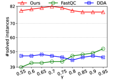
(a) 10th DIMACS (3-hour limit)

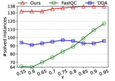
(b) real-world (3-hour limit)

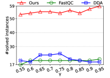
(c) 10th DIMACS (3-second limit)

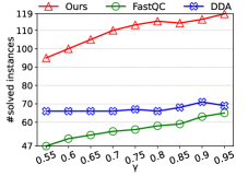
(d) real-world (3-second limit)

Figure 1. Number of solved instances with varying $\gamma$.

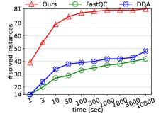
(a) $\gamma=0.65$

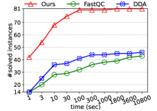
(b) $\gamma=0.75$

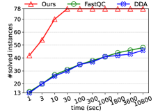
(c) $\gamma=0.85$

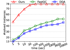
(d) $\gamma=0.95$

Figure 2. Number of solved instances on 10th DIMACS.

(a) $\gamma=0.65$

(b) $\gamma=0.75$

(c) $\gamma=0.85$

(d) $\gamma=0.95$

Figure 3. Number of solved instances on real-world.

Number of solved instances. We first compare our algorithm IterQC with the baselines DDA and FastQC by considering the number of instances solved within 3-hour and 3-second limit on two collections in Figure 1. In addition, we present the number of instances solved over time for both collections at $\gamma$ values of 0.65, 0.75, 0.85, and 0.95, in Figures 2 and 3. We have the following observations. First, our algorithm IterQC solves a greater number of instances across different values of $\gamma$, compared to the baselines FastQC and DDA. For example, in the real-world dataset with $\gamma=0.7$ (in Figure 1(b)), IterQC solves 135 out of 139 instances, while DDA and FastQC only solve 95 and 76 instances, respectively. Second, in general, as the value of $\gamma$ decreases, IterQC tends to use relatively larger values of $k$ during each iteration, leading to higher computational costs and longer overall running times. As shown in Figures 1(b), 1(c) and 1(d), the number of instances solved by IterQC generally increases with $\gamma$. However, this trend is less apparent in Figure 1(a). Specifically, as $\gamma$ decreases from 0.8 to 0.7, IterQC solves more instances. This phenomenon may be due to the following factors. IterQC computes a heuristic upper bound $ub$ in the preprocessing stage. The gap between this $ub$ and the optimum solution $s^{*}$ is unpredictable for different values of $\gamma$. A smaller gap may result in a potentially shorter overall running time. Additionally, in our graph reduction process in the preprocessing stage, a smaller $\gamma$ leads to a non-decreasing lower bound $lb$, which enhances the effectiveness of graph reduction and reduces subsequent search costs. Moreover, the increased computational complexity associated with smaller values of $\gamma$ primarily arises from the branch-and-bound search process. Intuitively, as $\gamma$ decreases, the relaxation of the clique condition becomes more significant, making it harder to prune branches that could previously be terminated early. The pseudo LB technique accelerates the branch-and-bound approach and helps reduce the increased difficulty introduced by smaller values of $\gamma$. Third, we observe in Figures 2 and 3 that the number of instances that IterQC can solve within 3 seconds exceeds the number solved by the other two baselines within three hours. For example, on the 10th DIMACS graphs with $\gamma=0.75$, IterQC solves 54 instances within 3 seconds, while DDA and FastQC solve 46 and 43 instances within 3 hours, respectively. Moreover, as shown in Figure 3(c), IterQC can complete 105 instances in 1 second, while DDA and FastQC finish 93 and 99 instances within 3 hours, respectively.

Performance on representative instances. The runtime performance comparison between IterQC and the two baseline algorithms with $\gamma=0.75$ across 30 representative instances is shown in Table 2. As illustrated in the table, IterQC consistently demonstrates superior efficiency, outperforming both baselines FastQC and DDA across nearly all instances. In particular, IterQC can solve all the graph instances, while both baseline algorithms FastQC and DDA exhibit a high occurrence of timeouts, failing to yield solutions within the 3-hour limit. Specifically, FastQC and DDA fail to solve 23 and 16 instances, respectively. Furthermore, IterQC successfully solves 14 out of the 30 representative instances where both baseline algorithms exceed the 3-hour time limit. For example, on G3, IterQC uses only 0.37 second, while both baselines cannot complete in 3 hours, achieving at least a 29,000$\times$ speed-up. These results further suggest the efficiency superiority of IterQC over both baseline algorithms. The superior performance of IterQC, particularly compared to FastQC, may be due to the hereditary property of the $k$-plex, which allows for more efficient pruning during the branch-and-bound search. However, in rare cases, the computational overhead of IterQC exceeds that of DDA, such as in G19, G23, and G26. This is because DDA adopts an iterative approach based on the IP solver CPLEX, which differs fundamentally from the branch-and-bound-based approaches used by IterQC and FastQC. As a general-purpose solver, CPLEX is not specifically optimized for the $\gamma$-quasi-clique problem and is difficult to tailor for it. Consequently, while DDA may occasionally perform better in specific instances, IterQC generally outperforms DDA in most cases.

Table 2. Runtime performance (in seconds) of IterQC, FastQC, and DDA on 30 instances with $\gamma=0.75$.

ID	IterQC	FastQC	DDA	ID	IterQC	FastQC	DDA
G1	0.03	OOT	0.16	G16	5.70	OOT	OOT
G2	0.004	652.72	0.10	G17	0.24	1073.59	0.34
G3	0.37	OOT	OOT	G18	341.59	OOT	OOT
G4	0.02	4.93	69.71	G19	4.06	OOT	2.73
G5	0.91	OOT	OOT	G20	1.38	OOT	1.49
G6	4.46	80.61	OOT	G21	1.87	OOT	2.14
G7	0.24	OOT	3059.20	G22	8.70	OOT	OOT
G8	0.32	OOT	OOT	G23	3.98	OOT	3.45
G9	0.02	3.88	0.20	G24	13.07	OOT	OOT
G10	2.46	OOT	OOT	G25	18.00	OOT	9.30
G11	17.71	OOT	OOT	G26	14.86	OOT	OOT
G12	0.41	OOT	OOT	G27	18.64	OOT	OOT
G13	0.26	34.60	297.66	G28	4.75	OOT	42.54
G14	3.28	106.46	OOT	G29	9.377	OOT	9.378
G15	772.93	OOT	OOT	G30	25.50	OOT	OOT

Scalability test. We use G30 for the scalability test, which has the most vertices among the representative graphs. In our experiment, we randomly extract 20% to 100% of the vertices and test the performance of IterQC and two baselines with $\gamma$ values of 0.65, 0.75, 0.85, and 0.95 in Figure 4. The results demonstrate two findings: First, in almost all cases, IterQC consistently achieves the shortest runtime. Second, across all four different values of $\gamma$, as the ratio increases—indicating a larger graph size – the increase in the runtime of IterQC is significantly smaller compared to the other algorithms. For example, in Figure 4(c), when the ratio increases from 0.2 to 0.8, the runtime of DDA rises from 0.52 seconds to 1817.60 seconds, whereas IterQC only increases from 0.49 seconds to 8.36 seconds. As for FastQC, at a ratio of 0.2, the runtime is 1086.88 seconds, but when the ratio reaches 0.4, it exceeds the time limit (10,800 seconds). These results demonstrate the scalability of IterQC.

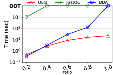
(a) $\gamma=0.65$

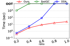
(b) $\gamma=0.75$

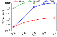
(c) $\gamma=0.85$

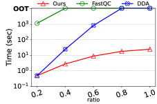
(d) $\gamma=0.95$

Figure 4. Scalability test on G30.

5.2. Ablation Studies

We conduct ablation studies to evaluate the effectiveness of the techniques of preprocessing and pseudo LB proposed in Section 4. We compare IterQC with the following variants:

• IterQC-PP: it removes the preprocessing technique in IterQC, which includes (1) the initial estimation of lower and upper bounds, and (2) graph reduction. Specifically, IterQC-PP replaces Lines 1-3 in Algorithm 2 with $ub\leftarrow|V|$.

• IterQC-PLB: it removes the pseudo lower bound $pseudo\mbox{-}lb$ and utilizes the true heuristic lower bound by replacing Line 3 in Algorithm 3 with $pseudo\mbox{-}lb\leftarrow lb\mbox{-}plex$.

Table 3 presents the runtime performance of IterQC, IterQC-PP, and IterQC-PLB on 30 representative instances with $\gamma=0.75$.

Table 3. Runtime performance (in seconds) of IterQC, IterQC-PP, and IterQC-PLB on 30 instances with $\gamma=0.75$.

ID	IterQC	-PP	-PLB	ID	IterQC	-PP	-PLB
G1	0.034	0.10	0.035	G16	5.70	35.54	6.31
G2	0.0043	0.039	0.0044	G17	0.24	2.96	0.32
G3	0.37	2.21	0.41	G18	341.59	4946.34	OOT
G4	0.019	0.08	0.015	G19	4.06	16.96	4.14
G5	0.91	6.64	0.80	G20	1.38	17.11	1.73
G6	4.46	6.65	4.86	G21	1.87	29.47	2.50
G7	0.24	1.36	0.17	G22	8.70	49.07	9.29
G8	0.32	1.24	0.61	G23	3.98	37.37	5.15
G9	0.021	0.17	0.018	G24	13.07	53.49	14.76
G10	2.46	2.51	29.79	G25	18.00	81.90	18.60
G11	17.71	97.73	134.01	G26	14.86	113.84	16.36
G12	0.41	1.05	0.66	G27	18.64	79.77	21.07
G13	0.26	0.99	0.22	G28	4.75	87.08	4.94
G14	3.28	11.15	3.42	G29	9.38	191.62	9.99
G15	772.93	1385.18	OOT	G30	25.50	195.29	25.97

Effectiveness of the preprocessing technique. From Table 3, we observe that IterQC consistently outperforms IterQC-PP, achieving a speedup factor of at least 5 in 17 instances and at least 10 in 6 instances, with a remarkable speedup factor of 20.32 on G29. We also summarize additional information for our preprocessing technique in Table 4, which details the percentages of vertices and edges pruned during preprocessing, as well as the lower and upper bounds ($lb$ and $ub$) for the optimum solution $s^{*}$. From Table 4, we observe that in 3 instances (G17, G20, and G29), the preprocessing technique prunes all vertices and edges, effectively obtaining the solution directly, while in 15 instances, it removes at least 90% of the vertices. Moreover, across the 30 instances, the preprocessing technique enables the iteration process to start from a smaller initial value (closer to the optimum solution $s^{*}$), as indicated by the upper bound $ub$ (in contrast to the trivial upper bound $|V|$ in Table 1).

Table 4. Preprocessing information with $\gamma=0.75$, where Red-V/Red-E represent the percentages of reduced vertices/edges.

ID	Red-V (%)	Red-E (%)	$lb$	$ub$	$s^{*}$
G1	98.29	87.61	116	119	117
G2	80.85	62.72	230	233	230
G3	65.86	46.16	74	87	74
G4	98.38	84.10	17	31	21
G5	60.22	39.17	57	84	66
G6	1.56	0.84	24	48	30
G7	93.32	77.40	54	71	59
G8	96.85	67.91	57	91	58
G9	98.36	97.56	6	7	6
G10	96.15	63.47	29	79	33
G11	42.27	8.76	13	124	45
G12	98.08	86.33	37	69	45
G13	0.00	0.00	3	7	6
G14	0.00	0.00	6	13	10
G15	97.49	53.99	86	316	127
G16	99.79	95.67	2209	2945	2209
G17	100.00	100.00	5	5	5
G18	76.82	52.51	66	308	130
G19	99.87	99.84	20	27	25
G20	100.00	100.00	5	5	5
G21	25.34	23.82	3	5	5
G22	0.00	0.00	2	4	2
G23	0.00	0.00	2	5	5
G24	0.00	0.00	2	4	2
G25	99.99	99.99	25	28	27
G26	1.15	1.15	5	7	6
G27	0.00	0.00	2	4	2
G28	29.35	24.36	3	5	5
G29	100.00	100.00	5	5	5
G30	99.72	98.72	10	23	10

Effectiveness of the pseudo LB technique. We can see in Table 3 that applying the pseudo LB technique leads to an improved performance in 25 of these 30 instances. Moreover, compared to IterQC-PLB, IterQC successfully solves 2 additional OOT instances, i.e., G15 and G18. For G18, IterQC solves in 341.59 seconds while IterQC-PLB times out, implying a speedup factor of at least 31.62. This improvement is due to the acceleration of the branch-and-bound search by the pseudo LB technique in Algorithm 3, particularly by leveraging the graph structure: dense local regions increase branch-and-bound search costs, leading to greater speedups. Conversely, instances like G4, G5, G7, G9, and G13 show lower effectiveness when the running time is dominated by the computations of the heuristic lower bound in Line 4 of Algorithm 3. Despite this, even in these instances, the impact on running time is minor, with all such instances completing in under 1 second.

6. Related Work

Maximum $\gamma$-quasi-clique search problem. The maximum $\gamma$-quasi-clique search problem is NP-hard (Matsuda et al., 1999; Pastukhov et al., 2018) and W[1]-hard parameterized by several graph parameters (Baril et al., 2021, 2024). The state-of-the-art exact algorithm for solving this problem is DDA (Pastukhov et al., 2018) and extensively discussed in Section 1. In contrast, Bhattacharyya and Bandyopadhyay (Bhattacharyya and Bandyopadhyay, 2009) provided a greedy heuristic. Further studies (Chou et al., 2015; Lee and Lakshmanan, 2016) addressed related problems of finding the largest maximal quasi-cliques that include a given target vertex or vertex set in a graph. Moreover, Marinelli et al. (Marinelli et al., 2021) proposed an IP-based method to compute upper bounds for the maximum $\gamma$-quasi-clique.

Maximal $\gamma$-quasi-clique enumeration problem. A closely related problem is the enumeration of all maximal $\gamma$-quasi-cliques in a given graph (Liu and Wong, 2008; Khalil et al., 2022; Yu and Long, 2023a), where a $\gamma$-QC $g$ is maximal if no supergraph $g^{\prime}$ of $g$ is also a $\gamma$-QC. Several branch-and-bound algorithms have been proposed to tackle this problem by using multiple pruning techniques to reduce the search space during enumeration. In particular, Liu and Wong (Liu and Wong, 2008), Guo et al. (Guo et al., 2020), and Khalil et al. (Khalil et al., 2022) developed such algorithms to improve efficiency. Recently, Yu and Long (Yu and Long, 2023a) introduced FastQC, the current state-of-the-art algorithm combining pruning and branching co-design approach. We remark that the maximum $\gamma$-QC search problem can be solved using algorithms designed for maximal $\gamma$-QC enumeration, as the maximum $\gamma$-QC is always a maximal one in the graph. In our experimental studies, we adapt the state-of-the-art maximal $\gamma$-QC enumeration algorithm, FastQC, as the baseline method to solve our problem. Some studies explored different problem variants. For example, Sanei-Mehri et al. (Sanei-Mehri et al., 2021) focused on the top-$k$ variant, Guo et al. (Guo et al., 2022) studied the problem in directed graphs, and others considered graph databases instead of a single graph (Jiang and Pei, 2009; Zeng et al., 2007).

Other cohesive subgraph mining problems. Another approach to cohesive subgraph mining involves relaxing the clique definition from the perspective of edges. This approach gives rise to the concept of the edge-based $\gamma$-quasi-clique (Abello et al., 2002; Conde-Cespedes et al., 2018; Pattillo et al., 2013), which is also referred to as pseudo-cliques (Uno, 2010), dense subgraphs (Long and Hartman, 2010), or near-cliques (Brakerski and Patt-Shamir, 2011; Tadaka and Kinoshita, 2016). In this cohesive subgraph model, the total number of edges in a subgraph must be at least $\gamma\cdot\binom{n}{2}$. Very recently, Rahman et al. (Rahman et al., 2024) introduced a novel pruning strategy based on Turán’s theorem (Jain and Seshadhri, 2017) to obtain an exact solution, building on the PCE algorithm proposed by Uno (Uno, 2010). Similar to the $\gamma$-quasi-clique problem, several studies have also explored non-exact approaches to solve the edge-based $\gamma$-quasi-clique problem (Abello et al., 2002; Brunato et al., 2008; Chen et al., 2021a; Liu et al., 2024). For instance, Tsourakakis et al. (Tsourakakis et al., 2013) proposed an objective function that unifies the concepts of average-degree-based quasi-cliques and edge-based $\gamma$-quasi-clique. There also exist many other types of cohesive subgraphs, including $k$-plex (Dai et al., 2022b; Wang et al., 2022; Zhou et al., 2020; Chang et al., 2022; Gao et al., 2018; Jiang et al., 2023, 2021; Wang et al., 2023; Xiao et al., 2017; Zhou et al., 2021), $k$-defective clique (Chang, 2023; Dai et al., 2023a; Gao et al., 2022), and densest subgraph (Ma et al., 2021; Xu et al., 2024). Moreover, the topic of cohesive subgraphs has also been widely studied in other types of graphs, including bipartite graphs (Chen et al., 2021b; Dai et al., 2023b; Luo et al., 2022; Yu et al., 2022; Yu and Long, 2023b; Yu et al., 2023), directed graphs (Gao et al., 2024), temporal graphs (Bentert et al., 2019), and uncertain graphs (Dai et al., 2022a). For an overview on cohesive subgraphs, see the excellent books and survey, e.g., (Chang and Qin, 2018; Fang et al., 2020, 2021; Huang et al., 2019; Lee et al., 2010).

7. Conclusion

In this paper, we studied the maximum $\gamma$-quasi clique problem and proposed an iterative framework incorporating two novel techniques: the pseudo lower bound and preprocessing. Extensive experiments demonstrated the superiority of our algorithm IterQC over state-of-the-art methods DDA and FastQC. In future work, we aim to extend our iterative approach to other cohesive graph models.

Appendix A Omitted Proofs

A.1. Omitted Proofs in Section 3

Proof of Lemma 3.2.

When $G$ is a $\gamma$-quasi-clique, we have $d_{G}(v)\geq\gamma\cdot(|V|-1)$, $\forall v\in V$. Since $d_{G}(v)$ is an integer for each $v\in V$, it follows that $d_{G}(v)\geq\lceil\gamma\cdot(|V|-1)\rceil\geq|V|-(\lfloor(1-\gamma)\cdot(|V|-1)\rfloor+1)=|V|-k_{1}$. Thus, $G$ is a $k_{1}$-plex and $\texttt{solve-k}(k_{1})=|V|$, which implies that $s_{1}=s_{0}$. At this point, we have $k_{1}=\texttt{get-k}(s_{1})$, and the algorithm results in $s_{1}=|V|$, which completes the proof. ∎

Proof of Lemma 3.3.

Assume, to the contrary, that $s_{i}=s_{i+1}$ for $0\leq i\leq p-1$. Then, it follows that $k_{i+1}=\texttt{get-k}(s_{i})=\texttt{get-k}(s_{i+1})$, which satisfies the termination condition in Line 4. This implies that the algorithm terminates at the $(i+1)$-st iteration, thus $i=p$, leading to a contradiction to $i\leq p-1$. ∎

Proof of Corollary 3.5.

By Lemma 3.4, the sequence is strictly decreasing. Further, it is easy to see that $s_{p}\geq 1$ since an induced subgraph with a single vertex is a trivial solution to the maximum $k$-plex problem with any $k\geq 1$. Moreover, as $\{s_{0},s_{1},\ldots,s_{p}\}$ is an integer sequence, the difference between any two consecutive elements is at least 1, which implies that $p\leq s_{0}=|V|=n$. ∎

Proof of Lemma 3.6.

Recall that $s^{*}$ is the size of the optimum solution. Let $u$ be the vertex with the minimum degree in the largest $\gamma$-quasi-clique $g^{*}$. Let $\gamma^{*}=\frac{d_{g^{*}}(u)}{s^{*}-1}$. Then we have $s^{*}=\texttt{solve-plex}\left(1+\left\lfloor(1-\gamma^{*})\cdot(s^{*}-1)\right\rfloor\right)$. Additionally, from the definition of a $\gamma$-quasi-clique, it also follows that $\gamma^{*}\geq\gamma$. We then use the mathematical induction to prove.
\scriptsize{1}⃝  $i=0$. $s_{i}=s_{0}=|V|\geq s^{*}$. The base case holds true.
\scriptsize{2}⃝  $i\geq 1$. Assume that the induction holds for $i-1$, i.e., $s_{i-1}\geq s^{*}$, it follows that

$$s_{i} =\texttt{solve-plex}(k_{i})=\texttt{solve-plex}(\texttt{get-k}(s_{i-1}))$$

$$=\texttt{solve-plex}\left(1+\left\lfloor(1-\gamma)\cdot(s_{i-1}-1)\right\rfloor\right)$$

$$\geq\texttt{solve-plex}\left(1+\left\lfloor(1-\gamma^{*})\cdot(s_{i-1}-1)\right\rfloor\right)$$

$$\geq\texttt{solve-plex}\left(1+\left\lfloor(1-\gamma^{*})\cdot(s^{*}-1)\right\rfloor\right)=s^{*}.$$

Based on \scriptsize{1}⃝, \scriptsize{2}⃝, and the principle of mathematical induction, we complete the proof of Lemma 3.6. ∎

A.2. Correctness Proof of Algorithm 4

We first show a property on the sequence generated by our basic iterative framework in Algorithm 1. To simplify the proofs, in the following discussion, let $s_{p}$ denote the last element of the sequence $\{s_{0},s_{1},\ldots,s_{p}\}$ generated by the iterative frameworks (either Algorithm 1 or Algorithm 4). It is important to highlight that, in contrast to $s_{p}$ in the correctness proof of the basic iterative framework, which represents the penultimate computed value, here $s_{p}$ specifically corresponds to the value at the iteration where Algorithm 3 terminates, i.e., $k_{p}=\texttt{get-k}(s_{p})$.

Lemma 0.

For any integer $\overline{s}\geq s^{*}$, the last element $s_{p}$ of the sequence $\{\overline{s},s_{1},s_{2},\ldots,s_{p}\}$ generated by Algorithm 1 is equal to $s^{*}$.

Proof.

The proof is similar to the proofs of Lemmas 3.6 and 3.7, which are based on a trivial upper bound, i.e., $|V|\geq s^{*}$. By using $\overline{s}$ instead of $|V|$, we can prove Lemma A.1. ∎

Subsequently, in Lemma A.2, we make a connection between the sequences generated by Algorithm 1 and Algorithm 4.

Lemma 0.

Consider the $i$-th iteration of Lines 2-6 in Algorithm 4, where Plex-Search$(G,k,ub\mbox{-}plex)$ is called in Line 3. We let $\overline{s}\leftarrow\texttt{solve-plex}(k)$, i.e., $\overline{s}$ is the size of maximum $k$-plex. If we have $k=\texttt{get-k}(ub\mbox{-}plex)$ and $ub\mbox{-}plex=s_{i-1}\geq s^{*}$, then $s_{i}\geq\overline{s}\geq s^{*}$.

Proof.

In Algorithm 3, we invoke the branch-and-bound algorithm Plex-BRB with a pseudo lower bound of $pseudo\mbox{-}lb$ in Line 4, where $pseudo\mbox{-}lb=\lfloor(lb\mbox{-}plex+ub\mbox{-}plex)/2\rfloor$ is not the true lower bound. In other words, with $pseudo\mbox{-}lb$, the size of the returned vertex set $S$ may not be larger than our pseudo lower bound $pseudo\mbox{-}lb$. We have two possible cases as follows.

1. $\overline{s}>pseudo\mbox{-}lb$. In this case, since the pruning in Plex-BRB using $pseudo\mbox{-}lb$ does not affect the generation of the correct solution of maximum $k$-plex, the returned vertex set $S$ from Plex-BRB corresponds to the maximum $k$-plex. Thus, we have $|S|=\overline{s}$. Moreover, as $s_{i}=\max\{pseudo\mbox{-}lb,|S|\}$, we know that $s_{i}\geq\overline{s}$.

2. $\overline{s}\leq pseudo\mbox{-}lb$. In this case, in Line 4 of Algorithm 4, we have $s_{i}=\max\{pseudo\mbox{-}lb,|S|\}$, which directly implies that $s_{i}\geq\overline{s}$.

In either case mentioned above, we have $s_{i}\geq\overline{s}$. According to Lemmas 3.6 and A.1 and $ub\mbox{-}plex=s_{i-1}\geq s^{*}$, we know that $\overline{s}\geq s^{*}$. The proof is thus complete. ∎

Utilizing the connection, we verify the correctness of Algorithm 4 that uses the technique of pseudo LB in the following.

Lemma 0.

Algorithm 4 correctly finds the largest $\gamma$-quasi-clique.

Proof.

According to Lemma A.2, we can guarantee that $s_{i}\geq s^{*}$ for each iteration $i$ in Lines 2-6 of Algorithm 4. Thus, we can view Algorithm 4 as a procedure that continuously seeks upper bounds for the maximum $\gamma$-quasi-clique across all iterations. Let $s_{p}$ denote the last element of the sequence $\{s_{0},s_{1},\ldots,s_{p}\}$ generated by Algorithm 4. Next, we prove that $s_{p}$ is equal to $s^{*}$.

Consider the $i$-th iteration in Lines 2-6 of Algorithm 4, where Plex-Search$(G,k,ub\mbox{-}plex)$ is called in Line 3. Note that $ub\mbox{-}plex=s_{i-1}$. We focus on this Plex-Search and have two cases.

1. $lb\mbox{-}plex=ub\mbox{-}plex$. Since $ub\mbox{-}plex=s_{i-1}$, it follows that $ub\mbox{-}plex=s_{i-1}\geq s^{*}$. We also know that there exists a $k$-plex of size $lb\mbox{-}plex$ computed in Line 1 of Algorithm 3. Thus, we have a $k$-plex of size $s_{i-1}$, where $k=\texttt{get-k}(s_{i-1})$. Similar to Lemma 3.7, it is easy to conclude that the returned result in Line 5 of Algorithm 4 is exactly $s^{*}$. Thus, $s^{*}=s_{i-1}=s_{i}$.

2. $lb\mbox{-}plex<ub\mbox{-}plex$. It is easy to see that $pseudo\mbox{-}lb<ub\mbox{-}plex$. If $s_{i}=pseudo\mbox{-}lb$ in Line 3 of Algorithm 4, it guarantees that $s_{i}<s_{i-1}$. Otherwise, i.e., $s_{i}=pseudo\mbox{-}size$, we use $\overline{s}_{i}$ to denote the size of the largest $k$-plex in the graph $G$, according to the proof of Lemma A.2, $s_{i}=\overline{s_{i}}$, which still satisfies $s_{i}=\overline{s_{i}}<s_{i-1}$. Thus, in any case, we have $s_{i}<s_{i-1}$.

Since $\{s_{0},s_{1},\ldots,s_{p}\}$ is an integer sequence with each $s_{i}\geq s^{*}$, the case in 2) is always finite. In other words, the case in 1) will definitely occur. The proof is complete. ∎

Appendix B Omitted Examples

Example of the basic iterative framework.

(a) An example graph.

(b) Illustration of the example.

Figure 5. An example of Algorithm 1 with $\gamma=0.55$.

We present an example of Algorithm 1 and illustrate its iterative process in Figures 5(a) and 5(b), respectively. In this example with $\gamma=0.55$, the graph has 8 vertices, which means $s_{0}=8$. By applying $k_{1}=\texttt{get-k}(s_{0})=\lfloor(1-0.55)\cdot(8-1)\rfloor+1=4$, the function solve-plex identifies the largest 4-plex, highlighted by the light-colored box in Figure 5(a), which results in $s_{1}=7$. Subsequently, $k_{2}=\texttt{get-k}(s_{1})=\lfloor(1-0.55)\cdot(7-1)\rfloor+1=3$, and solving solve-plex produces the largest 3-plex, indicated by the dark-colored box in Figure 5(a), with $s_{2}=6$ vertices. At this point, the stopping condition $k_{2}=\texttt{get-k}(s_{2})$ is satisfied, and the iteration terminates. The maximum 3-plex shown in Figure 5(a) corresponds to the desired maximum $0.55$-quasi-clique. In Figure 5(b), the horizontal axis represents $k$, while the vertical axis represents $n$. Moreover, (1) the sparse light blue dashed line shows the relationship between $n$ and the corresponding $k$ obtained from get-k; (2) the dense red dashed line shows the relationship between $k$ and the resulting $n$ obtained from solve-plex; (3) the green solid line represents the overall iterative process of Algorithm 1, demonstrating how $n$ evolves from the initial graph of size 8 to the final result of the maximum $\gamma$-quasi-clique with size 6. Specifically, we start with $s_{0}=8$. After the first iteration, applying get-k($s_{0}$) transitions to the state to $(4,8)$ in Figure 5(b) on the corresponding axes (i.e., $k_{1}=4$, $s_{0}=8$). Then, solving $s_{1}=\texttt{solve-plex}(k_{1})$ transitions the state to $(4,7)$, completing one full iteration. Repeating this process leads to termination at $(3,6)$, where the corresponding vertical coordinate $6$ represents the optimum solution $s^{*}=6$.

Example of the pseudo LB technique.

(a) An example graph.

(b) Illustration of the example.

Figure 6. An example of Algorithm 4 with $\gamma=0.75$.

Figure 6(a) shows a graph with 7 vertices and Figure 6(b) presents the corresponding iterative process. For clarity, line segments near $k=2$ in Figure 6(b) are slightly shifted along the positive $k$-axis; this is solely for visualization and does not indicate non-integer $k$ values. Assume that the heuristic solution obtained in each iteration corresponds to the subgraph in the dark-colored box, i.e., $G[\{0,5,6\}]$, in Figure 6(a), where $lb\mbox{-}plex=3$ according to Line 1 of Algorithm 3. As shown in Figure 6(b), using the pseudo LB technique to solve the problem with $\gamma=0.75$ in Figure 6(a) requires two iterations. The first iteration, represented by the double-arrowed purple solid line in the figure, corresponds to the second case discussed in the proof of Lemma A.2. At this stage, $pseudo\mbox{-}lb=\lfloor(3+7)/2\rfloor=5>\overline{s}_{1}=4$. Consequently, the branch-and-bound search in Line 4 of Algorithm 3 fails to find a solution, resulting in $S=\emptyset$. Thus, $s_{1}=\max\{5,0\}=5$, which initiates the second iteration. In the second iteration, $pseudo\mbox{-}lb=\lfloor(5+3)/2\rfloor=4\leq\overline{s}_{2}=4$, which corresponds to the first case discussed in the proof of Lemma A.2. Since the pruning during the branch-and-bound search uses $pseudo\mbox{-}lb=3$, it does not affect the computation of the solution $S$. Thus, $s_{2}=\max\{3,4\}=4$, satisfying the condition in Line 4 of Algorithm 3. The final solution, i.e., $G[\{1,2,3,4\}]$, is in Figure 6(a) within the light-colored box.

Appendix C Additional Experiments

Number of solved instances. Figures 7 and 8 illustrate the trends in the number of solved instances over time for IterQC, FastQC, and DDA on the 10th DIMACS and real-world datasets, under $\gamma$ values of 0.55, 0.6, 0.7, 0.8, and 0.9. From these results, it is easy to see that under the same time constraint, for any given value of $\gamma$ or dataset, IterQC consistently solves more instances compared to the baseline algorithms. Remarkably, regardless of the dataset or $\gamma$, IterQC solves more instances within 3 seconds than the larger number achieved by either baseline algorithm within 3 hours. For instance, at $\gamma=0.6$, IterQC solves 53 instances in only 3 seconds, while FastQC and DDA solve only 41 and 58 instances, respectively, even after 3 hours of computation. Across all tested values of $\gamma$, IterQC achieves improved practical performance. On the 10th DIMACS dataset, it solves at least 79 out of 84 instances, while on the real-world dataset, it solves at least 132 out of 139 instances.

(a) $\gamma=0.55$

(b) $\gamma=0.6$

(c) $\gamma=0.7$

(d) $\gamma=0.8$

(e) $\gamma=0.9$

Figure 7. Number of solved instances on 10th DIMACS graphs.

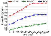
(a) $\gamma=0.55$

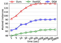
(b) $\gamma=0.6$

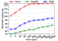
(c) $\gamma=0.7$

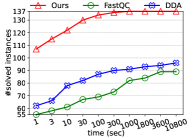
(d) $\gamma=0.8$

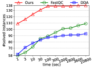
(e) $\gamma=0.9$

Figure 8. Number of solved instances on real-world graphs.

Performance on representative instances. Tables 5 and 6 summarize the performance of IterQC and the two baseline algorithms across 30 representative instances under $\gamma$ values of 0.65 and 0.85. The results demonstrate that IterQC consistently outperforms the baseline algorithms in terms of solving capability within the given time limit of 3 hours. In particular, IterQC successfully solves all instances except for G29 under $\gamma=0.65$, achieving nearly complete coverage. In contrast, the two baseline algorithms, FastQC and DDA, exhibit a significant number of timeouts under all values of $\gamma$. For instance, at $\gamma=0.65$, FastQC and DDA fail to solve 25 and 18 instances, respectively, out of the 30 cases. These results highlight the robustness and efficiency of IterQC in handling challenging instances, further validating its scalability and superiority over the baseline methods. On the other hand, we can observe that in most cases, as $\gamma$ increases, the runtime of FastQC gradually decreases, as seen in instances like G4 and G5, or the difference remains small, as in G13, G14, and G17. However, for the IterQC algorithm, the trend may not always be monotonic, as shown in instances like G15 and G16. This is because IterQC starts iterating from an upper bound, and its performance is influenced by both the core number and $\gamma$ in a heuristic manner. If the initial bound is already close to the final solution, the algorithm can converge in just a few iterations. As a result, $\gamma$ not only affects the complexity of the search space but also impacts the number of iterations in IterQC, making its runtime not necessarily monotonic with respect to $\gamma$.

Table 5. Runtime performance (in seconds) of IterQC, FastQC, and DDA on 30 instances with $\gamma=0.65$.

ID	IterQC	FastQC	DDA	ID	IterQC	FastQC	DDA
G1	0.008	OOT	0.25	G16	6.49	OOT	OOT
G2	6.19	OOT	1.04	G17	0.04	1041.55	3.22
G3	0.55	OOT	OOT	G18	OOT	OOT	OOT
G4	0.03	2211.78	101.39	G19	13.80	OOT	26.85
G5	6.07	OOT	OOT	G20	2.42	OOT	13.39
G6	OOT	OOT	OOT	G21	6.47	OOT	21.64
G7	0.33	OOT	OOT	G22	9.70	OOT	6845.3
G8	5.33	OOT	OOT	G23	0.30	OOT	26.90
G9	0.01	3.89	1.92	G24	4.82	OOT	OOT
G10	4.08	OOT	OOT	G25	1.80	OOT	91.48
G11	135.1	OOT	OOT	G26	0.49	OOT	OOT
G12	3.38	OOT	OOT	G27	26.13	OOT	OOT
G13	5.87	33.99	OOT	G28	19.65	OOT	40.70
G14	5.01	98.83	OOT	G29	36.31	OOT	OOT
G15	3.06	OOT	OOT	G30	23.28	OOT	OOT

Table 6. Runtime performance (in seconds) of IterQC, FastQC, and DDA on 30 instances with $\gamma=0.85$.

ID	IterQC	FastQC	DDA	ID	IterQC	FastQC	DDA
G1	0.08	OOT	3.43	G16	6.49	OOT	OOT
G2	5.02	OOT	0.88	G17	0.015	1115.24	517.41
G3	0.30	OOT	OOT	G18	91.45	OOT	OOT
G4	0.02	1.18	21.53	G19	12.32	OOT	16.63
G5	0.50	85.27	OOT	G20	2.65	OOT	OOT
G6	5.01	5.05	OOT	G21	13.03	OOT	21.88
G7	0.21	203.62	OOT	G22	18.28	OOT	OOT
G8	5.13	OOT	OOT	G23	0.24	OOT	25.93
G9	0.13	3.90	0.48	G24	8.84	OOT	OOT
G10	4.14	OOT	OOT	G25	1.90	OOT	46.32
G11	7.95	OOT	OOT	G26	0.38	OOT	OOT
G12	0.45	OOT	OOT	G27	29.11	OOT	OOT
G13	5.90	34.95	2490.8	G28	17.61	OOT	39.78
G14	3.48	102.83	OOT	G29	0.99	OOT	93.58
G15	0.19	OOT	OOT	G30	21.31	OOT	OOT

Ablation studies. Tables 7 to 8 present the results of the ablation studies conducted on 30 representative instances, demonstrating the impact of preprocessing and the pseudo lower bound (pseudo LB) techniques on practical performance. The results clearly indicate significant improvements across all values of $\gamma$. For the preprocessing technique, the optimization effect is clear in nearly every case. For example, at $\gamma=0.65$, instance G29 achieves a speedup of approximately $20.79\times$ compared to the setting without the preprocessing technique. Regarding the pseudo LB technique, substantial benefits are observed in most instances, particularly for smaller values of $\gamma$. At $\gamma=0.65$, 23 out of 30 instances show accelerated running time. Specifically, for G11 at $\gamma=0.65$ and G15 at $\gamma=0.85$, the introduction of the pseudo LB technique transforms previously unsolvable instances within the 3-hour limit into solvable ones. For G15 at $\gamma=0.85$, the running time is reduced to 57.88 seconds, corresponding to a speedup of $186\times$. These findings highlight the critical contributions of both preprocessing and pseudo LB techniques in improving efficiency of the proposed method.

Table 7. Runtime performance (in seconds) of IterQC, IterQC-PP, and IterQC-PLB on 30 instances with $\gamma=0.65$.

ID	IterQC	-PP	-PLB	ID	IterQC	-PP	-PLB
G1	0.01	0.1	0.01	G16	5.87	102.0	6.52
G2	0.01	0.07	0.01	G17	0.3	4.95	0.28
G3	0.55	2.11	0.55	G18	OOT	OOT	OOT
G4	0.04	0.18	0.05	G19	4.08	29.05	4.33
G5	6.07	10.14	14.32	G20	1.8	32.42	2.71
G6	6.19	7.53	6.47	G21	2.42	73.74	2.95
G7	0.33	1.57	0.23	G22	4.82	77.83	6.55
G8	3.06	4.07	12.26	G23	5.33	90.88	5.93
G9	0.02	0.23	0.03	G24	6.47	79.45	7.78
G10	36.31	35.66	180.13	G25	19.65	144.75	19.2
G11	135.12	501.39	OOT	G26	26.13	159.5	29.94
G12	3.38	3.64	7.35	G27	9.7	116.42	11.26
G13	0.49	1.74	0.46	G28	6.49	134.9	6.57
G14	5.01	9.74	5.87	G29	13.8	368.1	13.91
G15	OOT	OOT	OOT	G30	23.28	460.12	27.91

Table 8. Runtime performance (in seconds) of IterQC, IterQC-PP, and IterQC-PLB on 30 instances with $\gamma=0.85$.

ID	IterQC	-PP	-PLB	ID	IterQC	-PP	-PLB
G1	0.08	0.14	0.1	G16	5.9	17.33	6.34
G2	0.13	0.46	0.13	G17	0.24	1.67	0.26
G3	0.3	0.86	0.28	G18	91.45	5334.55	74.72
G4	0.01	0.08	0.02	G19	4.14	12.31	5.96
G5	0.5	3.15	0.38	G20	1.9	11.16	2.05
G6	5.02	7.39	2.83	G21	2.65	25.22	3.31
G7	0.21	0.85	0.14	G22	8.84	33.29	12.81
G8	0.19	0.81	0.17	G23	5.13	35.33	6.9
G9	0.02	0.09	0.02	G24	13.03	45.33	13.29
G10	0.99	1.64	3.51	G25	17.61	59.02	18.97
G11	7.95	92.42	7.42	G26	29.11	82.92	31.36
G12	0.45	1.12	0.4	G27	18.28	69.84	19.63
G13	0.38	0.94	0.44	G28	6.49	58.82	6.95
G14	3.48	7.3	4.13	G29	12.32	86.57	13.46
G15	57.88	107.74	OOT	G30	21.31	163.58	25.44

Performance on artificial datasets. We test our algorithms on synthetic graphs: Scale-Free (SF) graphs and Small-World (SW) graphs (Rahman et al., 2024). SF graphs are generated by the Barabási–Albert model with parameter $w$, starting from a star graph of $w$ vertices and incrementally adding new vertices, each connected to $w$ existing vertices, until the graph contains $n$ vertices. SW graphs are generated by the Watts–Strogatz model with rewiring probability $p$. It begins with a cycle graph of $n$ vertices, where each vertex is connected to its $d$ nearest neighbors, forming a ring lattice. Then, for each edge $(u,v)$, the endpoint $v$ is randomly rewired to a non-adjacent vertex with probability $p$. In general, the graphs become denser as $w$ or $d$ increases. We fix $n=10^{6}$, set $p=0.2,\gamma=0.75$, and vary $w$ and $d$ in $\{10,15,20,25,30\}$. The time limit is set to 3 hours (10,800 seconds). We report the running times in the Table 9.

We observe that our IterQC algorithm consistently outperforms all baseline methods. The running time of all algorithms increases with larger $w$ or $d$, as higher values of these parameters lead to denser graphs. Moreover, the performance gains of IterQC become more pronounced as $w$ increases in SF graphs and $d$ decreases in SW graphs. This is because a larger $w$ in SF graphs results in denser local structures, where the preprocessing step can effectively reduce the graph size. In contrast, while increasing $d$ in SW graphs adds more edges, the uniform structural properties limit the pruning effectiveness, resulting in less speedup.

Table 9. Runtime performance (in seconds) of IterQC, FastQC, and DDA on artificial datasets with $\gamma=0.75$.

SF				SW
$w$	IterQC	FastQC	DDA	$d$	IterQC	FastQC	DDA
10	0.14	9.59	OOT	10	0.18	4.44	OOT
15	0.30	18.56	OOT	15	0.26	4.66	OOT
20	0.52	32.66	OOT	20	0.35	5.39	OOT
25	0.63	57.33	1.06	25	0.88	6.05	OOT
30	0.93	146.74	OOT	30	1.83	7.29	OOT

Memory consumption. We evaluate the memory usage of IterQC and two baseline algorithms across 30 representative graphs, as reported in Table 10. Memory usage is measured as the peak memory consumption during execution. For baseline methods that encountered timeouts, we record the maximum memory usage observed prior to termination. We observe that the memory usage is comparable among all algorithms. In addition, we can prove that IterQC has the space complexity of $O(m+n)$, which is the same as the baselines and is linear with respect to the size of the input graph. The experimental results are aligned with the theoretical analysis.

Table 10. Memory consumption (in GB) of IterQC, FastQC, and DDA on 30 instances with $\gamma=0.75$.

ID	IterQC	FastQC	DDA	ID	IterQC	FastQC	DDA
G1	0.0	0.0	0.01	G16	1.73	6.06	0.92
G2	0.0	0.0	0.02	G17	0.11	0.2	0.12
G3	0.03	0.09	0.13	G18	3.63	11.56	2.46
G4	0.01	0.01	0.01	G19	1.08	16.14	0.48
G5	0.05	0.15	0.09	G20	0.57	2.06	0.59
G6	0.1	0.07	0.12	G21	0.88	3.19	0.95
G7	0.03	0.1	0.04	G22	1.11	3.69	16.17
G8	0.02	0.06	0.09	G23	1.13	3.93	1.09
G9	0.01	0.01	0.02	G24	1.46	4.89	21.1
G10	0.02	0.05	0.06	G25	4.66	16.14	1.88
G11	0.09	0.25	0.16	G26	2.45	7.54	32.57
G12	0.04	0.13	0.13	G27	1.95	6.48	29.26
G13	0.04	0.06	0.6	G28	1.87	6.69	1.91
G14	0.17	0.21	0.8	G29	3.75	13.56	3.98
G15	0.22	0.74	0.45	G30	5.21	18.99	9.17