Comparing Parameterizations and Objective Functions for Maximizing the Volume of Zonotopic Invariant Sets
Abstract
In formal safety verification, many proposed algorithms use parametric set representations and convert the computation of the relevant sets into an optimization problem; consequently, the choice of parameterization and objective function have a significant impact on the efficiency and accuracy of the resulting computation. In particular, recent papers have explored the use of zonotope set representations for various types of invariant sets. In this paper we collect two zonotope parameterizations that are numerically well-behaved and demonstrate that the volume of the corresponding zonotopes is log-concave in the parameters. We then experimentally explore the use of these two parameterizations in an algorithm for computing the maximum volume zonotope invariant under affine dynamics within a specified box constraint over a finite horizon. The true volume of the zonotopes is used as an objective function, along with two alternative heuristics that are faster to compute. We conclude that the heuristics are much faster in practice, although the relative quality of their results declines as the dimension of the problem increases; however, our conclusions are only preliminary due to so-far limited availability of compute resources.
I Introduction
A common approach to safety analysis and/or synthesis involves the computation of reachable, invariant, viable or discriminating sets. Nonparametric representations of such sets, such as implicit surface functions sampled on a grid [1], are general but scale poorly with dimension; consequently, much work has focused on parametric representations including polytopes [2, 3, 4], support functions [2, 5], and ellipsoids [6, 7, 8] because of their computational efficiency on some of the common set operations. Zonotopes, a class of polytopes, have attracted particular attention recently because of the flexibility and efficiency of their encoding, as well as the fact that they are closed under affine transformation and Minkowski sum [5, 9]. Starting with [10] for reachable sets, they have been used in a wide variety of set computations, particularly for systems with linear or affine dynamics.
While many algorithms construct their sets by stepping in time, the advent of powerful linear, convex and general nonlinear optimization tools has lead to a category of algorithms which seek to construct the sets through optimization. For example, in [11], they presented approaches to approximate viability kernels based on the computation of the region of attraction and then converted the problem to an infinite-dimensional linear programming problem in the cone of nonnegative occupation measures. Another use of convex optimization is presented in [12] to approximate polytopic discriminating kernels and the corresponding linear state feedback control law in a linear discrete-time system. The authors of [13] consider the computation of discriminating sets and the corresponding control law for systems with additive and bounded disturbances by constructing linear matrix inequalities optimization problem. Choice of efficient parameterization is the focus of [14], which considers the computation of discriminating sets for linear discrete-time feedback systems where they assume the discriminating sets are of low-complexity, namely symmetric around the origin and described by the same number of affine inequalities as twice the dimension of the state variables.
In the context of optimization, the question of parameterization is critical to efficient solution, since optimization cost is typically superlinear in the number of decision variables and constraints. In particular, two zonotope parameterizations have been used recently in the literature exploring invariant sets. Template zonotopes are used in [15]: Zonotopes whose generators are fixed but the scaling of those generators can be adjusted. Parallelotopes (a subclass of zonotopes) are used in [16]: Zonotopes whose generator matrix is upper triangular with positive entries along the diagonal. Both parameterizations can easily ensure that the zonotope volume does not collapse to zero, which is much more difficult to achieve with a general dense generator matrix.
Our contributions in this paper are to:
- •
-
•
Compare experimentally the use of these two parameterizations in an algorithm for computing a maximum volume zonotope invariant under affine, input-free dynamics in a given box constraint over finite horizon from [17]. For one of the parameterizations the true volume is computationally expensive to evaluate, so we also compare two heuristic objective functions for that parameterization.
II PRELIMINARIES
We define the invariance problem that we seek to solve, and the zonotope set representation and parameterizations that we use to solve it.
II-A Invariant Sets
In this paper we consider discrete-time, time-invariant affine dynamics
| (1) |
where represents the state at time , is the evolution matrix, and is the constant drift.
Given a system (1), a box constraint set
and a time , we would like to find a finite horizon invariant set.
Definition 1
A set is invariant in for horizon if for all and for all , .
There are contexts in which one might seek invariant sets with maximal or minimal volume, but in the remainder of this paper we focus on the former.
Define the forward reach set of some specified set as
| (2) |
Note that the reach set is defined at a single time rather than over a time interval, and the set is an initial condition rather than a constraint. We will use the reach set of to constrain to be invariant.
Proposition 2
A set is invariant in over horizon if for all , .
II-B Zonotope Representation
We choose to use the compact zonotope to represent our invariant sets. A zonotope can be characterized by its center and generator matrix as the set
For a zonotope with center and generator matrix , we will sometimes write . If the generator matrix is such that and —in other words, that is short and fat and has full column rank—then the corresponding zonotope is full dimensional.
For a zonotope with generator matrix and , its -dimensional volume can be computed by the formula [18]
| (3) |
where the summation is over the set of indexes such that and is the submatrix of consisting only of columns . Note that if we vary the entries of a generator matrix , the volume formula (3) discretely changes form (fewer columns are chosen) when the rank drops. In order to avoid such a complication, we choose constraints on the parameterizations of our zonotopes to ensure their generator matrices are of full rank.
In our search for invariant sets, we will consider two parameterizations of zonotopes. The distinction between the two lies in the choice of generator matrix; in both cases we allow the center vector to be chosen arbitrarily.
Upper Triangular Positive Definite (UTPD): Following [16] we constrain the generator matrix to be upper triangular with strictly positive entries along the diagonal; consequently, the generator matrix must be square and full rank, and the zonotope is a full dimensional parallelotope. For a zonotope , the corresponding UTPD matrix will have free variables and positivity constraints.
Scaled Fixed Generators (SFG): Following [15] but restricting entries to be real valued as in [17] we constrain the generator matrix to take the form where is fixed and is the diagonal scaling matrix with vector along its diagonal. If we choose to have full rank, then the constraint ensures that the product is also full rank. The corresponding zonotope is a full dimensional (real) template zonotope in the sense that the directions of the generators are fixed but their scaling is not. This parameterization has free parameters (the entries of ) and positivity constraints.
The order of a zonotope is defined as ; consequently, the UTPD parameterization is always order 1 while the SFG parameterization has the same order as the predefined .
III Invariant Set Construction as a Convex Optimization
For dynamics (1) it is straightforward to show that the reach set of an initial zonotope is itself a zonotope characterized by
| (4) | ||||
Using Proposition 2 and (4) we arrive at a set of constraints on to achieve invariance.
Proposition 3
These constraints are linear in the entries of and convex in the entries of . In fact, it can be shown that the constraints are linear in any components of with known sign; for example, the diagonal entries of in the UTPD parameterization or the entries of the scaling vector in the SFG parameterization.
Using Proposition 3, we can construct an optimization to find the largest invariant zonotope within our parameterized set of zonotopes.
| (6) | ||||
| such that | ||||
| and | ||||
For the UTPD and SFG parameterizations of , the rank constraint translates into linear inequalities, so (6) will be a convex optimization if the objective function is convex. We explore the implications for each of the parameterizations in the next subsections.
III-A Objective Functions for the UTPD Parameterization
The UTPD parameterization uses a square, upper-triangular generator matrix, so the sum in (3) collapses to a single term
| (7) | ||||
where is the diagonal element of and the final equality holds because the rank constraint for UTPD specifies .
Proposition 4
For the UTPD parameterization, the zonotope volume is log-concave (actually log-linear) in the free variables (the entries of the upper triangular generator matrix).
Proof:
The (identity) function is log-concave on for each , and the product of log-concave functions is log-concave. ∎
For UTPD the cost of evaluating the convex constraints (5) is , dominated by the cost of evaluating the term. The cost of evaluating the objective function (7) is .
Although [16] proposes a linear objective function for maximizing the volume of their zonotopes (allowing them to keep the continuous portion of their optimization linear), we do not further explore their objective function here because the true volume formula (7) is log-concave and so cheap to evaluate.
III-B Objective Functions for the SFG Parameterization
The SFG parameterization multiplies a fixed rectangular generator matrix by a positive scaling factor , so the summation in (3) is still present but can be simplified.
| (8) | ||||
where
is the volume of the parallelotope with (square) generator matrix , and is hence a fixed weight in (8) once the generator matrix is chosen. Note that unlike the (multiple) summation over the multiple indexes , the (single) product in (8) is over the single index and multiplies together the elements of the scaling vector .
Proposition 5
For the SFG parameterization, the zonotope volume is log-concave in the free variables (the entries of the scaling vector ).
Proof:
Assume without loss of generality that zonotope is centered at the origin, so . In the SFG parameterization,
Therefore, the indicator function for can be written as
Because we require to have full rank, there always exists (many) such that , but if then the constraints cannot be satisfied.
Following [19, Example 3.44] it can be shown that is log-concave in its arguments; thus,
is log-concave as a function of . ∎
For SFG the cost of evaluating the convex constraints (5) is the same as for UTPD: . However, there are
terms in (8) each of which is to evaluate (assuming that the constant weights are precomputed); consequently, the cost of evaluating (8) grows very fast for higher order zonotopes.
In order to reduce the computational cost of the objective function for the SFG parameterization, we propose two alternative heuristics:
-
•
Sum of scalars: Following the positive results reported in [17], use
(9) This choice is linear in and to evaluate.
-
•
Log sum of scalars: Following the observation that the true volume (8) is the sum of weighted products of subsets of the entries of , use
(10) This choice is log-linear in and to evaluate.
IV Experimental Comparison of Parameterizations and Objective Functions
In this section we experimentally compare the two parameterizations and three objective functions discussed in the previous section. The experiments were run on a MacBook Pro laptop with a 2.5 GHz quad-core Intel Core i7 processor and 16 GB of 1600 MHz DDR3 RAM under macOS Catalina (version 10.15.3). We used the Julia programming language [20] with the JuMP package [21] to formulate our optimizations and the Ipopt solver [22] on the backend.
IV-A Procedure
In every case we seek to solve the optimization (6) and thereby compute a maximum volume zonotope which is invariant in over horizon . The four cases we examine are:
-
•
SFG+ss: SFG parameterization with the sum of scalars heuristic objective function (9).
-
•
SFG+slgs: SFG parameterization with the product of scalars heuristic objective function (10). Because this heuristic is log-linear, in practice we use the objective (the sum of logs of scalars).
-
•
SFG+lgv: SFG parameterization with the true zonotope volume objective function (8). Because this function is log-concave, we maximize the log of the volume.
-
•
UTPD+lgv: UTPD parameterization with the true zonotope volume objective function (7). Because this function is log-concave, we maximize the log of the volume.
| trials | |||
|---|---|---|---|
| 3 | 3 | 2500 | 1 |
| 3 | 6 | 2500 | 20 |
| 3 | 8 | 2500 | 56 |
| 6 | 10 | 2500 | 210 |
| 8 | 13 | 100 | 1287 |
| 10 | 14 | 100 | 1001 |
| 12 | 15 | 100 | 455 |
| 15 | 16 | 100 | 16 |
We ran our comparison experiment on eight different combinations of as listed in Table I in order to explore the impact of the number of dimensions and the number of generators on the performance of different objective functions. We remind the reader that is only meaningful in the SFG parameterization, where the fixed generator matrix ; in the UTPD parameterization the number of generators is always .
In each trial, we generated a random stable dynamics matrix in (1) using a Julia reimplementation of Matlab’s rss command (with discrete time step size ). For the SFG parameterization we filled the first columns of the fixed generator matrix with the identity matrix of size , and any remaining columns for were filled with random unit vectors (different vectors for each trial). The constraint set was chosen as and the horizon .
IV-B Results
| SFG | UTPD | |||
|---|---|---|---|---|
| (,) | ss | slgs | lgv | lgv |
| (3, 3) | 6.29 | 6.33 | 6.33 | 6.67 |
| (3, 6) | 6.60 | 5.47 | 6.78 | " |
| (3, 8) | 6.86 | 5.32 | 7.07 | " |
| (6, 10) | 17.51 | 15.28 | 21.71 | 22.80 |
| (8, 13) | 15.71 | 18.81 | 26.22 | 29.30 |
| (10, 14) | 25.88 | 29.28 | 41.36 | 55.73 |
| (12, 15) | 22.33 | 31.40 | 39.03 | 84.39 |
| (15, 16) | 17.82 | 23.17 | 24.59 | 106.18 |
| SFG | UTPD | |||
|---|---|---|---|---|
| (,) | ss | slgs | lgv | lgv |
| (3, 3) | 0.01 | 0.02 | 0.04 | 0.22 |
| (3, 6) | 0.02 | 0.02 | 0.06 | " |
| (3, 8) | 0.02 | 0.02 | 0.08 | " |
| (6, 10) | 0.04 | 0.04 | 0.36 | 1.05 |
| (8, 13) | 0.07 | 0.07 | 3.65 | 2.80 |
| (10, 14) | 0.09 | 0.09 | 5.93 | 5.83 |
| (12, 15) | 0.13 | 0.13 | 5.82 | 10.75 |
| (15, 16) | 0.22 | 0.20 | 1.19 | 37.42 |


IV-C Analysis
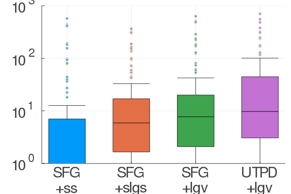
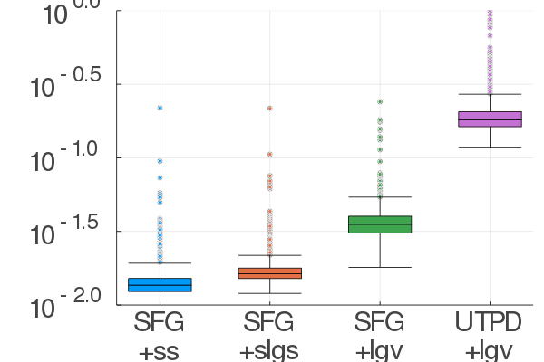
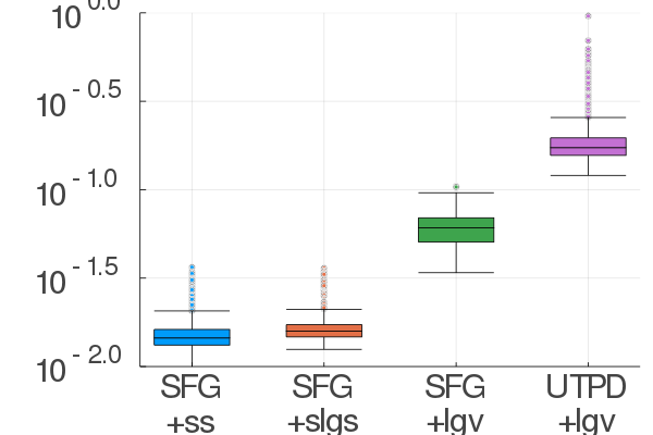
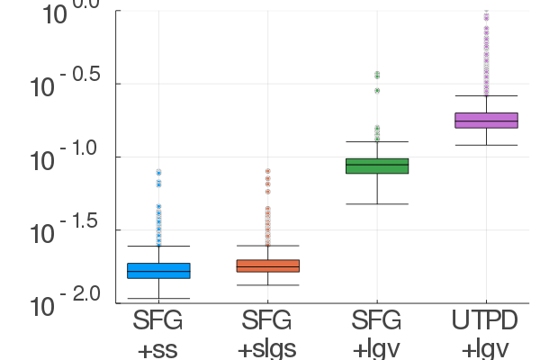
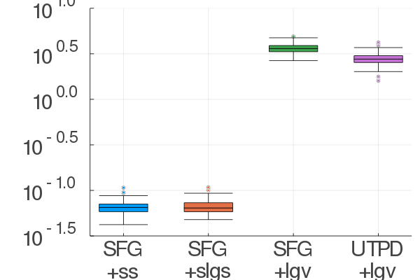
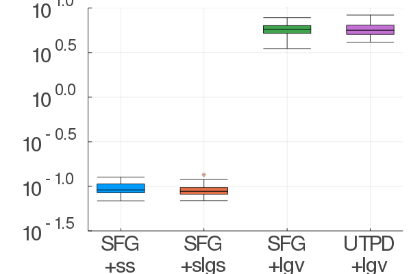
Looking first at the three cases where , we see in Table II that when then the UTPD+lgv combination produces a noticeably better volume, but as we increase the SFG+ss and SFG+lgv combinations match and then exceed the performance. Interestingly SFG+slgs actually performs worse on the higher order cases. We conjecture that this situation occurs because for higher orders there is more likely to be unproductive generators among those randomly chosen; allowing the scale factor for those generators to approach zero does not harm the ss or lgv objective functions but will significantly penalize the slgs objective function.
In contrast, as we increase we see a different trend. UTPD+lgv consistently outperforms the others, particularly as the order of the zonotopes for SFG drops towards 1. The SFG+slgs heuristic performs much closer to SFG+lgv than does the SFG+ss heuristic.
Examining the runtimes in Table III, we see the expected behaviour for the SFG parameterizations: The ss and slgs heuristic objective functions are similarly fast, and the lgv objective function cost shows dramatic effects of both increasing and (the latter explicitly computed for convenience in Table I). What is perhaps a little surprising is how the UTPD+lgv runtime is growing even faster than SFG+lgv as dimension increases, even though the objective function for the former is much cheaper to evaluate. We attribute this effect to the fact that the UTPD parameterization has decision variables, compared to for the SFG parameterization. Those extra decision variables produce much better zonotope volumes, but at a tremendous computational cost.
IV-D Limitations
The primary limitation of these experiments is that we considered a single algorithm to solve the single problem of finding a maximum volume zonotope invariant in a specified box constraint set over a fixed finite horizon for stable systems without inputs. Going forward, we plan to compare these parameterizations and objective functions for more general types of invariant sets and multiple algorithms.
For this preliminary set of experiments we had quite limited compute resources and hence were unable to properly explore the effects of changing and independently. We also chose the extra generators in the SFG parameterization randomly, but there are better options available; for example [15].
Finally, we considered only random dynamics in moderate dimensions. It would be good to explore whether these techniques are at all feasible for real problems with dozens to hundreds of dimensions, such as those mentioned in [23].
V Conclusions and Future Works
There has been considerable recent interest in using zonotopes for various forms of invariant and reachable sets in the past few years, and in several algorithms these zonotopes are constructed through optimizations. In this paper we described two different parameterizations of zonotopes that have been used for such algorithms, and observed that the volume of the zonotope in each case is a log-concave function of the parameters and hence is amenable to efficient maximization. For one particular invariant set algorithm, we explored four possible parameterization–objective function pairs: Both parameterizations with the true volume objective function, plus two heuristic objective functions for one of the parameterizations. Perhaps not surprisingly the heuristics were fastest, but the quality of their results began to suffer in higher dimensions, while the relative quality and runtime of the more flexible parameterization both increased with dimension.
In future work we plan to expand the range of experiments in terms of dimension and order of the zonotopes, choice of template directions for the generators, the types of invariant sets being computed and the algorithms being used.
References
- [1] I. M. Mitchell, A. M. Bayen, and C. J. Tomlin, “A time-dependent hamilton-jacobi formulation of reachable sets for continuous dynamic games,” IEEE Transactions on Automatic Control, vol. 50, no. 7, pp. 947–957, 2005.
- [2] G. Frehse, C. Le Guernic, A. Donzé, S. Cotton, R. Ray, O. Lebeltel, R. Ripado, A. Girard, T. Dang, and O. Maler, “Spaceex: Scalable verification of hybrid systems,” in International Conference on Computer Aided Verification. Springer, 2011, pp. 379–395.
- [3] P. Trodden, “A one-step approach to computing a polytopic robust positively invariant set,” IEEE Transactions on Automatic Control, vol. 61, no. 12, pp. 4100–4105, 2016.
- [4] X. Zhang, Y. Gao, and Z.-Q. Xia, “Unbounded polyhedral invariant sets for linear control systems,” Control Theory & Applications, vol. 28, no. 6, pp. 874–880, 2011.
- [5] C. Le Guernic, “Reachability analysis of hybrid systems with linear continuous dynamics,” Ph.D. dissertation, Joseph Fourier University, 2009.
- [6] I. M. Mitchell, J. Yeh, F. J. Laine, and C. J. Tomlin, “Ensuring safety for sampled data systems: An efficient algorithm for filtering potentially unsafe input signals,” in 2016 IEEE 55th Conference on Decision and Control (CDC). IEEE, 2016, pp. 7431–7438.
- [7] D. Li, J.-a. Lu, X. Wu, and G. Chen, “Estimating the ultimate bound and positively invariant set for the lorenz system and a unified chaotic system,” Journal of Mathematical Analysis and Applications, vol. 323, no. 2, pp. 844–853, 2006.
- [8] I. M. Mitchell and S. Kaynama, “An improved algorithm for robust safety analysis of sampled data systems,” in Proceedings of the 18th International Conference on Hybrid Systems: Computation and Control. ACM, 2015, pp. 21–30.
- [9] M. Althoff and G. Frehse, “Combining zonotopes and support functions for efficient reachability analysis of linear systems,” in 2016 IEEE 55th Conference on Decision and Control (CDC). IEEE, 2016, pp. 7439–7446.
- [10] A. Girard, “Reachability of uncertain linear systems using zonotopes,” in International Workshop on Hybrid Systems: Computation and Control. Springer, 2005, pp. 291–305.
- [11] M. Korda, D. Henrion, and C. N. Jones, “Convex computation of the maximum controlled invariant set for polynomial control systems,” SIAM Journal on Control and Optimization, vol. 52, no. 5, pp. 2944–2969, 2014.
- [12] C. Liu, F. Tahir, and I. M. Jaimoukha, “Full-complexity polytopic robust control invariant sets for uncertain linear discrete-time systems,” International Journal of Robust and Nonlinear Control, vol. 29, no. 11, pp. 3587–3605, 2019.
- [13] S. Yu, Y. Zhou, T. Qu, F. Xu, and Y. Ma, “Control invariant sets of linear systems with bounded disturbances,” International Journal of Control, Automation and Systems, vol. 16, no. 2, pp. 622–629, 2018.
- [14] A. Gupta, H. Köroğlu, and P. Falcone, “Computation of low-complexity control-invariant sets for systems with uncertain parameter dependence,” Automatica, vol. 101, pp. 330–337, 2019.
- [15] S. A. Adimoolam and T. Dang, “Template complex zonotopes for stability and invariant verification,” in American Control Conference (ACC), 2017, pp. 2544–2549.
- [16] S. Sadraddini and R. Tedrake, “Sampling-based polytopic trees for approximate optimal control of piecewise affine systems,” in 2019 International Conference on Robotics and Automation (ICRA). IEEE, 2019, pp. 7690–7696.
- [17] I. M. Mitchell, J. Budzis, and A. Bolyachevets, “Invariant, viability and discriminating kernel under-approximation via zonotope scaling,” arXiv preprint arXiv:1901.01006, 2019.
- [18] E. Gover and N. Krikorian, “Determinants and the volumes of parallelotopes and zonotopes,” Linear Algebra and its Applications, vol. 433, no. 1, pp. 28–40, 2010.
- [19] S. Boyd and L. Vandenberghe, Convex optimization. Cambridge university press, 2004.
- [20] J. Bezanson, A. Edelman, S. Karpinski, and V. B. Shah, “Julia: A fresh approach to numerical computing,” SIAM review, vol. 59, no. 1, pp. 65–98, 2017.
- [21] I. Dunning, J. Huchette, and M. Lubin, “Jump: A modeling language for mathematical optimization,” SIAM Review, vol. 59, no. 2, pp. 295–320, 2017.
- [22] A. Wächter and L. T. Biegler, “On the implementation of an interior-point filter line-search algorithm for large-scale nonlinear programming,” Mathematical programming, vol. 106, no. 1, pp. 25–57, 2006.
- [23] S. Bak and P. S. Duggirala, “Direct verification of linear systems with over 10000 dimensions,” EPiC Series in Computing, vol. 48, pp. 114–123, 2017.