A coupled HDG discretization for the interaction between acoustic and elastic waves

Abstract

We propose and analyze an HDG scheme for the Laplace-domain interaction between a transient acoustic wave and a bounded elastic solid embedded in an unbounded fluid medium. Two mixed variables (the stress tensor and the velocity of the acoustic wave) are included while the symmetry of the stress tensor is imposed weakly by considering the antisymmetric part of the strain tensor (the spin or vorticity tensor) as an additional unknown. The optimal convergence of the method is demonstrated theoretically and numerical results confirming the theoretical prediction are presented.

1 Introduction

We are interested in the computational simulation of the interaction between a transient acoustic wave and a homogeneous, isotropic and linearly elastic solid. The physical setting of the problem is as follows. An incident acoustic wave, represented by its scalar velocity potential $v^{\text{inc}}$, propagates at constant speed $c$ in a homogeneous, isotropic and irrotational fluid with density $\rho_{f}$ filling a region $\Omega_{A}$ and impinges upon an elastic body of density $\rho_{E}$ contained in a bounded region $\Omega_{E}$ with Lipschitz boundary $\Gamma$ and exterior unit normal vector $\bm{n}_{E}$. Part of the energy and momentum carried by the acoustic wave is transferred to the elastic solid, exciting an internal elastic wave $\bm{u}$, while the remaining momentum and energy are carried by an acoustic wave $v$ that is scattered off the surface $\Gamma$ of the elastic body. The physical setting is represented graphically in the left panel of Figure 1.

Due to the linearity of the problem, the total acoustic wave

$$v^{\text{tot}}=v^{\text{inc}}+v$$

is the superposition of the known incident field $v^{\text{inc}}$ and the unknown scattered field $v$. The unknowns are thus the scattered acoustic field $v$ and the excited elastic displacement field $\bm{u}$ that satisfy the following system of time-dependent partial differential equations tesis_tonatiuh :

$$-\nabla\hskip-1.42271pt\cdot\left(2\mu\bm{\varepsilon}\left(\bm{u}\right)+\lambda\nabla\hskip-1.42271pt\cdot\bm{u}\bm{I}\right)+\rho_{E}\ddot{{\bm{u}}} =\bm{f}\quad \text{in }\Omega_{E},$$

$$-\Delta v+c^{-2}\ddot{v} =f\quad \text{in }\Omega_{A},$$

$$\nabla v^{\text{tot}}\cdot\bm{n}_{E}+\dot{\bm{u}}\cdot\bm{n}_{E} =0\quad \text{on }\Gamma,$$

$$\rho_{f}\dot{v}^{\text{tot}}\bm{n}_{E}+\left(2\mu\bm{\varepsilon}\left(\bm{u}\right)+\lambda\nabla\hskip-1.42271pt\cdot\bm{u}\bm{I}\right)\bm{n}_{E} =\bm{0}\quad \text{on }\Gamma,$$

including suitable initial and radiation conditions, where the upper dot represents differentiation with respect to time, $\bm{\varepsilon}\left(\bm{u}\right):=\frac{1}{2}(\nabla\bm{u}+\nabla^{\top}\bm{u})$ is the strain tensor, $\bm{I}$ is the identity tensor, $\bm{f}$ and $f$ are square integrable source terms for every time, and the Lamé constants, $\mu$ (shear modulus) and $\lambda$ (Lamé’s first parameter), encode the material properties of the solid. The symmetric tensor

$$\bm{\sigma}:=2\mu\bm{\varepsilon}\left(\bm{u}\right)+\lambda\nabla\hskip-1.42271pt\cdot\bm{u}\bm{I}$$

is known as the Cauchy stress tensor and can be represented compactly as $\bm{\sigma}=\mathbf{C}\bm{\varepsilon}(\bm{u})$, where Hooke’s elasticity tensor $\mathbf{C}$ is defined by its action on an arbitrary square matrix $\bm{M}$ as

$$\mathbf{C}\bm{M}:=2\mu\bm{M}+\lambda{\text{tr}}(\bm{M})\bm{I}\quad\text{ and }\quad\mathbf{C}^{-1}(\bm{M}):=\frac{1}{2\mu}\bm{M}-\frac{\lambda}{2\mu(n\lambda+2\mu)}{\text{tr}}(\bm{M})\bm{I},$$

where $\text{tr}(\bm{M}):=\sum_{i=1}^{n}M_{ii}$ is the matrix trace operator. We will follow the approach from Ke , where the symmetry of the stress tensor $\bm{\sigma}$ is imposed weakly by introducing the spin (or vorticity) tensor

$$\bm{\gamma}(\bm{u}):=(\nabla\bm{u}-\nabla^{\top}\bm{u})/2$$

as an additional unknown.

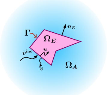
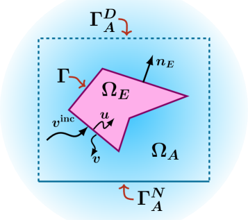
Figure 1: Schematic representation of the problem geometry. Left: The elastic domain $\Omega_{E}$ is bounded; its Lipschitz boundary is denoted as $\Gamma$. The domain $\Omega_{A}$ where the acoustic waves propagate is unbounded. Right: An artificial boundary $\Gamma_{A}$ enclosing the elastic domain is introduced. The artificial boundary is split onto two disjoint components $\Gamma_{A}^{D}$ and $\Gamma_{A}^{N}$ where Dirichlet and Neumann boundary conditions are imposed respectively.

When viewed in full generality, the acoustic propagation region $\Omega_{A}$ is in fact unbounded and given by $\Omega_{A}:=\mathbb{R}^{n}\setminus\overline{\Omega_{E}}$. This fact introduces further computational challenges that are often addressed either through an integral equation representation of the acoustic wave BrSaSa:2016 ; HsSa:2021 ; HsSaSa:2016 ; SV:2024 , the introduction of a perfectly matched layer LiTa:1997 , the use of absorbing boundary conditions EnMa:1977 ; HaTr:1988 ; Hi:1987 ; HaTr:1986 or the representation of the acoustic field through a moment expansion AlAn:2024 .

In this communication, we simplify the analysis by introducing an artificial boundary that will allow us to assume that the acoustic domain is in fact bounded. As depicted in the right panel of Figure 1, we pick a polygon with boundary $\Gamma_{A}$ (the subscript standing for “artificial”) that compactly contains the elastic domain $\Omega_{E}$. The boundary $\Gamma_{A}$ is divided into mutually disjoint Dirichlet and Neumann segments (denoted respectively by $\Gamma_{A}^{D}$ and $\Gamma_{A}^{N}$) such that $\Gamma_{A}=\Gamma_{A}^{D}\cup\Gamma_{A}^{N}$. The acoustic domain $\Omega_{A}$ is then defined to be the region exterior to $\Omega_{E}$ and contained inside the polygon. Its boundary takes the form

$$\partial\Omega_{A}:=\Gamma\cup\Gamma_{A}^{D}\cup\Gamma_{A}^{N}$$

where the three components are mutually disjoint and $\Gamma$ denotes the interface between the acoustic and elastic regions. We emphasize that the boundary conditions imposed on $\Gamma_{A}$ do not attempt to account for a physically outgoing wave, but simply to ensure the well-posedness of the simplified problem. The goal of this work is to establish the well-posedness theory for the coupling of HDG discretizations for elastic and acoustic wave propagation. The treatment of the fully unbounded problem will be the subject of a separate communication.

Assuming that at the initial time the incident wave $v^{\text{inc}}$ is supported away from the elastic domain $\Omega_{E}$, the distributional version of the system above admits a Laplace transform HsSaSa:2016 that maps time differentiation to multiplication by the Laplace parameter $s\in\{z\in\mathbb{C}:\mathrm{Re}\!\left(z\right)>0\}$. Upon Laplace transformation and using the same symbols for the unknowns in the time domain and in the Laplace domain, the elastic wave $\bm{u}$ and the scattered acoustic wave $v$ satisfy the coupled system of equations in mixed form

$$\mathbf{C}^{-1}\bm{\sigma}-\nabla\bm{u}+\bm{\gamma} =\bm{0} \text{ in }\Omega_{E},$$ (1a)

$$-\nabla\hskip-1.42271pt\cdot\bm{\sigma}+\rho_{E}s^{2}\bm{u} =\bm{f} \text{ in }\Omega_{E},$$ (1b)

$$\bm{q}-\nabla v =\bm{0} \text{ in }\Omega_{A},$$ (1c)

$$-\nabla\hskip-1.42271pt\cdot\bm{q}+(s/c)^{2}v =f\hskip 14.22636pt \text{ in }\Omega_{A},$$ (1d)

$$\bm{q}\cdot\bm{n}_{A}-s\,\bm{u}\cdot\bm{n}_{E} =-\nabla v^{\text{inc}}\cdot\bm{n}_{A} \text{ on }\Gamma,$$ (1e)

$$-\bm{\sigma}\bm{n}_{E}+\rho_{f}s\,v\,\bm{n}_{A} =-\rho_{f}s\,v^{\text{inc}}\,\bm{n}_{A} \text{ on }\Gamma,$$ (1f)

$$v =g_{D} \text{ on }\Gamma_{A}^{D},$$ (1g)

$$\bm{q}\cdot\bm{n}_{A} =g_{N} \text{ on }\Gamma_{A}^{N}.$$ (1h)

Here, $\bm{q}$ is the acoustic velocity field, and $g_{D}\in H^{1/2}(\Gamma_{A}^{D})$ and $g_{N}\in H^{-1/2}(\Gamma_{A}^{N})$ are given boundary data.

In the system above, equations (1a) and (1b) account for the Navier-Lamé or elastic wave equation in the interior of the elastic solid $\Omega_{E}$. Similarly, equations (1c) and (1d) are the mixed form of the acoustic wave equation in $\Omega_{A}$. The elastic and acoustic variables are coupled through the continuity of the normal component of the velocity field across the interface $\Gamma$, encoded in equation (1e), and the balance of normal forces at the contact surface, given in (1f). The nonphysical boundary conditions (1g) and (1h) prescribed at the artificial boundary $\Gamma_{A}$ are given to ensure the well-posedness of the problem.

In the literature, there is a vast amount of research related to fluid-structure interaction problems. For instance, some of them use a Mixed Finite Elements approach DoGaMe:2015 ; GaMaMe:2012 and there are also couplings of this technique with Boundary Element Methods GaHeMe:2014 . Studies on their spectral problems MeMoRo:2014 and an analysis of the elastoacustic problem in the time domain ArRoVe:2019 have been done. However, most of these works assume a time-harmonic regime, while we intend to focus on the transient regime. Moreover, since two different systems of PDEs posed in different domains are being coupled across an interface, we prefer to use a discontinuous Galerkin scheme due to its flexibility to handle the transmission conditions. In particular, by considering the HDG method introduced in CoGoLa2009 , it is very easy to impose transmission conditions from the computational point of view. In fact, in HDG schemes the only globally coupled degrees of freedom are precisely those of the numerical traces on the boundaries between elements, while the remaining unknowns are obtained by solving local problems in each element. Therefore, if we have two independent HDG solvers, one for the acoustic problem and another one for the elastic system, we can couple them across the interface through the numerical traces associated with the acoustic wave $v$ and the elastic displacements $\bm{u}$.

After CoGoLa2009 and the pioneering work CoGoSa2010 that set a framework that simplifies the analysis of a family of HDG schemes by introducing a suitable projection, HDG schemes have been developed for a wide variety of problems. For example, convection-diffusion equation FuQiZh2015 ; NgPeCo2009 , Stokes flow CoGoNgPe2011 ; GaSe2016 ; Brinkman, Oseen and Navier–Stokes equations CeCoNgPe2013 ; CeCoQi2017 ; FuJiQi2016 ; NgPeCo2011NS . In the context of electromagnetism and wave propagation problems, HDG schemes have also been introduced: Maxwell’s operator ChQiSh2018 ; ChQiShSo2017 , eddy current problems BuLoOs2018 , Maxwell’s equations in the frequency-domain FePeXu2016 ; NgPeCo2011 and heterogeneous media CaLoOsSo2020 and Helmholtz equation ChPeXu2013 ; GrMo2011 ; ZhWu2021 , and even for nonlinear problems arising from plasma physics SaSaSo:2021a ; SaSaSo:2019 ; SaSo:2018 ; SaSoCe:2018 . For the elasticity problem, we refer the reader to Ke ; QiShSh2018 . The preceding list of references is not exhaustive, but provides an overview of the development of HDG schemes during the last fifteen years.

On the other hand, in the context of coupled problems with piecewise linear interfaces, HDG schemes have been proposed for elliptic Huynh2013 and for the Stokes interface problems Wang2013HDG , and for Stokes-Darcy coupling GaSe2017 . The influence of hanging-nodes along the interface and the use of different polynomial degree over each local space, have been analyzed in Chen2012 ; Chen2013 . Recently, a new approach has been proposed to handle discrete interfaces that not necessarily coincides with the true interface, as in the case of a curved interface BeMaSo2025 ; MaNgSo2022 ; SoTeNgPe2022 and it is based on the Transfer Path Method CoQiSo2014 ; CoSo2012 ; SaSaSo2022 . This technique produces a high order method and is closely related with our ultimate goal, where it is crucial to have a numerical scheme that couples an HDG discretization of the problem posed in an bounded domain considering a solid with a curved boundary, and a representation of the acoustic wave in the unbounded region. To the best of our knowledge, the use of HDG schemes has not been analyzed for the coupled problem (1), and the main contribution of this work is to provide a convergence analysis.

2 Preliminaries and notation

2.1 Sobolev spaces.

Let $\mathcal{O}$ be a Lipschitz continuous domain in $\mathbb{R}^{n}$. We use standard notations for Lebesgue $\mathrm{L}^{t}(\mathcal{O})$ and Sobolev spaces $\mathrm{W}^{l,t}(\mathcal{O})$, with $l\,\geq\,0$ and $t\in[1,+\infty)$. Here $\mathrm{W}^{0,t}(\mathcal{O})\,=\,\mathrm{L}^{t}(\mathcal{O})$, and if $t\,=\,2$ we write $\mathrm{H}^{l}(\mathcal{O})$ instead of $\mathrm{W}^{l,2}(\mathcal{O})$, with the corresponding norm and seminorm denoted by $\|\cdot\|_{H^{l}(\mathcal{O})}$ and $|\cdot|_{H^{l}(\mathcal{O})}$, respectively. The spaces of vector-valued functions will be denoted in boldface, therefore $\bm{H}^{s}(\mathcal{O}):=[H^{s}(\mathcal{O})]^{n}$, whereas for tensor-valued functions, we write $\underline{\bm{H}}^{s}(\mathcal{O}):=[H^{s}(\mathcal{O})]^{n\times n}$. Using the same notation, we write $\bm{L}^{2}(\mathcal{O}):=[L^{2}(\mathcal{O})]^{n}$ and $\underline{\bm{L}}^{2}(\mathcal{O}):=[L^{2}(\mathcal{O})]^{n\times n}.$

The complex $L^{2}$-inner products will be denoted by $(\cdot,\cdot)_{\mathcal{O}}$ and $\langle\cdot,\cdot\rangle_{\Sigma}$, where $\Sigma$ is either a Lipschitz curve ($n=2$) or a surface ($n=3$). The associated norms will be denoted by $\|\cdot\|_{\mathcal{O}}$ and $\|\cdot\|_{\Sigma}$.

It is easy to verify that Hooke’s tensor satisfies the following inequalities for all $\bm{\eta}\in\underline{\bm{L}}^{2}(\mathcal{O})$:

$$\left(\dfrac{1}{2\mu}+\dfrac{n^{2}\lambda}{2\mu(n\lambda+2\mu)}\right)^{-1}\|\bm{\eta}\|_{\mathcal{O},\mathbf{C}^{-1}}^{2} \leq\|\bm{\eta}\|^{2}_{\mathcal{O}}\leq 2\mu\|\bm{\eta}\|_{\mathcal{O},\mathbf{C}^{-1}}^{2},$$

$$\|\bm{\eta}\|_{\mathcal{O},\mathbf{C}}^{2} \leq(2\mu+n^{2}\lambda)\|\bm{\eta}\|^{2}_{\mathcal{O}},$$

where we denote $\|\cdot\|_{\mathcal{O},\mathbf{C}^{-1}}:=(\mathbf{C}^{-1}\cdot,\cdot)_{\mathcal{O}}^{1/2}$ and $\|\cdot\|_{\mathcal{O},\mathbf{C}}:=(\mathbf{C}\cdot,\cdot)_{\mathcal{O}}^{1/2}$.

2.2 Mesh and mesh-dependent inner products.

Let $\mathcal{T}_{A}$ and $\mathcal{T}_{E}$ be two families of regular triangulations of $\Omega_{A}$ and $\Omega_{E}$, respectively. We will assume that these triangulations are compatible along the common interface $\Gamma$ and that both are characterized by a common mesh size $h$ in their respective domains. Given an element $K$, $h_{K}$ will denote its diameter and $\bm{n}_{K}$ its outward unit normal. When there is no confusion, we will simply write $\bm{n}$ instead of $\bm{n}_{K}$. Set $\dagger\in\{A,E\}$, then $\partial\mathcal{T}_{\dagger}:=\{\partial K:K\in\mathcal{T}_{\dagger}\}$ and let $\mathcal{E}_{\dagger}$ denote the set of all faces $F$ of all elements $K\in\mathcal{T}_{\dagger}$. We will also use the following notation for $L^{2}$ inner products of scalar-, vector- and tensor-valued functions, respectively, over an integration domain $D$:

$$(u,v)_{D}:=\int_{D}u\overline{v},\qquad(\bm{u},\bm{v})_{D}=\int_{D}\bm{u}\cdot\overline{\bm{v}},\qquad(\bm{M},\bm{N})_{D}=\int_{D}\bm{M}:\overline{\bm{N}},$$

where the overline denotes complex conjugation and the colon “$\,:\,$” is used to denote the Frobenius inner product of matrices

$$\bm{M}:\bm{N}:=\sum_{i,j=1}^{n}M_{ij}N_{ij}.$$

With this notation we can express the mesh-dependent $L^{2}$ inner products as

$$\left(u,v\right)_{\mathcal{T}_{\dagger}}:=\displaystyle\sum_{K\in\mathcal{T}_{\dagger}}\left(u,v\right)_{K},\left(\bm{u},\bm{v}\right)_{\mathcal{T}_{\dagger}}:=\displaystyle\sum_{K\in\mathcal{T}_{\dagger}}\left(\bm{u},\bm{v}\right)_{K},\quad\left(\bm{M},\bm{N}\right)_{\mathcal{T}_{\dagger}}:=\displaystyle\sum_{K\in\mathcal{T}_{\dagger}}\left(\bm{M},\bm{N}\right)_{K},$$

along with the inner products over the mesh skeleton

$$\langle u,v\rangle_{\partial\mathcal{T}_{\dagger}}:=\!\displaystyle\sum_{K\in\mathcal{T}_{\dagger}}\!\left\langle u,v\right\rangle_{\partial K},\langle\bm{u},\bm{v}\rangle_{\partial\mathcal{T}_{\dagger}}:=\!\displaystyle\sum_{K\in\mathcal{T}_{\dagger}}\!\left\langle\bm{u},\bm{v}\right\rangle_{\partial K},\langle\bm{M},\bm{N}\rangle_{\partial\mathcal{T}_{\dagger}}:=\!\displaystyle\sum_{K\in\mathcal{T}_{\dagger}}\!\left\langle\bm{M},\bm{N}\right\rangle_{\partial K}.$$

We denote the norms induced by these inner products by

$$\|\cdot\|_{\mathcal{T}_{\dagger}}:=\sqrt{\left(\cdot,\cdot\right)_{\mathcal{T}_{\dagger}}}\qquad\text{ and }\qquad\|\cdot\|_{\partial\mathcal{T}_{\dagger}}:=\sqrt{\langle\cdot,\cdot\rangle_{\partial\mathcal{T}_{\dagger}}}.$$

Finally, to avoid proliferation of superflous constants, we will write $a\lesssim b$ when there exists a positive constant $C$, independent of the mesh size, such that $a\leq Cb$.

2.3 The HDG polynomial spaces

We will make use of the discrete spaces for the HDG method proposed in Ke for simplices. For an element $K\in\mathcal{T}_{A}\cup\mathcal{T}_{E}$, we define the following function spaces. The set of scalar-valued polynomials of degree at most $k$ defined over $K$ will be denoted by $\mathcal{P}_{k}\!\left(K\right)$, while the corresponding vector and tensor product spaces are denoted respectively as

$$\bm{\mathcal{P}}_{k}\!\left(K\right):=[\mathcal{P}_{k}\!\left(K\right)]^{n}\qquad\text{ and }\qquad\underline{\bm{\mathcal{P}}}_{k}\!\left(K\right):=[\mathcal{P}_{k}\!\left(K\right)]^{n\times n}.$$

The polynomial spaces of degree exactly $k$ will be denoted with a tilde as $\widetilde{\mathcal{P}}_{k}(K)$, $\widetilde{\bm{\mathcal{P}}}_{k}(K)$, and $\widetilde{\underline{\bm{\mathcal{P}}}}_{k}(K)$. We now define

$$A_{ij}\left(K\right):=\begin{cases}\mathcal{P}_{k}\!\left(K\right)&\text{if}\hskip 8.5359pti\neq j,\\ 0&\text{if}\hskip 8.5359pti=j,\end{cases},$$

and use it to construct the matrix-valued space

$$\underline{\bm{A}}\!\left(K\right):=[A_{ij}\left(K\right)]^{n\times n}.$$

We will denote the space of $L^{2}$ integrable skew-symmetric matrices over $K$ by

$$\underline{\bm{AS}}\!\left(K\right):=\{{\bm{M}}\in\underline{\bm{L}}^{2}\!\left(K\right):{\bm{M}}+{\bm{M}}^{\top}={\bm{0}}\},$$

and will require that $\underline{\bm{A}}\!\left(K\right)\subset\underline{\bm{AS}}\!\left(K\right)$.

Now, we would like to define a divergence-free space of functions through the use of bubble matrices or bubble scalars, depending on the dimension, as in CaSo:2023 ; CoGoGu:2009 ; Ke ; Gu:2010 . Following Gu:2010 , a matrix-valued function $\bm{b}$ defined in $\Omega_{E}$ is said to be an admissible bubble matrix if for each $K\in\mathcal{T}_{E}$ the matrix $\bm{b}_{K}:=\left.\bm{b}\right|_{K}$ is a matrix with polynomial entries that satisfies

1. The tangential components of each row of $\bm{b}_{K}$ vanish on all the faces of $K$,

2. There exists $C_{1}>0$ such that $C_{1}(\bm{v},\bm{v})_{K}\leq(\bm{vb}_{K},\bm{v})_{K}$, for all $\bm{v}\in\underline{\bm{L}}^{2}(K)$,

3. There exists $C_{2}>0$ such that $\|\bm{b}_{K}\|_{\underline{\bm{L}}^{\infty}(K)}\leq C_{2}$,

where the constants $C_{1}$ and $C_{2}$ depend only on the shape regularity of $\mathcal{T}_{E}$.

Thus, following CoGoGu:2009 ; Ke , if $\eta_{F}$ is the barycentric coordinate associated to the edge $F$ of $K$, and if we define

$$\bm{b}_{K}:={\begin{cases}\displaystyle\prod_{F\subset\partial K}\eta_{F}&\text{in 2D },\\[4.30554pt] \displaystyle\sum_{F\subset\partial K}\left[\displaystyle\prod_{F^{\prime}\subset\partial K\setminus\{F\}}\eta_{F^{\prime}}\right]\nabla\eta_{F}\otimes\nabla\eta_{F}&\text{in 3D},\end{cases}}$$

the polynomial space $\underline{\bm{B}}\!\left(K\right)$ associated to bubble functions is defined as:

$$\underline{\bm{B}}\!\left(K\right):=\nabla\times((\nabla\times\underline{\bm{A}}\!\left(K\right))\bm{b}_{K}).$$

We can observe that any function

$$\bm{v}\in\underline{\bm{\mathcal{B}}}_{h}:=\{\bm{\eta}\in\underline{\bm{L}}^{2}(\Omega_{E}):\left.\bm{\eta}\right|_{K}\in\underline{\bm{B}}\!\left(K\right),K\in\mathcal{T}_{E}\}$$

is such that

$$\left.\nabla\hskip-1.42271pt\cdot\bm{v}\right|_{K}=0,\forall\,K\in\mathcal{T}_{E}\quad\text{ and }\quad\left.\bm{v}\bm{n}\right|_{F}=0,\forall F\in\mathcal{E}_{E}.$$

In the three-dimensional case the curl operator acts row-wise, while in the two-dimensional case the curl of matrices and column vectors are defined respectively by

$$\nabla\times\begin{pmatrix}M_{11}&M_{12}\\ M_{21}&M_{22}\end{pmatrix}:=\begin{pmatrix}\partial_{x}M_{12}-\partial_{y}M_{11}\\ \partial_{x}M_{22}-\partial_{y}M_{21}\end{pmatrix}\quad\text{and}\quad\nabla\times\begin{pmatrix}m_{1}\\ m_{2}\end{pmatrix}:=\begin{pmatrix}-\partial_{y}m_{1}&\partial_{x}m_{1}\\ -\partial_{y}m_{2}&\partial_{x}m_{2}\end{pmatrix}$$

We will also make use of the local space $\underline{\bm{V}}\!\left(K\right):=\underline{\bm{\mathcal{P}}}_{k}\!\left(K\right)+\underline{\bm{B}}\!\left(K\right)$, and notice that

$$\underline{\bm{V}}\!\left(K\right)=\underline{\bm{\mathcal{P}}}_{k}\!\left(K\right)+\nabla\times((\nabla\times\underline{\bm{A}}\!\left(K\right))\bm{b}_{K})=\underline{\bm{\mathcal{P}}}_{k}\!\left(K\right)\oplus\nabla\times((\nabla\times\underline{\bm{\widetilde{A}}}\!\left(K\right))\bm{b}_{K}),$$

where $\underline{\bm{\widetilde{A}}}\!\left(K\right):=\underline{\bm{A}}\!\left(K\right)\cap\underline{\bm{\widetilde{\mathcal{P}}}}_{k}\!\left(K\right)$.

3 An HDG discretization

Let us begin by introducing the piecewise polynomial spaces

$$\underline{\bm{V}}_{h} =\{\bm{\tau}\in\underline{\bm{L}}^{2}\!\left(\mathcal{T}_{E}\right):\left.\bm{\tau}\right|_{K}\in\underline{\bm{V}}\!\left(K\right),\hskip 8.5359pt\forall K\in\mathcal{T}_{E}\},$$ (2a)

$$\bm{W}_{h}^{E} =\{\bm{t}\in\bm{L}^{2}\!\left(\mathcal{T}_{E}\right):\left.\bm{t}\right|_{K}\in\bm{\mathcal{P}}_{k}\!\left(K\right),\hskip 8.5359pt\forall K\in\mathcal{T}_{E}\},$$ (2b)

$$\underline{\bm{A}}_{h} =\{\bm{\eta}\in\underline{\bm{L}}^{2}\!\left(\mathcal{T}_{E}\right):\left.\bm{\eta}\right|_{K}\in\underline{\bm{A}}\!\left(K\right),\hskip 8.5359pt\forall K\in\mathcal{T}_{E}\},$$ (2c)

$$\bm{M}_{h} =\{\bm{\mu}\in\bm{L}^{2}\!\left(\mathcal{E}_{E}\right):\left.\bm{\mu}\right|_{F}\in\bm{\mathcal{P}}_{k}\!\left(F\right),\hskip 8.5359pt\forall F\in\mathcal{E}_{E}\},$$ (2d)

$$\bm{W}_{h}^{A} =\{\bm{r}\in\bm{L}^{2}\!\left(\mathcal{T}_{A}\right):\left.\bm{r}\right|_{K}\in\bm{\mathcal{P}}_{k}\!\left(K\right),\hskip 8.5359pt\forall K\in\mathcal{T}_{A}\},$$ (2e)

$$W_{h} =\{w\in L^{2}\!\left(\mathcal{T}_{A}\right):\left.w\right|_{K}\in\mathcal{P}_{k}\!\left(K\right),\hskip 8.5359pt\forall K\in\mathcal{T}_{A}\},$$ (2f)

$$M_{h} =\{\xi\in L^{2}\!\left(\mathcal{E}_{A}\right):\left.\xi\right|_{F}\in\mathcal{P}_{k}\!\left(F\right),\hskip 8.5359pt\forall F\in\mathcal{E}_{A}\}.$$ (2g)

The HDG discretization seeks a piecewise polynomial approximation

$$(\bm{\sigma}_{h},\bm{u}_{h},\bm{\gamma}_{h},\widehat{\bm{u}}_{h},\bm{q}_{h},v_{h},\widehat{v}_{h})\in\underline{\bm{V}}_{h}\times\bm{W}_{h}^{E}\times\underline{\bm{A}}_{h}\times\bm{M}_{h}\times\bm{W}_{h}^{A}\times W_{h}\times M_{h}$$

of the exact solution $(\bm{\sigma},\bm{u},\bm{\gamma},\left.\bm{u}\right|_{\mathcal{E}_{E}},\bm{q},v,\left.v\right|_{\mathcal{E}_{A}})$. The approximation must satisfy the discrete weak formulation

$$(\mathbf{C}^{-1}\bm{\sigma}_{h},\bm{\tau})_{\mathcal{T}_{E}}+(\bm{u}_{h},\nabla\hskip-1.42271pt\cdot\bm{\tau})_{\mathcal{T}_{E}}+(\bm{\gamma}_{h},\bm{\tau})_{\mathcal{T}_{E}}-\langle\widehat{\bm{u}}_{h},\bm{\tau}\bm{n}\rangle_{\partial\mathcal{T}_{E}} =0,$$ (3a)

$$(\bm{\sigma}_{h},\nabla\bm{t})_{\mathcal{T}_{E}}-\langle\widehat{\bm{\sigma}}_{h}\bm{n},\bm{t}\rangle_{\partial\mathcal{T}_{E}}+\rho_{E}s^{2}(\bm{u}_{h},\bm{t})_{\mathcal{T}_{E}} =(\bm{f},\bm{t})_{\mathcal{T}_{E}},$$ (3b)

$$(\bm{\sigma}_{h},\bm{\eta})_{\mathcal{T}_{E}} =0,$$ (3c)

$$\langle\widehat{\bm{\sigma}}_{h}\bm{n},\bm{\mu}\rangle_{\partial\mathcal{T}_{E}\setminus\Gamma} =0,$$ (3d)

$$(\bm{q}_{h},\bm{r})_{\mathcal{T}_{A}}+(v_{h},\nabla\hskip-1.42271pt\cdot\bm{r})_{\mathcal{T}_{A}}-\langle\widehat{v}_{h},\bm{r}\cdot\bm{n}\rangle_{\partial\mathcal{T}_{A}} =0,$$ (3e)

$$(\bm{q}_{h},\nabla w)_{\mathcal{T}_{A}}-\langle\widehat{\bm{q}}_{h}\cdot\bm{n},w\rangle_{\partial\mathcal{T}_{A}}+(s/c)^{2}(v_{h},w)_{\mathcal{T}_{A}} =(f,w)_{\mathcal{T}_{A}},$$ (3f)

$$\langle\widehat{\bm{q}}_{h}\cdot\bm{n},\xi\rangle_{\partial\mathcal{T}_{A}\setminus(\Gamma\cup\Gamma_{A}^{D})} =\langle g_{N},\xi\rangle_{\Gamma_{A}^{N}},$$ (3g)

$$\langle\widehat{v}_{h},\xi\rangle_{\Gamma_{A}^{D}} =\langle g_{D},\xi\rangle_{\Gamma_{A}^{D}},$$ (3h)

$$\langle\widehat{\bm{q}}_{h}\cdot\bm{n}_{A}-s\,\widehat{\bm{u}}_{h}\cdot\bm{n}_{E},\xi\rangle_{\Gamma} =-\langle\nabla v^{\text{inc}}\cdot\bm{n}_{A},\xi\rangle_{\Gamma},$$ (3i)

$$\langle-\widehat{\bm{\sigma}}_{h}\bm{n}_{E}+\rho_{f}s\,\widehat{v}_{h}\,\bm{n}_{A},\bm{\mu}\rangle_{\Gamma} =-\rho_{f}s\,\langle v^{\text{inc}}\,\bm{n}_{A},\bm{\mu}\rangle_{\Gamma}$$ (3j)

for all test functions $$(\bm{\tau},\bm{t},\bm{\eta},\bm{\mu},\bm{r},w,\xi)\in\underline{\bm{V}}_{h}\times\bm{W}_{h}^{E}\times\underline{\bm{A}}_{h}\times\bm{M}_{h}\times\bm{W}_{h}^{A}\times W_{h}\times M_{h}$$, where

$$\widehat{\bm{\sigma}}_{h}\bm{n} :=\bm{\sigma}_{h}\bm{n}-\tau_{E}(\bm{u}_{h}-\widehat{\bm{u}}_{h})\hskip 28.45274pt\text{on}\hskip 14.22636pt\partial\mathcal{T}_{E},$$ (3k)

$$\widehat{\bm{q}}_{h}\cdot\bm{n} :=\bm{q}_{h}\cdot\bm{n}-\tau_{A}(v_{h}-\widehat{v}_{h})\hskip 28.45274pt\text{on}\hskip 14.22636pt\partial\mathcal{T}_{A}.$$ (3l)

Here, $$\tau_{E} \tau_{A}$$ and are stabilization parameters whose properties will be determined when analyzing the scheme.

4 Discrete well posedness.

Theorem 4.1

If $\mathrm{Re}\!\left(s\tau_{A}\right)>0$ and $\mathrm{Re}\!\left(s\tau_{E}\right)>0$, then the scheme (3) has a unique solution.

Proof

By the Fredholm alternative, it is enough to show uniqueness of the solution. To that end, if we assume zero sources, we will show that the solution to the corresponding system is the trivial one.

Let

$$v^{\text{inc}}=0\qquad\text{ and }\qquad(f,\bm{f},g_{D},g_{N})=(0,\bm{0},0,0),$$

and choose

$$(\bm{\tau},\bm{t},\bm{\eta},\bm{\mu},\bm{r},w)=(\widehat{\bm{\sigma}}_{h},\bm{u}_{h},\bm{\gamma}_{h},\widehat{\bm{u}}_{h},\bm{q}_{h},v_{h})\qquad\text{ and }\qquad\xi=\left\{\begin{array}[]{rl}\widehat{v}_{h},&\text{on }\partial\mathcal{T}_{A}\setminus\Gamma_{A}^{D}\\ \widehat{\bm{q}}_{h}\cdot\bm{n},&\text{on }\Gamma_{A}^{D}\\ \end{array}\right.\,.$$

With this choice of test functions, applying integration by parts to (3b) and adding its conjugate to (3a) we obtain

$$(\mathbf{C}^{-1}\bm{\sigma}_{h},\bm{\sigma}_{h})_{\mathcal{T}_{E}}+(\bm{u}_{h},\nabla\hskip-1.42271pt\cdot\bm{\sigma}_{h})_{\mathcal{T}_{E}}+(\bm{\gamma}_{h},\bm{\sigma}_{h})_{\mathcal{T}_{E}}-\langle\widehat{\bm{u}}_{h},\bm{\sigma}_{h}\bm{n}\rangle_{\partial\mathcal{T}_{E}}$$

$$-\overline{(\nabla\hskip-1.42271pt\cdot\bm{\sigma}_{h},\bm{u}_{h})_{\mathcal{T}_{E}}}+\overline{\langle\bm{\sigma}_{h}\bm{n},\bm{u}_{h}\rangle_{\partial\mathcal{T}_{E}}}-\overline{\langle\widehat{\bm{\sigma}}_{h}\bm{n},\bm{u}_{h}\rangle_{\partial\mathcal{T}_{E}}}+\rho_{E}\overline{s^{2}}(\bm{u}_{h},\bm{u}_{h})_{\mathcal{T}_{E}}=0.$$

We know from (3c) that $(\bm{\sigma}_{h},\bm{\gamma}_{h})_{\mathcal{T}_{E}}=0$, so the latter equation becomes

$$(\mathbf{C}^{-1}\bm{\sigma}_{h},\bm{\sigma}_{h})_{\mathcal{T}_{E}}+\overline{\langle\bm{\sigma}_{h}\bm{n}-\widehat{\bm{\sigma}}_{h}\bm{n},\bm{u}_{h}\rangle_{\partial\mathcal{T}_{E}}}-\langle\widehat{\bm{u}}_{h},\bm{\sigma}_{h}\bm{n}\rangle_{\partial\mathcal{T}_{E}}+\rho_{E}\overline{s^{2}}(\bm{u}_{h},\bm{u}_{h})_{\mathcal{T}_{E}}=0.$$

Adding and subtracting $\widehat{\bm{u}}_{h}$ in the second argument of the second term, we have that

$$\left\|\bm{\sigma}_{h}\right\|_{\mathcal{T}_{E},\mathbf{C}^{-1}}^{2} +\overline{\langle\bm{\sigma}_{h}\bm{n}-\widehat{\bm{\sigma}}_{h}\bm{n},\bm{u}_{h}-\widehat{\bm{u}}_{h}\rangle_{\partial\mathcal{T}_{E}}}+\overline{\langle\bm{\sigma}_{h}\bm{n}-\widehat{\bm{\sigma}}_{h}\bm{n},\widehat{\bm{u}}_{h}\rangle_{\partial\mathcal{T}_{E}}}$$

$$-\langle\widehat{\bm{u}}_{h},\bm{\sigma}_{h}\bm{n}\rangle_{\partial\mathcal{T}_{E}}+\rho_{E}\overline{s^{2}}\left\|\bm{u}_{h}\right\|_{\mathcal{T}_{E}}^{2}=0.$$

Multiplying by $s$ and using (3d), along with the definition (3k), we obtain

$$s\left\|\bm{\sigma}_{h}\right\|_{\mathcal{T}_{E},\mathbf{C}^{-1}}^{2}+s\overline{\langle\tau_{E}(\bm{u}_{h}-\widehat{\bm{u}}_{h}),\bm{u}_{h}-\widehat{\bm{u}}_{h}\rangle_{\partial\mathcal{T}_{E}}}-s\langle\widehat{\bm{u}}_{h},\widehat{\bm{\sigma}}_{h}\bm{n}_{E}\rangle_{\Gamma}+\rho_{E}\overline{s}|s|^{2}\left\|\bm{u}_{h}\right\|_{\mathcal{T}_{E}}^{2}=0.$$ (4)

Analogously for the acoustic terms, (3f) is integrated by parts and its conjugate is added to (3e), yielding

$$\left\|\bm{q}_{h}\right\|_{\mathcal{T}_{A}}^{2}+ (v_{h},\nabla\hskip-1.42271pt\cdot\bm{q}_{h})_{\mathcal{T}_{A}}-\langle v_{h},\bm{q}_{h}\cdot\bm{n}\rangle_{\partial\mathcal{T}_{A}}-\overline{(\nabla\hskip-1.42271pt\cdot\bm{q}_{h},v_{h})_{\mathcal{T}_{A}}}$$

$$+\overline{\langle\bm{q}_{h}\cdot\bm{n},v_{h}\rangle_{\partial\mathcal{T}_{A}}}-\overline{\langle\widehat{\bm{q}}_{h}\cdot\bm{n},v_{h}\rangle_{\partial\mathcal{T}_{A}}}+\frac{\overline{s^{2}}}{c^{2}}\left\|v_{h}\right\|_{\mathcal{T}_{A}}^{2}=0.$$

Adding and subtracting $\widehat{v}_{h}$ and using (3g) and (3h), we can deduce that

$$\left\|\bm{q}_{h}\right\|_{\mathcal{T}_{A}}^{2}+\overline{\langle\tau_{A}(v_{h}-\widehat{v}_{h}),v_{h}-\widehat{v}_{h}\rangle_{\partial\mathcal{T}_{A}}}-\langle\widehat{v}_{h},\widehat{\bm{q}}_{h}\cdot\bm{n}_{A}\rangle_{\Gamma}+\frac{\overline{s^{2}}}{c^{2}}\left\|v_{h}\right\|_{\mathcal{T}_{A}}^{2}=0.$$

We multiply the latter equation by $\rho_{f}s$ to obtain

$$\rho_{f}s\left\|\bm{q}_{h}\right\|_{\mathcal{T}_{A}}^{2}+\rho_{f}s\overline{\langle\tau_{A}(v_{h}-\widehat{v}_{h}),v_{h}-\widehat{v}_{h}\rangle_{\partial\mathcal{T}_{A}}}-\rho_{f}s\langle\widehat{v}_{h},\widehat{\bm{q}}_{h}\cdot\bm{n}_{A}\rangle_{\Gamma}+\rho_{f}\overline{s}(|s|/c)^{2}\left\|v_{h}\right\|_{\mathcal{T}_{A}}^{2}=0.$$ (5)

Adding (4) with the conjugate of (5) leads to

$$\begin{array}[]{l}\;\;\,s\left\|\bm{\sigma}_{h}\right\|_{\mathcal{T}_{E},\mathbf{C}^{-1}}^{2}+s\overline{\langle\tau_{E}(\bm{u}_{h}-\widehat{\bm{u}}_{h}),\bm{u}_{h}-\widehat{\bm{u}}_{h}\rangle_{\partial\mathcal{T}_{E}}}-s\langle\widehat{\bm{u}}_{h},\widehat{\bm{\sigma}}_{h}\bm{n}_{E}\rangle_{\Gamma}+\rho_{E}\overline{s}|s|^{2}\left\|\bm{u}_{h}\right\|_{\mathcal{T}_{E}}^{2}\\ +\rho_{f}\overline{s}\left\|\bm{q}_{h}\right\|_{\mathcal{T}_{A}}^{2}+\rho_{f}\overline{s}\langle\tau_{A}(v_{h}-\widehat{v}_{h}),v_{h}-\widehat{v}_{h}\rangle_{\partial\mathcal{T}_{A}}-\rho_{f}\overline{s}\overline{\langle\widehat{v}_{h},\widehat{\bm{q}}_{h}\cdot\bm{n}_{A}\rangle_{\Gamma}}+\rho_{f}\overline{s}(|s|/c)^{2}\left\|v_{h}\right\|_{\mathcal{T}_{A}}^{2}=0\end{array}$$ (6)

Notice that from (3i) and (3j) we have

$$-s\langle\widehat{\bm{u}}_{h},\widehat{\bm{\sigma}}_{h}\bm{n}_{E}\rangle_{\Gamma}-\rho_{f}\overline{s}\overline{\langle\widehat{v}_{h},\widehat{\bm{q}}_{h}\cdot\bm{n}_{A}\rangle_{\Gamma}}= -s\langle\widehat{\bm{u}}_{h},\widehat{\bm{\sigma}}_{h}\bm{n}_{E}-\rho_{f}s\widehat{v}_{h}\bm{n}_{A}\rangle_{\Gamma}-s\langle\widehat{\bm{u}}_{h},\rho_{f}s\widehat{v}_{h}\bm{n}_{A}\rangle_{\Gamma}$$

$$-\rho_{f}\overline{s}\overline{\langle\widehat{v}_{h},\widehat{\bm{q}}_{h}\cdot\bm{n}_{A}-s\widehat{\bm{u}}_{h}\cdot\bm{n}_{E}\rangle_{\Gamma}}-\rho_{f}\overline{s}\overline{\langle\widehat{v}_{h},s\widehat{\bm{u}}_{h}\cdot\bm{n}_{E}\rangle_{\Gamma}}$$

$$= -s\langle\widehat{\bm{u}}_{h},\rho_{f}s\widehat{v}_{h}\bm{n}_{A}\rangle_{\Gamma}-\rho_{f}\overline{s}\overline{\langle\widehat{v}_{h},s\widehat{\bm{u}}_{h}\cdot\bm{n}_{E}\rangle_{\Gamma}}$$

$$= -s\overline{s}\rho_{f}\langle\widehat{\bm{u}}_{h},\widehat{v}_{h}\bm{n}_{A}\rangle_{\Gamma}+s\overline{s}\rho_{f}\langle\widehat{\bm{u}}_{h},\widehat{v}_{h}\bm{n}_{A}\rangle_{\Gamma}=\;0.$$

So, (6) is equivalent to

$$s\left\|\bm{\sigma}_{h}\right\|_{\mathcal{T}_{E},\mathbf{C}^{-1}}^{2}+s\overline{\langle\tau_{E}(\bm{u}_{h}-\widehat{\bm{u}}_{h}),\bm{u}_{h}-\widehat{\bm{u}}_{h}\rangle_{\partial\mathcal{T}_{E}}}+\rho_{E}\overline{s}|s|^{2}\left\|\bm{u}_{h}\right\|_{\mathcal{T}_{E}}^{2}$$

$$+ \rho_{f}\overline{s}\left\|\bm{q}_{h}\right\|_{\mathcal{T}_{A}}^{2}+\rho_{f}\overline{s}\langle\tau_{A}(v_{h}-\widehat{v}_{h}),v_{h}-\widehat{v}_{h}\rangle_{\partial\mathcal{T}_{A}}+\rho_{f}s(|s|/c)^{2}\left\|v_{h}\right\|_{\mathcal{T}_{A}}^{2}=0.$$

Thus, taking real part of this expression, we obtain

$$\mathscr{E}_{E}^{2}+\mathscr{E}_{A}^{2}+\rho_{E}|s|^{2}\mathrm{Re}\!\left(s\right)\left\|\bm{u}_{h}\right\|_{\mathcal{T}_{E}}^{2}+\frac{\rho_{f}}{c^{2}}|s|^{2}\mathrm{Re}\!\left(s\right)\left\|v_{h}\right\|_{\mathcal{T}_{A}}^{2}=0\,,$$

where we have defined

$$\mathscr{E}_{E} :=\sqrt{\left\|\mathrm{Re}\!\left(s\right)^{1/2}\bm{\sigma}_{h}\right\|_{\mathcal{T}_{E},\mathbf{C}^{-1}}^{2}+\left\|\mathrm{Re}\!\left(s\tau_{E}\right)^{1/2}(\bm{u}_{h}-\widehat{\bm{u}}_{h})\right\|_{\partial\mathcal{T}_{E}}^{2}}$$

$$\mathscr{E}_{A} :=\sqrt{\left\|\rho_{f}^{1/2}\mathrm{Re}\!\left(s\right)^{1/2}\bm{q}_{h}\right\|_{\mathcal{T}_{A}}^{2}+\left\|\rho_{f}^{1/2}\mathrm{Re}\!\left(s\tau_{A}\right)^{1/2}(v_{h}-\widehat{v}_{h})\right\|_{\partial\mathcal{T}_{A}}^{2}}.$$

From here, we can conclude that $\bm{\sigma}_{h}=\bm{0}$ in $\mathcal{T}_{E}$, $\bm{u}_{h}=\bm{0}$ in $\mathcal{T}_{E}$, $\bm{q}_{h}=\bm{0}$ in $\mathcal{T}_{A}$, $v_{h}=0$ in $\mathcal{T}_{A}$, $\widehat{\bm{u}}_{h}=\bm{u}_{h}=\bm{0}$ on $\partial\mathcal{T}_{E}$ and $\widehat{v}_{h}=v_{h}=0$ on $\partial\mathcal{T}_{A}$.

It only remains to show that $\bm{\gamma}_{h}=\bm{0}$ in $\mathcal{T}_{E}$. This will be achieved by performing an analog of the steps done in the proof of (CaSo:2023, , Lemma 3.6). We will need the two following technical results proven in Gu:2010 :

1. (Gu:2010, , Lemma 2.8) Given $\bm{\eta}\in\underline{\bm{A}}^{0}_{h}:=\{\bm{\eta}\in\underline{\bm{A}}_{h}:(\bm{\eta},\bm{v})_{K}=0,\forall\bm{v}\in\underline{\bm{\mathcal{P}}}_{0}\!\left(K\right),\forall K\in\mathcal{T}_{E}\}$, there exists $\bm{v}\in\underline{\bm{\mathcal{B}}}_{h}$ such that

   $$\bm{P}\bm{v}=\bm{\eta}\quad\text{ and }\quad\left\|\bm{v}\right\|_{\mathcal{T}_{E}}\leq C^{0}\left\|\bm{\eta}\right\|_{\mathcal{T}_{E}}.$$

   Here $\bm{P}:\underline{\bm{L}}^{2}\!\left(\Omega_{E}\right)\to\underline{\bm{A}}_{h}$ is the $L^{2}$-projection onto $\underline{\bm{A}}_{h}$ and $C^{0}$ is a positive constant independent of $h$, arising from a Poincaré-type inequality and inverse estimates.

2. (Gu:2010, , Proposition 2.9) Given $\bm{\eta}\in\underline{\bm{A}}^{c}_{h}:=\underline{\bm{A}}_{h}\cap\underline{\bm{\mathcal{P}}}_{0}\!\left(\mathcal{T}_{E}\right)$, there exists $\bm{v}\in\underline{\bm{H}}(\text{div};\Omega_{E})\cap\underline{\bm{\mathcal{P}}}_{1}\!\left(\mathcal{T}_{E}\right)$ such that

   $$\nabla\hskip-1.42271pt\cdot\bm{v}=0\,,\qquad\bm{P}^{c}\bm{v}=\bm{\eta}\,,\qquad\text{ and }\qquad\left\|\bm{v}\right\|_{\mathcal{T}_{E}}=C^{c}\left\|\bm{\eta}\right\|_{\mathcal{T}_{E}}\,,$$ (7)

   where $\bm{P}^{c}$ is the $L^{2}$-projection onto $\underline{\bm{A}}^{c}_{h}$, and $C^{c}>0$ is a constant independent of $h$.

Let us consider the orthogonal decomposition

$$\bm{\gamma}_{h}=\bm{\gamma}_{h}^{0}+\bm{\gamma}_{h}^{c}\quad\text{ where }\quad\left.\bm{\gamma}_{h}^{c}\right|_{K}:=\frac{1}{|K|}\int_{K}\bm{\gamma}_{h},\forall K\in\mathcal{T}_{E}\,\,\,\,\text{ (component-wise) }\quad\text{ and }\quad\bm{\gamma}_{h}^{0}=\bm{\gamma}_{h}-\bm{\gamma}_{h}^{c}.$$

It is clear that $\bm{\gamma}_{h}^{0}\in\underline{\bm{A}}^{0}_{h}$ and $\bm{\gamma}_{h}^{c}\in\underline{\bm{A}}^{c}_{h}$.

By (Gu:2010, , Lemma 3.9), there exists

$$\bm{v}^{0}\in\underline{\bm{\mathcal{B}}_{h}}:=\{\bm{\eta}\in\underline{\bm{L}}^{2}\!\left(\Omega_{E}\right):\left.\bm{\eta}\right|_{K}\in\underline{\bm{B}}\!\left(K\right),K\in\mathcal{T}_{E}\}\subset\underline{\bm{V}}_{h}$$

such that

$$(\bm{\gamma}_{h}^{0},\bm{\rho}^{0})_{\mathcal{T}_{E}}=(\bm{v}^{0},\bm{\rho}^{0})_{\mathcal{T}_{E}}\quad\text{ for all }\,\bm{\rho}^{0}\in\underline{\bm{A}}_{h}.$$ (8)

Taking $\bm{\tau}=\bm{v}^{0}$ in (3a), we obtain

$$(\bm{\gamma}_{h}^{0}+\bm{\gamma}_{h}^{c},\bm{v}^{0})_{\mathcal{T}_{E}}=0.$$

Now, considering $\bm{\rho}^{0}=\bm{\gamma}_{h}^{c}$, and the fact that the decomposition of $\bm{\gamma}_{h}$ is orthogonal in $\underline{\bm{L}}^{2}$, the two expressions above imply

$$(\bm{\gamma}_{h}^{0},\bm{v}^{0})_{\mathcal{T}_{E}}=(\bm{\gamma}_{h}^{0},\bm{\gamma}_{h}^{c})_{\mathcal{T}_{E}}=0.$$

Hence, taking $\bm{\rho}^{0}=\bm{\gamma}_{h}^{0}$ in (8), the equality above shows that $(\bm{\gamma}_{h}^{0},\bm{v}^{0})_{\mathcal{T}_{E}}=\left\|\bm{\gamma}_{h}^{0}\right\|_{\mathcal{T}_{E}}^{2}=0$, and we can conclude that $\bm{\gamma}_{h}^{0}=\bm{0}$.

Finally, by the second property in (7), there exists $\bm{v}^{c}\in\bm{H}(\text{div};\Omega_{E})\cap\underline{\bm{\mathcal{P}}}_{1}\!\left(\mathcal{T}_{E}\right)$ such that

$$(\bm{v}^{c},\bm{\rho}^{c})_{\mathcal{T}_{E}}=(\bm{\gamma}_{h}^{c},\bm{\rho}^{c})_{\mathcal{T}_{E}}\quad\text{ for all }\,\bm{\rho}^{c}\in\underline{\bm{A}}^{c}_{h}.$$

Taking $\bm{\rho}^{c}=\bm{\gamma}_{h}^{c}$ in the expression above we have

$$(\bm{\gamma}_{h}^{c},\bm{v}^{c})_{\mathcal{T}_{E}}=\left\|\bm{\gamma}_{h}^{c}\right\|_{\mathcal{T}_{E}}^{2}.$$ (9)

Now, recalling that $\bm{\sigma}_{h}=\bm{0}$ and $\bm{u}_{h}=\bm{0}$ in $\mathcal{T}_{E}$ and $\widehat{\bm{u}}_{h}=\bm{0}$ on $\partial\mathcal{T}_{E}$, choosing $\bm{\tau}=\bm{v}^{c}$ in (3a), we have that $(\bm{\gamma}_{h},\bm{v}^{c})_{\mathcal{T}_{E}}=0$. Then, since $\bm{\gamma}_{h}^{0}=\bm{0}$, from (9) we conclude $\bm{\gamma}_{h}^{c}=\bm{0}$ in $\mathcal{T}_{E}$, and therefore $\bm{\gamma}_{h}=0$.

5 Error Analysis.

5.1 The HDG Projections.

We will need the HDG projections defined in CoGoSa2010 . For the acoustic terms, the projected function is denoted by $\bm{\Pi_{h}^{A}}(\bm{q},v):=\left(\bm{\Pi_{W}^{A}}\bm{q},\Pi_{W}v\right)$, where $\bm{\Pi_{W}^{A}}\bm{q}$ and $\Pi_{W}v$ are the components of the projection in $\bm{W}_{h}^{A}$ and $W_{h}$, respectively. The values of the projection on any simplex $K\in\mathcal{T}_{A}$ are fixed when the components are required to satisfy the equations

$$\left(\bm{\Pi_{W}^{A}}\bm{q},\bm{r}\right)_{K} =(\bm{q},\bm{r})_{K},\qquad \forall\bm{r}\in\bm{\mathcal{P}}_{k-1}\!\left(K\right),$$

$$\left(\Pi_{W}v,w\right)_{K} =(v,w)_{K},\qquad \forall w\in\mathcal{P}_{k-1}\!\left(K\right),$$

$$\left\langle\bm{\Pi_{W}^{A}}\bm{q}\cdot\bm{n}-\tau_{A}\Pi_{W}v,\xi\right\rangle_{F} =\left\langle\bm{q}\cdot\bm{n}-\tau_{A}P_{M}v,\xi\right\rangle_{F},\qquad \forall\xi\in\mathcal{P}_{k}\!\left(F\right),$$

for all faces $F$ of the simplex $K\in\mathcal{T}_{A}$, where $P_{M}$ is the $L^{2}$ projection onto $F$. It was shown in CoGoSa2010 that, if $(\bm{q},v)\in\bm{H}^{k+1}(K)\times H^{k+1}(K)$ and $\left.\tau_{A}\right|_{\partial K}$ is nonnegative and $\displaystyle\max_{\partial K}\tau_{A}>0$, the components of the projection satisfy the estimates

$$\left\|\bm{\Pi_{W}^{A}}\bm{q}-\bm{q}\right\|_{K} \lesssim h_{K}^{k+1}\left(|\bm{q}|_{\bm{H}^{k+1}(K)}+|v|_{H^{k+1}(K)}\right),$$ (10a)

$$\left\|\Pi_{W}v-v\right\|_{K} \lesssim h_{K}^{k+1}\left(|v|_{H^{k+1}(K)}+|\nabla\hskip-1.42271pt\cdot\bm{q}|_{H^{k}(K)}\right).$$ (10b)

Therefore, for the sake of simplicity, from now on we assume that $\tau_{E}$ and $\tau_{A}$ are positive functions.

For the elastic terms, on each element $K\in\mathcal{T}_{E}$, a component-wise version of the above projection is defined by $\bm{\Pi_{h}^{E}}(\bm{\sigma},\bm{u}):=\left(\bm{\Pi_{V}}\bm{\sigma},\bm{\Pi_{W}^{E}}\bm{u}\right)\in\underline{\bm{\mathcal{P}}}_{k}\!\left(K\right)\times\bm{\mathcal{P}}_{k}\!\left(K\right)$ where

$$\left(\bm{\Pi_{V}}\bm{\sigma},\bm{\tau}\right)_{K} =(\bm{\sigma},\bm{\tau})_{K},\qquad \forall\bm{\tau}\in\underline{\bm{\mathcal{P}}}_{k-1}\!\left(K\right),$$

$$\left(\bm{\Pi_{W}^{E}}\bm{u},\bm{t}\right)_{K} =(\bm{u},\bm{t})_{K},\qquad \forall\bm{t}\in\bm{\mathcal{P}}_{k-1}\!\left(K\right),$$

$$\left\langle(\bm{\Pi_{V}}\bm{\sigma})\bm{n}-\tau_{E}\bm{\Pi_{W}^{E}}\bm{u},\bm{\mu}\right\rangle_{F} =\left\langle\bm{\sigma}\bm{n}-\tau_{E}\bm{P_{M}}\bm{u},\bm{\mu}\right\rangle_{F},\qquad \forall\bm{\mu}\in\bm{\mathcal{P}}_{k}\!\left(F\right),$$

for all faces $F$ of the element $K\in\mathcal{T}_{E}$. Above, $\bm{P_{M}}$ is the $\bm{L}^{2}$ projection onto $F$. Analogously, if $(\bm{\sigma},\bm{u})\in\underline{\bm{H}}^{k+1}(K)\times\bm{H}^{k+1}(K)$, then

$$\left\|\bm{\Pi_{V}}\bm{\sigma}-\bm{\sigma}\right\|_{K} \lesssim h_{K}^{k+1}\left(|\bm{\sigma}|_{\underline{\bm{H}}^{k+1}(K)}+|\bm{u}|_{\bm{H}^{k+1}(K)}\right),$$ (11a)

$$\left\|\bm{\Pi_{W}^{E}}\bm{u}-\bm{u}\right\|_{K} \lesssim h_{K}^{k+1}\left(|\bm{u}|_{\bm{H}^{k+1}(K)}+|\nabla\hskip-1.42271pt\cdot\bm{\sigma}|_{\underline{\bm{H}}^{k}(K)}\right).$$ (11b)

In addition, for each element $K\in\mathcal{T}_{E}$, we will denote by $\bm{\Pi_{A}}\bm{\gamma}$ the $\underline{\bm{L}}^{2}(K)$-projection of $\bm{\gamma}$ on $\underline{\bm{A}}\!\left(K\right)$. Thus, if $\bm{\gamma}\in\underline{\bm{H}}^{k+1}(K)$, then

$$\left\|\bm{\Pi_{A}}\bm{\gamma}-\bm{\gamma}\right\|_{K}\lesssim h_{K}^{k+1}\left|\bm{\gamma}\right|_{\underline{\bm{H}}^{k+1}(K)}.$$

Having defined the projections, we now define the projection errors in each of the volume unknowns by

$$\bm{\delta_{\sigma}}:=\, \bm{\sigma}-\bm{\Pi_{V}}\bm{\sigma},\qquad \bm{\delta_{u}}:=\, \bm{u}-\bm{\Pi_{W}^{E}}\bm{u},\qquad \bm{\delta_{\gamma}}:=\, \bm{\gamma}-\bm{\Pi_{A}}\bm{\gamma},$$

$$\bm{\delta_{q}}:=\, \bm{q}-\bm{\Pi_{W}^{A}}\bm{q},\qquad \delta_{v}:=\, v-\Pi_{W}v.$$

The following quantity will play a fundamental role in the error estimations:

$$\Theta(\bm{\sigma},\bm{u},\bm{\gamma},\bm{q},v):=\left(\|\bm{\delta_{\sigma}}\|_{\mathcal{T}_{E}}^{2}+\|\bm{\delta_{u}}\|_{\mathcal{T}_{E}}^{2}+\|\bm{\delta_{\gamma}}\|_{\mathcal{T}_{E}}^{2}+\|\bm{\delta_{q}}\|_{\mathcal{T}_{A}}^{2}+\|\delta_{v}\|_{\mathcal{T}_{A}}^{2}\right)^{1/2}.$$

The next lemma follows readily from the projection bounds (10) and (11).

Lemma 1

If $(\bm{\sigma},\bm{u},\bm{\gamma},\bm{q},v)\in\underline{\bm{H}}^{k+1}(\Omega_{E})\times\bm{H}^{k+1}(\Omega_{E})\times\underline{\bm{H}}^{k+1}(\Omega_{E})\times\bm{H}^{k+1}(\Omega_{A})\times H^{k+1}(\Omega_{A})$, then

$$\Theta(\bm{\sigma},\bm{u},\bm{\gamma},\bm{q},v)\lesssim h^{k+1}\left(|\bm{\sigma}|_{\underline{\bm{H}}^{k+1}(\Omega_{E})}+|\bm{u}|_{\bm{H}^{k+1}(\Omega_{E})}+|\bm{\gamma}|_{\underline{\bm{H}}^{k+1}(\Omega_{E})}+|\bm{q}|_{\bm{H}^{k+1}(\Omega_{A})}+|v|_{H^{k+1}(\Omega_{A})}\right).$$

5.2 Error estimates.

Let us define the projections of the errors (not to be confused with the projection errors defined above):

$$\bm{e_{\bm{\sigma}}} :=\bm{\Pi_{V}}\bm{\sigma}-\bm{\sigma}_{h}, \qquad\bm{e_{\bm{\widehat{\sigma}}}}\bm{n} :=\bm{P_{M}}(\bm{\sigma}\bm{n})-\widehat{\bm{\sigma}}_{h}\bm{n},\qquad \bm{e_{\bm{u}}} :=\bm{\Pi_{W}^{E}}\bm{u}-\bm{u}_{h},$$

$$\bm{e_{\bm{\widehat{u}}}} :=\bm{P_{M}}\bm{u}-\widehat{\bm{u}}_{h}, \bm{e_{\bm{\gamma}}} :=\bm{\Pi_{A}}\bm{\gamma}-\bm{\gamma}_{h}, \bm{e_{\bm{q}}} :=\bm{\Pi_{W}^{A}}\bm{q}-\bm{q}_{h},$$

$$\bm{e_{\bm{\widehat{q}}}}\cdot\bm{n} :=P_{M}(\bm{q}\cdot\bm{n})-\bm{q}_{h}\cdot\bm{n}, e_{v} :=\Pi_{W}v-v_{h}, e_{\widehat{v}} :=P_{M}v-\widehat{v}_{h}.$$

Direct calculations imply that, for all $(\bm{\tau},\bm{t},\bm{\eta},\bm{\mu},\bm{r},w,\xi)\in\underline{\bm{V}}_{h}\times\bm{W}_{h}^{E}\times\underline{\bm{A}}_{h}\times\bm{M}_{h}\times\bm{W}_{h}^{A}\times W_{h}\times M_{h}$, the projections of the errors satisfy the following system:

$$(\mathbf{C}^{-1}\bm{e_{\bm{\sigma}}},\bm{\tau})_{\mathcal{T}_{E}}+(\bm{e_{\bm{u}}},\nabla\hskip-1.42271pt\cdot\bm{\tau})_{\mathcal{T}_{E}}+(\bm{e_{\bm{\gamma}}},\bm{\tau})_{\mathcal{T}_{E}}-\langle\bm{e_{\bm{\widehat{u}}}},\bm{\tau}\bm{n}\rangle_{\partial\mathcal{T}_{E}} =-(\mathbf{C}^{-1}\bm{\delta_{\sigma}},\bm{\tau})_{\mathcal{T}_{E}}-(\bm{\delta_{\gamma}},\bm{\tau})_{\mathcal{T}_{E}},$$ (12a)

$$(\bm{e_{\bm{\sigma}}},\nabla\bm{t})_{\mathcal{T}_{E}}-\langle\bm{e_{\bm{\widehat{\sigma}}}}\bm{n},\bm{t}\rangle_{\partial\mathcal{T}_{E}}+\rho_{E}s^{2}(\bm{e_{\bm{u}}},\bm{t})_{\mathcal{T}_{E}} =-\rho_{E}s^{2}(\bm{\delta_{u}},\bm{t})_{\mathcal{T}_{E}},$$ (12b)

$$(\bm{e_{\bm{\sigma}}},\bm{\eta})_{\mathcal{T}_{E}} =-(\bm{\delta_{\sigma}},\bm{\eta})_{\mathcal{T}_{E}},$$ (12c)

$$\langle\bm{e_{\bm{\widehat{\sigma}}}}\bm{n},\bm{\mu}\rangle_{\partial\mathcal{T}_{E}\setminus\Gamma} =0,$$ (12d)

$$(\bm{e_{\bm{q}}},\bm{r})_{\mathcal{T}_{A}}+(e_{v},\nabla\hskip-1.42271pt\cdot\bm{r})_{\mathcal{T}_{A}}-\langle e_{\widehat{v}},\bm{r}\cdot\bm{n}\rangle_{\partial\mathcal{T}_{A}} =-(\bm{\delta_{q}},\bm{r})_{\mathcal{T}_{A}},$$ (12e)

$$(\bm{e_{\bm{q}}},\nabla w)_{\mathcal{T}_{A}}-\langle\bm{e_{\bm{\widehat{q}}}}\cdot\bm{n},w\rangle_{\partial\mathcal{T}_{A}}+(s/c)^{2}(e_{v},w)_{\mathcal{T}_{A}} =-(s/c)^{2}(\delta_{v},w)_{\mathcal{T}_{A}},$$ (12f)

$$\langle\bm{e_{\bm{\widehat{q}}}}\cdot\bm{n},\xi\rangle_{\partial\mathcal{T}_{A}\setminus(\Gamma\cup\Gamma_{A}^{D})} =0,$$ (12g)

$$\langle e_{\widehat{v}},\xi\rangle_{\Gamma_{A}^{D}} =0,$$ (12h)

$$\langle\bm{e_{\bm{\widehat{q}}}}\cdot\bm{n}_{A}-s\,\bm{e_{\bm{\widehat{u}}}}\cdot\bm{n}_{E},\xi\rangle_{\Gamma} =0,$$ (12i)

$$\langle-\bm{e_{\bm{\widehat{\sigma}}}}\bm{n}_{E}+\rho_{f}s\,e_{\widehat{v}}\,\bm{n}_{A},\bm{\mu}\rangle_{\Gamma} =0$$ (12j)

while $$\bm{e_{\bm{\widehat{\sigma}}}} \bm{e_{\bm{\widehat{q}}}}$$ and satisfy

$$\bm{e_{\bm{\widehat{\sigma}}}}\bm{n} =\bm{e_{\bm{\sigma}}}\bm{n}-\tau_{E}(\bm{e_{\bm{u}}}-\bm{e_{\bm{\widehat{u}}}})\quad \textrm{on}\,\,\partial\mathcal{T}_{E},$$

$$\bm{e_{\bm{\widehat{q}}}}\cdot\bm{n} =\bm{e_{\bm{q}}}\cdot\bm{n}-\tau_{A}(e_{v}-e_{\widehat{v}})\quad \textrm{on}\,\,\partial\mathcal{T}_{A}.$$

The following lemma can be proven by arguing as in the first part of the proof of Theorem 4.1.

Lemma 2

The projections of the errors satisfy

$$e_{E}^{2}+e_{A}^{2}+\rho_{E}|s|^{2}\mathrm{Re}\!\left(s\right) \left\|\bm{e_{\bm{u}}}\right\|_{\mathcal{T}_{E}}^{2}+\frac{\rho_{f}}{c^{2}}|s|^{2}\mathrm{Re}\!\left(s\right)\left\|e_{v}\right\|_{\mathcal{T}_{A}}^{2}$$

$$=\, -\mathrm{Re}\!\left(s(\mathbf{C}^{-1}\bm{\delta_{\sigma}},\bm{e_{\bm{\sigma}}})_{\mathcal{T}_{E}}\right)+\mathrm{Re}\!\left(s(\bm{e_{\bm{\gamma}}},\bm{\delta_{\sigma}})_{\mathcal{T}_{E}}\right)-\mathrm{Re}\!\left(s(\bm{\delta_{\gamma}},\bm{e_{\bm{\sigma}}})_{\mathcal{T}_{E}}\right)$$

$$-\rho_{E}|s|^{2}\mathrm{Re}\!\left(s(\bm{e_{\bm{u}}},\bm{\delta_{u}})_{\mathcal{T}_{E}}\right)-\rho_{f}\mathrm{Re}\!\left(\overline{s}(\bm{e_{\bm{q}}},\bm{\delta_{q}})_{\mathcal{T}_{A}}\right)-\dfrac{\rho_{f}}{c^{2}}|s|^{2}\mathrm{Re}\!\left(s(\delta_{v},e_{v})_{\mathcal{T}_{A}}\right),$$ (13)

where

$$e_{E} :=\sqrt{\left\|\mathrm{Re}\!\left(s\right)^{1/2}\bm{e_{\bm{\sigma}}}\right\|_{\mathcal{T}_{E},\mathbf{C}^{-1}}^{2}+\left\|\mathrm{Re}\!\left(s\right)^{1/2}\tau_{E}^{1/2}(\bm{e_{\bm{u}}}-\bm{e_{\bm{\widehat{u}}}})\right\|_{\partial\mathcal{T}_{E}}^{2}},$$

$$e_{A} :=\sqrt{\left\|\rho_{f}^{1/2}\mathrm{Re}\!\left(s\right)^{1/2}\bm{e_{\bm{q}}}\right\|_{\mathcal{T}_{A}}^{2}+\left\|\rho_{f}^{1/2}\mathrm{Re}\!\left(s\right)^{1/2}\tau_{A}^{1/2}(e_{v}-e_{\widehat{v}})\right\|_{\partial\mathcal{T}_{A}}^{2}}.$$

Applying the triangle, Cauchy-Schwarz and Young inequalities several times to the expression (13), we can obtain the key inequality:

$$e_{E}^{2}+e_{A}^{2}+\rho_{E}|s|^{2}\mathrm{Re}\!\left(s\right)\left\|\bm{e_{\bm{u}}}\right\|_{\mathcal{T}_{E}}^{2}+\frac{\rho_{f}}{c^{2}}|s|^{2}\mathrm{Re}\!\left(s\right)\left\|e_{v}\right\|_{\mathcal{T}_{A}}^{2}\lesssim\Theta(\bm{\sigma},\bm{u},\bm{\gamma},\bm{q},v).$$ (14)

Using this result, it is possible to obtain bounds for the error in each unknown:

Theorem 5.1

If $(\bm{\sigma},\bm{u},\bm{\gamma},\bm{q},v)\in\underline{\bm{H}}^{k+1}(\Omega_{E})\times\bm{H}^{k+1}(\Omega_{E})\times\underline{\bm{H}}^{k+1}(\Omega_{E})\times\bm{H}^{k+1}(\Omega_{A})\times H^{k+1}(\Omega_{A})$, then

$$||\bm{\sigma}-\bm{\sigma}_{h}||_{\mathcal{T}_{E}}+||\bm{u}-\bm{u}_{h}||_{\mathcal{T}_{E}}+||\bm{\gamma}-\bm{\gamma}_{h}||_{\mathcal{T}_{E}}+||\bm{q}-\bm{q}_{h}||_{\mathcal{T}_{A}}+||v-v_{h}||_{\mathcal{T}_{A}} \lesssim\Theta(\bm{\sigma},\bm{u},\bm{\gamma},\bm{q},v).$$

Proof

Let us explain the bound for the norm of the error in $\bm{\sigma}$. Have in mind that $\bm{\sigma}-\bm{\sigma}_{h}=\bm{e_{\bm{\sigma}}}+\bm{\delta_{\sigma}}$, so

$$||\bm{\sigma}-\bm{\sigma}_{h}||_{\mathcal{T}_{E}}^{2} =||\bm{e_{\bm{\sigma}}}+\bm{\delta_{\sigma}}||_{\mathcal{T}_{E}}^{2}\lesssim||\bm{e_{\bm{\sigma}}}||_{\mathcal{T}_{E}}^{2}+||\bm{\delta_{\sigma}}||_{\mathcal{T}_{E}}^{2}$$

$$\lesssim 2\mu\left\|\bm{e_{\bm{\sigma}}}\right\|_{\mathcal{T}_{E},\mathbf{C}^{-1}}^{2}+\Theta^{2}(\bm{\sigma},\bm{u},\bm{\gamma},\bm{q},v)\lesssim\Theta^{2}(\bm{\sigma},\bm{u},\bm{\gamma},\bm{q},v).$$

Where we use the relation between the norms $\left\|\cdot\right\|_{\mathcal{T}_{E}}$ and $\left\|\cdot\right\|_{\mathcal{T}_{E},\mathbf{C}^{-1}}$ and (14). In the case of the other unknowns, the procedure is similar.

6 Numerical Experiments

In the set of element boundaries, for $\dagger\in\{A,E\}$, we consider the norm

$${\left|\kern-1.07639pt\left|\kern-1.07639pt\left|\cdot\right|\kern-1.07639pt\right|\kern-1.07639pt\right|}_{\partial\mathcal{T}_{\dagger}}:=\left(\displaystyle\sum_{K\in\mathcal{T}_{\dagger}}h_{K}\|\cdot\|_{\partial K}^{2}\right)^{1/2}.$$

Given an unknown $\phi$ and two approximations $\phi_{h}$ and $\phi_{\tilde{h}}$ associated with two consecutive meshes of sizes $h$ and $\tilde{h}$, we compute the experimental order of convergence (eoc) of the error in $\phi$ in the $\|\cdot\|$-norm as $\log\left(\|\phi-\phi_{h}\|/\|\phi-\phi_{\tilde{h}}\|\right)/\log\left(h/\tilde{h}\right).$

6.1 Acoustic problem.

To test our HDG scheme applied to the acoustic problem, we consider equations (1c)-(1d) complemented with Dirichlet boundary conditions $v=g_{D}$ on $\partial\Omega_{A}$. We take a manufactured acoustic field $v(x,y)=\sin(x)\sin(y)$. The source $f$ and boundary data $g_{D}$ are set in such a way that $v$ satisfies (1c)-(1d) in a domain $\Omega_{A}=(0,1)^{2}$, with $c=1$ and, for example, $s=2-i$. The stabilization parameter $\tau_{A}$ is taken to be equal to one everywhere. We consider quasi-uniform refinements of $\Omega_{A}$ and set $k\in\{1,2,3\}$ in the local spaces.

The Table 1 shows the results obtained for this problem, where $N$ is the number of mesh triangles. Note that for the errors in $\bm{q}$ and $v$ the optimal theoretical order of convergence $k+1$ was reached. In turn, for the numerical trace we can see an order of superconvergence $k+2$. The Figure 2 graphically presents the data of this table.

$\begin{array}[]{cccccccc}\hline\cr\hline\cr k&N&\|\bm{q}-\bm{q}_{h}\|_{\mathcal{T}_{A}}&\text{e.o.c.}&\|v-v_{h}\|_{\mathcal{T}_{A}}&\text{e.o.c.}&{\left|\kern-1.07639pt\left|\kern-1.07639pt\left|v-\widehat{v}_{h}\right|\kern-1.07639pt\right|\kern-1.07639pt\right|}_{\partial\mathcal{T}_{A}}&\text{e.o.c.}\\ \hline\cr\hbox{\multirowsetup 1}&4&1.86\mathrm{e}{-02}&-&9.65\mathrm{e}{-03}&-&5.91\mathrm{e}{-03}&-\\ &16&5.16\mathrm{e}{-03}&1.85&2.48\mathrm{e}{-03}&1.96&7.99\mathrm{e}{-04}&2.89\\ &64&1.34\mathrm{e}{-03}&1.95&6.40\mathrm{e}{-04}&1.95&1.03\mathrm{e}{-04}&2.95\\ &512&1.45\mathrm{e}{-04}&2.14&5.96\mathrm{e}{-05}&2.28&5.02\mathrm{e}{-06}&2.91\\ &2048&3.62\mathrm{e}{-05}&2.00&1.53\mathrm{e}{-05}&1.96&6.29\mathrm{e}{-07}&3.00\\ &8192&9.04\mathrm{e}{-06}&2.00&3.89\mathrm{e}{-06}&1.98&7.87\mathrm{e}{-08}&3.00\\ \hline\cr\hbox{\multirowsetup 2}&4&1.74\mathrm{e}{-03}&-&7.71\mathrm{e}{-04}&-&4.09\mathrm{e}{-04}&-\\ &16&1.94\mathrm{e}{-04}&3.16&6.76\mathrm{e}{-05}&3.51&2.64\mathrm{e}{-05}&3.95\\ &64&2.33\mathrm{e}{-05}&3.06&6.12\mathrm{e}{-06}&3.46&1.69\mathrm{e}{-06}&3.96\\ &512&3.56\mathrm{e}{-07}&4.02&4.33\mathrm{e}{-07}&2.55&2.87\mathrm{e}{-08}&3.92\\ &2048&4.38\mathrm{e}{-08}&3.02&5.06\mathrm{e}{-08}&3.10&1.79\mathrm{e}{-09}&4.00\\ &8192&5.43\mathrm{e}{-09}&3.01&6.10\mathrm{e}{-09}&3.05&1.12\mathrm{e}{-10}&4.00\\ \hline\cr\hbox{\multirowsetup 3}&4&2.64\mathrm{e}{-05}&-&7.23\mathrm{e}{-05}&-&1.92\mathrm{e}{-05}&-\\ &16&2.48\mathrm{e}{-06}&3.41&4.44\mathrm{e}{-06}&4.03&6.57\mathrm{e}{-07}&4.87\\ &64&1.63\mathrm{e}{-07}&3.93&2.72\mathrm{e}{-07}&4.03&2.12\mathrm{e}{-08}&4.96\\ &512&3.75\mathrm{e}{-09}&3.63&9.72\mathrm{e}{-09}&3.21&1.66\mathrm{e}{-10}&4.66\\ &2048&2.42\mathrm{e}{-10}&3.95&6.06\mathrm{e}{-10}&4.00&5.19\mathrm{e}{-12}&5.00\\ &8192&1.54\mathrm{e}{-11}&3.98&3.78\mathrm{e}{-11}&4.00&2.61\mathrm{e}{-13}&4.31\\ \hline\cr\hline\cr\end{array}$

Table 1: Convergence history for the acoustic problem on meshes with $N$ elements.

Degree $k=1$	Degree $k=2$	Degree $k=3$

Figure 2: Discretization error as a function of the number of triangles in the domain for the acoustic problem.

6.2 Elastic problem.

Analogously to the previous subsection, let us apply the HDG scheme to the equations (1a)-(1b) considering $\Omega_{E}=(0,1)^{2},\rho_{E}=1,s=2-i$ and $\tau_{E}=1$ everywhere. The source $\bm{f}$ and the Dirichlet boundary condition are defined such that

$$\bm{u}(x,y)=\begin{pmatrix}\sin(\pi x)\cos(\pi y)\\ \cos(\pi x)\sin(\pi y)\end{pmatrix},\quad(x,y)\in(0,1)^{2},$$

is the exact solution of the problem.

It is known that the Lamé’s first parameter ($\lambda$) and the shear modulus ($\mu$) (or Lamé’s second parameter) satisfy the following expressions in terms of the Young’s modulus ($E$) and the Poisson’s ratio ($\nu$):

$$\lambda=\dfrac{E\nu}{(1+\nu)(1-2\nu)}\qquad\text{and}\qquad\mu=\dfrac{E}{2(1+\nu)},$$

so let us take $E=1$ and two values of $\nu$: $0.3$ and $0.49999$ (a perfectly incompressible isotropic material deformed elastically at small strains would have a Poisson’s ratio of exactly $0.5$).

	$\bm{\nu=0.3}$
Degree $k=1$	Degree $k=2$	Degree $k=3$
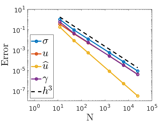
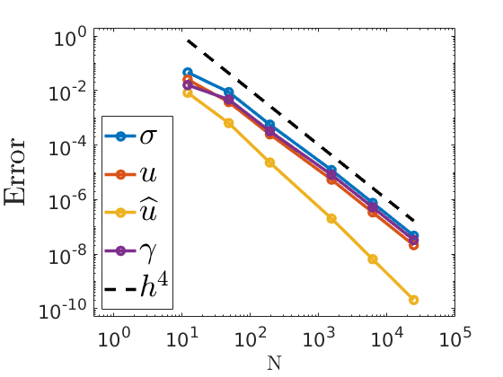
	$\bm{\nu=0.49999}$
Degree $k=1$	Degree $k=2$	Degree $k=3$

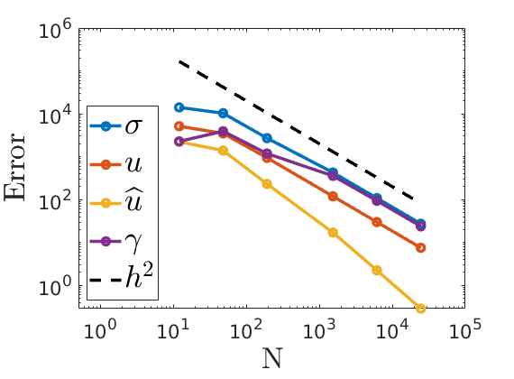
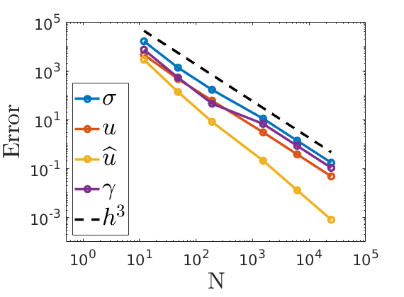
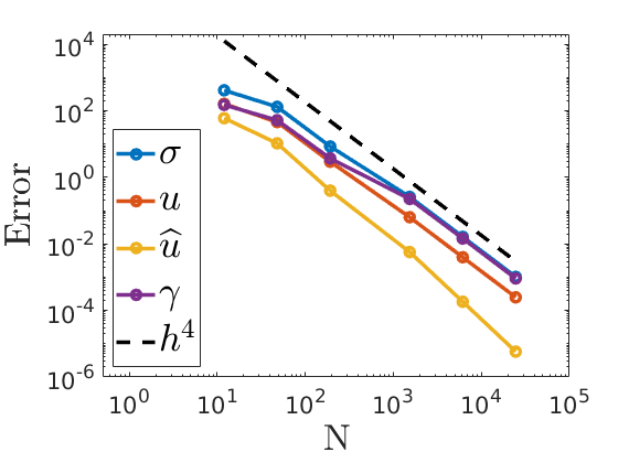
Figure 3: Discretization error as a function of the number of elements in the elastic domain for Poisson’s ratio $\nu=0.3$ (first row) and $\nu=0.49999$ (second row).

The numerical results are shown in Table 2 and Table 3. The same information is plotted in Figure 3. Observe that the experimental orders of convergence of the errors in $\bm{\sigma},\bm{u}$ and $\bm{\gamma}$, $k+1$, coincide with the theoretical results. In addition, for the numerical trace of $\bm{u}$ we also have a superconvergence of order $k+2$.

$\begin{array}[]{c|ccccccccc}\hline\cr\hline\cr\phantom{+}k\phantom{+}&N&\|\bm{\sigma}-\bm{\sigma}_{h}\|_{\mathcal{T}_{E}}&\text{e.o.c.}&\|\bm{u}-\bm{u}_{h}\|_{\mathcal{T}_{E}}&\text{e.o.c.}&{\left|\kern-1.07639pt\left|\kern-1.07639pt\left|\bm{u}-\widehat{\bm{u}}_{h}\right|\kern-1.07639pt\right|\kern-1.07639pt\right|}_{\partial\mathcal{T}_{E}}&\text{e.o.c.}&\|\bm{\gamma}-\bm{\gamma}_{h}\|_{\mathcal{T}_{E}}&\text{e.o.c.}\\ \hline\cr\hbox{\multirowsetup 1}&12&1.10\mathrm{e}{+00}&-&5.71\mathrm{e}{-01}&-&2.98\mathrm{e}{-01}&-&2.92\mathrm{e}{-01}&-\\ &48&6.81\mathrm{e}{-01}&0.70&2.85\mathrm{e}{-01}&1.01&8.67\mathrm{e}{-02}&1.78&3.14\mathrm{e}{-01}&-0.10\\ &192&1.80\mathrm{e}{-01}&1.92&7.77\mathrm{e}{-02}&1.87&1.43\mathrm{e}{-02}&2.60&9.08\mathrm{e}{-02}&1.79\\ &1536&2.08\mathrm{e}{-02}&2.07&1.00\mathrm{e}{-02}&1.97&5.86\mathrm{e}{-04}&3.07&8.78\mathrm{e}{-03}&2.25\\ &6144&5.22\mathrm{e}{-03}&2.00&2.53\mathrm{e}{-03}&1.98&7.54\mathrm{e}{-05}&2.96&2.09\mathrm{e}{-03}&2.07\\ &24576&1.31\mathrm{e}{-03}&2.00&6.36\mathrm{e}{-04}&1.99&9.53\mathrm{e}{-06}&2.98&5.06\mathrm{e}{-04}&2.05\\ \hline\cr\hbox{\multirowsetup 2}&12&9.76\mathrm{e}{-01}&-&3.45\mathrm{e}{-01}&-&1.75\mathrm{e}{-01}&-&5.57\mathrm{e}{-01}&-\\ &48&9.02\mathrm{e}{-02}&3.44&3.79\mathrm{e}{-02}&3.19&8.23\mathrm{e}{-03}&4.41&4.22\mathrm{e}{-02}&3.72\\ &192&1.16\mathrm{e}{-02}&2.96&5.02\mathrm{e}{-03}&2.92&5.25\mathrm{e}{-04}&3.97&5.47\mathrm{e}{-03}&2.95\\ &1536&5.43\mathrm{e}{-04}&2.94&2.57\mathrm{e}{-04}&2.86&8.07\mathrm{e}{-06}&4.02&2.49\mathrm{e}{-04}&2.97\\ &6144&6.80\mathrm{e}{-05}&3.00&3.24\mathrm{e}{-05}&2.99&4.97\mathrm{e}{-07}&4.02&3.12\mathrm{e}{-05}&3.00\\ &24576&8.51\mathrm{e}{-06}&3.00&4.07\mathrm{e}{-06}&2.99&3.09\mathrm{e}{-08}&4.01&3.91\mathrm{e}{-06}&3.00\\ \hline\cr\hbox{\multirowsetup 3}&12&4.64\mathrm{e}{-02}&-&2.53\mathrm{e}{-02}&-&8.33\mathrm{e}{-03}&-&1.59\mathrm{e}{-02}&-\\ &48&8.76\mathrm{e}{-03}&2.41&3.77\mathrm{e}{-03}&2.74&6.40\mathrm{e}{-04}&3.70&4.70\mathrm{e}{-03}&1.76\\ &192&5.63\mathrm{e}{-04}&3.96&2.47\mathrm{e}{-04}&3.94&2.29\mathrm{e}{-05}&4.81&3.23\mathrm{e}{-04}&3.86\\ &1536&1.21\mathrm{e}{-05}&3.70&5.39\mathrm{e}{-06}&3.68&2.02\mathrm{e}{-07}&4.55&8.15\mathrm{e}{-06}&3.54\\ &6144&7.58\mathrm{e}{-07}&3.99&3.39\mathrm{e}{-07}&3.99&6.54\mathrm{e}{-09}&4.95&5.22\mathrm{e}{-07}&3.96\\ &24576&4.74\mathrm{e}{-08}&4.00&2.13\mathrm{e}{-08}&4.00&2.07\mathrm{e}{-10}&4.98&3.29\mathrm{e}{-08}&3.99\\ \hline\cr\hline\cr\end{array}$

Table 2: History of convergence for the elastic variables with $\nu=0.3$ for polynomial basis functions of degree $k$ in a mesh of $N$ elements.

$\begin{array}[]{c|ccccccccc}\hline\cr\hline\cr\phantom{+}k\phantom{+}&N&\|\bm{\sigma}-\bm{\sigma}_{h}\|_{\mathcal{T}_{E}}&\text{e.o.c.}&\|\bm{u}-\bm{u}_{h}\|_{\mathcal{T}_{E}}&\text{e.o.c.}&{\left|\kern-1.07639pt\left|\kern-1.07639pt\left|\bm{u}-\widehat{\bm{u}}_{h}\right|\kern-1.07639pt\right|\kern-1.07639pt\right|}_{\partial\mathcal{T}_{E}}&\text{e.o.c.}&\|\bm{\gamma}-\bm{\gamma}_{h}\|_{\mathcal{T}_{E}}&\text{e.o.c.}\\ \hline\cr\hbox{\multirowsetup 1}&12&1.41\mathrm{e}{+04}&-&5.13\mathrm{e}{+03}&-&2.22\mathrm{e}{+03}&-&2.27\mathrm{e}{+03}&-\\ &48&1.03\mathrm{e}{+04}&0.46&3.48\mathrm{e}{+03}&0.56&1.39\mathrm{e}{+03}&0.67&3.90\mathrm{e}{+03}&-0.78\\ &192&2.70\mathrm{e}{+03}&1.93&9.39\mathrm{e}{+02}&1.89&2.31\mathrm{e}{+02}&2.59&1.18\mathrm{e}{+03}&1.73\\ &1536&4.26\mathrm{e}{+02}&1.78&1.19\mathrm{e}{+02}&1.99&1.70\mathrm{e}{+01}&2.51&3.57\mathrm{e}{+02}&1.15\\ &6144&1.08\mathrm{e}{+02}&1.98&2.99\mathrm{e}{+01}&1.99&2.24\mathrm{e}{+00}&2.92&9.36\mathrm{e}{+01}&1.93\\ &24576&2.73\mathrm{e}{+01}&1.99&7.51\mathrm{e}{+00}&1.99&2.87\mathrm{e}{-01}&2.97&2.38\mathrm{e}{+01}&1.97\\ \hline\cr\hbox{\multirowsetup 2}&12&1.61\mathrm{e}{+04}&-&4.53\mathrm{e}{+03}&-&2.83\mathrm{e}{+03}&-&7.32\mathrm{e}{+03}&-\\ &48&1.34\mathrm{e}{+03}&3.58&4.60\mathrm{e}{+02}&3.30&1.36\mathrm{e}{+02}&4.38&5.25\mathrm{e}{+02}&3.80\\ &192&1.67\mathrm{e}{+02}&3.00&6.03\mathrm{e}{+01}&2.93&8.14\mathrm{e}{+00}&4.06&4.53\mathrm{e}{+01}&3.53\\ &1536&1.10\mathrm{e}{+01}&2.62&3.03\mathrm{e}{+00}&2.88&2.09\mathrm{e}{-01}&3.52&6.70\mathrm{e}{+00}&1.84\\ &6144&1.38\mathrm{e}{+00}&2.99&3.81\mathrm{e}{-01}&2.99&1.29\mathrm{e}{-02}&4.02&8.49\mathrm{e}{-01}&2.98\\ &24576&1.73\mathrm{e}{-01}&3.00&4.77\mathrm{e}{-02}&3.00&8.05\mathrm{e}{-04}&4.00&1.07\mathrm{e}{-01}&2.99\\ \hline\cr\hbox{\multirowsetup 3}&12&4.12\mathrm{e}{+02}&-&1.62\mathrm{e}{+02}&-&5.97\mathrm{e}{+01}&-&1.50\mathrm{e}{+02}&-\\ &48&1.31\mathrm{e}{+02}&1.66&4.54\mathrm{e}{+01}&1.83&1.05\mathrm{e}{+01}&2.51&5.20\mathrm{e}{+01}&1.53\\ &192&8.45\mathrm{e}{+00}&3.95&2.95\mathrm{e}{+00}&3.94&3.98\mathrm{e}{-01}&4.72&3.71\mathrm{e}{+00}&3.81\\ &1536&2.58\mathrm{e}{-01}&3.36&6.32\mathrm{e}{-02}&3.70&5.67\mathrm{e}{-03}&4.09&2.24\mathrm{e}{-01}&2.70\\ &6144&1.63\mathrm{e}{-02}&3.99&3.97\mathrm{e}{-03}&3.99&1.83\mathrm{e}{-04}&4.95&1.45\mathrm{e}{-02}&3.96\\ &24576&1.02\mathrm{e}{-03}&3.99&2.48\mathrm{e}{-04}&4.00&5.79\mathrm{e}{-06}&4.98&9.15\mathrm{e}{-04}&3.98\\ \hline\cr\hline\cr\end{array}$

Table 3: History of convergence for the elastic variables with $\nu=0.49999$ for polynomial basis functions of degree $k$ in a mesh of $N$ elements.

6.3 Coupled problem.

We now test our HDG scheme applied to the coupled problem (1a)-(1h) with Dirichlet boundary conditions $v=g_{D}$ on $\Gamma_{A}$. We take a manufactured acoustic field $v(x,y)=\sin(x)\sin(y)$. The source $f$ and boundary data $g_{D}$ are set in such a way that $v$ satisfies (1c)-(1d) in a domain $\Omega_{A}=(-2,2)^{2}$, with $c=1$ and $s=2-i$. For the elastic region, we consider $\Omega_{E}=(-1,1)^{2},\rho_{E}=1$ and $\tau_{E}=1$ everywhere. The source $\bm{f}$ is defined such that

$$\bm{u}(x,y)=\begin{pmatrix}\sin(\pi x)\cos(\pi y)\\ \cos(\pi x)\sin(\pi y)\end{pmatrix},\quad(x,y)\in(-1,1)^{2},$$

satisfies (1a)-(1b). We set the field $v^{\text{inc}}(x,y)=-\sin(x)\sin(y)$ and include additional terms on the right-hand sides of (1e)-(1f) so that our manufactured solution satisfies them.

In Table 4 and Table 5 we present the numerical results obtained. As in the acoustic and elastic problems, the experimental orders of convergence of $\bm{\sigma}$, $\bm{\gamma}$, $\bm{u}$, $\bm{q}$ and $v$ coincide with the theoretical results. We also computationally obtain the superconvergence of order $k+2$ for the numerical traces. In Figure 4 we graphically show the same results as in the tables.

$\begin{array}[]{c|ccccccccc}\hline\cr\hline\cr\phantom{+}k\phantom{+}&N&\|\bm{\sigma}-\bm{\sigma}_{h}\|_{\mathcal{T}_{E}}&\text{e.o.c.}&\|\bm{u}-\bm{u}_{h}\|_{\mathcal{T}_{E}}&\text{e.o.c.}&{\left|\kern-1.07639pt\left|\kern-1.07639pt\left|\bm{u}-\widehat{\bm{u}}_{h}\right|\kern-1.07639pt\right|\kern-1.07639pt\right|}_{\partial\mathcal{T}_{E}}&\text{e.o.c.}&\|\bm{\gamma}-\bm{\gamma}_{h}\|_{\mathcal{T}_{E}}&\text{e.o.c.}\\[4.30554pt] \hline\cr\hbox{\multirowsetup 1}&80&1.50\mathrm{e}{+00}&-&8.98\mathrm{e}{-01}&-&7.30\mathrm{e}{-01}&-&6.07\mathrm{e}{-01}&-\\ &306&4.84\mathrm{e}{-01}&1.54&2.56\mathrm{e}{-01}&1.71&8.22\mathrm{e}{-02}&2.98&1.99\mathrm{e}{-01}&1.52\\ &1210&1.33\mathrm{e}{-01}&1.92&6.57\mathrm{e}{-02}&2.02&1.04\mathrm{e}{-02}&3.08&6.65\mathrm{e}{-02}&1.63\\ &4824&3.25\mathrm{e}{-02}&2.03&1.62\mathrm{e}{-02}&2.02&1.18\mathrm{e}{-03}&3.13&1.54\mathrm{e}{-02}&2.11\\ &19202&8.26\mathrm{e}{-03}&1.99&4.06\mathrm{e}{-03}&2.00&1.50\mathrm{e}{-04}&2.99&3.87\mathrm{e}{-03}&2.00\\ &76638&2.10\mathrm{e}{-03}&1.97&1.02\mathrm{e}{-03}&1.99&1.93\mathrm{e}{-05}&2.96&9.98\mathrm{e}{-04}&1.96\\ \hline\cr\hbox{\multirowsetup 2}&80&5.13\mathrm{e}{-01}&-&2.48\mathrm{e}{-01}&-&1.11\mathrm{e}{-01}&-&2.31\mathrm{e}{-01}&-\\ &306&6.67\mathrm{e}{-02}&2.78&2.82\mathrm{e}{-02}&2.97&6.73\mathrm{e}{-03}&3.82&3.07\mathrm{e}{-02}&2.75\\ &1210&7.50\mathrm{e}{-03}&3.24&3.77\mathrm{e}{-03}&2.99&3.25\mathrm{e}{-04}&4.50&3.38\mathrm{e}{-03}&3.28\\ &4824&9.28\mathrm{e}{-04}&3.01&4.55\mathrm{e}{-04}&3.05&1.85\mathrm{e}{-05}&4.12&3.85\mathrm{e}{-04}&3.13\\ &19202&1.17\mathrm{e}{-04}&3.00&5.76\mathrm{e}{-05}&3.00&1.13\mathrm{e}{-06}&4.05&4.78\mathrm{e}{-05}&3.03\\ &76638&1.52\mathrm{e}{-05}&2.95&7.28\mathrm{e}{-06}&2.99&7.56\mathrm{e}{-08}&3.91&6.25\mathrm{e}{-06}&2.93\\ \hline\cr\hbox{\multirowsetup 3}&80&6.77\mathrm{e}{-02}&-&3.43\mathrm{e}{-02}&-&1.07\mathrm{e}{-02}&-&3.76\mathrm{e}{-02}&-\\ &306&6.22\mathrm{e}{-03}&3.26&2.78\mathrm{e}{-03}&3.43&4.54\mathrm{e}{-04}&4.31&2.83\mathrm{e}{-03}&3.53\\ &1210&3.75\mathrm{e}{-04}&4.17&1.72\mathrm{e}{-04}&4.13&1.35\mathrm{e}{-05}&5.22&1.87\mathrm{e}{-04}&4.03\\ &4824&2.18\mathrm{e}{-05}&4.10&1.02\mathrm{e}{-05}&4.06&3.57\mathrm{e}{-07}&5.23&9.96\mathrm{e}{-06}&4.23\\ &19202&1.44\mathrm{e}{-06}&3.94&6.59\mathrm{e}{-07}&3.98&1.21\mathrm{e}{-08}&4.90&6.38\mathrm{e}{-07}&3.99\\ &76638&9.50\mathrm{e}{-08}&3.93&4.27\mathrm{e}{-08}&3.95&4.05\mathrm{e}{-10}&4.90&4.15\mathrm{e}{-08}&3.94\\ \hline\cr\hline\cr\end{array}$

Table 4: History of convergence of the coupled problem in the elastic region for polynomial basis functions of degree $k$ in a mesh of $N$ elements.

$\begin{array}[]{c|ccccccc}\hline\cr\hline\cr\phantom{+}k\phantom{+}&N&\|\bm{q}-\bm{q}_{h}\|_{\mathcal{T}_{A}}&\text{e.o.c.}&\|v-v_{h}\|_{\mathcal{T}_{A}}&\text{e.o.c.}&{\left|\kern-1.07639pt\left|\kern-1.07639pt\left|v-\widehat{v}_{h}\right|\kern-1.07639pt\right|\kern-1.07639pt\right|}_{\partial\mathcal{T}_{A}}&\text{e.o.c.}\\[4.30554pt] \hline\cr\hbox{\multirowsetup 1}&80&1.60\mathrm{e}{-01}&-&2.41\mathrm{e}{-02}&-&1.40\mathrm{e}{-01}&-\\ &306&2.10\mathrm{e}{-02}&3.02&4.98\mathrm{e}{-03}&2.35&1.39\mathrm{e}{-02}&3.44\\ &1210&3.69\mathrm{e}{-03}&2.53&9.86\mathrm{e}{-04}&2.36&1.88\mathrm{e}{-03}&2.90\\ &4824&8.40\mathrm{e}{-04}&2.14&2.30\mathrm{e}{-04}&2.10&2.16\mathrm{e}{-04}&3.13\\ &19202&2.05\mathrm{e}{-04}&2.04&6.04\mathrm{e}{-05}&1.94&2.83\mathrm{e}{-05}&2.94\\ &76638&5.17\mathrm{e}{-05}&1.99&1.51\mathrm{e}{-05}&2.00&3.47\mathrm{e}{-06}&3.03\\ \hline\cr\hbox{\multirowsetup 2}&80&3.25\mathrm{e}{-02}&-&6.63\mathrm{e}{-03}&-&2.96\mathrm{e}{-02}&-\\ &306&1.81\mathrm{e}{-03}&4.31&2.32\mathrm{e}{-04}&5.00&7.76\mathrm{e}{-04}&5.43\\ &1210&6.41\mathrm{e}{-05}&4.86&1.19\mathrm{e}{-05}&4.33&2.52\mathrm{e}{-05}&4.99\\ &4824&4.11\mathrm{e}{-06}&3.97&1.88\mathrm{e}{-06}&2.66&5.67\mathrm{e}{-07}&5.49\\ &19202&5.48\mathrm{e}{-07}&2.92&2.54\mathrm{e}{-07}&2.90&1.97\mathrm{e}{-08}&4.86\\ &76638&6.66\mathrm{e}{-08}&3.05&3.00\mathrm{e}{-08}&3.09&8.18\mathrm{e}{-10}&4.60\\ \hline\cr\hbox{\multirowsetup 3}&80&1.82\mathrm{e}{-03}&-&2.45\mathrm{e}{-04}&-&1.36\mathrm{e}{-03}&-\\ &306&1.05\mathrm{e}{-04}&4.26&1.13\mathrm{e}{-05}&4.59&2.35\mathrm{e}{-05}&6.05\\ &1210&2.35\mathrm{e}{-06}&5.53&6.27\mathrm{e}{-07}&4.21&1.96\mathrm{e}{-07}&6.97\\ &4824&4.69\mathrm{e}{-08}&5.66&4.48\mathrm{e}{-08}&3.81&1.61\mathrm{e}{-09}&6.94\\ &19202&2.64\mathrm{e}{-09}&4.17&2.71\mathrm{e}{-09}&4.06&3.55\mathrm{e}{-11}&5.52\\ &76638&1.46\mathrm{e}{-10}&4.18&1.77\mathrm{e}{-10}&3.94&1.77\mathrm{e}{-12}&4.33\\ \hline\cr\hline\cr\end{array}$

Table 5: History of convergence of the coupled problem in the acoustic region for polynomial basis functions of degree $k$ in a mesh of $N$ elements.

	Acoustic variables
Degree $k=1$	Degree $k=2$	Degree $k=3$
​​	​​	​​
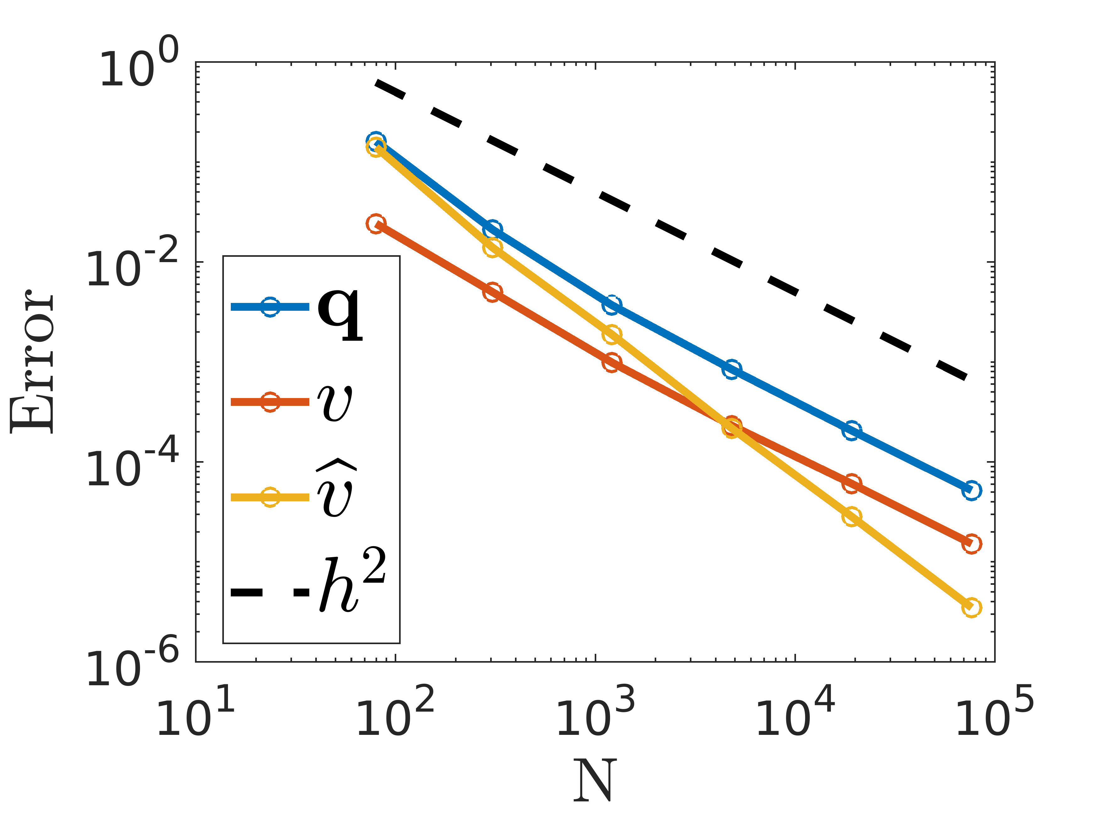
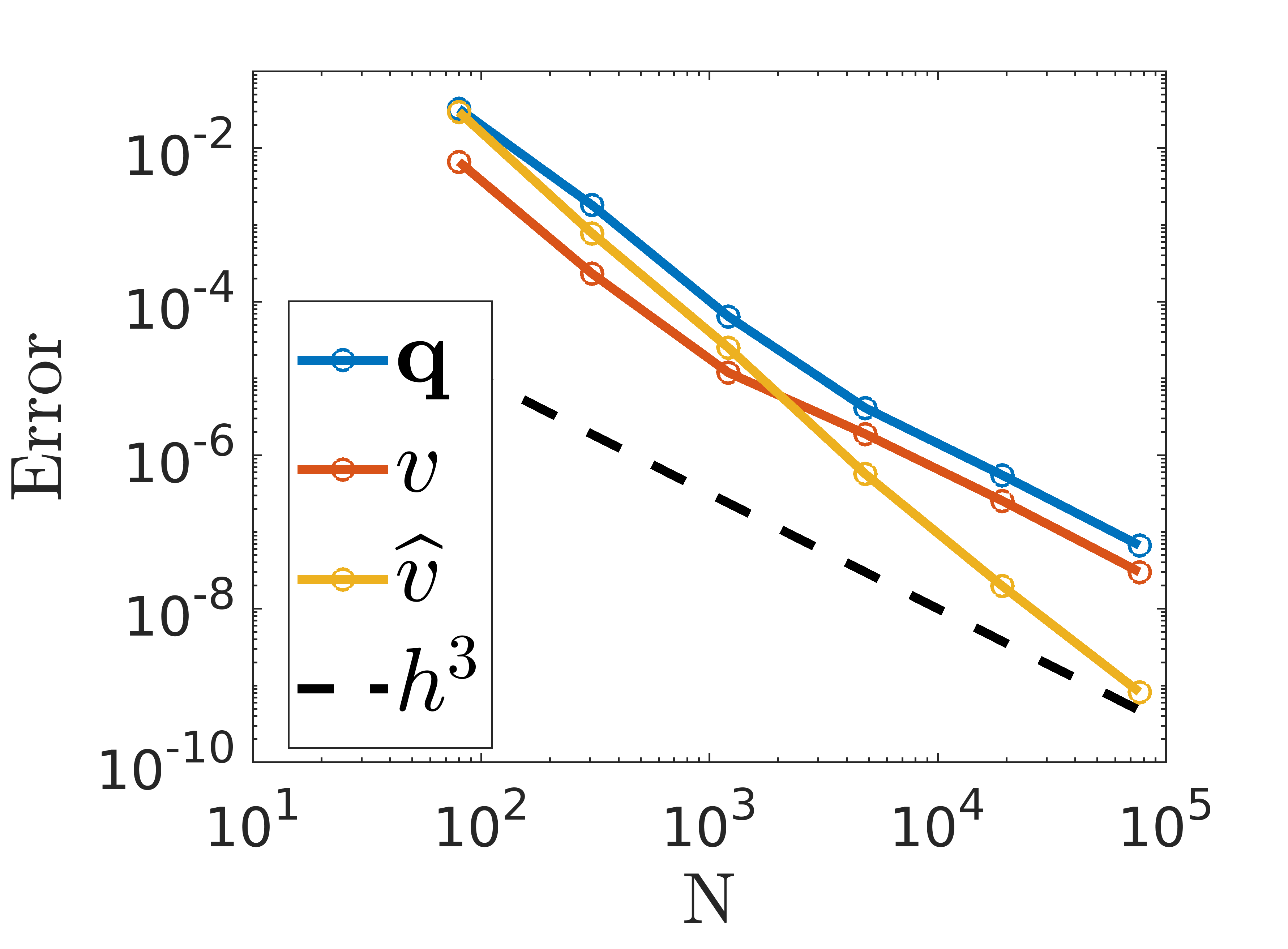
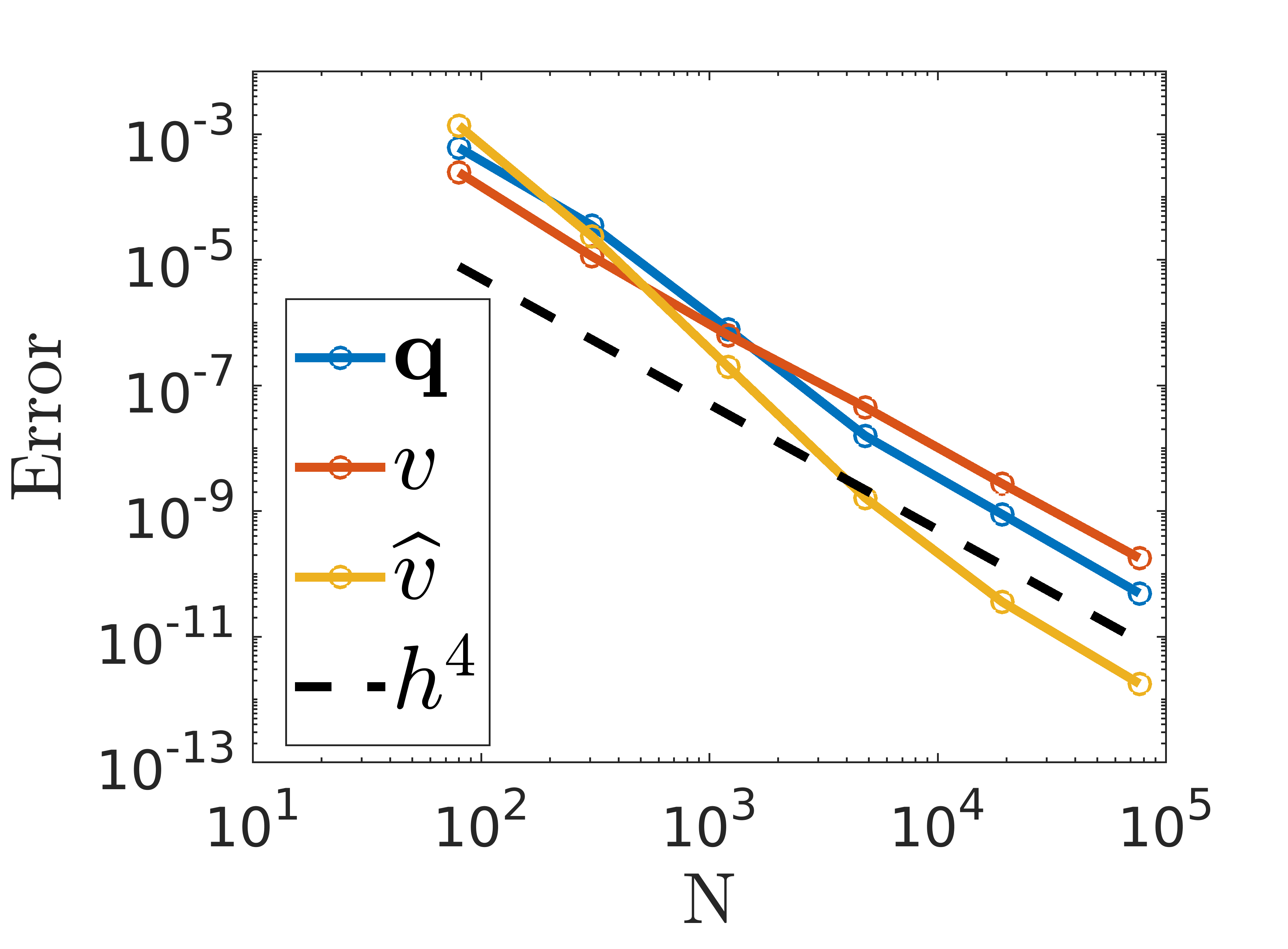
	Elastic Variables
Degree $k=1$	Degree $k=2$	Degree $k=3$
​​	​​	​​

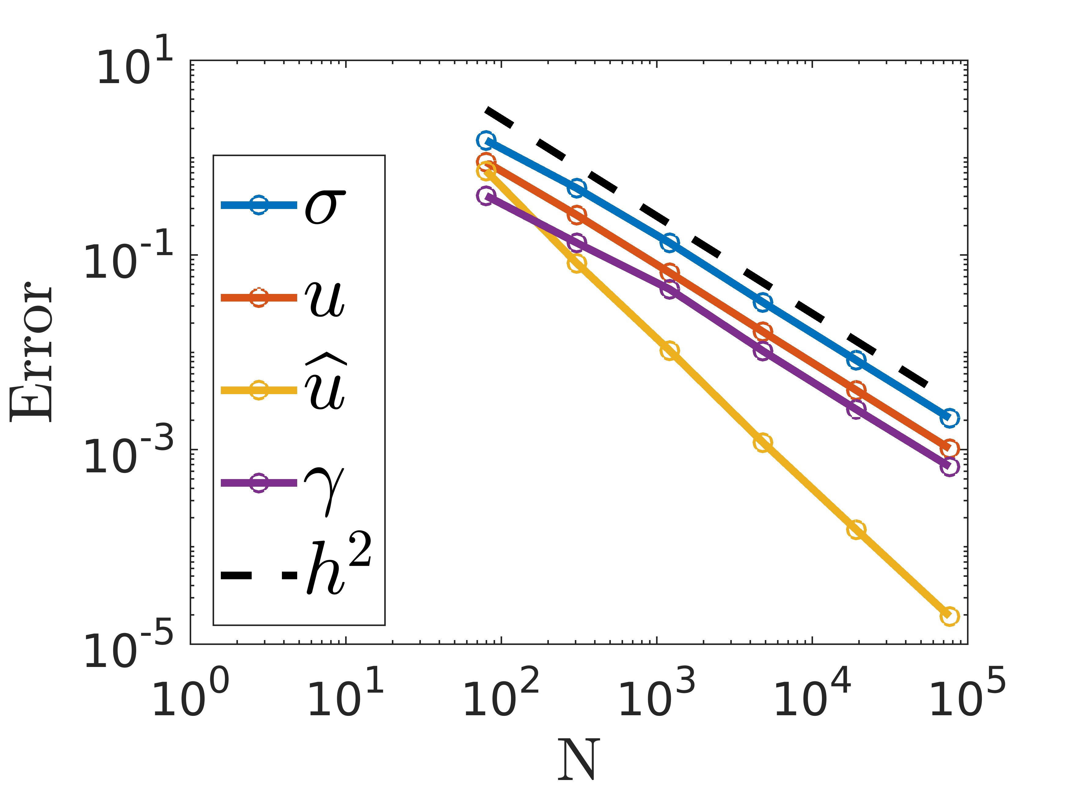
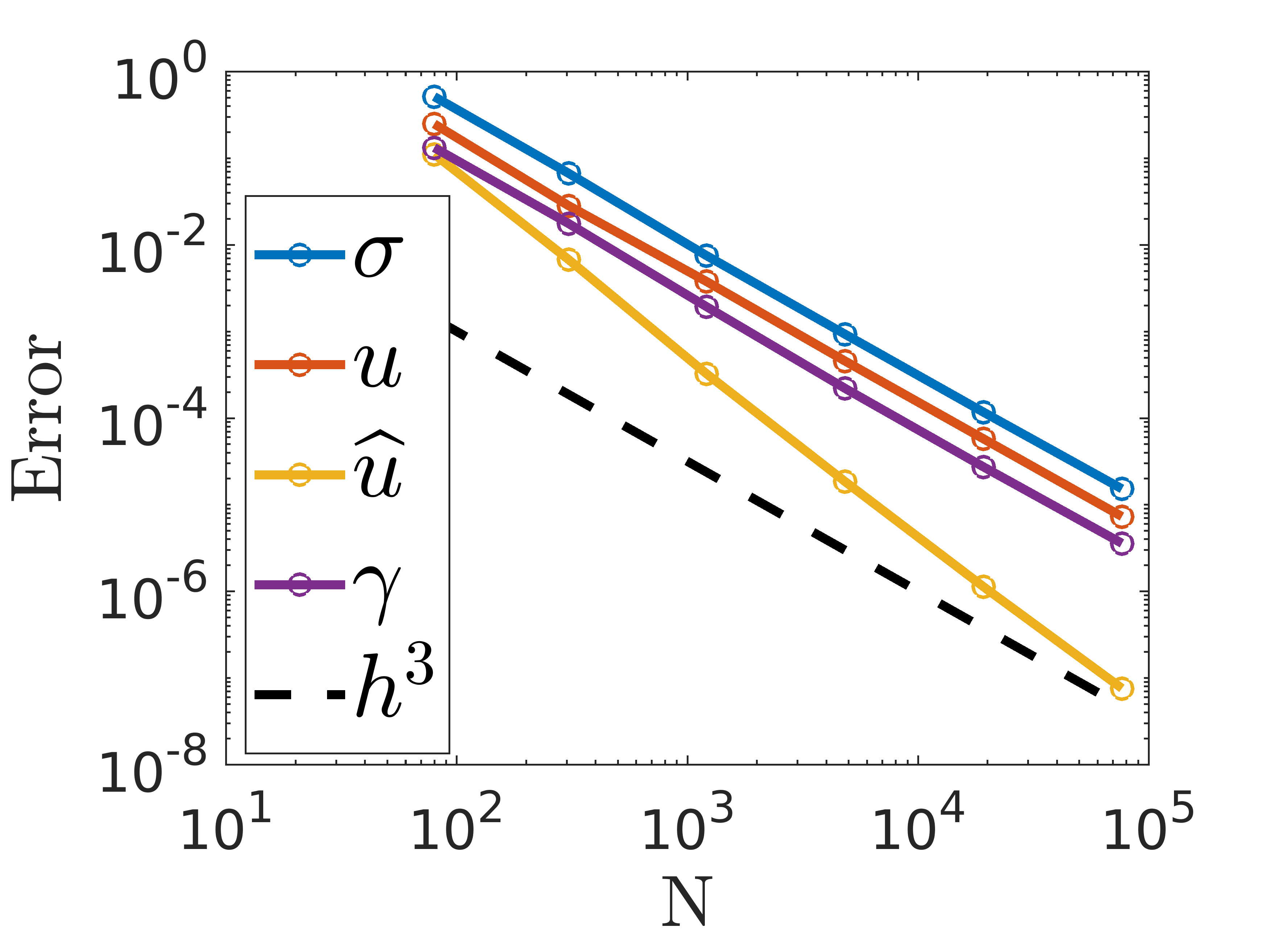
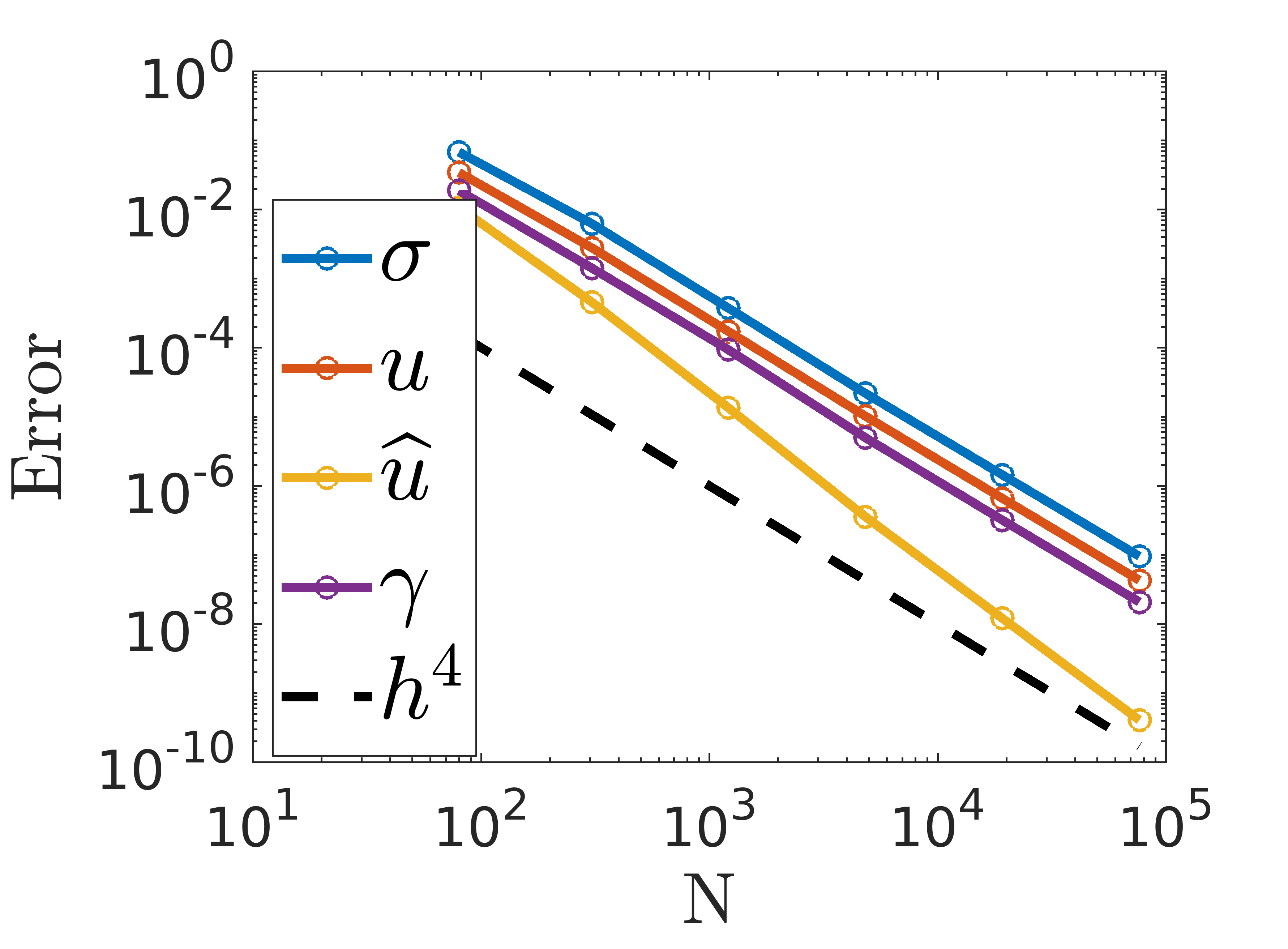
Figure 4: Discretization error as a function of the number of elements in the domain for the coupled acoustic/elastic problem. Acoustic variables are displayed on the first column and elastic variables on the second column.

References

- [1] C. J. S. Alves and P. R. S. Antunes. Wave scattering problems in exterior domains with the method of fundamental solutions. Numerische Mathematik, 156(2):375–394, Feb. 2024.
- [2] R. Araya, R. Rodríguez, and P. Venegas. Numerical analysis of a time domain elastoacoustic problem. IMA Journal of Numerical Analysis, 40(2):1122–1153, 01 2019.
- [3] I. Bermúdez, J. Manríquez, and M. Solano. A hybridizable discontinuous Galerkin method for Stokes/Darcy coupling on dissimilar meshes. IMA J. Numer. Anal., 2025.
- [4] T. S. Brown, T. Sánchez-Vizuet, and F.-J. Sayas. Evolution of a semidiscrete system modeling the scattering of acoustic waves by a piezoelectric solid. ESAIM: Mathematical Modeling and Numerical Analysis (M2AN), 52(2):423–455, 2018. (arXiv:1612.04063).
- [5] R. Bustinza, B. López-Rodríguez, and M. Osorio. An a priori error analysis of an HDG method for an eddy current problem. Mathematical Methods in the Applied Sciences, 41(7):2795–2810, 2018.
- [6] L. Camargo, B. López-Rodríguez, M. Osorio, and M. Solano. An HDG method for Maxwell’s equations in heterogeneous media. Computer Methods in Applied Mechanics and Engineering, 368:113178, 2020.
- [7] J. M. Cárdenas and M. Solano. A high order unfitted hybridizable discontinuous Galerkin method for linear elasticity. IMA Journal of Numerical Analysis, 44(2):945–979, 05 2023.
- [8] A. Cesmelioglu, B. Cockburn, N. C. Nguyen, and J. Peraire. Analysis of HDG methods for Oseen equations. J. Sci. Comput., 55(2):392–431, May 2013.
- [9] A. Cesmelioglu, B. Cockburn, and W. Qiu. Analysis of a hybridizable discontinuous Galerkin method for the steady-state incompressible Navier–Stokes equations. Math. Comp., 86(306):1643–1670, 2017.
- [10] H. Chen, P. Lu, and X. Xu. A hybridizable discontinuous Galerkin method for the Helmholtz equation with high wave number. SIAM Journal on Numerical Analysis, 51(4):2166–2188, 2013.
- [11] H. Chen, W. Qiu, and K. Shi. A priori and computable a posteriori error estimates for an HDG method for the coercive Maxwell equations. Computer Methods in Applied Mechanics and Engineering, 333:287 – 310, 2018.
- [12] H. Chen, W. Qiu, K. Shi, and M. Solano. A superconvergent HDG method for the Maxwell equations. Journal of Scientific Computing, 70(3):1010–1029, 2017.
- [13] Y. Chen and B. Cockburn. Analysis of variable-degree HDG methods for convection-diffusion equations. Part I: general nonconforming meshes. IMA Journal of Numerical Analysis, 32(4):1267–1293, Feb. 2012.
- [14] Y. Chen and B. Cockburn. Analysis of variable-degree HDG methods for convection-diffusion equations. part II: Semimatching nonconforming meshes. Mathematics of Computation, 83(285):87–111, May 2013.
- [15] B. Cockburn, J. Gopalakrishnan, and J. Guzmán. A new elasticity element made for enforcing weak stress symmetry. Mathematics of Computation, 79(271):1331–1349, 2010.
- [16] B. Cockburn, J. Gopalakrishnan, and R. Lazarov. Unified hybridization of discontinuous Galerkin, mixed, and continuous Galerkin methods for second order elliptic problems. SIAM J. Numer. Anal., 47(2):1319–1365, 2009.
- [17] B. Cockburn, J. Gopalakrishnan, N. C. Nguyen, J. Peraire, and F.-J. Sayas. Analysis of HDG methods for Stokes flow. Math. Comp., 80:723–760, 2011.
- [18] B. Cockburn, J. Gopalakrishnan, and F.-J. Sayas. A projection-based error analysis of HDG methods. Mathematics of Computation, 79(271):1351–1367, Mar. 2010.
- [19] B. Cockburn, W. Qiu, and M. Solano. A priori error analysis for HDG methods using extensions from subdomains to achieve boundary conformity. Mathematics of Computation, 83, 03 2014.
- [20] B. Cockburn and K. Shi. Superconvergent HDG methods for linear elasticity with weakly symmetric stresses. IMA Journal of Numerical Analysis, 33(3):747–770, 10 2012.
- [21] B. Cockburn and M. Solano. Solving Dirichlet boundary-value problems on curved domains by extensions from subdomains. SIAM Journal on Scientific Computing, 34(1):A497–A519, 2012.
- [22] C. Domínguez, G. N. Gatica, and S. Meddahi. A posteriori error analysis of a fully-mixed finite element method for a two-dimensional fluid-solid interaction problem. Journal of Computational Mathematics, 33(6):606–641, 2015.
- [23] B. Engquist and A. Majda. Absorbing boundary conditions for the numerical simulation of waves. Mathematics of Computation, 31(139):629–651, 1977.
- [24] X. Feng, P. Lu, and X. Xu. A hybridizable discontinuous Galerkin method for the time-harmonic Maxwell equations with high wave number. Computational Methods in Applied Mathematics, 16(3):429–445, 2016.
- [25] G. Fu, Y. Jin, and W. Qiu. Parameter-free superconvergent -conforming HDG methods for the Brinkman equations. arXiv:1607.07662 [math.NA], July 2016.
- [26] G. Fu, W. Qiu, and W. Zhang. An analysis of HDG methods for convection–dominated diffusion problems. ESAIM: M2AN, 49(1):225–256, 2015.
- [27] G. N. Gatica, N. Heuer, and S. Meddahi. Coupling of mixed finite element and stabilized boundary element methods for a fluid–solid interaction problem in 3d. Numerical Methods for Partial Differential Equations, 30(4):1211–1233, 2014.
- [28] G. N. Gatica, A. Márquez, and S. Meddahi. Analysis of the coupling of Lagrange and Arnold-Falk-Winther finite elements for a fluid-solid interaction problem in three dimensions. SIAM Journal on Numerical Analysis, 50(3):1648–1674, 2012.
- [29] G. N. Gatica and F. A. Sequeira. A priori and a posteriori error analyses of an augmented HDG method for a class of quasi-Newtonian Stokes flows. J. Sci. Comput., 69:1192–1250, 2016.
- [30] G. N. Gatica and F. A. Sequeira. Analysis of the HDG method for the Stokes–Darcy coupling. Numer. Methods Partial Differential Equations, 33(3):885–917, 2017.
- [31] R. Griesmaier and P. Monk. Error analysis for a hybridizable discontinuous Galerkin method for the Helmholtz equation. Journal of Scientific Computing, 49(3):291–310, 2011.
- [32] J. Guzmán. A unified analysis of several mixed methods for elasticity with weak stress symmetry. Journal of Scientific Computing, 44:156–169, 2010.
- [33] L. Halpern and L. N. Trefethen. Wide‐angle one‐way wave equations. The Journal of the Acoustical Society of America, 84(4):1397–1404, 10 1988.
- [34] R. L. Higdon. Numerical absorbing boundary conditions for the wave equation. Mathematics of Computation, 49(179):65–90, 1987.
- [35] G. C. Hsiao and T. Sánchez-Vizuet. Time-dependent wave-structure interaction revisited: Thermo-piezoelectric scatterers. Fluids, 6(3), 2021. (arXiv: 2102.04118).
- [36] G. C. Hsiao, T. Sánchez-Vizuet, and F.-J. Sayas. Boundary and coupled boundary-finite element methods for transient wave-structure interaction. IMA Journal of Numerical Analysis, 37(1):237–265, 2016. (arXiv:1509.01713).
- [37] L. N. T. Huynh, N. C. Nguyen, J. Peraire, and B. C. Khoo. A high-order hybridizable discontinuous Galerkin method for elliptic interface problems. International Journal for Numerical Methods in Engineering, 93(2):183–200, jan 2013.
- [38] Q.-H. Liu and J. Tao. The perfectly matched layer for acoustic waves in absorptive media. The Journal of the Acoustical Society of America, 102(4):2072–2082, 10 1997.
- [39] J. Manríquez, N.-C. Nguyen, and M. Solano. A dissimilar non-matching HDG discretization for Stokes flows. Comput. Methods Appl. Mech. Engrg., 399:Paper No. 115292, 30, 2022.
- [40] S. Meddahi, D. Mora, and R. Rodríguez. Finite element analysis for a pressure–stress formulation of a fluid–structure interaction spectral problem. Computers & Mathematics with Applications, 68(12, Part A):1733–1750, 2014.
- [41] N. C. Nguyen, J. Peraire, and B. Cockburn. An implicit high–order hybridizable discontinuous Galerkin method for linear convection–diffusion equations. J. Comput. Phys., 228(9):3232–3254, 2009.
- [42] N. C. Nguyen, J. Peraire, and B. Cockburn. Hybridizable discontinuous Galerkin methods for the time-harmonic Maxwell’s equations. Journal of Computational Physics, 230(19):7151–7175, 2011.
- [43] N. C. Nguyen, J. Peraire, and B. Cockburn. An implicit high-order hybridizable discontinuous Galerkin method for the incompressible Navier–Stokes equations. J. Comput. Phys., 230(4):1147–1170, 2011.
- [44] W. Qiu, J. Shen, and K. Shi. HDG method for linear elasticity with strong symmetric stresses. Mathematics of Computations, 87:69–93, 2018.
- [45] N. Sánchez, T. Sánchez-Vizuet, and M. Solano. Error analysis of an unfitted HDG method for a class of non-linear elliptic problems. Journal of Scientific Computing, 90(3), Feb. 2022. (arXiv: 2105.03560).
- [46] N. Sánchez, T. Sánchez-Vizuet, and M. E. Solano. A priori and a posteriori error analysis of an unfitted HDG method for semi-linear elliptic problems. Numerische Mathematik, 148(4):919–958, Aug. 2021. (arXiv:1911.12298).
- [47] N. Sánchez, T. Sánchez-Vizuet, and M. E. Solano. Afternote to “Coupling at a Distance”: Convergence analysis and a priori error estimates. Computational Methods in Applied Mathematics, 22(4):945–970, 2022.
- [48] T. Sánchez-Vizuet. Integral and coupled integral-volume methods for transient problems in wave-structure interaction. Phd thesis, University of Delaware, Newark, DE, 2016. Available at https://udspace.udel.edu/items/88d8c2c7-633a-456c-90b7-4a7a60ca7317.
- [49] T. Sánchez-Vizuet. A symmetric boundary integral formulation for time-domain acoustic-elastic scattering. (Submitted), 2025. arXiv:2502.04767.
- [50] T. Sánchez-Vizuet and M. E. Solano. A Hybridizable Discontinuous Galerkin solver for the Grad-Shafranov equation. Computer Physics Communications, 235:120 – 132, 2019. (arXiv:1712.04148).
- [51] T. Sánchez-Vizuet, M. E. Solano, and A. J. Cerfon. Adaptive hybridizable discontinuous Galerkin discretization of the Grad-Shafranov equation by extension from polygonal subdomains. Computer Physics Communications, 255:107239, 2020. (arXiv:1903.01724).
- [52] M. Solano, S. Terrana, N.-C. Nguyen, and J. Peraire. An HDG method for dissimilar meshes. IMA J. Numer. Anal., 42(2):1665–1699, 2022.
- [53] L. N. Trefethen and L. Halpern. Well-posedness of one-way wave equations and absorbing boundary conditions. Mathematics of Computation, 47(176):421–435, 1986.
- [54] B. Wang and B. C. Khoo. Hybridizable discontinuous Galerkin method (HDG) for Stokes interface flow. Journal of Computational Physics, 247:262–278, Aug. 2013.
- [55] B. Zhu and H. Wu. Preasymptotic error analysis of the HDG method for Helmholtz equation with large wave number. Journal of Scientific Computing, 87(2):1–34, 2021.