Khan-GCL: Kolmogorov–Arnold Network Based Graph Contrastive Learning with Hard Negatives

Abstract

Graph contrastive learning (GCL) has demonstrated great promise for learning generalizable graph representations from unlabeled data. However, conventional GCL approaches face two critical limitations: (1) the restricted expressive capacity of multilayer perceptron (MLP) based encoders, and (2) suboptimal negative samples that either from random augmentations—failing to provide effective ‘hard negatives’—or generated hard negatives without addressing the semantic distinctions crucial for discriminating graph data. To this end, we propose Khan-GCL, a novel framework that integrates the Kolmogorov–Arnold Network (KAN) into the GCL encoder architecture, substantially enhancing its representational capacity. Furthermore, we exploit the rich information embedded within KAN coefficient parameters to develop two novel critical feature identification techniques that enable the generation of semantically meaningful hard negative samples for each graph representation. These strategically constructed hard negatives guide the encoder to learn more discriminative features by emphasizing critical semantic differences between graphs. Extensive experiments demonstrate that our approach achieves state-of-the-art performance compared to existing GCL methods across a variety of datasets and tasks.

1 Introduction

Graph Neural Networks (GNNs) are a class of machine learning models designed to learn from graph-structured data and are critical for tasks such as social network analysis, molecular property prediction, and recommendation systems. Integrating self-supervised contrastive learning (CL) that has gained popularity across a variety of domains Oord et al. (2018); Chen et al. (2020); Gao et al. (2021); Radford et al. (2021) into graph learning has given rise to Graph Contrastive Learning (GCL), enabling pre-training GNN encoders from unlabeled graph data Veličković et al. (2018); You et al. (2020); Zhu et al. (2020); You et al. (2021).

However, how to train good GCL models for real-world applications where labeled nodes or graphs are scarce or unavailable is confronted with two challenges. First, existing GCL models employ Multilayer Perceptron (MLP)-based encoders while facing a dilemma: shallow MLPs limit the generalization ability of the encoder Zhang et al. (2024a) while deep MLPs can easily overfit Chen et al. (2022); Rong et al. (2019). In addition, deep GNN encoders can overcompress, distort, or homogenize node features, and hence exacerbate the inherent over-smoothing in GNNs, making node representations indistinguishable from each other and leading to performance degradations Li et al. (2018). These difficulties have rendered use of MLP encoders with a limited depth. But in general, while being critical, striking a good balance between expressiveness and need for mitigating deep GNNs’ inherent problems is difficult.

Second, the performance of GCL heavily relies on the construction of augmented graph data pairs. Positive pairs consist of distinct views derived from the same graph using random, handcrafted, or saliency-guided augmentations You et al. (2020, 2021); Zhang et al. (2024c); Li et al. (2022); Wei et al. (2023), which help the encoder learn semantically similar graph features. Conversely, negative pairs, comprising views from different graphs, provide crucial information about semantic differences and thus encourage the learning of discriminative features You et al. (2020, 2021); Xia et al. (2021); Zhang et al. (2024b). In CL literature, hard negatives refer to samples from different classes that share similar latent semantic features with a target data point. Recent studies Kalantidis et al. (2020); Xia et al. (2021); Luo et al. (2023); Wang et al. (2024) demonstrate that incorporating such hard negatives significantly improves the encoder’s performance on downstream tasks by making contrastive loss minimization more challenging. However, generating high-quality hard negatives remains a non-trivial task. The methods in Chen et al. (2020); He et al. (2020); Cui et al. (2021) enlarge the training batch size to include more negatives, but without guaranteeing inclusion of more hard negatives, this can lead to performance degradationChen et al. (2020); Kalantidis et al. (2020); He et al. (2020). Additionally, the absence of labels in unsupervised pre-training renders the introduction of ‘false negatives’, formed by pairs of samples belonging to the same class Kalantidis et al. (2020); Xia et al. (2021). Adversarial approaches generate negatives without explicitly identifying which latent features are most crucial to discriminate negative pairs Hu et al. (2021); Luo et al. (2023); Zhang et al. (2024b); Wang et al. (2024). Therefore, more effective methods are desired for generating hard negative pairs to improve the performance of GCL.

We believe that tackling the challenges brought by lack or scarcity of labeled graph data and the resulting overfitting and other inherent GNN problems in real-world applications requires advances in both GCL model architecture and data augmentation, the latter of which is at the core of graph-based contrastive learning. To this end, we propose Khan-GCL: KAN-based hard negative generation for GCL. In terms of model architecture, we replace typical MLP encoders with Kolmogorov-Arnold Network (KAN) Liu et al. (2024). By integrating the Kolmogorov-Arnold representation theorem into modern neural networks, KAN introduces parameterized and learnable non-linear activation functions on the edges (i.e., weights) of the network, replacing traditional fixed activation functions in MLPs Hornik et al. (1989); Cybenko (1989). KANs impose a localized structure on the trainable functions through their spline-based kernel activations. This acts as a form of regularization, guiding the model to learn smoother mappings that generalize better. In contrast, standard neural networks with fixed nonlinearities are more prone to overfitting when training data is limited. This increases representational power without requiring a deeper network, which is critical for avoiding overfitting when data is scarce. As a result, KAN-based encoders strike a better balance between expensiveness and risks of inherent issues in deep GNNs.

In terms of data augmentation, we develop a method, called Critical KAN Feature Identification (CKFI), for generating hard negatives in the output representation space of each KAN encoder to better train them through contrastive learning. By exploiting the global nature of the B-spline coefficients describing KAN encoders’ output features, CKFI identifies two types of critical features—discriminative and independent features—that highlight the most sensitive and distinctive dimensions of the underlying graph structure. Perturbing these critical features alters the essential semantics of the graph and hence generates negative pairs, which can be made hard with a small perturbation magnitude. The generated high-quality hard negatives improve the encoder’s ability to discriminate subtle but crucial semantics in downstream tasks.

Our main contributions of this paper include:

1. We propose Khan-GCL, the first graph contrastive learning framework that integrates Kolmogorov-Arnold Network (KAN) encoders into contrastive learning, increasing the expressive power of GNNs.

2. We introduce CKFI, a novel approach for identifying two types of critical KAN output features, which are most independent and most discriminative of varying underlying graph structures, by exploiting the global nature of the learned B-spline coefficients from KAN encoders.

3. We present a new method that minimally perturbs the most critical output features of each KAN encoder to generate semantically meaningful hard negatives, thereby enhancing the effectiveness of graph contrastive learning.

Experiments across various biochemical and social media datasets demonstrate that our method achieves state-of-the-art performance on different tasks.

Figure 1: Overview of the Khan-GCL framework. The encoder utilizes KAN to enhance expressive power and interpretability. Leveraging the KAN architecture, we introduce two critical dimension identification techniques. By applying small perturbations to these identified dimensions, we generate hard negative samples for each graph, thereby improving the performance of this GCL approach.

2 Related works

2.1 Graph Contrastive Learning (GCL)

Graph Contrastive Learning (GCL) is capable of learning powerful representations from unlabeled graph data Veličković et al. (2018); You et al. (2020); Zhu et al. (2020); You et al. (2021). Typically, GCL employs random data augmentation strategies to generate diverse views of each graph, forming positive pairs from augmented views of the same graph and negative pairs from different graphs You et al. (2020). Subsequent research has introduced automated You et al. (2021), domain-knowledge informed Zhu et al. (2021); Wang et al. (2021), and saliency-guided Li et al. (2025); Liu et al. (2021); Li et al. (2022) augmentation approaches to further improve representation quality.

Recent studies in CL Kalantidis et al. (2020); Xia et al. (2021) emphasize the significance of hard negatives, demonstrating their effectiveness in enhancing downstream task performance. While prior research Chen et al. (2020); Cui et al. (2021) suggests that enlarging training batch size to include more negative samples can improve feature discrimination, merely increasing the number of negatives does not inherently yield harder negative samples. In fact, continually increasing batch size can lead to performance degradation in contrastive learning Chen et al. (2020); Kalantidis et al. (2020); He et al. (2020). To explicitly introduce hard negatives, Kalantidis et al. (2020); Xia et al. (2021) propose ranking existing negatives in a mini-batch based on their similarity and mixing the hardest examples to produce hard negatives. However, the absence of labels in unsupervised pre-training may introduce ‘false negatives’, negative pairs formed by samples belonging to the same class. More recent approaches frame hard negative generation in GCL as an adversarial process Hu et al. (2021); Luo et al. (2023); Zhang et al. (2024b); Wang et al. (2024), wherein a negative generator attempts to maximize the contrastive loss while the encoder aims to minimize it. However, current adversarial approaches primarily focus on bringing negative pairs closer without explicitly identifying critical latent dimensions responsible for semantic differences.

2.2 Kolmogorov-Arnold Networks in Graph Learning

Kolmogorov-Arnold Network (KAN) Liu et al. (2024) is a novel neural network architecture demonstrating improved generalization ability and interpretability over MLPs. Many recent studies Kiamari et al. (2024); Zhang and Zhang (2024); Bresson et al. (2025); Li et al. (2024b) have proposed KAN-based GNN architectures by directly replacing MLPs in conventional models like GCN/GIN with KAN. These investigations reveal that KAN effectively enhances the generalization capacity of traditional GNNs while mitigating the over-squashing problem inherent in MLP-based architectures. Furthermore, several studies have demonstrated KAN’s superior generalizability over MLPs in specialized domains, including drug discovery Ahmed and Sifat (2024), molecular property prediction Li et al. (2024a), recommendation systems Xu et al. (2024), and smart grid intrusion detection Wu et al. (2025).

Beyond straightforward MLP substitution, KAA Fang et al. (2025) embeds KANs into the attention scoring functions of GAT and Transformer-based models. KA-GAT Chen et al. (2025) combines KAN-based feature decomposition with multi-head attention and graph convolutions, enhancing the model’s capacity in high-dimensional graph data.

3 Preliminary

Graph Contrastive Learning

aims to train an encoder $f(\cdot):\mathbb{R}^{m}\to\mathbb{R}^{n}$ which maps graph data $\mathbf{x}\in\mathbb{R}^{m}$ to representations $\mathbf{z}\in\mathbb{R}^{n}$. In pre-training, a projection head $h(\cdot):\mathbb{R}^{n}\to\mathbb{R}^{p}$ is often employed to project the representations to $v\in\mathbb{R}^{p}$. GCL typically applies two random augmentation functions $A_{1}(\cdot)$ and $A_{2}(\cdot)$, sampled from a set $\mathcal{A}$ of augmentations, to produce two views of each graph from a batch $\mathcal{B}_{o}=\{\mathbf{x}_{i}^{o}\}_{i=1}^{N}$ and get a batch of augmented graphs $\mathcal{B}=\{\mathbf{x}_{i}\}_{i=1}^{2N}$, where $\mathbf{x}_{2i}=A_{1}(\mathbf{x}_{i}^{0})$, $\mathbf{x}_{2i+1}=A_{2}(\mathbf{x}_{i}^{0})$. These views are then encoded and projected to $\mathbb{R}^{p}$, i.e., $\mathbf{z}_{i}=f(\mathbf{x}_{i})$ and $\mathbf{v}_{i}=h(\mathbf{z}_{i})$. A contrastive loss Oord et al. (2018); Chen et al. (2020); You et al. (2020) is applied to encourage similarity between positive pairs and dissimilarity between negative pairs:

$$\mathcal{L}_{CL}=\frac{1}{2N}\sum_{i=1}^{N}{-}[\mathrm{log}\frac{\mathrm{exp}(\mathrm{sim}(\mathbf{v}_{2i},\mathbf{v}_{2i+1})/\tau)}{\sum_{j\neq 2i}\mathrm{exp}(\mathrm{sim}(\mathbf{v}_{2i},\mathbf{v}_{j})/\tau)}{+}\mathrm{log}\frac{\mathrm{exp}(\mathrm{sim}(\mathbf{v}_{2i+1},\mathbf{v}_{2i})/\tau)}{\sum_{j\neq 2i+1}\mathrm{exp}(\mathrm{sim}(\mathbf{v}_{2i+1},\mathbf{v}_{j})/\tau)}]$$ (1)

Here $\mathrm{sim}(\cdot,\cdot)$ calculates the cosine similarity between two vectors. $\tau$ is a temperature hyperparameter. Although various GCL methods have been developed, their contrastive loss are defined similarly.

Kolmogorov-Arnold Networks

integrate the Kolmogorov–Arnold representation theorem into modern neural networks. A KAN layer $\mathbf{\Phi}$, which maps input data from $\mathbb{R}^{d_{in}}$ to $\mathbb{R}^{d_{out}}$, is defined as:

$$x_{j}^{out}=\sum_{i=1}^{d_{in}}\phi_{i,j}(x_{i}^{in})\qquad\forall j\in\{1,2,\dots,d_{out}\}$$ (2)

$x_{i}^{in}$ and $x_{j}^{out}$ denote the input and output components at dimensions $i$ and $j$, respectively. Each univariate function $\phi_{i,j}$ represents a learnable non-linear function associated with the connection from the $i_{th}$ input dimension to the $j_{th}$ output dimension. These functions are usually parameterized using B-splines Liu et al. (2024), such that:

$$\phi_{i,j}(\cdot)=\sum_{k}c_{ijk}B_{ijk}(\cdot)$$ (3)

$B_{ijk}(\cdot)$ denotes the B-spline basis functions for $\phi_{i,j}(\cdot)$, and $c_{ijk}$ represents their corresponding trainable coefficients. All coefficients at a KAN layer can thus be denoted as $\mathbfcal{C}=\{c_{ijk}\}\in\mathbb{R}^{d_{in}\times d_{out}\times d_{c}}$, where $d_{c}$ is the number of coefficients used to define each B-spline function.

4 Method

4.1 Overview

Figure 1 illustrates Khan-GCL, the first GCL framework with a KAN-based encoder. By parameterizing non-linearity with trainable basis function coefficients, KANs offer improved generalizability and interpretability over conventional MLPs. Leveraging the rich non-linear information in KAN coefficients, we introduce CKFI (Section 4.2) to identify two types of critical features. Small perturbations applied to these features generate hard negatives that alter sample semantics while preserving structural similarity (Section 4.3). Incorporating these hard negatives during pre-training guides the encoder to learn more discriminative graph features.

4.2 Critical KAN Feature Identification (CKFI)

4.2.1 Independent Dimensions in KANs

According to Equation 2, each latent dimension in a KAN layer combines a unique set of non-linear functions, capturing distinct non-linear features from the input. However, as each B-spline function is a linear combination of basis functions $B_{ijk}(\cdot)$ (Equation 3), an output dimension whose coefficients are linearly dependent on those of other dimensions can be represented as a linear combination of them, making it contain redundant information. Conversely, we define an independent dimension as one whose coefficients cannot be expressed as linear combinations of coefficients from other dimensions, thus encoding truly unique features globally from the entire input domain.

To identify independent dimensions in a KAN layer, as illustrated in Figure 2(a), we attempt to reconstruct the original coefficient tensor $\mathbfcal{C}$ of the layer after removing coefficients from each output dimension. Specifically, given the coefficients $\mathbfcal{C}=[c_{ijk}]\in\mathbb{R}^{d_{in}\times d_{out}\times d_{c}}$ from a KAN layer, we perform higher-order singular value decomposition (HOSVD) with each output dimension $d_{j},1\leq j\leq d_{out}$ removed as follows:

$$\mathbfcal{C}^{(-j)}\approx\mathbfcal{G}\times_{1}\mathbf{U}^{(1)}\times_{2}\mathbf{U}^{(2)}\times_{3}\mathbf{U}^{(3)}$$ (4)

Here $\mathbfcal{C}^{(-j)}\in\mathbb{R}^{d_{in}\times(d_{out}-1)\times d_{c}}$ denotes the tensor obtained by removing the $j_{th}$ mode-$2$ slice from $\mathbfcal{C}$. $\mathbfcal{G}\in\mathbb{R}^{r_{1}\times r_{2}\times r_{3}}$ is the core tensor containing singular values of $\mathbfcal{C}^{(-j)}$, and $\mathbf{U}^{(1)},\mathbf{U}^{(2)},\mathbf{U}^{(3)}$ are orthogonal bases for each mode of $\mathbfcal{C}^{(-j)}$. The notation $\times_{n}$ denotes the mode-$n$ tensor product. A detailed implementation of HOSVD is provided in Appendix B.

Then we reconstruct the coefficients $\mathbfcal{C}$ using $\mathbfcal{C}^{(-j)}$. First, we project the removed $j_{th}$ mode-$2$ slice back to the subspace spanned by $\mathbf{U}^{(1)}$ and $\mathbf{U}^{(3)}$ to get $\tilde{\mathbf{M}}_{j}^{(2)}$. Integrating $\tilde{\mathbf{M}}_{j}^{(2)}$ into $\mathbf{U}^{(2)}\in\mathbb{R}^{r_{2}\times(d_{out}-1)}$, we get $\tilde{\mathbf{U}}_{j}^{(2)}\in\mathbb{R}^{r_{2}\times d_{out}}$, the approximated basis $\mathbf{U}_{j}^{(2)}$ including the $j_{th}$ dimension. Subsequently, we reconstruct $\mathbfcal{C}$ as follows:

$$\tilde{\mathbfcal{C}}_{j}=\mathbfcal{G}\times_{1}\mathbf{U}^{(1)}\times_{2}\tilde{\mathbf{U}}_{j}^{(2)}\times_{3}\mathbf{U}^{(3)}$$ (5)

where $\tilde{\mathbfcal{C}}_{j}$ is the reconstruction with the $j_{th}$ mode-$2$ slice removed from $\mathbfcal{C}$. The reconstruction error can be calculated using the Frobenius norm:

$$\delta_{j}=\|\tilde{\mathbfcal{C}}_{j}-\mathbfcal{C}\|_{F}$$ (6)

A larger reconstruction error $\delta_{j}$ indicates that the $j_{th}$ output dimension encodes more unique features, as it becomes difficult to be accurately reconstructed when excluded from the tensor decomposition. For clarity, the algorithm for identifying independent features is provided in Appendix C.

4.2.2 Discriminative Dimensions in KANs

In this section, we focus on discriminative dimensions, which provides an orthogonal perspective to the aforementioned independent dimension identification technique. In discrimination tasks, latent dimensions exhibiting larger output variance are preferred since they effectively separate different data points. Such dimensions are considered critical as they play a pivotal role in downstream classification tasks.

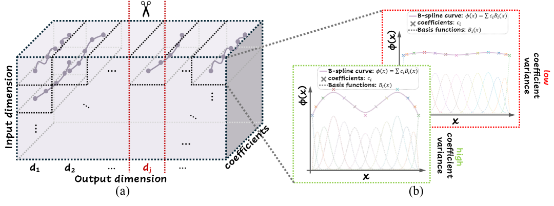
Figure 2: Illustration of a KAN layer and our two proposed critical feature identification techniques. (a) An output dimension is deemed independent when its removal from the coefficient tensor prevents accurate reconstruction of the original tensor (i.e., results in great reconstruction error). (b) Output dimensions comprising B-splines with high coefficient variance are considered discriminative, as larger coefficient variance typically corresponds to greater functional variance.

To implement discriminative feature identification in practice, one can naively sample mini-batches from a dataset and calculate the variance at each dimension. However, estimating variance from randomly sampled mini-batches can introduce bias and additional computational overhead. Instead, we examine the coefficients of KAN layers, which provide a ‘global’ view of the distribution of the underlying features. As illustrated in Figure 2(b), the shape of a B-spline curve closely aligns with the pattern of its coefficients. To formally establish this observation, we present the following proposition, establishing an upper bound on the variance of a uniform B-spline function based on its coefficients’ variance.

Proposition 1 (Variance Upper Bound of a Uniform B-spline Function)

$\phi(x)=\sum_{k}c_{k}B_{k}(x)$ is a uniform B-spline function defined over the interval $[a,b]$. $\{B_{k}(x)\}_{k=1}^{d_{c}}$ denotes the set of uniform B-spline basis functions and $\{c_{k}\}_{k=1}^{d_{c}}$ are the corresponding coefficients. The variance of $\phi(x)$ of its input domain satisfies the following inequality:

$$\mathrm{Var}[\phi(x)]=\int_{a}^{b}(\phi(x)-\mu_{\phi})^{2}dx\leq M(0)\cdot\sigma_{c}^{2},$$ (7)

where $\mu_{\phi}=\frac{1}{b-a}\int_{a}^{b}\phi(x)dx$ is the mean of $\phi(x)$, $M(0)=\int[B_{k}(x)]^{2}dx$ is identical for all $B_{k}(x)$ for a uniform B-spline, and $\sigma_{c}^{2}=\frac{1}{d_{c}}\sum_{k=1}^{d_{c}}(c_{k}-\mu_{c})^{2}$ represents variance of the coefficients $\{c_{k}\}_{k=1}^{d_{c}}$ with $\mu_{c}=\frac{1}{d_{c}}\sum_{k=1}^{d_{c}}c_{k}$ being the mean.

A detailed derivation of this variance upper bound of the B-spline function is provided in Appendix A. Equation (7) implies that the variance of the output of a B-spline function over its input domain is bounded by the variance of its coefficients. Consequently, as illustrated in Figure 2(b), we exploit the variance of coefficients in each feature dimension to assess the discriminative power of that dimension. Specifically, in a KAN layer whose coefficients are denoted by $\mathbfcal{C}=[c_{ijk}]\in\mathbb{R}^{d_{in}\times d_{out}\times d_{c}}$, we quantify the discriminative capability of an output dimension $j$ using the average variance across all B-spline functions associated with that dimension as follows:

$$\rho_{j}=\frac{1}{d_{in}}\cdot\sum_{i=1}^{d_{in}}\sigma_{c_{ij}}^{2}$$ (8)

where $\mu_{c_{ij}}=\frac{1}{d_{c}}\sum_{k=1}^{d_{c}}c_{ijk}$, and $\sigma_{c_{ij}}^{2}=\frac{1}{d_{c}}\sum_{k=1}^{d_{c}}(c_{ijk}-\mu_{c_{ij}})^{2}$ denoting the variance of coefficients for the B-spline function $\phi_{i,j}(\cdot)$ linking the $i^{th}$ input dimension to the $j^{th}$ output dimension. A dimension $j$ with a large $\rho_{j}$ is considered more discriminative w.r.t. the input data.

4.3 Hard Negatives in Khan-GCL

Having identified the critical latent dimensions, we introduce a novel hard negative generation technique for Graph Contrastive Learning. Prior research Kalantidis et al. (2020); Xia et al. (2021) suggests that in contrastive learning, the most effective hard negatives for a graph satisfy two key criteria: (a) their key identity is different from the original graph, and (b) they maintain high semantic similarity to the original graph. Therefore, to generate an effective hard negative for a graph, we aim to produce a variant with minimal deviation from the original while strategically distorting its key characteristics.

To achieve this goal, we propose applying small perturbations to graph representations from the encoder’s last layer to generate hard negatives in the output space of the encoder. Specifically, we define these perturbations as follows:

$$\mathbf{p}^{\delta} =\{p_{i}^{\delta}=\alpha_{i}\cdot u_{i}^{\delta}:u_{i}^{\delta}\sim\mathcal{N}(\epsilon_{\delta}\cdot\delta_{i},\sigma^{2}_{\delta}),\alpha_{i}\sim\mathrm{Rademacher}(5)\}$$ (9)

$$\mathbf{p}^{\rho} =\{p_{i}^{\rho}=\alpha_{i}\cdot u_{i}^{\rho}:u_{i}^{\rho}\sim\mathcal{N}(\epsilon_{\rho}\cdot\rho_{i},\sigma^{2}_{\rho}),\alpha_{i}\sim\mathrm{Rademacher}(5)\}$$

Here $\epsilon_{\delta}>0$ and $\epsilon_{\rho}>0$ are hyperparameters scaling $\bm{\delta}=\{\delta_{i}\}$ and $\bm{\rho}=\{\rho_{i}\}$, respectively. $\sigma^{2}_{\delta}$ and $\sigma^{2}_{\rho}$ represent the variance hyperparameters of the Gaussian distributions. With these perturbations, dimensions that are highly discriminative or independent (i.e., those with large $\rho_{i}$ or $\delta_{i}$ values) receive perturbations from Gaussian distributions with larger means. Since $\epsilon_{\rho}\cdot\rho_{i}>0$ and $\epsilon_{\delta}\cdot\delta_{i}>0$ for all dimensions $i$, we introduce $\alpha_{i}\sim\mathrm{Rademacher}(0.5)$ to ensure that perturbations $p_{i}^{\rho}$ and $p_{i}^{\delta}$ are equally likely to be positive or negative. With these perturbations critical dimensions receive more substantial perturbations on average.

During training, with a mini-batch of $N$ graphs, the augmented graph data is denoted by $\mathcal{B}=\{\mathbf{x}_{j}\}_{j=1}^{2N}$ of size $N$, and their latent representations are $\mathcal{B}_{z}=\{\mathbf{z}_{j}\}_{j=1}^{2N}$. For each representation $\mathbf{z}_{j}$ in $\mathcal{B}_{z}$, we sample perturbation vectors $\mathbf{p}_{j}^{\rho}$ and $\mathbf{p}_{j}^{\delta}$ and produce the hard negative of $\mathbf{z}_{j}$ as:

$$\mathbf{z}^{hard}_{j}=\mathbf{z}_{j}+\mathbf{p}_{j}^{\rho}+\mathbf{p}_{j}^{\delta}$$ (10)

The generated hard negative $\mathbf{z}^{hard}_{j}$ is then projected to $\mathbf{v}^{hard}_{j}$ by the projection head and utilized in our proposed hard negative loss:

$$\mathcal{L}_{HN}=\frac{1}{2N}\sum_{j=1}^{2N}\mathrm{log}[\mathrm{exp}(\mathrm{sim}(\mathbf{v}_{j},\mathrm{sg}(\mathbf{v}_{j}^{hard})))]$$ (11)

To prevent model collapse, we apply a stop-gradient operator $\mathrm{sg}(\cdot)$ to hard negatives $\mathbf{v}_{i}^{hard}$. Finally, we write the overall training loss $\mathcal{L}_{Khan}$ of Khan-GCL as:

$$\mathcal{L}_{Khan}=\mathcal{L}_{CL}+\mathcal{L}_{HN}$$ (12)

We present the detailed algorithm flow of Khan-GCL in Appendix D.

5 Experiments

In this section, we conduct comprehensive experiments across diverse datasets and tasks to demonstrate the efficacy of our approach. Furthermore, we conduct extensive ablation studies to validate the individual components of our framework and provide deeper insights into the mechanisms underlying our proposed method. In all experimental results tables, bold values denote the best performance on the corresponding dataset, while dash-underlined values indicate the second-best performance.

Model architecture and hyperparameters.

For fair comparison, we follow the general contrastive learning hyperparameter settings of  You et al. (2020). In our KAN-based encoder implementation, we systematically replace all MLPs in the backbone architectures of You et al. (2020) with Cubic KAN layers (utilizing 3rd order B-spline functions) while maintaining identical input, output, and hidden dimensions. The comprehensive details regarding model architecture and hyperparameter configurations are provided in Appendix F.

Datasets.

For transfer learning evaluation, we pre-train our encoder on Zinc-2M Sterling and Irwin (2015) and evaluate its performance across 8 biochemical datasets as specified in Wu et al. (2018). For unsupervised learning tasks, we evaluate our method on 8 diverse biochemical/social network datasets from the TU-datasets collection Morris et al. (2020). Additionally, we conduct experiments on MNIST-superpixel Monti et al. (2017). More details about the datasets are provided in Appendix E.

Table 1: Transfer learning performance (ROC-AUC scores in %) for graph classification across 8 datasets. Results for benchmark methods are reported from their respective original publications.

Datasets	BBBP	Tox21	ToxCast	SIDER	ClinTox	MUV	HIV	BACE	AVG
AttrMaskingHu et al. (2019)	64.3$\pm$2.8	76.7$\pm$0.4	64.2$\pm$0.5	61.0$\pm$0.7	71.8$\pm$4.1	74.7$\pm$1.4	77.2$\pm$1.1	79.3$\pm$1.6	71.1
GraphCLYou et al. (2020)	69.7$\pm$0.7	73.9$\pm$0.7	62.4$\pm$0.6	60.5$\pm$0.9	76.0$\pm$2.7	69.8$\pm$2.7	78.5$\pm$1.2	75.4$\pm$1.4	70.8
JOAOv2You et al. (2021)	71.4$\pm$0.9	74.3$\pm$0.6	63.2$\pm$0.5	60.5$\pm$0.5	81.0$\pm$1.6	73.7$\pm$1.0	77.5$\pm$1.2	75.5$\pm$1.3	72.1
RGCLLi et al. (2022)	71.4$\pm$0.7	75.2$\pm$0.3	63.3$\pm$0.2	61.4$\pm$0.6	83.4$\pm$0.9	76.7$\pm$1.0	77.9$\pm$0.8	76.0$\pm$0.8	73.2
DRGCLJi et al. (2024)	71.2$\pm$0.5	74.7$\pm$0.5	64.0$\pm$0.5	61.1$\pm$0.8	78.2$\pm$1.5	73.8$\pm$1.1	78.6$\pm$1.0	78.2$\pm$1.0	72.5
GraphACLLuo et al. (2023)	73.3$\pm$0.5	76.2$\pm$0.6	64.1$\pm$0.4	62.6$\pm$0.6	85.0$\pm$1.6	76.9$\pm$1.2	78.9$\pm$0.7	80.1$\pm$1.2	74.6
w/o hard neg.	71.2$\pm$0.8	75.7$\pm$0.5	63.8$\pm$0.7	61.1$\pm$1.2	82.5$\pm$0.4	76.2$\pm$0.6	78.5$\pm$1.2	78.9$\pm$0.9	73.5
Khan-GCL(Ours)	72.9$\pm$0.5	78.3$\pm$0.3	66.3$\pm$0.3	63.3$\pm$0.7	84.3$\pm$1.3	77.5$\pm$0.4	80.1$\pm$0.8	80.9$\pm$1.0	75.5

5.1 Main Results

Transfer learning

is a widely adopted evaluation protocol for assessing the generalizability and transferability of representations learned by GCL methods. We pre-train our backbone encoder on the large-scale molecular dataset Zinc-2M Sterling and Irwin (2015) using the proposed Khan-GCL framework, then finetune the pre-trained encoder on 8 biochemical datasets for graph classification tasks. Detailed training and evaluation settings are provided in Appendix E. Table 1 shows the graph classification accuracy across these datasets. Here ‘w/o hard neg.’ represents a configuration of Khan-GCL without CKFI and generated hard negatives.

Notably, even without CKFI and hard negatives, the configuration ‘w/o hard neg.’ consistently outperforms vanilla GCL methods with MLP encoders, such as GraphCL and JOAOv2. Additionally, Khan-GCL achieves the best overall results compared to all state-of-the-art methods. Therefore, the performance enhancement can be attributed to two key factors: (1) KAN’s better generalization capability over MLPs, and (2) our introduced hard negative generation technique, which enhances the encoder’s ability to discriminate between subtle yet critical differences across graph structures.

Table 2: Unsupervised learning performance (accuracy in %) for graph classification on TU-datasets. Results for benchmark methods are quoted from their original publications, except for AD-GCL and InfoGraph, which are reported from Li et al. (2022). Average performance is calculated across all 8 datasets, with separate calculations excluding COLLAB and RDT-M5K where TopoGCL results are unavailable.

Datasets	DD	MUTAG	NCI1	PROTEINS	COLLAB	RDT-B	RDT-M5K	IMDB-B	AVG
InfoGraph Sun et al. (2019)	72.9$\pm$1.8	89.0$\pm$1.1	76.2$\pm$1.0	74.4$\pm$0.3	70.1$\pm$1.1	82.5$\pm$1.4	53.5$\pm$1.0	73.0$\pm$0.9	74.0/78.0
GraphCLYou et al. (2020)	78.6$\pm$0.4	86.8$\pm$1.3	77.9$\pm$0.4	74.4$\pm$0.5	71.4$\pm$1.1	89.5$\pm$0.8	56.0$\pm$0.3	71.1$\pm$0.4	75.7/79.7
JOAOv2You et al. (2021)	77.4$\pm$1.1	87.7$\pm$0.8	78.4$\pm$0.5	74.1$\pm$1.1	69.3$\pm$0.3	86.4$\pm$1.5	56.0$\pm$0.3	70.1$\pm$0.3	74.9/79.0
AD-GCL Suresh et al. (2021)	75.8$\pm$0.9	88.7$\pm$1.9	73.9$\pm$0.8	73.3$\pm$0.5	72.0$\pm$0.6	90.1$\pm$0.9	54.3$\pm$0.3	70.2$\pm$0.7	74.8/78.7
RGCLLi et al. (2022)	78.9$\pm$0.5	87.7$\pm$1.0	78.1$\pm$1.1	75.0$\pm$0.4	71.0$\pm$0.7	90.3$\pm$0.6	56.4$\pm$0.4	71.9$\pm$0.9	76.2/80.3
DRGCLJi et al. (2024)	78.4$\pm$0.7	89.5$\pm$0.6	78.7$\pm$0.4	75.2$\pm$0.6	70.6$\pm$0.8	90.8$\pm$0.3	56.3$\pm$0.2	72.0$\pm$0.5	76.4/80.8
TopoGCLChen et al. (2024)	79.1$\pm$0.3	90.1$\pm$0.9	81.3$\pm$0.3	77.3$\pm$0.9	-	90.4$\pm$0.5	-	74.7$\pm$0.3	- /82.2
Khan-GCL(Ours)	80.6$\pm$0.7	91.4$\pm$1.1	80.8$\pm$0.9	76.9$\pm$0.8	75.2$\pm$0.3	92.2$\pm$0.3	56.9$\pm$0.5	75.0$\pm$0.4	78.6/82.8

Unsupervised learning

aims to assess a GCL pre-training method’s efficacy on diverse datasets. Following established protocols in Sun et al. (2019); You et al. (2020), we pre-train our encoder on 8 datasets from TU-datasets Morris et al. (2020). Subsequently, we employ an SVM classifier with 10-fold cross-validation to evaluate the pre-trained encoder’s feature representation quality. More detailed experimental setups can be found in Appendix E.

Table 2 presents a comprehensive comparison between Khan-GCL and other state-of-the-art GCL approaches in unsupervised learning experiments. Khan-GCL achieves the best performance on 6 out of 8 datasets and yields the best overall results across all methods due to the powerful KAN encoder and effective generation of hard negatives. Furthermore, Table 3 compares Khan-GCL’s effectiveness against existing hard negative integrated GCL methods, where our approach attains optimal results on 6 out of 8 datasets.

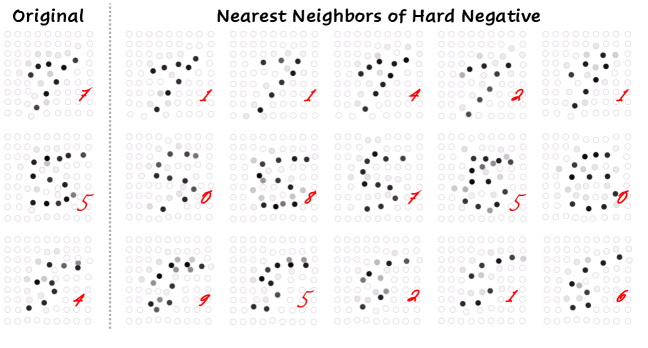
Figure 3: MNIST-superpixel graphs with their generated hard negatives’ nearest neighbors in the latent space. Red numbers indicate ground truth labels. The nearest neighbors of a sample’s hard negatives are typically similar to the sample while belonging to different classes.

By targeting critical dimensions identified through CKFI, Khan-GCL emphasizes essential semantic features, which significantly enhance its classification capabilities compared to existing hard negative integrated methods.

Nearest neighbors retrieval of the generated hard negatives.

To better elucidate the effectiveness of the generated hard negatives, we pre-train an encoder using Khan-GCL on MNIST-superpixel Monti et al. (2017), where handwritten digits from the MNIST dataset LeCun et al. (1998) are represented as graphs. During pre-training, we generate hard negatives for each graph and retrieve the nearest neighbors of each hard negative in the latent space across the entire dataset. We provide more details of this experiment in Appendix E. Figure 3 illustrates sample digit graphs alongside the five nearest neighbors of their corresponding hard negatives. The ground truth label for each graph is displayed in red at the bottom right corner. As shown in Figure 3, the nearest neighbors of a sample’s hard negatives typically exhibit structural similarity to the original sample while belonging to different classes. This observation confirms that forming negative pairs between a sample and such generated hard negatives effectively guides the encoder to discriminate between semantically similar samples from different classes, thereby enhancing the discriminative power of the learned encoder.

Table 3: Unsupervised learning performance (accuracy in %) for graph classification on TU-datasets, comparing Khan-GCL against existing hard negative integrated GCL methods. Benchmark results are from their corresponding original publications.

Datasets	DD	MUTAG	NCI1	PROTEINS	COLLAB	RDT-B	RDT-M5K	IMDB-B
AFANSWang et al. (2024)	-	90.0$\pm$1.0	80.4$\pm$0.5	75.4$\pm$0.5	74.7$\pm$0.5	91.1$\pm$0.1	-	-
ANGCLZhang et al. (2024b)	78.8$\pm$0.9	92.3$\pm$0.7	81.0$\pm$0.3	75.9$\pm$0.4	72.0$\pm$0.7	90.8$\pm$0.7	56.5$\pm$0.3	71.8$\pm$0.6
GraphACLLuo et al. (2023)	79.3$\pm$0.4	90.2$\pm$0.9	-	75.5$\pm$0.4	74.7$\pm$0.6	-	-	74.3$\pm$0.7
Khan-GCL(Ours)	80.6$\pm$0.7	91.4$\pm$1.1	80.8$\pm$0.9	76.9$\pm$0.8	75.2$\pm$0.3	92.2$\pm$0.3	56.9$\pm$0.5	75.0$\pm$0.4

5.2 Ablation Study

Effectiveness of the KAN encoder in Khan-GCL.

We conduct targeted experiments to evaluate the KAN encoder’s contribution to Khan-GCL’s performance. We evaluate a variant of Khan-GCL without CKFI and hard negative generation (denoted as ‘w/o hard neg.’ in Table 1 and Figure 4) and compare it with both the vanilla GCL method (GraphCL You et al. (2020), using an MLP encoder) and the complete Khan-GCL framework across transfer learning and unsupervised learning tasks. Results show that even without the hard negative generation, the ‘w/o hard neg.’ configuration consistently outperforms GraphCL, likely due to KAN’s better generalization power and its ability to mitigate inherent issues in deep GNNs like overfitting and over-smoothing. Furthermore, the integration of generated hard negatives in the complete Khan-GCL framework yields additional performance improvements over the ‘w/o hard neg.’ configuration, highlighting the benefits of our hard negative generation approach.

Effectiveness of two feature identification techniques in hard negative generation.

In this section, we evaluate the contributions of our two proposed critical feature identification techniques in hard negative generation. We introduce three variants of Khan-GCL: (1) ‘w/o d-dims’, where negatives are generated by perturbing only independent dimensions; (2) ‘w/o i-dims’, where perturbation is limited to discriminative dimensions; and (3) ‘w/ rand-perturb’, which generates negatives by applying random Gaussian noise across all dimensions. Detailed experimental settings for these configurations are provided in Appendix E. Figure 4 presents the performance of these configurations on unsupervised learning tasks. While ‘w/ rand-perturb’ yields performance improvements over the baseline (‘w/o hard neg.’) on several datasets, it occasionally results in performance degradation. Both specialized perturbation approaches (‘w/o d-dims’ and ‘w/o i-dims’) outperform the baseline, demonstrating the effectiveness of targeted feature identification technique. Additionally, Khan-GCL, which integrates both proposed feature identification techniques in CKFI, achieves the most substantial improvement and the best overall results, confirming the complementary nature of our dual feature identification approach.

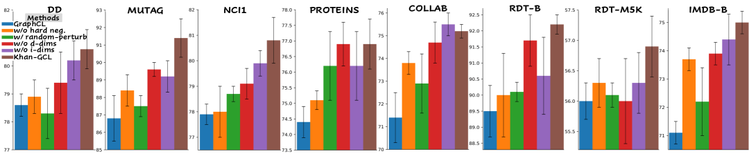
Figure 4: Ablation study results for Khan-GCL. Unsupervised learning results (in %) for graph classification on TU-datasets are shown.

6 Conclusion

We propose Khan-GCL, the first KAN-based graph contrastive learning framework, which balances expressive power and risks of inherent issues of deep GNNs by using a KAN-based encoder. We also introduce Critical KAN Feature Identification (CKFI) to identify key discriminative and independent features, enabling the generation of hard negatives through minimal perturbations. These hard negatives guide the encoder to learn more discriminative semantics during contrastive pre-training. Extensive experiments on biochemical and social network datasets demonstrate that our approach significantly improves generalization and transferability, achieving the state-of-the-art performance. Additional details and experimental results are provided in the Appendix.

For future work, exploring feature perturbation and hard negative generation in intermediate layers of a KAN encoder is promising. Further, reducing the additional training cost introduced by KAN’s spline computations through more efficient architectures is worth investigating.

Appendix

Appendix A Variance Bound of Uniform B-spline Function

We denote a uniform B-spline function $\phi(x)$ as:

$$\phi(x)=\sum_{k}c_{k}B_{k}(x)$$ (13)

Here $B_{k}(x)$ denotes the piecewise polynomial functions, and $c_{k}$ represents their corresponding coefficients. The mean of a B-spline function $\phi(x)$ is denoted by $\mu_{\phi}$, i.e.,

$$\mu_{\phi} =\frac{1}{b-a}\int_{a}^{b}\phi(x)dx=\frac{1}{b-a}\int_{a}^{b}\sum_{k}c_{k}B_{k}(x)dx=\frac{1}{b-a}\sum_{k}c_{k}\int_{a}^{b}B_{k}(x)dx$$ (14)

$$=\frac{1}{b-a}\sum_{k}c_{k}\omega_{k}$$

Let $\omega_{k}$ denote $\int_{a}^{b}B_{k}(x)dx$. When using uniform grids in the domain $(a,b)$ of $\phi(x)$, all $\omega_{k}$ share the same value $\omega$ for any $k$. And as uniform B-spline basis functions satisfy:

$$\sum_{k}B_{k}(x)=1\qquad\forall x$$ (15)

Integral both side of Equation 15:

$$\sum_{k}\int_{a}^{b}B_{k}(x)dx=\int_{a}^{b}1dx=b-a$$ (16)

For uniform B-spline, we thus have:

$$\omega=\frac{b-a}{n}$$ (17)

Here $n$ represent the number of coefficients. Plugging Equation 17 into Equation 14, we get:

$$\mu_{\phi}=\frac{1}{b-a}\sum_{k}c_{k}\omega_{k}=\frac{1}{n}\sum_{k}c_{k}=\bar{c}$$ (18)

The mean of coefficients $\{c_{k}\}$ is denoted by $\bar{c}$.

Therefore, the variance of $\phi(x)$ can be written as:

$$\mathrm{Var}[\phi(x)] =\int(\phi(x)-\mu_{\phi})^{2}dx$$ (19)

$$=\int(\sum_{k}c_{k}B_{k}(x)-\bar{c})^{2}dx$$

$$=\int(\sum_{k}c_{k}B_{k}(x)-\bar{c}\sum_{k}B_{k}(x))^{2}dx$$

$$=\int(\sum_{k}(c_{k}-\bar{c})B_{k}(x))^{2}dx$$

$$=\int\sum_{i}\sum_{j}(c_{i}-\bar{c})(c_{j}-\bar{c})B_{i}(x)B_{j}(x)dx$$

$$=\sum_{i}\sum_{j}(c_{i}-\bar{c})(c_{j}-\bar{c})\int B_{i}(x)B_{j}(x)dx$$

We use the following notation:

$$M_{ij} =\int B_{i}(x)B_{j}(x)dx$$ (20)

$$d_{i} =c_{i}-\bar{c}$$

Then Equation 19 can be expressed as:

$$\mathrm{Var}[\phi(x)]=\mathbf{d}^{T}\mathbf{M}\mathbf{d}$$ (21)

where $\mathbf{M}=[M_{ij}]$ and $\mathbf{d}=[d_{i}]$ are a matrix and a vector, respectively.

Although the following derivation is applicable to B-spline functions of any order, as we used cubic (third-order) B-splines throughout our implementations, we present it for cubic B-splines. In the case of a uniform cubic B-spline, $B_{k}(x)$ overlaps non-zero with at most 3 neighbors on each side (indices $k\pm 1$, $k\pm 2$, $k\pm 3$). As a result, $M_{ij}=0$ for $|i-j|>3$. We can denote the distinct overlap integrals by $M(0)$ for $i=j$, $M(1)$ for $|i-j|=1$, $M(2)$ for $|i-j|=2$, and $M(3)$ for $|i-j|=3$ (with $M(k)=0$ for $k\geq 4$). The matrix $\mathbf{M}$ can be written as:

$$\mathbf{M}=\begin{bmatrix}M(0)&M(1)&M(2)&M(3)&0&\cdots&0\\ M(1)&M(0)&M(1)&M(2)&M(3)&\cdots&0\\ M(2)&M(1)&M(0)&M(1)&M(2)&\cdots&0\\ M(3)&M(2)&M(1)&M(0)&M(1)&\cdots&0\\ 0&M(3)&M(2)&M(1)&M(0)&\cdots&0\\ \vdots&\vdots&\vdots&\vdots&\vdots&\ddots&\vdots\\ 0&0&0&0&0&\cdots&M(0)\end{bmatrix}$$ (22)

Then we can express $\mathrm{Var}[\phi(x)]$ as:

$$\mathrm{Var}[\phi(x)]=M(0)\sum_{i}d_{i}^{2}+2M(1)\sum_{i}d_{i}d_{i+1}+2M(2)\sum_{i}d_{i}d_{i+2}+2M(3)\sum_{i}d_{i}d_{i+3}$$ (23)

As $M(k)\geq 0$ for any $k\in\{0,1,2,3\}$, we have:

$$\mathrm{Var}[\phi(x)]\leq M(0)\sum_{i}d_{i}^{2}=M(0)\sum_{i}(c_{i}-\bar{c})^{2}=M(0)\sigma_{c}^{2}$$ (24)

Appendix B Higher-order Singular Value Decomposition

In Algorothm 1, we present the detailed process of Higher-Order Singular Value Decomposition (HOSVD), also known as Tucker Decomposition Tucker [1966], De Lathauwer et al. [2000]. For each 3-way coefficient tensor $\mathbfcal{C}\in\mathbb{R}^{n_{in}\times n_{out}\times n_{c}}$ within the KAN layer architecture, HOSVD produces a decomposition consisting of:

1. A core tensor $\mathbfcal{G}\in\mathbb{R}^{r_{1}\times r_{2}\times r_{3}}$, and

2. Three orthogonal basis matrices $\mathbf{U}^{(1)}\in\mathbb{R}^{n_{in}\times r_{1}}$, $\mathbf{U}^{(2)}\in\mathbb{R}^{n_{out}\times r_{2}}$, and $\mathbf{U}^{(3)}\in\mathbb{R}^{n_{c}\times r_{3}}$.

Each factor matrix $\mathbf{U}^{(k)}$ contains the leading $r_{k}$ left singular vectors obtained from the SVD of the mode-$k$ unfolding of tensor $\mathcal{C}$. These truncated orthonormal bases preserve the most significant components of the original tensor while enabling substantial parameter reduction.

Algorithm 1 Higher-Order Singular Value Decomposition (Tucker Decomposition).

Input: An $I$-way tensor $\mathbfcal{C}$.

for $i=1$ to $I$ do

  $\mathbf{C}^{i}$ = Unfold ($\mathbfcal{C},i$), # Unfold the tensor along the $\rm i^{th}$ mode.

  $\mathbf{U}^{(i)}$, $\mathbf{\Sigma}^{(i)}$, $\mathbf{V}^{(i)}$ = SVD ($\mathbf{C}^{i}$), # Perform singular value decomposition on the reshaped tensor.

  $\mathbf{U}^{(i)}=\mathbf{U}^{(i)}[:,:r_{i}]$ # Save the truncated singular vectors $\mathbf{U}^{(i)}$ as the model-i basis.

end for

$\mathbfcal{G}=\mathbfcal{C}$, # Initialize the tensor core with the $I$-way tensor $\mathbfcal{C}$.

for $i=1$ to $I$ do

  $\mathbfcal{G}$ = $\mathbfcal{G}\times_{i}(\mathbf{U}^{(i)})^{T}$, # Multiply the core tensor by the $\rm i^{th}$ orthogonal basis.

end for

Output: Core tensor $\mathbfcal{G}$, orthogonal basis $\mathbf{U}^{(1)}$, $\mathbf{U}^{(2)}$, $\cdots$, $\mathbf{U}^{(I)}$.

Appendix C Algorithm of Independent Feature Identification

In Algorithm 2, we present the detailed algorithm of our proposed independent feature identification technique in Critical KAN Feature Identification (CKFI).

Algorithm 2 Algorithm flow of independent feature identification.

Input: coefficient $\mathbfcal{C}\in\mathbb{R}^{d_{in}\times d_{out}\times d_{c}}$ of a KAN layer.

for $i=1$ to $d_{c}$ do

  $\mathbfcal{C}^{(-j)}=\mathbfcal{C}_{:,\{1,\dots,d_{out}\}\setminus\{i\},:},$ # $j_{th}$ mode-$2$ slice removed from $\mathbfcal{C}$.

  $\mathbfcal{G},\mathbf{U}^{(1)},\mathbf{U}^{(2)},\mathbf{U}^{(3)}=\mathrm{HOSVD}(\mathbfcal{C}^{(-j)})$ # Call Algorithm 1 to decompose $\mathbfcal{C}^{(-j)}$.

  $\mathbfcal{P}=\mathbfcal{G}\times_{1}\mathbf{U}^{(1)}\times_{2}\mathbf{I}\times_{3}\mathbf{U}^{(3)}$ # $\mathbfcal{P}$ is a partially reconstructed $\mathbfcal{C}^{(-j)}$.

  $\tilde{\mathbf{M}}^{(2)}=\mathrm{arg}\min_{\tilde{\mathbf{M}}^{(2)}}\|\mathbfcal{C}_{:,i,:}-\sum_{s=1}^{r_{2}}\tilde{M}_{s}^{(2)}\mathbfcal{P}_{:,s,:}\|_{F}^{2}$ # Project the missing slice back to the basis to get $\tilde{\mathbf{M}}^{(2)}=\{\tilde{M}_{s}^{(2)}\}$ by solving the least-squares.

  $\tilde{\mathbf{U}}^{(2)}_{i}=[\mathbf{U}^{(2)}_{1},\dots,\mathbf{U}^{(2)}_{i-1},\tilde{\mathbf{M}}^{(2)},\mathbf{U}^{(2)}_{i+1}\dots]$ # Plug $\tilde{\mathbf{M}}^{(2)}$ to $\mathbf{U}^{(2)}$.

  $\tilde{\mathbfcal{C}}_{j}=\mathbfcal{G}\times_{1}\mathbf{U}^{(1)}\times_{2}\tilde{\mathbf{U}}_{j}^{(2)}\times_{3}\mathbf{U}^{(3)}$ # Reconstruct $\mathbfcal{C}$.

  $\delta_{j}=\|\tilde{\mathbfcal{C}}_{j}-\mathbfcal{C}\|_{F}$ # Reconstruction error.

end for

Output: reconstruction error $\bm{\delta}=\{\delta_{i}\}$.

Appendix D Algorithm of Khan-GCL

In Algorithm 3, we conclude the algorithm flow of our proposed Khan-GCL pre-training approach in Pytorch-like Paszke [2019], Fey and Lenssen [2019] style.

Algorithm 3 Algorithm flow of Khan-GCL (Pytorch-like style).

Input: Initial KAN encoder parameters $\bm{\theta_{e}}$; Initial projection head parameters $\bm{\theta_{p}}$; Unlabeled dataloader; Hyperparameters $\epsilon_{\delta}$, $\epsilon_{\rho}$,$\sigma_{\rho}$,$\sigma_{\delta}$.

for $\mathrm{x}^{0}$ in $\mathrm{dataloader}$ do

   ^′′′Representations of augmented graphs in a mini-batch^′′′

  $\mathrm{x}^{\prime},\mathrm{x}^{\prime\prime}=\mathrm{A}_{1}(\mathrm{x}^{0}),\mathrm{A}_{2}(\mathrm{x}^{0})$

  $\mathrm{z}^{\prime},\mathrm{z}^{\prime\prime}=\mathrm{encoder}(\mathrm{x}^{\prime}),\mathrm{encoder}(\mathrm{x}^{\prime\prime})$

   ^′′′Identify critical dimensions and calculate perturbations^′′′

  $\mathrm{delta}=\mathrm{independent\_score}(\theta_{e})$ # See Algorithm 2 and Section 4.2.1 for details.

  $\mathrm{rho}=\mathrm{discriminative\_score}(\theta_{e})$ # See Section 4.2.2 for details.

  $\mathrm{alpha}=\mathrm{rademacher}(0.5)$ # rademacher distribution can be implemented by pytorch built-in

              function like torch.rand.

  $\mathrm{p_{\delta}},\mathrm{p_{\rho}}=\mathrm{normal}(\mathrm{mean}=\epsilon_{\delta}*\mathrm{delta},\mathrm{std}=\sigma_{\delta}),\mathrm{normal}(\mathrm{mean}=\epsilon_{\rho}*\mathrm{rho},\mathrm{std}=\sigma_{\rho})$

  $\mathrm{z_{hard}}^{\prime}=\mathrm{z}^{\prime}+\mathrm{alpha}*(\mathrm{p_{\rho}}+\mathrm{p_{\delta}})$

  $\mathrm{alpha}=\mathrm{rademacher}(0.5)$

  $\mathrm{p_{\delta}},\mathrm{p_{\rho}}=\mathrm{normal}(\mathrm{mean}=\epsilon_{\delta}*\mathrm{delta},\mathrm{std}=\sigma_{\delta}),\mathrm{normal}(\mathrm{mean}=\epsilon_{\rho}*\mathrm{rho},\mathrm{std}=\sigma_{\rho})$

  $\mathrm{z_{hard}}^{\prime\prime}=\mathrm{z}^{\prime\prime}+\mathrm{alpha}*(\mathrm{p_{\rho}}+\mathrm{p_{\delta}})$

   ^′′′Project to V space by projection head^′′′

  $\mathrm{v}^{\prime},\mathrm{v}^{\prime\prime},\mathrm{v_{hard}}^{\prime},\mathrm{v_{hard}}^{\prime\prime}=\mathrm{proj}(\mathrm{z}^{\prime}),\mathrm{proj}(\mathrm{z}^{\prime\prime}),\mathrm{proj}(\mathrm{z_{hard}}^{\prime}),\mathrm{proj}(\mathrm{z_{hard}}^{\prime\prime})$

   ^′′′Calculate loss and optimize networks^′′′

  $\mathrm{Loss\_CL}=\mathrm{contrast\_loss}(\mathrm{v}^{\prime},\mathrm{v}^{\prime\prime})$

  $\mathrm{Loss\_HN}=\mathrm{hn\_loss}(\mathrm{v}^{\prime},\mathrm{v_{hard}}^{\prime}.\mathrm{detach()})+\mathrm{hn\_loss}(\mathrm{v}^{\prime\prime},\mathrm{v_{hard}}^{\prime\prime}.\mathrm{detach()})$

  $\mathrm{Loss\_Khan}=\mathrm{Loss\_CL}+\mathrm{Loss\_HN}$

  $\mathrm{Loss\_Khan}.\mathrm{backward()}$

  $\mathrm{update}(\bm{\theta_{e}})$

  $\mathrm{update}(\bm{\theta_{p}})$

end for

Output: Pre-trained encoder parameters $\bm{\theta_{e}}$.

Appendix E Datasets and Evaluation Protocols

E.1 Datasets

We summarize the characteristics of all datasets utilized in our experiments in Table 4. For transfer learning experiments, we pre-train our encoder on Zinc-2M Sterling and Irwin [2015] and evaluate its performance across 8 datasets from MoleculeNet Wu et al. [2018]: BBBP, Tox21, SIDER, ClinTox, MUV, HIV, and BACE. In our unsupervised learning evaluations, we assess our method on 8 datasets from TU-datasets Morris et al. [2020], comprising NCI1, PROTEINS, DD, MUTAG, COLLAB, RDT-B, RDT-M5K, and IMDB-B. Additionally, we use MNIST-superpixel Monti et al. [2017] in our experiments.

Table 4: Details of datasets used in our experiments.

Datasets	Domain	Dataset size	Avg. node per graph	Avg. degree
Zinc-2M	Biochemical	2,000,000	26.62	57.72
BBBP	Biochemical	2,039	24.06	51.90
Tox21	Biochemical	7,831	18.57	38.58
SIDER	Biochemical	1,427	33.64	70.71
ClinTox	Biochemical	1,477	26.15	55.76
MUV	Biochemical	93,087	24.23	52.55
HIV	Biochemical	41,127	25.51	54.93
BACE	Biochemical	1,513	34.08	73.71
NCI1	Biochemical	4,110	29.87	1.08
PROTEINS	Biochemical	1,113	39.06	1.86
DD	Biochemical	1,178	284.32	715.66
MUTAG	Biochemical	188	17.93	19.79
COLLAB	Social Networks	5,000	74.49	32.99
RDT-B	Social Networks	2,000	429.63	1.16
RDT-M5K	Social Networks	4,999	508.52	1.17
IMDB-B	Social Networks	1,000	19.77	96.53
MNIST-superpixel	Superpixel	70,000	70.57	8

E.2 Evaluation Protocols

In this section, we present the tasks for evaluating our self-supervised learning framework. Detailed hyperparameters of these tasks are provided in Appendix F.

Transfer learning.

First, we pre-train the encoder on a large biochemical dataset Zinc-2M Sterling and Irwin [2015] using our proposed Khan-GCL framework. After pre-training, we discard the projection head and append a linear layer after the pre-trained encoder. Then we perform end-to-end fine-tuning of the encoder and linear layer on the training sets of the downstream datasets. Test ROC-AUC at the best validation epoch is reported. Each downstream experiment is performed 10 times, and the mean and standard deviation of ROC-AUC are reported. We refer to Hu et al. [2019] and You et al. [2020] for more details of this task.

Unsupervised learning.

In this task, we follow the setup of Sun et al. [2019]. Specifically, we pre-train the encoder on TU-datasets Morris et al. [2020]. While evaluating the encoder, we use a SVM classifier to classify the output representations of the encoder. We report 10-fold cross validation accuracy averaged for 5 runs.

More configurations of Khan-GCL in unsupervised learning.

In Section 5.2, to perform ablation study regarding CKFI and the hard negative generation approach, we introduce three additional configurations of Khan-GCL, i.e., ‘w/ random-perturb’, ‘w/o d-dims’, and ‘w/o i-dims’. Here we provide details of these three configurations.

1. ‘w/ random-perturb’: perturbations are sampled from random Gaussian distribution, i.e., for a graph representation $\mathbf{z}_{j}$, $\mathbf{z}_{j}^{hard}=\mathbf{z}_{j}+\mathbf{p}^{rand}$, where $\mathbf{p}^{rand}$ is sampled as follows:

   $$\mathbf{p}^{rand}=\{p_{i}^{rand}=\alpha_{i}\cdot u_{i}^{rand}:u_{i}^{rand}\sim\mathcal{N}(\epsilon_{rand},\sigma^{2}_{rand}),\alpha_{i}\sim\mathrm{Rademacher}(0.5)\}$$

2. ‘w/o d-dims’: perturbations are applied only to the independent dimensions, i.e., for a graph representation $\mathbf{z}_{j}$, $\mathbf{z}_{j}^{hard}=\mathbf{z}_{j}+\mathbf{p}^{\delta}$

3. ‘w/o i-dims’: perturbations are applied only to the discriminative dimensions, i.e., for a graph representation $\mathbf{z}_{j}$, $\mathbf{z}_{j}^{hard}=\mathbf{z}_{j}+\mathbf{p}^{\rho}$

MNIST-superpixel.

We follow the settings of You et al. [2020] in pre-training the encoder on MNIST-superpixel dataset Monti et al. [2017].

While performing nearest neighbor retrieval, for a certain graph $\mathbf{x}_{j}$ (whose representation is $\mathbf{z}_{j}$), we first generate a hard negative $\mathbf{z}_{j}^{hard}$ of it by applying the perturbations. Then we search the representations of all graphs across the dataset to find the 5 graphs with the largest latent similarity (measured by cosine similarity) with $\mathbf{z}_{j}^{hard}$.

Appendix F Detailed Experiment Settings

F.1 Encoder Architecture

For the sake of fairness across all comparison against existing methods, we follow You et al. [2020] for the input, output, and hidden layer size of the encoder. Details of the encoder are concluded in Table 5.

Table 5: Details of Model Architecture.

Experiments	Transfer Learning	Unsupervised Learning	MNIST-Superpixel
GNN Type	GIN	GIN	GIN
Encoder Neuron Number	[300,300,300,300,300]	[32,32,32]	[110,110,110,110]
Projection Head Neuron Number	[300,300]	[32,32]	[110,110]
Pooling Layer	Global Mean Pool	Global Add Pool	Global Add Pool

In Khan-GCL, we replace all MLPs in the encoder by same-sized KANs. In all implementations, we use cubic B-spline-based KANs where the grid sizes are set to 5.

F.2 Transfer Learning Settings

In transfer learning pre-training, we train the encoder using an Adam optimizer Kingma [2014] with initial learning rate $1\times 10^{-4}$ for 100 epochs. The temperature hyperparameter $\tau$ in contrastive loss is $0.1$. In hard negative generation, we choose $\epsilon_{\delta}=\epsilon_{\rho}=0.075$ and $\sigma_{\delta}=\sigma_{\rho}=0.05$.

F.3 Unsupervised Learning Settings

In unsupervised learning pre-training, the encoder is optimized by an Adam optimizer Kingma [2014] with initial learning rate $1\times 10^{-4}$ for 60 epochs. The temperature hyperparameter $\tau$ in contrastive loss is $0.2$. While generating perturbations, we choose $\epsilon_{\delta}=\epsilon_{\rho}=0.075$ and $\sigma_{\delta}=\sigma_{\rho}=0.05$.

Appendix G Training Time Comparison of KAN and MLP-based Encoder

All experiments are conducted on a single Nvidia A100 GPU. Table 6 compares the runtime of Khan-GCL with several state-of-the-art GCL approaches in Zinc-2M pre-training. Although the iterative computation involved in KAN’s B-spline functions incurs additional training overhead, Khan-GCL achieves a runtime comparable to recent state-of-the-art GCL approaches.

Table 6: Running time comparison.

Methods	GraphCL You et al. [2020]	RGCL Li et al. [2022]	Khan-GCL(Ours)
Time (second/iteration)	0.046	0.059	0.063

Appendix H Additional Experiment Results

H.1 MNIST-superpixel classification

In addition to the nearest neighbor retrieval experiment, we also present the classification accuracy of the pre-trained encoder on MNIST-superpixel in Table 7. After pre-training, the encoder is fine-tuned on 1% labeled data randomly sampled from the whole dataset.

Table 7: Performance comparison in MNIST-superpixel classification.

Methods	Infomax Sun et al. [2019]	GraphCL You et al. [2020]	RGCL Li et al. [2022]	Khan-GCL(Ours)
Acc (%)	63.2$\pm$0.8	83.4$\pm$0.3	83.8$\pm$0.4	84.2$\pm$0.3

H.2 Additional ablation study

In this section, we perform additional ablation studies on the hyperparameters $\epsilon_{\delta}$, $\epsilon_{\rho}$, $\sigma_{\delta}$, and $\sigma_{\rho}$ of Khan-GCL. Figure 5 presents the results of unsupervised learning on the PROTEINS dataset and averaged transfer learning performance with varying hyperparameter settings.

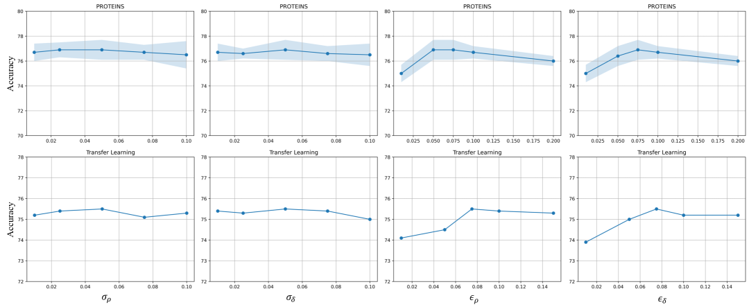
Figure 5: Ablation study results regarding hyperparameters.

Appendix I Potential Societal Impacts

By integrating expressive and interpretable Kolmogorov–Arnold Networks (KANs), Khan-GCL establishes a new state-of-the-art approach for self-supervised graph learning. This method is applicable to various real-world domains, including recommendation systems, cybersecurity, and drug discovery. We anticipate that leveraging KANs within GCL frameworks, along with our proposed feature identification techniques, will inspire further research in representation learning and self-supervised graph learning.

Nevertheless, since KAN architectures rely on iterative B-spline computations, they require more training time and computational resources compared to conventional MLPs. Consequently, this increased resource consumption may lead to environmental concerns, such as higher carbon emissions.

Appendix J Declaration of LLM usage

We used LLMs only for writing assistance, e.g., grammar and spell checking, and did not rely on them for generating or analyzing core research content.

References

- Ahmed and Sifat [2024] Tashin Ahmed and Md Habibur Rahman Sifat. Graphkan: Graph kolmogorov arnold network for small molecule-protein interaction predictions. In ICML’24 Workshop ML for Life and Material Science: From Theory to Industry Applications, 2024.
- Bresson et al. [2025] Roman Bresson, Giannis Nikolentzos, George Panagopoulos, Michail Chatzianastasis, Jun Pang, and Michalis Vazirgiannis. Kagnns: Kolmogorov-arnold networks meet graph learning, 2025. URL https://arxiv.org/abs/2406.18380.
- Chen et al. [2025] Jianfan Chen, Xuebiao Yuchi, Zhiwei Yan, Kejun Dong, and Hongtao Li. KA-GAT: Kolmogorov–arnold based graph attention networks, 2025. URL https://openreview.net/forum?id=zf777Odl6J.
- Chen et al. [2022] Tianlong Chen, Kaixiong Zhou, Keyu Duan, Wenqing Zheng, Peihao Wang, Xia Hu, and Zhangyang Wang. Bag of tricks for training deeper graph neural networks: A comprehensive benchmark study. IEEE Transactions on Pattern Analysis and Machine Intelligence, 45(3):2769–2781, 2022.
- Chen et al. [2020] Ting Chen, Simon Kornblith, Mohammad Norouzi, and Geoffrey Hinton. A simple framework for contrastive learning of visual representations. In International conference on machine learning, pages 1597–1607. PmLR, 2020.
- Chen et al. [2024] Yuzhou Chen, Jose Frias, and Yulia R Gel. Topogcl: Topological graph contrastive learning. In Proceedings of the AAAI conference on artificial intelligence, volume 38, pages 11453–11461, 2024.
- Cui et al. [2021] Ganqu Cui, Yufeng Du, Cheng Yang, Jie Zhou, Liang Xu, Xing Zhou, Xingyi Cheng, and Zhiyuan Liu. Evaluating modules in graph contrastive learning. arXiv preprint arXiv:2106.08171, 2021.
- Cybenko [1989] George Cybenko. Approximation by superpositions of a sigmoidal function. Mathematics of control, signals and systems, 2(4):303–314, 1989.
- De Lathauwer et al. [2000] Lieven De Lathauwer, Bart De Moor, and Joos Vandewalle. A multilinear singular value decomposition. SIAM journal on Matrix Analysis and Applications, 21(4):1253–1278, 2000.
- Fang et al. [2025] Taoran Fang, Tianhong Gao, Chunping Wang, Yihao Shang, Wei Chow, Lei Chen, and Yang Yang. Kaa: Kolmogorov-arnold attention for enhancing attentive graph neural networks, 2025. URL https://arxiv.org/abs/2501.13456.
- Fey and Lenssen [2019] Matthias Fey and Jan Eric Lenssen. Fast graph representation learning with pytorch geometric. arXiv preprint arXiv:1903.02428, 2019.
- Gao et al. [2021] Tianyu Gao, Xingcheng Yao, and Danqi Chen. Simcse: Simple contrastive learning of sentence embeddings. arXiv preprint arXiv:2104.08821, 2021.
- He et al. [2020] Kaiming He, Haoqi Fan, Yuxin Wu, Saining Xie, and Ross Girshick. Momentum contrast for unsupervised visual representation learning. In Proceedings of the IEEE/CVF conference on computer vision and pattern recognition, pages 9729–9738, 2020.
- Hornik et al. [1989] Kurt Hornik, Maxwell Stinchcombe, and Halbert White. Multilayer feedforward networks are universal approximators. Neural networks, 2(5):359–366, 1989.
- Hu et al. [2021] Qianjiang Hu, Xiao Wang, Wei Hu, and Guo-Jun Qi. Adco: Adversarial contrast for efficient learning of unsupervised representations from self-trained negative adversaries. In Proceedings of the IEEE/CVF Conference on Computer Vision and Pattern Recognition, pages 1074–1083, 2021.
- Hu et al. [2019] Weihua Hu, Bowen Liu, Joseph Gomes, Marinka Zitnik, Percy Liang, Vijay Pande, and Jure Leskovec. Strategies for pre-training graph neural networks. arXiv preprint arXiv:1905.12265, 2019.
- Ji et al. [2024] Qirui Ji, Jiangmeng Li, Jie Hu, Rui Wang, Changwen Zheng, and Fanjiang Xu. Rethinking dimensional rationale in graph contrastive learning from causal perspective. In Proceedings of the AAAI Conference on Artificial Intelligence, volume 38, pages 12810–12820, 2024.
- Kalantidis et al. [2020] Yannis Kalantidis, Mert Bulent Sariyildiz, Noe Pion, Philippe Weinzaepfel, and Diane Larlus. Hard negative mixing for contrastive learning. Advances in neural information processing systems, 33:21798–21809, 2020.
- Kiamari et al. [2024] Mehrdad Kiamari, Mohammad Kiamari, and Bhaskar Krishnamachari. Gkan: Graph kolmogorov-arnold networks, 2024. URL https://arxiv.org/abs/2406.06470.
- Kingma [2014] Diederik P Kingma. Adam: A method for stochastic optimization. arXiv preprint arXiv:1412.6980, 2014.
- LeCun et al. [1998] Yann LeCun, Léon Bottou, Yoshua Bengio, and Patrick Haffner. Gradient-based learning applied to document recognition. Proceedings of the IEEE, 86(11):2278–2324, 1998.
- Li et al. [2024a] Longlong Li, Yipeng Zhang, Guanghui Wang, and Kelin Xia. Ka-gnn: Kolmogorov-arnold graph neural networks for molecular property prediction, 2024a. URL https://arxiv.org/abs/2410.11323.
- Li et al. [2018] Qimai Li, Zhichao Han, and Xiao-Ming Wu. Deeper insights into graph convolutional networks for semi-supervised learning. In Proceedings of the AAAI conference on artificial intelligence, volume 32, 2018.
- Li et al. [2024b] Ruifeng Li, Mingqian Li, Wei Liu, and Hongyang Chen. Gnn-skan: Harnessing the power of swallowkan to advance molecular representation learning with gnns, 2024b. URL https://arxiv.org/abs/2408.01018.
- Li et al. [2022] Sihang Li, Xiang Wang, An Zhang, Xiangnan He, and Tat-Seng Chua. Let invariant rationale discovery inspire graph contrastive learning. In ICML, 2022.
- Li et al. [2025] Sihang Li, Yanchen Luo, An Zhang, Xiang Wang, Longfei Li, Jun Zhou, and Tat-Seng Chua. Self-attentive rationalization for interpretable graph contrastive learning. ACM Transactions on Knowledge Discovery from Data, 19(2):1–21, 2025.
- Liu et al. [2021] Shengchao Liu, Hanchen Wang, Weiyang Liu, Joan Lasenby, Hongyu Guo, and Jian Tang. Pre-training molecular graph representation with 3d geometry. arXiv preprint arXiv:2110.07728, 2021.
- Liu et al. [2024] Ziming Liu, Yixuan Wang, Sachin Vaidya, Fabian Ruehle, James Halverson, Marin Soljačić, Thomas Y Hou, and Max Tegmark. Kan: Kolmogorov-arnold networks. arXiv preprint arXiv:2404.19756, 2024.
- Luo et al. [2023] Xiao Luo, Wei Ju, Yiyang Gu, Zhengyang Mao, Luchen Liu, Yuhui Yuan, and Ming Zhang. Self-supervised graph-level representation learning with adversarial contrastive learning. ACM Transactions on Knowledge Discovery from Data, 18(2):1–23, 2023.
- Monti et al. [2017] Federico Monti, Davide Boscaini, Jonathan Masci, Emanuele Rodola, Jan Svoboda, and Michael M Bronstein. Geometric deep learning on graphs and manifolds using mixture model cnns. In Proceedings of the IEEE conference on computer vision and pattern recognition, pages 5115–5124, 2017.
- Morris et al. [2020] Christopher Morris, Nils M Kriege, Franka Bause, Kristian Kersting, Petra Mutzel, and Marion Neumann. Tudataset: A collection of benchmark datasets for learning with graphs. arXiv preprint arXiv:2007.08663, 2020.
- Oord et al. [2018] Aaron van den Oord, Yazhe Li, and Oriol Vinyals. Representation learning with contrastive predictive coding. arXiv preprint arXiv:1807.03748, 2018.
- Paszke [2019] A Paszke. Pytorch: An imperative style, high-performance deep learning library. arXiv preprint arXiv:1912.01703, 2019.
- Radford et al. [2021] Alec Radford, Jong Wook Kim, Chris Hallacy, Aditya Ramesh, Gabriel Goh, Sandhini Agarwal, Girish Sastry, Amanda Askell, Pamela Mishkin, Jack Clark, et al. Learning transferable visual models from natural language supervision. In International conference on machine learning, pages 8748–8763. PmLR, 2021.
- Rong et al. [2019] Yu Rong, Wenbing Huang, Tingyang Xu, and Junzhou Huang. Dropedge: Towards deep graph convolutional networks on node classification. arXiv preprint arXiv:1907.10903, 2019.
- Sterling and Irwin [2015] Teague Sterling and John J Irwin. Zinc 15–ligand discovery for everyone. Journal of chemical information and modeling, 55(11):2324–2337, 2015.
- Sun et al. [2019] Fan-Yun Sun, Jordan Hoffmann, Vikas Verma, and Jian Tang. Infograph: Unsupervised and semi-supervised graph-level representation learning via mutual information maximization. arXiv preprint arXiv:1908.01000, 2019.
- Suresh et al. [2021] Susheel Suresh, Pan Li, Cong Hao, and Jennifer Neville. Adversarial graph augmentation to improve graph contrastive learning. Advances in Neural Information Processing Systems, 34:15920–15933, 2021.
- Tucker [1966] Ledyard R Tucker. Some mathematical notes on three-mode factor analysis. Psychometrika, 31(3):279–311, 1966.
- Veličković et al. [2018] Petar Veličković, William Fedus, William L Hamilton, Pietro Liò, Yoshua Bengio, and R Devon Hjelm. Deep graph infomax. arXiv preprint arXiv:1809.10341, 2018.
- Wang et al. [2024] Shihao Wang, Chenxu Wang, Panpan Meng, and Zhanggong Wang. Afans: Augmentation-free graph contrastive learning with adversarial negative sampling. In International Conference on Intelligent Computing, pages 376–387. Springer, 2024.
- Wang et al. [2021] Yingheng Wang, Yaosen Min, Xin Chen, and Ji Wu. Multi-view graph contrastive representation learning for drug-drug interaction prediction. In Proceedings of the web conference 2021, pages 2921–2933, 2021.
- Wei et al. [2023] Chunyu Wei, Yu Wang, Bing Bai, Kai Ni, David Brady, and Lu Fang. Boosting graph contrastive learning via graph contrastive saliency. In International conference on machine learning, pages 36839–36855. PMLR, 2023.
- Wu et al. [2025] Ying Wu, Zhiyuan Zang, Xitao Zou, Wentao Luo, Ning Bai, Yi Xiang, Weiwei Li, and Wei Dong. Graph attention and kolmogorov–arnold network based smart grids intrusion detection. Scientific Reports, 15(1):8648, 2025. doi: 10.1038/s41598-025-88054-9. URL https://doi.org/10.1038/s41598-025-88054-9.
- Wu et al. [2018] Zhenqin Wu, Bharath Ramsundar, Evan N Feinberg, Joseph Gomes, Caleb Geniesse, Aneesh S Pappu, Karl Leswing, and Vijay Pande. Moleculenet: a benchmark for molecular machine learning. Chemical science, 9(2):513–530, 2018.
- Xia et al. [2021] Jun Xia, Lirong Wu, Ge Wang, Jintao Chen, and Stan Z Li. Progcl: Rethinking hard negative mining in graph contrastive learning. arXiv preprint arXiv:2110.02027, 2021.
- Xu et al. [2024] Jinfeng Xu, Zheyu Chen, Jinze Li, Shuo Yang, Wei Wang, Xiping Hu, and Edith C. H. Ngai. Fourierkan-gcf: Fourier kolmogorov-arnold network – an effective and efficient feature transformation for graph collaborative filtering, 2024. URL https://arxiv.org/abs/2406.01034.
- You et al. [2020] Yuning You, Tianlong Chen, Yongduo Sui, Ting Chen, Zhangyang Wang, and Yang Shen. Graph contrastive learning with augmentations. Advances in neural information processing systems, 33:5812–5823, 2020.
- You et al. [2021] Yuning You, Tianlong Chen, Yang Shen, and Zhangyang Wang. Graph contrastive learning automated. In International conference on machine learning, pages 12121–12132. PMLR, 2021.
- Zhang et al. [2024a] Bingxu Zhang, Changjun Fan, Shixuan Liu, Kuihua Huang, Xiang Zhao, Jincai Huang, and Zhong Liu. The expressive power of graph neural networks: A survey. IEEE Transactions on Knowledge and Data Engineering, 2024a.
- Zhang and Zhang [2024] Fan Zhang and Xin Zhang. Graphkan: Enhancing feature extraction with graph kolmogorov arnold networks, 2024. URL https://arxiv.org/abs/2406.13597.
- Zhang et al. [2024b] Qi Zhang, Cheng Yang, and Chuan Shi. Adaptive negative representations for graph contrastive learning. AI Open, 5:79–86, 2024b.
- Zhang et al. [2024c] Shichang Zhang, Ziniu Hu, Arjun Subramonian, and Yizhou Sun. Motif-driven contrastive learning of graph representations. IEEE Transactions on Knowledge and Data Engineering, 36(8):4063–4075, 2024c.
- Zhu et al. [2020] Yanqiao Zhu, Yichen Xu, Feng Yu, Qiang Liu, Shu Wu, and Liang Wang. Deep graph contrastive representation learning. arXiv preprint arXiv:2006.04131, 2020.
- Zhu et al. [2021] Yanqiao Zhu, Yichen Xu, Feng Yu, Qiang Liu, Shu Wu, and Liang Wang. Graph contrastive learning with adaptive augmentation. In Proceedings of the web conference 2021, pages 2069–2080, 2021.