Cost-aware LLM-based Online Dataset Annotation

Abstract

Recent advances in large language models (LLMs) have enabled automated dataset labeling with minimal human supervision. While majority voting across multiple LLMs can improve label reliability by mitigating individual model biases, it incurs high computational costs due to repeated querying. In this work, we propose a novel online framework, Cost-aware Majority Voting (CaMVo), for efficient and accurate LLM-based dataset annotation. CaMVo adaptively selects a subset of LLMs for each data instance based on contextual embeddings, balancing confidence and cost without requiring pre-training or ground-truth labels. Leveraging a LinUCB-based selection mechanism and a Bayesian estimator over confidence scores, CaMVo estimates a lower bound on labeling accuracy for each LLM and aggregates responses through weighted majority voting. Our empirical evaluation on the MMLU and IMDB Movie Review datasets demonstrates that CaMVo achieves comparable or superior accuracy to full majority voting while significantly reducing labeling costs. This establishes CaMVo as a practical and robust solution for cost-efficient annotation in dynamic labeling environments.

Keywords large language models (LLMs)  $\cdot$ dataset annotation  $\cdot$ optimization  $\cdot$ multi-armed bandits

1 Introduction

The rapid proliferation of data across domains has created an urgent need for accurate, large-scale annotation pipelines. While human experts and crowd workers have been the gold standard for dataset labeling, manual annotation is notoriously slow, expensive, and prone to inter-annotator inconsistency Petrović et al. (2020). As machine learning models become increasingly sophisticated, their demand for high-quality, richly labeled datasets only intensifies, exacerbating this bottleneck.

Recent advances in large language models (LLMs) offer a promising remedy: by leveraging transformer-based architectures such as GPT, it is now possible to automate much of the labeling workload. LLMs excel at natural-language understanding, reasoning, and contextual inference, enabling rapid generation of annotations with minimal human effort Naveed et al. (2023).

However, relying on a single LLM introduces issues of biases inherited from its training data and stochastic variability across repeated queries, undermining reliability and reproducibility Errica et al. (2024); Li et al. (2024a). A common strategy to bolster label quality is ensembling: querying multiple LLMs, or multiple samples from the same model, and aggregating their outputs via majority voting. This reduces hallucinations and offsets the bias of individual models but substantially increases cost, as each additional model increases latency and compute expenditure Yang et al. (2023). In practice, querying every available LLM for each instance is often wasteful and unnecessary.

In this paper, we address this trade-off by adaptively selecting a subset of LLMs for majority voting on each input, achieving comparable accuracy to full-ensemble voting while dramatically cutting cost. Unlike prior work on LLM weight optimization or query routing—which presumes access to ground-truth labels or a pre-trained routing model Chen et al. (2024); Nguyen et al. (2024); Ding et al. (2024)—our method operates online, without any held-out training set or ground truth.

Our contributions are as follows:

1. Online formulation. To the best of our knowledge, this is the first work on LLM-based dataset labeling in which both vote weights and the queried subset of LLMs are adapted in real time, i.e. without relying on a pre-trained model or a dedicated training set.

2. Cost-aware Majority Voting (CaMVo). We propose CaMVo, an algorithm that combines a LinUCB-style contextual bandit with a Bayesian Beta-mixture confidence estimator. For each candidate LLM, CaMVo computes a lower confidence bound on its correctness probability given the input’s embedding, then selects the smallest-cost subset whose aggregated confidence exceeds a user-specified threshold $\delta$.

3. Empirical validation. Through experiments on the MMLU benchmark and the IMDB Movie Review dataset, we show that CaMVo matches or exceeds the accuracy of full majority voting (majority voting with all available LLMs) while significantly reducing the cost: on MMLU, CaMVo achieves higher accuracy with around $40\%$ lower cost; on IMDB, it attains only $0.17\%$ drop in accuracy while halving query expenditure.

1.1 Related Work

Ensembling and Majority Voting with LLMs.

Aggregating outputs from multiple LLMs (or repeated queries to a single LLM) via majority voting has become a popular strategy to boost annotation reliability. Chen et al. (2024) analyze the effect of repeated queries to a single model and observe a non-monotonic accuracy curve: performance improves initially but degrades beyond an optimal number of calls due to task heterogeneity. While additional LM calls enhance accuracy on easier queries, they may introduce noise or inconsistency that degrades performance on more challenging ones. To address this, the authors propose a scaling model that predicts the optimal number of LM calls required to maximize aggregate performance. Trad and Chehab (2024) compare re-querying and multi-model ensembles, showing that ensemble strategies are most effective when individual models or prompts exhibit comparable performance levels, and ensemble gains may diminish when individual model accuracies diverge.

Yang et al. (2023) propose a weighted majority-voting ensemble for medical QA, combining dynamic weight adjustment with clustering-based model selection. However, their approach relies on offline training data and focuses solely on improving accuracy, without accounting for the cost of querying. In contrast, our approach selects a cost-effective subset of heterogeneous LLMs online, without any pre-training.

LLM Query Routing.

Query routing addresses the problem of selecting a single LLM per query to optimize cost or latency under performance constraints. Nguyen et al. (2024) cast LLM selection as a contextual bandit problem, training offline on labeled data to learn a routing policy that maps query embeddings to a single optimal LLM under a total budget constraint of $b$. Ding et al. (2024) train a router to distinguish “easy” versus “hard” queries, sending easy tasks to local LLMs and hard ones to cloud APIs. Unlike these methods, our method operates in a fully online setting without access to labeled training data, updating the model dynamically during the labeling process. Moreover, rather than routing to a single LLM, we select a cost-efficient subset for majority voting.

Confidence Estimation in LLM Outputs.

Estimating model confidence can guide automatic label selection. Kadavath et al. (2022) explore how a language model’s own uncertainty estimates can serve as predictors of answer correctness, and find that the cumulative log-probability the model assigns to its generated token sequence correlates strongly with factual accuracy across diverse benchmarks. Li et al. (2024a) generate code multiple times and use output similarity as a proxy for confidence, choosing the most consistent result. While these works focus on self-consistency of a single model, we estimate a probabilistic lower bound on each LLM’s correctness via a Bayesian Beta-mixture model, incorporating both past performance and context.

Weighted Majority Voting.

Beyond simple voting, weighted schemes assign each annotator or model a reliability score such as the accuracy of the annotator, or the label confidence reported by the annotator. One notable approach is the GLAD model by Whitehill et al. (2009), which formulates weighted majority voting as a probabilistic inference problem over annotator expertise and task difficulty. GLAD jointly estimates per-annotator reliability and per-item ambiguity via a generative model, using an EM algorithm to infer the latent variables. Li and Yu (2014) introduce Iterative Weighted Majority Voting (IWMV) to aggregate noisy crowd labels by iteratively estimating worker reliability, and show it approaches the oracle Maximum A Posteriori (MAP) solution.

Crowdsourcing.

Rangi and Franceschetti (2018) utilize the bandits-with-knapsacks framework to dynamically estimate worker accuracy and allocate tasks in real time to maximize overall labeling quality within a budget. Another influential model is by Raykar et al. (2010), which jointly infers true labels and annotator reliabilities by modeling each worker’s confusion matrix. Through an expectation–maximization procedure, the method down-weights inconsistent annotators and yields more accurate aggregated labels without prior knowledge of worker quality. Our method parallels this online estimation but differs in that it leverages contextual embeddings and targets LLM ensembles rather than human annotators.

The comparison of our work with prior work is summarized in Table 1

Method	Ensemble Type	Pretrained	Online	Contextual
Ours (CaMVo)	Subset voting	No	Yes	Yes
Yang et al. (2023)	Weighted voting	Yes	No	Yes
Nguyen et al. (2024)	Single-model routing	Yes	No	Yes
Ding et al. (2024)	Single-model routing	Yes	No	Yes
Chen et al. (2024)	Re-querying	No	No	No
Li et al. (2024a)	Re-querying	No	No	Yes
Li and Yu (2014)	Crowd aggregation	No	Yes	No
Rangi and Franceschetti (2018)	Crowd assignment	No	Yes	No
Raykar et al. (2010)	Crowd aggregation	No	Yes	No

Table 1: Comparison of our work with prior ensemble and routing approaches.

2 Problem Statement

In this section, we formally define the problem setting, introduce the baseline algorithm, and provide some results that will be used by our proposed algorithm, which will be introduced in §3.

Consider an unlabeled dataset $\mathcal{D}=\{x_{1},x_{2},\ldots,x_{T}\}$, where each $x_{t}$ denotes a data instance (e.g., a text sample). Let there be a set $[K]$ of $K$ distinct large language models (LLMs), where each LLM $l_{i}$ is associated with a known cost per token $\rho_{i}$ and can be represented as a function $l_{i}:\mathcal{Q}\rightarrow\mathcal{R}$, mapping a query $q\in\mathcal{Q}$ to a response $r\in\mathcal{R}$. We denote the total number of possible labels for the dataset $\mathcal{D}$ as $M$. The objective in this setting is to assign a predicted label $\hat{y}_{t}\in[M]$ to each data instance $x_{t}$ by querying a subset of the available LLMs and aggregating their outputs. Labeling is performed sequentially, where each data instance $x_{t}$ is processed in round $t$. In each round, LLMs are queried independently of other LLMs and without memory of prior interactions (i.e., no context is preserved between rounds). Furthermore, all queries are made in a zero-shot setting, meaning that no task-specific fine-tuning or additional training data is used.

To serve as a baseline, we introduce the following weighted majority voting scheme. In this scheme, the predicted label $y_{t}$ for instance $x_{t}$ is determined by aggregating the votes of all $K$ LLMs using:

$$y_{t}=\arg\max_{m\in[M]}\sum_{i=1}^{K}\omega_{\text{def},i}(t)\cdot{\mathds{1}\left\{y_{i,t}=m\right\}},$$ (1)

where ${\mathds{1}\left\{\cdot\right\}}$ is the indicator function that returns 1 if the condition is true and 0 otherwise, and $y_{i,t}$ denotes the label outputted by LLM $l_{i}$ for instance $x_{t}$. Since the true label is not available in our setting, we use the empirical accuracy of model $l_{i}$ as the voting weight. Hence, $\omega_{\text{def},i}(t)=(\sum_{s=1}^{t-1}\mathbb{I}(y_{i,s}=y_{s}))/N_{i,t},$ where $N_{i,t}$ denotes the number of times LLM $l_{i}$ has been queried up to round $t$, and $y_{s}$ is the predicted label for round $s$. The pseudocode for this scheme, which we refer to as the baseline method, is provided in Algorithm 2 in Appendix C.

The goal is to label the dataset $\mathcal{D}$ in a cost-efficient manner by dynamically selecting a subset of LLMs for each data instance $x_{t}$. To facilitate this selection, we assume access to a model $\text{Emb}(\cdot)$ that generates a $d$-dimensional embedding $\mathbf{e}_{t}=\text{Emb}(x_{t})$ for $x_{t}$ in round $t$. This embedding serves as a representation of the instance and plays an analogous role to the context in a contextual bandit framework. Using this embedding, our approach, which will be introduced in § 3, estimates a lower bound on the probability that a given LLM $l_{i}$ will produce the correct label for $x_{t}$, and utilizes this bound to determine the subset of LLMs. The details for estimating this lower bound is given in § 3.

Naturally, selecting only a subset of LLMs rather than querying all available models may result in reduced labeling accuracy. To manage this trade-off, we introduce a user-defined parameter $\delta\in[0,1]$ that specifies the desired minimum relative confidence of the selected subset compared to the full majority vote using all $K$ LLMs. Let $L_{i,t}$ denote the lower confidence bound on the estimated probability that LLM $l_{i}$ correctly labels instance $x_{t}$ at round $t$. Our algorithm identifies the cost-minimizing subset of LLMs whose aggregated confidence, relative to that of the baseline method, satisfies the accuracy constraint imposed by $\delta$.

We will leverage the following result to estimate the confidence of the majority vote label based on the $L_{i,t}$ and $\omega_{i}(t)$ values when majority voting is performed over a subset $\mathcal{A}$ of LLMs.

Lemma 2.1.

Let $\omega_{i}$ denote the weight and $L_{i}$ the lower confidence bound on the correctness of the output from LLM $l_{i}$. Suppose the outputs of LLMs are conditionally independent given the data instance. Then, for a subset of LLMs $\mathcal{A}\subseteq[K]$, the lower bound on the probability that majority voting over the subset yields the correct label is given by

$$\delta_{\mathcal{A}}(\bm{L},\bm{\omega})=\sum_{\begin{subarray}{c}S\subseteq\mathcal{A}\\ \sum_{r\in S}\omega_{r}>\frac{W_{\mathcal{A}}}{2}\end{subarray}}\prod_{i\in S}L_{i}\prod_{j\in\mathcal{A}\setminus S}(1-L_{j}),$$ (2)

where $W_{\mathcal{A}}=\sum_{i\in\mathcal{A}}\omega_{i}$. Proof of this result is provided in Appendix A.

Finally, we introduce a user-specified parameter $k_{\min}$, which enforces a floor on the number of LLMs queried per instance. By requiring at least $k_{\min}$ votes in every round, this constraint further safeguards label quality—ensuring that no annotation is based on fewer than $k_{\min}$ model predictions.

The proposed Cost-aware Majority Voting (CaMVo) algorithm, which incorporates these results and user-defined parameters, is presented in §3.

3 The CaMVo Algorithm

We propose a novel algorithm, Cost-aware Majority Voting (CaMVo), for efficient dataset labeling with large language models (LLMs). CaMVo aims to select a cost-effective subset of LLMs for each input instance by leveraging contextual embeddings to estimate a lower confidence bound on the probability that each model will produce a correct label. These bounds are computed using a LinUCB-based framework (Li et al., 2010). Based on this information, CaMVo identifies a subset of LLMs such that the confidence of their weighted majority vote exceeds a user-specified threshold $\delta$. If no such subset exists, the algorithm defaults to querying all available models. The pseudo-code of CaMVo is provided in Algorithm 1, and consists of six main steps described below.

Algorithm 1 Cost-aware Majority Voting (CaMVo) Algorithm

1:Input: Set of LLMs $[K]$, cost per token $\rho_{i}$ for each LLM $i$, embedding model $\text{Emb}(\cdot)$, confidence threshold $\delta$, LinUCB regularization parameter $\lambda_{L}$, exploration parameter $\alpha$, regularization parameter $\lambda_{R}$

2:Initialize: $A_{i}\leftarrow\lambda_{L}I_{d},~\bm{b}_{i}\leftarrow 0_{d},~\forall i\in[K]$

3:for each round $t=1,2,\ldots,T$ do

4:  Get context vector: $\mathbf{e}_{t}\leftarrow\text{Emb}(x_{t})$

5:  for each LLM $i=1,2,\ldots,K$ do

6:   $q_{i,t}(\bm{e}_{t})\leftarrow\mathbf{e}_{t}^{\top}A_{i,t-1}^{-1}\bm{b}_{i,t-1}$

7:   $\theta_{i,t}(\bm{e}_{t})=q_{i,t}(\bm{e}_{t})-\alpha\sqrt{\mathbf{e}_{t}^{\top}A_{i,t-1}^{-1}\mathbf{e}_{t}}$

8:   $\bar{L}_{i,t}\leftarrow\text{Est}_{i}(\theta_{i,t}(\bm{e}_{t}))$

9:   $L_{i,t}\leftarrow\frac{\bar{L}_{i,t}\cdot N_{i,t}+\lambda_{R}\cdot\log(t+1)/2}{N_{i,t}+\lambda_{R}\cdot\log(t+1)}$

10:   $\omega_{i,t}\leftarrow\mu_{i,t-1}\cdot q_{i,t}(\bm{e}_{t})$

11:  end for

12:  $\mathcal{A}_{t}\leftarrow\text{Oracle}(\mathbf{L}_{t},\bm{\omega}_{t},\delta,k_{\min})$

13:  Query LLMs: $y_{i,t}=l_{i}(x_{t}),\ i\in\mathcal{A}_{t}$

14:  $y_{t}\leftarrow\arg\max_{m}\sum_{i\in\mathcal{A}_{t},y_{i,t}=m}\omega_{i}(t)$

15:  if $|\mathcal{A}_{t}|>1$ then

16:   for each LLM $i\in\mathcal{A}_{t}$ do

17:     $r_{i,t}\leftarrow{\mathds{1}\left\{y_{i,t}=y_{t}\right\}}$

18:     Update: $A_{i,t}\leftarrow A_{i,t-1}+\mathbf{e}_{t}\mathbf{e}_{t}^{\top}$

19:     Update: $\bm{b}_{i,t}\leftarrow\bm{b}_{i,t-1}+r_{i,t}\mathbf{e}_{t}$

20:     Update: $\mu_{i,t}\leftarrow\frac{\sum_{s=1}^{t}{\mathds{1}\left\{y_{i,s}=y_{s}\right\}}}{N_{i,t}}$

21:     Update the parameters of $\text{Est}_{i}$

22:   end for

23:  end if

24:end for

LinUCB-Based Confidence Estimation.

For each LLM $l_{i}$, CaMVo maintains a matrix $A_{i}\in\mathbb{R}^{d\times d}$ and vector $\bm{b}_{i}\in\mathbb{R}^{d}$, initialized as $A_{i}=\lambda_{L}I_{d}$, $\bm{b}_{i}=\bm{0}$, where $\lambda_{L}>0$ is a user-defined parameter. Given $\bm{e}_{t}=\text{Emb}(x_{t})$, the estimated confidence, and its confidence bound is computed as:

$$q_{i,t}(\bm{e}_{t})=\bm{e}_{t}^{\top}A_{i,t-1}^{-1}\bm{b}_{i,t-1},\quad C_{i,t}(\bm{e}_{t})=\alpha\sqrt{\bm{e}_{t}^{\top}A_{i,t-1}^{-1}\bm{e}_{t}},$$

From these, the lower confidence bound (LCB) of LLM confidence can be found as:

$$\theta_{i,t}(\bm{e}_{t})=q_{i,t}(\bm{e}_{t})-C_{i,t}(\bm{e}_{t}).$$

Bayesian Estimation of Label Correctness.

Given the inherent probabilistic nature of LLM outputs, the estimated confidence score may not reliably indicate the correctness of a label. To address this, we introduce a Bayesian estimator $\text{Est}_{i}(\cdot)$ that models the posterior probability that $l_{i}$’s prediction is correct, conditioned on this confidence. First, we define a latent variable $h_{i,t}=\mathds{1}\{y_{i,t}=y_{t}\}$, where $y_{t}$ is the assigned label. Note that ideally, the true label should be used instead of $y_{t}$, but since we do not have access to the true label, we instead use $y_{t}$. We model the conditional likelihood of $q_{i,t}(\bm{e}_{t})$, given the latent variable $h_{i,t}$, as a Beta-distributed random variable:

$$q_{i,t}(\bm{e}_{t})\mid h_{i,t}=1\sim\text{Beta}(\alpha_{i,1},\beta_{i,1}),\quad q_{i,t}(\bm{e}_{t})\mid h_{i,t}=0\sim\text{Beta}(\alpha_{i,0},\beta_{i,0}).$$

Further, to model $\mathbb{P}(h_{i,t}=1)$, we use the empirical historical accuracy of $l_{i}$, $\mu_{i,t-1}$, which captures the accuracy of LLM $l_{i}$ relative to the predicted labels up to round $t-1$. Similarly, $\mathbb{P}(h_{i,t}=0)=1-\mu_{i,t-1}$. Applying Bayes’ rule with these models, the posterior probability is modeled as:

$$\text{Est}_{i}(q)=\mathbb{P}(h_{i,t}=1\mid q)=\frac{\mu_{i,t-1}\cdot\text{Beta}_{i}(q;\alpha_{i,1},\beta_{i,1})}{\mu_{i,t-1}\cdot\text{Beta}_{i}(q;\alpha_{i,1},\beta_{i,1})+(1-\mu_{i,t-1})\cdot\text{Beta}_{i}(q;\alpha_{i,0},\beta_{i,0})},$$

We apply this estimator to $\theta_{i,t}(\bm{e}_{t})$, the LCB of the estimated LLM confidence as $\bar{L}_{i,t}=\text{Est}_{i}(\theta_{i,t}(\bm{e}_{t}))$ to encourage exploration under the UCB principle. Note that unlike traditional UCB-based methods that promote exploration via upper bounds, we use the LCB as it expands the size of the set of LLMs likely to satisfy the confidence threshold $\delta$.

Regularization.

In the absence of ground-truth labels, empirical accuracy estimates in majority voting can overfit, resulting in overconfident weights and biased aggregation. To address this issue, we regularize the LCB of the estimated confidence of LLM $l_{i}$ using Laplace smoothing:

$$L_{i,t}=\frac{\bar{L}_{i,t}\cdot N_{i,t}+\lambda_{R}\cdot\log(t+1)/2}{N_{i,t}+\lambda_{R}\cdot\log(t+1)}$$ (3)

where $\lambda_{R}>0$ is a user-defined regularization parameter that controls the strength of smoothing.

Subset Selection with Oracle.

We define the weight of LLM $l_{i}$ for majority voting as $\omega_{i,t}:=\mu_{i,t-1}\cdot q_{i,t}(\bm{e}_{t})$. This way the weights of LLMs reflect both their past performance, and also their expected performance for the current data instance. An Oracle is used to find the lowest cost subset whose label confidence is above the threshold $\delta$ using the computed $L_{i,t}$ and $\omega_{i,t}$ values of LLMs. Using Lemma 2.1, this can be expressed as

$$\mathcal{A}_{t}=\text{Oracle}(\mathbf{L}_{t},\bm{\omega}_{t},\delta,k_{\min}):=\arg\min_{\mathcal{A}}c_{\mathcal{A}}(t):\delta_{\mathcal{A}}(\mathbf{L}_{t},\bm{\omega}_{t})\geq\delta,~|\mathcal{A}|\geq k_{\min}$$ (4)

where $c_{\mathcal{A}}(t)=\sum_{i\in\mathcal{A}}\rho_{i}\cdot H_{i}(x_{t}),$ and $H_{i}(x_{t})$ is the token count of the query to the LLM $l_{i}$ for data instance $x_{t}$ under the tokenization method of LLM $l_{i}$. Since we expect only one token as output (which will be the label for the data instance $x_{t}$), we ignore the output tokens. Note that as in Lemma 2.1, we assume that the outputs of LLMs are conditionally independent given the data instance. Also note that if no such $\mathcal{A}$ exists, CaMVo defaults to querying all LLMs.

Label Assignment.

We query the LLMs in $\mathcal{A}_{t}$ and receive their responses. The label for $x_{t}$ can be assigned via weighted majority vote using $y_{t}=\arg\max_{m\in[M]}\sum_{i\in\mathcal{A}_{t}}\omega_{i}(t)\cdot{\mathds{1}\left\{y_{i,t}=m\right\}}$.

Parameter Updates.

If $|A_{i,t}|>1$, for each $l_{i}\in\mathcal{A}_{t}$, CaMVo updates $A_{i,t}$, $\bm{b}_{i,t}$, and $\mu_{i,t}$, which is the empirical mean accuracy, as:

$$A_{i,t}\leftarrow A_{i,t-1}+\bm{e}_{t}\bm{e}_{t}^{\top},\quad\bm{b}_{i,t}\leftarrow\bm{b}_{i,t-1}+r_{i,t}\bm{e}_{t},\quad\mu_{i,t}\leftarrow\frac{\sum_{s=1}^{t}\mathds{1}\{y_{i,s}=y_{s}\}}{N_{i,t}}$$

where $r_{i,t}=\mathds{1}\{y_{i,t}=y_{t}\}$. Note that parameters are not updated when $|A_{i,t}|=1$ as the reward will always be $1$ in that case. The Beta distribution parameters $(\alpha_{i,h},\beta_{i,h})$ can be updated via maximum likelihood estimation or a method-of-moments approximation based on the mean and variance of past confidence scores. These approaches are discussed in Appendix B.

4 Experiments

4.1 Experiments on the MMLU Dataset

We first evaluate CaMVo on the MMLU dataset Hendrycks et al. (2021a, b), a challenging multiple-choice benchmark spanning 57 diverse subjects including mathematics, U.S. history, law, and computer science. MMLU is well-suited to our setting, as it demands broad world knowledge and strong reasoning capabilities—conditions under which majority voting is particularly effective. To reduce computational cost, we restrict our evaluation to the test split, which contains 14,042 instances.

Models and setup.

We use the following LLMs: Claude 3 Sonnet and Haiku from Anthropic Anthropic (2024), GPT-4o, o3-mini, and o1-mini from OpenAI OpenAI (2024), and LLaMA-3.3 and LLaMA-3.1 from Meta Meta (2024). All models are queried using temperature 0.35 and top-$p=1$, where applicable. To extract contextual embeddings for CaMVo, we use the 384-dimensional sentence transformer all-MiniLM-L6-v2 Wang et al. (2020). For computational efficiency, we approximate the confidence $\delta_{\mathcal{A}}(\bm{L},\bm{\omega})$ using the cumulative distribution function of a Beta distribution. Further implementation details and experimental setup are provided in Appendix D.

Results.

Table 2 (Left) reports the accuracy and cost of individual LLMs, as well as two baselines: Majority Vote, which aggregates all LLMs using weights proportional to their true accuracy, and the Baseline Method, which corresponds to Algorithm 2. Cost corresponds to the average input token cost when labeling the dataset and is reported in dollars per million input tokens. Accuracy reflects the percentage of data instances correctly labeled. CaMVo’s performance under varying confidence thresholds $\delta$ and minimum vote counts $k_{\min}\in\{1,3\}$ is shown in Table 3. Note that we include $k_{\min}=3$ in our experiments as model parameters do not get updated when only a single LLM is queried, a scenario that can occur under $k_{\min}=1$. As a result, users may prefer to avoid setting $k_{\min}=1$. Moreover, for $k_{\min}=2$, the selected pair of LLMs will always yield a majority vote in favor of the LLM with the higher weight, limiting the informativeness of the voting outcome. The algorithm is configured with $\alpha=0.25$, $\lambda_{R}=1$, and $\lambda_{L}=1$. The Target Accuracy column reflects the minimum accuracy CaMVo must exceed to satisfy the threshold $\delta$, and is computed as $\delta\times\text{(Majority Vote Accuracy)}=\delta\times 88.18\%$.

From Table 2, we observe that among individual models, o3-mini achieves the highest accuracy at 85.92%, while Majority Vote attains 88.18% at a substantially higher cost of $9.14 per million tokens. The Baseline Method also matches this accuracy and cost. Table 3 shows that CaMVo consistently meets or exceeds the desired accuracy levels specified by $\delta$, across all settings of $k_{\min}$. From Table 3, it can be observed that CaMVo consistently satisfies all target accuracy levels defined by the confidence parameter $\delta$. Moreover, the accuracy and cost of CaMVo exhibit a predictable trade-off: as $\delta$ decreases, the cost of labeling decreases accordingly, while accuracy also declines in a controlled manner. This behavior highlights the flexibility of CaMVo in adapting to a wide range of practical scenarios with varying accuracy and budget constraints. Further, at $\delta=0.97$ and $k_{\min}=1$, CaMVo achieves 88.33% accuracy at a cost of only $7.18, outperforming both baselines in cost-efficiency. This improvement stems from CaMVo’s ability to dynamically select LLM subsets based on both global accuracy estimates and instance-specific contextual confidence.

We also observe that when $k_{\min}=3$, lowering $\delta$ below 0.85 has negligible effect on cost or accuracy. This occurs because CaMVo settles on the lowest-cost trio: LLaMA-3.3, LLaMA-3.1, and Claude-3.5; whose combined cost ($1.44) represents a lower bound given the constraint on $k_{\min}$.

LLM / Method	Accuracy (%)	Cost
o3-mini	85.92	1.10
claude-3-7-sonnet	85.65	3.00
o1-mini	84.82	1.10
gpt-4o	83.58	2.50
llama-3.3-70b	81.70	0.59
llama-3.1-8b	68.01	0.05
claude-3-5-haiku	64.09	0.80
Majority Vote	88.18	9.14
Baseline Method	88.18	9.14

LLM / Method	Accuracy (%)	Cost
gpt-4o	95.68	2.50
o3-mini	95.40	1.10
claude-3-5-haiku	95.05	0.80
gpt-4o-mini	94.60	0.15
o1-mini	94.52	1.10
llama-3.1-8b	94.06	0.05
llama-3.3-70b	92.23	0.59
Majority Vote	95.62	6.29
Baseline Method	95.61	6.29

Table 2: Accuracy and cost of individual LLMs and baseline ensemble methods on the MMLU dataset (Left), and the IMDB Movie Reviews Dataset (Right).

CaMVo $\delta$	Target Acc. (%)	Acc. (%) $k_{\min}=1$	Cost $k_{\min}=1$	Acc. (%) $k_{\min}=3$	Cost $k_{\min}=3$
0.99	87.30	88.47	9.14	88.47	9.14
0.98	86.42	88.59	8.57	88.59	8.57
0.975	85.98	88.49	7.80	88.49	7.80
0.97	85.53	88.35	6.67	88.33	6.67
0.965	85.09	88.27	5.66	88.27	5.66
0.96	84.65	87.98	4.74	88.03	4.74
0.955	84.21	87.40	3.38	87.01	3.36
0.95	83.77	86.82	2.76	87.01	2.96
0.90	79.36	84.88	1.19	84.80	1.81
0.85	74.95	84.41	1.03	82.14	1.58
0.80	70.54	82.12	0.70	81.32	1.51
0.75	66.14	68.80	0.16	81.24	1.50
0.70	61.73	68.38	0.14	81.22	1.50

Table 3: Accuracy and cost of CaMVo on the MMLU dataset under varying confidence thresholds $\delta$ and $k_{\min}\in\{1,3\}$. For reference, the cost of the baseline method is $9.14 per million tokens.

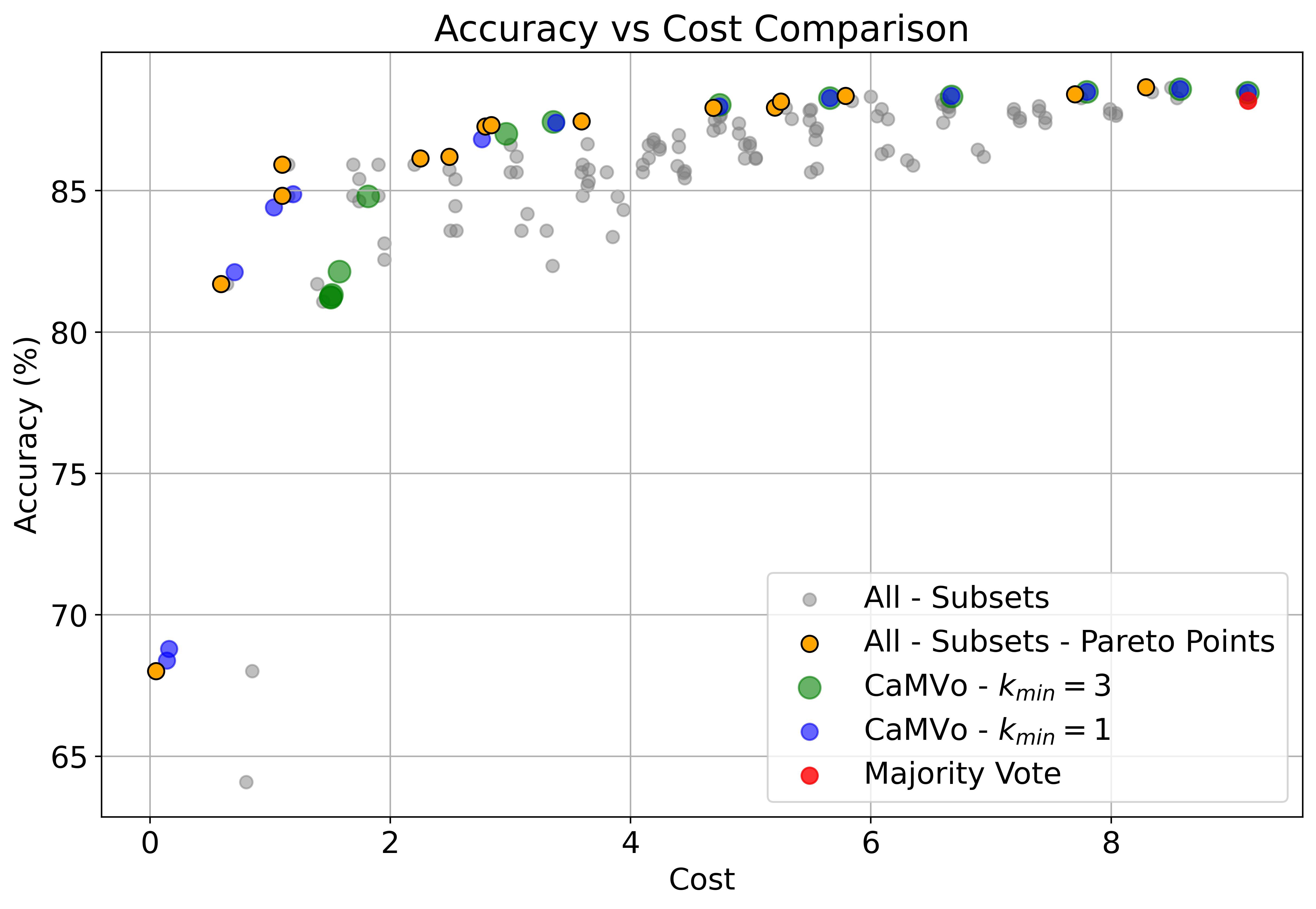
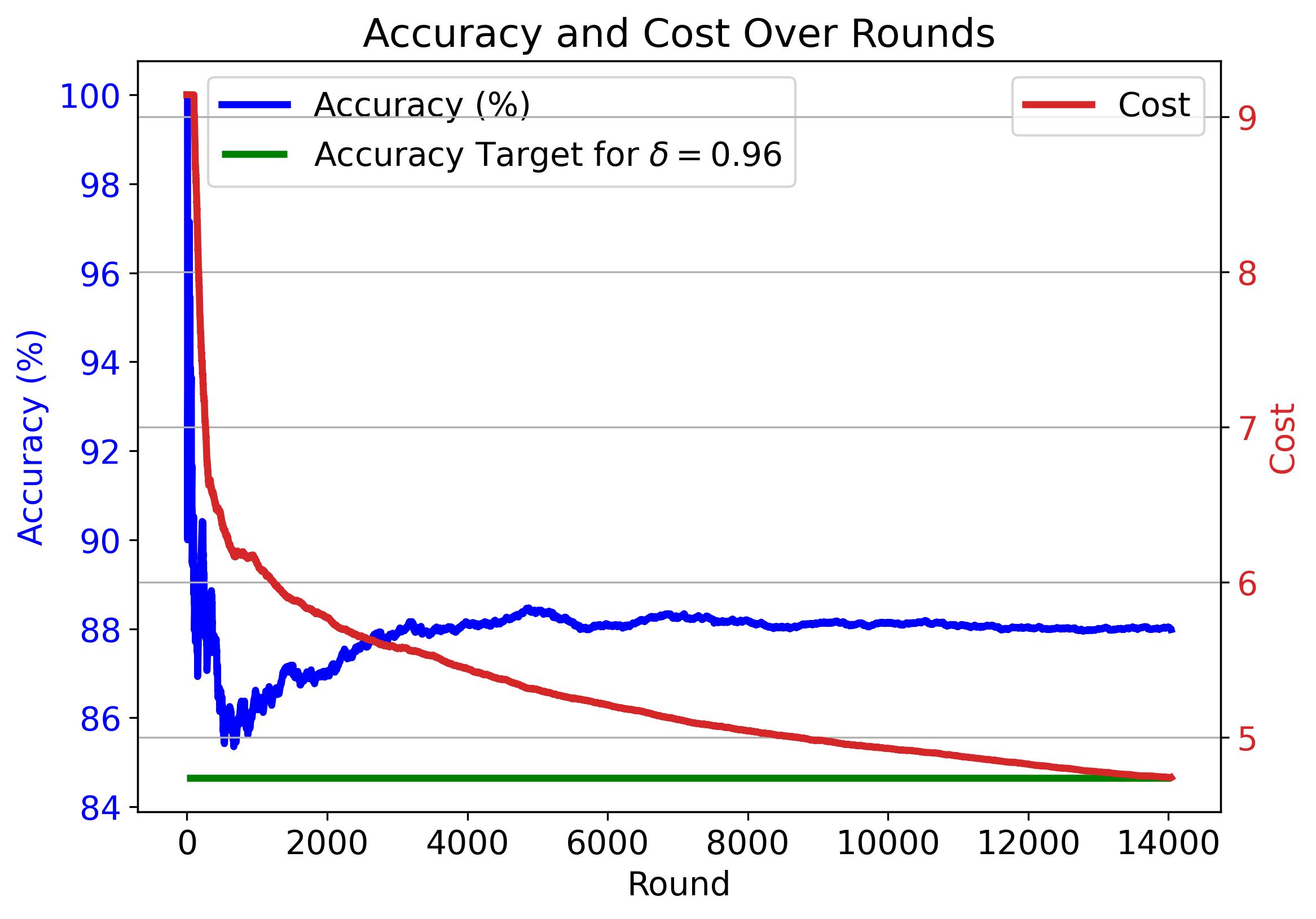
Figure 1: (Left) Cost–accuracy trade-off for MMLU dataset: gray dots show every LLM subset via weighted majority voting, yellow dots trace their Pareto-optimal frontier, blue markers are CaMVo at $k_{\min}=1$, green markers at $k_{\min}=3$, and the red marker denotes the Baseline Method. (Right) Cumulative average accuracy and cost of CaMVo with $\delta=0.96$, $k_{\min}=1$ over rounds.

Figure 1 (Left) illustrates the cost–accuracy trade-off of All Subsets versus CaMVo. Each gray point represents one of the $2^{K}\!-\!1$ possible LLM subsets voted via ground-truth accuracies, while the yellow curve depicts those that are Pareto-optimal. CaMVo’s results appear as blue markers for $k_{\min}=1$ and green markers for $k_{\min}=3$. The red marker denotes the Baseline Method. Remarkably, even without any a priori knowledge of LLM performance, or any pre-training, CaMVo consistently tracks, and sometimes surpasses the Pareto frontier, demonstrating its ability to approximate optimal cost–accuracy trade-offs in an online manner.

Figure 1 (Right) shows CaMVo’s cumulative average accuracy (blue) and cost (red) for $\delta=0.96$, $k_{\min}=1$; the green horizontal line indicates the target accuracy. In early rounds, CaMVo explores larger, more expensive subsets, yielding both high cost and high accuracy. As the LCB estimates converge, the algorithm rapidly shifts to smaller, cheaper subsets that still satisfy the accuracy threshold. Cost declines steeply while accuracy stabilizes just above the target, illustrating CaMVo’s ability to quickly identify and exploit the most cost-effective ensembles without sacrificing labeling quality. Additional plots with different parameters are provided in Appendix D.

4.2 Experiments on the IMDB Movie Reviews Dataset

We next test CaMVo on the IMDB Movie Reviews dataset Maas et al. (2011), a balanced binary-sentiment benchmark of 50,000 movie reviews. As before, we compare CaMVo against each individual LLM, a full-ensemble Majority Vote, and the Baseline Method (Algorithm 2).

Models and setup.

We employ Anthropic’s Claude 3-5 Haiku Anthropic (2024); OpenAI’s GPT-4o, o3-mini, GPT-4o-mini, and o1-mini OpenAI (2024); and Meta’s LLaMA-3.3 and LLaMA-3.1 Meta (2024). All queries use temperature = 0.25 and top-$p=1$, where applicable. We extract 384-dimensional contextual embeddings with all-MiniLM-L6-v2 Wang et al. (2020) and approximate the confidence bound $\delta_{\mathcal{A}}(\bm{L},\bm{\omega})$ via the Beta-CDF, as in §4.1.

Results.

Table 2 (Right) reports the accuracy and cost (in dollars per million input tokens) of each LLM and the two baselines. The baseline underperforms the best individual model (95.68% vs. 95.61%) despite incurring a significantly higher cost. This is partly due to the relative ease of the IMDB Movie Reviews dataset, where individual LLMs already achieve high accuracy, limiting the marginal benefit of ensembling. As noted by Li et al. (2024b), ensemble gains are most pronounced on harder tasks. Additionally, Trad and Chehab (2024) highlight that large performance gaps among models can reduce ensemble effectiveness, making smaller, selective subsets preferable in such cases.

Table 4 presents CaMVo’s accuracy–cost trade-off across various thresholds $\delta$ and $k_{\min}\in\{1,3\}$. CaMVo’s hyperparameters are $\alpha=0.7$, $\lambda_{R}=5$, and $\lambda_{L}=1$; and the Target Accuracy is computed similarly as $\delta\times 95.62\%$. Across all configurations, CaMVo meets or exceeds its target accuracy. Further, CaMVo achieves less than half the cost (when $\delta=0.997$ and $k_{\min}=1$) at a slightly lower accuracy of $95.45\%$ compared to the baseline, confirming its practicality for large-scale sentiment annotation without any pre-training or ground-truth labels.

CaMVo $\delta$	Target Acc. (%)	Acc. (%) $k_{\min}=1$	Cost $k_{\min}=1$	Acc. (%) $k_{\min}=3$	Cost $k_{\min}=3$
0.999	95.52	95.59	6.15	95.59	6.15
0.998	95.43	95.43	4.03	95.43	4.03
0.997	95.33	95.45	2.83	95.45	2.83
0.995	95.14	95.25	2.06	95.25	2.06
0.99	94.66	95.10	1.09	95.12	0.99
0.985	94.20	94.69	0.34	95.06	0.84
0.98	93.71	94.69	0.31	95.07	0.83
0.97	92.75	94.56	0.22	95.07	0.82
0.96	91.80	94.21	0.13	95.06	0.81
0.95	90.84	94.28	0.14	95.07	0.81
0.9	86.06	94.24	0.10	95.06	0.81

Table 4: Accuracy and cost of CaMVo on the IMDB dataset under varying confidence thresholds $\delta$ and $k_{\min}\in\{1,3\}$. For reference, the cost of the baseline method is $6.29 per million tokens.

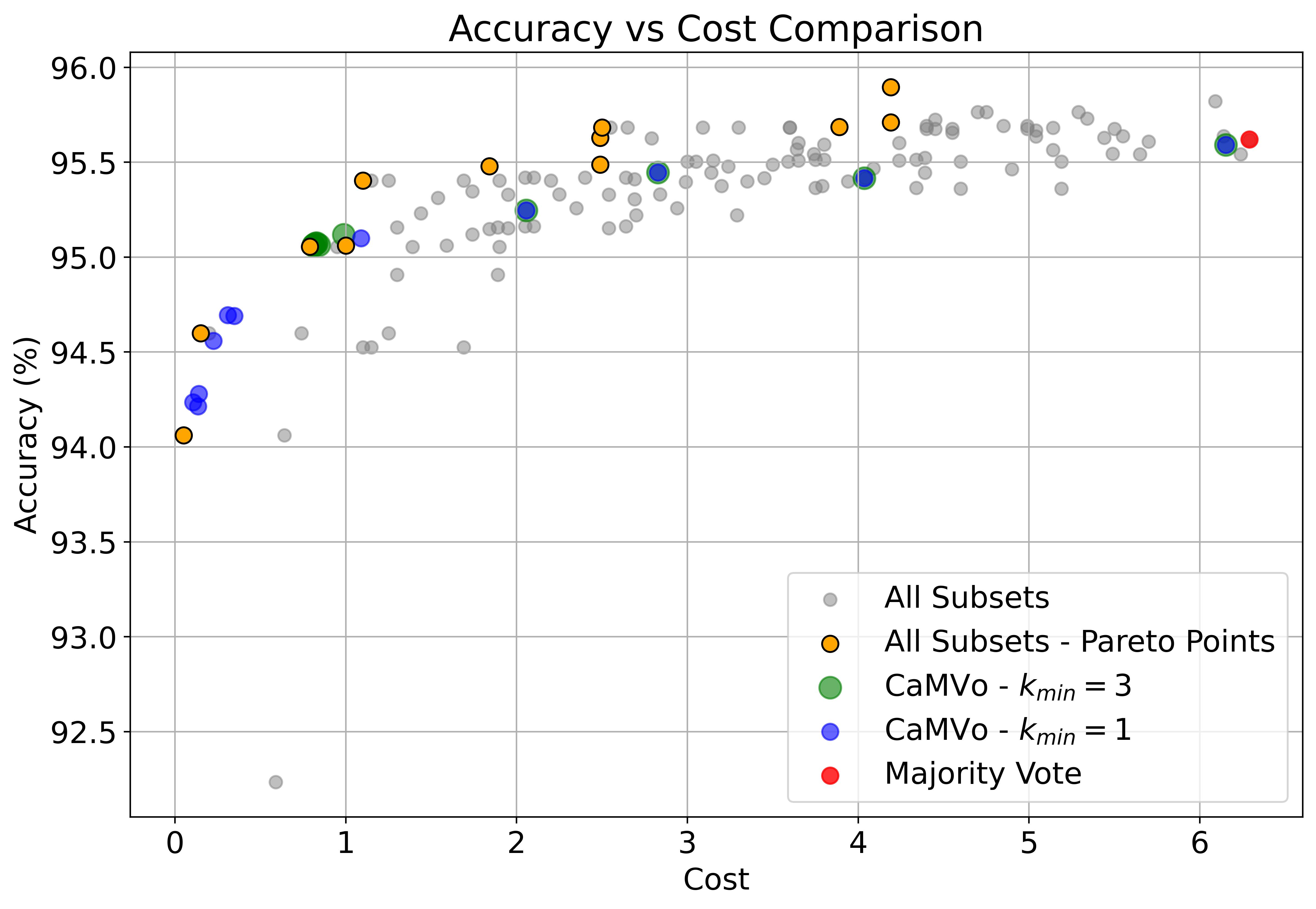
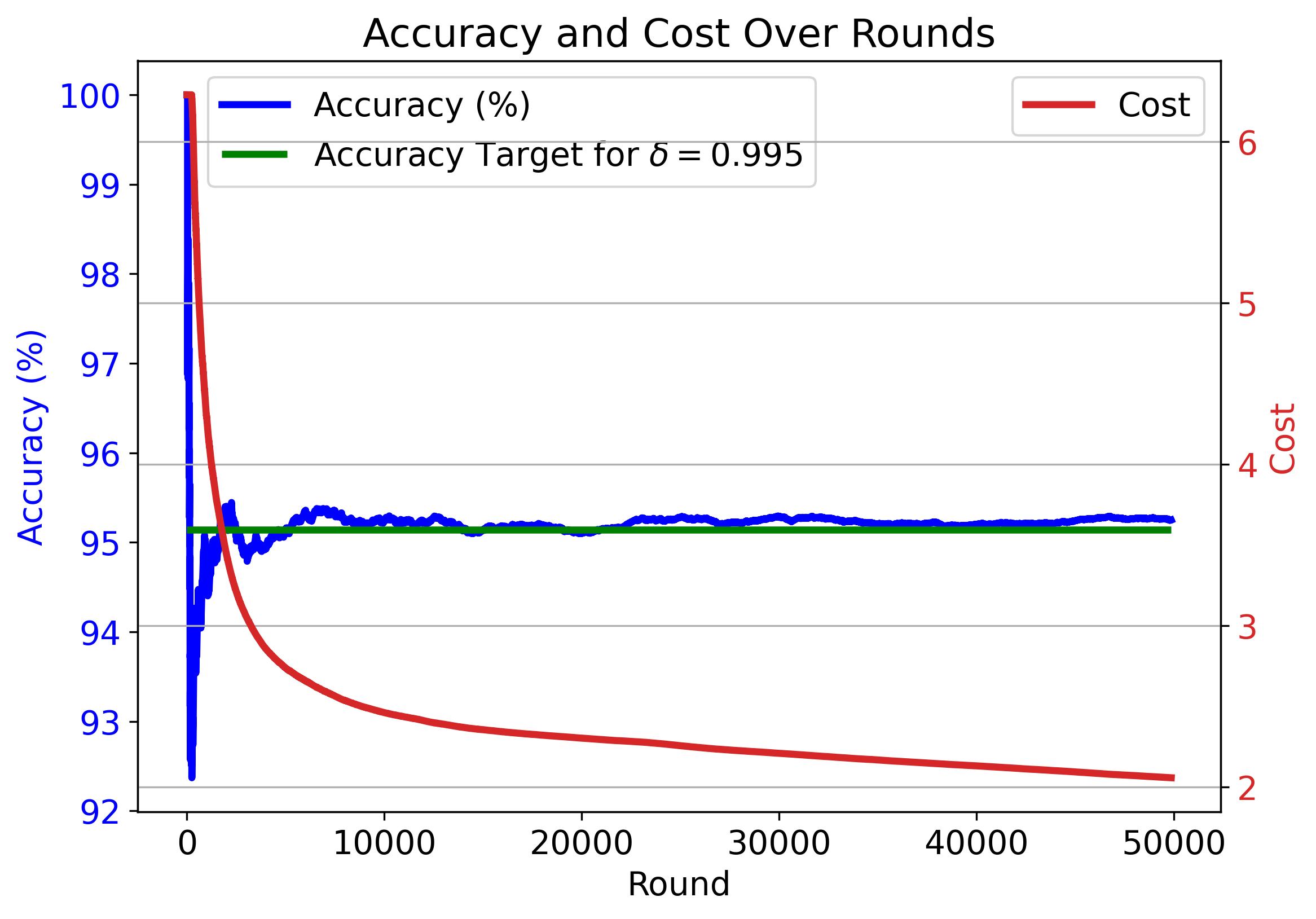
Figure 2: (Left) Cost–accuracy trade-off for IMDB dataset: gray dots show every LLM subset via weighted majority voting, yellow dots trace their Pareto-optimal frontier, blue markers are CaMVo at $k_{\min}=1$, green markers at $k_{\min}=3$, and the red marker denotes the Baseline Method. (Right) Empirical average accuracy and cost of CaMVo with $\delta=0.995$, $k_{\min}=1$ over rounds.

Figure 2 (Left) presents the analogous comparison of Figure 1 (Left) on the IMDB sentiment task. As before, gray points and the yellow Pareto-frontier points show all possible subset combinations, while blue and green markers plot CaMVo at $k_{\min}=1$ and $3$, respectively. The red marker denotes the Baseline Method. CaMVo closely matches the Pareto front in the low-cost regime (cost $<1$), but lags behind in higher-cost regions. This exposes a key limitation: when majority voting with additional LLMs is ineffective, CaMVo’s reliance on the independence assumption, which suggests that aggregating more LLMs improves accuracy; can lead to suboptimal performance.

Figure 2 (Right) plots CaMVo’s cumulative average accuracy (blue) and cost (red) on IMDB with $\delta=0.995$ and $k_{\min}=1$; the green line marks the target accuracy. As before, early rounds involve querying larger, costlier ensembles to robustly explore each model’s performance. Once the lower-confidence bounds stabilize, CaMVo swiftly transitions to minimal-cost subsets that still meet the accuracy requirement. This demonstrates CaMVo’s rapid convergence to cost-effective model combinations without compromising annotation quality. Additional results for other parameter settings appear in Appendix E.

5 Limitations

Our work relies on the assumption that the outputs of LLMs are independent of each other. Under this assumption, aggregating any subset of models with individual accuracy above $50\%$ strictly improves majority-vote performance. In practice; i.e., on the IMDB sentiment task (§4.2), LLM outputs can be highly correlated, and majority voting may underperform the best single model. Consequently, CaMVo inherits these failures and can yield lower ensemble accuracy when independence is violated. Nevertheless, even in such regimes CaMVo still achieves the user-specified accuracy threshold while reducing cost relative to the full-ensemble baseline. This is mostly due to the fact that our results are relative to the full-ensemble baseline which also suffers from the same issue. Extending CaMVo by accounting for inter-model correlations (e.g., via joint confidence estimation or diversity-aware selection) to better find the optimal subset is a promising and challenging direction for future work.

6 Conclusions

We have introduced Cost-aware Majority Voting (CaMVo), the first fully online framework for LLM-based dataset labeling that jointly adapts both vote weights and the subset of models queried on a per-instance basis. By combining a LinUCB-style contextual bandit with a Bayesian Beta-mixture confidence estimator, CaMVo estimates a lower bound on each LLM’s correctness probability for the given input and selects the minimal-cost ensemble that meets a user-specified accuracy threshold.

Empirical results on the MMLU and IMDB benchmarks demonstrate that CaMVo matches or exceeds full-ensemble majority-vote accuracy while reducing labeling cost. On MMLU, CaMVo even surpasses the true Pareto frontier of all possible weighted subsets—despite having no prior knowledge of individual model performance. These findings establish CaMVo as a practical solution for cost-efficient, automated annotation in dynamic labeling environments without any ground-truth labels or offline training.

Our analysis assumes independence among LLM outputs, which can be violated in practice and may degrade ensemble gains. Nonetheless, CaMVo still enforces the user’s accuracy target and delivers significant cost savings even under these conditions. Future work will explore diversity-aware selection and joint confidence models to mitigate correlated errors. We will also extend CaMVo to support iterative relabeling, allowing previously annotated instances to be revisited and refined as additional contextual information becomes available.

Appendix A Proof of Lemma 2.1

Proof.

Assume that each LLM $l_{i}\in\mathcal{A}$ produces a correct label with probability at least $L_{i}$, independently of other models. Define the random variable $Z_{i}\sim\text{Bernoulli}(L_{i})$ to represent whether model $l_{i}$ correctly labels the data instance, where $\mathbb{E}[Z_{i}]\geq L_{i}$. The total weight of LLMs that output the correct label is given by:

$$W_{C,\mathcal{A}}:=\sum_{i\in\mathcal{A}}\omega_{i}\cdot Z_{i},$$ (5)

and the total weight of all LLMs in $\mathcal{A}$ is:

$$W_{\mathcal{A}}:=\sum_{i\in\mathcal{A}}\omega_{i}.$$ (6)

Majority voting yields the correct label if the cumulative weight of correctly labeling LLMs exceeds half of the total weight, i.e. when

$$W_{C,\mathcal{A}}>\frac{W_{\mathcal{A}}}{2}.$$ (7)

Hence, $\delta_{\mathcal{A}}(\bm{L},\bm{\omega})$ can be expressed as

$$\delta_{\mathcal{A}}(\bm{L},\bm{\omega})=\mathbb{P}\left(W_{C,\mathcal{A}}>\frac{W_{\mathcal{A}}}{2}\right).$$ (8)

To compute this probability, we consider all possible label correctness outcomes for the subset $\mathcal{A}$. Let $S\subseteq\mathcal{A}$ denote the subset of LLMs that produce correct labels, while $\mathcal{A}\setminus S$ corresponds to those that produce incorrect labels. The probability of this joint outcome under the independence assumption is

$$\mathbb{P}_{S}(\bm{L},\bm{\omega})=\prod_{i\in S}L_{i}\prod_{j\in\mathcal{A}\setminus S}(1-L_{j}).$$ (9)

Summing over all subsets $S\subseteq\mathcal{A}$ for which the total weight of correctly labeling models exceeds half the total weight gives the desired result:

$$\delta_{\mathcal{A}}(\bm{L},\bm{\omega})=\sum_{\begin{subarray}{c}S\subseteq\mathcal{A}\\ \sum_{r\in S}\omega_{r}>\frac{W_{\mathcal{A}}}{2}\end{subarray}}\prod_{i\in S}L_{i}\prod_{j\in\mathcal{A}\setminus S}(1-L_{j}).$$ (10)

∎

Appendix B Estimating the Shape Parameters of the Beta Distribution

In this section, we present two methods for estimating the shape parameters of the Beta distributions used in CaMVo. The first is a maximum-likelihood estimation (MLE) approach that yields a closed-form system of equations, while the second is an efficient approximation based on the method of moments. Due to its computational practicality, the second method is used in our experiments.

Maximum-likelihood Estimation.

$\alpha_{i,1}$ and $\beta_{i,1}$ for the Beta distribution $\mathrm{Beta}_{i}(\alpha_{i,1},\beta_{i,1})$ corresponding to LLM $l_{i}$ can be estimated by maximizing the log-likelihood:

$$\ell_{i}(\alpha_{i,1},\beta_{i,1})=(\alpha_{i,1}-1)\sum_{s=1}^{t}\ln q_{i}(e_{s},s)+(\beta_{i,1}-1)\sum_{s=1}^{t}\ln(1-q_{i}(e_{s},s))-t\ln B(\alpha_{i,1},\beta_{i,1})$$ (11)

Taking derivatives with respect to $\alpha_{i,1}$ and $\beta_{i,1}$ and setting them to zero yields the MLE system:

$$\frac{\partial\ell_{i}}{\partial\alpha_{i,1}} =\sum_{s=1}^{t}\ln q_{i}(e_{s},s)-t\left(\psi(\alpha_{i,1})-\psi(\alpha_{i,1}+\beta_{i,1})\right)=0$$ (12)

$$\frac{\partial\ell_{i}}{\partial\beta_{i,1}} =\sum_{s=1}^{t}\ln(1-q_{i}(e_{s},s))-t\left(\psi(\beta_{i,1})-\psi(\alpha_{i,1}+\beta_{i,1})\right)=0$$ (13)

where $\psi(\cdot)$ is the digamma function $\psi(x)=\frac{d}{dx}\ln\Gamma(x)$. Solving this system yields the MLE estimates for the parameters of each LLM. However, these equations are nonlinear and hence solving them can be computationally expensive. To address this, we employ an alternative estimation procedure based on the method of moments.

Method-of-moments.

This approach provides a computationally efficient and sufficiently accurate alternative for parameter estimation and is used in our experimental pipeline in § 4. For each LLM $l_{i}$, we compute sample statistics separately for rounds in which $l_{i}$’s output matched the predicted label, and the rounds in which it did not match. Let $S_{i,t}=\{s:h_{i,s}=1,s\leq t\}$ be the set of rounds $s$ until $t$ where $h_{i,s}=1$. The empirical mean and variance for each case can be computed as:

$$\bar{q}_{i,1} =\frac{1}{|S_{i,t}|}\sum_{s\in S_{i,t}}q_{i}(e_{s},s),\quad v_{i,1}^{2}=\frac{1}{|S_{i,t}|}\sum_{s\in S_{i,t}}(q_{i}(e_{s},s)-\bar{q}_{i,1})^{2}$$ (14)

$$\bar{q}_{i,0} =\frac{1}{t-|S_{i,t}|}\sum_{s\in[t]\setminus S_{i,t}}q_{i}(e_{s},s),\quad v_{i,0}^{2}=\frac{1}{t-|S_{i,t}|}\sum_{s\in[t]\setminus S_{i,t}}(q_{i}(e_{s},s)-\bar{q}_{i,0})^{2}$$ (15)

Using the empirical means and variances, we define:

$$\nu_{i,1}=\frac{\bar{q}_{i,1}(1-\bar{q}_{i,1})}{v_{i,1}^{2}}-1,\quad\quad\nu_{i,0}=\frac{\bar{q}_{i,0}(1-\bar{q}_{i,0})}{v_{i,0}^{2}}-1$$ (16)

We estimate the Beta distribution parameters using the following proposition.

Proposition B.1.

Let $q\sim\text{Beta}(\alpha,\beta)$ be a Beta-distributed random variable with unknown parameters $\alpha$ and $\beta$, and let $\{q_{1},\dots,q_{n}\}$ be observed samples with sample mean $m=\bar{q}$ and variance $s^{2}$. Then, the method-of-moments estimates are:

$$\hat{\alpha}=m\cdot\nu,\quad\hat{\beta}=(1-m)\cdot\nu,\quad\text{where }\nu=\frac{m(1-m)}{s^{2}}-1.$$ (17)

Proof.

The Beta distribution has mean and variance:

$$\mathbb{E}[q]=\frac{\alpha}{\alpha+\beta},\quad\mathrm{Var}[q]=\frac{\alpha\beta}{(\alpha+\beta)^{2}(\alpha+\beta+1)}.$$

Substituting $m=\bar{q}$ to $\mathbb{E}[q]$, and $s^{2}$ to $\mathrm{Var}[q]$; and solving for $\alpha$ and $\beta$ yields the expressions for $\hat{\alpha}$ and $\hat{\beta}$ as stated. ∎

Using Proposition B.1, the parameters can be updated as

$$\alpha_{i,1} =\bar{q}_{i,1}\cdot\nu_{1}$$ (18)

$$\beta_{i,1} =(1-\bar{q}_{i,1})\cdot\nu_{1}$$ (19)

$$\alpha_{i,0} =\bar{q}_{i,0}\cdot\nu_{0}$$ (20)

$$\beta_{i,0} =(1-\bar{q}_{i,0})\cdot\nu_{0}$$ (21)

To ensure numerical stability, we clip small variance values below a threshold $\epsilon>0$ to prevent division by near-zero values.

Appendix C The Baseline Algorithm

The pseudocode of the Baseline Algorithm is provided below in Algorithm 2.

Algorithm 2 Baseline Algorithm (Online Weighted Majority)

1:Input: The set of LLMs $[K]$, dataset to label $\mathcal{D}$

2:for each round $t=1,2,\ldots,T$ do

3:  Query all LLMs: $y_{i,t}=l_{i}(x_{t})$

4:  $\hat{y}_{t}\leftarrow\arg\max_{m\in[M]}\sum_{i=1}^{K}\omega_{\text{def},i}(t-1)\cdot{\mathds{1}\left\{y_{i,t}=m\right\}}$

5:  Generate rewards for LLMs: $r_{i,t}={\mathds{1}\left\{y_{i,t}=y_{t}\right\}}$

6:  Update LLM weights: $\omega_{\text{def},i}(t)=\frac{\sum_{s=1}^{t}\mathds{1}\{y_{i,s}=\hat{y}_{s}\}}{N_{i,t}}$

7:end for

Appendix D Supplementary Details for Experiments on the MMLU Dataset

This section provides additional details regarding our experimental setup for the MMLU dataset.

First, to improve computational efficiency, we approximate the confidence score $\delta_{\mathcal{A}}(\bm{L},\bm{\omega})$ using the cumulative distribution function (CDF) of the Beta distribution rather than the closed-form expression in Lemma 2.1:

$$\delta_{\mathcal{A}}(\bm{L},\bm{\omega})\approx 1-F_{\text{Beta}}\left(0.5;\,W_{L,\mathcal{A}},\,W_{\mathcal{A}}-W_{L,\mathcal{A}}\right),$$

where $F_{\text{Beta}}(x;\alpha,\beta)$ is the CDF of a $\text{Beta}(\alpha,\beta)$ distribution, $W_{L,\mathcal{A}}=\sum_{i\in\mathcal{A}}\omega_{i}\cdot L_{i}$, and $W_{\mathcal{A}}=\sum_{i\in\mathcal{A}}\omega_{i}$.

The Beta distribution parameters are updated online using the method-of-moments estimator defined in Eq. (21), with a regularization term $\epsilon=10^{-6}$.

We query LLMs using a consistent format tailored to the multiple-choice structure of MMLU. The standard prompt template is shown below:

If the LLM API does not support a system instruction prompt, the instruction is prepended directly to the user message. An example query, using an actual MMLU question, is shown below:

We apply a single random permutation to the dataset and maintain this identical ordering across all methods to ensure a fair and consistent comparison (except in experiments in Appendix D.1 where we analyze the sensitivity of CaMVo to dataset ordering).

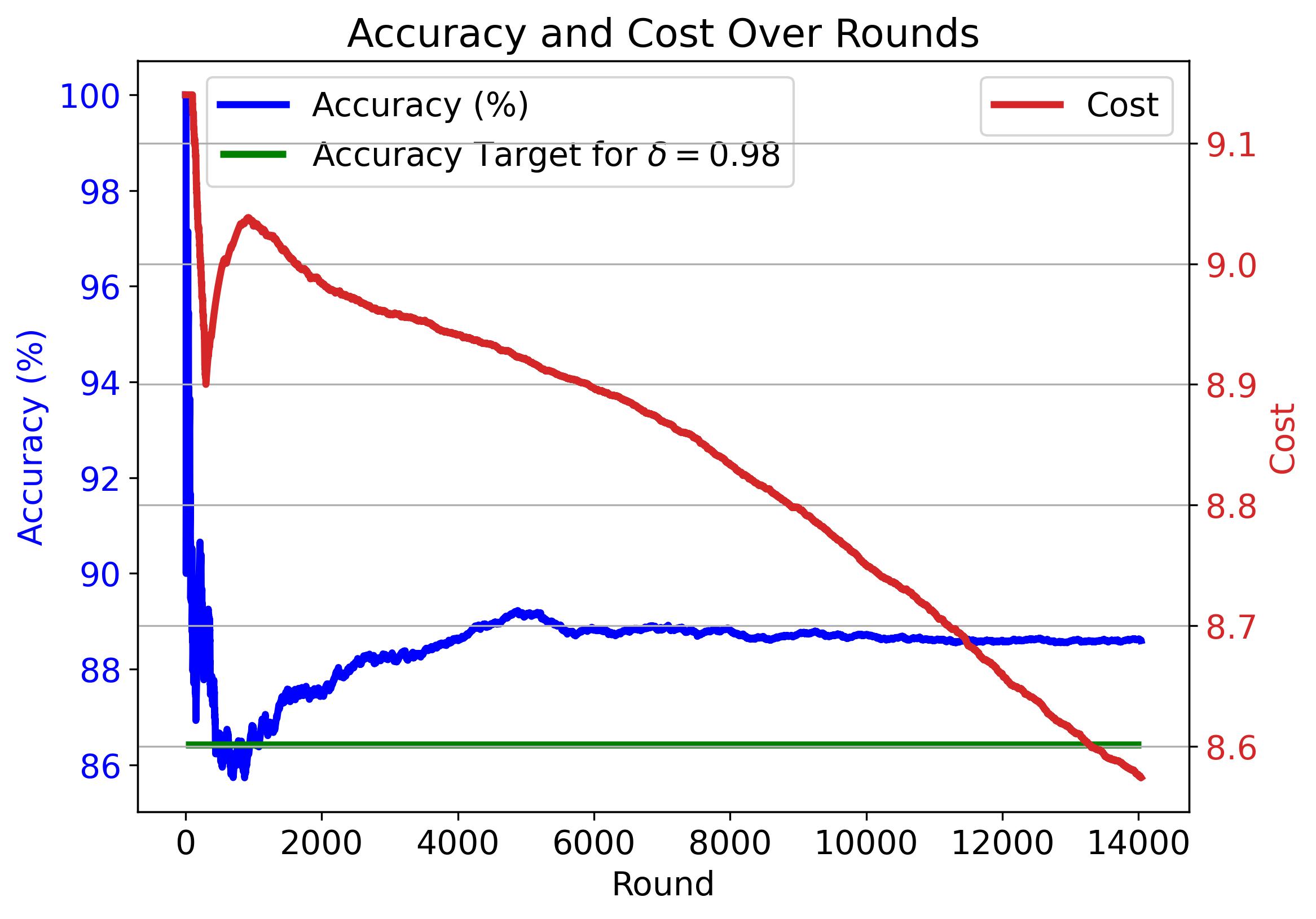
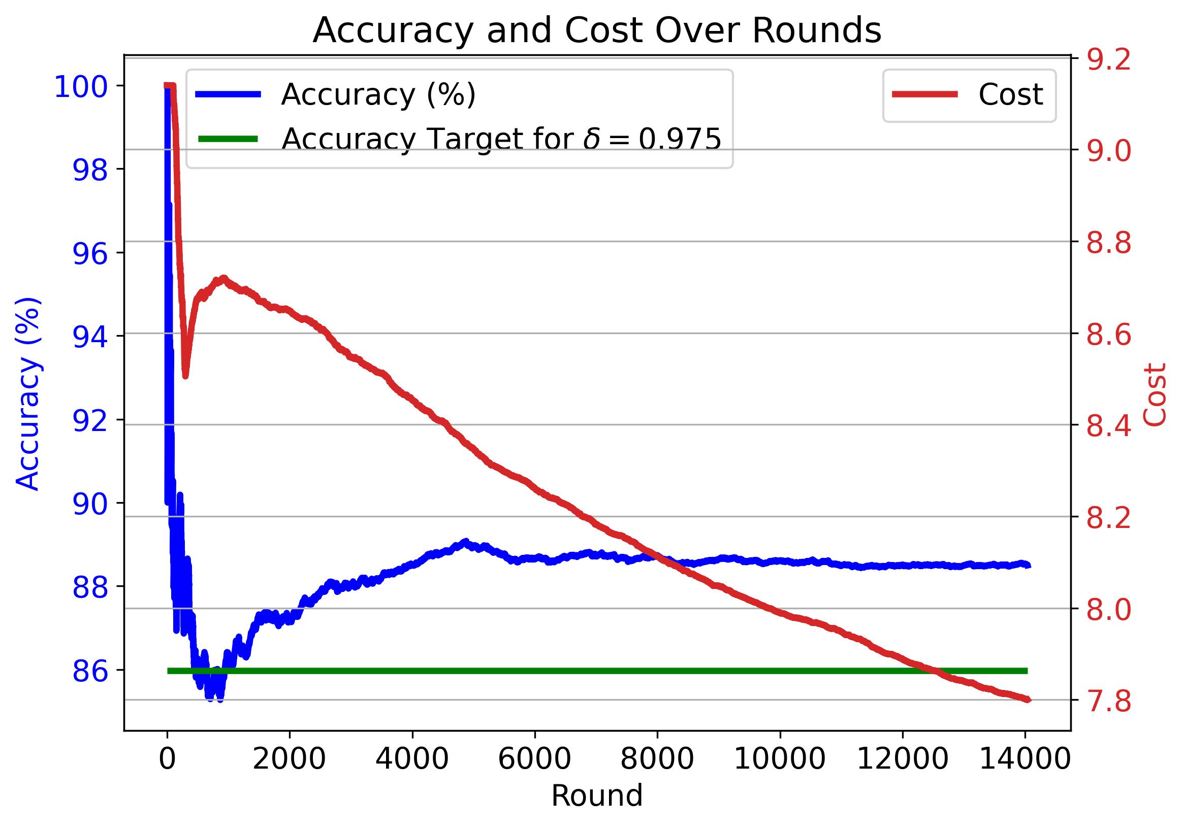
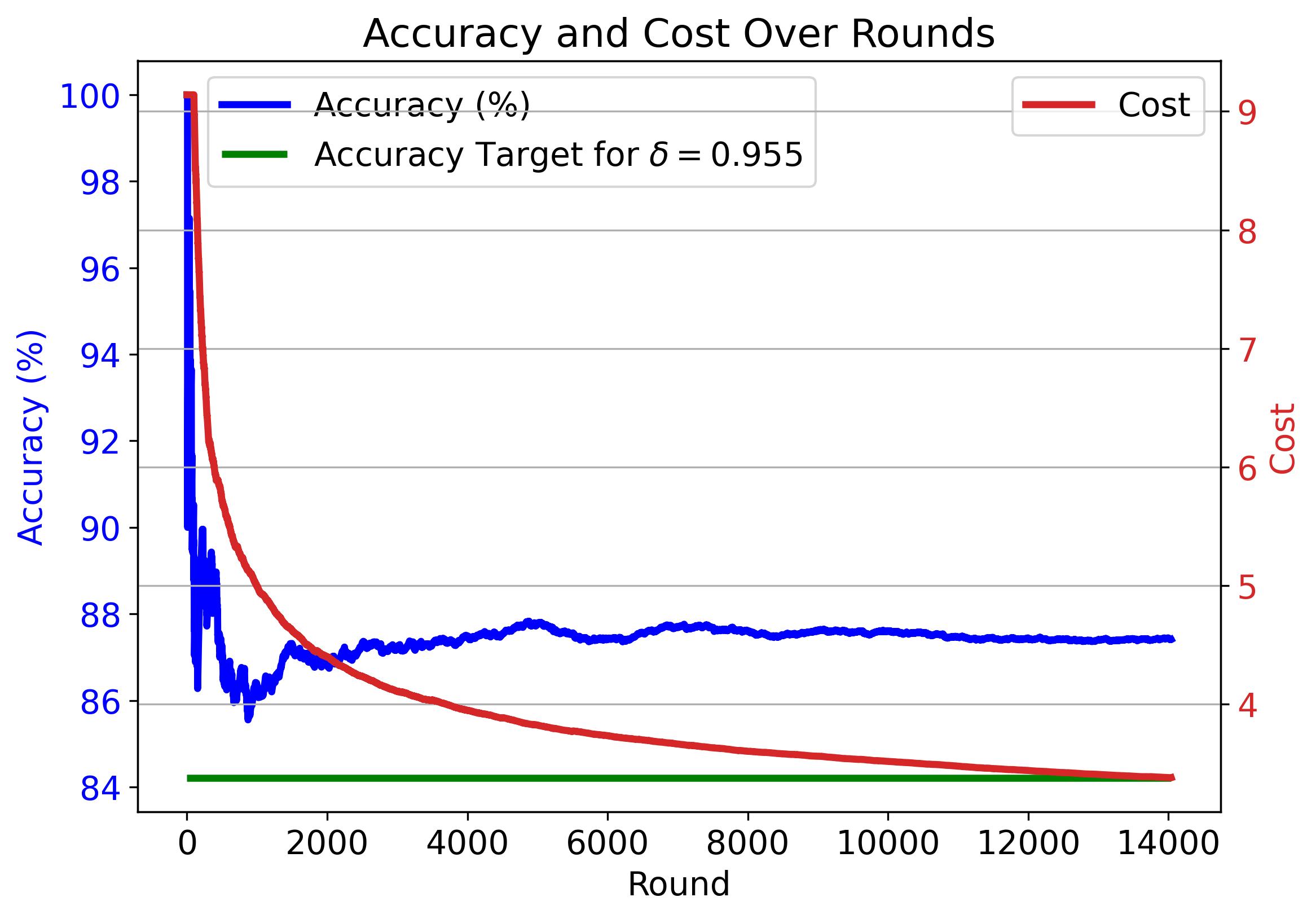
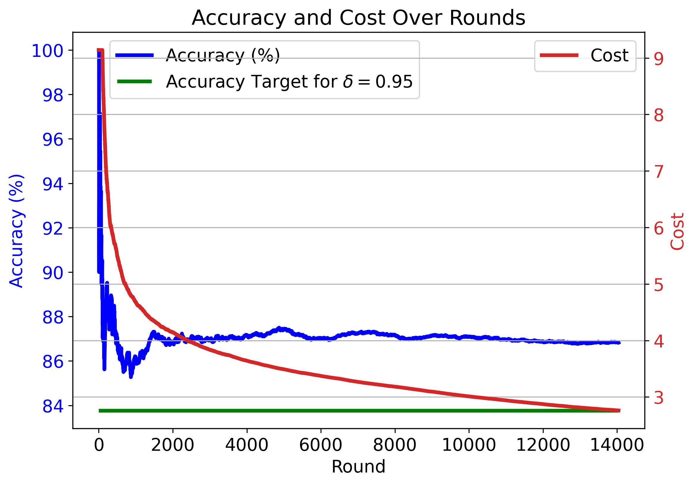
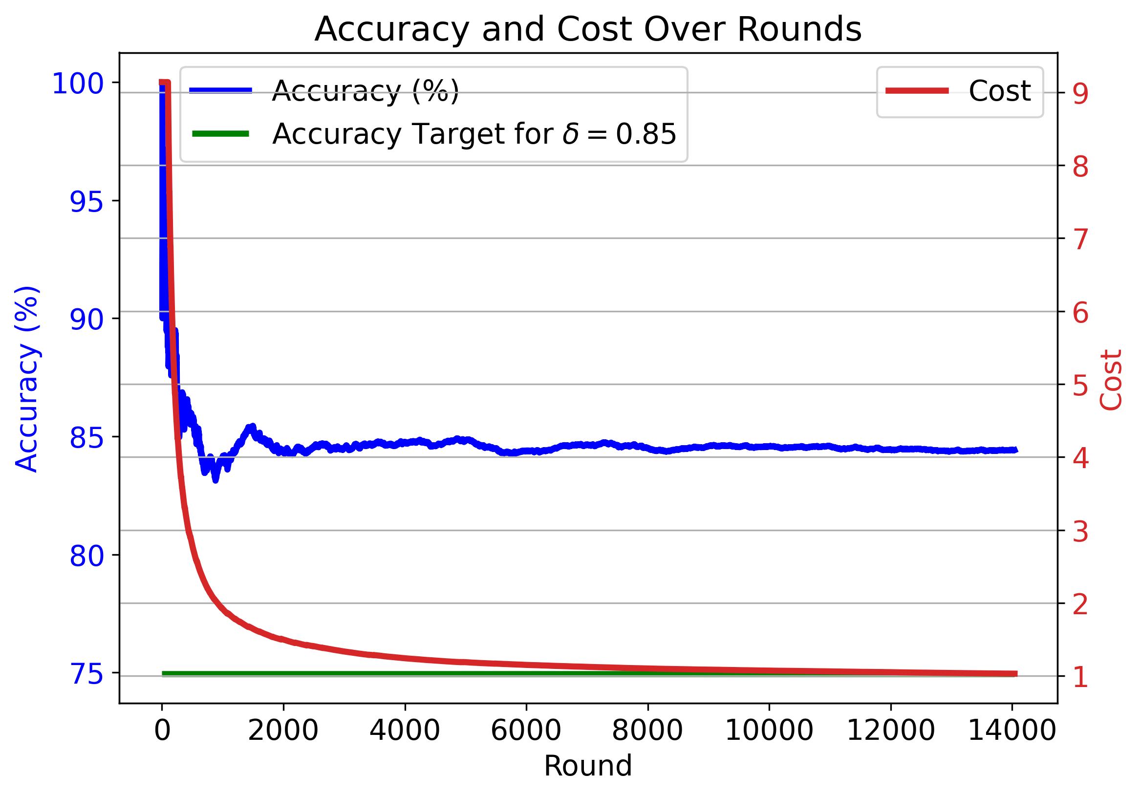
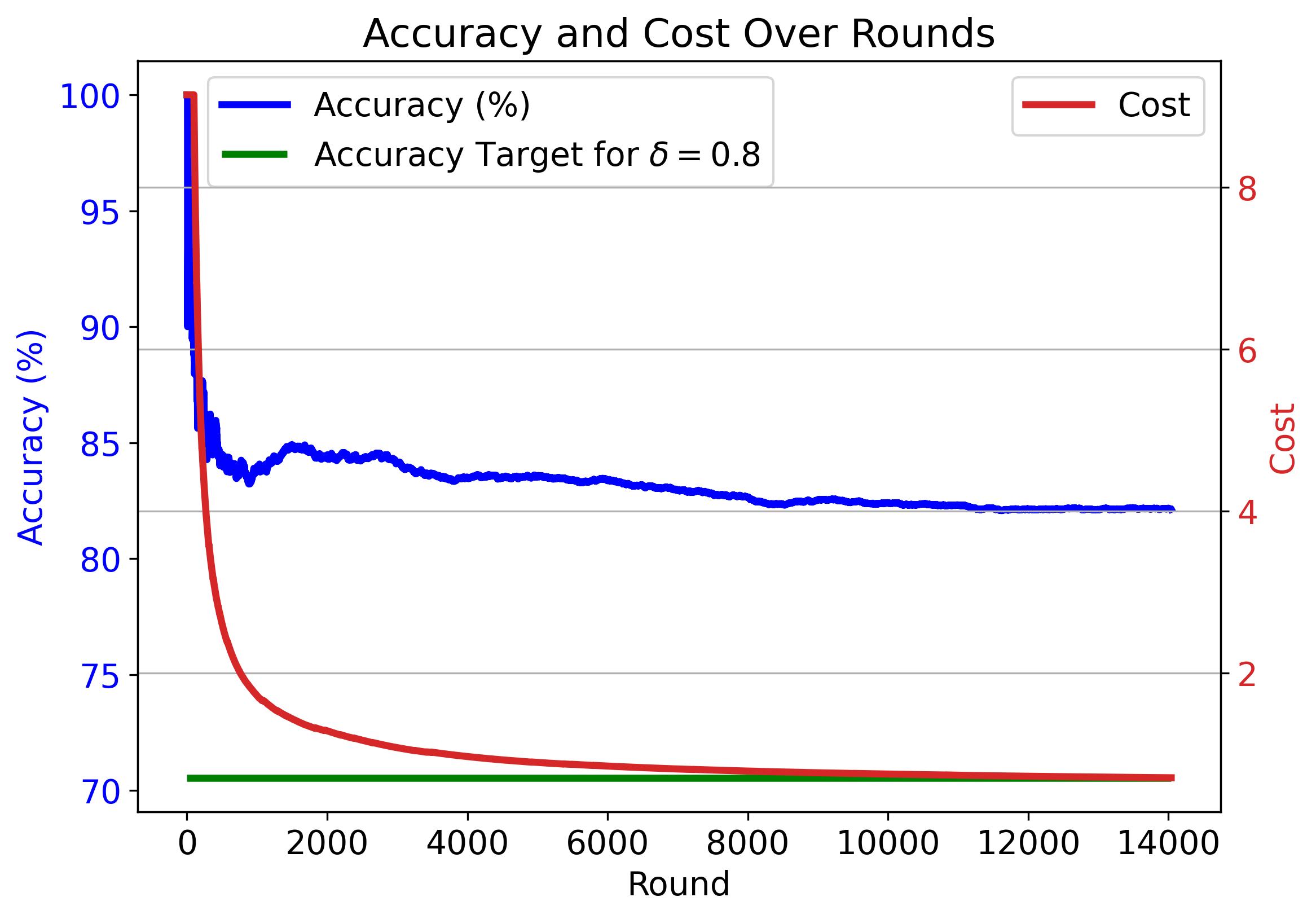
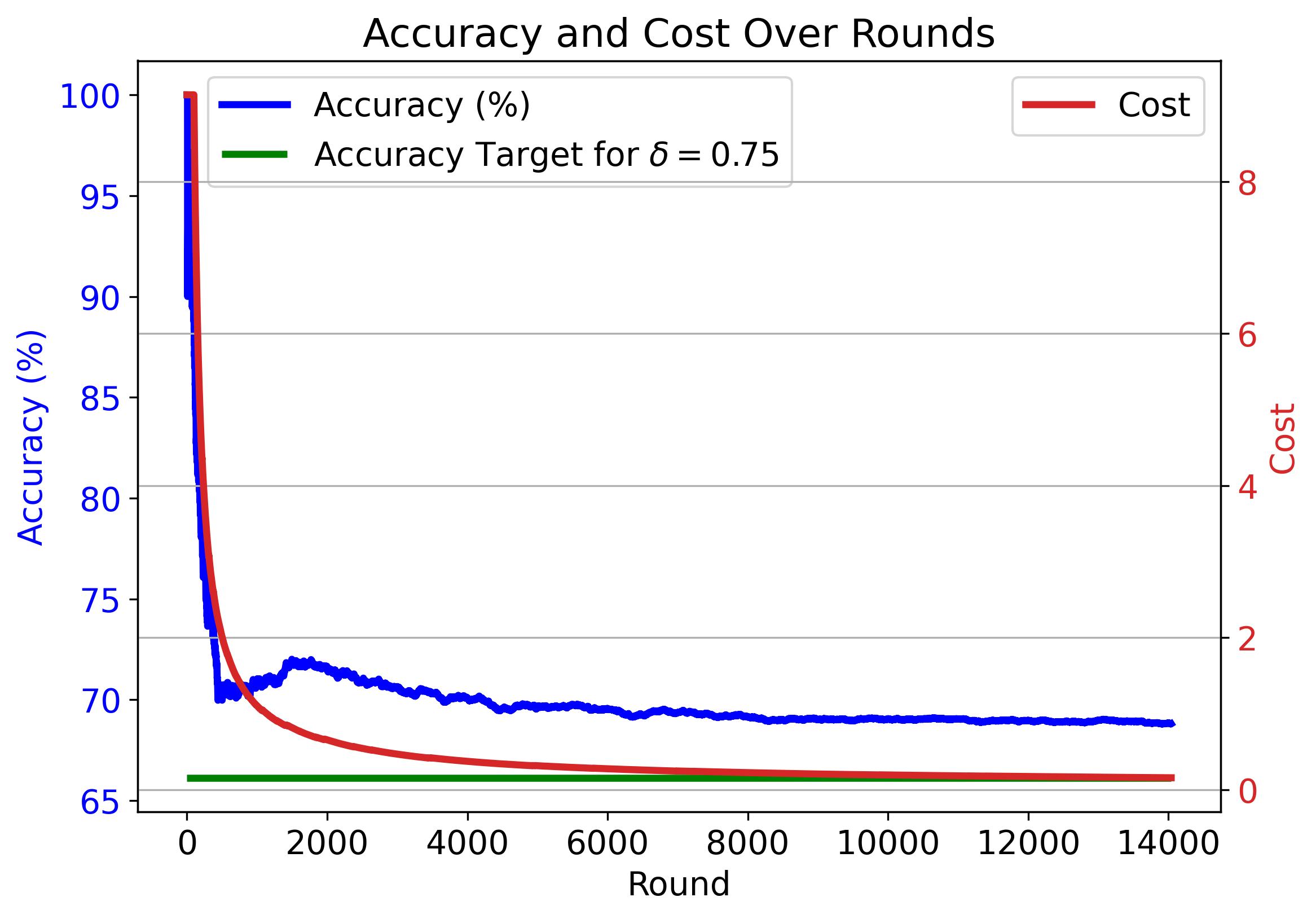
Figure 3: Cumulative average accuracy (blue) and cost (red) of CaMVo ($k_{\min}=1$) on the MMLU dataset across rounds for various $\delta$. The green line marks each $\delta$-specific target accuracy.

D.1 Additional Experimental Results

Figure 3 illustrates CaMVo’s cumulative average accuracy (blue) and cost (red) over rounds for $k_{\min}=1$ under different confidence thresholds $\delta$ to explore CaMVo’s learning dynamics for various $\delta$ values. The green line marks each $\delta$-specific target accuracy. In all cases, the algorithm begins by querying larger, more expensive ensembles to gather reliable performance estimates, then swiftly transitions to cheaper subsets once the lower-confidence bounds stabilize. This yields a steep decline in cost concurrent with accuracy settling at a value above the target line. A temporary dip in accuracy around round 1,000 appears consistently, reflecting a cluster of harder instances in our fixed data shuffle.

For high thresholds ($\delta=0.99$), CaMVo predominantly queries the full ensemble, producing an almost linear cost profile. At intermediate levels ($\delta=0.98,0.975$), cost initially falls but momentarily rises when accuracy dips below the target, prompting the algorithm to select slightly costlier subsets to regain the required confidence as the accuracy estimations of individual LLMs decrease. When $\delta<0.965$, the cost curve decreases monotonically and converges to a stable minimum, indicating rapid identification of the context-specific optimal subsets.

Finally, for low thresholds ($\delta=0.85,0.80$), observed accuracy significantly exceeds the target owing to the performance gaps among individual LLMs: no model has true accuracy between 70% and 80%, hence CaMVo’s conservative lower-bound estimates result in consistently higher realized accuracy. Overall, these results underscore CaMVo’s capacity to balance exploration and exploitation, quickly pinpoint cost-effective ensembles, and reliably meet user-specified accuracy requirements.

Similarly, Figure 5 examines CaMVo’s learning curves for various $\delta$ values with $k_{\min}=3$. As before, CaMVo starts by querying larger, costlier ensembles to estimate model performance, then quickly shifts to cheaper subsets once the lower-confidence bounds converge. For $\delta\geq 0.95$, the trajectories closely mirror those with $k_{\min}=1$. When $\delta\leq 0.90$, however, both accuracy and cost stabilize even more rapidly—reflecting convergence to the least-expensive three-LLM ensemble. This demonstrates that increasing $k_{\min}$ enhances stability by preventing undersized subsets from being chosen at the expense of a modest cost increase.

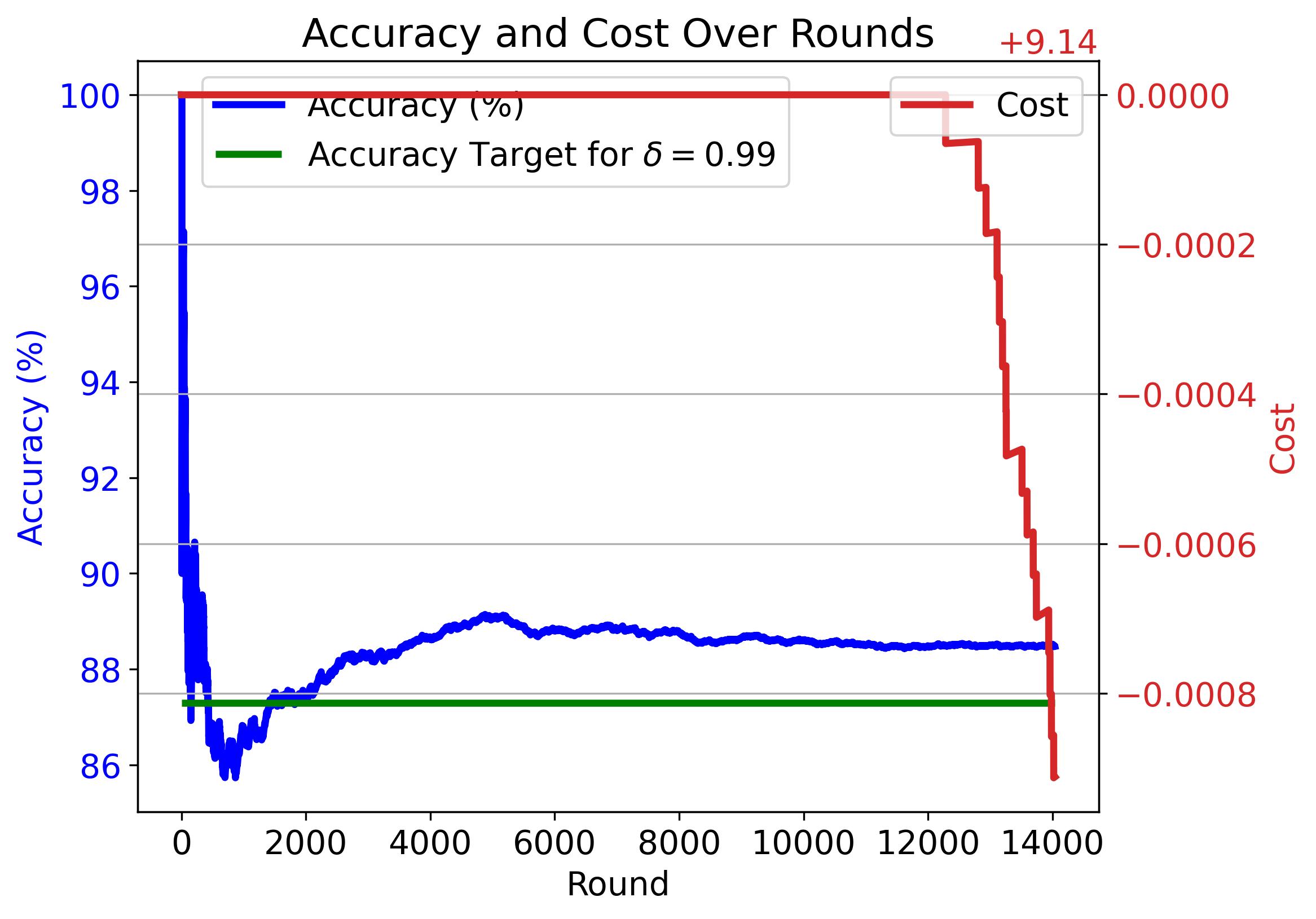
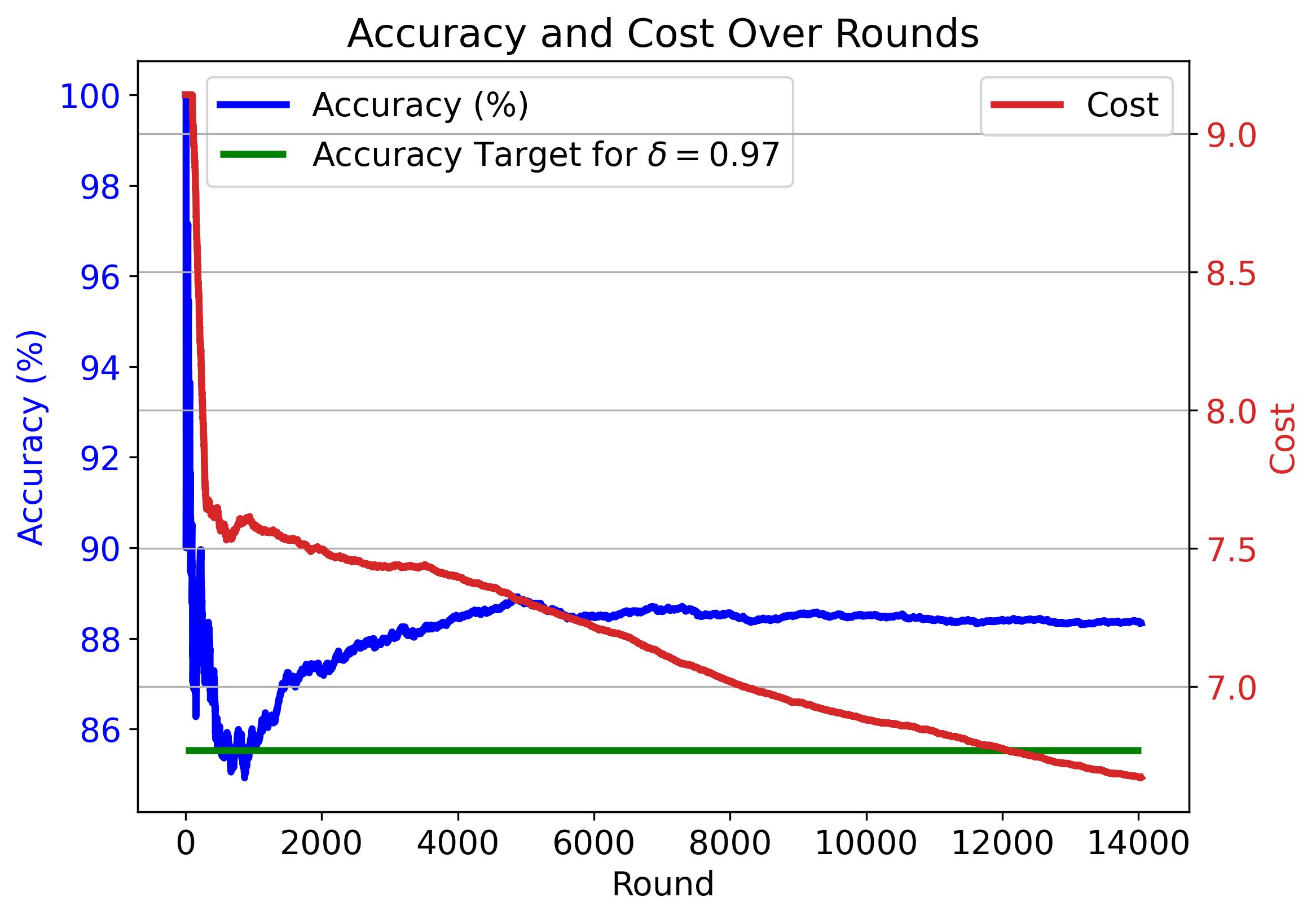
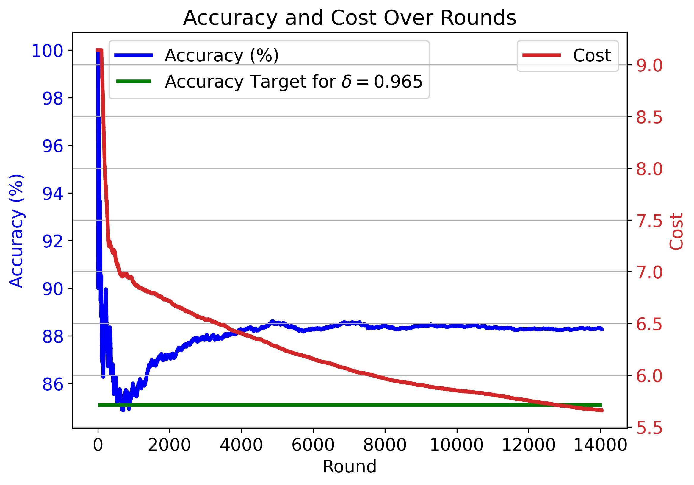
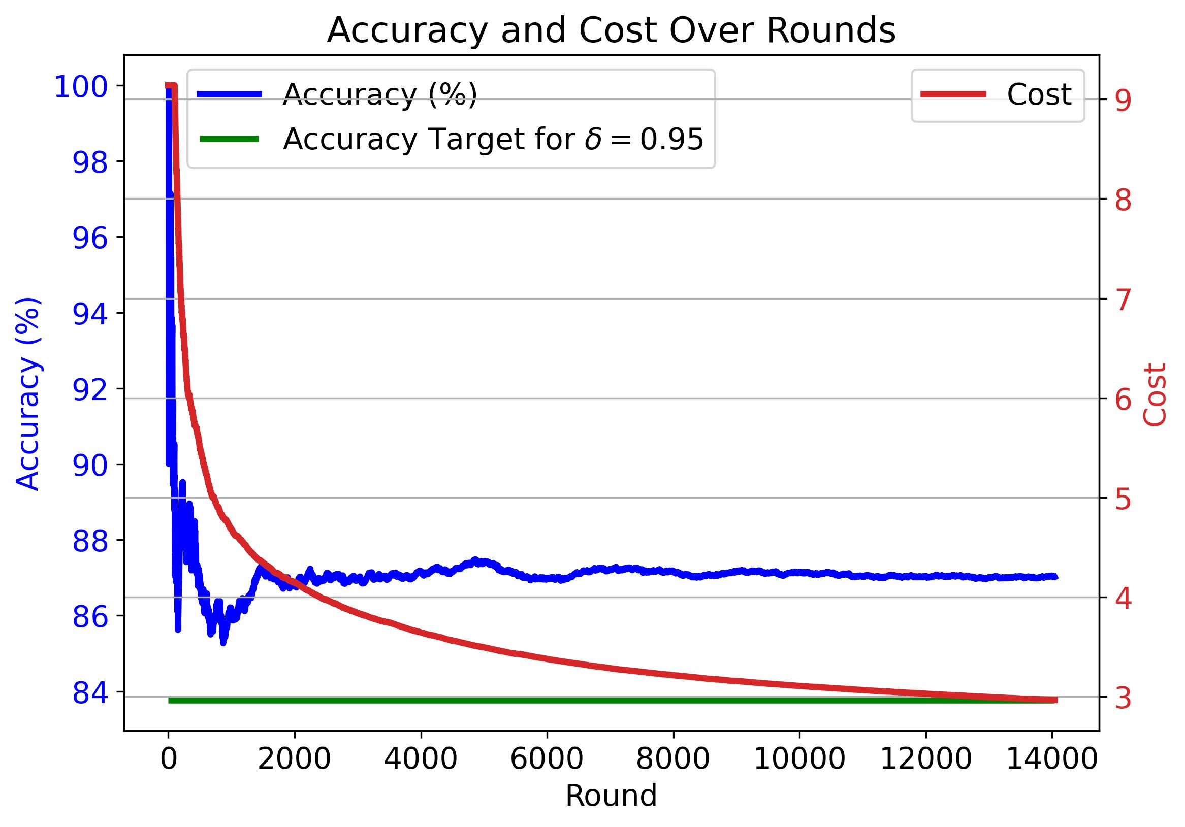
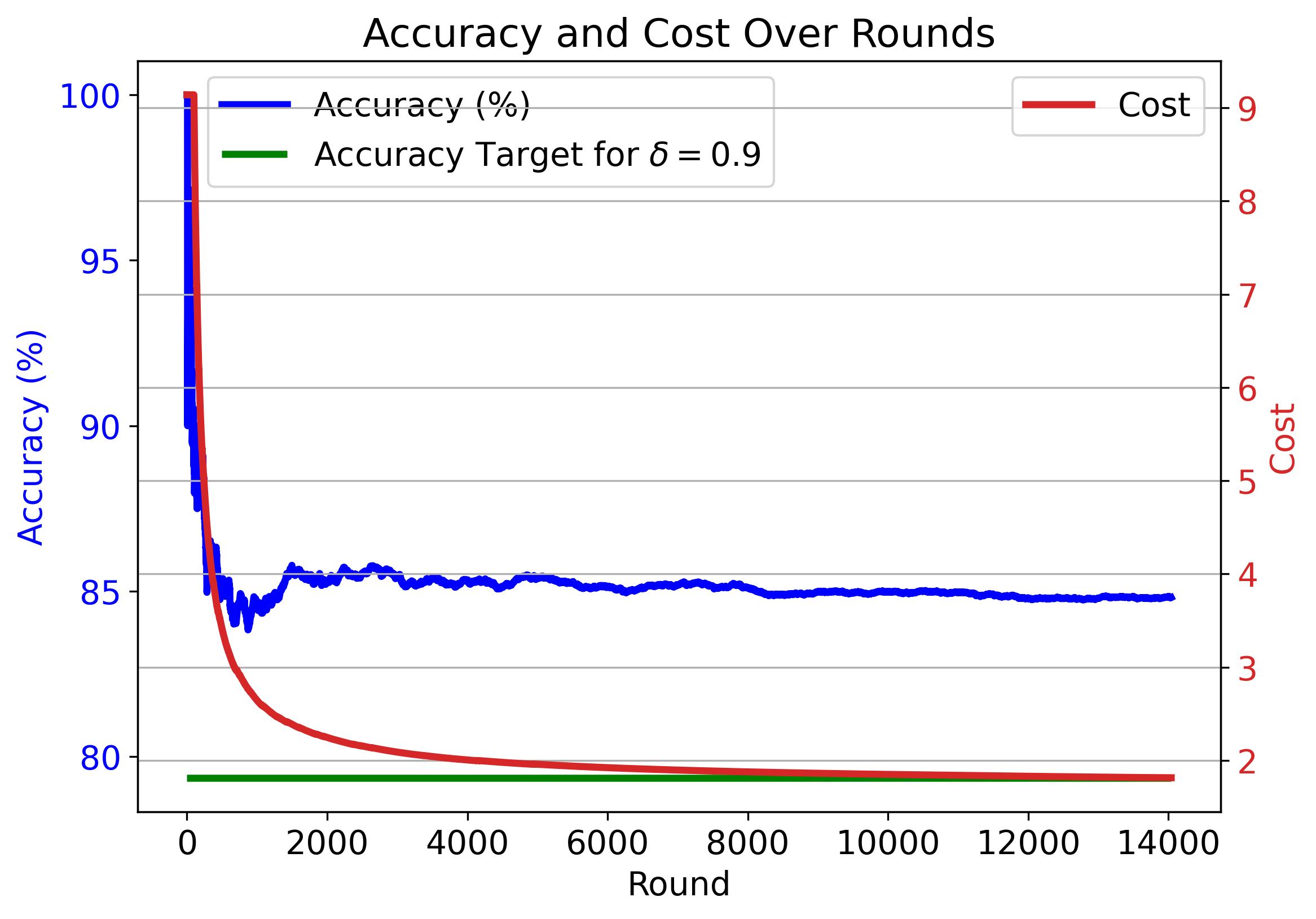
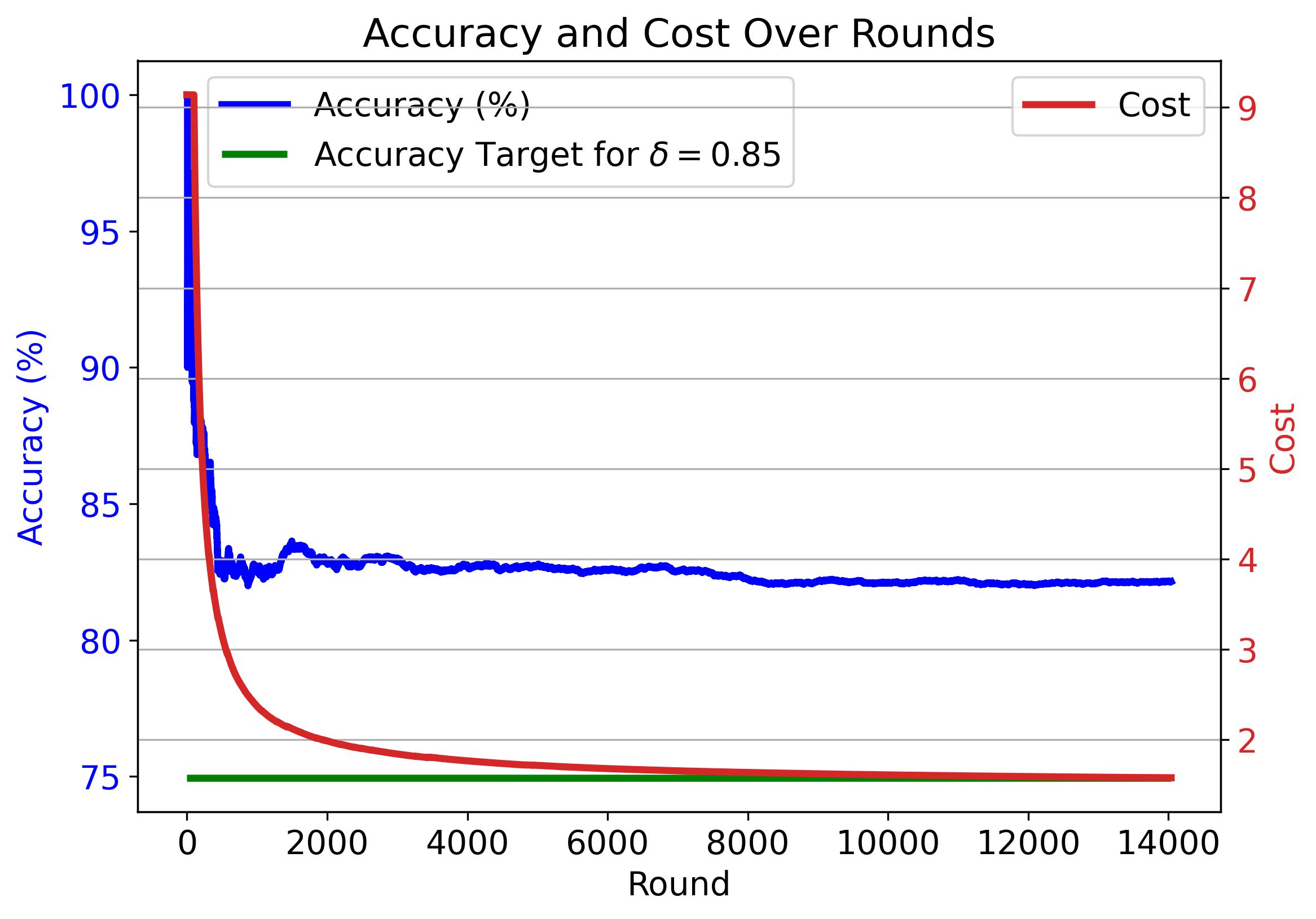
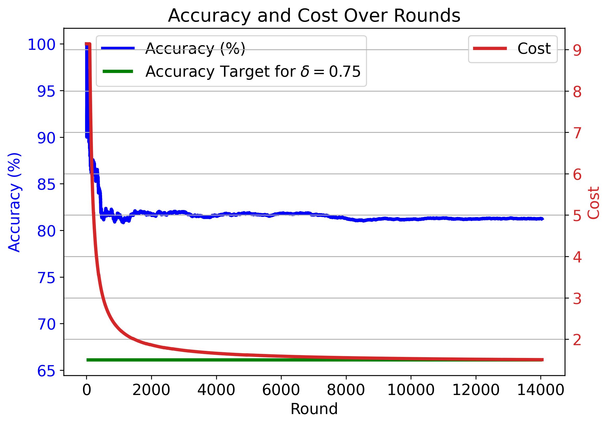
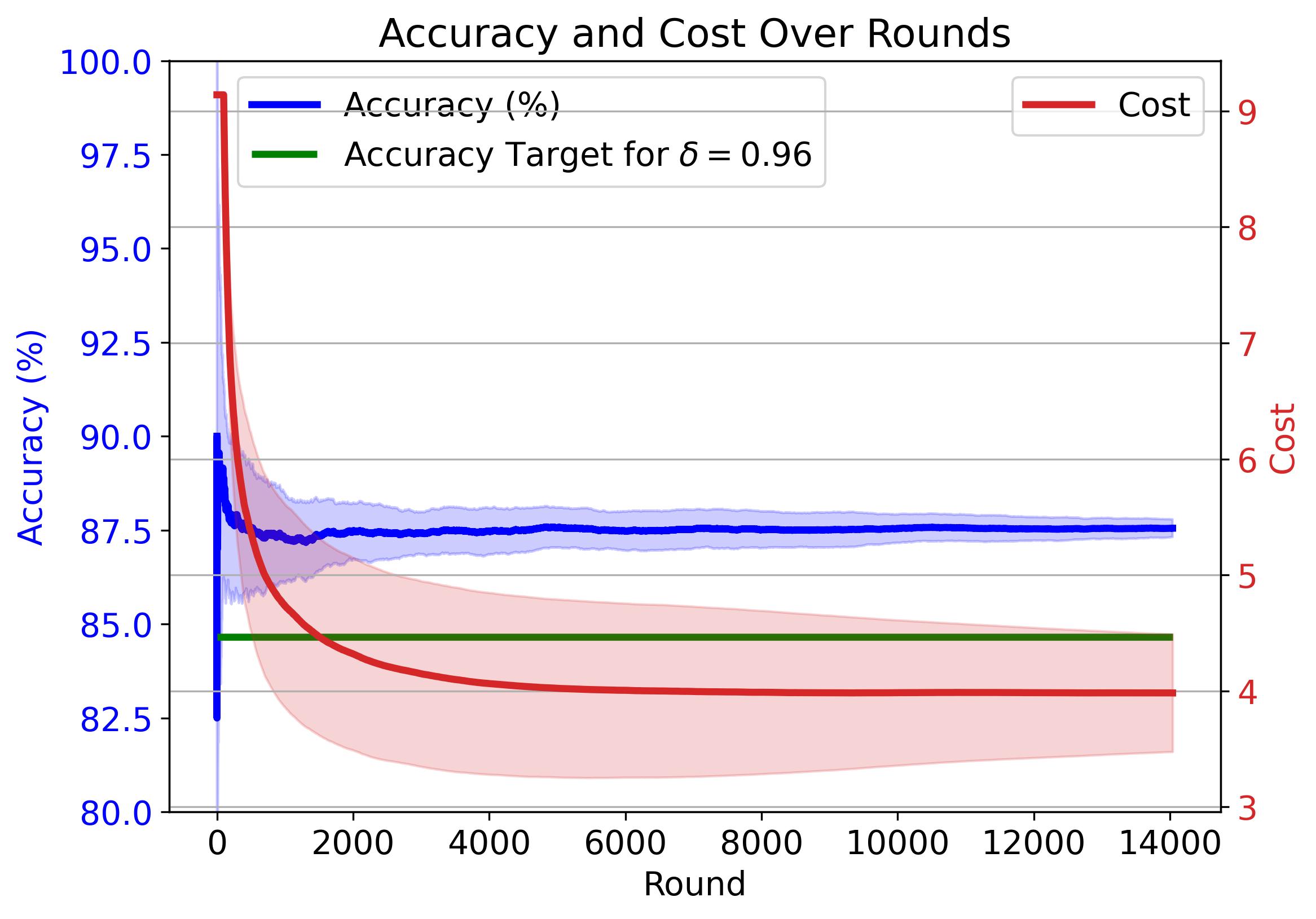
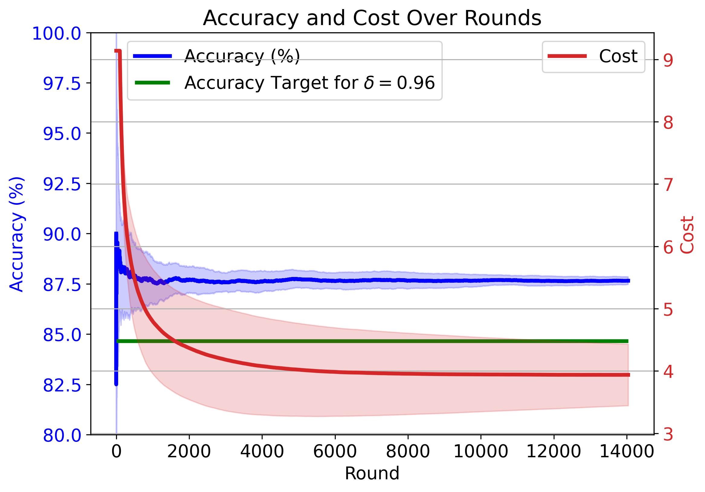
Figure 4: Cumulative average accuracy (blue) and cost (red) of CaMVo ($k_{\min}=3$) on the MMLU dataset across rounds for various $\delta$. The green line marks each $\delta$-specific target accuracy.

Figure 5: Mean (solid lines) and one-standard-deviation bands (shading) of CaMVo’s cumulative average accuracy (blue) and cost (red) over 20 random shuffles of MMLU when $\delta=0.96$ , $k_{\min}=1$ (Left); and $\delta=0.96$ , $k_{\min}=1$ (Right). The green line indicates the accuracy target of $84.65\%$ for $\delta=0.96$.

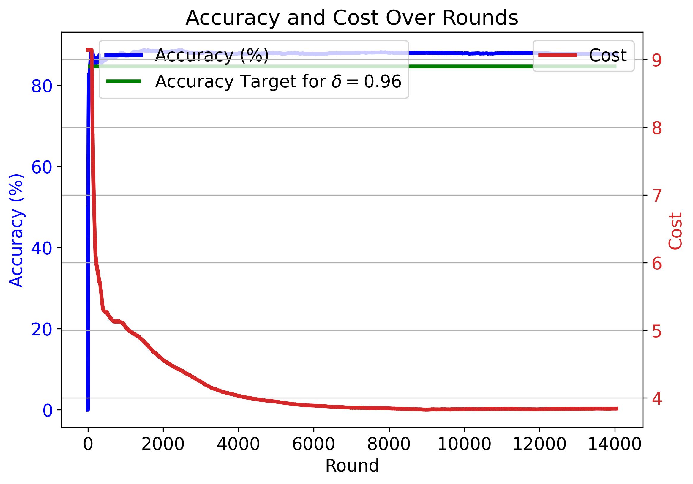
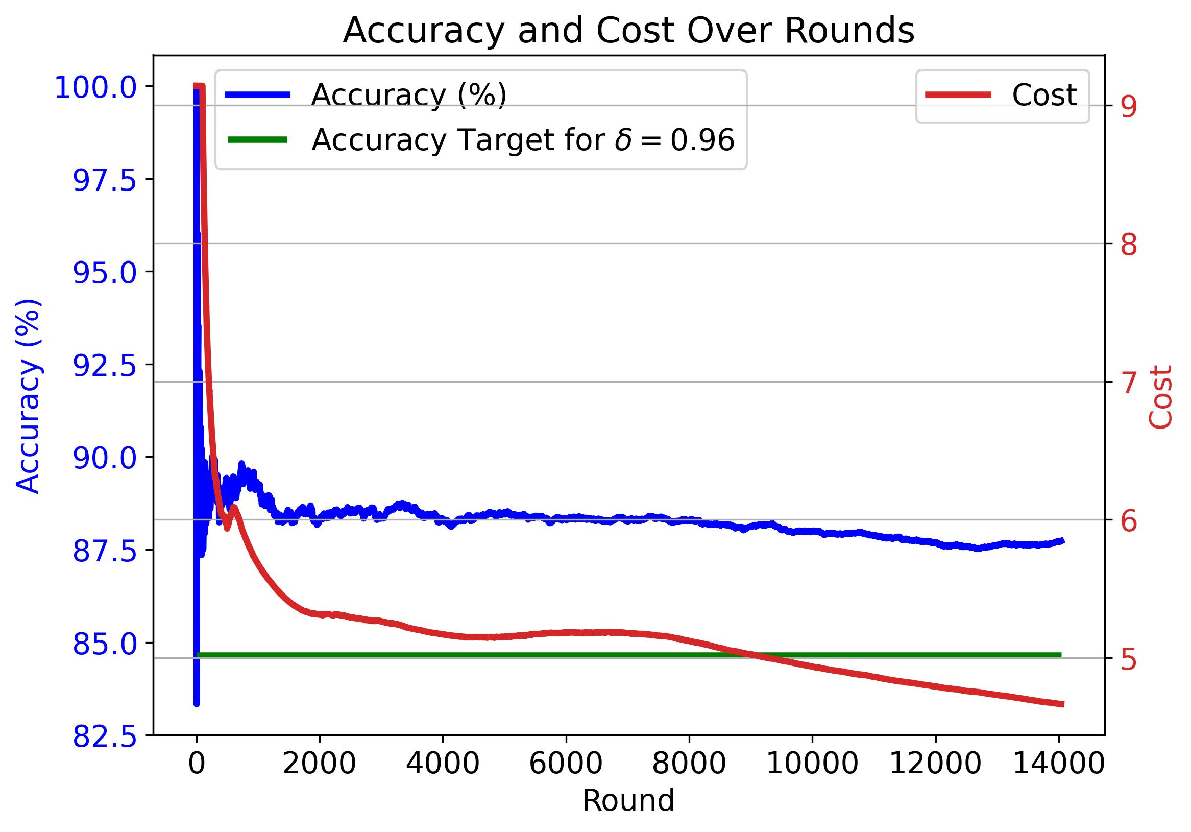
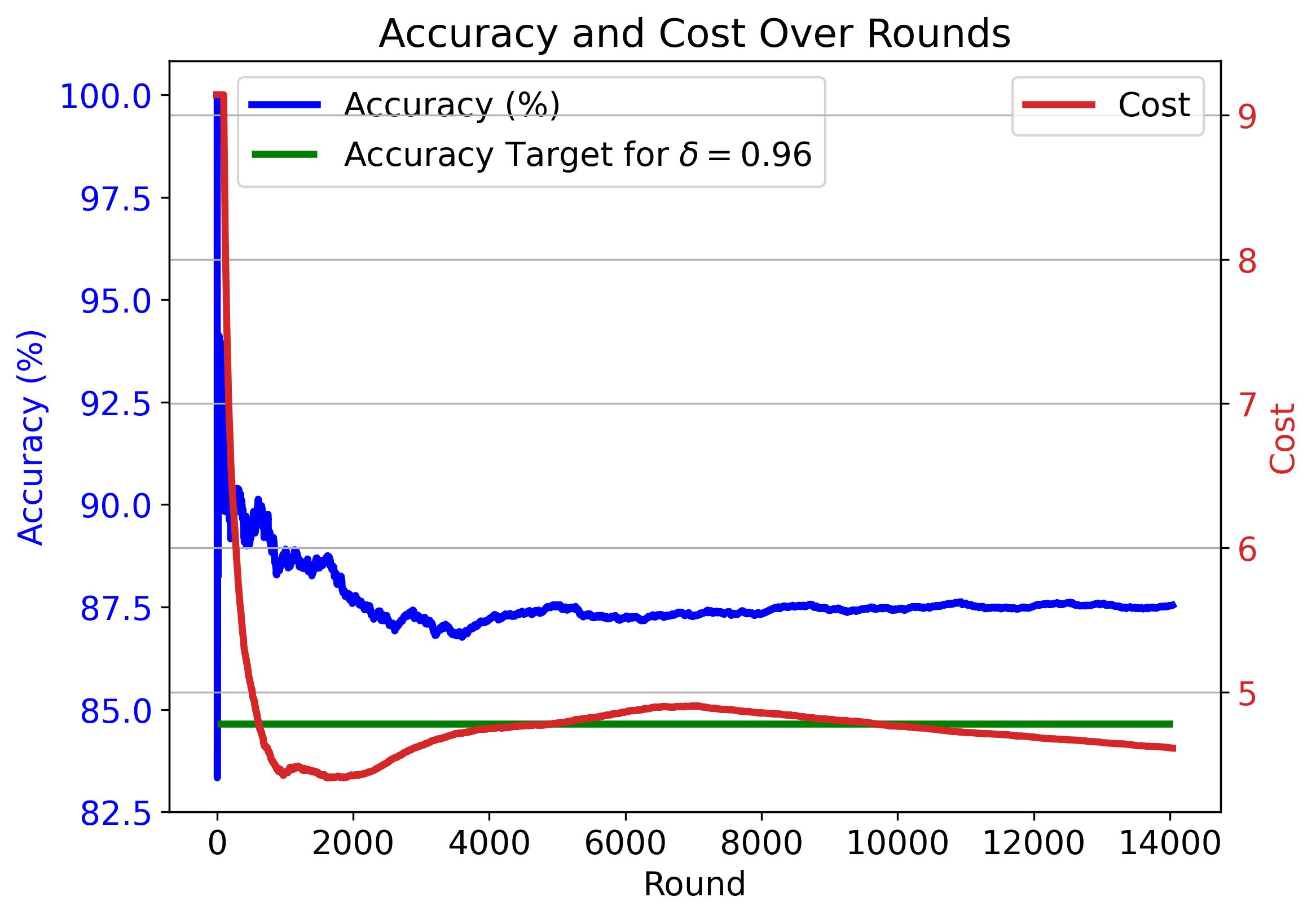
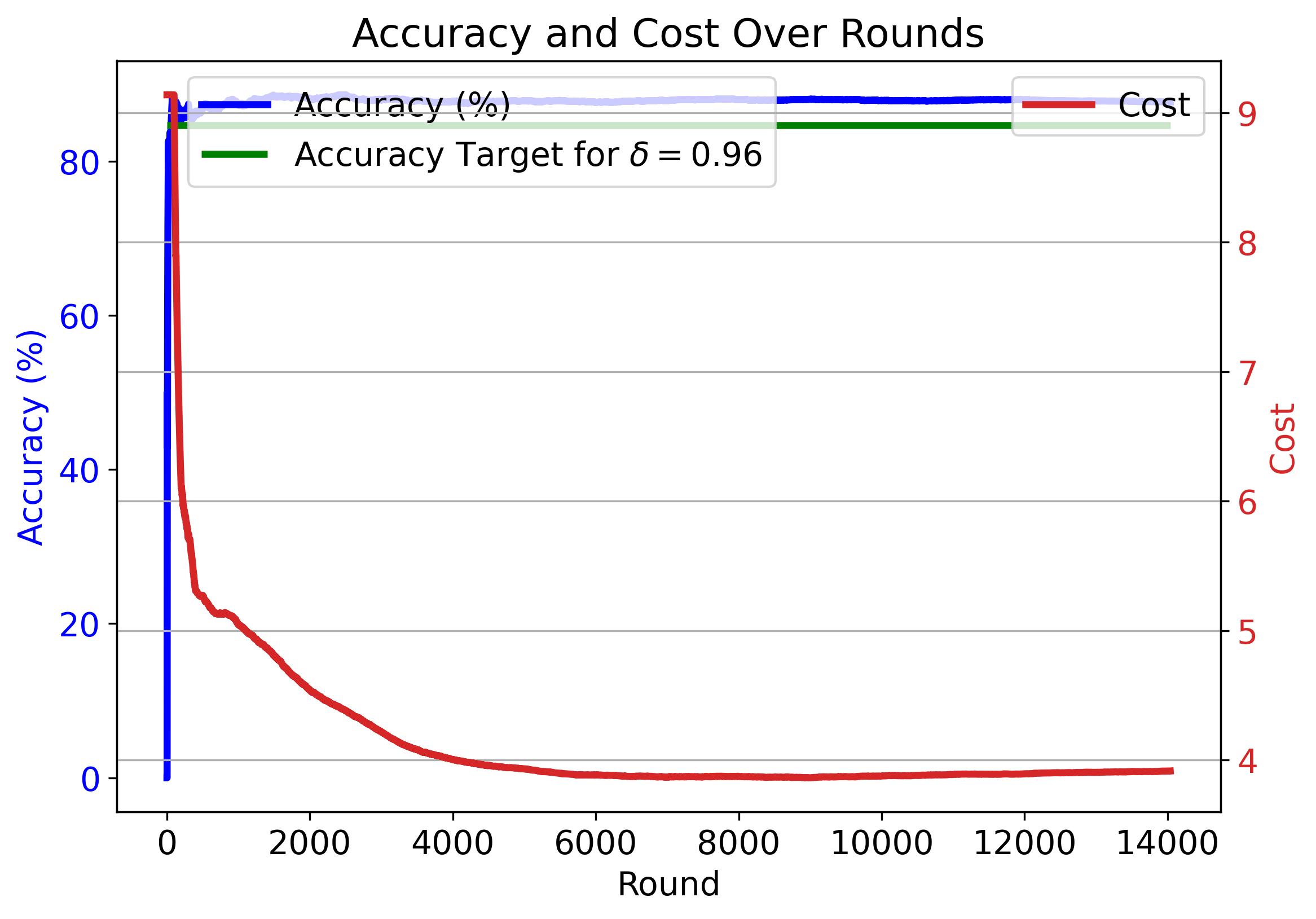
Figure 6: Cumulative average accuracy (blue) and cost (red) of CaMVo with $\delta=0.96$, $k_{\min}=1$ under nine different permutations of the dataset. The green line marks each $\delta$-specific target accuracy.

Figure 7: Cumulative average accuracy (blue) and cost (red) of CaMVo with $\delta=0.96$, $k_{\min}=3$ under nine different permutations of the dataset. The green line marks each $\delta$-specific target accuracy.

Further, to evaluate CaMVo’s robustness to input ordering, Figure 5 shows the mean cumulative average accuracy and cost trajectories (solid lines) averaged over 20 random shuffles of the MMLU dataset for $\delta=0.96$, $k_{\min}=1$ (Left); and for $\delta=0.96$, $k_{\min}=3$ (Right). Shaded bands denote one standard deviation. Although the accuracy band is initially wide due to the exploration of CaMVo, and also different mixes of easy and hard examples across the shuffles; it contracts rapidly, underscoring CaMVo’s consistent attainment of the target accuracy across permutations. The cost band also narrows over time, illustrating stable convergence to low-cost ensembles. Notably, the accuracy band remains much tighter than the cost band, since CaMVo targets above the accuracy threshold but does not optimize for a fixed cost. Comparing $k_{\min}=1$ and $k_{\min}=3$, it can be seen that both the cost and accuracy bands are similar.

To evaluate CaMVo’s robustness to input ordering in more detail, Figure 7 overlays the mean cumulative average accuracy and cost plots of nine individual runs from these permutations. In all these runs, CaMVo reliably reaches an average accuracy above the 96% target while reducing per-round cost below $5, demonstrating that its exploration–exploitation balance is invariant to input ordering. Figure 7 presents the corresponding results for the $k_{\min}=3$ setting, confirming similar robustness to input permutations.

Appendix E Supplementary Details for Experiments on the IMDB Movie Reviews Dataset

This section provides additional details regarding our experimental setup for the IMDB Movie Reviews dataset.

First, to improve computational efficiency, we again approximate the confidence score $\delta_{\mathcal{A}}(\bm{L},\bm{\omega})$ using the cumulative distribution function (CDF) of the Beta distribution rather than the closed-form expression in Lemma 2.1:

$$\delta_{\mathcal{A}}(\bm{L},\bm{\omega})\approx 1-F_{\text{Beta}}\left(0.5;\,W_{L,\mathcal{A}},\,W_{\mathcal{A}}-W_{L,\mathcal{A}}\right),$$

where $F_{\text{Beta}}(x;\alpha,\beta)$ is the CDF of a $\text{Beta}(\alpha,\beta)$ distribution, $W_{L,\mathcal{A}}=\sum_{i\in\mathcal{A}}\omega_{i}\cdot L_{i}$, and $W_{\mathcal{A}}=\sum_{i\in\mathcal{A}}\omega_{i}$.

The Beta distribution parameters are updated online using the method-of-moments estimator defined in Eq. (21), with a regularization term $\epsilon=10^{-6}$.

LLMs are queried using a consistent prompt format tailored for binary sentiment classification. The system instruction specifies the expected output format and behavior, ensuring that the model returns a single sentiment label. The standard query format is shown below:

For LLMs that do not support separate system and user messages (e.g., via a chat API), the instruction is prepended directly to the user input.

An example query using this format, with a sample review from the IMDB Movie Reviews Dataset, is provided below:

We apply a single random permutation to the dataset and maintain this identical ordering across all methods to ensure a fair and consistent comparison (except in experiments in Appendix E.1 where we analyze the sensitivity of CaMVo to dataset ordering).

E.1 Additional Experimental Results

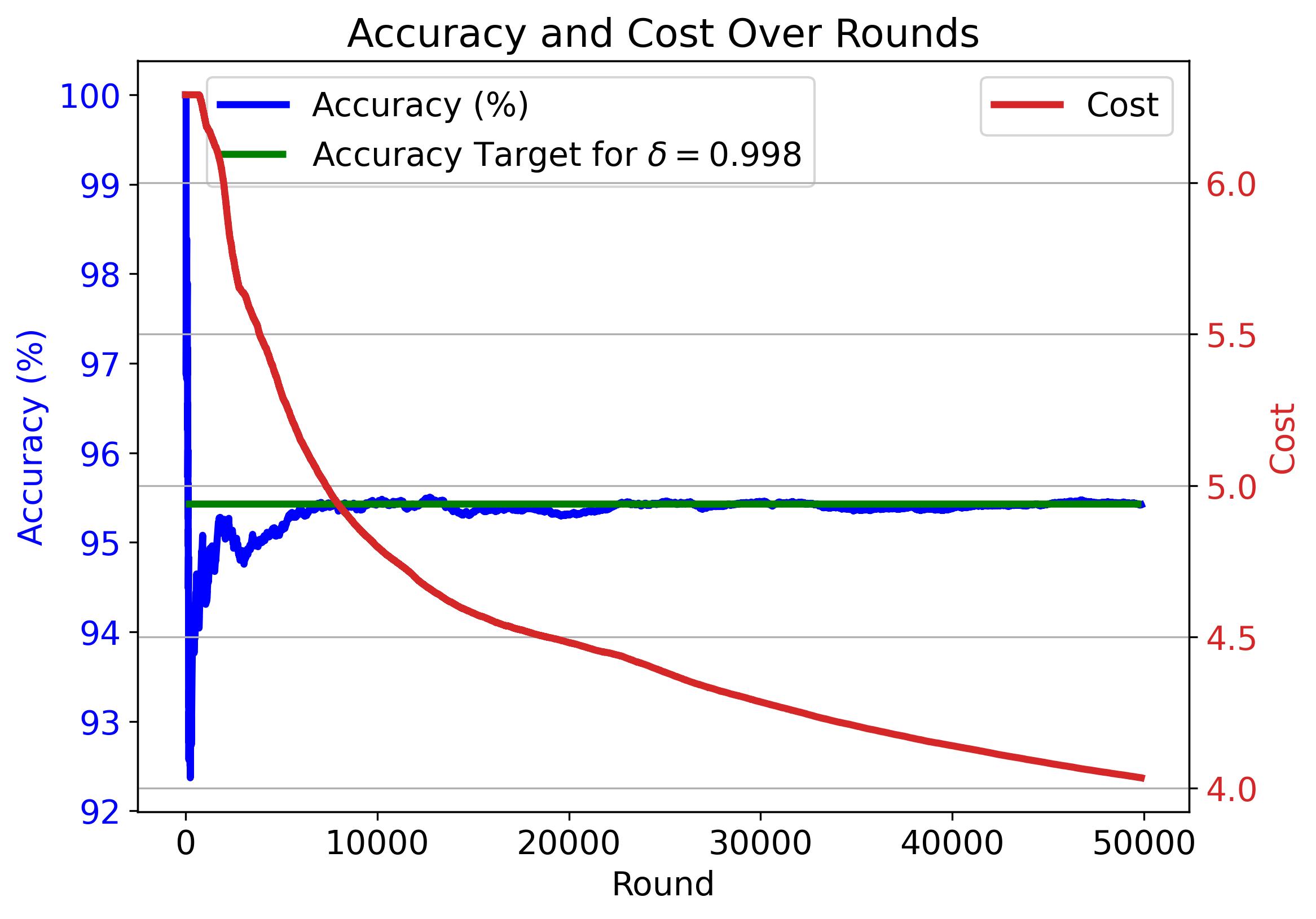
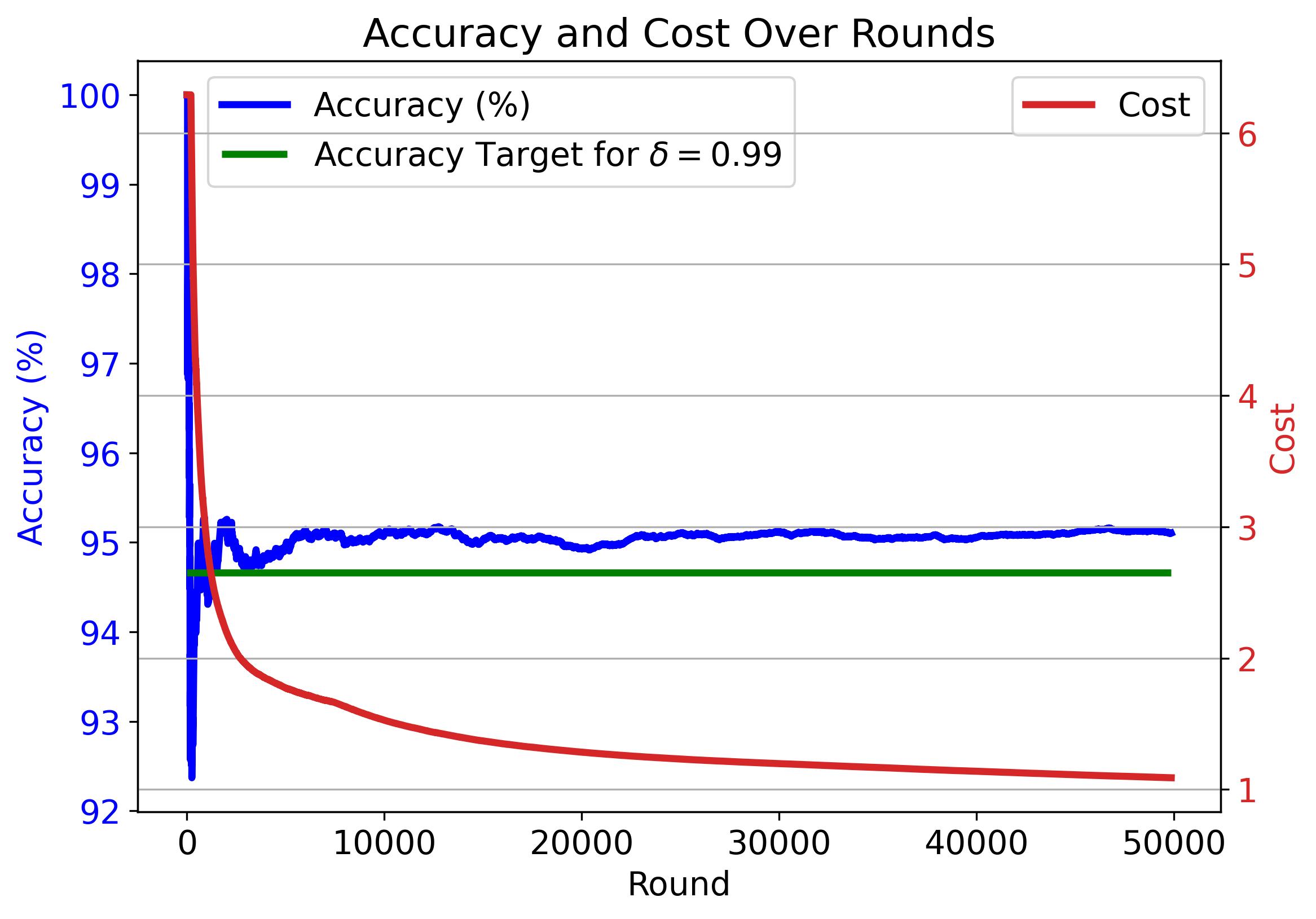
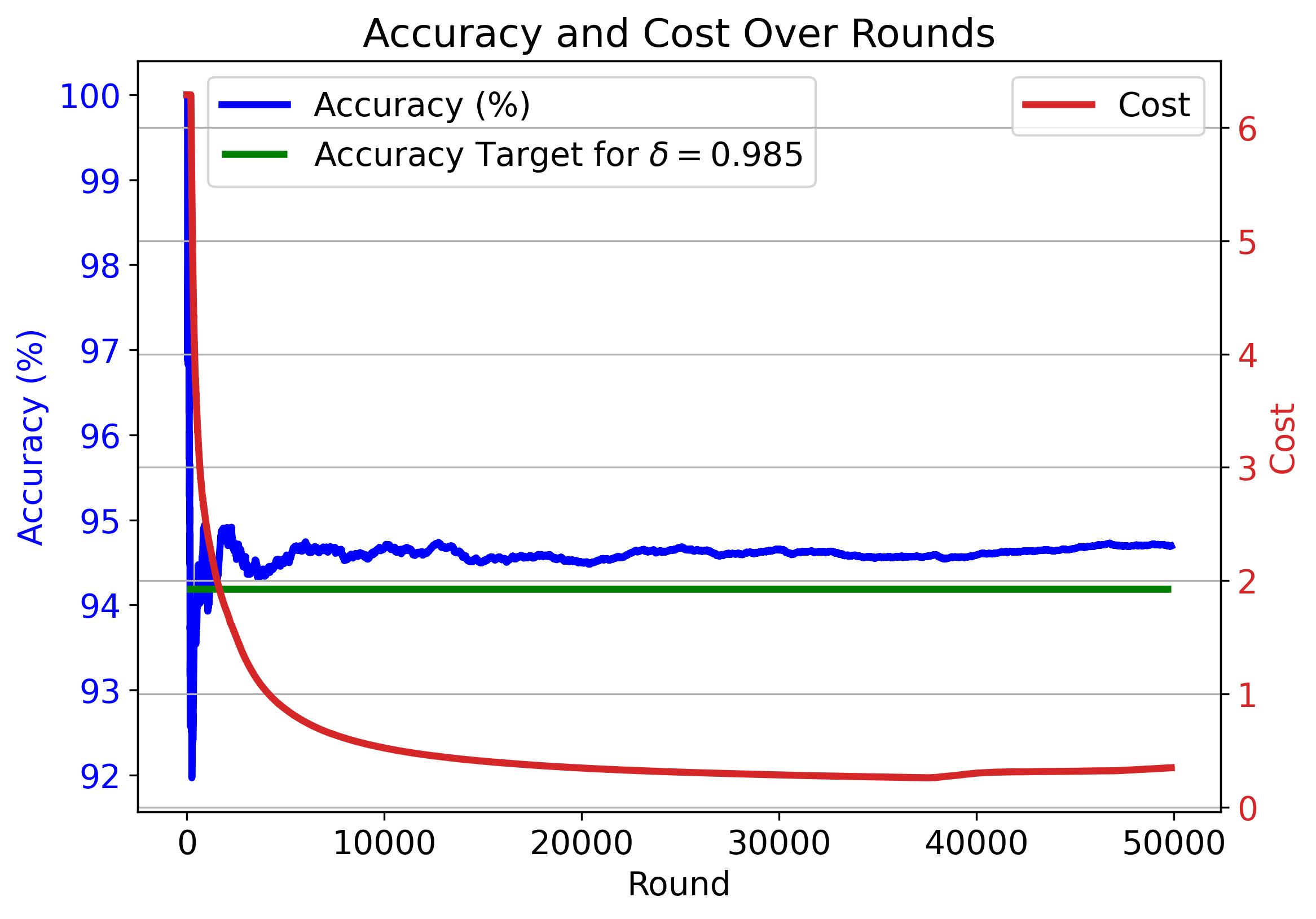
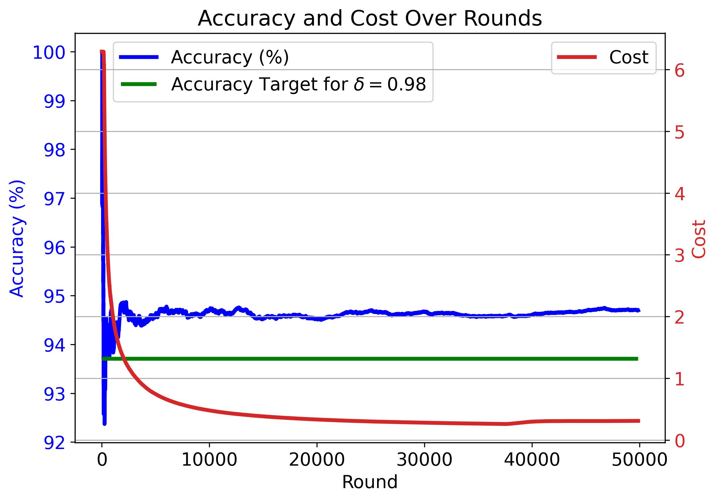
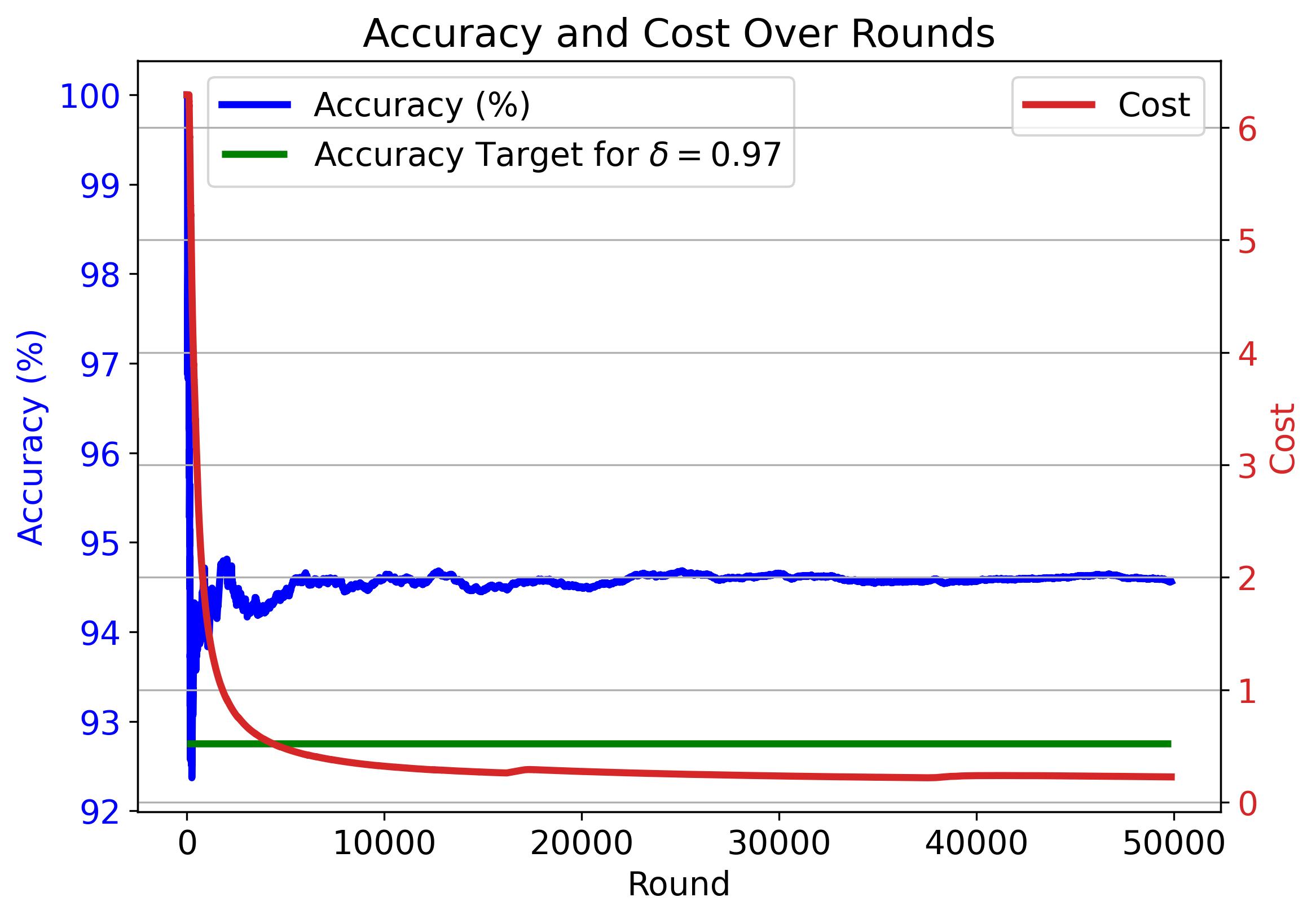
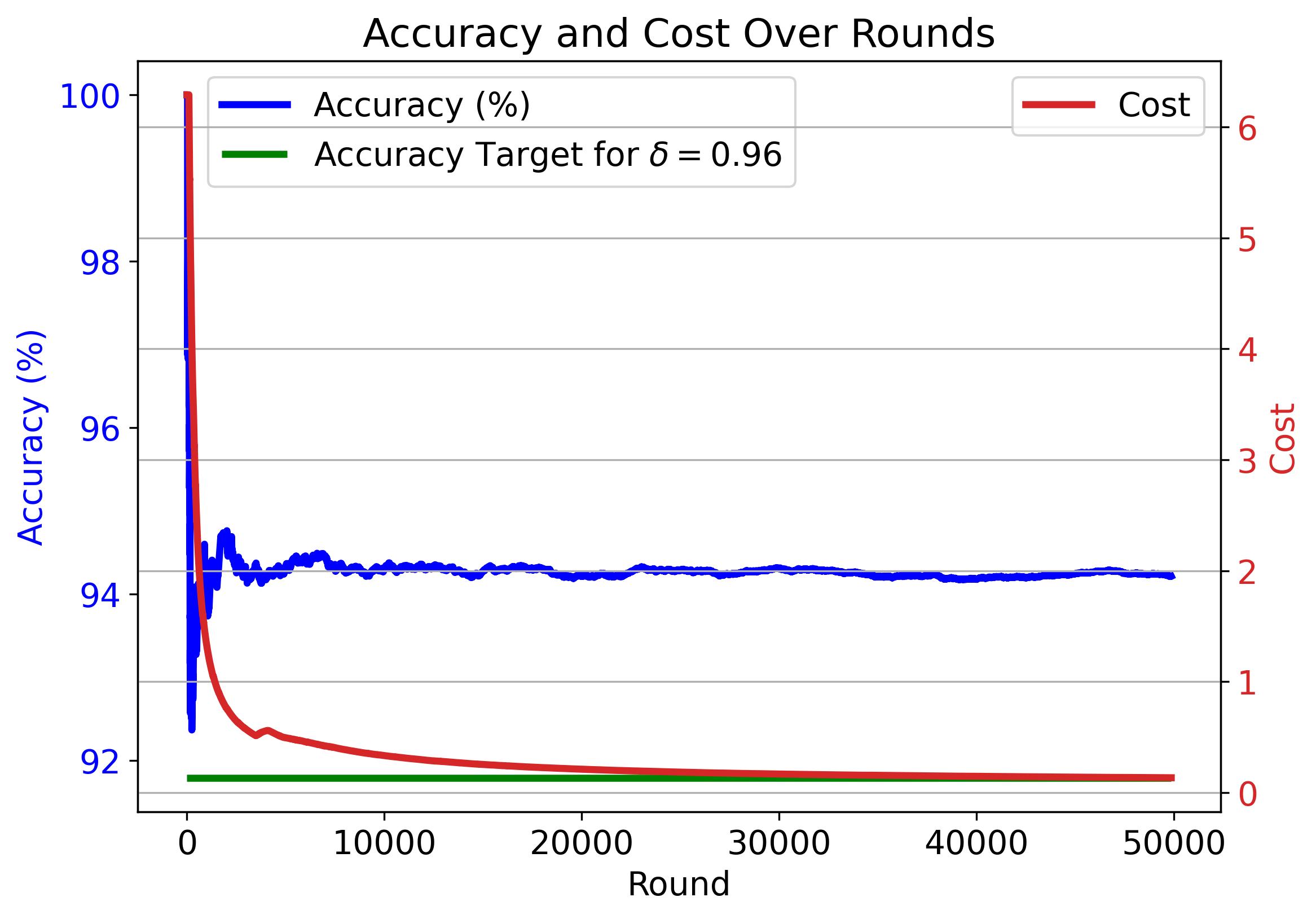
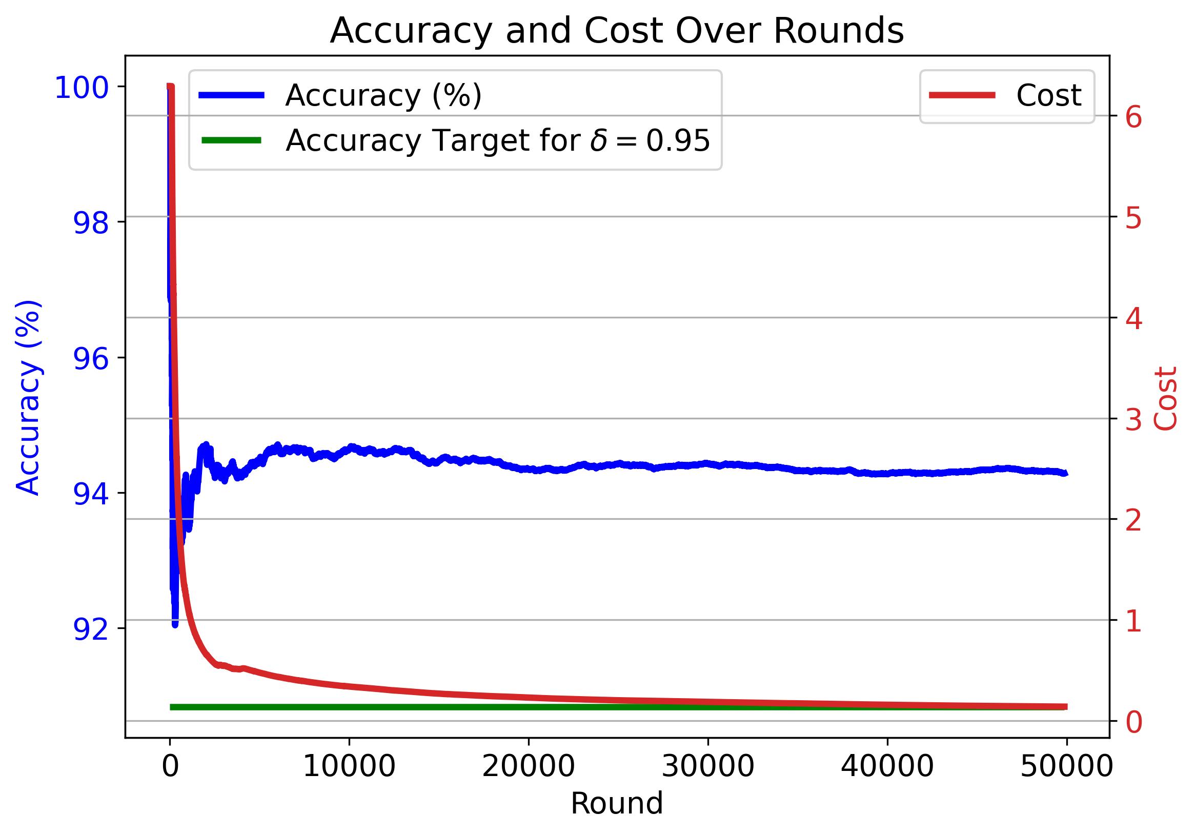
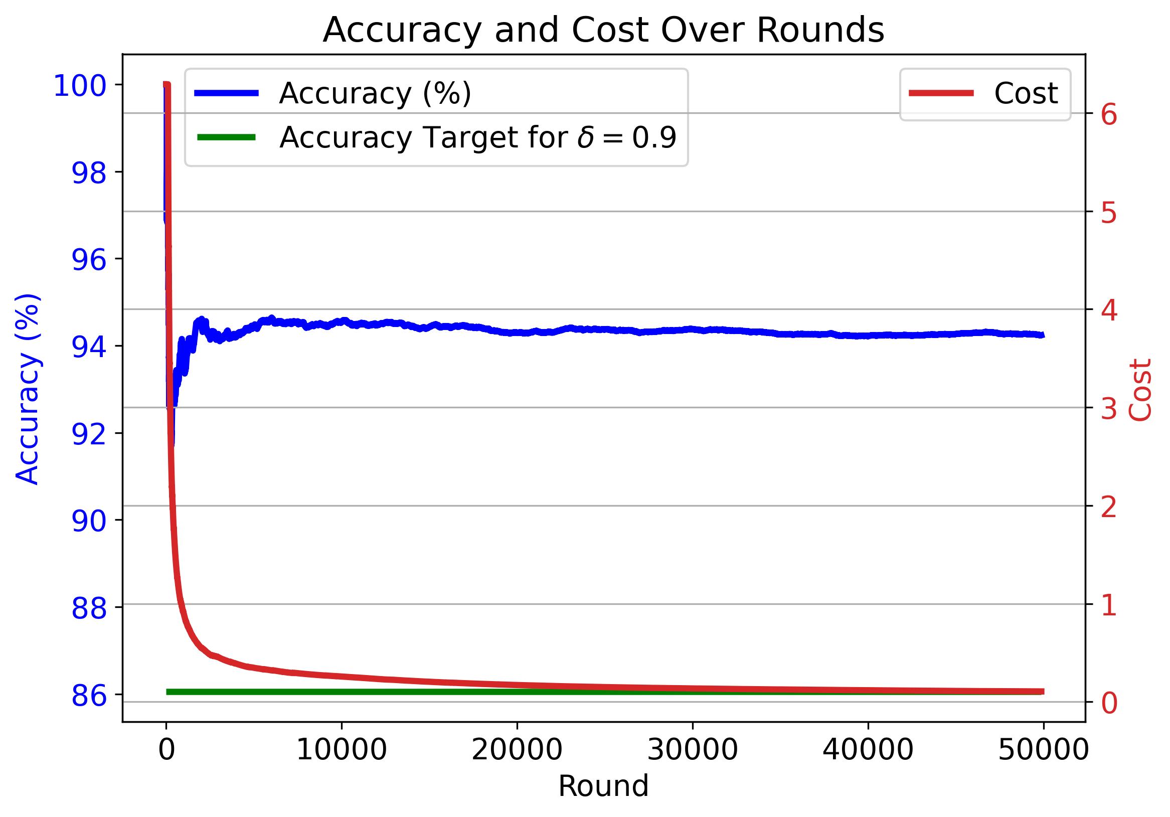
Figure 8: Cumulative average accuracy (blue) and cost (red) of CaMVo ($k_{\min}=1$) on the IMDB Movie Reviews Dataset across rounds for various confidence thresholds $\delta$. The green line marks each $\delta$-specific target accuracy.

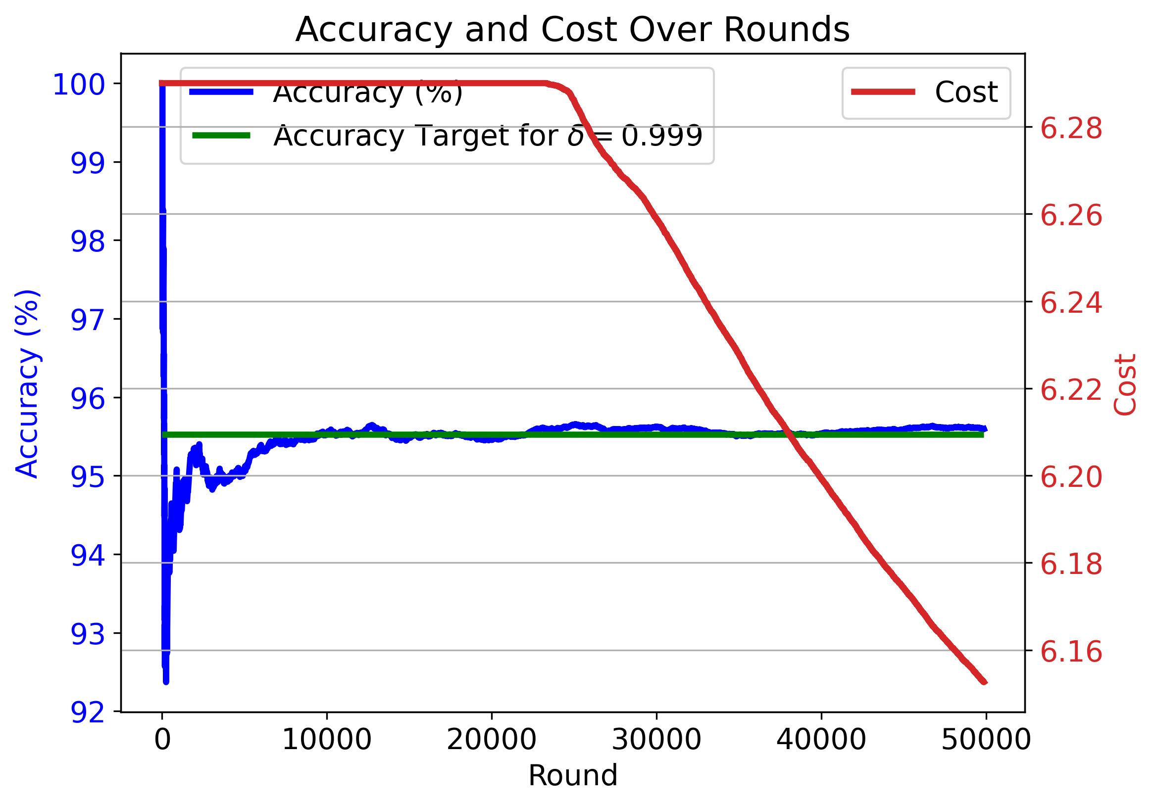
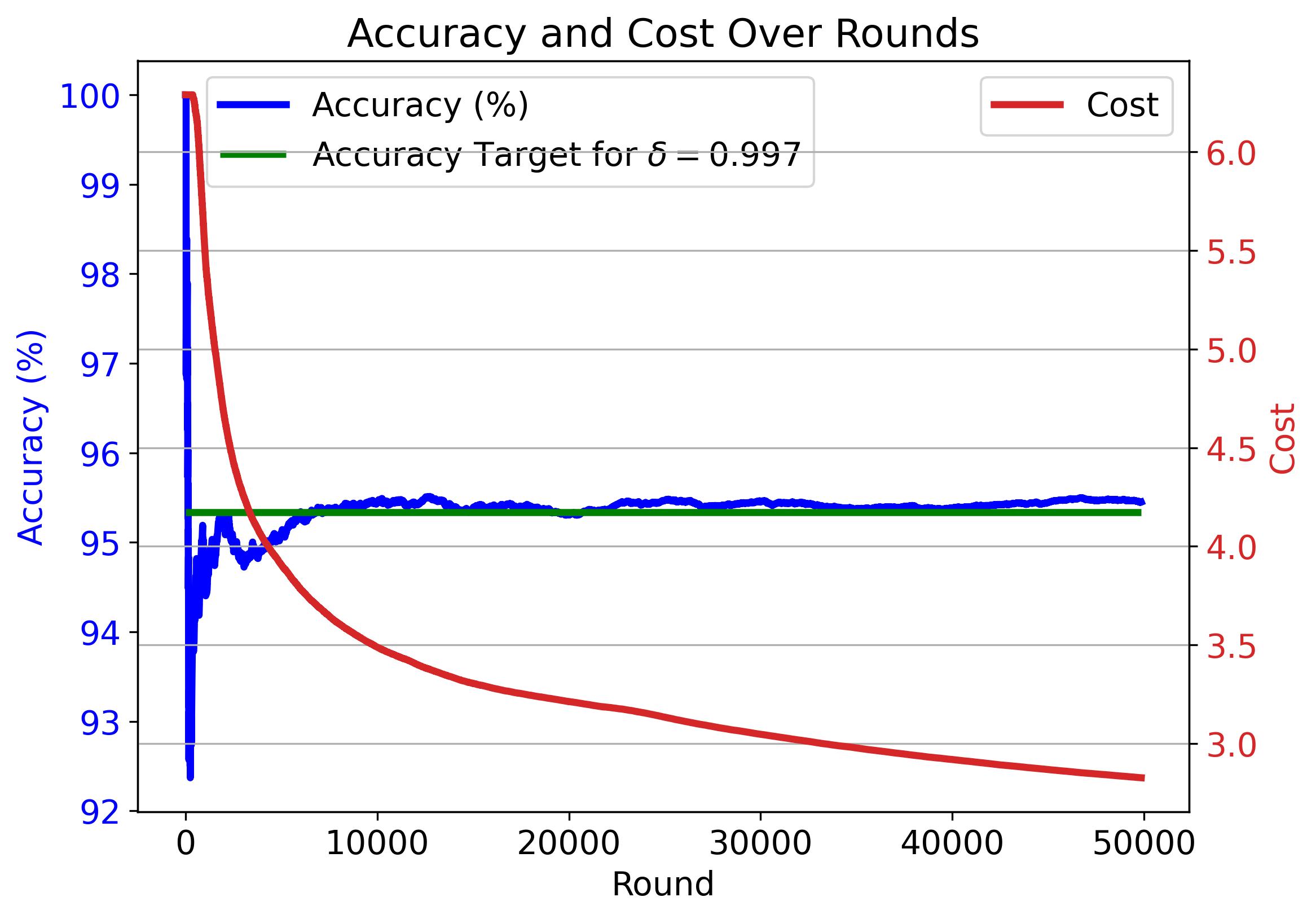
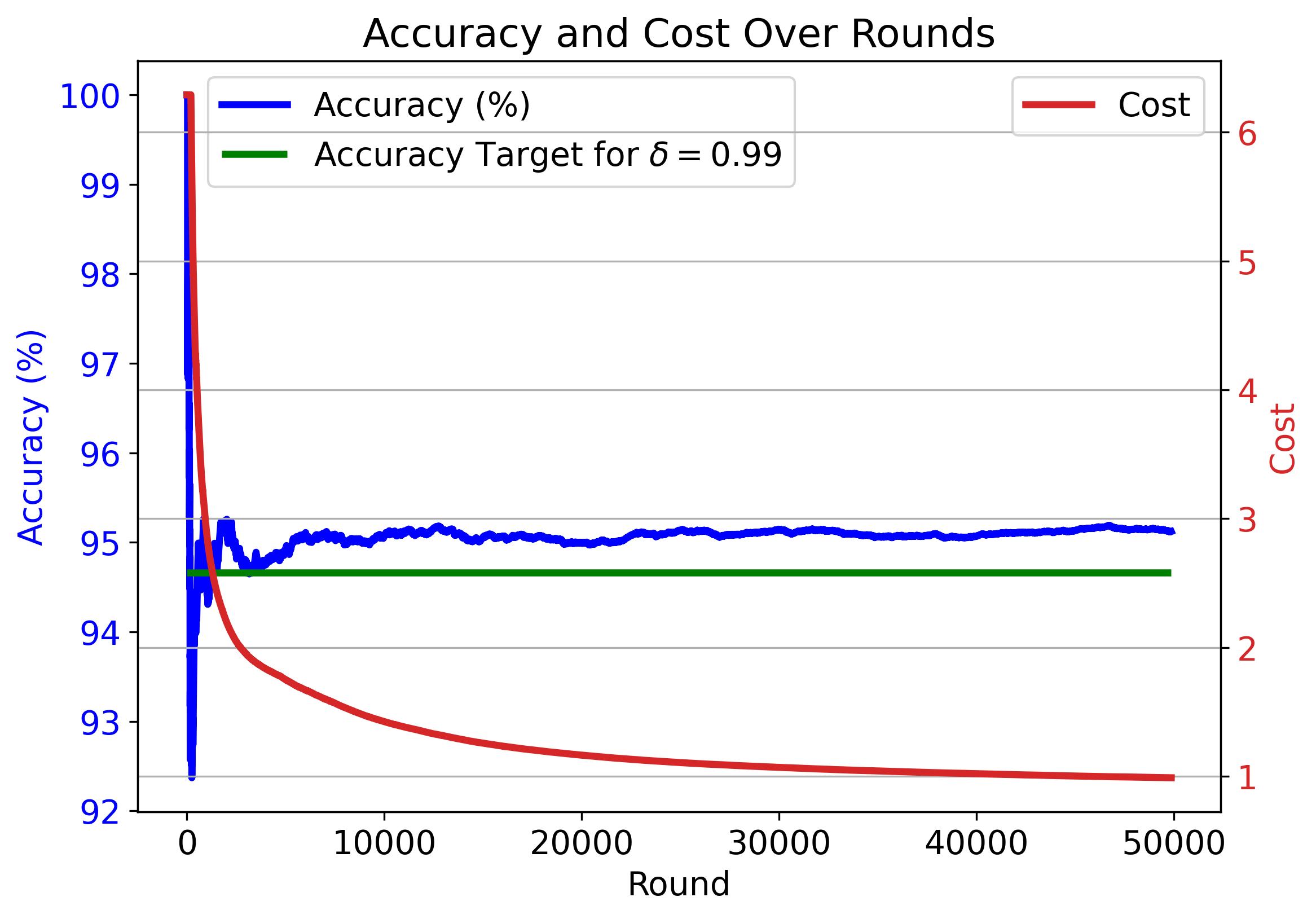
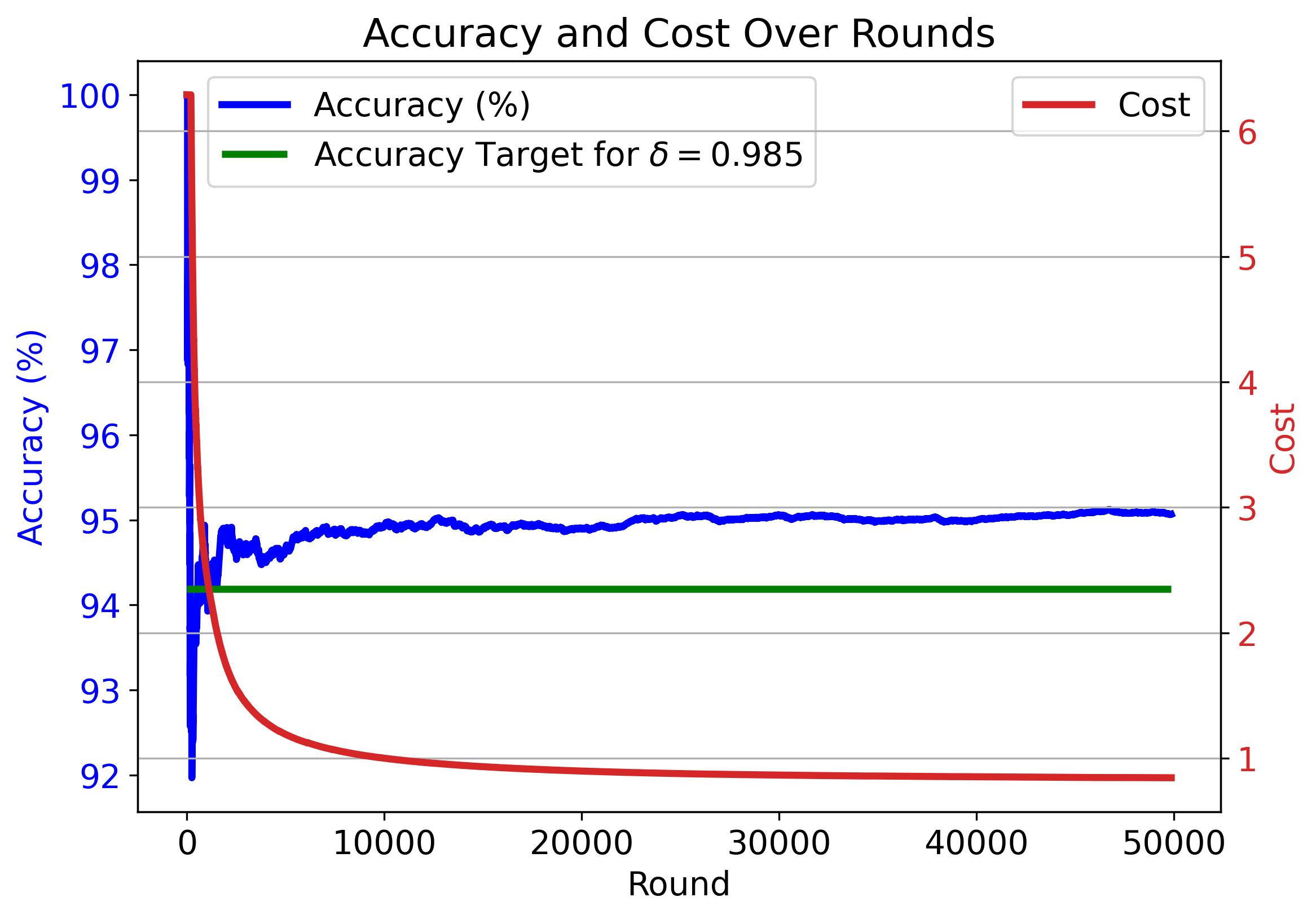
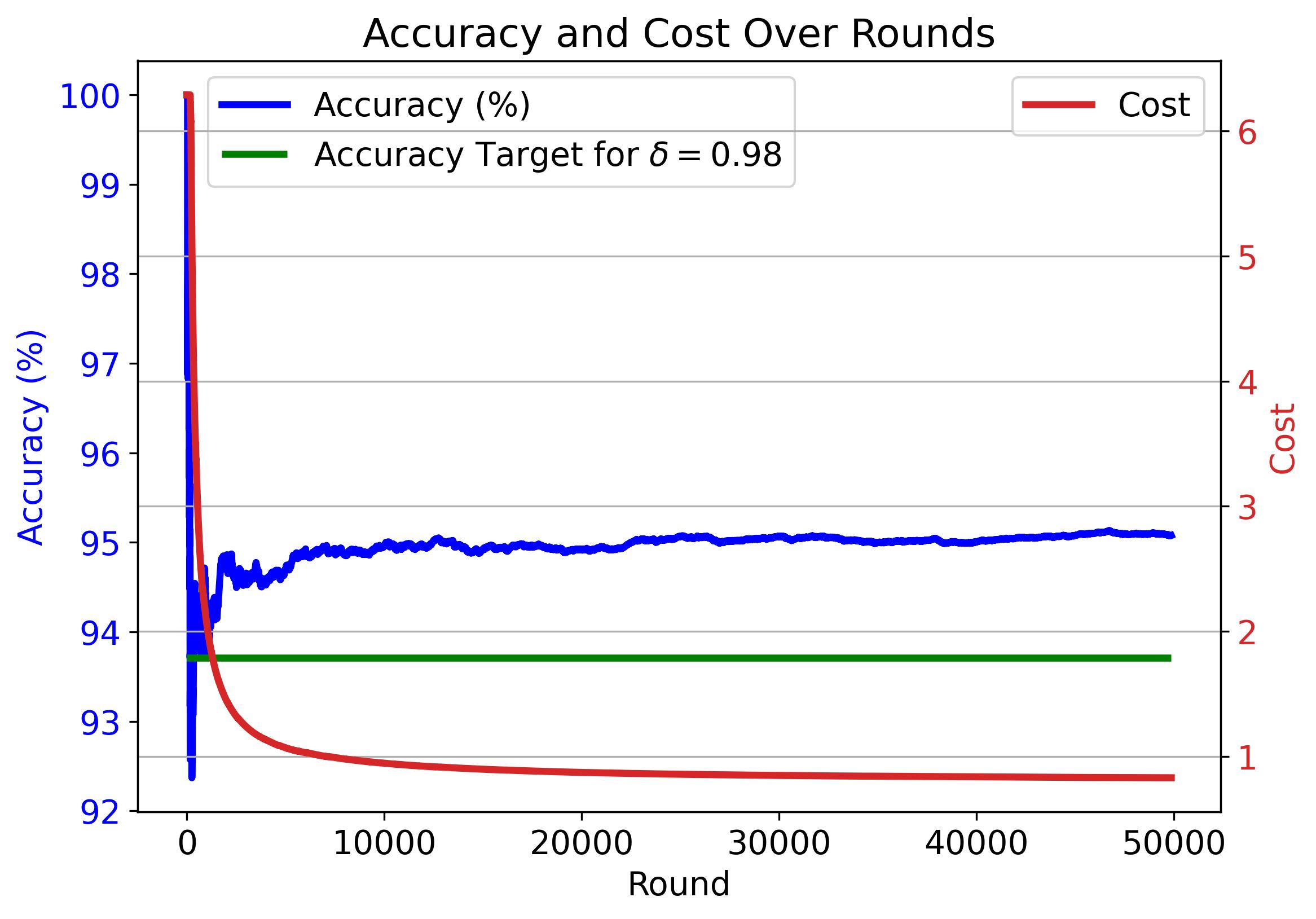
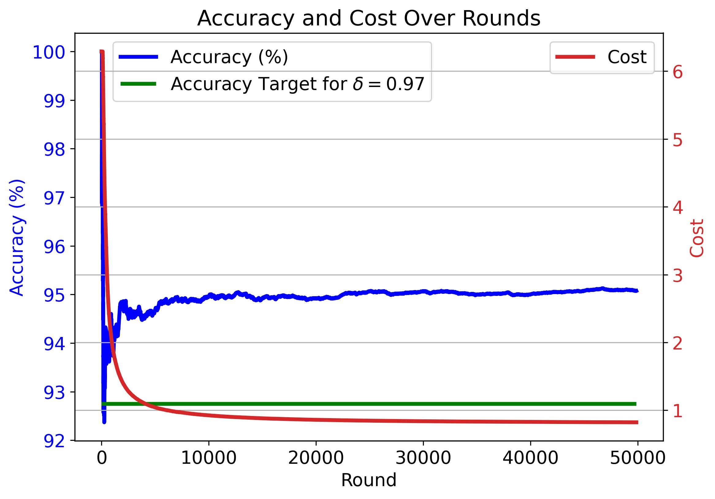
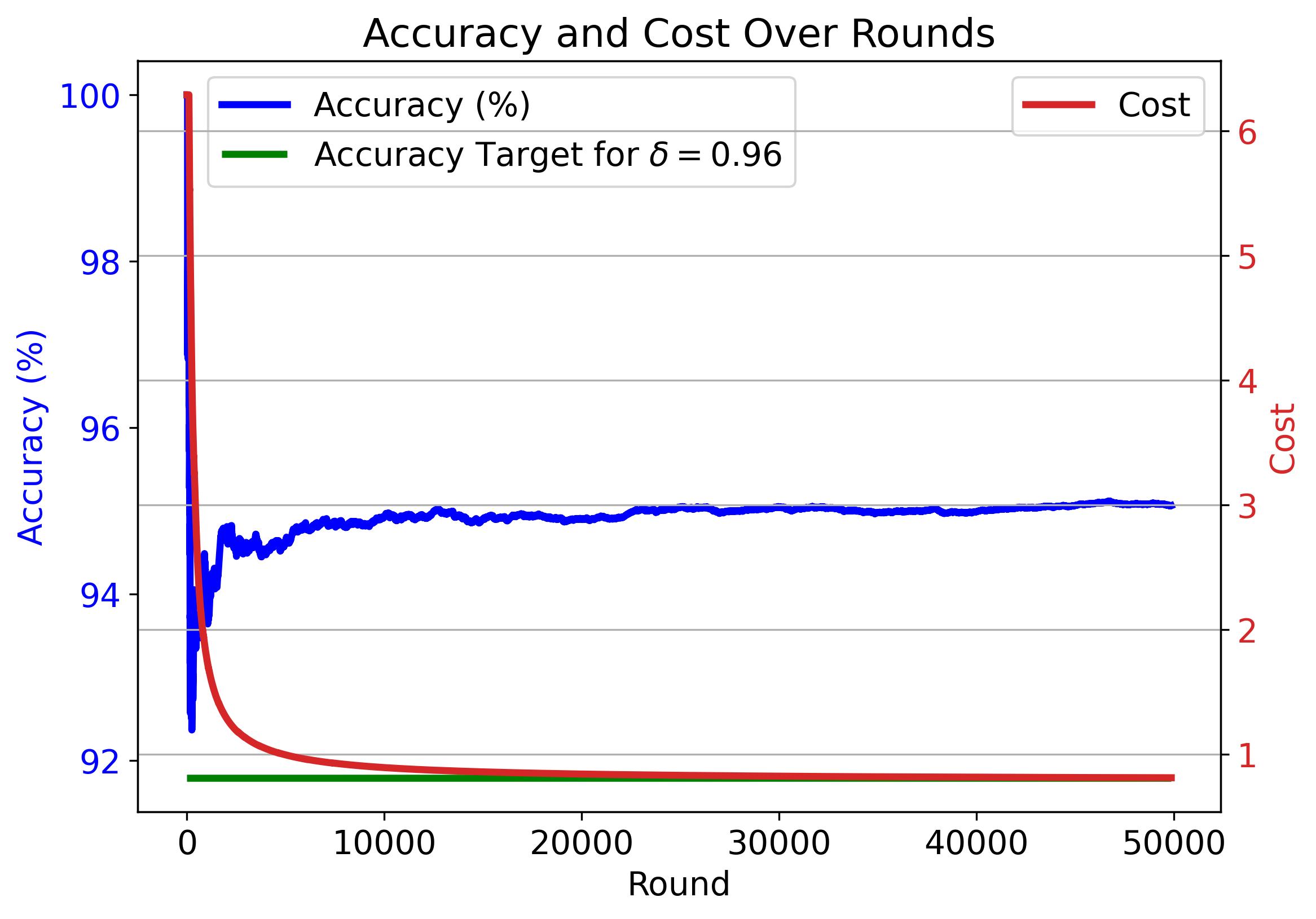
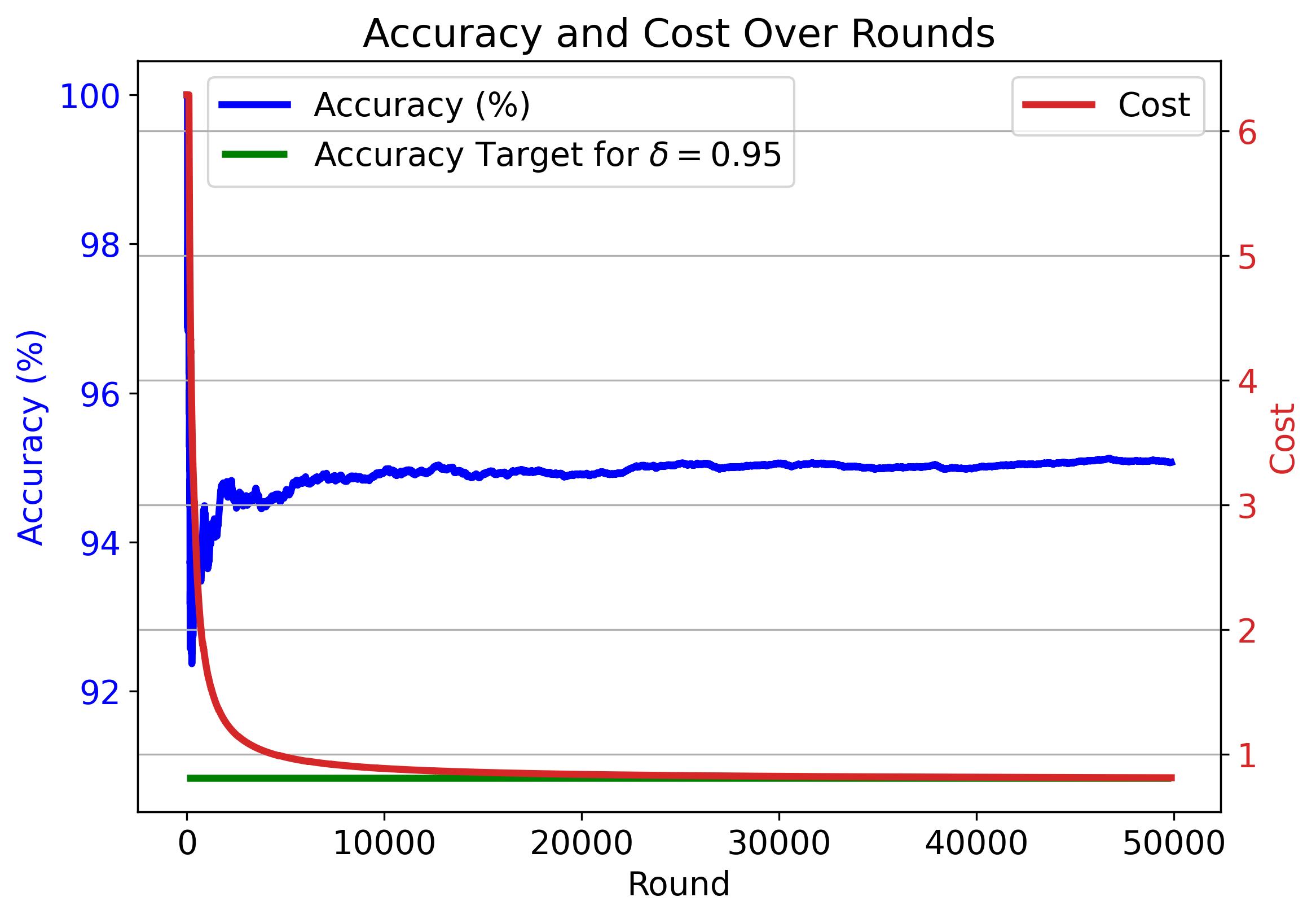
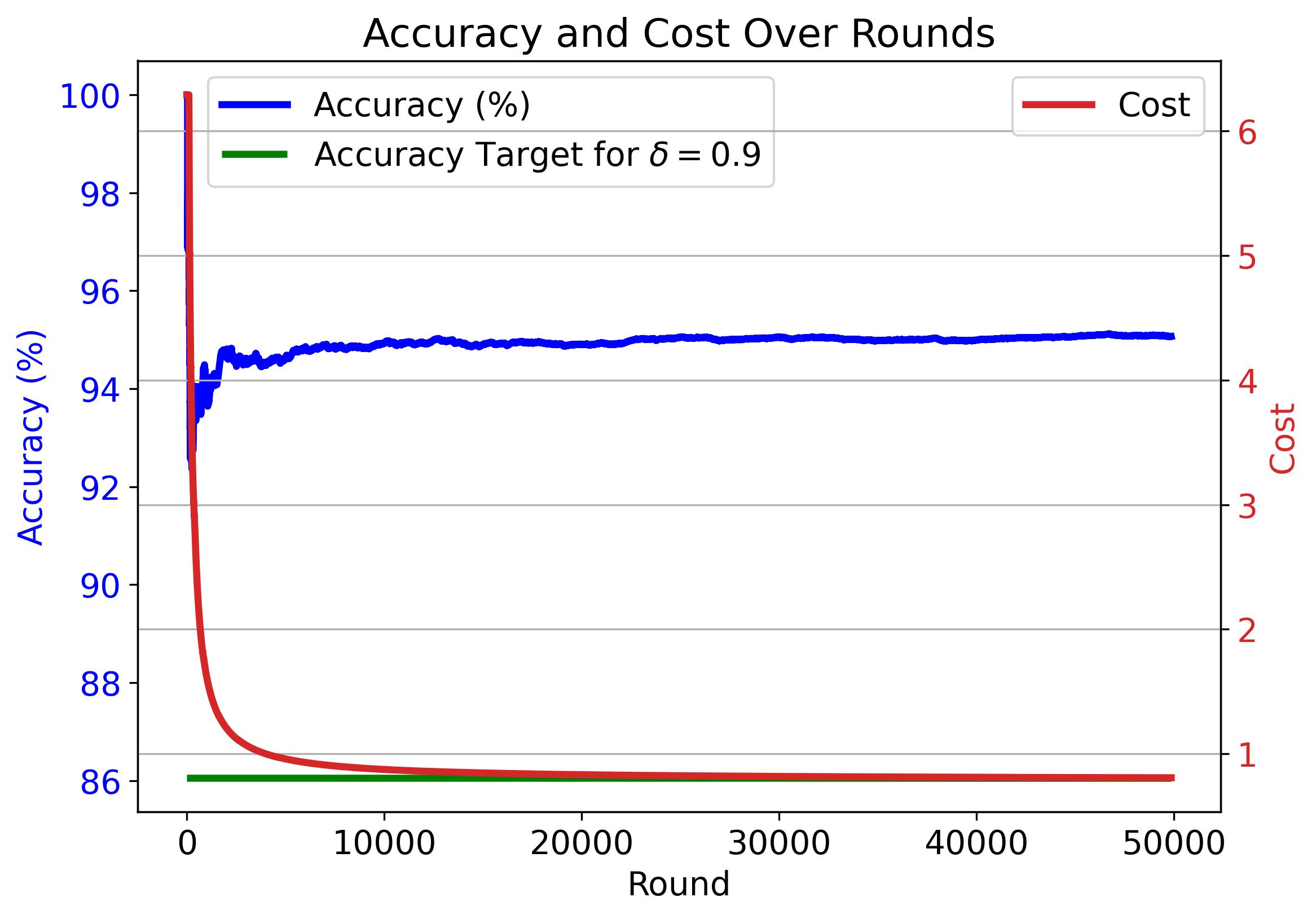
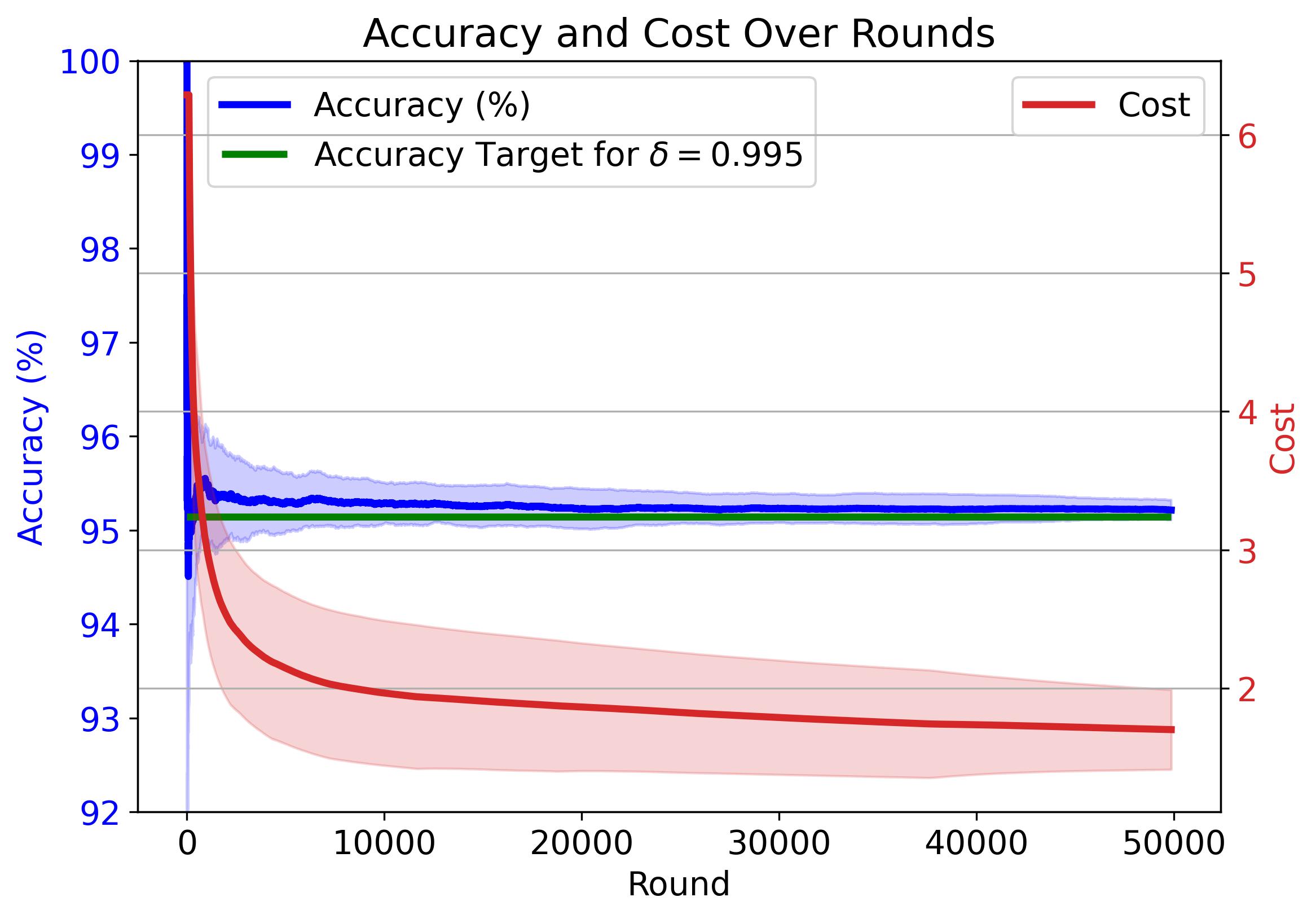
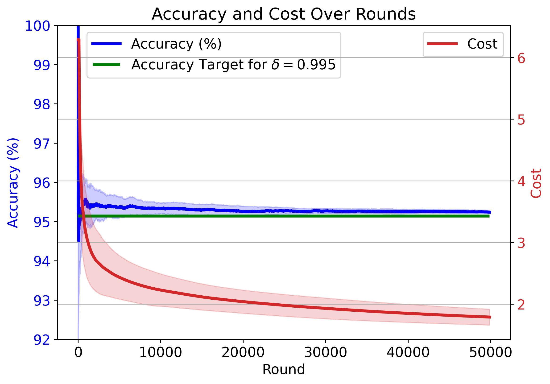
Figure 9: Cumulative average accuracy (blue) and cost (red) of CaMVo ($k_{\min}=3$) on the IMDB Movie Reviews Dataset across rounds for various confidence thresholds $\delta$. The green line marks each $\delta$-specific target accuracy.

Figure 10: Mean (solid lines) and one-standard-deviation bands (shading) of CaMVo’s cumulative average accuracy (blue) and cost (red) over 20 random shuffles of MMLU when $\delta=0.995$ , $k_{\min}=1$ (Left); and $\delta=0.995$ , $k_{\min}=1$ (Right). The green line indicates the accuracy target of $95.14\%$ for $\delta=0.995$.

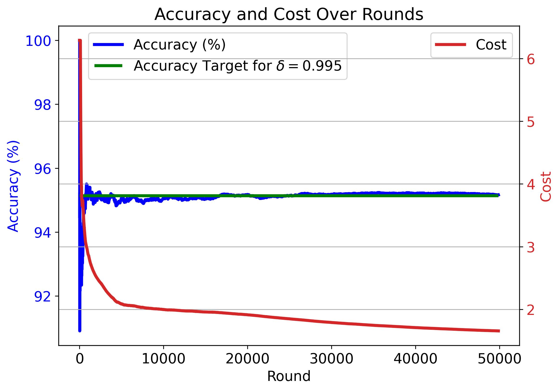
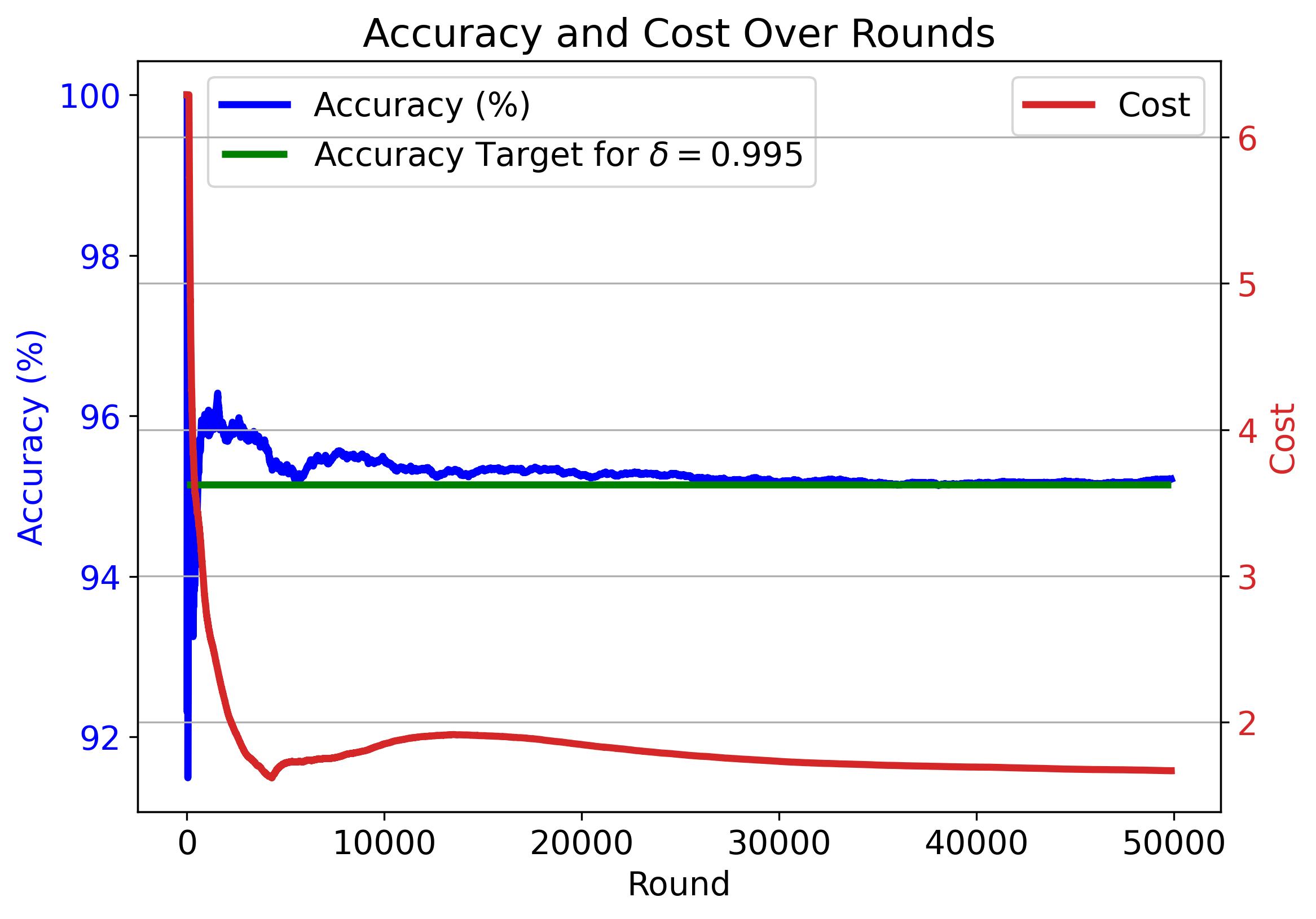
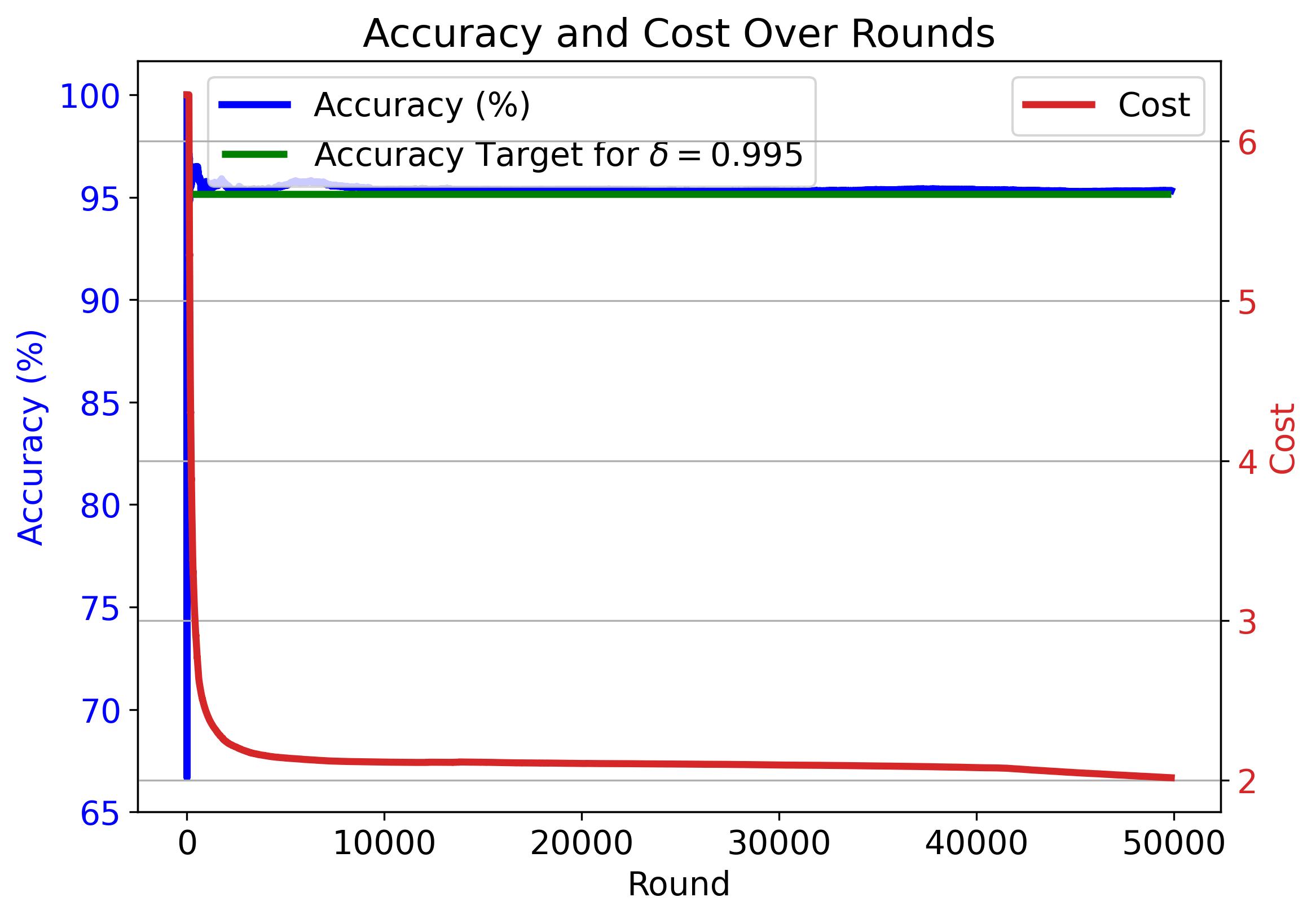
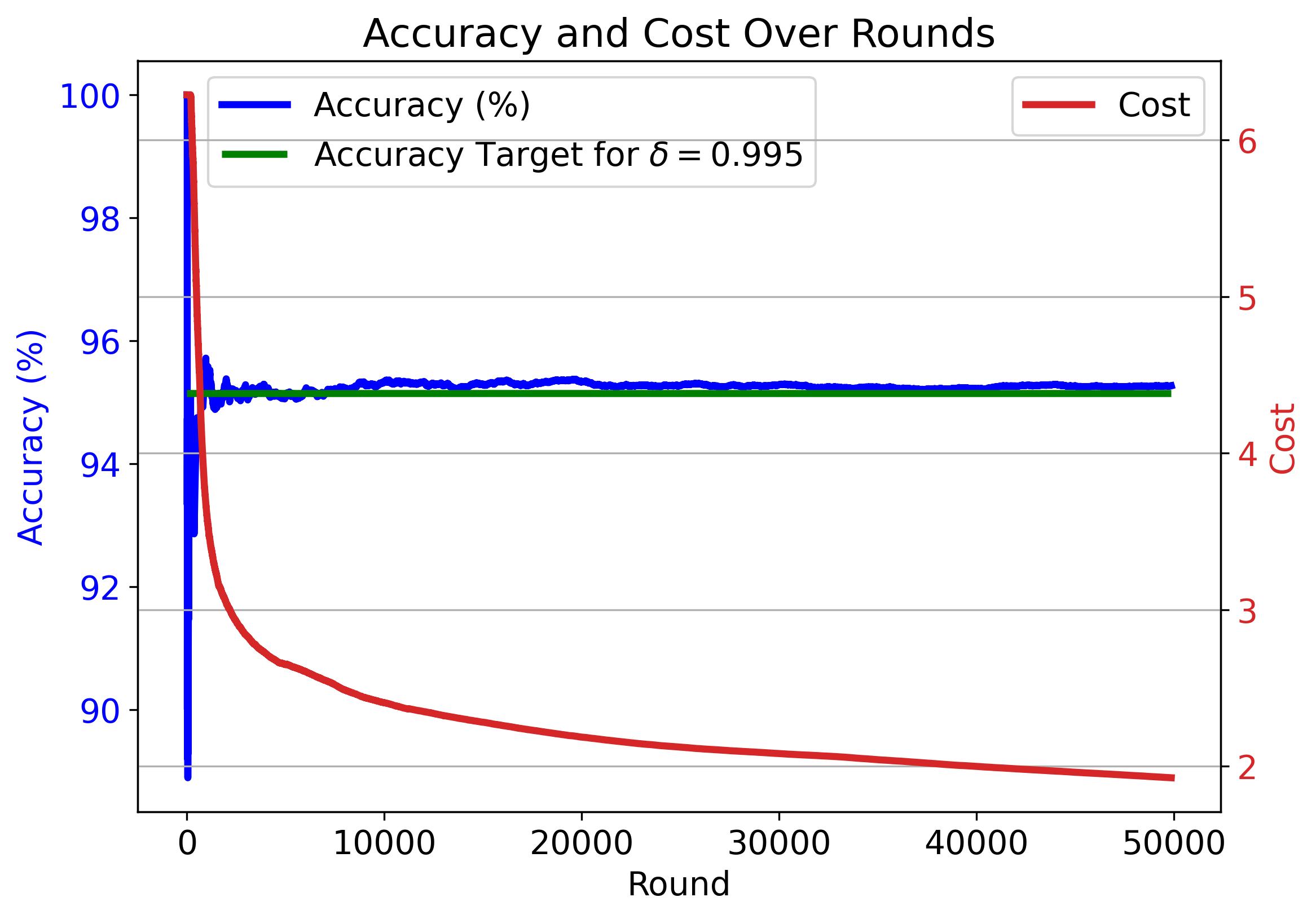
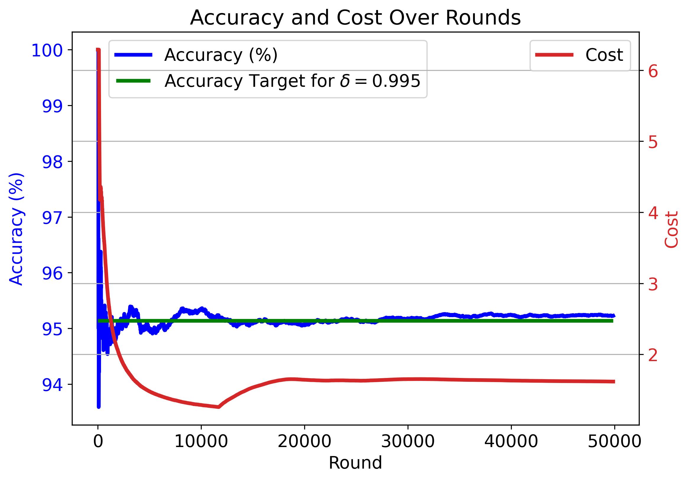
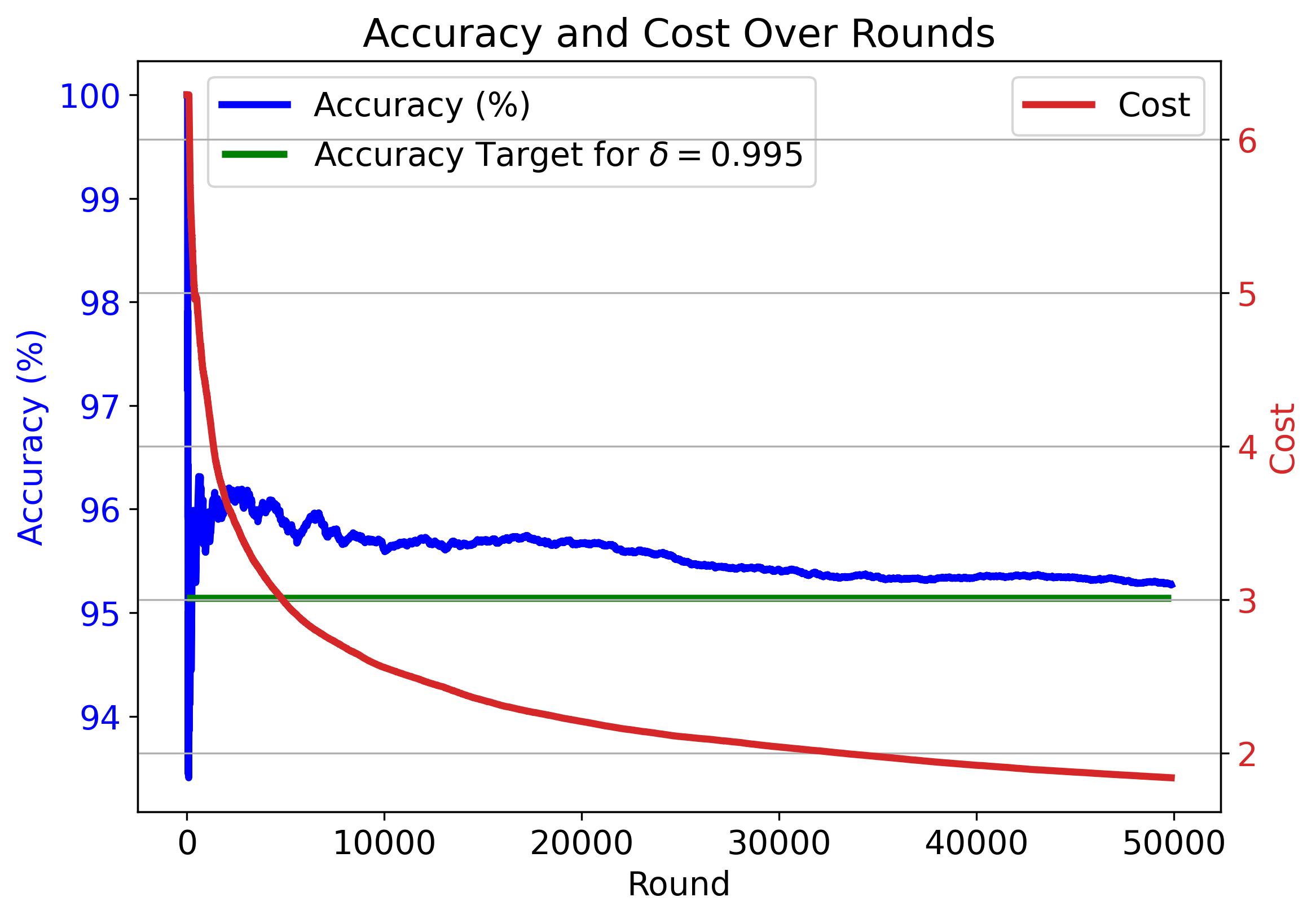
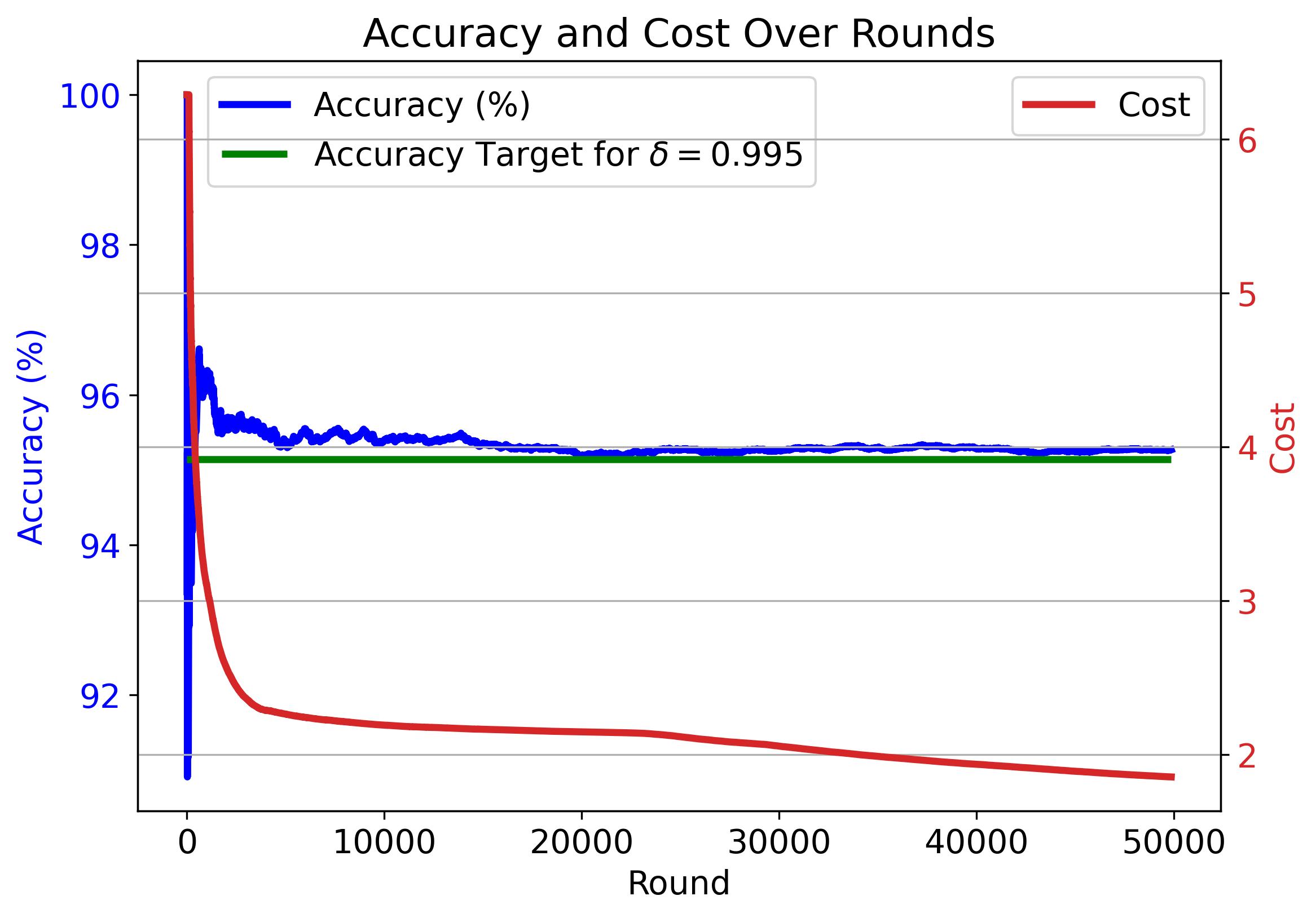
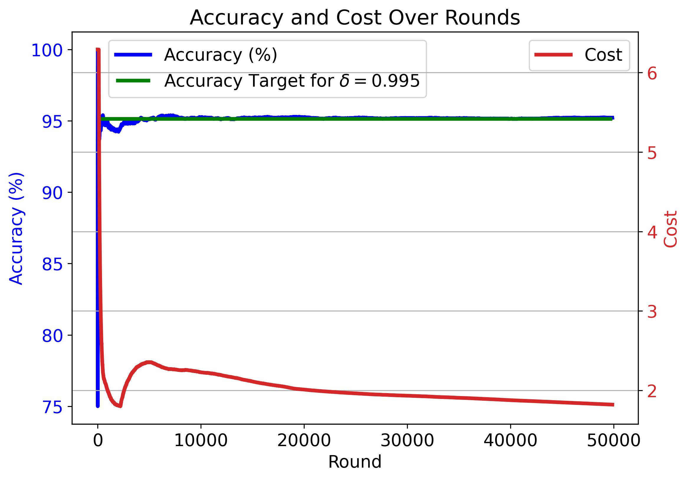
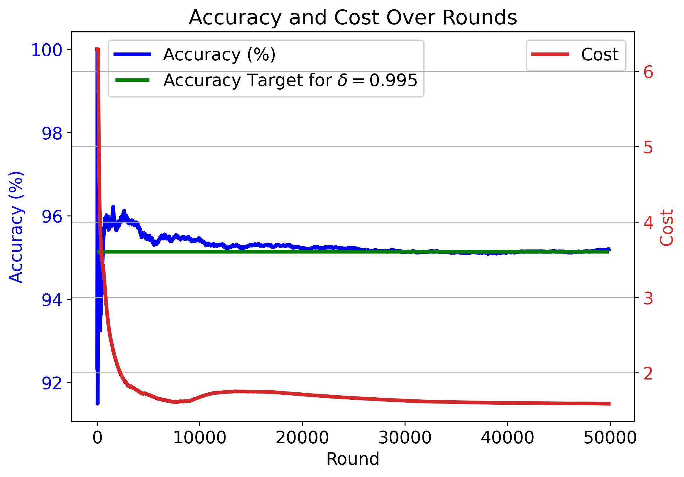
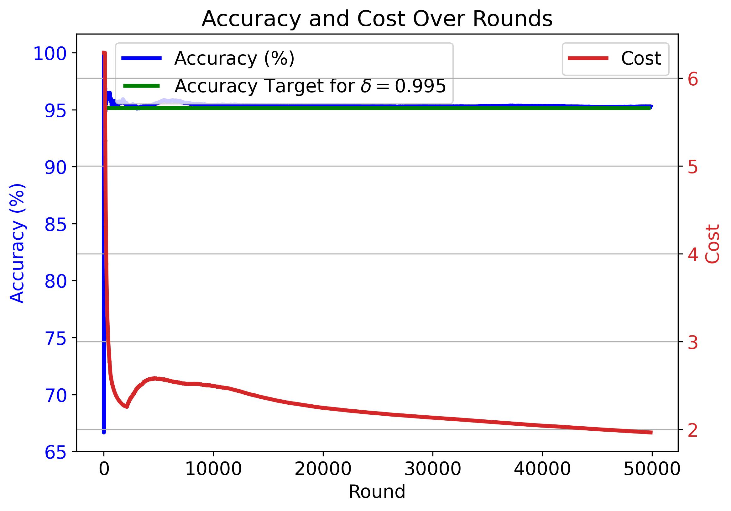
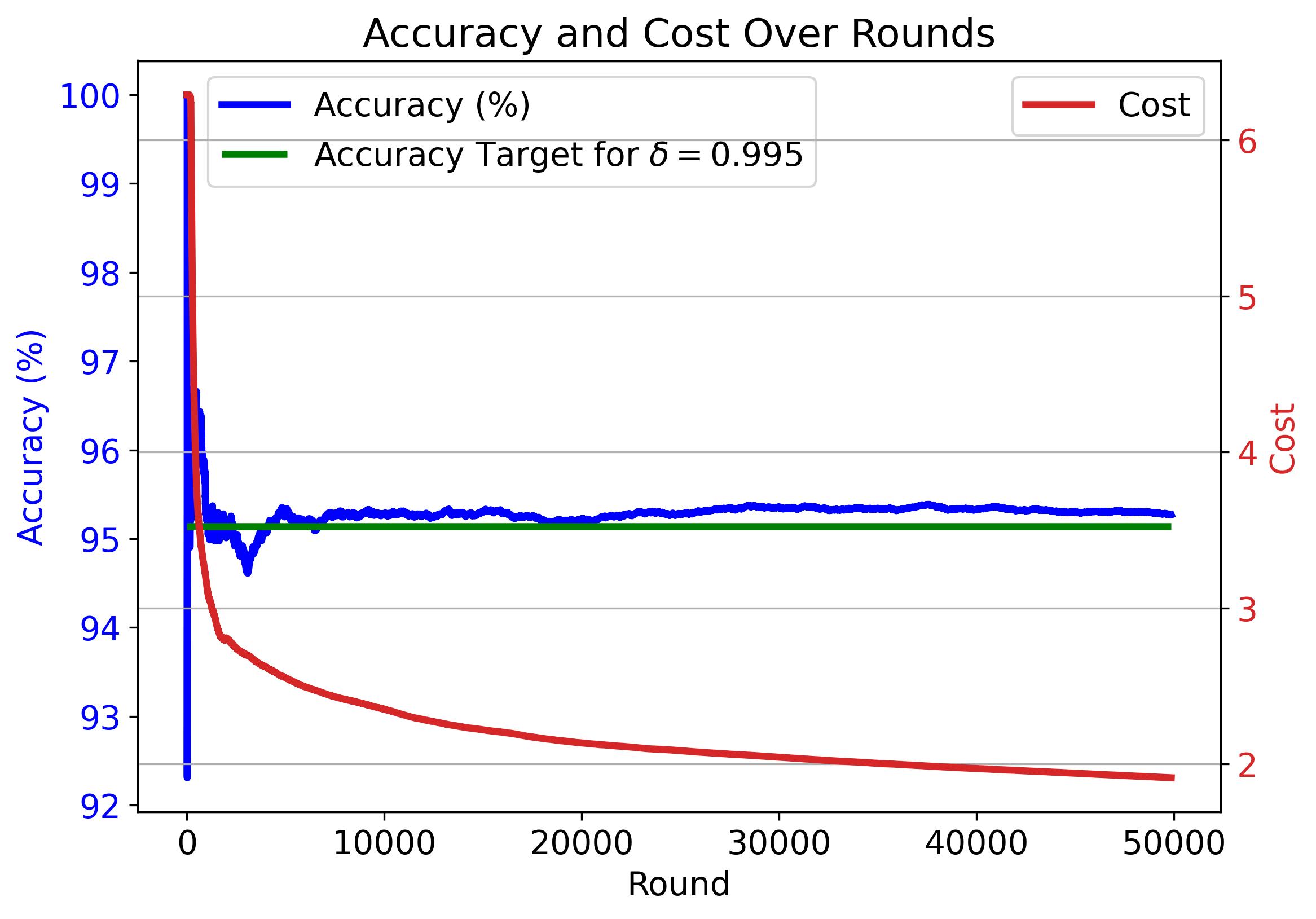
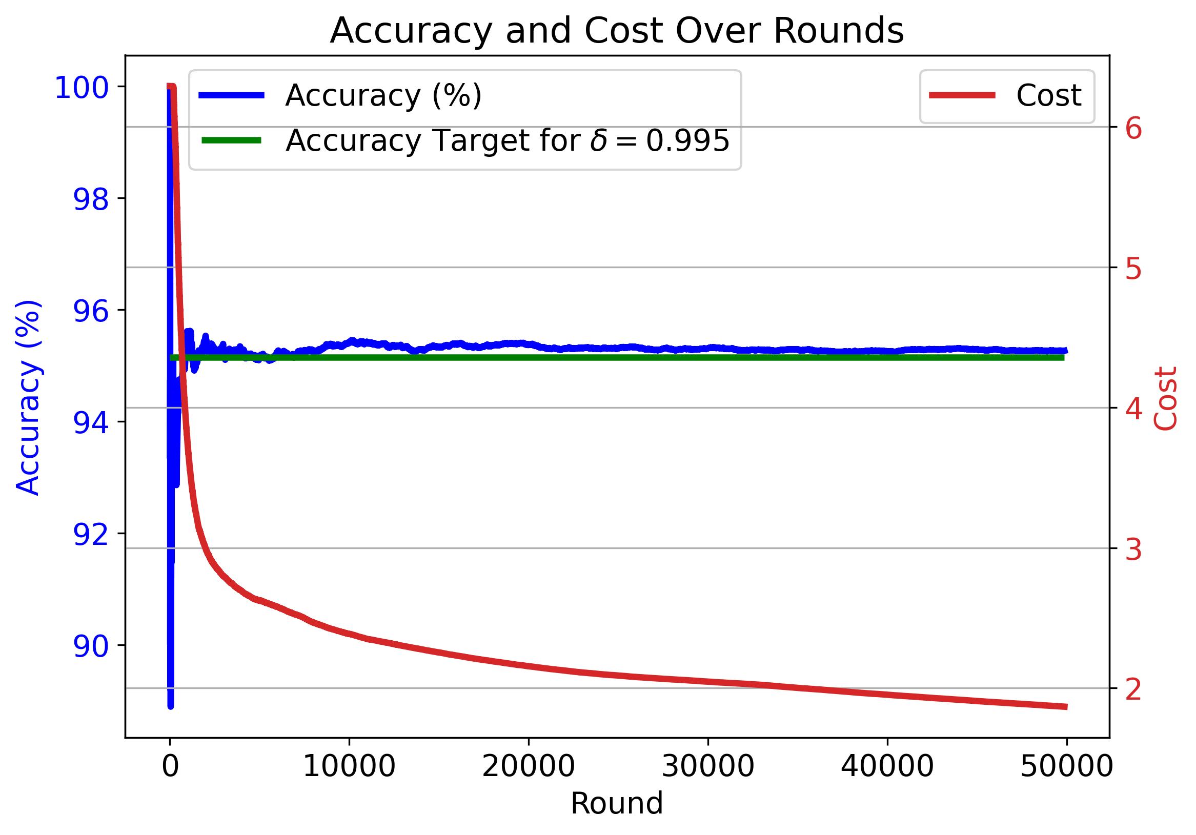
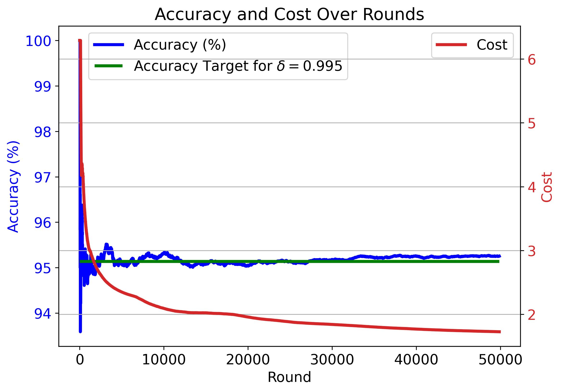
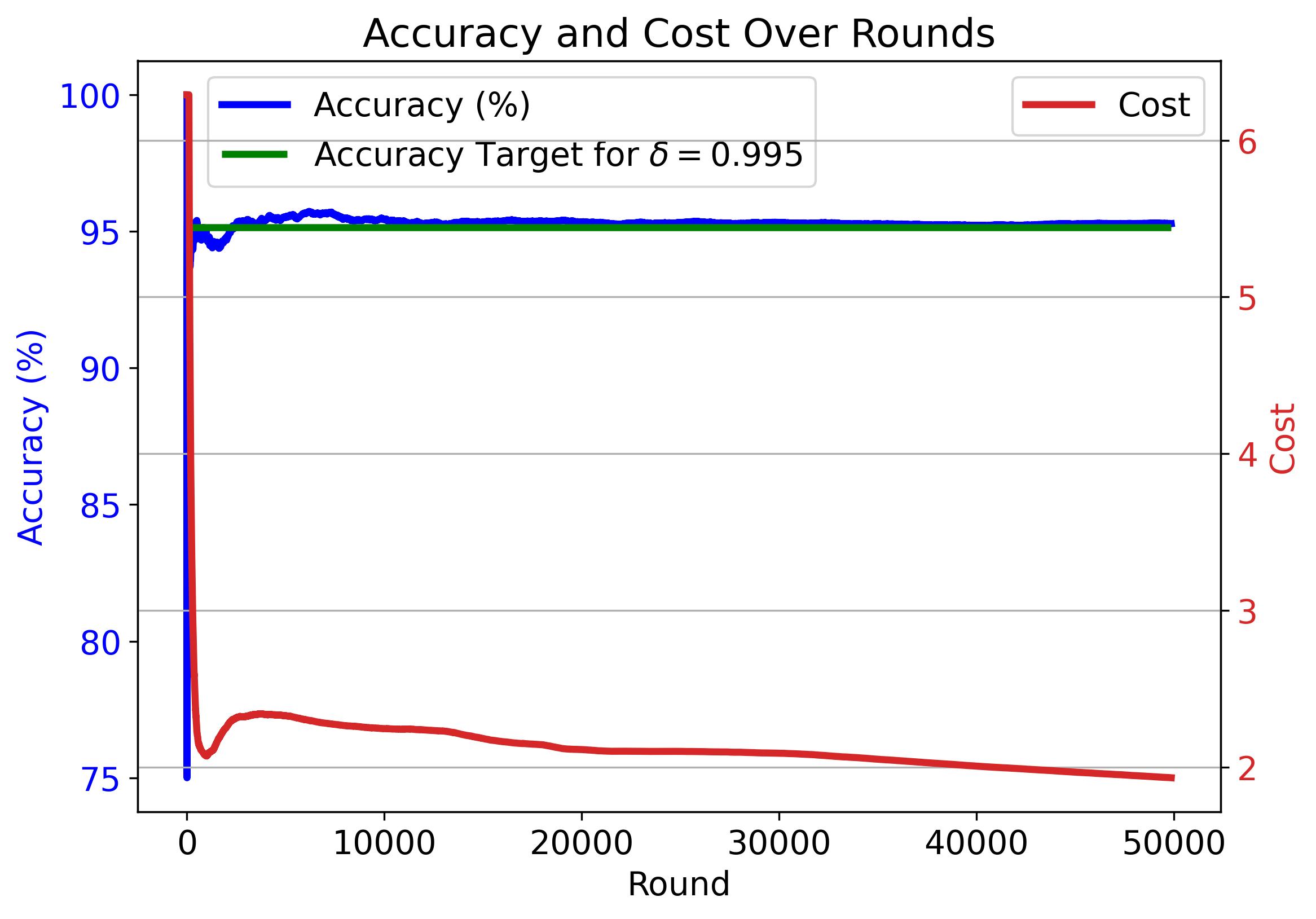
Figure 11: Cumulative average accuracy (blue) and cost (red) of CaMVo with $\delta=0.96$, $k_{\min}=1$ under nine different permutations of the dataset. The green line marks each $\delta$-specific target accuracy.

Figure 12: Cumulative average accuracy (blue) and cost (red) of CaMVo with $\delta=0.96$, $k_{\min}=3$ under nine different permutations of the dataset. The green line marks each $\delta$-specific target accuracy.

Figure 8 visualizes CaMVo’s learning trajectories on IMDB for $k_{\min}=1$ across all the confidence thresholds $\delta$ values reported in Table 4. In all cases, CaMVo begins by querying larger, higher-cost ensembles to obtain reliable performance estimates, then rapidly shifts to cost-optimal subsets once the lower-confidence bounds converge. This transition yields a sharp decline in cost while maintaining accuracy above the target line.

At the extreme threshold $\delta=0.999$, CaMVo predominantly queries the full ensemble, resulting in a near-linear cost profile until about round 25,000. For $\delta\leq 0.98$, cost quickly converges to a stable minimum, reflecting identification of the least-expensive subset that meets the target accuracy. Across all plots, CaMVo achieves or exceeds the respective accuracy target. For very high thresholds ($\delta\geq 0.995$), final accuracy hovers just above the threshold, as expected; as $\delta$ decreases, the accuracy surplus grows. Below $\delta=0.96$, accuracy plateaus at approximately 94.06%, corresponding to the performance of the single cheapest model (‘llama-3.1-8b’).

Overall, these results demonstrate CaMVo’s ability to balance exploration and exploitation, swiftly discover cost-effective subsets, and reliably satisfy the target accuracy requirements.

Figure 10 presents CaMVo’s learning curves under varying confidence thresholds $\delta$ with $k_{\min}=3$. Similar to the $k_{\min}=1$ case, CaMVo initially selects larger, more expensive ensembles to obtain reliable performance estimates, then quickly transitions to lower-cost subsets as the lower confidence bounds stabilize. For $\delta\geq 0.99$, the cost and accuracy trajectories are nearly identical to those observed with $k_{\min}=1$. When $\delta\leq 0.985$, CaMVo settles on the lowest-cost subset of three LLMs, and the plots when $\delta\leq 0.985$ are almost-identical.

To assess CaMVo’s sensitivity to dataset ordering, Figure 10 plots the mean cumulative accuracy and cost curves (solid lines) for MMLU when $\delta=0.995$ , $k_{\min}=1$ (Left); and $\delta=0.995$ , $k_{\min}=1$ (Right), averaged over 20 random shuffles. Shaded regions indicate one standard deviation. Although the accuracy band starts wide, which reflects both the initial exploration and also the varying mixes of ’easier’ and ’harder’ instances; this rapidly contracts over time, confirming CaMVo’s reliable attainment of the target accuracy across permutations. The cost band likewise narrows, demonstrating stable convergence to low-cost ensembles. Notably, the accuracy variability remains much smaller than the cost variability, as CaMVo does not optimize toward a fixed cost. Comparing $k_{\min}=1$ and $k_{\min}=3$, it can be seen that both the cost and accuracy bands are narrower, as there are less available subsets to choose when $k_{\min}=3$.

Figure 12 further investigates ordering effects by overlaying nine individual runs from these permutations. In every run, CaMVo exceeds the 95.14% accuracy target while driving per-round cost below $2.10, corroborating that its exploration–exploitation strategy, and the resulting cost–accuracy performance is effectively invariant to the input sequence. Figure 12 presents analogous results for the $k_{\min}=3$ setting, confirming similar robustness to input permutations.

References

- Anthropic [2024] Anthropic. Claude 3 technical overview. https://www.anthropic.com/index/claude-3, 2024. Accessed: 2025-04-24.
- Chen et al. [2024] Lingjiao Chen, Jared Quincy Davis, Boris Hanin, Peter Bailis, Ion Stoica, Matei A Zaharia, and James Y Zou. Are more llm calls all you need? towards the scaling properties of compound ai systems. Advances in Neural Information Processing Systems, 37:45767–45790, 2024.
- Ding et al. [2024] Dujian Ding, Ankur Mallick, Chi Wang, Robert Sim, Subhabrata Mukherjee, Victor Ruhle, Laks VS Lakshmanan, and Ahmed Hassan Awadallah. Hybrid llm: Cost-efficient and quality-aware query routing. arXiv preprint arXiv:2404.14618, 2024.
- Errica et al. [2024] Federico Errica, Giuseppe Siracusano, Davide Sanvito, and Roberto Bifulco. What did i do wrong? quantifying llms’ sensitivity and consistency to prompt engineering. arXiv preprint arXiv:2406.12334, 2024.
- Hendrycks et al. [2021a] Dan Hendrycks, Collin Burns, Steven Basart, Andrew Critch, Jerry Li, Dawn Song, and Jacob Steinhardt. Aligning ai with shared human values. Proceedings of the International Conference on Learning Representations (ICLR), 2021a.
- Hendrycks et al. [2021b] Dan Hendrycks, Collin Burns, Steven Basart, Andy Zou, Mantas Mazeika, Dawn Song, and Jacob Steinhardt. Measuring massive multitask language understanding. Proceedings of the International Conference on Learning Representations (ICLR), 2021b.
- Kadavath et al. [2022] Saurav Kadavath, Tom Conerly, Amanda Askell, Tom Henighan, Dawn Drain, Ethan Perez, Nicholas Schiefer, Zac Hatfield-Dodds, Nova DasSarma, Eli Tran-Johnson, et al. Language models (mostly) know what they know. arXiv preprint arXiv:2207.05221, 2022.
- Li and Yu [2014] Hongwei Li and Bin Yu. Error rate bounds and iterative weighted majority voting for crowdsourcing. arXiv preprint arXiv:1411.4086, 2014.
- Li et al. [2024a] Jia Li, Yuqi Zhu, Yongmin Li, Ge Li, and Zhi Jin. Showing llm-generated code selectively based on confidence of llms. arXiv preprint arXiv:2410.03234, 2024a.
- Li et al. [2024b] Junyou Li, Qin Zhang, Yangbin Yu, Qiang Fu, and Deheng Ye. More agents is all you need. arXiv preprint arXiv:2402.05120, 2024b.
- Li et al. [2010] Lihong Li, Wei Chu, John Langford, and Robert E Schapire. A contextual-bandit approach to personalized news article recommendation. In Proceedings of the 19th international conference on World wide web, pages 661–670, 2010.
- Maas et al. [2011] Andrew L. Maas, Raymond E. Daly, Peter T. Pham, Dan Huang, Andrew Y. Ng, and Christopher Potts. Learning word vectors for sentiment analysis. In Proceedings of the 49th Annual Meeting of the Association for Computational Linguistics: Human Language Technologies, pages 142–150, Portland, Oregon, USA, June 2011. Association for Computational Linguistics. URL http://www.aclweb.org/anthology/P11-1015.
- Meta [2024] Meta. Llama-3 models. https://www.llama.com/models/llama-3/, 2024. Accessed: 2025-04-24.
- Naveed et al. [2023] Humza Naveed, Asad Ullah Khan, Shi Qiu, Muhammad Saqib, Saeed Anwar, Muhammad Usman, Naveed Akhtar, Nick Barnes, and Ajmal Mian. A comprehensive overview of large language models. arXiv preprint arXiv:2307.06435, 2023.
- Nguyen et al. [2024] Quang H Nguyen, Duy C Hoang, Juliette Decugis, Saurav Manchanda, Nitesh V Chawla, and Khoa D Doan. Metallm: A high-performant and cost-efficient dynamic framework for wrapping llms. arXiv preprint arXiv:2407.10834, 2024.
- OpenAI [2024] OpenAI. Openai models. https://platform.openai.com/docs/models, 2024. Accessed: 2025-04-24.
- Petrović et al. [2020] Nataša Petrović, Gabriel Moyà-Alcover, Javier Varona, and Antoni Jaume-i Capó. Crowdsourcing human-based computation for medical image analysis: A systematic literature review. Health informatics journal, 26(4):2446–2469, 2020.