Runge–Kutta Methods and Stiff Order Conditions for Semilinear ODEs

Abstract

Classical convergence theory of Runge–Kutta methods assumes that the time step is small relative to the Lipschitz constant of the ordinary differential equation (ODE). For stiff problems, that assumption is often violated, and a problematic degradation in accuracy, known as order reduction, can arise. High stage order methods can avoid order reduction, but they must be fully implicit. For linear problems, weaker stiff order conditions exist and are compatible with computationally efficient methods, i.e., explicit or diagonally implicit. This work develops a new theory of stiff order conditions and convergence for semilinear ODEs, consisting of a stiff linear term and a non-stiff nonlinear term. New semilinear order conditions are formulated in terms of orthogonality relations enumerated by rooted trees. Novel, optimized diagonally implicit methods are constructed that satisfy these semilinear conditions. Numerical results demonstrate that for a broad class of relevant nonlinear test problems, these new methods successfully mitigate order reduction and yield highly accurate numerical approximations.

MSC Classification]65L05, 65L06, 65L20, 65L70, 65M20

1 Introduction

This paper concerns ordinary differential equations (ODEs) of the semilinear form

$$y^{\prime}(t)=f(y(t))=Jy(t)+g(y(t)),\quad y(t_{0})=y_{0},\quad t\in[t_{0},t_{\mathrm{f}}],$$ (1)

where $y(t)\in\mathbb{R}^{N}$. The linear term $Jy$ may be stiff and involves a constant coefficient matrix $J\in\mathbb{R}^{N\times N}$. The term $g(y(t))$ is assumed to be non-stiff but can be nonlinear. Of particular interest are initial boundary value problems which, after discretization in space, are often of the form 1.

We use the Runge–Kutta family of one-step methods for the numerical integration of 1. For a general right-hand side function $f$, they are given by

$$Y_{n,i} =y_{n}+h\sum_{j=1}^{s}a_{i,j}f(Y_{n,j}),\qquad i=1,\dots,s,$$ (2a)

$$y_{n+1} =y_{n}+h\sum_{i=1}^{s}b_{i}f(Y_{n,i}),$$ (2b)

where $h$ is the time step on the uniform time grid $t_{n}=t_{0}+nh$, the intermediate stages are denoted by $Y_{n,i}$, and $y_{n}$ is an approximation to the exact solution $y(t_{n})$. Associated with this method are the $s\times s$ matrix $A=(a_{i,j})_{i,j=1}^{s}$, weight vector $b=(b_{i})_{i=1}^{s}$, and abscissa vector $c=(c_{i})_{i=1}^{s}$; the latter is defined in this paper by the standard row simplifying assumption $c=A\mathbbm{1}$, where $\mathbbm{1}=[1,\dots,1]^{T}\in\mathbb{R}^{s}$.

Unfortunately, in the presence of stiffness, Runge–Kutta methods may converge at a rate less than that predicted by their classical order, denoted throughout as $p$. This order reduction phenomenon was demonstrated in the seminal work of Prothero and Robinson [prothero1974stability].

In response, B-convergence [frank1981concept], [dekker1984stability, p. 201], [scholz1989order, p. 219] was introduced to provide global error bounds that hold uniformly with respect to stiffness. For Runge–Kutta methods applied to nonlinear problems, B-convergence theory relies heavily on the following simplifying assumptions (see [frank1985order, Lemma 2.1], [burrage1987order, Theorem 2.2], and [hairer1996solving, Section IV.15]):

$$B(q_{1}): b^{T}c^{k-1} =\frac{1}{k}, \quad k =1,\dots,q_{1},$$ (3a)

$$C(q_{2}): Ac^{k-1} =\frac{c^{k}}{k}, \quad k =1,\dots,q_{2}.$$ (3b)

Here $c^{k}=[c_{1}^{k},\ldots,c_{s}^{k}]^{T}$. The minimum of $q_{1}$ and $q_{2}$ for which 3 holds is known as the stage order. While fully implicit Runge–Kutta methods can attain high stage order, their implementation requires the solution of large, coupled nonlinear algebraic systems at each step. B-convergence results are severely limited for more computationally efficient explicit and diagonally implicit methods because their maximum stage order is one and two, respectively.

One of the first works to investigate B-convergence of Runge–Kutta methods specifically for semilinear problems is [burrage1986study]. Burrage, Hundsdorfer, and Verwer show that stringent nonlinear stability requirements for generic, nonlinear analysis are not needed. Instead, weaker linear stability conditions suffice. Extension to semilinear problems where the linear term is time-dependent were explored in [auzinger1992extension, calvo2000runge]. The B-convergence results in all of these works apply only to high stage order methods. Strehmel and Weiner use a more refined per-stage simplifying assumption in [strehmel1987b] to combat order reduction. Skvortsov has derived order conditions for nonlinear generalizations of the Prothero–Robinson problem (see [skvortsov2003accuracy, Table 3] and [skvortsov2010model, Table 3]). Recently, similar techniques have been extended to differential algebraic equations with a focus on the incompressible Navier–Stokes equations [CaiWanKareem2025].

Outside the class of Runge–Kutta schemes, sharp error analysis for semilinear problems has been explored for exponential integrators [hochbruck2005explicit, luan2013exponential, hochbruck2020convergence], splitting methods [hansen2016high, einkemmer2015overcoming, einkemmer2016overcoming], Rosenbrock methods [lubich1995linearly], and linear multistep methods [hairer1996solving, Section V.8].

In this paper, we introduce a novel B-convergence error analysis which yields sharp order conditions for Runge–Kutta schemes applied to stiff, semilinear ODEs 1. Notably, our semilinear order conditions are weaker than high stage order. The conditions are posed in terms of rational functions of an auxiliary variable, similar to weak stage order conditions [ketcheson2020dirk], but are in one-to-one correspondence with rooted trees, similar to classical, non-stiff order conditions. We construct practical diagonally implicit Runge–Kutta (DIRK) methods which attain up to fifth order B-convergence. This is verified with numerical experiments on a semilinear variant of the Prothero–Robinson problem and several partial differential equations (PDEs). We note that in ODEs for which the nonlinear term is stiff (for instance, the van der Pol oscillator) do not fit into the analysis presented here, and numerical experiments indicate that the methods presented herein do not necessarily alleviate order reduction for such problems.

Before proceeding, we briefly introduce the upcoming sections. Mathematical background and assumptions necessary for the paper are provided in Section 2. Then, Section 3 contains our primary convergence results and order condition theory. Section 4 concerns the design and derivation of new Runge–Kutta methods devoid of order reduction for semilinear ODEs. We test these methods on a set of stiff problems in Section 5. Our concluding remarks and future outlook are found in Section 6.

2 Mathematical foundations

This section introduces notation used throughout the paper, assumptions on both the ODE 1 and Runge–Kutta method, and standard background on the Runge–Kutta local truncation error (LTE).

2.1 Vector space background

Throughout, we work with the Runge–Kutta method 2 applied to 1 in compact form as

$$Y_{n} = \mathbbm{1}\otimes y_{n} +(A\otimes Z)Y_{n} +h(A\otimes I)\,\vec{g}(Y_{n}),$$ (4a)

$$y_{n+1} = y_{n} +(b^{T}\otimes Z)Y_{n} +h(b^{T}\otimes I)\,\vec{g}(Y_{n}),$$ (4b)

where $Z\coloneqq hJ$ and

$$Y_{n} =\begin{bmatrix}Y_{n,1}^{T},&\dots,&Y_{n,s}^{T}\end{bmatrix}^{T} \in\mathbb{R}^{s}\otimes\mathbb{R}^{N}\cong\mathbb{R}^{sN},$$ (5a)

$$\vec{g}(Y_{n}) =\begin{bmatrix}g(Y_{n,1})^{T},&\dots,&g(Y_{n,s})^{T}\end{bmatrix}^{T} \in\mathbb{R}^{s}\otimes\mathbb{R}^{N}\cong\mathbb{R}^{sN}.$$ (5b)

Here (and for the remainder of the paper) we adopt the convention that an arrow over a function denotes the concatenation of function evaluations for all stages. For the vector space $\mathbb{R}^{s}$ we use the standard Euclidean inner product; for $\mathbb{R}^{N}$ we allow any inner product $\langle\cdot,\cdot\rangle$ (plots in Section 5 use a $2$-norm). These then define an inner product on $\mathbb{R}^{s}\otimes\mathbb{R}^{N}$ as

$$\langle X,U\rangle=\sum_{i=1}^{s}\langle x_{i},u_{i}\rangle\quad\textrm{where}\quad X=\begin{bmatrix}x_{1}^{T},\ldots,x_{s}^{T}\end{bmatrix}^{T},\;U=\begin{bmatrix}u_{1}^{T},\ldots,u_{s}^{T}\end{bmatrix}^{T}\in\mathbb{R}^{s}\otimes\mathbb{R}^{N},$$ (6)

with $x_{i},u_{i}\in\mathbb{R}^{N}$ for $i=1,\ldots,s$. We then use matrix 2-norms induced by these inner product norms, e.g., $\left\lVert A\right\rVert$ or $\left\lVert A\otimes Z\right\rVert$.

For each $y\in\mathbb{R}^{N}$, the $k$-th derivative of $g$ is a multilinear map of the vectors $u_{1},\ldots,u_{k}\in\mathbb{R}^{N}$ denoted by

$$g^{(k)}(y)(u_{1},u_{2},\ldots,u_{k})\in\mathbb{R}^{N}.$$

We also use $g^{\prime}$ and $g^{\prime\prime}$ when $k=1$ and $2$. Evaluating $g^{(k)}$ along the ODE trajectory $y(t)$ yields a one parameter family of $k$-linear maps whose time derivative we denote by

$$g^{(\ell;k)}(t)(u_{1},u_{2},\ldots,u_{k})\coloneqq\diff[\ell]{}{t}g^{(k)}(y(t))(u_{1},u_{2},\ldots,u_{k})\qquad(\ell\geq 0).$$

These definitions then extend to the vector valued function $\vec{g}$ in 5b. Namely, if

$$\vec{y}(t)=\begin{bmatrix}y_{1}(t)\\ \vdots\\ y_{s}(t)\end{bmatrix}\in\mathbb{R}^{s}\otimes\mathbb{R}^{N}\quad\textrm{and}\quad U_{j}=\begin{bmatrix}u_{j,1}\\ \vdots\\ u_{j,s}\end{bmatrix}\in\mathbb{R}^{s}\otimes\mathbb{R}^{N}\qquad(j=1,\ldots,k)$$

are a set of vectors with block components $y_{i}(t),u_{j,i}\in\mathbb{R}^{N}$ ($i=1,\ldots,s$), then

$$\vec{g}^{\,(k)}\big{(}\vec{y}(t)\big{)}(U_{1},\dots,U_{k})=\begin{bmatrix}g^{(k)}\big{(}y_{1}(t)\big{)}(u_{1,1},\dots,u_{k,1})\\ \vdots\\ g^{(k)}\big{(}y_{s}(t)\big{)}(u_{1,s},\dots,u_{k,s})\end{bmatrix}\in\mathbb{R}^{s}\otimes\mathbb{R}^{N}.$$

In the special case when $\vec{y}(t)=\mathbbm{1}\otimes y(t)$ (where $y(t)$ is the solution of the ODE), we denote the time derivative of $\vec{g}^{\,(k)}$ by

$$\vec{g}^{\,(\ell;k)}(t)(U_{1},\dots,U_{k})\coloneqq\diff[\ell]{}{t}\vec{g}^{\,(k)}\big{(}\mathbbm{1}\otimes y(t)\big{)}(U_{1},\dots,U_{k})=\begin{bmatrix}g^{(\ell;k)}(t)(u_{1,1},\dots,u_{k,1})\\ \vdots\\ g^{(\ell;k)}(t)(u_{1,s},\dots,u_{k,s})\end{bmatrix}.$$

2.2 Problem assumptions

Throughout, we make the following assumptions on the ODE.

Assumption 1.

We assume 1 satisfies the following properties:

1. $J\in\mathbb{R}^{N\times N}$ has nonpositive logarithmic 2-norm:

   $$\mu(J)\coloneqq\max_{0\neq x\in\mathbb{R}^{N}}\frac{\langle x,Jx\rangle}{\langle x,x\rangle}\leq 0.$$ (7a)

2. $g$ is Lipschitz continuous, that is, there exists an $L>0$ such that

   $$\left\lVert g(y)-g(z)\right\rVert\leq L\left\lVert y-z\right\rVert\quad\forall\,y,z\in\mathbb{R}^{N}.$$ (7b)

3. All partial derivatives of $g$ up to order $r$ exist and are continuous, and $y$ is $r+1$ times continuously differentiable. Furthermore, there exists a constant $M$ such that

   $$\left\lVert y^{(k)}(t)\right\rVert \leq M \forall\,t\in[t_{0},t_{\mathrm{f}}], \quad k =1,\dots,r+1,$$ (7c)

   $$\left\lVert g^{(k)}(y)\right\rVert \leq M \forall\,y\in\mathbb{R}^{N}, \quad k =1,\dots,r.$$

Remark 1.

As is often the case in the Runge–Kutta literature, we assume for conceptual simplicity that $g$ is globally Lipschitz and the derivatives $g^{(k)}$ for $k\leq r$ are globally bounded. The main convergence results still hold (with minor additional constraints on the time step) under the weaker assumptions that $g$ and its derivatives are bounded in a tubular neighborhood of the solution $y(t)$.

Remark 2.

If $\mu(J)$ is positive, the following shift from [calvo2000runge, p. 617] repartitions the linear and nonlinear terms so that 7a holds while increasing the Lipschitz constant $L$ in 7b by at most $\mu(J)$:

$$y^{\prime}(t)=(J-\mu(J)I)y(t)+(g(y(t))+\mu(J)y(t)).$$

As is typical in the B-convergence literature, we use a one-sided Lipschitz continuity condition 7a. This is weaker than the classical assumption of two-sided Lipschitz continuity on the entire right-hand side $f$. Notably, eigenvalues of $J$ are allowed to extend arbitrarily far into the left-half plane. Problems with these properties are also studied in [burrage1986study] and [calvo2000runge].

Additionally, we require several linear stability properties for the Runge–Kutta method 2. The linear stability function is given by

$$R(z)=1+zb^{T}(I-zA)^{-1}\mathbbm{1}.$$

The well-known A-stability property of a Runge–Kutta method is $R(z)\leq 1$ for all $z\in\mathbb{C}^{-}=\{z\in\mathbb{C}:\operatorname{Re}(z)\leq 0\}$. We also use the following less-common notions of linear stability.

Definition 1 ([burrage1986study, Definition 3.1]).

The Runge–Kutta method 2 is called ASI-stable if $I-zA$ is non-singular for all $z\in\mathbb{C}^{-}$ and $(I-zA)^{-1}$ is uniformly bounded for $z\in\mathbb{C}^{-}$.

Definition 2 ([burrage1986study, Definition 3.2]).

The Runge–Kutta method 2 is called AS-stable if $I-zA$ is non-singular for all $z\in\mathbb{C}^{-}$ and $zb^{T}(I-zA)^{-1}$ is uniformly bounded for $z\in\mathbb{C}^{-}$.

Runge–Kutta methods with a lower triangular Butcher matrix $A$ are referred to as diagonally implicit Runge–Kutta (DIRK) methods. If all diagonal entries, $a_{i,i}$, of a DIRK method are positive, it is both AS- and ASI-stable (by [burrage1986study, Lemmas 4.3 & 4.4]).

Another common DIRK structure is

$$\begin{array}[]{c|cccc}0&0\\ c_{2}&a_{2,1}&a_{2,2}\\ \vdots&\vdots&\vdots&\ddots\\ 1&a_{s,1}&a_{s,2}&\cdots&a_{s,s}\\ \hline\cr&a_{s,1}&a_{s,2}&\cdots&a_{s,s}\end{array},\qquad a_{i,i}>0,\text{ for }i=2,\dots,s,$$

in which the first stage is explicit (rendering it an EDIRK method). It is also stiffly accurate [hairer1996solving, p. 92] since $b$ equals the last row of $A$. Similarly, one can show this is both AS- and ASI-stable.

The AS- and ASI-stability properties have natural matrix-valued extensions.

Lemma 1.

For an AS- and ASI-stable Runge–Kutta method, the matrix $I-A\otimes Z$ is non-singular and the matrix norms of

$$(I-A\otimes Z)^{-1}\quad\text{and}\quad(b^{T}\otimes Z)(I-A\otimes Z)^{-1}$$

are uniformly bounded for $Z\in\mathbb{R}^{N\times N}$ such that $\mu(Z)\leq 0$.

The proof is a consequence of the matrix valued version of a theorem originally due to von Neumann.

Theorem 1 (Nevanlinna, Corollary 3 in [nevanlinna1985matrix]).

Suppose $D(z)=(d_{i,j}(z))_{i,j=1}^{s}$ is an $s\times s$ matrix whose elements $d_{i,j}(z)$ are rational functions of a complex variable $z$. If $\left\lVert D(z)\right\rVert\leq 1$ for all $z\in\mathbb{C}^{-}$, then $\left\lVert D(Z)\right\rVert\leq 1$ for all $Z\in\mathbb{R}^{N\times N}$ satisfying $\mu(Z)\leq 0$ (here $\left\lVert D(z)\right\rVert$ is the matrix 2-norm on $\mathbb{C}^{s}$, and $\|D(Z)\|$ the complex extension of the inner product on $\mathbb{R}^{s}\otimes\mathbb{R}^{N}$ in Section 2).

Of Lemma 1.

If $\lambda(A)$ is any eigenvalue of $A$, then by AS- and ASI-stability, $1-z\lambda(A)\neq 0$ for $z\in\mathbb{C}^{-}$. The eigenvalues of $I-A\otimes Z$ take the form $1-\lambda(A)\lambda(Z)$, where the eigenvalues of $Z$ satisfy $\lambda(Z)\in\mathbb{C}^{-}$ because $\mu(Z)\leq 0$. Therefore, no eigenvalue of $I-A\otimes Z$ can be zero and the matrix must be non-singular.

Applying Theorem 1 with

$$D(z) =\alpha(I-zA)^{-1} \alpha^{-1}=\sup_{z\in\mathbb{C}^{-}}\left\lVert(I-zA)^{-1}\right\rVert,$$ where

and $$D(z) =\alpha zb^{T}(I-zA)^{-1} \alpha^{-1}=\sup_{z\in\mathbb{C}^{-}}\left\lVert b^{T}(I-zA)^{-1}\right\rVert,$$ where

yields the result. ∎

2.3 Background on the local truncation error

Following [burrage1986study], an equation for the local truncation error is obtained by observing the exact solution can be viewed as satisfying 4 with a residual defect $\Delta_{0}$ and $\delta_{0}$:

$$\vec{y}(t_{0}) = \mathbbm{1}\otimes y(t_{0}) \,+\, \big{(}A\otimes Z\big{)}\,\vec{y}(t_{0}) \,+\, h\big{(}A\otimes I\big{)}\,\vec{g}\big{(}\vec{y}(t_{0})\big{)} \,+\, \Delta_{0},$$ (8a)

$$y(t_{1}) = y(t_{0}) \,+\, \big{(}b^{T}\otimes Z\big{)}\,\vec{y}(t_{0}) \,+\, h\big{(}b^{T}\otimes I\big{)}\,\vec{g}\big{(}\vec{y}(t_{0})\big{)} \,+\, \delta_{0}.$$ (8b)

Here,

$$\vec{y}(t_{0})=\big{[}y(t_{0}+c_{1}h)^{T},\dots,y(t_{0}+c_{s}h)^{T}\big{]}^{T}\in\mathbb{R}^{s}\otimes\mathbb{R}^{N}$$ (9)

is the exact solution evaluated via the abscissae. The defects are given by

$$\Delta_{0}=\sum_{i=1}^{r}h^{i}\gamma_{i}\otimes y^{(i)}(t_{0})+\mathcal{O}\left(h^{r+1}\right)\quad\text{and}\quad\delta_{0}=\sum_{i=1}^{r}h^{i}\widehat{\gamma}_{i}y^{(i)}(t_{0})+\mathcal{O}\left(h^{r+1}\right),$$ (10)

where

$$\widehat{\gamma}_{\ell}=\frac{1}{\ell!}-\frac{b^{T}c^{\ell-1}}{(\ell-1)!}\quad\textrm{and}\quad\gamma_{\ell}=\frac{c^{\ell}}{\ell!}-\frac{Ac^{\ell-1}}{(\ell-1)!}$$

are scaled residuals of the $B(\ell)$ and $C(\ell)$ simplifying assumptions 3, respectively. The constants in the $\mathcal{O}\left(h^{r+1}\right)$ depend only on $y^{(r+1)}$.

Note that the formulas for the defects 10 (in terms of the exact solution) do not make use of any structure in the semilinear equation 1 and hold for any Runge–Kutta method. They can be obtained by substituting the ODE equation into 8 and expanding via Taylor series.

Next, introduce the errors between the numerical and exact solutions:

$$\begin{split}\Delta y_{n}&=y(t_{n})-y_{n},\\ \Delta Y_{n}&=\vec{y}(t_{n})-Y_{n}=\begin{bmatrix}\big{(}y(t_{n}+c_{1}h)-Y_{n,1}\big{)}^{T},&\dots,&\big{(}y(t_{n}+c_{s}h)-Y_{n,s}\big{)}^{T}\end{bmatrix}^{T},\\ \Delta g_{n}&=\vec{g}(\vec{y}(t_{n}))-\vec{g}(Y_{n})=\begin{bmatrix}\big{(}g(y(t_{n}+c_{1}h))-g(Y_{n,1})\big{)}\\ \vdots\\ \big{(}g(y(t_{n}+c_{s}h))-g(Y_{n,s})\big{)}\end{bmatrix}.\end{split}$$ (11)

In particular, the errors satisfy the following recursion relation obtained by subtracting 4 from 8:

$$\Delta Y_{n} = \mathbbm{1}\otimes\Delta y_{n} + \big{(}A\otimes Z\big{)}\Delta Y_{n} + h\big{(}A\otimes I\big{)}\Delta g_{n} +\Delta_{0},$$ (12a)

$$\Delta y_{n+1} = \Delta y_{n} + \big{(}b^{T}\otimes Z\big{)}\Delta Y_{n} + h\big{(}b^{T}\otimes I\big{)}\Delta g_{n} +\delta_{0}.$$ (12b)

When $\Delta y_{0}=0$, we refer to $\Delta y_{1}$ as the local truncation error (LTE).

A tacit assumption up to this point is that the solution $Y_{n}$ in 4a exists. Indeed, the following theorem is significant as it shows the solution exists for a range of $h$ values that are independent of the size of $Z$ (i.e., the stiffness).

Theorem 2 (Calvo, González-Pinto, Montijano [calvo2000runge, Section 4.3]).

Consider an ASI-stable Runge–Kutta method 2 used to solve the ODE 1 under 1. There exists a positive constant $\widetilde{h}$, dependent only on $L$ and the method coefficients, such that for all $h\in[0,\widetilde{h})$ there exists a unique solution to the stage equations 2a.

Theorem [calvo2000runge, Section 4.3] actually proves a stronger result allowing for a time-dependent $J$.

Throughout, we view $Y_{n}$ and $y_{n}$ (and by extension $\Delta Y_{n}$) as a function of two independent variables $h$ and $Z$. When the fixed point iteration in [calvo2000runge, Section 4.3] for $Y_{n}$ is combined with the standard contraction mapping proof of the implicit/inverse function theorem (see [TaylorPDE1, Chapter 1.3]), 1 implies $Y_{n}$ and $y_{n}$ are $r$ times continuously differentiable function of $h$ on $[0,\widetilde{h})$.

3 Convergence analysis

This section develops the main theoretical result of the paper: the derivation of the semilinear order conditions. Utilizing the order conditions, we then provide a global convergence error bound which holds independent of the problem stiffness.

3.1 Expansions for the local truncation error

The classical (non-stiff) Runge–Kutta order conditions are most often derived through a B-series expansion for the LTE. An alternative approach, originally proposed by Albrecht [albrecht1987new, albrecht1996runge] for (classical) Runge–Kutta methods, involves introducing recursively-generated orthogonality conditions for the LTE.

In this sub-section we expand Albrecht’s approach to the semilinear setting. Notably, the power series expansions for the LTE depends on $\vec{g}$, $y$, and expressions that are uniformly bounded in $Z$ (i.e., the stiffness).

Lemma 2 (Recursive formula for LTE).

Suppose the Runge–Kutta scheme 2 is both AS- and ASI-stable, 1 holds, and that the time step satisfies $h<\widetilde{h}$ where $\widetilde{h}$ is given by Theorem 2. When applied to 1, the errors 11 for the first step admit the series

$$\begin{split}\Delta Y_{0}&=\sum_{i=1}^{r}\Delta Y_{0}^{\{i\}}h^{i}+\varepsilon_{Y}(h),\\ \Delta y_{1}&=\sum_{i=1}^{r}\Delta y_{1}^{\{i\}}h^{i}+\varepsilon_{y}(h),\\ \Delta g_{0}&=\sum_{i=1}^{r-1}\Delta g_{0}^{\{i\}}h^{i}+\varepsilon_{g}(h),\end{split}$$ (13)

where $\left\lVert\varepsilon_{Y}\right\rVert\leq Dh^{r+1}$, $\left\lVert\varepsilon_{y}\right\rVert\leq Dh^{r+1}$, and $\left\lVert\varepsilon_{g}\right\rVert\leq Dh^{r}$ hold with a constant $D$ depending only on $M$, $L$ and method coefficients (but not on $Z$). The coefficients are defined recursively by

$$\Delta Y_{0}^{\{i\}} =\big{(}I-A\otimes Z\big{)}^{-1}\left(\gamma_{i}\otimes y^{(i)}(t_{0})\right)+\big{(}A\otimes I\big{)}\big{(}I-A\otimes Z\big{)}^{-1}\Delta g_{0}^{\{i-1\}},$$ (14a)

$$\begin{split}\Delta y_{1}^{\{i\}}&=\big{(}b^{T}\otimes Z\big{)}\big{(}I-A\otimes Z\big{)}^{-1}\left(\gamma_{i}\otimes y^{(i)}(t_{0})\right)\\ &\quad+\big{(}b^{T}\otimes I\big{)}\big{(}I-A\otimes Z\big{)}^{-1}\Delta g_{0}^{\{i-1\}}+\widehat{\gamma}_{i}y^{(i)}(t_{0}),\end{split}$$ (14b)

$$\Delta g_{0}^{\{i\}} =\sum_{\ell=0}^{i-1}\sum_{\begin{subarray}{c}m_{1}+\ldots\\ +m_{k}=i-\ell\end{subarray}}\frac{(-1)^{k+1}}{k!\ell!}(C^{\ell}\otimes I)\vec{g}^{\,(\ell;k)}(t_{0})\left(\Delta Y_{0}^{\{m_{1}\}},\dots,\Delta Y_{0}^{\{m_{k}\}}\right).$$ (14c)

Here $C=\operatorname{diag}(c)$, while the subscript $m_{1}+\ldots+m_{k}=i-\ell$ denotes a summation over all positive $k$-tuples $(m_{1},\ldots,m_{k})\in\mathbb{Z}_{+}^{k}$ with sum $i-\ell$.

Remark 3.

Note that the integer partition summation in 14c can be restricted to $m_{j}\geq 2$ since the assumption $c=A\mathbbm{1}$ implies $\Delta Y_{0}^{\{m_{j}\}}=0$ when $m_{j}=1$.

Remark 4.

By setting $Z=0$ in 14, we recover the classical, non-stiff error expansion of Albrecht in [albrecht1996runge, Recursion 0]. Without loss of generality, Albrecht was able to derive order conditions looking at scalar ODEs. However, for our semilinear analysis, scalar problems allow terms in 14 to commute, for example $I\otimes g^{\prime}(y(t))$ and $(I-A\otimes Z)^{-1}$, and leads to an incomplete set of order conditions. This discrepancy between scalar- and vector-valued ODEs starts at order three terms, i.e., $\Delta y_{1}^{\{3\}}$ (see Example 1), and is why we require Kronecker products.

Proof.

Since the initial condition is exact, $\Delta y_{0}=0$, 12 can be manipulated into

$$\Delta Y_{0} =h\big{(}A\otimes I\big{)}\big{(}I-A\otimes Z\big{)}^{-1}\Delta g_{0}+\big{(}I-A\otimes Z\big{)}^{-1}\Delta_{0},$$ (15a)

$$\Delta y_{1} =h\big{(}b^{T}\otimes I\big{)}\big{(}I-A\otimes Z\big{)}^{-1}\Delta g_{0}+\big{(}b^{T}\otimes Z\big{)}\big{(}I-A\otimes Z\big{)}^{-1}\Delta_{0}+\delta_{0}.$$ (15b)

Existence and boundedness of the terms $(I-A\otimes Z)^{-1}$ and $(b^{T}\otimes Z)(I-A\otimes Z)^{-1}$ follow from Lemma 1.

Since $\Delta Y_{0}=\Delta Y_{0}(h)$ is $r$ times continuously differentiable (see Section 2.3), so is $\Delta y_{0}$; both can be expanded in a power series of the form 14a. To estimate $\varepsilon_{Y}$ (which is the $r$-th Taylor remainder), take the $r$-th derivative of 15a, which shows

$$\Delta Y_{0}^{(r)}(h)=hf_{1}(h)+f_{2}(h),$$ (16)

where $f_{1}$ is continuous and $f_{2}$ is continuously differentiable. Since the matrix inverses in 15 are bounded, the norms of $\|f_{1}\|,\|f_{2}\|,\|f_{2}^{\prime}\|$ are bounded by constants depending only on $L,M$ and the method coefficients (e.g., by induction on the derivatives of $\Delta Y_{0}^{(j)}$ via 15a). Hence, $\|\Delta Y_{0}^{(r)}(h)-\Delta Y_{0}^{(r)}(0)\|\leq D^{\prime}h$ for a constant $D^{\prime}$ depending only on $L,M$ and the method coefficients. The integral version of the Taylor remainder theorem for vector valued functions (the $1-u^{1/r}$ is from a change of variables in the standard expression) yields

$$\|\varepsilon_{Y}\| =\frac{h^{r}}{r!}\left\lVert\int_{0}^{1}\Big{(}\Delta Y_{0}^{(r)}\big{(}(1-u^{1/r})h\big{)}-\Delta Y_{0}^{(r)}(0)\Big{)}\,\textrm{d}u\right\rVert$$

$$\leq\frac{h^{r}}{r!}\int_{0}^{1}\left\lVert\Delta Y_{0}^{(r)}\big{(}(1-u^{1/r})h\big{)}-\Delta Y_{0}^{(r)}(0)\right\rVert\,\textrm{d}u$$

$$\leq Dh^{r+1}\qquad\textrm{where}\quad D=\frac{D^{\prime}}{r!}.$$

A similar estimate holds for $\varepsilon_{y}$ and $\varepsilon_{g}$.

The recurrence formulas 14a and 14b follow from substituting 13 into 15a and matching powers of $h$. To obtain the expression for $\Delta g_{0}^{\{i\}}$, first expand $\Delta g_{0}$ via Taylor series as

$$\begin{split}\Delta g_{0}&=\vec{g}\big{(}\vec{y}(t_{0})\big{)}-\vec{g}\big{(}\vec{y}(t_{0})-\Delta Y_{0}\big{)}\\ &=\sum_{k=1}^{r-1}\frac{(-1)^{k+1}}{k!}\vec{g}^{\,(k)}\big{(}\vec{y}(t_{0})\big{)}(\underbrace{\Delta Y_{0},\dots,\Delta Y_{0}missing}_{k\text{ times}})+\mathcal{O}\left(h^{r}\right).\end{split}$$ (17)

Next, Taylor-expand each $\vec{g}^{\,(k)}$ in powers of $h$ to obtain (suppressing the arguments of the multilinear map)

$$\vec{g}^{\,(k)}\big{(}\vec{y}(t_{0})\big{)}=\sum_{\ell=0}^{r-1}\frac{h^{\ell}}{\ell!}\diff[\ell]{}{h}\vec{g}^{\,(k)}\big{(}\vec{y}(t_{0})\big{)}\Big{|}_{h=0}+\mathcal{O}\left(h^{r}\right).$$ (18)

From the definition of $\vec{y}(t_{0})$ in 9, each term in the series in 18 has the form

$$\diff[\ell]{}{h}\vec{g}^{\,(k)}\big{(}\vec{y}(t_{0})\big{)}\Big{|}_{h=0}=\diff[\ell]{}{h}\begin{bmatrix}g^{(k)}\big{(}y(t_{0}+hc_{1})\big{)}\\ \vdots\\ g^{(k)}\big{(}y(t_{0}+hc_{s})\big{)}\end{bmatrix}_{h=0}=(C^{\ell}\otimes I)\,\vec{g}^{\,(\ell;k)}(t_{0}).$$ (19)

Combining 17, 18, and 19 yields

$$\Delta g_{0}=\sum_{k=1}^{r-1}\sum_{\ell=0}^{r-1-k}\frac{(-1)^{k+1}h^{\ell}}{k!\ell!}(C^{\ell}\otimes I)\,\vec{g}^{\,(\ell;k)}(t_{0})(\underbrace{\Delta Y_{0},\dots,\Delta Y_{0}missing}_{k\text{ times}})+\mathcal{O}\left(h^{r}\right).$$ (20)

Substituting the series 14a for $\Delta Y_{0}$ into $\vec{g}^{\,(\ell;k)}(t_{0})$, yields a $k$-fold sum over terms of the form

$$\begin{split}\vec{g}^{\,(\ell;k)}(t_{0})(\Delta Y_{0},&\dots,\Delta Y_{0})=\\ &\!\!\sum_{\begin{subarray}{c}m_{1}+\ldots\\ +m_{k}<r\end{subarray}}\!\vec{g}^{\,(\ell;k)}(t_{0})\left(\Delta Y_{0}^{\{m_{1}\}},\dots,\Delta Y_{0}^{\{m_{k}\}}\right)\,h^{m_{1}+\dots+m_{k}}+\mathcal{O}\left(h^{r}\right).\end{split}$$ (21)

Finally, substituting 21 into 20 yields 14c for $\Delta g_{0}^{\{i\}}$ as the coefficient of $h^{i}$. Note that every term in 21 satisfying $m_{1}+\dots+m_{k}=\ell-i$ appears in $\Delta g_{0}^{\{i\}}$. ∎

From Lemma 2, we have a systematic, albeit tedious, algorithm to derive the LTE up to a desired order. The series coefficients of $\Delta y_{1}$ through order three, for example, are

$$\begin{split}\Delta y_{1}&=h\,\widehat{\gamma}_{1}\,y^{\prime}(t_{0})\\ &\quad+h^{2}\,\widehat{\gamma}_{2}\,y^{\prime\prime}(t_{0})+h^{2}\big{(}b^{T}\otimes Z\big{)}\big{(}I-A\otimes Z\big{)}^{-1}\big{(}\gamma_{2}\otimes y^{\prime\prime}(t_{0})\big{)}\\ &\quad+h^{3}\,\widehat{\gamma}_{3}\,y^{(3)}(t_{0})\\ &\quad+h^{3}\big{(}b^{T}\otimes I\big{)}\big{(}I-A\otimes Z\big{)}^{-1}\big{(}I\otimes g^{\prime}(y_{0})\big{)}\big{(}I-A\otimes Z\big{)}^{-1}\big{(}\gamma_{2}\otimes y^{\prime\prime}(t_{0})\big{)}\\ &\quad+\mathcal{O}\left(h^{4}\right).\end{split}$$ (22)

It is important to note that the differentials appearing in 22, and more generally in 14, are of $y$ and $g$. These are bounded under 1. The unbounded $Z$ is judiciously confined to expressions that are bounded in the left half-plane by AS- and ASI-stability.

Remark 5.

The error formulas in Lemma 2 hold not only for the semilinear equation 1, but also for a broader class of problems of the form

$$\widetilde{y}^{\prime}(t)=\widetilde{J}\widetilde{y}(t)+\widetilde{g}(\widetilde{y}(t))+r(t),$$ (23)

where $r(t)$ may be arbitrarily large. To show why, first apply the standard trick of augmenting the ODE 23 to an autonomized system

$$\begin{bmatrix}\widetilde{y}^{\prime}(t)\\ \tau^{\prime}(t)\end{bmatrix}=\underbrace{\begin{bmatrix}\widetilde{J}&0\\ 0&0\end{bmatrix}}_{J}\cdot\underbrace{\begin{bmatrix}\widetilde{y}(t)\\ \tau(t)\end{bmatrix}}_{y(t)}+\underbrace{\begin{bmatrix}\widetilde{g}(\widetilde{y}(t))+r(\tau(t))\\ 1\end{bmatrix}}_{g(y(t))}.$$ (24)

The condition $c=A\mathbbm{1}$ guarantees $\tau(t)$ is integrated exactly in the stages. Hence, the last component of $\Delta Y_{0}^{\{i\}}$, corresponding to $\tau$, is zero. When we account for this structure in the arguments of $g^{(\ell;k)}$, we have that

$$g^{(\ell;k)}(t)\left(\begin{bmatrix}u_{1}\\ 0\end{bmatrix},\dots,\begin{bmatrix}u_{k}\\ 0\end{bmatrix}\right)=\begin{bmatrix}\diff[\ell]{}{t}\widetilde{g}^{(k)}(\widetilde{y}(t))(u_{1},\dots,u_{k})\\ 0\end{bmatrix},\qquad\ell\geq 0,k\geq 1,$$

for all $u_{1},\dots,u_{k}\in\mathbb{R}^{N-1}$. Thus, $r$ and its derivatives are completely canceled from 14. This results in an error expression of the same form as if $r(t)$ was absent from 24. The conclusion is that Runge–Kutta schemes that achieve high order accuracy on 1, also achieve high order on 23 (even for large $r(t)$).

3.2 Tree representation for the local truncation error

Our next goal is to expand $\Delta y_{0}^{\{i\}}$ as linearly independent combinations of differentials involving $g$ and $y$. The expansions for $\Delta y_{0}^{\{i\}}$ provide a systematic pathway to compute semilinear order conditions, which are presented in the following subsection up to fifth order.

Our solution expansion for $\Delta y_{0}^{\{i\}}$ closely follows the spirit of Albrecht for classical (non-stiff) order conditions [albrecht1996runge, Section 4]. In particular, each $\Delta y_{0}^{\{i\}}$ may be expanded in a basis of differentials of $g$ and $y$ that are in one-to-one correspondence with rooted trees (for general notation on trees see [FischerHerbstKerstingKuhnWicke2023]). Unlike Butcher’s rooted-tree-based B-series approach to the order conditions, Albrecht’s recursion leads to an expansion in a different set of differentials and corresponding weights.

We use the sets

$$T =\{\Forest{btree[]},\Forest{btree[[]]},\Forest{btree[[][]]},\Forest{btree[[[]]]},\Forest{btree[[][][]]},\Forest{btree[[[]][]]},\dots\}$$ (rooted trees)

$$T_{i} =\{\tau\in T:\left\lvert\tau\right\rvert=i\}, i$$ (rooted trees with vertices)

where $\left\lvert\tau\right\rvert$ denotes the number of vertices in a tree. The tree with one vertex is denoted by $\tau_{0}=\Forest{btree[]}$. The standardized form [albrecht1996runge, Section 4.1] of a tree is

$$\tau=[\tau_{0}^{\ell}\,\tau_{1}\dots\tau_{k}],\qquad\ell\geq 0,\quad k\geq 0,\quad\tau_{i}\neq\tau_{0}\quad(i=1,\ldots,k),$$

where the brackets indicate joining the subtree arguments to a shared root. The exponent in $\tau_{0}^{\ell}$ is the number of terminal nodes that are children of the root node. In standardized form, the term $\tau_{0}^{\ell}$ always appears first in the list of subtrees provided $\ell>0$. For example,

$$\Forest{btree[[][[]][][[[][][]]]]}=[\tau_{0}^{2}\,\Forest{btree[[[][][]]]}\,\Forest{btree[[]]}]=[\tau_{0}^{2}\,[\Forest{btree[[][][]]}]\,[\tau_{0}]]=[\tau_{0}^{2}\,[[\tau_{0}^{3}]]\,[\tau_{0}]].$$

It is useful to establish Theorem 3 below by viewing 14 as an abstract recursion relation. Let $\mathbb{V}$ be a finite dimensional vector space over $\mathbb{R}$. Given a sequence of vectors $\alpha_{i}$ $(i\geq 1)$ in $\mathbb{V}$, families of numbers $\lambda_{\ell,k}\in\mathbb{R}$ and symmetric $k$-linear maps $W_{\ell,k}:\mathbb{V}^{\otimes k}\rightarrow\mathbb{V}$ indexed by $\ell\geq 0$ and $k\geq 1$, define the following recursion relation:

Set $v_{1}=0$, and

$$v_{i+1} =\alpha_{i}+\sum_{\ell=0}^{i-1}\sum_{k=1}^{i-\ell}\sum_{m_{1}+\ldots+m_{k}=i-\ell}\lambda_{\ell,k}W_{\ell,k}(v_{m_{1}},\ldots,v_{m_{k}}) \qquad(i\geq 1).$$ (25)

Note that both the linear recursion for $\Delta Y_{0}^{\{i\}}$ and $\Delta y_{0}^{\{i\}}$ in 14 can be recast in the form 25 with suitably chosen variables, maps and a vector space $\mathbb{V}$. The next lemma provides the solution of $v_{i}$.

Lemma 3.

The system 25 may be solved sequentially for $v_{i}$ with a representation over rooted trees as

$$v_{i}=\sum_{\tau\in T_{i}}\zeta(\tau)\,\varphi(\tau),$$ (26)

where $\varphi:T\rightarrow\mathbb{V}$ is given by

$$\varphi(\tau)=\left\{\begin{array}[]{lll}0&\quad\tau=\tau_{0}\\ \alpha_{\ell}&\quad\tau=[\tau_{0}^{\ell}],&(\ell\geq 1)\\ W_{\ell,k}(\varphi(\tau_{1}),\ldots,\varphi(\tau_{k}))&\quad\tau=[\tau_{0}^{\ell}\,\tau_{1}\dots\tau_{k}],&(\ell\geq 0,k\geq 1)\end{array}\right..$$ (30)

Here $\zeta:T\rightarrow\mathbb{R}$ is a combinatorial factor defined to be

$$\zeta(\tau_{0})=1,\qquad\qquad\zeta([\tau_{0}^{\ell}\tau_{1}\ldots\tau_{k}])=\frac{\lambda_{\ell,k}\,k!}{\mu_{1}!\,\mu_{2}!\cdots\mu_{\sigma}!}\zeta(\tau_{1})\zeta(\tau_{2})\cdots\zeta(\tau_{k}),$$ (31)

where $\mu_{1},\mu_{2},\ldots,\mu_{\sigma}$ are the multiplicities of the $\sigma$ distinct trees in the set $\{\tau_{1},\tau_{2},\ldots,\tau_{k}\}$.

Remark 6.

If $\ell=0$ and $\lambda_{\ell,k}=1$, then $\zeta$ counts the permutations of $\tau_{1},\tau_{2},\ldots,\tau_{k}$ (cf. [hairerlubichwanner2006, Chapter III.1.3]).

Proof.

The proof of 26, 30 and 31 follows via induction on $i$. For $i=1$, we have $v_{1}=\varphi(\tau_{0})=0$. Next, assume that the formulas 26, 30 and 31 hold for $1,\ldots,i$. We then show the result holds for $v_{i+1}$.

First, a combinatorial note. For any collection of symmetric functions $f_{k}:T^{k}\rightarrow\mathbb{V}$ it holds that

$$\sum_{k=1}^{i-\ell}\sum_{\begin{subarray}{c}m_{1}+\ldots\\ +m_{k}=i-\ell\end{subarray}}\sum_{\tau_{1}\in T_{m_{1}}}\cdots\sum_{\tau_{k}\in T_{m_{k}}}\!f_{k}(\tau_{1},\ldots,\tau_{k})=\!\!\!\!\!\!\sum_{\begin{subarray}{c}\tau\in T_{i-\ell+1}\\ \tau=[\tau_{1}\tau_{2}\cdots\tau_{k}]\end{subarray}}\frac{k!}{\mu_{1}!\ldots\mu_{\sigma}!}f_{k}(\tau_{1},\ldots,\tau_{k}),$$ (32)

where the $\mu_{1},\ldots,\mu_{\sigma}$ are defined as in 31. The left hand side of 32 sums over all trees $\tau_{1},\tau_{2},\ldots,\tau_{k}$ (where $k$ can be arbitrary) so long as the vertices sum to $i-\ell$; the right-hand side sums over each tree $[\tau_{1}\tau_{2}\ldots\tau_{k}]$ once. The combinatorial factor on the right-hand side of 32 counts the permutations of $\tau_{1},\ldots,\tau_{k}$ that yield the same tree $[\tau_{1}\tau_{2}\ldots\tau_{k}]$.

Substituting the ansatz 26 into 25, we have

$$v_{i+1} =\alpha_{i+1}+\sum_{\ell=0}^{i-1}\sum_{k=1}^{i-\ell}\sum_{\begin{subarray}{c}m_{1}+\ldots\\ +m_{k}=i-\ell\end{subarray}}\lambda_{\ell,k}W_{\ell,k}\left(\sum_{\tau_{1}\in T_{m_{1}}}\zeta(\tau_{1})\varphi(\tau_{1}),\ldots,\sum_{\tau_{k}\in T_{m_{k}}}\zeta(\tau_{k})\varphi(\tau_{k})\right)$$

$$=\alpha_{i+1}+\sum_{\ell=0}^{i-1}\sum_{\begin{subarray}{c}\tau\in T_{i-\ell+1}\\ \tau=[\tau_{1}\tau_{2}\cdots\tau_{k}]\end{subarray}}\frac{\lambda_{\ell,k}\,k!}{\mu_{1}!\ldots\mu_{\sigma}!}\zeta(\tau_{1})\cdots\zeta(\tau_{k})\,W_{\ell,k}\big{(}\varphi(\tau_{1}),\ldots,\varphi(\tau_{k})\big{)},$$ (33)

where the second line follows since $W_{\ell,k}$ is a symmetric multilinear function together with 32.

Next, note that $\varphi(\tau_{0})=0$, so that any term in the summation in 33 with $\tau_{j}=\tau_{0}$ is zero. Therefore, one may assume, without loss of generality, that $\tau=[\tau_{1}\tau_{2}\ldots\tau_{k}]$ in the summation in 33 is in standard form with no power of $\tau_{0}$. The summation over $\ell$ can then be represented by adjoining $\tau_{0}^{\ell}$ to the root of $[\tau_{1}\tau_{2}\ldots\tau_{k}]$, which yields

$$v_{i+1}=\underbrace{\alpha_{i+1}missing}_{\varphi([\tau_{0}]^{i+1})}+\sum_{\begin{subarray}{c}\tau\in T_{i+1}\\ \tau=[\tau_{0}^{\ell}\tau_{1}\tau_{2}\cdots\tau_{k}]\end{subarray}}\zeta(\tau)\,\underbrace{W_{\ell,k}\big{(}\varphi(\tau_{1}),\ldots,\varphi(\tau_{k})\big{)}}_{\varphi(\tau)}.$$ (34)

The last term in 34 sums over all trees in $T_{i+1}$ except $[\tau_{0}]^{i+1}$ since no $\tau_{j}=\tau_{0}$. The term $\alpha_{i+1}$ in 34 then adds the missing lone tree to the sum (since $\zeta([\tau_{0}^{i+1}])=1$), and the result 30 holds for $i+1$. ∎

The recursion and summations used in 14 can be expressed in terms of trees, which follows as a corollary to Lemma 3.

Theorem 3.

The LTE 13 can be expressed as

$$\Delta Y_{0} =\sum_{\begin{subarray}{c}\tau\in T\\ \left\lvert\tau\right\rvert\leq r\end{subarray}}\zeta(\tau)\Psi(\tau;Z,t_{0})h^{\left\lvert\tau\right\rvert}+\mathcal{O}\left(h^{r+1}\right),$$ (35a)

$$\Delta y_{1} =\sum_{\begin{subarray}{c}\tau\in T\\ \left\lvert\tau\right\rvert\leq r\end{subarray}}\zeta(\tau)\psi(\tau;Z,t_{0})h^{\left\lvert\tau\right\rvert}+\mathcal{O}\left(h^{r+1}\right),$$ (35b)

where the constants in $\mathcal{O}\left(\cdot\right)$ are the same as in Lemma 2 and depend only on $M,L$ and the method coefficients (not on $J$ or $Z$). The function $\zeta(\tau)$ gives a real number depending only on $\tau$. The functions $\Psi(\tau;Z,t)$ and $\psi(\tau;Z,t)$ are defined as follows

If $$\tau=[\tau_{0}^{\ell}]$$ then

$$\Psi(\tau;Z,t) =(I-A\otimes Z)^{-1}\left(\gamma_{\ell+1}\otimes y^{(\ell+1)}(t)\right),$$ (36a)

$$\psi(\tau;Z,t) =\widehat{\gamma}_{\ell+1}y^{(\ell+1)}(t)+(b^{T}\otimes Z)\Psi(\tau;Z,t).$$ (36b)

If $$\tau=[\tau_{0}^{\ell}\,\tau_{1}\dots\tau_{k}]$$ then

$$\Psi(\tau;Z,t) =(I-A\otimes Z)^{-1}\big{(}(AC^{\ell})\otimes I\big{)}\,\,\vec{g}^{\,(\ell;k)}(t)\big{(}\Psi(\tau_{1};Z,t),\ldots,\Psi(\tau_{k};Z,t)\big{)},$$ (36c)

$$\psi(\tau;Z,t) =(b^{T}\otimes I)(I-A\otimes Z)^{-1}\big{(}C^{\ell}\otimes I\big{)}\,\,\vec{g}^{\,(\ell;k)}(t)\big{(}\Psi(\tau_{1};Z,t),\dots,\Psi(\tau_{k};Z,t)\big{)}.$$ (36d)

Proof.

The recursion relation for $\Delta Y_{0}^{\{i\}}$ in 14 can be recast in the form 25 by taking $\mathbb{V}=\mathbb{R}^{s}\otimes\mathbb{R}^{N}$, setting

$$v_{i}=\Delta Y_{0}^{\{i\}}\qquad\varphi(\tau)=\Psi(\tau;Z,t)\qquad\lambda_{\ell,k}=(-1)^{k+1}\frac{1}{k!\ell!},$$

and

$$\alpha_{i} =(I-A\otimes Z)^{-1}\left(\gamma_{i+1}\otimes y^{(i+1)}(t)\right),$$

$$W_{\ell,k} =(I-A\otimes Z)^{-1}\big{(}(AC^{\ell})\otimes I\big{)}\,\vec{g}^{\,(\ell;k)}(t).$$

Theorem 3 for $\Delta Y_{0}^{\{i\}}$ then follows by applying Lemma 3. Similarly, the result for $\varphi(\tau)=\psi(\tau;Z,t)$ follows by setting $\mathbb{V}=\mathbb{R}^{N}$, $\Delta y_{0}^{\{i\}}=v_{i}$, keeping the same $\lambda_{\ell,k}$ as for $\Delta Y_{0}^{\{i\}}$, and taking

$$\alpha_{i} =\big{(}b^{T}\otimes Z\big{)}\big{(}I-A\otimes Z\big{)}^{-1}\left(\gamma_{i}\otimes y^{(i)}(t)\right)+\widehat{\gamma}_{i}y^{(i)}(t),$$

$$W_{\ell,k} =\big{(}b^{T}\otimes I\big{)}\big{(}I-A\otimes Z\big{)}^{-1}\big{(}(AC^{\ell})\otimes I\big{)}\,\vec{g}^{\,(\ell;k)}(t).$$

∎

Note that 36 defines $\psi$ for any arbitrary set of sufficiently smooth functions $g$, $y$ and suitable matrices $Z$ (i.e., for which $(I-A\otimes Z)$ is invertible). For any fixed $\tau$, the function $\psi(\tau;z,t)$ is a rational function of $z\in\mathbb{C}$ with time-dependent coefficients depending on $|\tau|-1$ derivatives of $g$ and $|\tau|$ derivatives of $y$. This is also the reason for the semicolon in the arguments. In the next section, we formulate conditions on $(A,b,c)$ which ensure that the LTE $\psi(\tau;Z,t_{0})=0$ for any such choice $g$, $y$ and suitable matrices $Z$.

3.3 Semilinear order conditions

While $\psi(\tau;Z,t_{0})$ characterizes the LTE, the tensor product structure interweaves method coefficients with differentials. Ultimately, we seek semilinear order conditions that depend only on the method coefficients. This section obtains a recursive formula, based on trees, for the order conditions. Table 1 presents the semilinear order conditions up to order $5$.

We use two algebraic identities. First, a consequence of the Cayley–Hamilton theorem: for any $Z$ satisfying 1, there exists polynomials $P$ and $Q_{i}$ ($i=0,\ldots,s-1$), whose coefficients depend on both $Z$ and $A$, for which

$$(I-A\otimes Z)^{-1}=P(A\otimes Z)=\sum_{i=0}^{s-1}A^{i}\otimes Q_{i}(Z).$$ (37)

The degrees of $P$ and $Q_{i}$ are bounded by $Ns-1$ and $N-1$, respectively.

The second identity is a Kronecker product result for $\vec{g}^{\,(\ell;k)}(t)$, and follows from the fact that $\vec{g}^{\,(\ell;k)}(t)$ is $s$ evaluations of the same function $g$. For any set of vectors $\beta_{j}\in\mathbb{R}^{s},u_{j}\in\mathbb{R}^{N}$ ($j=1,\ldots,k$), the following holds:

$$\begin{split}\vec{g}^{\,(\ell;k)}(t)(\beta_{1}\otimes u_{1},\beta_{2}\otimes u_{2},&\ldots,\beta_{k}\otimes u_{k})=\\ &(\beta_{1}\times\beta_{2}\times\cdots\times\beta_{s})\otimes g^{(\ell;k)}(t)(u_{1},u_{2},\ldots,u_{k}).\end{split}$$ (38)

Here, the notation $\times$ is the element-wise product of vectors.

With these identities, we may extract semilinear order conditions, one for each rooted tree. The simplest setting is the “bushy trees.”

Remark 7 ($\psi(\tau;Z,t)$ for “bushy trees” and weak stage order).

For the set of “bushy trees” $[\tau_{0}^{\ell}]$, $\ell\geq 0$, we have that

$$\psi([\tau_{0}^{\ell}];Z,t) =\widehat{\gamma}_{\ell+1}y^{(\ell+1)}(t)+(b^{T}\otimes Z)(I-A\otimes Z)^{-1}\left(\gamma_{\ell+1}\otimes y^{(\ell+1)}(t)\right)$$

$$=\widehat{\gamma}_{\ell+1}y^{(\ell+1)}(t)+\sum_{i=0}^{s-1}(b^{T}A^{i}\gamma_{\ell+1})Q_{i}(Z)y^{(\ell+1)}(t).$$ (39)

Setting the coefficients $\gamma_{\ell+1}=0$ and $b^{T}A^{i}\gamma_{\ell+1}=0$ yields the order conditions

$$b^{T}c^{\ell} =\frac{1}{\ell+1},$$ (40a)

$$b^{T}A^{i}\left(\frac{c^{\ell+1}}{\ell+1}-Ac^{\ell}\right) =0,\quad\qquad i=0,\dots,s-1.$$ (40b)

When 1 is linear, i.e., $y^{\prime}(t)=Jy(\tau)+g(t)$, the LTE depends only on the expressions 39 and order conditions 40. For instance, see [skvortsov2003accuracy, rang2014analysis] [hairer1996solving, p. 226] for linear ODEs and [ostermann1992runge] for linear PDEs. Equation 40b was referred to as the weak stage order conditions in [rosales2024spatial, ketcheson2020dirk] and has been the subject of recent analysis [biswas2022algebraic, biswas2023design, biswas2023explicit].

A second example highlights the structure of $\psi(\tau;Z,t)$ for the simplest “non-bushy” tree.

Example 1.

$$\psi(\Forest{btree[[[]]]};Z,t) =(b^{T}\otimes I)(I-A\otimes Z)^{-1}(I\otimes g^{\prime}(y(t)))(I-A\otimes Z)^{-1}\left(\gamma_{2}\otimes y^{\prime\prime}(t)\right)$$

$$=(b^{T}\otimes I)\left(\sum_{i=0}^{s-1}A^{i}\otimes Q_{i}(Z)\!\right)(I\otimes g^{\prime}(y(t)))\left(\sum_{i=0}^{s-1}A^{i}\otimes Q_{i}(Z)\!\right)\left(\gamma_{2}\otimes y^{\prime\prime}(t)\right)$$

$$=\sum_{i=0}^{s-1}\sum_{j=0}^{s-1}(b^{T}A^{i}A^{j}\gamma_{2})Q_{i}(Z)g^{\prime}(y(t))Q_{j}(Z)y^{\prime\prime}(t).$$

The order conditions for this tree are then $b^{T}A^{i}A^{j}\gamma_{2}=0$ for all $i,j=0,\ldots,s-1$. The fact that the indices $i$ and $j$ are redundant for this tree is discussed in the next subsection.

To systematically characterize all the order conditions, we define a vector space $V_{\tau}\subseteq\mathbb{R}^{s}$ for each rooted tree as follows:

If $$\tau=[\tau_{0}^{\ell}]$$ then

$$V_{\tau}\coloneqq\textrm{span}\Big{\{}A^{j}\gamma_{\ell+1}\;\big{|}\;\forall\;j=0,1,\ldots,s-1\Big{\}}.$$ (41a)

If $$\tau=[\tau_{0}^{\ell}\,\tau_{1}\dots\tau_{k}]$$ then

$$\begin{split}V_{\tau}\coloneqq\textrm{span}\Big{\{}A^{j+1}C^{\ell}\big{(}\beta_{1}\times\beta_{2}\times\cdots\times\beta_{k}\big{)}\;\big{|}\;&\forall\,j=0,\ldots,s-1,\;\\ &\textrm{and}\;\forall\beta_{i}\in V_{\tau_{i}}\;(i=1,\ldots,k)\Big{\}}.\end{split}$$ (41b)

The spaces $V_{\tau}$ then provide a basis for expanding $\Psi(\tau;Z,t)$.

Lemma 4.

The vectors $\Psi(\tau;Z,t)$ defined in 41 can be expressed as

$$\Psi(\tau;Z,t)=\sum_{j=1}^{\dim V_{\tau}}\beta_{j}^{\tau}\otimes u_{j}^{\tau},$$ (42)

where

$$\beta_{j}^{\tau}\in V_{\tau}\qquad u_{j}^{\tau}=u_{j}^{\tau}(Z,t)\in\mathbb{R}^{N},\qquad j=1,\ldots,\dim V_{\tau}.$$

Proof.

First observe that when $\tau=[\tau_{0}^{\ell}]$, substituting 37 into 36a yields

$$\Psi(\tau;Z,t)=\sum_{j=0}^{s-1}A^{j}\gamma_{\ell+1}\otimes Q_{j}(Z)y^{(\ell+1)}(t).$$ (43)

Since 43 has the form 42, the Lemma holds for $\tau=[\tau_{0}^{\ell}]$.

Next we proceed by strong induction on the number of vertices $|\tau|$ of $\tau$. The base case of $\tau=[\tau_{0}]$ corresponds to 43 with $\ell=1$ and is already established ($\tau=\tau_{0}$ is trivial since $\Psi(\tau_{0};Z,t)=0$).

Fix $m>1$ and assume that 42 holds for all $|\tau|\leq m$. Now consider any tree $\tau$ for which $|\tau|=m+1$. If $\tau=[\tau_{0}^{m}]$ then we are done. If $\tau=[\tau_{0}^{\ell}\tau_{1}\cdots\tau_{k}]$ then $|\tau_{j}|\leq m$, so that the induction hypothesis holds for each $\Psi(\tau_{j};Z,t)$.

For each $\Psi(\tau_{j};Z,t)$, substitute the expression 42 into $\vec{g}^{\,(\ell;k)}$ and use 38 to obtain

$$\vec{g}^{\,(\ell;k)}(t)\Big{(}\sum_{j_{1}}\beta_{j_{1}}^{\tau_{1}}\otimes u_{j_{1}}^{\tau_{1}}, \dots,\sum_{j_{k}}\beta_{j_{k}}^{\tau_{k}}\otimes u_{j_{k}}^{\tau_{k}}\Big{)}$$

$$=\sum_{j_{1},\ldots,j_{k}}\vec{g}^{\,(\ell;k)}(t)\Big{(}\beta_{j_{1}}^{\tau_{1}}\otimes u_{j_{1}}^{\tau_{1}},\ldots,\beta_{j_{k}}^{\tau_{k}}\otimes u_{j_{k}}^{\tau_{k}}\Big{)}$$

$$=\sum_{j_{1},\ldots,j_{k}}\Big{(}\beta_{j_{1}}^{\tau_{1}}\times\cdots\times\beta_{j_{k}}^{\tau_{k}}\Big{)}\otimes g^{(\ell;k)}(t)\Big{(}u_{j_{1}}^{\tau_{1}},\ldots,u_{j_{k}}^{\tau_{k}}\Big{)}.$$ (44)

Here the summation variables $j_{\nu}$ ($\nu=1,\ldots,k$) run from $1$ through $\dim V_{\tau_{i}}$. Substituting 44 and 37 into 36c yields the result. ∎

The semilinear order conditions then arise as orthogonality conditions between the vector $b$ and expressions involving the spaces $V_{\tau}$.

Definition 3 (Semilinear Order Conditions).

A Runge–Kutta method has semilinear order $p_{\text{SL}}\geq 1$ if for all trees $|\tau|\leq p_{\text{SL}}$ the following algebraic conditions hold:

When $$\tau=[\tau_{0}^{\ell}]$$, the conditions are

$$\widehat{\gamma}_{\ell+1}=0\qquad\textrm{and}\qquad b^{T}\beta=0\qquad\forall\beta\in V_{\tau}.$$ (45a)

When $$\tau=[\tau_{0}^{\ell}\,\tau_{1}\dots\tau_{k}]$$, the conditions are

$$b^{T}A^{j}C^{\ell}\Big{(}\beta_{1}\times\cdots\times\beta_{k}\Big{)}=0$$ (45b)

for all $$j=0,\ldots,s-1 \beta_{1}\in V_{\tau_{1}} \ldots \beta_{k}\in V_{\tau_{k}}$$ and all sets of vectors , , .

Remark 8.

Semilinear order is weaker than stage order; and a Runge–Kutta method has stage order $q\leq p_{\text{SL}}$.

Note that 45 are polynomial equations defined in terms of $(A,b,c)$. As a result, Definition 3 is a well-defined property for any Runge–Kutta method (regardless of whether the method is implicit, explicit, or satisfies AS- or ASI-stability).

Theorem 4 (Main Result for LTE).

Let $(A,b,c)$ be an AS- and ASI-stable Runge–Kutta method with semilinear order $p_{\text{SL}}$. Then the Runge–Kutta method applied to any initial value problem 1 satisfying 1, has

$$\psi(\tau;Z,t)=0\qquad\textrm{for all}\qquad|\tau|\leq p_{\text{SL}}.$$ (46)

In particular, there are constants $D,\widetilde{h}$ depending only on $L,M$ and the method coefficients (but not on $J$ or $Z$) for which

$$\left\lVert\Delta y_{0}\right\rVert\leq Dh^{p_{\text{SL}}+1}\qquad\forall h\in[0,\widetilde{h}).$$ (47)

Proof.

Under the hypothesis in the theorem, the functions $\psi(\tau;Z,t)$ and $\Psi(\tau;Z,t)$ exist with $\Psi(\tau;Z,t)$ given by 42 for all $h\in[0,\widetilde{h})$ (with $\widetilde{h}$ from Theorem 2). Note that we have already shown that 45a implies $\psi([\tau_{0}^{\ell}];Z,t_{0})=0$ in Remark 7.

For $\tau\neq[\tau_{0}^{\ell}]$ the proof that $\psi(\tau;Z,t_{0})=0$ is identically to the last step in Lemma 4. Substituting 44 and 37 into 36d yields the result. Finally, substituting 46 into 35b yields 47. ∎

The semilinear order conditions, up to order five, are presented in Table 1. For the purposes of clarity, the formulation in Table 1 uses indices $i_{1},i_{2},\ldots\in\{0,\ldots,s-1\}$ to define a set vectors that span $V_{\tau}$ as opposed to a minimal set of vectors that define a basis for $V_{\tau}$. As a result, many conditions become linearly dependent, and the true number of order conditions implied by Table 1 is less than the values taken by indices $i_{1},i_{2},\ldots$.

Label	Tree $\tau$	Order Condition $(\forall i_{1},i_{2},i_{3},i_{4}\in\{0,\dots,s-1\})$	Implied By
1a	btree []	$0=1-b^{T}e$	$B(1)$
2a	btree [[]]	$0=\frac{1}{2}-b^{T}c=b^{T}A^{i_{1}}\left(\frac{c^{2}}{2}-Ac\right)$	$B(2),C(2)$
3a	btree [[][]]	$0=\frac{1}{6}-\frac{b^{T}c^{2}}{2}=b^{T}A^{i_{1}}\left(\frac{c^{3}}{6}-\frac{Ac^{2}}{2}\right)$	$B(3),C(3)$
3b	btree [[[]]]	$0=b^{T}A^{i_{1}+i_{2}}\left(\frac{c^{2}}{2}-Ac\right)$	2a
4a	btree [[][][]]	$0=\frac{1}{24}-\frac{b^{T}c^{3}}{6}=b^{T}A^{i_{1}}\left(\frac{c^{4}}{24}-\frac{Ac^{3}}{6}\right)$	$B(4),C(4)$
4b	btree [[[]][]]	$0=b^{T}A^{i_{1}}CA^{i_{2}}\left(\frac{c^{2}}{2}-Ac\right)$	$C(2)$
4c	btree [[[][]]]	$0=b^{T}A^{i_{1}+i_{2}}\left(\frac{c^{3}}{6}-\frac{Ac^{2}}{2}\right)$	3a
4d	btree [[[[]]]]	$0=b^{T}A^{i_{1}+i_{2}+i_{3}+1}\left(\frac{c^{2}}{2}-Ac\right)$	2a
5a	btree [[][][][]]	$0=\frac{1}{120}-\frac{b^{T}c^{4}}{24}=b^{T}A^{i_{1}}\left(\frac{c^{5}}{120}-\frac{Ac^{4}}{24}\right)$	$B(5),C(5)$
5b	btree [[[]][][]]	$0=b^{T}A^{i_{1}}C^{2}A^{i_{2}}\left(\frac{c^{2}}{2}-Ac\right)$	$C(2)$
5c	btree [[[]][[]]]	$0=b^{T}A^{i_{1}}\left(\left(A^{i_{2}}\left(\frac{c^{2}}{2}-Ac\right)\right)\times\left(A^{i_{3}}\left(\frac{c^{2}}{2}-Ac\right)\right)\right)$	$C(2)$
5d	btree [[[][]][]]	$0=b^{T}A^{i_{1}}CA^{i_{2}}\left(\frac{c^{3}}{6}-\frac{Ac^{2}}{2}\right)$	$C(3)$
5e	btree [[[[]]][]]	$0=b^{T}A^{i_{1}}CA^{i_{2}+i_{3}+1}\left(\frac{c^{2}}{2}-Ac\right)$	4b
5f	btree [[[][][]]]	$0=b^{T}A^{i_{1}+i_{2}}\left(\frac{c^{4}}{24}-\frac{Ac^{3}}{6}\right)$	4a
5g	btree [[[[]][]]]	$0=b^{T}A^{i_{1}+i_{2}+1}CA^{i_{3}}\left(\frac{c^{2}}{2}-Ac\right)$	3a
5h	btree [[[[][]]]]	$0=b^{T}A^{i_{1}+i_{2}+1}CA^{i_{3}}\left(\frac{c^{2}}{2}-Ac\right)$	3a
5i	btree [[[[[]]]]]	$0=b^{T}A^{i_{1}+i_{2}+i_{3}+i_{4}+2}\left(\frac{c^{2}}{2}-Ac\right)$	2a

Table 1: Semilinear order conditions associated with trees up to order five. Of the 17 trees shown, eight are redundant, while the remaining nine can be satisfied with the simplifying assumptions 3. In order condition 5c, the $\times$ denotes an element-wise vector product.

3.4 Reduction of the semilinear order conditions

Not every tree, corresponding to a row in Table 1, yields an independent order condition. For instance, some order conditions, such as Table 1(3b), are implied by lower order conditions, such as Table 1(2a). To see why, the Cayley–Hamilton theorem implies $A^{i+j}$ is a linear combination of $A^{k}$ for $k=0,\ldots,s-1$. Hence, the order conditions in Table 1(2a), i.e., $b^{T}A^{k}\gamma_{2}=0$ ($k=0,\ldots,s-1$), are sufficient to ensure Table 1(3b) hold.

More generally, some trees (those with certain internal vertices) can be removed from the set of semilinear order conditions.

Lemma 5.

Suppose $\tau$ has a vertex $v$ with exactly one child, and the child is not a leaf. Let $\tilde{\tau}$ be the tree obtained by suppressing $v$ from $\tau$. Then $V_{\tau}\subseteq V_{\tilde{\tau}}$. If the semilinear order conditions for $\tilde{\tau}$ hold, then so do the conditions for $\tau$.

Trees that do not satisfy the conditions in Lemma 5 are semi-lone-child-avoiding (see [oeis, A331934]). For example, the following two trees have a single vertex that can be suppressed to give a semi-lone-child-avoiding tree:

$$\tau =\forest btree[[,name=test,[[]]][]];\draw[<-,thick]([xshift=0.15em]test.east)--++(0.75em,0)node[anchor=west,innersep=0.1em]{$v$};\qquad \xrightarrow{\text{suppress }v}\qquad\widetilde{\tau} =\Forest{btree[[[]][]]}$$

$$\tau =\forest btree[,name=test,[[][][]]];\draw[<-,thick]([xshift=0.15em]test.east)--++(0.75em,0)node[anchor=west,innersep=0.1em]{$v$};\qquad \xrightarrow{\text{suppress }v}\qquad\widetilde{\tau} =\Forest{btree[[][][]]}\;.$$

The proof of Lemma 5 makes use of two basic facts of the vectors spaces $V_{\tau}$. First, for any rooted tree $\tau$, the space $V_{\tau}$ is $A$-invariant, i.e., $Au\in V_{\tau}$ for all $u\in V_{\tau}$. Secondly, if $\tau=[\tau_{0}^{\ell}\tau_{1}\tau_{2}\cdots\tau_{k}]$ and $\tilde{\tau}=[\tau_{0}^{\ell}\tilde{\tau}_{1}\tilde{\tau}_{2}\cdots\tilde{\tau}_{k}]$ are two trees satisfying $V_{\tau_{j}}\subseteq V_{\tilde{\tau}_{j}}$ for all $j=1,\ldots,k$, then $V_{\tau}\subseteq V_{\tilde{\tau}}$.

Proof.

Note that under the assumptions in the theorem we have $\tau\neq[\tau_{0}^{\ell}]$. First, suppose that $v$ is the root, in which case $\tau=[\tilde{\tau}]$. Then using the definition of 41b for both $V_{\tau}$ and $V_{\tilde{\tau}}$ implies

$$V_{\tau}=\textrm{span}\{A^{j+1}\beta\,\big{|}\,\beta\in V_{\tilde{\tau}},\forall j=0,\ldots,s-1\}\subseteq V_{\tilde{\tau}}.$$ (66)

Here the last line follows by $A$-invariance of $V_{\tilde{\tau}}$.

If $v$ is not the root, let $\tau_{v}$ be the subtree with root $v$ and set $\tau_{v}=[\tilde{\tau}_{v}]$. Then applying the same argument in 66 to $\tau_{v}$ yields $V_{\tau_{v}}\subseteq V_{\tilde{\tau}_{v}}$. Let $p$ be the parent of $v$. The subtree of $\tau$ with root $p$ has the form $\tau_{p}=[\tau_{0}^{\ell}\tau_{1}\cdots\tau_{k}\tau_{v}]$. The same subtree of $\tilde{\tau}$ has the form $\tilde{\tau}_{p}=[\tau_{0}^{\ell}\tau_{1}\cdots\tau_{k}\tilde{\tau}_{v}]$. Hence, by the inclusion property of $V$, $V_{\tau_{p}}\subseteq V_{\tilde{\tau}_{p}}$ since $V_{\tau_{v}}\subseteq V_{\tilde{\tau}_{v}}$. Applying this argument recursively by ascending the tree $\tau$ yields $V_{\tau}\subseteq V_{\tilde{\tau}}$. ∎

Lemma 5 has the following implication.

Corollary 1 (Reduction of semilinear order conditions).

A Runge–Kutta scheme has semilinear order $p_{\text{SL}}$, if the conditions 45 hold for all semi-lone-child-avoiding trees $\tau$ satisfying $|\tau|\leq p_{\text{SL}}$.

3.5 Global error estimates

Here we show how the LTEs accumulate in semilinear problems to yield a global error of order $p_{\text{SL}}$. The error bounds hold uniformly with respect to stiffness. In the spirit of [hundsdorfer2003numerical, Section 2.3] and [ostermann1992runge], when an additional property of the Runge–Kutta method holds (and constant time steps are used), the global error admits an extra order of convergence, i.e., superconvergence of order $p_{\text{SL}}+1$.

The superconvergence result hinges on a telescoping series based on the next lemma which describes the evolution of two neighboring Runge–Kutta solutions. The lemma is an extension of “C-stability” [dekker1984stability, Definition 2.13] without the use of norms and is proven in LABEL:app:C-stability-lemma.

Lemma 6.

Suppose that 1 holds, and that an AS- and ASI-stable Runge–Kutta method is applied to 1. Then there exists $\overline{h}>0$ (depending on $L$ and method coefficients but not on $J$) such that any two numerical solutions of 2 to 1 satisfy

$$y_{n+1}-\widetilde{y}_{n+1}=(R(Z)+h\Lambda_{n})(y_{n}-\widetilde{y}_{n}),\quad\forall h\in[0,\overline{h}).$$ (67)

The norm of matrix $\Lambda_{n}$ can be bounded in terms of only $L$ and the method coefficients.

The next theorem establishes the global error. We use the following condition on the Runge–Kutta stability function,

$$\lim_{z\rightarrow\infty}R(z)\neq 1\qquad\textrm{and}\qquad\frac{1}{z}(1-R(z))\;\textrm{ has no zeros in }\;\mathbb{C}^{-},$$ (68)

to show that when constant time steps are used, an additional order is obtained.

Theorem 5 (Global Runge–Kutta error).

Suppose a Runge–Kutta method is A-, AS-, and ASI-stable, has classical order $p$, and semilinear order $p_{\text{SL}}\geq 1$. Under 1 (with $r\geq p,p_{\text{SL}}$) there exists $\overline{h},D>0$ (depending on $L$, $M$, $t_{\mathrm{f}}-t_{0}$, and the Runge–Kutta coefficients, but not on $J$) such that

$$\begin{split}\left\lVert\Delta y_{n}\right\rVert&\leq Dh^{q},\qquad\text{with}\quad h\in[0,\overline{h}),\quad nh\leq t_{\mathrm{f}}-t_{0},\quad y_{0}=y(t_{0}),\\ q&=\begin{cases}p_{\text{SL}}+1,&\text{if $p=p_{\text{SL}}+1$ and $R(z)$ satisfies \lx@cref{creftype~refnum}{Eq:Rcondition}}\\ p_{\text{SL}},&\text{otherwise.}\end{cases}\end{split}$$ (69)

Proof.

Throughout this proof, we use $D_{i}$ to denote a positive constant depending only on $L$, $M$, $t_{\mathrm{f}}-t_{0}$, and method coefficients. Take $h<\overline{h}$ (where $\overline{h}$ is defined in Lemma 6) and let $y_{n}$ denote the Runge–Kutta solution initialized to $y_{0}=y(t_{0})$. For each $n$, let $\widetilde{y}_{n}$ be one step of the Runge–Kutta method initialized with the exact solution $y(t_{n-1})$. Hence, $\widetilde{y}_{n}-y(t_{n-1})$ is the LTE.

Using Lemma 6, the Runge–Kutta error is

$$\begin{split}\Delta y_{n}&=(\widetilde{y}_{n}-y_{n})+(y(t_{n})-\widetilde{y}_{n})\\ &=(R(Z)+h\Lambda_{n})\Delta y_{n-1}+(y(t_{n})-\widetilde{y}_{n}).\end{split}$$ (70)

The “standard” global error bound then follows from using A-stability and [hairer1982stability, Theorem 4] to bound the first term in 70, and Lemma 2 to bound the second, whence

$$\left\lVert\Delta y_{n}\right\rVert\leq(1+hD_{1})\left\lVert\Delta y_{n-1}\right\rVert+D_{2}h^{p_{\text{SL}}+1}.$$

Thus, $q=p_{\text{SL}}$ follows from a geometric series bound.

The case of $q=p_{\text{SL}}+1$ relies on a telescoping series for the error. First, separate out the leading order of the LTE in 70 as

$$y(t_{n})-\widetilde{y}_{n}=\big{(}I-R(Z)\big{)}\xi_{n-1}+\eta_{n-1},$$

where

$$\xi_{n-1}=\big{(}I-R(Z)\big{)}^{-1}\sum_{\tau\in T_{p_{\text{SL}}+1}}\,\zeta(\tau)\,\psi(\tau;Z,t_{n-1})\,h^{p_{\text{SL}}+1},$$

and $\left\lVert\eta_{n-1}\right\rVert\leq D_{3}h^{p_{\text{SL}}+2}$ where $D_{3}$ is independent of $Z$. In the spirit of [hundsdorfer2003numerical, Lemma 2.3], the shifted error $\epsilon_{n}=\Delta y_{n}-\xi_{n}$ satisfies the forced linear recurrence

$$\epsilon_{n}=\big{(}R(Z)+h\Lambda_{n}\big{)}\epsilon_{n-1}+(\xi_{n-1}-\xi_{n})+\eta_{n-1}+h\Lambda_{n}\xi_{n-1},\qquad\epsilon_{0}=-\xi_{0}.$$ (71)

We now claim that there exists $D_{4}>0$ such that $\forall\,n\in\mathbb{N}$ for which $nh\leq t_{\mathrm{f}}-t_{0}$, and $Z$ satisfying $\mu(Z)\leq 0$, the estimates hold

$$\left\lVert\xi_{n}\right\rVert\leq D_{4}h^{p_{\text{SL}}+1}\qquad\textrm{and}\qquad\left\lVert\xi_{n}-\xi_{n-1}\right\rVert\leq D_{4}h^{p_{\text{SL}}+2}.$$ (72)

To establish both estimates in 72, introduce the function

$$F(\tau;Z,t)\coloneqq\big{(}I-R(Z)\big{)}^{-1}\psi(\tau;Z,t),$$

where $\psi$ is defined in Theorem 3. When $|\tau|=p\leq r$, the function $F(\tau;z,t)$ is a rational function in the variable $z\in\mathbb{C}$, whose coefficients are continuously differentiable functions of $t$ (i.e., the coefficients depend on the derivatives of $g$, $y$ up to orders $|\tau|-1$ and $|\tau|$, respectively).

We first show that, for fixed $\tau$, the function $F(\tau;z,t)$ of $z$ and $t$, as well as its time derivative, are bounded in $\mathbb{C}^{-}\times[t_{0},t_{\mathrm{f}}]$. For $|\tau|=p$, the function $F(\tau;z,t)$ has no poles in $\mathbb{C}^{-}\times[t_{0},t_{\mathrm{f}}]$ since $\ldots$

• by 68, the rational function $(1-R(z))^{-1}$ has a single simple pole at $z=0$ on $\mathbb{C}^{-}$;

• $\psi(\tau;z,t)$ is a rational function of $z$, and bounded on $z\in\mathbb{C}^{-}$ (by AS-, ASI- stability);

• for $|\tau|=p$, the function $\psi(\tau;Z,t)$ is a classical $p=p_{\text{SL}}+1$ order condition (see Remark 4), which by assumption is zero.

We can conclude that the pole at $z=0$ in $F(\tau;z,t)$ is removable.

Next, introduce the conformal mapping $\rho(w)\coloneqq(w-1)/(w+1)$ which maps $\rho:\mathcal{D}\rightarrow\mathbb{C}^{-}$ where $\mathcal{D}\coloneqq\{z\in\mathbb{C}:|z|\leq 1\}$ is the closed unit disk. Then for $|\tau|=p$, both $F(\tau;\rho(w),t)$ and $\partial F(\tau;\rho(w),t)/\partial t$ are rational functions of $w$, with coefficients that are continuous functions of $t$, and poles outside $\mathcal{D}$ (by the quotient rule, differentiation does not change the location of a pole). Hence, both $|F|$ and $|\partial F/\partial t|$ are continuous functions on the compact set $\mathcal{D}\times[t_{0},t_{\mathrm{f}}]$, and thus bounded.

The scalar version of Theorem 1 (cf. [hairer1982stability, Theorem 4]) implies that for $|\tau|=p$, $Z$ satisfying $\mu(Z)\leq 0$ and $nh\leq t_{\mathrm{f}}-t_{0}$, the following holds

$$\left\lVert F(\tau;Z,t_{n})\right\rVert\leq\sup_{(z,t)\in\mathbb{C}^{-}\times[t_{0},t_{\mathrm{f}}]}|F(\tau;z,t)|<\infty,$$ (73)

and

$$\begin{split}\left\lVert F(\tau;Z,t_{n})-F(\tau;Z,t_{n-1})\right\rVert&\leq\sup_{(z,t)\in\mathbb{C}^{-}\times[t_{0},t_{\mathrm{f}}]}\left\lvert F(\tau;z,t_{n})-F(\tau;z,t_{n-1})\right\rvert\\ &\leq D_{5}\left\lvert t_{n}-t_{n-1}\right\rvert\\ &=D_{5}h.\end{split}$$ (74)

Here $D_{5}$ is the Lipschitz constant provided by the bound on the time derivative of $F$. Applying 73 and 74 with the triangle inequality to $\xi_{n}$ yields 72.

Repeating the standard geometric series bound on 71, together with 72, we can conclude that $\left\lVert\epsilon_{n}\right\rVert\leq D_{6}h^{p_{\text{SL}}+1}$. Since $\Delta y_{n}=\epsilon_{n}+\xi_{n}$, it follows that 69 holds. ∎

4 Construction of methods with high semilinear order

In this section, we construct Runge–Kutta schemes that satisfy, with residuals to at least quadruple-precision (approximately 34 digits), semilinear order conditions up to order four. The methods also have desirable stability and accuracy properties, making them suitable for solving stiff, semilinear ODEs.

We adopt the method naming convention TYPE-($s$, $p$, $p_{\text{SL}}$), where TYPE denotes the method structure, e.g., SDIRK, ESDIRK, or EDIRK (see [kennedy2016diagonally, Section 2] for an overview of these acronyms). Furthermore, $s$ is the number of stages, $p$ is the classical order, and $p_{\text{SL}}$ is the semilinear order from Definition 3.

The conditions in Definition 3 can be satisfied via the simplifying assumptions 3, and reduce to the weak stage order conditions when $p_{\text{SL}}\leq 3$ (see Remark 7). As a result, a variety of schemes already exist in the literature with low semilinear order larger than 1:

• A range of EDIRK methods having $p_{\text{SL}}=2$ and order $p=3$ can be found in [kennedy2016diagonally]. The semilinear order is guaranteed through the simplifying assumptions $C(2)$ and $B(3)$, and nearly all of these methods satisfy the superconvergence conditions of 69.

• A complete parameterization of all DIRK-$(2,2,3)$, and DIRK-$(3,3,3)$ methods can be found in [biswas2022algebraic, Section 7].

• A complete parameterizations of all ERK-$(3,2,2)$, ERK-$(4,3,2)$ and ERK-$(5,3,3)$ methods can be found in [biswas2023explicit, Section 3].

• DIRK-$(4,3,3)$ and DIRK-$(6,4,3)$ methods that are also $L$-stable and stiffly accurate can be found in [ketcheson2020dirk, p. 459].

Given the extensive catalog of existing, optimized methods with $p_{\text{SL}}=2$, we do not propose new schemes of this type. Section 4.1 devises an ESDIRK method with $p_{\text{SL}}=3$, thereby complementing the existing literature. Sections 4.2 and 4.3 construct schemes with high semilinear order four and classical orders four and five, respectively.

Table 2 summarizes properties of the new methods, along with other reference SDIRKs from the literature.

Method	Source	Principal Error $\mathcal{A}^{(p+1)}$	Coeff. $\infty$-norm $\mathcal{D}$	Stability
SDIRK-(5,4,1)	[hairer1996solving, p. 100]	2.50E-3	7.81	L
ESDIRK-(8,4,3)	Section 4.1	3.06E-3	1.00	L
EDIRK-(7,4,4)	Section 4.2	1.12E-1	9.10	L
SDIRK-(5,5,1)	[kennedy2016diagonally, Table 24]	2.55E-3	1.02	L
ESDIRK-(10,5,4)	LABEL:app:ESDIRK-(1054)	4.64E-3	1.98	L
EDIRK-(19,5,4)	LABEL:app:ESDIRK-(1054)	1.12E-2	9.10	A($89.8\mathrm{°}$)

Table 2: Properties of methods presented in this paper and comparable methods from the literature. The methods column uses the naming convention TYPE-($s$, $p$, $p_{\text{SL}}$), where $s$ is the number of stages, $p$ is the classical order, and $p_{\text{SL}}$ is the semilinear order. Also, $\mathcal{A}^{(p+1)}$ represents the principal error norm (the 2-norm of the classical order $p+1$ residuals), and $\mathcal{D}$ is the $\infty$-norm of the method coefficients.

4.1 An ESDIRK method with semilinear order three

To complement the existing DIRK methods in the literature, we construct a stiffly accurate ESDIRK method with semilinear order $p_{\text{SL}}=3$ and classical order $p=4$.

The order barriers in Theorem 3.2 from [biswas2022algebraic] provide a lower bound on the number of stages required for an $L$-stable EDIRK method with $p=4$ and $p_{\text{SL}}=3$ to be $s\geq 5$ (i.e., set $(p,q,\kappa,\sigma)=(4,3,1,1)$ in the theorem. The value $\kappa=1$ is allowed as the theorem holds if $A$ is singular provided $R(z)\rightarrow 0$ as $z\rightarrow\infty$, namely $L$-stable schemes). The lower bound of $s$ is likely not strict, as we are constraining the diagonal of $A$ to have repeated entries, i.e., $d=a_{2,2}=\ldots=a_{s,s}$. Nonetheless, the bound $s=5$ provides a starting point to search for schemes.

Through symbolic computation, we were unable to find L-stable ESDIRK-($s$,4,3) schemes with $s=5,6$, but they do exist for $s=7$. The extra degrees of freedom from $s=8$, however, allow for a smaller principle error and better internal stability [kennedy2016diagonally, Section 2.6] in the stiff limit.

To finalize our construction of an ESDIRK-(8,4,3), we use Mathematica and the Integreat library [roberts2025integreat] to symbolically solve the following conditions:

$$B(5),\quad C(2),\quad b^{T}CAc^{2}=\frac{1}{15}, \text{(Classical order conditions)},$$

$$b^{T}A^{i}\left(\frac{c^{3}}{6}-\frac{Ac^{2}}{2}\right)=0,\quad i=0,\dots,7, \text{(Semilinear order conditions)},$$

$$\lim_{z\to\infty}e_{i}^{T}(I-zA)^{-1}\mathbbm{1}=0,\quad i=4,\dots,8, \text{(Stability)},$$

$$e_{7}^{T}Ac^{i-1}=\frac{1}{i},\quad i=1,2,3, \text{(Embedding)}.$$

Here, $e_{i}\in\mathbb{R}^{s}$ is the $i$-th unit vector.

We use the penultimate stage, $Y_{n,7}$, as an internal embedded solution with classic order three and semilinear order two (both one lower than the primary method). Therefore, $Y_{n,8}-Y_{n,7}$ can be used as an estimate of the LTE for standard time step control [hairer1993solving, Section II.4].

All of these conditions restrict the linear stability function so that the method is L-stable only if the single nonzero diagonal entry of $A$ is in the range $[0.24799,0.67604]$ (see [kennedy2016diagonally, Table 5]). As in [kennedy2019diagonally, Section 8.2], we select the coefficient as a rational approximation of the lower bound: $d=\frac{31}{125}$.

Three free parameters, $a_{6,5}$, $a_{7,5}$, and $c_{3}$, still remain to fully specify the Runge–Kutta coefficients. We cannot use them to further optimize the classical fifth order principal error as it happens to be independent of these parameters. Instead, we numerically minimize

$$\big{(}B^{(p+1)}-1\big{)}^{2}+\big{(}C^{(p+1)}-1\big{)}^{2}+\big{(}E^{(p+1)}-1\big{)}^{2},$$ (82)

where $B^{(p+1)}$, $C^{(p+1)}$, and $E^{(p+1)}$ are defined in [kennedy2016diagonally, Section 2.3] (not to be confused with the simplifying assumptions 3) and should be close to $1$ for the embedding to provide an accurate error estimate over a wide range of time steps. The coefficients of the final scheme, ESDIRK-(8,4,3), are listed in LABEL:app:ESDIRK-(843). Due to the complexity of the exact, symbolic coefficients we report rational approximations accurate to quadruple-precision.

4.2 Methods with classical order four and semilinear order four

The first semilinear order condition that is not a weak stage order condition (4b in Table 1) arises for $p=p_{\text{SL}}=4$. To satisfy that condition, we can use the $C(2)$ simplifying assumption as we did in the previous subsection, however, we show that methods that fail to satisfy the simplifying assumption do exist. That is, the semilinear order conditions do not necessitate high stage order. This is primarily of theoretical interest and serves as a foundation for higher order schemes. For this reason, we do not equip it with an embedded method.

Due to the complexity of the order conditions, it was computational impractical to use symbolic solvers, and instead, we used numerical optimization in MATLAB. In this framework, the semilinear order conditions conditions are imposed as equality constraints, while the positivity of the abscissas and the diagonal entries are enforced through linear inequality constraints. An A-stability constraint is imposed by requiring the absolute value of the stability function to be less than or equal to one at a finite set of points on the imaginary axis, following the approach described in [biswas2023design]. This is a relaxation of the full A-stability condition; however, we verify post-hoc that any found method is indeed A-stable (see also [juhlshirokoff2024]). We utilize the fmincon algorithm to search for feasible methods, performing millions of evaluations with a constant objective function, starting from random initial guesses. Ultimately, we select the method with the smallest principal error norm from those that satisfy all constraints, denoted here as the EDIRK-(7,4,4) method. The coefficients refined to quadruple-precision with Mathematica are provided in LABEL:app:EDIRK-(744).

4.3 Methods with classical order five and semilinear order four

We propose two new schemes with $p=p_{\text{SL}}+1=5$, with the first using a stiffly accurate ESDIRK structure and the $C(2)$ simplifying assumption. We return to a symbolic derivation similar to ESDIRK-(8,4,3). For L-stability, we found it necessary for the diagonal entry $d$ to be the root of

$$0=120d^{5}-600d^{4}+600d^{3}-200d^{2}+25d-1$$

closest to $0.278$ as in [kennedy2016diagonally, Table 5].

Upon imposing the classical and semilinear order conditions as well as stability properties, the coefficients $c_{4},\dots,c_{9}$ remain as free parameters which we select by a coordinate decent minimization of the principal error.

For an embedding, we were unable to use the penultimate stage as we did with ESDIRK-(8,4,3) and instead use the following standard approach:

$$\widehat{y}_{n+1}=y_{n}+h\sum_{i=1}^{s}\widehat{b}_{i}f(Y_{n,i}).$$

Except for $\widehat{b}_{8}$, all embedded coefficients are determined by the conditions for classical order four and semilinear order three. We minimize 82 to determine that final parameter. The coefficients for the resulting ESDIRK-(10,5,4) method are provided in LABEL:app:ESDIRK-(1054).

A natural question is: Are there methods with $p=p_{\text{SL}}+1=5$ that do not use the $C(2)$ simplifying assumption? A simple way to answer this affirmatively is to apply Richardson’s extrapolation to the EDIRK-(7,4,4) scheme. This increases the classical order by one while maintaining $p_{\text{SL}}=4$. EDIRK-(7,4,4) and any extrapolation of it have stage order exactly one. Using the simplest step-number sequence of ${1,2}$ for the extrapolation results in a 19 stage method. At such a high number of stages, we cannot recommend this EDIRK-(19,5,4) method for practical computations, but it answers the theoretical question above positively.

5 Numerical results

We devise a series of test cases that reveal in which way the newly developed numerical methods alleviate order reduction, and how they perform in comparison to standard methods. We start with a semilinear variant of the classical Prothero–Robinson ODE problem (Section 5.1), which due to Remark 5 is covered by the theory in Section 3. Then we consider several PDE test problems that successively deviate further from the assumptions of Section 2, ranging from semilinear PDE (Sections 5.2 and 5.3), to a nonlinear PDE whose highest derivative operators are linear (Section 5.4). We then close with an ODE test case whose stiff terms are fully nonlinear (Section 5.5). The code to reproduce all the numerical results is available in [biswas2025semilinearRepro].

5.1 A semilinear variant of the Prothero–Robinson problem

Extending the idea of Prothero and Robinson [prothero1974stability], we construct a one-parameter family of test problems, whose smooth closed-form solution is independent of a stiffness parameter $\lambda$; however, unlike [prothero1974stability] the problem here is semilinear. Suppose we have a non-stiff, nonlinear ODE $u^{\prime}(t)=\phi(u(t))$ with known solution $u(t)$. The semilinear Prothero–Robinson problem is defined as

$$y^{\prime}(t)=\lambda(y(t)-u(t))+\phi(y(t))\;,\quad y(t_{0})=u(t_{0})\;,$$ (83)

with exact solution $y(t)=u(t)$. Note that a similar construction has been presented by Skvortsov to generate nonlinear model problems [skvortsov2003accuracy].

For our numerical results, we choose the exact solution $u(x)=\sqrt{1+x^{2}}-x$ and right-hand side $\phi(u(t))=\frac{-2u(t)^{2}}{1+u(t)^{2}}$, yielding the semilinear Prothero–Robinson test problem

$$y^{\prime}(t)=\lambda\left(y(t)-\sqrt{1+t^{2}}+t\right)-\frac{2y(t)^{2}}{1+y(t)^{2}}\;.$$ (84)

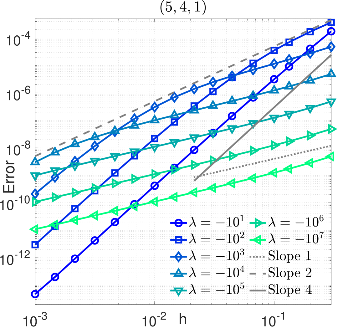
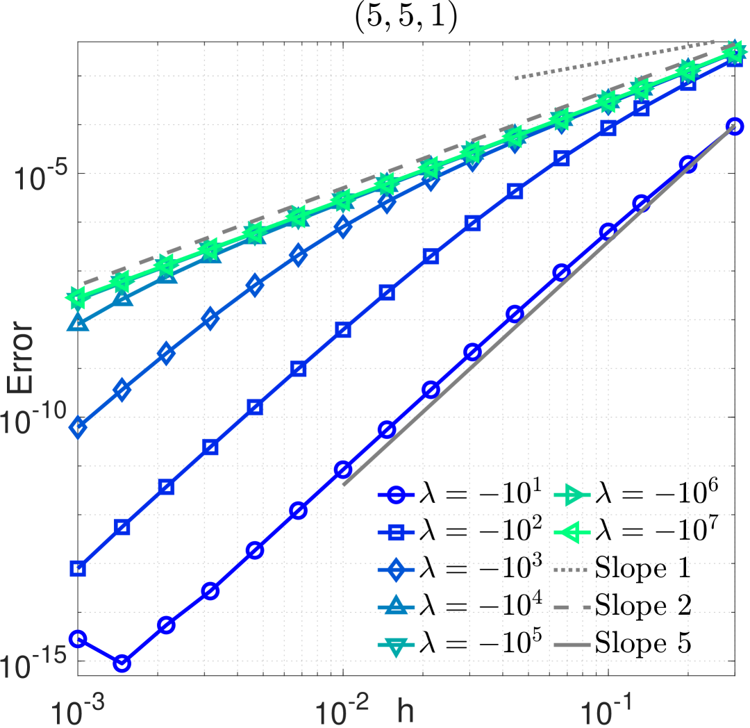
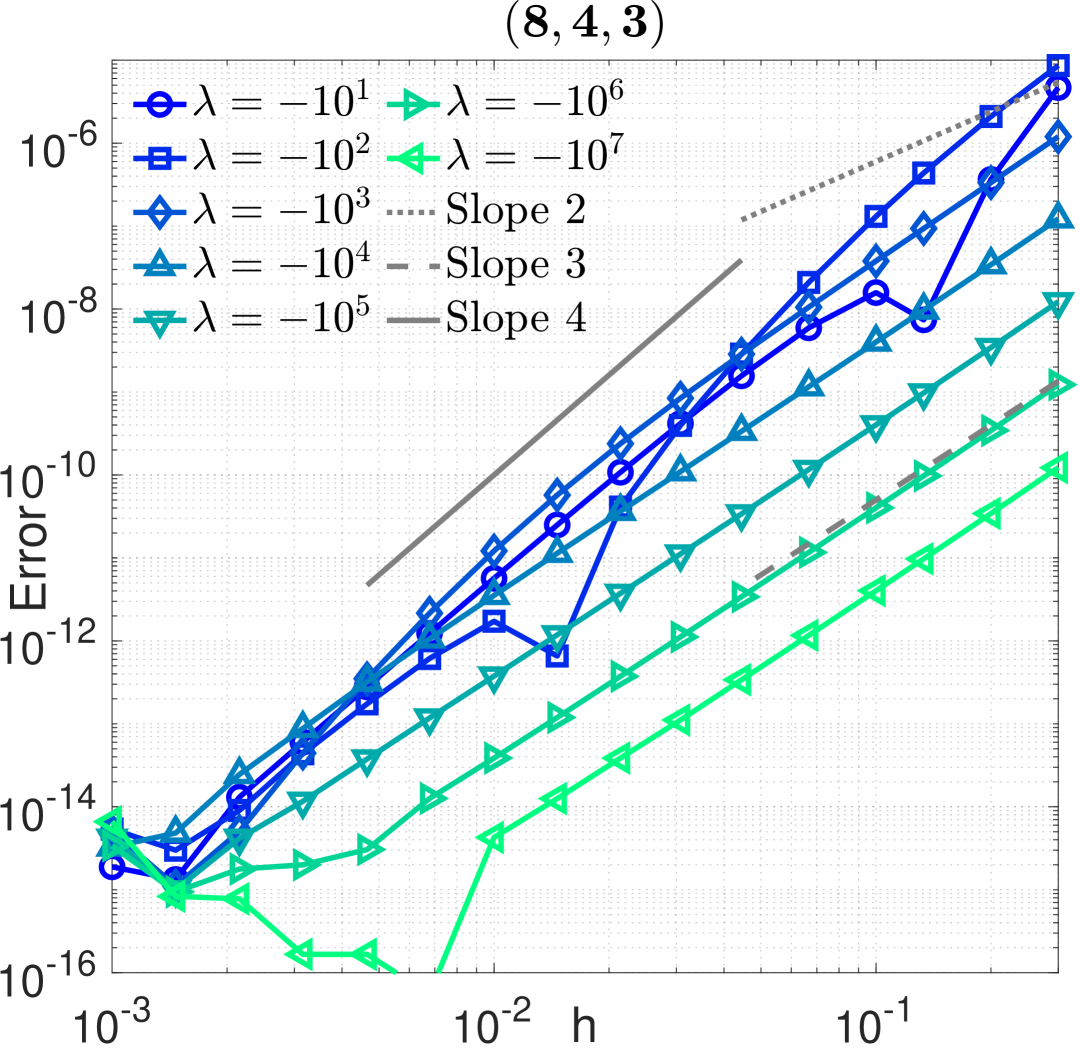
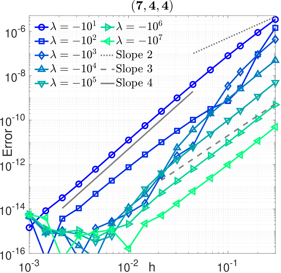
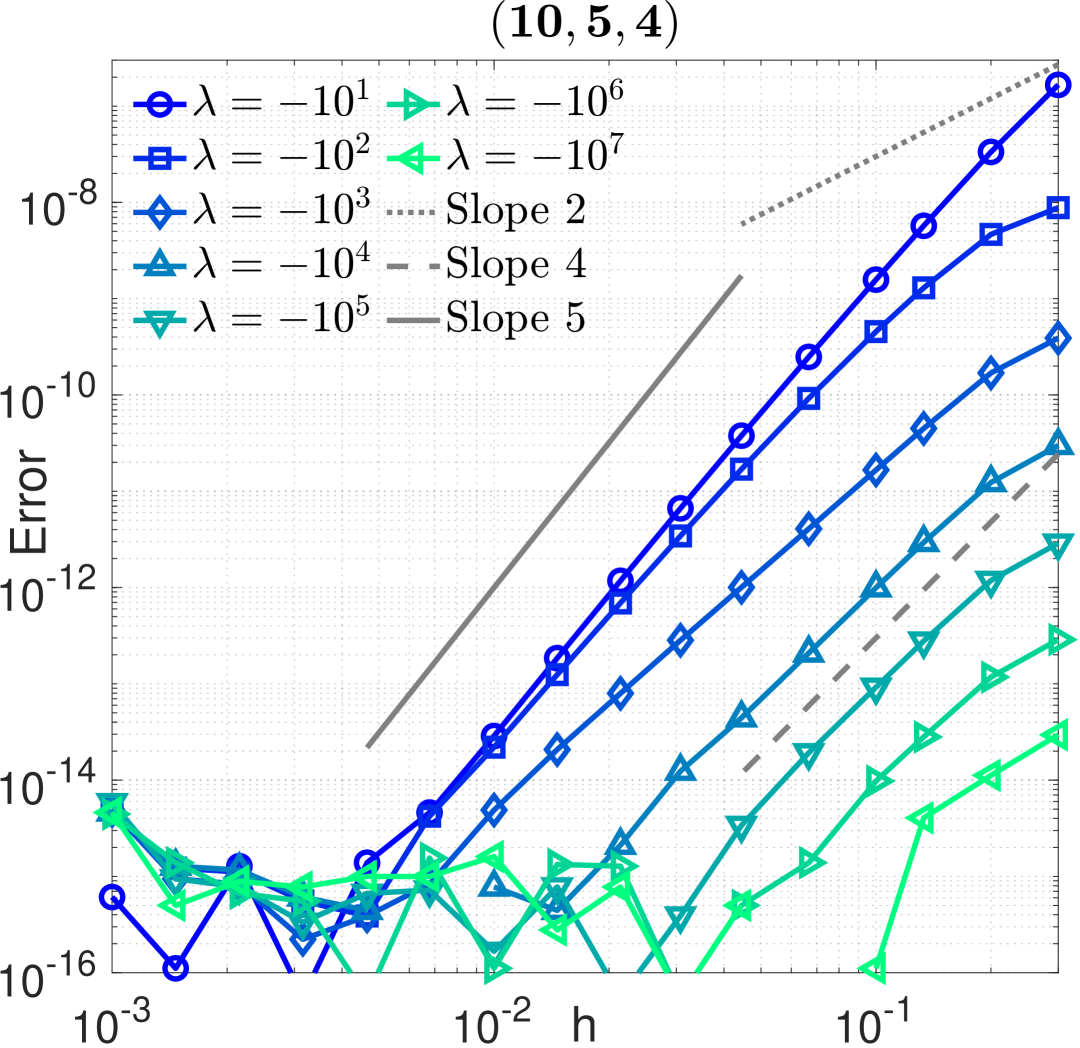
Figure 1: Error convergence of different methods for the semilinear Prothero–Robinson problem 84, shown for a family of choices of the stiffness parameter $\lambda$ (corresponding to the different curves). The top row shows classical reference methods, while the bottom row displays new methods with high semilinear orders. Of these, the left and the right panels show methods whose high semilinear orders satisfy $p_{\text{SL}}=p-1$, while the middle panel shows a 4th order method with $p_{\text{SL}}=p$. For notational efficiency, in all figures the methods from Table 2 are simply denoted by their triplet $(s,p,p_{\text{SL}})$.

Comparing different numerical methods, Fig. 1 shows the resulting error convergence curves (in classical double-logarithmic scale) for the problem 84 at final time $t=1.2$, using the stiffness parameter choices $\lambda=-10^{\nu}$ with $\nu\in\{1,\dots,7\}$. The bottom row of panels shows new methods with semilinear order $p_{\text{SL}}=p-1$ (left for $p=4$ and right for $p=5$) or $p_{\text{SL}}=p$ (middle for $p=4$). As discussed in Section 4, the two ESDIRK methods (8,4,3) and (10,5,4) are recommended for practical usage, while the EDIRK-(7,4,4) method is shown here to highlight the impact of $p_{\text{SL}}=p$.

The top row displays reference methods that satisfy the classical order conditions up to the respective orders ($p=4$ for left and middle, and $p=5$ on the right), but not any of the (other) semilinear order conditions. These top row results show that the reference methods (i) converge at their formal order $p$ in the non-stiff resolved regime ($\lambda h\ll 1$) and they (ii) clearly exhibit order reduction in the stiff regime ($\lambda h\gg 1$), reducing to first order. Furthermore, (iii) the family of error curves, parameterized by $\lambda$, lies uniformly below a line of slope 2, matching the B-convergence order indicated by the theory, i.e., the error estimate Theorem 5.

In contrast, the new methods, which satisfy the semilinear order conditions, do not exhibit the characteristic order-reduction L-shape that the classical methods shown around $\lambda h\approx 1$. In particular, for sufficiently small time step values, the new methods are notably more accurate than the reference schemes. At the same time, consistent with the definition of B-convergence, the new methods do not necessarily yield a uniform convergence rate throughout all time step values. Instead, there is a line of slope $\min(p,p_{\text{SL}}+1)$ below which all error curves lie for time steps sufficiently small, independent of the stiffness parameter $\lambda$. In this test, all error curves stagnate around machine precision. All new methods yield accurate results, including the EDIRK-(7,4,4) method.

5.2 A semilinear advection equation

We now consider several partial differential equation (PDE) test problems. Consistent with much of the mathematical literature, we denote a PDE’s solution by $u$, time by $t$, and space by $x$ (respectively $x_{1}$, $x_{2}$ in two space dimensions). The time step remains denoted by $h$. As a first test, we augment the linear advection equation by a nonlinear reaction term [hundsdorfer2003numerical], resulting in the semilinear problem

$$u_{t}+u_{x} =u^{2},\quad 0\leq x\leq 1,\quad 0\leq t\leq 5\;,$$ (85)

$$u(x,0) =u_{0}(x)\;,$$

$$u(0,t) =g_{0}(t)\;.$$

The inflow Dirichlet boundary conditions and the initial conditions are obtained from the analytical solution of 85, chosen as

$$u(x,t)=\frac{\sin^{2}(\pi(x-t))}{1-t\sin^{2}(\pi(x-t))}\;.$$

A key aspect in evaluating the effectiveness of time integration methods for such PDE problems is that a highly accurate spatial discretization technique is critical to effectively isolate the temporal error from the spatial approximation errors. To that end, a spatial discretization of at least order $p$ is used, with sufficiently high spatial resolution. For all studied time integration methods of orders up to $p=5$, a fifth-order finite difference approximation in space is employed via the methodology denoted as (4, 4, 6 - 6 - 4, 4, 4) in [carpenter1993stability], namely: approximate $u_{x}$ via sixth-order central differences in the domain’s interior, while using fourth-order one-sided finite differences near the boundary. This approach guarantees stability by ensuring that the spectrum of the resulting method-of-lines (MOL) matrix confined to the left-half complex plane.

As the theory in Section 3 allows for any inner-product-norm, we measure all spatial errors in a scaled $\ell^{2}$-norm which approximates the $L^{2}$-norm in space. Namely, if $y\in\mathbb{R}^{N}$ with values of $y_{j}$ on an equispaced grid, then $\left\lVert y\right\rVert_{2}^{2}=\frac{1}{N}\sum_{j=1}^{N}y_{j}^{2}$ (for Chebyshev grids in Section 5.3 there are additional weights in the summation). Norms involving the PDE solution use values of $u$ evaluated at the discrete grid points.

To ensure that spatial errors are negligible, we use 2048 spatial grid points which for the advection example yields a semi-discretization spatial error of $2.0\times 10^{-13}$. The spatial error is estimated by computing a reference solution to the method-of-lines (MOL) ODE via MATLAB’s ode45 with $\texttt{AbsTol}=10^{-14}$ and $\texttt{RelTol}=10^{-12}$. All figures report the numerical error of the fully discrete solution $U(t_{\mathrm{f}})$ against the PDE solution evaluated on the grid, $u(\cdot,t_{\mathrm{f}})$. This error is controlled by

$$\|U(t_{\mathrm{f}})-u(\cdot,t_{\mathrm{f}})\|_{2}\leq\underbrace{\|U(t_{\mathrm{f}})-u^{\mathrm{MOL}}(t_{\mathrm{f}})\|_{2}}_{\leq Dh^{q}\textrm{ from \lx@cref{creftype~refnum}{thm:convergence}}}+\underbrace{\|u^{\mathrm{MOL}}(t_{\mathrm{f}})-u(\cdot,t_{\mathrm{f}})\|_{2}}_{\leq 2\times 10^{-13}},$$ (86)

where $u^{\mathrm{MOL}}(t)\in\mathbb{R}^{N}$ is the (exact) MOL solution. In the subsequent numerical tests of temporal errors, error curves then tend to stagnate at that semi-discretization error value (which for the advection example is ${\sim}10^{-13}$). In turn, for errors above this value, the theory in Section 3 controls the fully discrete error with respect to the MOL solution; and thus the new methods are expected to converge at their full order $p$. The same error bound (86) holds below albeit with slightly different values for the spatial error.

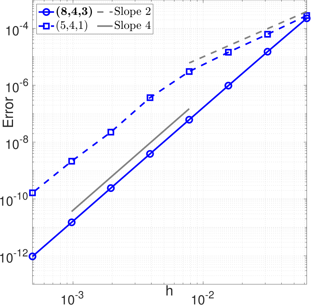
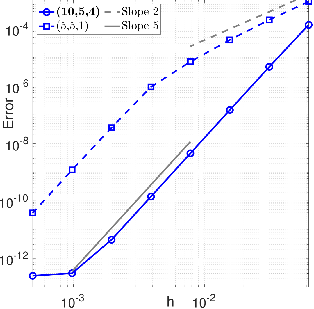
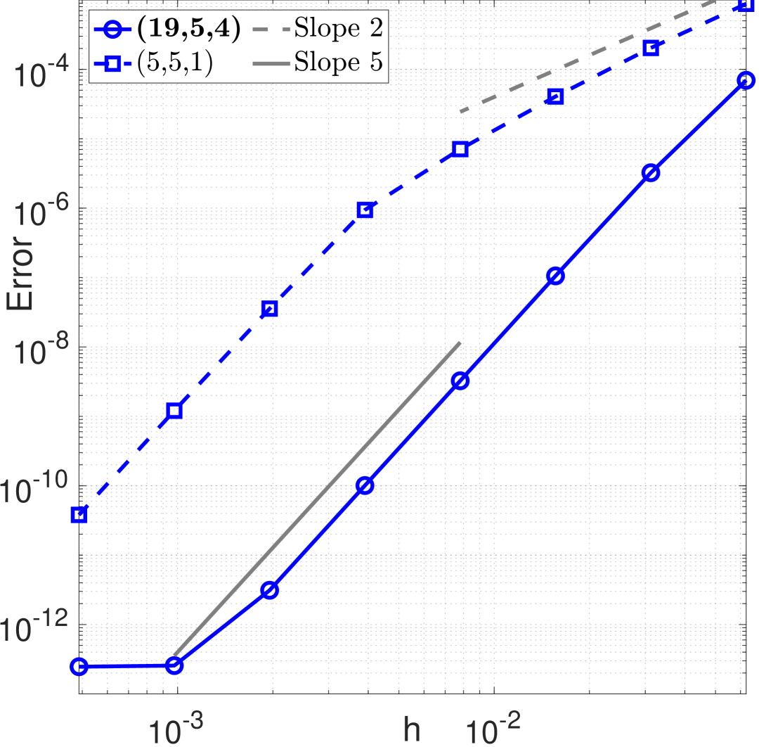
Figure 2: Error convergence (scaled $\ell^{2}$-norm) for the semilinear advection equation 85. In each panel a $p$-th order method satisfying the semilinear order conditions up to $p_{\text{SL}}=p-1$ is compared against a classical reference method of the same order $p$ but with $p_{\text{SL}}=1$. The new methods consistently exhibit the convergence orders established by the semilinear theory.

Figure 2 shows the convergence curves of the temporal errors, comparing the new methods against classical reference methods, with all errors evaluated at final time $t=0.5$. In each panel we can see that the reference method does exhibit order reduction, reducing to a slope of 2 (cf. [rosales2024spatial]) in the stiff regime. In contrast, the new methods with high semilinear order $p_{\text{SL}}\geq p-1$ converge at the full order $p$, up until spatial approximation errors dominate. In fact, convergence tests were conducted for all available methods, including those with $p_{\text{SL}}=p$. The outcome is that $p_{\text{SL}}=p-1$ generally suffices to achieve the full convergence order $p$; hence only such methods are displayed here.

In line with Section 4, the two ESDIRK methods (8,4,3) and (10,5,4), presented here, are recommended for practical usage. In addition, the EDIRK-(19,5,4) method is shown here as an example of a method of interest for PDE problems, which can be constructed via extrapolation. Due to its excessive number of stages, this method is largely of conceptual interest; however, the numerical results reveal that it exhibits acceptable accuracy, being a bit more accurate than the ESDIRK-(10,5,4) method.

5.3 Allen–Cahn equation in two space dimensions

We now study the numerical methods on a problem in two spatial dimensions. We consider the Allen–Cahn equation

$$u_{t}=\alpha\nabla^{2}u+\beta(u-u^{3})+f(x_{1},x_{2},t),\quad\ 0\leq x_{1},x_{2}\leq 1,\quad 0\leq t\leq 0.5\;,$$ (87)

with the parameter choices $\alpha=0.1$ and $\beta=3$. The initial conditions, the time-dependent Dirichlet boundary conditions, and the source term $f(x_{1},x_{2},t)$ are such that the manufactured solution is $u(x_{1},x_{2},t)=2+\sin(2\pi(x_{1}-t))\cos(3\pi(x_{2}-t))$. Equation 87 is a nonlinear reaction-diffusion PDE used for example in multiple types of multiphase state systems. Because its differential operator is linear, similar convergence behavior of the various time-stepping methods as found in Section 5.2 may be expected.

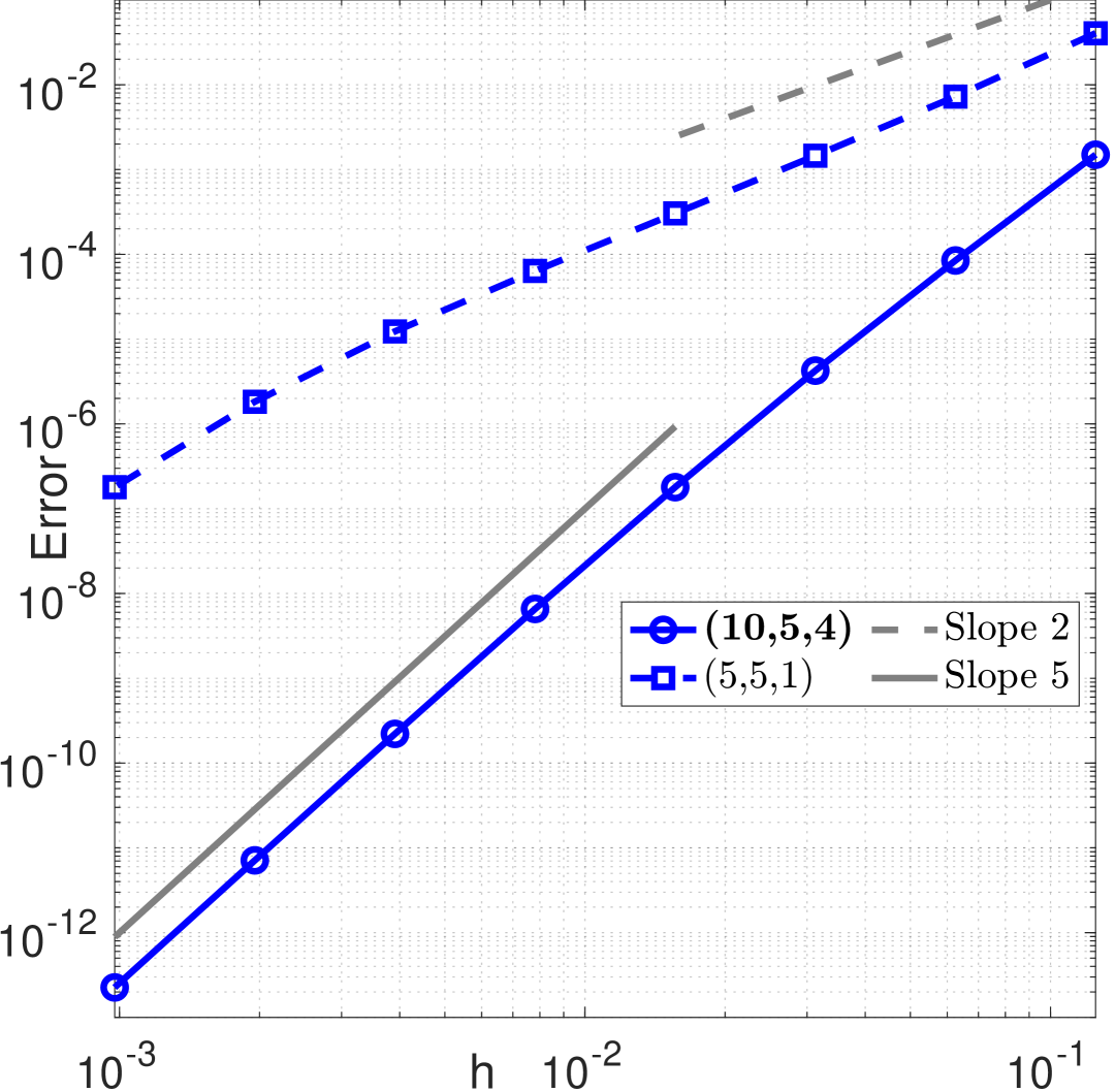
Figure 3: Error convergence (scaled $\ell^{2}$-norm) for the Allen–Cahn equation 87 in two space dimensions. Left panel: Middle: 4th-order methods with $p_{\text{SL}}=1$ and $p_{\text{SL}}=p-1$. Right: 5th-order methods with $p_{\text{SL}}=1$ and $p_{\text{SL}}=p-1$. The methods exhibit the convergence orders established by the semilinear theory.

The spatial approximation in conducted via spectral methods on a 2D tensor product grid, using $25$ Chebyshev grid points in each dimension. This results in a spatial approximation error of $6.04\times 10^{-15}$ in the scaled $\ell^{2}$-norm.

We now time-step the resulting systems until $t=0.5$ via the various methods, and compute the errors in the scaled $\ell^{2}$-norm in space. Figure 3 displays the convergence results of the new methods in comparison against classical methods from the literature. In line with [rosales2024spatial], those classical methods exhibit a convergence rate of about 2, despite having formal orders of 4 and above. In contrast, the new methods with $p_{\text{SL}}=p-1$ exhibit convergence rates (very close to) $p$ for all tested methods, confirming that the conditions and methods presented herein can effectively alleviate order reduction also for problems in higher spatial dimensions.

5.4 Viscous Burgers’ equation

As a stiff nonlinear PDE problem, we study the viscous Burgers’ equation,

$$u_{t}+uu_{x}=\nu u_{xx}+f\ \ \text{for}\ (x,t)\in(0,1)\times(0,1],\quad u=g\ \ \text{on}\ \{0,1\}\times(0,1]\;,$$ (88)

with a viscosity constant $\nu=0.1$, which is large enough to ensure that the computational grid used accurately captures the spatial scales of the solution, but small enough to ensure that the nonlinear term is relevant for the observed approximation errors. The initial condition $u(x,0)$ and Dirichlet boundary values are chosen to match the exact solution $u(x,t)=\cos(2+10t)\sin(0.2+20x)$. A uniform grid is used for the spatial discretization, with both spatial derivatives approximated using sixth-order finite centered differences, on a grid of $10^{3}$ cells. This yields a spatial error of $2.87\times 10^{-13}$ (found in the same way as in the above tests), thus ensuring that the temporal error is isolated in the convergence study. For time integration, we employ our proposed methods alongside classical approaches and calculate the errors at a final time $t=1$ using the scaled $\ell^{2}$-norm in space.

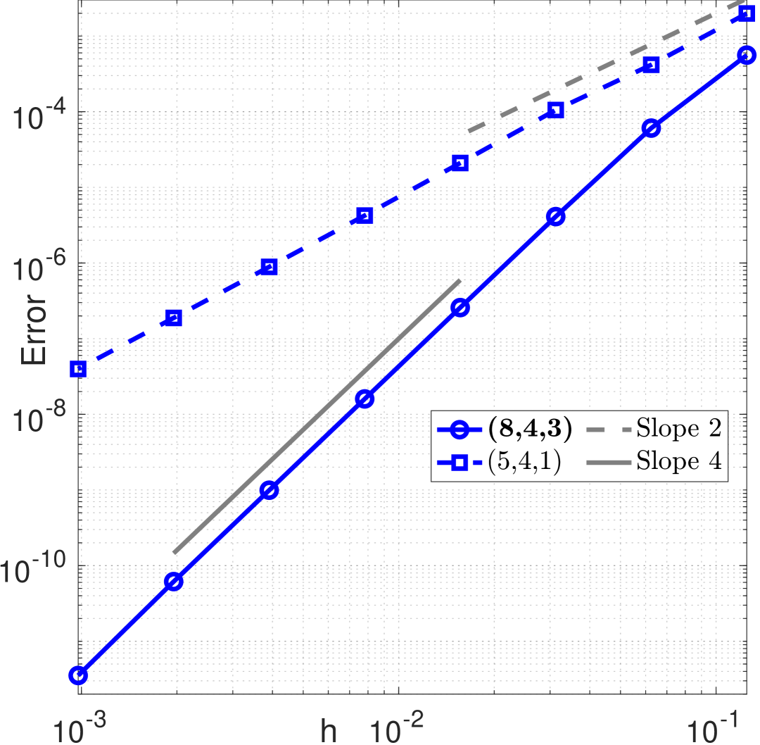
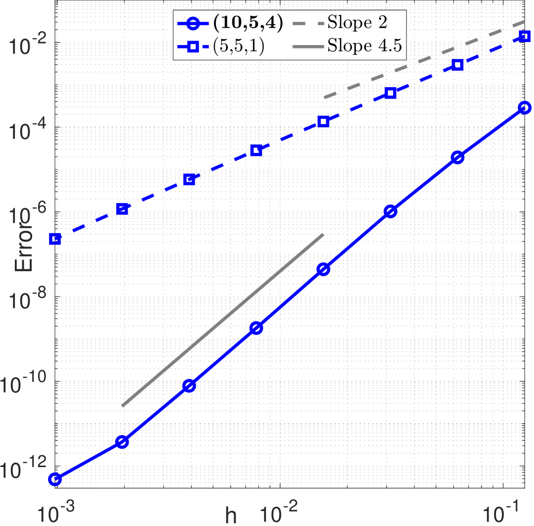
Figure 4: Error convergence (scaled $\ell^{2}$-norm) for the viscous Burgers’ equation 88. Left panel: 4th-order methods with different semilinear orders, in which the new method with high semilinear order exhibits convergence at order $p$. Right panel: 5th-order methods with different semilinear orders. Here the new method exhibits convergence order 4.5, which is less than $p$ but significantly better than the order 2 of the reference method.

Figure 4 shows the error convergence results over the range $10^{-3}\leq h\leq 10^{-1}$, which represents natural time step choices for the given test problem and spatial discretization. Unlike the previous PDE tests, the problem here is not covered by the theory in Section 3 because we are not in the regime where the time step $h$ is small relative to the Lipschitz constant of the nonlinear term, which scales like the number of spatial grid points.

The results illustrate that all classical methods converge with an order of $2$ and hence exhibit order reduction. The new methods, however, converge at orders 4.0 for the ESDIRK-(8,4,3) and 4.5 for the ESDIRK-(10,5,4) methods respectively. These observations are consistent with related numerical results [biswas2023design], revealing that weak stage order (in [biswas2023design]) and/or semilinear order conditions can manifest in significant accuracy benefits, even for test cases that lie outside the convergence theory (albeit not necessarily at the full order $p$).

5.5 Van der Pol equation

As an example of a stiff, truly nonlinear ODE problem not of the semilinear form 1, we consider the Van der Pol test problem as defined in [hairer1996solving, Chapter VI.3, p. 406]

$$\begin{split}y^{\prime}_{1}&=y_{2}\;,\\ \epsilon y^{\prime}_{2}&=(1-y_{1}^{2})y_{2}-y_{1}\;,\end{split}$$ (89)

with $t\in(0,0.5]$. The initial condition is given by

$$(y_{1}(0),y_{2}(0))=\left(2,-\tfrac{2}{3}+\tfrac{10}{81}\epsilon-\tfrac{292}{2187}\epsilon^{2}-\tfrac{1814}{19683}\epsilon^{3}\right).$$

We consider the values $\epsilon=10^{-3}$, representing a mildly stiff regime, and $\epsilon=10^{-6}$, corresponding to a strongly stiff regime.

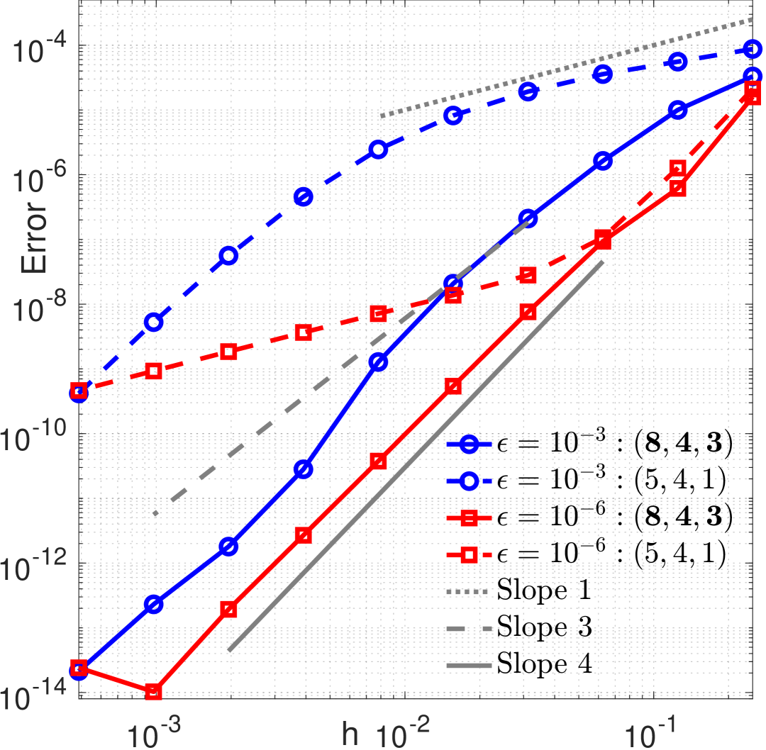
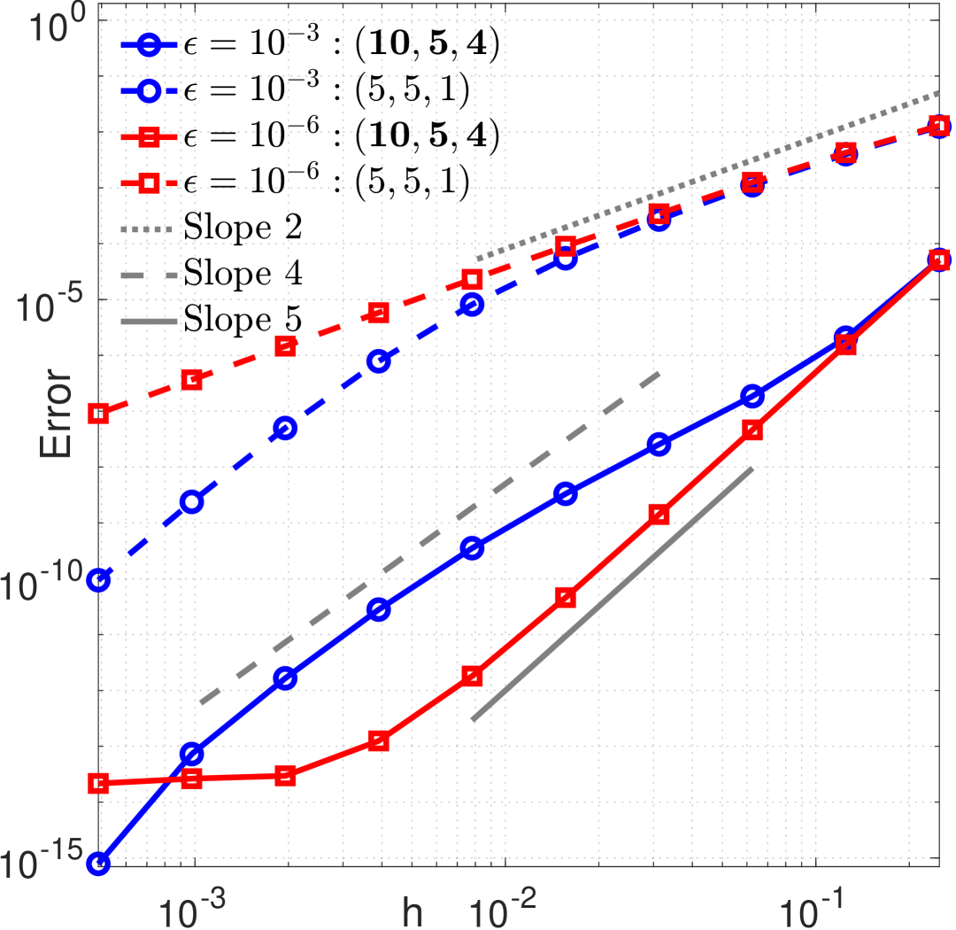
Figure 5: Error convergence for the Van der Pol equation 89. Left panel: 4th-order methods with different semilinear orders. Right panel: 5th-order methods with different semilinear orders. Even though this test lies fully outside the semilinear theory, the new methods with high semilinear order nevertheless alleviate order reduction effects.

The reference solution at the final time is computed using MATLAB’s ode45 solver with $\texttt{AbsTol}=\texttt{RelTol}=5\times 10^{-14}$. Figure 5 shows the numerical convergence rates of solutions obtained through our proposed methods and classical methods. As the problem lies fully outside the class of semilinear problems, our proposed methods are not guaranteed to eliminate order reduction; and the numerical results confirm that in fact, order reduction effects are still present. At the same time, the new methods do consistently enhance the convergence rates relative to the reference schemes, resulting in significantly smaller approximation errors.

The numerical results also reveal an interesting impact of the stiffness parameter $\epsilon$. In the mildly stiff case $\epsilon=10^{-3}$, transitions in the slopes of the error curves are observable across the tested $h$-range, characteristic for order reduction. In contrast, in the strongly stiff case $\epsilon=10^{-6}$, the reference schemes exhibit convergence orders 1 (the SDIRK-(5,4,1) method for $10^{-3.5}<h<10^{-1.5}$) or 2 (the SDIRK-(5,5,1) method); while the tested new methods with high semilinear order do exhibit convergence orders $p$. This highlights that the new methods may, for certain stiff nonlinear problems, perform even better than the theory would predict.

6 Conclusion

In this work, we have developed a rigorous error and convergence analysis for Runge–Kutta methods applied to semilinear ODEs where the linear term can be arbitrarily stiff. For this class of problems, classical analysis can only provide error estimates in the asymptotic limit, i.e., when the time step is small relative to the two-sided Lipschitz constant of the right-hand side. For implicit methods, however, we typically want to take time steps well outside the asymptotic regime—which can cause order reduction. In contrast to the classical analysis, the B-convergence results established in this work hold uniformly with respect to stiffness.

The approach to deriving semilinear order conditions presented here adapts a unique recursion originally proposed by Albrecht [albrecht1987new, albrecht1996runge]. Up to order three in the LTE, the semilinear order conditions correspond to conditions already known for linear problems [biswas2022algebraic]. This structural insight in particular rationalizes why existing methods with high weak stage order manage to mitigate order reduction on problems outside what previous theory could predict. Starting at fourth order terms in the LTE, new order conditions arise, i.e., semilinear order strictly goes beyond weak stage order. All of the semilinear order conditions have been established to be in one-to-one correspondence with rooted trees.

Based on the semilinear order framework, four new Runge–Kutta methods have been proposed that satisfy the semilinear order conditions and possess other desirable properties, as follows. For order four and five, the two methods ESDIRK-(8,4,3) and ESDIRK-(10,5,4) are recommended to be used in practical applications where order reduction could be a concern, like problems of the type of those presented in Section 5. Both methods are optimized for stability and accuracy—as demonstrated by the numerical results in Section 5.

The other two methods, EDIRK-(7,4,4) and EDIRK-(19,5,4), are less optimized and thus are primarily of theoretical interest. Notably, they highlight that methods with stage order 1 can achieve semilinear order 4.

Due to its structural relation to the theory developed in [luan2013exponential], the here presented semilinear order theory brings stiff Runge–Kutta order conditions in line with existing theory for exponential integrators. A key theoretical question open to future investigation is whether a single, unifying theory for exponential and Runge–Kutta order conditions can be established. Another intriguing open question is whether a B-series version of Albrecht’s order conditions can be provided.

Because the implicit Runge–Kutta framework considered herein (generally) requires nonlinear solves, a natural goal for future work is to extend the framework to other methods that may get away with less demanding solves, such as Rosenbrock methods or implicit-explicit Runge–Kutta methods. Finally, in the context of stiff problems, the limit of differential-algebraic equations (DAEs) is also a natural point of study. As the results in Fig. 5 indicate, the presented new schemes may indeed perform well also for problems close to the DAE limit.