Shapes and orientations of massive halos
in the statistically anisotropic universe

Abstract

We investigate how statistical anisotropy (SA) in matter distributions affects the shapes and orientations of cluster-sized halos, using cosmological $N$-body simulations that incorporate SA. While the three-dimensional halo shape parameters show little dependence on SA, we find that halo orientations are significantly influenced, with halos tending to align either perpendicular or parallel to the SA direction. This SA-induced alignment becomes more prominent for more massive halos. Our findings suggest that observational measurements of projected halo shapes, such as those derived from galaxy cluster-galaxy lensing, could provide a novel probe of SA in the universe.

I introduction

Statistical isotropy, also referred to as global isotropy, is a foundational conjecture in cosmology. It implies that the statistical properties of density fluctuations are independent of direction. While this conjecture is supported by various observations, such as the cosmic microwave background (CMB) and galaxy distributions, theoretical models involving vector fields naturally lead to its violation. Thus, the possibility of broken isotropy—known as statistical anisotropy (SA)—in cosmological matter distributions remains open.

SA can arise from anisotropic sources such as vector fields, which could appear in anisotropic inflationary scenarios (see [1, 2, 3] for review), vector dark matter [4, 5, 6], and vector dark energy models [7]. In particular, inflationary models with gauge fields, including the anisotropic inflation model, have been extensively discussed, e.g., in the context of axion cosmology based on the string theory, primordial magnetogenesis, and so on. Thus, exploring the SA may indirectly provide a means to probe the matter contents such as gauge fields in the early universe.

The quadrupolar type of SA, the leading-order term [8], is characterized by only one magnitude parameter $g_{*}$, which has been constrained by the CMB measurements of Planck satellite observations [9, 10, 11], yielding $|g_{*}|=\mathcal{O}(10^{-2})$. Additional efforts have been made to constrain SA using galaxy clustering measurements [12, 13] (see Refs. [14, 15, 16] for the practical analysis techniques using the polypolar spherical harmonic basis). Recently, Ref. [17] performed cosmological $N$-body simulations incorporating quadrupolar SA, and showed that SA induces anisotropic halo bias in the quadrupole moments of galaxy two-point statistics. Including this newly identified effect in the analysis enables more accurate constraints on $g_{*}$ beyond linear theory from galaxy clustering.

Since SA introduces a preferred direction in the initial conditions of matter distributions, and halo formation traces the underlying matter distribution, it is reasonable to expect that halo shapes and orientations may be altered and become somewhat anisotropic in the statistically anisotropic universe. Observationally, the projected shapes of massive halos have been studied mainly via galaxy cluster-galaxy lensing. For example, Ref. [18] measured the distribution of the projected ellipticity of massive halos using galaxy cluster-galaxy lensing signals and found consistency with predictions from cosmological simulations by Ref. [19]. Ref. [20] obtained the mean ellipticity of galaxy clusters using distributions of member galaxies as well as weak lensing. If SA affects halo shapes and/or orientations, the observable quantities, such as the projected halo ellipticity, would also exhibit systematic directional features, which could be detected through gravitational lensing observations. In such a case, comparisons between predictions from cosmological simulations with SA and observations of projected ellipticities could serve as a means to constrain $g_{*}$.

While Ref. [17] focused on SA-induced halo bias, in this work, we investigate how SA affects the shapes and orientations of cluster-sized halos at $z=0$ using cosmological simulations [19, 21, 22], with the aim of exploring their potential as a new probe of SA. We find that the three-dimensional shape parameters [21] show surprisingly little dependence on the quadrupolar SA parameter $g_{*}$. In contrast, halo orientations are more strongly influenced by SA. Specifically, halos tend to increasingly align perpendicular to the SA-preferred direction for positively larger $g_{*}$, and parallel for negatively larger $g_{*}$. We also find that this alignment effect becomes more pronounced for more massive halos. Given that halo structures encode information about the underlying matter field, studying their response to SA offers a complementary approach to existing clustering-based analyses. This motivates our investigation of halo shapes and orientations as potential observational tracers of SA.

The rest of this paper is organized as follows. In Sec. II, we describe the cosmological $N$-body simulations incorporating SA, the halo catalogs used in this work, and the measured quantities related to the halo shapes. Sec. III presents our results on the halo shapes and orientations. We summarize and conclude in Sec. IV.

II setup

In this section, we briefly describe how to quantify the SA and how to obtain the halo catalog in the simulated universe with the SA. Then, we introduce the quantities measured in simulations that characterize the shape and orientation of identified halos.

II.1 Cosmological $N$-body simulations with SA

We follow Ref. [17] to perform the cosmological $N$-body simulations with SA. First let us introduce the SA in the matter distributions. In our study, we consider the quadrupolar type of SA, and the power spectrum of initial linear matter overdensity fields is written by $\left\langle\delta_{\mathrm{m}}(\mathbf{k}_{1})\delta_{\mathrm{m}}(\mathbf{k}_{2})\right\rangle=(2\pi)^{3}\delta^{(3)}(\mathbf{k}_{1}+\mathbf{k}_{2})\mathit{P}_{\mathrm{m}}(\mathbf{k}_{1})$ with

$$\mathit{P}_{\mathrm{m}}(\mathbf{k})=\left[1+\frac{2}{3}g_{*}\mathcal{L}_{2}(\mu)\right]\bar{P}_{\mathrm{m}}(k),$$ (1)

where $g_{*}$ descibes the magnitude of SA, $\bar{P}_{\mathrm{m}}(k)$ means the isotoropic component of the matter power spectrum, $\mathcal{L}_{2}\equiv\frac{1}{2}(3\mu^{2}-1)$ with $\mu\equiv\hat{\mathbf{k}}\cdot\hat{\mathbf{d}}$ and $\hat{\mathbf{k}}\equiv\mathbf{k}/|\mathbf{k}|$, and $\hat{\mathbf{d}}$ is the directions related to SA.

SA in matter distributions is incorporated by using Eq. (1) when generating the initial conditions (ICs), where the direction of SA is set to $\hat{\mathbf{d}}=(0,~0,~1)$. We use the Boltzmann code CAMB [23] to compute the isotropic linear matter power spectrum $\bar{P}_{\mathrm{m}}(k)$ in Eq. (1) at the initial redshift $z_{\rm ini}=31$. Based on the computed $\bar{P}_{\mathrm{m}}(k)$, ICs are generated using the second-order Lagrangian perturbation theory [24, 25, 26]. We input the ICs into the cosmological $N$-body solver Gadget-2 [27, 28] to follow the evolution of matter distributions in statistically anisotropic universes.

Table 1: Summary of the simulation settings: $N_{\rm part}$, $L_{\rm box}$, $m_{\rm part}$, and $g_{*}$ stand for the number of simulation particles, the size of the simulation box, the mass of a simulation particle, and the magnitude of the quadrupolar-type SA, respevtively

. run $N_{\rm part}$ $L_{\rm box}$ $[h^{-1}{\rm Gpc}]$ $m_{\rm part}$ $[h^{-1}M_{\odot}]$ $g_{*}$ L05 $512^{3}$ $0.5$ $8.16\times 10^{10}$ $0,~\pm 0.1,~\pm 1$ L2 $1024^{3}$ $2$ $6.53\times 10^{11}$ $0,~\pm 0.1,~\pm 0.5,~\pm 1$ L4 $1024^{3}$ $4$ $5.22\times 10^{12}$ $0,~\pm 0.1,~\pm 1$

Except for assuming Eq. (1) as the initial matter power spectrum, in the $N$-body simulation, we assume the standard flat-$\Lambda$ cold dark matter cosmology with the Planck’s best fit cosmlogical parameters as $\Omega_{\rm m0}=0.3156,~\Omega_{\Lambda 0}=0.6844,~H_{0}=100h=67.27~{\rm km~s^{-1}~{\rm Mpc}^{-1}},~n_{\rm s}=0.9645$ and $A_{\rm s}=2.2065\times 10^{-9}$ [29]. We perform three simulations characterized by the number of particles $N_{\rm part}$ and the box size $L_{\rm box}$, as summarized in Table 1. To study the $g_{*}$-dependence of halo properties, for each simulation we vary $g_{*}$ values as listed in the table. For each simulation setting, we conduct four realizations, resulting in a total of 68 realizations.

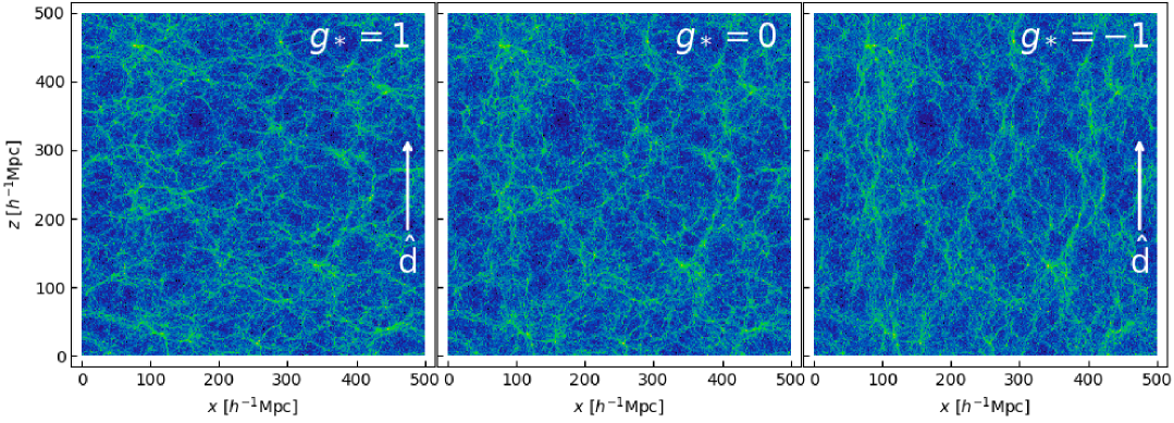
Figure 1: Visualizations of the matter distributions at the redshift $z=0$ in the $x$-$z$ plane, in the simulated universes with $g_{*}=+1$ (left), $0$ (middle), and $-1$ (right). Each panel shows a $50~h^{-1}{\rm Mpc}$-thick slice along the $y$-direction taken from the realization with the same initial random seed in the L05 run. The SA direction $\hat{\mathbf{d}}$ is shown in each panel.

To facilitate a visual understanding of the impact of $g_{*}$, Fig. 1 shows the matter distributions at $z=0$ in the $x$-$z$ plane for the simulated universes with $g_{*}=+1$ (left), $0$ (middle), and $-1$ (right). Each panel describes a $50~h^{-1}{\rm Mpc}$ thick slice along the $y$-direction taken from the realization with the same initial random seed in the L05 run. Compared to the middle panel with $g_{*}=0$ (i.e., the isotropic case), the matter distribution is elongated perpendicular to the SA direction $\hat{\mathbf{d}}$ for $g_{*}=+1$ (left), and along $\hat{\mathbf{d}}$ for $g_{*}=-1$ (right).

II.2 Halos as ellipsoids

To identify halos in the simulated matter distributions, we use the halo finder code Rockstar [30]. As the halo mass, we employ the mass within a region whose average density is 200 times the cosmological matter density, denoted as $M_{\rm 200b}$. Since measuring halo shapes requires a sufficient number of particles, we analyze only halos that contain more than approximately 200 particles. On the other hand, a larger simulation box is needed to obtain more massive halos due to their low abundance. Taking these factors into account, we use halos with masses of $\log_{10}[M_{\rm 200b}/(h^{-1}M_{\odot})]\in(13,~13.5]$, $(14,~14.5]$, and $(15,~15.5]$ from the L05, L2, and L4 runs, respectively.

To describe the shapes of halos, we regard the halos as ellipsoids characterized by three axes, $a$, $b$, and $c$ with $a\geq b\geq c$. Based on these three axes, we introduce normalized variables characterizing the halo shape [31, 21]

$$s:=\frac{c}{a},~q:=\frac{b}{a},~T:=\frac{a^{2}-b^{2}}{a^{2}-c^{2}}=\frac{1-q^{2}}{1-s^{2}},$$ (2)

where $s$ and $q$ are the smallest- and intermediate-to-largest axis ratios, respectively, and $T$ is the so-called triaxiality of halos. For these shape parameters, we directly use the values of $s$ and $q$ produced by Rockstar, which are measured using the weighted inertia tensor of halos [21].

As for the parameter characterizing the orientations of halos, we utilize the vector assigned for each halo in the Rockstar halo catalog, $\mathbf{A}=\left(A_{x},~A_{y},~A_{z}\right)$, which corresponds to the largest axis of the ellipsoid. To clearly show the $g_{*}$-dependence of the orientations of halos, we use the arranged vector with respect to the $z$-direction (i.e., the SA direction in this work) as

$$\mathbf{\hat{A}}=\left(\hat{A}_{x},~\hat{A}_{y},~\hat{A}_{z}\right)$$ (3)

$$=$$

so that the probability distribution functions (PDFs) of the orientations of halos is uniformly random in the isotropic universe. The normalization is performed to enable comparison of results across different halo mass ranges.

III results

In this section, we present our results on the shapes and orientations of halos at $z=0$ in the statistically anisotropic universe.

III.1 The halo shapes

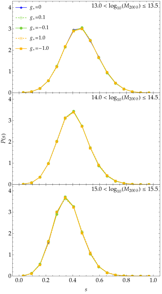
Figure 2: PDF of $s$, $P(s)$, for the three halo mass ranges of $\log_{10}[M_{\rm 200b}/(h^{-1}M_{\odot})]\in(13,~13.5],~(14,~14.5]$ and $(15,~15.5]$ obtained from the L05, L2, and L4 runs, respectively. Each color line shows the result for $g_{*}=0$ (blue), $\pm 0.1$ (green) and $\pm 1.0$ (orange), and the dashed (solid) lines are for the cases with the positive (negative) sign. We note that all the five curves almost overlap.

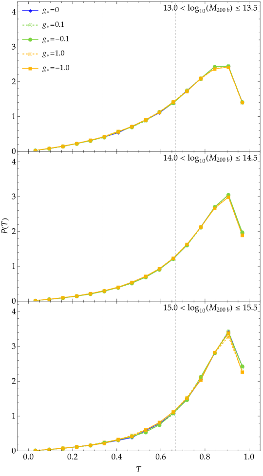
Figure 3: Same as Fig. 2 but for the PDF of $T$. The vertical dashed line in each panel indicates the boundaries between halo shape categories: “oblate” for $T<1/3$, “triaxial” for $1/3<T<2/3$, and “prolate” for $2/3<T<1$. Similarly to the Fig. 2, all the five curves almost overlap.

We investigate the effect of SA on the shapes of halos, and in particular, we focus on the parameters $s$ and $T$, which respectively represent the smallest-to-largest axis ratio and triaxiality of the halo as an ellipsoid. Fig. 2 shows the $g_{*}$-dependence of the PDFs of $s$, $P(s)$, for the three halo mass ranges of $\log_{10}[M_{\rm 200b}/(h^{-1}M_{\odot})]\in(13,~13.5],~(14,~14.5]$ and $(15,~15.5]$ obtained from the L05, L2, and L4 runs, respectively. Each color line in this figure shows the result for $g_{*}=0$ (blue), $\pm 0.1$ (green) and $\pm 1.0$ (orange) (dashed line for the positive sign, and solid line for the negative sign). The error bars represent the standard error across the four realizations for each value of $g_{*}$ within a given run (i.e., fixed $L_{\rm box}$ and $N_{\rm part}$). We note that all the PDFs in this paper are normalized to integrate into one over the entire domain. Though we are focusing on the relatively massive halos, the shape of the PDF itself seems to be consistent with the previous studies in the statistically isotropic universe (see, e.g., Ref. [21]), e.g., the peak of $P(s)$ is around $s=0.4$, and a weak mass dependence of the peak position is also visible in this figure. Then, as for the $g_{*}$-dependence, from this figure, even in the statistically anisotropic universe with the $g_{*}$ values much larger than those currently favored by the CMB observations, it is hard to find the difference from the isotropic one. We also observe a similarly negligible deviation from the isotropic case in the PDFs of the triaxiality, $T$, $P(T)$, shown in Fig. 3. Thus, we conclude that for the cluster-sized massive halos the SA effect on the shape is negligible. We expect that the above result on the shapes can be understood as follows. As discussed in Refs. [16, 17], the power spectrum of initial linear matter overdensity fields given by Eq. (1) can be rewritten as

$$\mathit{P}_{\mathrm{m}}(\mathbf{k})=\left[1+\mathcal{G}_{ij}\hat{k}_{i}\hat{k}_{j}\right]\bar{P}_{\mathrm{m}}(k)~,$$ (4)

with a global traceless tensor field:

$$\mathcal{G}_{ij}\equiv g_{*}\left(\hat{d}_{i}\hat{d}_{j}-\frac{1}{3}\delta_{ij}\right).$$ (5)

This means that, in our setup, the SA can be understood as the coupling between the matter density field and the global tensor field, and hence the SA effect is considered to be global. Thus, such a global effect is not expected to have much impact on the halo shape, which would highly depend on nonlinear dynamics in the halo-sized local region.

III.2 The halo orientations

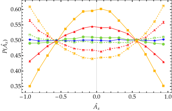
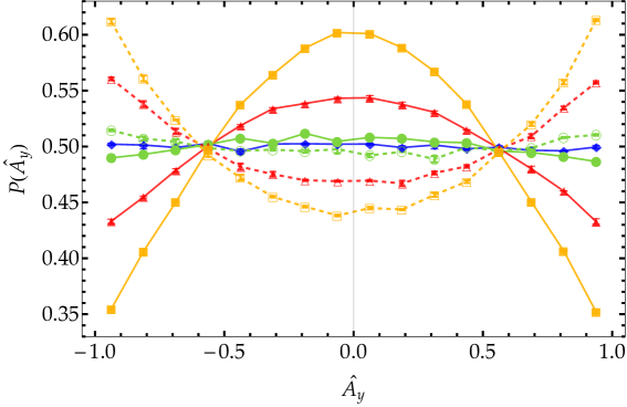
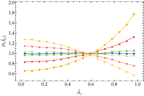
Figure 4: PDFs of $\hat{A}_{x},~\hat{A}_{y}$ and $\hat{A}_{z}$, i.e., the halo orientations, for the halos with masses of $14<\log_{10}[M_{\rm 200b}/(h^{-1}M_{\odot})]\leq 14.5$ from the L2 run. Each color line shows the result for $g_{*}=0$ (blue), $\pm 0.1$ (green), $\pm 0.5$ (red) and $\pm 1.0$ (orange), and the dashed (solid) lines are for the cases with the positive (negative) sign.

As we have discussed in the previous subsection, we found that the SA effect on the halo shape is negligible. To explore whether there are any halo properties that are affected by the SA, we next examine the orientation of the halo as an ellipsoid. In Fig. 4, we show the PDFs of the components of the vector $\mathbf{\hat{A}}$, which characterizes the orientation of the largest axis of each halo, and here we use the halos with masses in the range of $14<\log_{10}[M_{\rm 200b}/(h^{-1}M_{\odot})]\leq 14.5$, taken from the L2 run only. Each color line shows the result for $g_{*}=0$ (blue), $\pm 0.1$ (green), $\pm 0.5$ (red) and $\pm 1.0$ (orange), and the dashed (solid) lines are for the cases with the positive (negative) sign. Note that $\hat{A}_{x}$ and $\hat{A}_{y}$ take values in the range $[-1,~1]$, while $\hat{A}_{z}$ takes values in the range $[0,~1]$ due to our setup described in Eq. (3).

In the isotropic case, i.e., $g_{*}=0$, $P(\hat{A}_{x}),~P(\hat{A}_{y})$ and $P(\hat{A}_{z})$ are completely flat, indicating that the distribution of the orientations of halos is uniformly random.. Unlike the shape parameters shown in Figs. 2 and 3, the halo orientations exhibit a clear dependence on $g_{*}$. As $g_{*}$ increases positively, both $P(\hat{A}_{x})$ and $P(\hat{A}_{y})$ exhibit increasing curvature, developing deeper minima at $\hat{A}_{x}=0$ and $\hat{A}_{y}=0$, and more pronounced maxima at $\hat{A}_{x}=\pm 1$ and $\hat{A}_{y}=\pm 1$, respectively. In contrast, $P(\hat{A}_{z})$ shows the opposite trend, peaking at $\hat{A}_{z}=0$ and reaching a minimum at $\hat{A}_{z}=1$. These behaviors indicate that, for larger positive values of $g_{*}$, halos as ellipsoids tend to align parallel to either the $x$-axis or the $y$-axis.

Conversely, as $g_{*}$ decreases (i.e., becomes more negative), $P(\hat{A}_{z})$ becomes a steeper increasing function of $\hat{A}_{z}$, exhibiting a higher peak at $\hat{A}_{z}=1$ and a lower minimum at $\hat{A}_{z}=0$. Correspondingly, $P(\hat{A}_{x})$ and $P(\hat{A}_{y})$ show the opposite behavior, peaking at $\hat{A}_{x}=0$ and $\hat{A}_{y}=0$ and reaching minima at $\hat{A}_{x}=\pm 1$ and $\hat{A}_{y}=\pm 1$, respectively. This means that, for negative values of $g_{*}$, halos tend to align parallel to the $z$-axis.

In summary, halo orientations tend to increasingly align perpendicular to $\hat{\mathbf{d}}$ for larger positive values of $g_{*}$, and parallel to $\hat{\mathbf{d}}$ for lower negative values. This trend is consistent with the visualizations of matter distributions on large scales presented in Fig. 1. As discussed in the previous subsection, the SA in our setup can be considered as the effect of the global tensor field, and then the alignment of the halos can be affected by the global structure (see, e.g., Ref. [16]).

Let us mention a few behaviors of PDFs observed in Fig. 4, that are related to the symmetry in our setup. First, $P(\hat{A}_{x})$ and $P(\hat{A}_{y})$ are nearly identical. This is because the $x$- and $y$-axes are both perpendicular to the SA direction $\hat{\mathbf{d}}=(0,~0,~1)$, and there is no statistical distinction between the $x$- and $y$-directions. Second, $P(\hat{A}_{x}),~P(\hat{A}_{y})$, and $P(\hat{A}_{z})$ are not symmetric with respect to the sign of $g_{*}$, e.g., between $g_{*}=+1$ and $g_{*}=-1$. As discussed above, in the case of $\hat{\mathbf{d}}=(0,~0,~1)$, halos align in parallel to $x$- or $y$-axes for positive values of $g_{*}$ while $z$-axis for negative values. Consequently, the maximum amplitudes of $|P(\hat{A}_{x})-0.5|,~|P(\hat{A}_{y})-0.5|$ and $|P(\hat{A}_{z})-1|$ are not equal between positive and negative $g_{*}$; they are suppressed for positive $g_{*}$ because the halo orientations are split between two perpendicular axes.

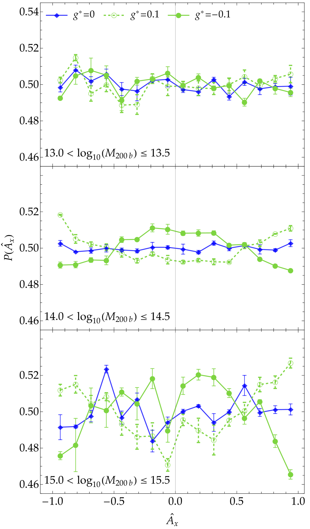
Figure 5: PDFs of $\hat{A}_{x}$, $P(\hat{A}_{x})$, for the halo mass ranges of $\log_{10}[M_{\rm 200b}/(h^{-1}M_{\odot})]\in(13,~13.5],~(14,~14.5]$ and $(15,~15.5]$. Each line shows the results for $g_{*}=0$ and $\pm 0.1$.

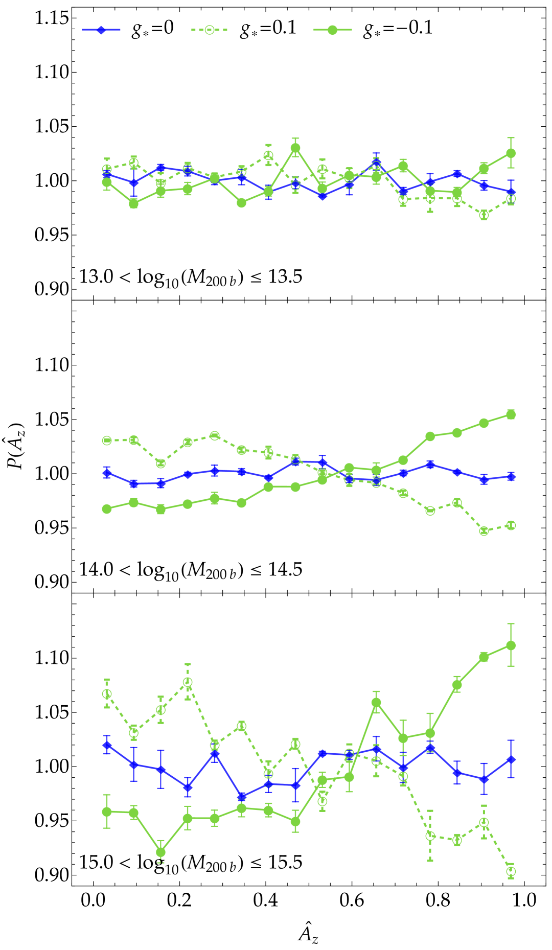
Figure 6: Same as Fig. 5 but for the PDFs of $\hat{A}_{z}$, $P(\hat{A}_{z})$.

Figs. 5 and 6 show the mass dependence of the modification of PDFs of $\hat{A}_{x}$ and $\hat{A}_{z}$ due to the SA, respectively. From top to bottom, we show the results for the halo mass ranges $\log_{10}[M_{\rm 200b}/(h^{-1}M_{\odot})]\in(13,~13.5]$, $(14,~14.5]$, and $(15,~15.5]$. The correspondence between line type and $g_{*}$ values is the same as in Fig. 4. We omit $P(\hat{A}_{y})$ here, as it is nearly identical to $P(\hat{A}_{x})$ due to the symmetry. For $g_{*}=\pm 0.1$, $P(\hat{A}_{x})$ and $P(\hat{A}_{z})$ show negligible deviations from the isotropic case in the lowest mass range, while the deviations become more pronounced in the $(14,~14.5]$ bin and even stronger in $(15,~15.5]$, maintaining the same $g_{*}$-dependence as in Fig. 4. These results suggest stronger SA-induced alignment for more massive halos. This trend is physically reasonable, as more massive halos have larger volumes roughly proportional to their mass and can more effectively “feel” global effects such as SA.

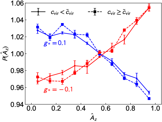
Figure 7: PDF of $\hat{A}_{z}$ for the high- and low-$c_{\rm vir}$ halos of $14<\log_{10}[M_{\rm 200b}/(h^{-1}M_{\odot})]\leq 14.5$ from the L2 run with $g_{*}=\pm 0.1$.

We also examine whether additional factors influence the alignment of halos induced by the SA. In particular, we investigate the correlation between the halo formation epoch and its alignment. It is well established that the halo concentration parameter serves as a reliable proxy for the formation epoch [35]. We define the halo concentration parameter as

$$c_{\rm vir}=R_{\rm vir}/r_{\rm s}~,$$ (6)

where $R_{\rm vir}$ and $r_{\rm s}$ are, respectively, the virial radius of the halo and the scale radius of the NFW density profile, $\rho_{\rm NFW}(r)=\rho_{\rm s}/[(r/r_{\rm s})(1+r/r_{\rm s})^{2}]$ [36]. We adopt the values of $R_{\rm vir}$ and $r_{\rm s}$ obtained from the Rockstar halo finder. We divide the halos of $14<\log_{10}[M_{\rm 200b}/(h^{-1}M_{\odot})]\leq 14.5$ from the L2 run with $g_{*}=\pm 0.1$ into two groups based on $c_{\rm vir}$: those with concentrations larger and smaller than the median value ${\tilde{c}}_{\rm vir}$. Fig. 7 shows the distribution function of $\hat{A}_{z}$ for the halos with high and low $c_{\rm vir}$. For both values of $g_{*}$, halos with higher and lower concentrations exhibit similar alignment distributions, indicating that the formation epoch does not significantly affect halo alignment associated with the SA. We found the same trend when halos were divided based on the triaxiality parameter $T$ as well as for halos with masses in the range in $15<\log_{10}[M_{\rm 200b}/(h^{-1}M_{\odot})]\leq 15.5$ in the $g_{*}=\pm 0.1$ case. These results suggest that the initial conditions influenced by SA are the primary factor responsible for the halo alignment in the statistically anisotropic universe.

IV conclusion

In this work, we investigated the impact of the SA in the matter density field on the shapes and orientations of cluster-sized halos at $z=0$ using cosmological $N$-body simulations that incorporate a quadrupolar-type SA characterized by the magnitude parameter $g_{*}$. For halo shapes, we examined the three-dimensional axis ratio $s$ (smallest-to-largest) and the triaxiality parameter $T$. Halo orientations were represented by the direction of the largest axis as ellipsoid, denoted by the vector $\mathbf{\hat{A}}$. We found that, while both of the shape parameters, $s$ and $T$, show little sensitivity to SA (Figs. 2 and 3), the halo orientations are significantly affected (Fig. 4). We also found that halo orientations tend to align perpendicular to the SA-preferred direction $\hat{\mathbf{d}}$ for positive values of $g_{*}$, and parallel for negative values (Fig. 4).

We used halos with masses of $\log_{10}[M_{\rm 200b}/(h^{-1}M_{\odot})]\in(13,~13.5]$, $(14,~14.5]$, and $(15,~15.5]$, and investigated the mass dependence of the alignment due to the SA. We clearly showed that this SA alignment effect becomes more pronounced for more massive halos, suggesting that more massive halos are more sensitive to the global anisotropic nature of the matter distribution (Figs. 5 and 6). Importantly, this alignment is expected to originate from the initial conditions that have inherent information about the SA, rather than later-stage nonlinear processes, as we found no significant dependence on halo properties such as concentration or ellipticity (Fig. 7).

In this paper, we employed a very simple scale-independent quadrupole type of SA, but other types of SA are actually possile. In fact, in the context of the inflation models with gauge fields including the anisotorpic inflation, the possibility of generating various types of SA has been actively discussed, e.g., statistically anisotropic non-Gaussianity (see, e.g., Ref. [37]), the SA in the primordial gravitational waves (see, e.g., Ref. [38]), and so on. In conjunction with those observations, it would be interesting to apply our analysis to more specific model-based types of SA to verify the early universe.

As the PDFs presented in this paper are one-point functions, they are insensitive to spatial correlations in halo orientations. However, the SA-induced changes in halo orientations may have implications for other cosmological observables, such as intrinsic alignments (IA) [32, 33, 34] (see also Refs. [39, 40] for recent studies on the IA of galaxy clusters). Since these effects could be potential sources of systematic errors in cosmological analyses or serve as tools to constrain the SA parameter, investigating how SA influences a broader range of statistical measures is an important direction for future work.

Our findings highlight the potential of using halo alignment as a complementary probe of the SA in the Universe. In particular, measurements of projected halo ellipticity, which is observable in galaxy cluster-galaxy lensing observations, would exhibit systematic directional features due to the SA-induced alignment and could be used to constrain $g_{*}$. Further works, including projection effects, redshift evolution, and connections to observable quantities, will be necessary to assess the feasibility of such constraints in future surveys.