Flattening Hierarchies with Policy Bootstrapping

Abstract

Offline goal-conditioned reinforcement learning (GCRL) is a promising approach for pretraining generalist policies on large datasets of reward-free trajectories, akin to the self-supervised objectives used to train foundation models for computer vision and natural language processing. However, scaling GCRL to longer horizons remains challenging due to the combination of sparse rewards and discounting, which obscures the comparative advantages of primitive actions with respect to distant goals. Hierarchical RL methods achieve strong empirical results on long-horizon goal-reaching tasks, but their reliance on modular, timescale-specific policies and subgoal generation introduces significant additional complexity and hinders scaling to high-dimensional goal spaces. In this work, we introduce an algorithm to train a flat (non-hierarchical) goal-conditioned policy by bootstrapping on subgoal-conditioned policies with advantage-weighted importance sampling. Our approach eliminates the need for a generative model over the (sub)goal space, which we find is key for scaling to high-dimensional control in large state spaces. We further show that existing hierarchical and bootstrapping-based approaches correspond to specific design choices within our derivation. Across a comprehensive suite of state- and pixel-based locomotion and manipulation benchmarks, our method matches or surpasses state-of-the-art offline GCRL algorithms and scales to complex, long-horizon tasks where prior approaches fail.

1 Introduction

Goal-conditioned reinforcement learning (GCRL) specifies tasks by desired outcomes, alleviating the burden of defining reward functions over the state-space and enabling the training of general policies capable of achieving a wide range of goals. Offline GCRL extends this paradigm to leverage existing datasets of reward-free trajectories and has been likened to the simple self-supervised objectives that have been successful in training foundation models for other areas of machine learning (Yang et al., 2023; Park et al., 2024a). However, the conceptual simplicity of GCRL belies practical challenges in learning accurate value functions and, consequently, effective policies for goals requiring complex, long-horizon behaviors. These limitations call into question its applicability as a general and scalable objective for learning foundation policies (Black et al., 2024; Park et al., 2024d; Intelligence et al., 2025) that can be efficiently adapted to a diverse array of control tasks.

Hierarchical reinforcement learning (HRL) is commonly used to address these challenges and is particularly well-suited to the recursive subgoal structure of goal-reaching tasks, where reaching distant goals entails first passing through intermediate subgoal states. Goal-conditioned HRL exploits this structure by learning a hierarchy composed of multiple levels: one or more high-level policies, tasked with generating intermediate subgoals between the current state and the goal; and a low-level actor, which operates over the primitive action space to achieve the assigned subgoals. These approaches have achieved state-of-the-art results in both online (Nachum et al., 2018; Levy et al., 2019) and offline GCRL (Park et al., 2024c), and are especially effective in long-horizon tasks. However, despite the strong empirical performance of HRL, it suffers from major limitations as a scalable pretraining strategy. In particular, the modularity of hierarchical policy architectures, fixed to specific levels of temporal abstraction, precludes unified task representations and necessitates learning a generative model over the subgoal space to interface between policy levels.

Learning to predict intermediate goals in a space that may be as high-dimensional as the raw observations poses a difficult generative modeling problem. To ensure that subgoals are physically realistic and reachable in the allotted time, previous work often implements additional processing and verification of proposed subgoals (Zhang et al., 2020; Hatch et al., 2024; Czechowski et al., 2024; Zawalski et al., 2024). An alternative is to instead predict in a compact learned latent subgoal space, but simultaneously optimizing subgoal representations and policies results in a nonstationary input distribution to the low-level actor, which can slow and destabilize training (Vezhnevets et al., 2017; Levy et al., 2019). The choice of objective for learning such representations, ranging from autoregressive prediction (Seo et al., 2022; Zeng et al., 2023) to metric learning (Tian et al., 2020; Nair et al., 2023; Ma et al., 2023), remains an open question and adds significant complexity to the design and tuning of hierarchical methods.

Following the tantalizing promise that flat, one-step policies can be optimal in fully observable, Markovian settings (Puterman, 2005), this work aims to isolate the core advantages of hierarchies for offline GCRL and distill them into a simpler training recipe for a single, unified policy. We begin our empirical analysis by revisiting a state-of-the-art hierarchical method for offline GCRL that significantly outperforms previous approaches on a range of long-horizon goal-reaching tasks. Beyond the original explanation based on improved value function signal-to-noise ratio, we find that separately training a low-level policy on nearby subgoals improves sampling efficiency. We reframe this hierarchical approach as a form of implicit test-time bootstrapping on subgoal-conditioned policies, revealing a conceptual connection to earlier methods that learn subgoal generators and bootstrap directly from subgoal-conditioned policies to train a flat, unified goal-conditioned policy.

Building on these insights, we present an inference-based theoretical framework that unifies these ideas and yields Subgoal Advantage-Weighted Policy Bootstrapping (SAW), a novel policy extraction objective for offline GCRL. SAW uses advantage-weighted importance sampling to bootstrap on subgoals sampled directly from data, capturing the long-horizon strengths of hierarchies in a single, flat policy without requiring a generative subgoal model. In evaluations across 20 state- and pixel-based offline GCRL datasets, our method matches or surpasses all baselines in diverse locomotion and manipulation tasks and scales especially well to complex, long-horizon tasks, being the only existing approach to achieve nontrivial success in the humanoidmaze-giant environment.

2 Related Work

Our work builds on a rich body of literature encompassing goal-conditioned RL (Kaelbling, 1993), offline RL (Lange et al., 2012; Levine et al., 2020), and hierarchical RL (Dayan & Hinton, 1992; Sutton et al., 1999; Stone, 2008; Bacon et al., 2016; Vezhnevets et al., 2017). The generality of the GCRL formulation enables powerful self-supervised training strategies such as hindsight relabeling (Andrychowicz et al., 2018; Ghosh et al., 2020) and state occupancy matching (Ma et al., 2022). These are often combined with approaches that exploit the recursive subgoal structure of GCRL: either implicitly via quasimetric learning (Wang et al., 2023), probabilistic interpretations (Hoang et al., 2021; Zhang et al., 2021b), and contrastive learning (Eysenbach et al., 2022; Zheng et al., 2024); or explicitly through hierarchical decomposition into subtasks (Nachum et al., 2018; Levy et al., 2019; Gupta et al., 2020; Park et al., 2024c). Despite these advances, learning remains difficult for distant goals due to sparse rewards and discounting over time. Many methods use the key insight that actions which are effective for reaching an intermediate subgoal between the current state and the goal are also effective for reaching the final goal. Such subgoals are typically selected via planning (Huang et al., 2019; Zhang et al., 2021a; Hafner et al., 2022), searching within the replay buffer (Eysenbach et al., 2019), or, most commonly, sampling from generative models. Hierarchical methods in particular generate subgoals during inference and use them to query “subpolicies” trained on shorter horizon goals, which are generally easier to learn (Strehl et al., 2009; Azar et al., 2017). Our method also leverages the ease of training subpolicies to effectively learn long-horizon behaviors, but aims to learn a flat, unified policy while avoiding the complexity of training generative models to synthesize new subgoals.

Policy bootstrapping. Our work is most closely related to Reinforcement learning with Imagined Subgoals (Chane-Sane et al., 2021, RIS), which, to our knowledge, is the only prior work that performs bootstrapping on policies, albeit in the online setting. Similar to goal-conditioned hierarchies, RIS learns a generative model to synthesize “imagined” subgoals that lie between the current state and the goal. Unlike HRL approaches, however, it regresses the full-goal-conditioned policy towards the subgoal-conditioned target, treating the latter as a prior to guide learning and exploration [Figure 1]. While RIS yields a flat policy for inference, it still requires the full complexity of a hierarchical policy, including a generative model over the goal space. In contrast, our work extends the core benefits of subgoal-based bootstrapping to offline GCRL with an advantage-based importance weight on subgoals sampled from dataset trajectories, eliminating the need for a subgoal generator altogether.

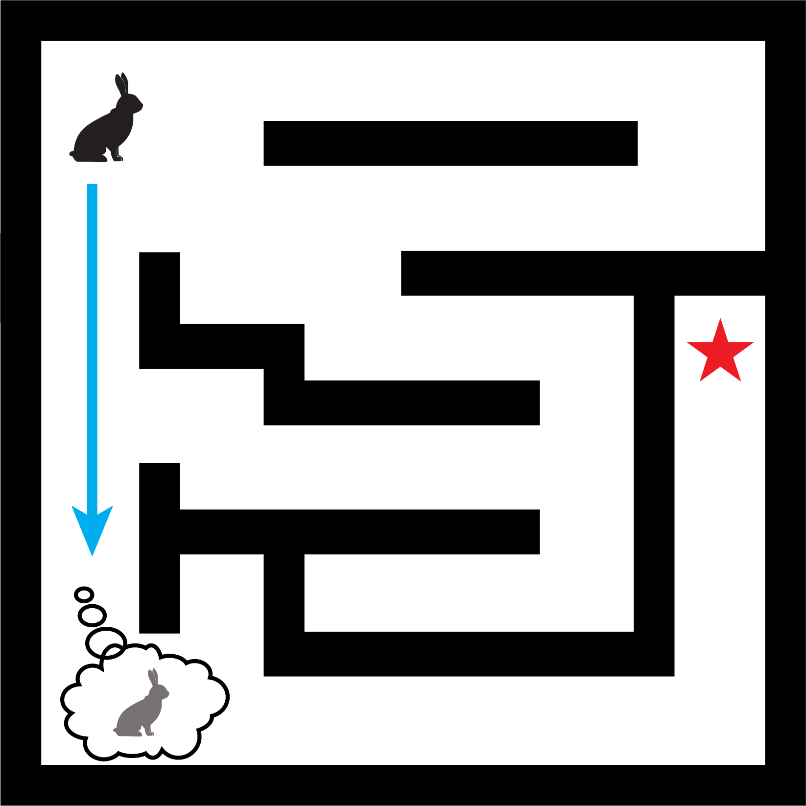
(a) HIQL

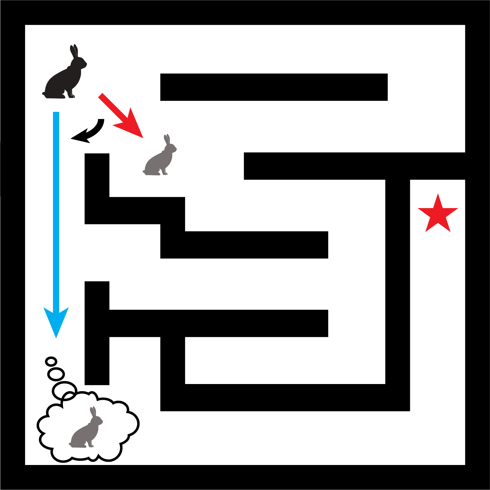
(b) RIS

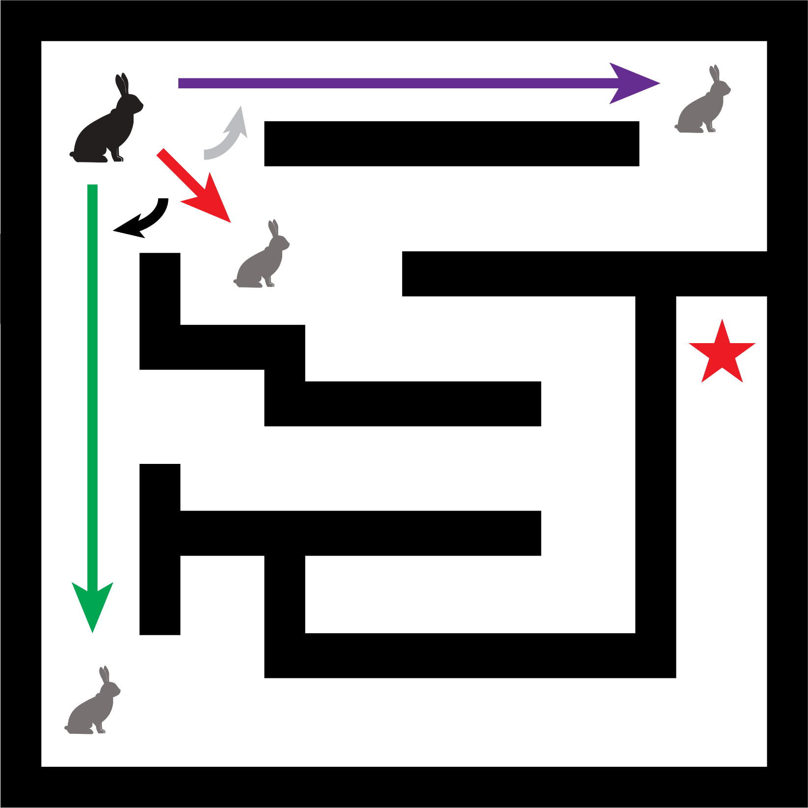
(c) SAW

Figure 1: Learning with subgoals. Both HIQL and RIS “imagine” subgoals (thought bubbles) en route to the goal (red star) with generative models. However, HIQL samples actions directly from the subgoal-conditioned policy, while RIS regresses (black arrow) a flat goal-conditioned policy towards the subgoal-conditioned action distribution during training. SAW also performs regression but only uses “real” subgoals from the dataset $\mathcal{D}$, weighting the regression more heavily towards distributions conditioned on good subgoals and less (gray arrow) towards bad ones.

3 Preliminaries

Problem setting: We consider the problem of offline goal-conditioned RL, described by a Markov decision process (MDP) $\mathcal{M}=(\mathcal{S},\mathcal{A},\mathcal{R},\mathcal{P})$ where $\mathcal{S}$ is the state space, $\mathcal{A}$ the action space, $\mathcal{R}:\mathcal{S}\times\mathcal{S}\rightarrow\mathbb{R}$ the goal-conditioned reward function (where we assume that the goal space $\mathcal{G}$ is equivalent to the state space $\mathcal{S}$), and $\mathcal{P}:\mathcal{S}\times\mathcal{A}\to\mathcal{S}$ the transition function. In the offline setting, we are given a dataset $\mathcal{D}$ of trajectories $\tau=(s_{0},a_{0},s_{1},a_{1},\ldots,s_{T})$ previously collected by some arbitrary policy (or multiple policies), and must learn a policy that can reach a specified goal state $g$ from an initial state $s_{0}\in\mathcal{S}$ without further interaction in the environment, maximizing the objective

$$J(\pi)=\mathbb{E}_{g\sim p(g),\tau\sim p^{\pi}(\tau)}\left[\sum_{t=0}^{\infty}\gamma^{t}r\left(s_{t},g\right)\right],$$ (1)

where $p(g)$ is the goal distribution and $p^{\pi}(\tau)$ is the distribution of trajectories generated by the policy $\pi$ and the transition function $\mathcal{P}$ during (online) evaluation.

Offline value learning: We use a goal-conditioned, action-free variant of implicit Q-learning (Kostrikov et al., 2021, IQL) referred to as goal-conditioned implicit value learning (Park et al., 2024c, GCIVL). The original IQL formulation modifies standard value iteration for offline RL by replacing the $\max$ operator with an expectile regression, in order to avoid value overestimation for out-of-distribution actions. GCIVL replaces the state-action value function with a value-only estimator

$$\min_{\psi}\mathcal{L}_{\mathrm{GCIVL}}(\psi)=\mathbb{E}_{s,a,g\sim p^{\mathcal{D}}}\left[\ell_{\tau}^{2}\left(r(s,g)+\gamma\bar{V}\left(s^{\prime},g\right)-V(s,g)\right)\right],$$ (2)

where $\ell_{\tau}^{2}(x)=|\tau-\mathbbm{1}(x<0)|x^{2}$ is the expectile loss parameterized by $\tau\in[0.5,1)$ and $\bar{V}(\cdot)$ denotes a target value function. Note that GCIVL is optimistically biased in stochastic environments, since it directly regresses towards high-value transitions without using Q-values to marginalize over action-independent stochasticity.

Offline policy extraction: To learn a target subpolicy, we use Advantage-Weighted Regression (Peng et al., 2019, AWR) to extracts a policy from a learned value function. AWR reweights state-action pairs according to their exponentiated advantage with an inverse temperature hyperparameter $\alpha$, via the objective

$$\max_{\pi}\mathcal{J}_{\mathrm{AWR}}(\pi)=\mathbb{E}_{s,a,g\sim\mathcal{D}}\left[e^{\alpha(Q(s,a,g)-V(s,g))}\log\pi(a\mid s,g)\right],$$ (3)

thus remaining within the support of the data without requiring an additional behavior cloning penalty.

4 Understanding Hierarchies in Offline GCRL

In this section, we seek to identify the core reasons behind the empirical success of hierarchies in offline GCRL that can be used to guide the design of a simpler training objective for a flat policy. We first review previous explanations for the benefits of HRL and propose an initial algorithm that seeks to capture these benefits in a flat policy, but find that it still fails to close the performance gap to Hierarchical Implicit Q-Learning (Park et al., 2024c, HIQL), a state-of-the art method. We then identify an additional practical benefit of hierarchical training schemes and show how HIQL exploits this from a policy bootstrapping perspective.

4.1 Hierarchies in online and offline GCRL

Previous investigations into the benefits of hierarchical RL in the online setting attribute their success to improved exploration (Stone, 2008) and training value functions with multi-step rewards (Nachum et al., 2019). They demonstrate that augmenting non-hierarchical agents in this manner can largely close the performance gap to hierarchical policies. However, the superior performance of hierarchical methods in the offline GCRL setting, where there is no exploration, calls this conventional wisdom into question.

HIQL is a state-of-the-art hierarchical offline GCRL method that extracts a high-level policy over subgoals and a low-level policy over primitive actions from a single goal-conditioned value function trained using standard one-step temporal difference learning. HIQL achieves significant performance gains across a number of complex, long-horizon navigation tasks purely through improvement on the policy extraction side, without needing multi-step rewards to train the value function as done in Nachum et al. (2019). While this does not preclude the potential benefits of multi-step rewards for offline GCRL, it does demonstrate that the advantages of hierarchies are not limited to temporally extended value learning, in line with previous claims that the primary bottleneck in offline RL is policy extraction and not value learning (Park et al., 2024b).

4.2 Value signal-to-noise ratio in offline GCRL

Instead, HIQL addresses a separate “signal-to-noise ratio” (SNR) issue in value functions conditioned on distant goals, where a combination of sparse rewards and discounting makes it nearly impossible to accurately determine the advantage of one primitive action over another with respect to distant goals. By separating policy extraction into two levels, the low-level actor can instead evaluate the relative advantage of actions with respect to nearby subgoals and the high-level policy can utilize multi-step advantage estimates to get a clearer learning signal with respect to distant goals.

To test whether improved SNR in advantage estimates with respect to distant goals is indeed the key to HIQL’s superior performance, we propose to utilize subgoals to directly improve advantage estimates in a simple baseline method we term goal-conditioned waypoint advantage estimation (GCWAE). Briefly, we use the advantage of actions with respect to subgoals generated by a high-level policy as an estimator of the undiscounted advantage with respect to the true goal

$$\tilde{A}(s_{t},a_{t},g)\approx A\left(s_{t},a_{t},w\right),$$ (4)

where $w\sim\pi^{h}_{\text{sg}}(w\mid s_{t},g)$ is a subgoal sampled from a high-level policy $\pi^{h}$, and the sg subscript indicates a stop-gradient operator. Apart from using this advantage to directly train a flat policy with AWR, we use the same architectures, sampling distributions, and training objective for $\pi^{h}$ as HIQL. Despite large gains over one-step policy learning objectives in several navigation tasks, GCWAE still underperforms its hierarchical counterpart, achieving a 55% success rate on antmaze-large-navigate compared to 90% for HIQL without subgoal representations and 16% for GCIVL with AWR.

4.3 It’s easier to find good (dataset) actions for closer goals

While diagnosing this discrepancy, we observed that training statistics for the two methods were largely identical except for a striking difference in the mean action advantage $A(s_{t},a_{t},w)$. The advantage was significantly lower for GCWAE, which samples “imagined” subgoals $w\sim\pi^{h}(\cdot\mid s,g)$ from a high-level policy, than HIQL, which samples directly from the $k$-step future state distribution $w\sim p^{\mathcal{D}}(s_{t+k}\mid s_{t})$ of the dataset. This leads us to an obvious but important insight: in most cases, dataset actions are simply better with respect to subgoals sampled from nearby future states in the trajectory than to distant goals or “imagined” subgoals generated by a high-level policy. The dataset is far more likely to contain high-advantage actions for goals sampled at the ends of short subsequences, whereas optimal state-action pairs for more distant goals along the trajectory are much rarer due to the combinatorial explosion of possible goal states as the goal-sampling horizon increases.

The practical benefits of being able to easily sample high-advantage state-action-goal tuples are hinted at in Park et al. (2024a), who pose the question “Why can’t we use random goals when training policies?” after finding that offline GCRL algorithms empirically perform better when only sampling (policy) goals from future states in the same trajectory as the initial state. While their comparison focuses on in-trajectory versus random goals instead of nearer versus farther in-trajectory goals, we hypothesize both observations are driven by similar explanations.

4.4 Hierarchies perform test-time policy bootstrapping

Our observations suggest that training policies on nearby goals benefits both from better value SNR in advantage estimates and the ease of sampling good state-action-goal combinations. For brevity, we will refer to such policies trained only on goals of a restricted horizon length as “subpolicies," denoted by $\pi^{\mathrm{sub}}$ and analogous to the low-level policies $\pi^{\ell}$ in hierarchies. Now we ask: how do hierarchical methods take advantage of the relative ease of training subpolicies to reach distant goals, and can we use similar strategies to train flat policies?

HIQL separately trains a low-level subpolicy on goals sampled from states at most $k$ steps into the future, reaping all the benefits of policy training with nearby goals. Similar to other goal-conditioned hierarchical methods (Nachum et al., 2018; Levy et al., 2019), it then uses the high-level policy to predict optimal subgoals between the current state and the goal at test time, and “bootstraps” by using the subgoal-conditioned action distribution as an estimate for the full goal-conditioned policy.

5 Subgoal Advantage-Weighted Policy Bootstrapping

We now seek to unify the above insights into an objective to learn a single, flat goal-reaching policy without the additional complexity of HRL. Following the bootstrapping perspective, a direct analogue to hierarchies would use the subpolicy to construct training targets, regressing the full goal-conditioned policy towards a target subpolicy conditioned on the output of a subgoal generator $P\left(a\mid s,\pi^{h}(w\mid s,g)\right)$. This approach, taken by RIS [Figure 1], still inherits the full complexity of hierarchical policies and then some: it requires learning a subgoal generator, a subpolicy, and an additional flat policy.

5.1 Hierarchical RL as inference

To eliminate this additional machinery, we adopt the view of GCRL as probabilistic inference (Levine, 2018). In this framing, the bilevel objectives for HIQL’s hierarchical policy and the KL bootstrapping term for RIS’s flat policy can be derived from the same inference problem with different choices of variational posterior. Our main insight is that the expectation over generated subgoals can be expressed as an expectation over the dataset distribution with an advantage-based importance weight, yielding our SAW objective. We present an abridged version below and leave the full derivation to Appendix C.

Similar to previous work (Abdolmaleki et al., 2018), we cast the infinite-horizon, discounted GCRL formulation as an inference problem by constructing a probabilistic model via the likelihood function $p\left(U=1\mid\tau,\{w\},g\right)\propto\exp\left(\beta\sum_{t=0}^{\infty}\gamma^{t}A\left(s_{t},w_{t},g\right)\right)$, where the binary variable $U$ can be interpreted as the event of reaching the goal $g$ as quickly as possible from state $s_{t}$ by passing through subgoal state $w$. The subgoal advantage is defined as $A(s_{t},w,g)=-V(s_{t},g)+\gamma^{k}V(w,g)+\sum_{t^{\prime}=t}^{k-1}r(s_{t^{\prime}},g)$, where $w\sim p^{\mathcal{D}}(s_{t+k}\mid s_{t})$. In practice, we follow HIQL and simplify the advantage estimate to $V(w,g)-V(s_{t},g)$, i.e., the progress towards the goal achieved by reaching $w$.

Without loss of generality (since we can represent any flat Markovian policy simply by setting $\pi^{h}(\cdot\mid s,g)$ to a point distribution on $g$), we use an inductive bias on the subgoal structure of GCRL to consider prior distributions $\pi$ of a factored hierarchical form

$$p_{\pi}(\tau\mid g)=p(s_{0})\prod^{\infty}_{t=0}p(s_{t+1}\mid s_{t},a_{t})\pi^{\ell}(a_{t}\mid s_{t},w_{t})\pi^{h}(w_{t}\mid s_{t},g).$$

The distinctions between hierarchical approaches like HIQL and non-hierarchical approaches such as RIS and SAW begin with our choice of variational posterior. For the former, we would consider similarly factored distributions, whereas for the latter, we use a flat policy $\pi_{\theta}(\tau\mid g)$ that factors as

$$\pi_{\theta}(\tau\mid g)=p(s_{0})\prod^{\infty}_{t=0}p(s_{t+1}\mid s_{t},a_{t})\pi_{\theta}(a_{t}\mid s_{t},g),$$

assuming that the dataset policies are Markovian. We also introduce a variational posterior $q(\{w\}\mid g)$ which factors over a sequence of waypoints $\{w\}=\{w_{0},w_{1},\ldots\}$ as

$$q(\{w\}\mid g)=p(s_{0})\prod^{\infty}_{t=0}p(s_{t+1}\mid s_{t},a_{t})\pi^{\mathrm{sub}}(a_{t}\mid s_{t},w_{t})q(w_{t}\mid s_{t},g).$$

where we treat the target subpolicy $\pi^{\mathrm{sub}}$ as fixed. Using these definitions, we define the evidence lower bound (ELBO) on the optimality likelihood $p_{\pi}(U=1)$ for policy $\pi$ and goal distribution $p(g)$

$$\log p_{\pi}(U=1) =\log\int p(g)p_{\pi}(\tau,\{w\}\mid g)p(U=1\mid\tau,\{w\},g)d\{w\}\,d\tau\,dg$$

$$\geq\mathbb{E}_{\pi_{\theta}(\tau\mid g),q(\{w\}\mid g),p(g)}\log\left[\frac{p(U=1,\tau,\{w\}\mid g)}{\pi_{\theta}(\tau\mid g)q(\{w\}\mid g)}\right]=\mathcal{J}(\pi_{\theta},q).$$

Expanding distributions according to their factorizations, dropping terms that are independent of the variationals, and rewriting the discounted sum over time as an expectation over the (unnormalized) discounted stationary state distribution $\mu_{\pi}(s)=\sum_{t=0}^{\infty}\gamma^{t}p(s_{t}=s\mid\pi)$ results in the final objective

$$\mathcal{J}(\theta,q)=\mathbb{E}_{\mu(s),p(g)}\big{[}\mathbb{E}_{q(w\mid s,g)}\left[A(s,w,g)\right] -\mathbb{E}_{\pi_{\theta}(a\mid s,g)}\left[D_{\mathrm{KL}}(q(w\mid s,g)\|\pi^{h}(w\mid s,g))\right]$$

$$-\mathbb{E}_{q(w\mid s,g)}\left[D_{\mathrm{KL}}(\pi_{\theta}(a\mid s,g)\|\pi^{\ell}(a\mid s,w))\right]\big{]},$$ (5)

where we optimize an approximation of $\mathcal{J}$ by sampling from the dataset distribution $\mu_{\mathcal{D}}(s)$ (Schulman et al., 2017; Abdolmaleki et al., 2018; Peng et al., 2019).

Algorithm 1 Subgoal Advantage-Weighted Policy Bootstrapping (SAW)

1: Input: offline dataset $\mathcal{D}$, goal distribution $p(g)$.

2: Initialize value function $V_{\phi}$, target subpolicy $\pi_{\psi}$, and policy $\pi_{\theta}$.

3: while not converged do

4:  Train value function: $\phi\leftarrow\phi-\lambda\nabla_{\phi}\mathcal{L}_{\mathrm{GCIVL}}(\phi)$ with $(s_{t},s_{t+1})\sim p^{\mathcal{D}},g\sim p(g)$ [Equation 2]

5: end while

6: while not converged do

7:  Train target subpolicy: $\psi\leftarrow\psi-\lambda\nabla_{\psi}\mathcal{J}_{\mathrm{AWR}}(\psi)$ with $(s_{t},a,w)\sim p^{\mathcal{D}}$ [Equation 3]

8: end while

9: while not converged do

10:  Train policy: $\theta\leftarrow\theta-\lambda\nabla_{\theta}\mathcal{J}_{\mathrm{SAW}}(\theta)$ with $(s_{t},a,w)\sim p^{\mathcal{D}},g\sim p(g)$ [Equation 7]

11: end while

5.2 Eliminating the subgoal generator

Both RIS and HIQL directly parameterize $q(w\mid s,g)$ with a subgoal generator and optimize according the first line of Equation 5.1, which can be solved analytically and results in an objective similar to AWR [Equation 3] when projected into the space of parameterized policies

$$\mathcal{J}(q) =\mathbb{E}_{\mu(s),p(g)}\left[\mathbb{E}_{q(w\mid s,g)}[A(s,w,g)]-\mathbb{E}_{\pi_{\theta}(a\mid s,g)}\left[D_{\mathrm{KL}}(q(w\mid s,g)\|\pi^{h}(w\mid s,g))\right]\right]$$

$$\propto\mathbb{E}_{\mu(s),p(g)}\left[\exp(A(s,w,g))\log q(w\mid s,g)\right].$$

Then, RIS trains a flat policy $\pi_{\theta}$ using the third term in Equation 5.1, which is an expectation over the subgoals generated by $q$. Our key insight is that, rather than learning a generative model to approximate $p(w\mid s,g,U=1)$, we can instead use a simple application of Bayes’ rule:

$$p(w\mid s,g,U=1) \propto p^{\mathcal{D}}(w\mid s)p(U=1\mid s,w,g)$$

$$\propto p^{\mathcal{D}}(w\mid s)\exp(A(s,w,g)),$$

which replaces the expectation over $q$ to yield our subgoal advantage-weighted bootstrapping term

$$\mathbb{E}_{\mu(s),p^{\mathcal{D}}(w\mid s),p(g)}[\exp(A(s,w,g))D_{\mathrm{KL}}(\pi_{\theta}(a\mid s,g)\|\pi^{\ell}(a\mid s,w))].$$ (6)

We separately learn an approximation to $\pi^{\ell}(a\mid s,w)$, which we do in practice by training a target subpolicy with AWR in a similar fashion to HIQL (whereas RIS uses a exponential moving average of its online goal-conditioned policy as a target). While we omit this for clarity, a subpolicy AWR term can be incorporated into our objective by introducing another optimality variable $p\left(O_{t}=1\mid\tau,\{w\}\right)$ and a posterior for $\pi^{\ell}$, similar to our derivation for HIQL in Appendix C.

While approximating $p(w\mid s,U=1)$ with $q$ directly and using our importance weight on the dataset distribution are mathematically equivalent, the latter does introduce sampling-based limitations, which we discuss in Appendix A. However, we show empirically that the benefits from lifting the burden of learning a distribution over a high-dimensional subgoal space far outweigh these drawbacks, especially in large state spaces with high intrinsic dimensionality.

5.3 The SAW objective

The importance weight in Equation 6 allows the policy to bootstrap from subgoals sampled directly from dataset trajectories by ensuring that only subpolicies conditioned on high-advantage subgoals influence the direction of the goal-conditioned policy. We combine our bootstrapping term with an additional learning signal from a (one-step) policy extraction objective utilizing the value function, which improves performance in stitching-heavy environments [Appendix H]. Here, we use one-step AWR [Equation 3], yielding the full SAW objective:

$$\mathcal{J}(\theta)=\mathbb{E}_{p^{\mathcal{D}}(s,a,w),p(g)}{\left[e^{\alpha A(s,a,g)}\log\pi_{\theta}(a\mid s,g)-e^{\beta A(s,w,g)}D_{\mathrm{KL}}\left(\pi_{\theta}(\cdot\mid s,g)\|\pi^{\mathrm{sub}}_{\psi}(\cdot\mid s,w)\right)\right]}$$ (7)

where $\alpha$ and $\beta$ are inverse temperature hyperparameters. This objective provides a convenient dynamic balance between its two terms: as the goal horizon increases, the differences in action values and therefore the contribution of one-step term decreases. This, in turn, downweights the noisier value-based learning signal and shifts emphasis toward the policy bootstrapping term. Finally, we use GCIVL to learn $V$, resulting in the full training scheme outlined in Algorithm 1.

6 Experiments

To assess SAW’s ability to reason over long horizons and handle high-dimensional observations, we conduct experiments across 20 datasets corresponding to 7 locomotion and manipulation environments [Figure 2] with both state- and pixel-based observation spaces. We report performance averaged over 5 state-goal pairs for each dataset, yielding $\mathbf{100}$ total evaluation tasks. Implementation details and hyperparameter settings are discussed in Appendices F and G, respectively.

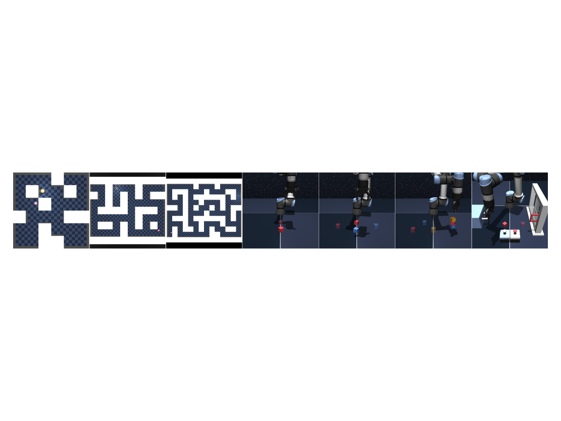
Figure 2: OGBench tasks. We train SAW on 20 datasets collected from 7 different environments (pictured above) and perform evaluations across 5 state-goal pairs for each dataset.

6.1 Experimental setup

We select several environments and their corresponding datasets from the recently released OGBench suite (Park et al., 2024a), a comprehensive benchmark specifically designed for offline GCRL. OGBench provides multiple state-goal pairs for evaluation and datasets tailored to evaluate desirable properties of offline GCRL algorithms, such as the ability to reason over long horizons and stitch across multiple trajectories or combinatorial goal sequences. We use the baselines from the original OGBench paper, which include both one-step and hierarchical state-of-the-art offline GCRL methods. We briefly describe each category of tasks below and baseline algorithms in Appendix D, and encourage readers to refer to the Park et al. (2024a) for further details.

Locomotion: Locomotion tasks require the agent to control a simulated robot to navigate through a maze and reach a designated goal. The agent embodiment varies from a simple 2D point mass with two-dimensional action and observation spaces to a humanoid robot with 21 degrees of freedom and a 69-dimensional state space. In the visual variants, the agent receives a third-person, egocentric $64\times 64\times 3$ pixel-based observations, with its location within the maze indicated by the floor color. Maze layouts range from medium to giant, where tasks in the humanoidmaze version of the latter require up to 3000 environment steps to complete.

Manipulation: Manipulation tasks use a 6-DoF UR5e robot arm to manipulate object(s), including up to four cubes and a more diverse scene environment that includes buttons, windows, and drawers. The multi-cube and scene environments are designed to test an agent’s ability to perform sequential, long-horizon goal stitching and compose together multiple atomic behaviors. The visual variants also provide $64\times 64\times 3$ pixel-based observations where certain parts of the environment and robot arm are made semitransparent to ease state estimation.

Table 1: Evaluating SAW on state- and pixel-based offline goal-conditioned RL tasks. We compare our method’s average (binary) success rate ($\%$) against the numbers reported in Park et al. (2024a) across the five test-time goals for each environment, averaged over $8$ seeds ($4$ seeds for pixel-based visual tasks) with standard deviations after the $\pm$ sign. Numbers within $5\%$ of the best value in the row are in bold. Results with an asterisk (^∗) use different value learning hyperparameters and are discussed further in Section 6.3.

Environment	Dataset	GCBC	GCIVL	GCIQL	QRL	CRL	HIQL	SAW
pointmaze	pointmaze-medium-navigate-v0	$9$ $\pm 6$	$63$ $\pm 6$	$53$ $\pm 8$	$82$ $\pm 5$	$29$ $\pm 7$	$79$ $\pm 5$	$\mathbf{97}$ $\pm 2$
	pointmaze-large-navigate-v0	$29$ $\pm 6$	$45$ $\pm 5$	$34$ $\pm 3$	$\mathbf{86}$ $\pm 9$	$39$ $\pm 7$	$58$ $\pm 5$	$\mathbf{85}$ $\pm 10$
	pointmaze-giant-navigate-v0	$1$ $\pm 2$	$0$ $\pm 0$	$0$ $\pm 0$	$\mathbf{68}$ $\pm 7$	$27$ $\pm 10$	$46$ $\pm 9$	$\mathbf{68}$ $\pm 8$
antmaze	antmaze-medium-navigate-v0	$29$ $\pm 4$	$72$ $\pm 8$	$71$ $\pm 4$	$88$ $\pm 3$	$\mathbf{95}$ $\pm 1$	$\mathbf{96}$ $\pm 1$	$\mathbf{97}$ $\pm 1$
	antmaze-large-navigate-v0	$24$ $\pm 2$	$16$ $\pm 5$	$34$ $\pm 4$	$75$ $\pm 6$	$83$ $\pm 4$	$\mathbf{91}$ $\pm 2$	$\mathbf{90}$ $\pm 3$
	antmaze-giant-navigate-v0	$0$ $\pm 0$	$0$ $\pm 0$	$0$ $\pm 0$	$14$ $\pm 3$	$16$ $\pm 3$	${65}$ $\pm 5$	$\mathbf{73}$ $\pm 4$
humanoidmaze	humanoidmaze-medium-navigate-v0	$8$ $\pm 2$	$24$ $\pm 2$	$27$ $\pm 2$	$21$ $\pm 8$	$60$ $\pm 4$	$\mathbf{89}$ $\pm 2$	$\mathbf{88}$ $\pm 3$
	humanoidmaze-large-navigate-v0	$1$ $\pm 0$	$2$ $\pm 1$	$2$ $\pm 1$	$5$ $\pm 1$	$24$ $\pm 4$	$\mathbf{49}$ $\pm 4$	${46}$ $\pm 4$
	humanoidmaze-giant-navigate-v0	$0$ $\pm 0$	$0$ $\pm 0$	$0$ $\pm 0$	$1$ $\pm 0$	$3$ $\pm 2$	${12}$ $\pm 4$	$\mathbf{35}$ $\pm 4$
cube	cube-single-play-v0	$6$ $\pm 2$	$53$ $\pm 4$	${68}$ $\pm 6$	$5$ $\pm 1$	$19$ $\pm 2$	$15$ $\pm 3$	$\mathbf{72}^{*}$ $\pm 5$
	cube-double-play-v0	$1$ $\pm 1$	$36$ $\pm 3$	$\mathbf{40}$ $\pm 5$	$1$ $\pm 0$	$10$ $\pm 2$	$6$ $\pm 2$	$\mathbf{40}$ $\pm 7$
	cube-triple-play-v0	$1$ $\pm 1$	$1$ $\pm 0$	$3$ $\pm 1$	$0$ $\pm 0$	$\mathbf{4}$ $\pm 1$	$3$ $\pm 1$	$\mathbf{4}$ $\pm 2$
scene	scene-play-v0	$5$ $\pm 1$	$42$ $\pm 4$	${51}$ $\pm 4$	$5$ $\pm 1$	$19$ $\pm 2$	$38$ $\pm 3$	$\mathbf{63}$ $\pm 6$
visual-antmaze	visual-antmaze-medium-navigate-v0	$11$ $\pm 2$	$22$ $\pm 2$	$11$ $\pm 1$	$0$ $\pm 0$	$\mathbf{94}$ $\pm 1$	$\mathbf{93}$ $\pm 4$	$\mathbf{95}$ $\pm 0$
	visual-antmaze-large-navigate-v0	$4$ $\pm 0$	$5$ $\pm 1$	$4$ $\pm 1$	$0$ $\pm 0$	$\mathbf{84}$ $\pm 1$	$53$ $\pm 9$	$\mathbf{82}$ $\pm 4$
	visual-antmaze-giant-navigate-v0	$0$ $\pm 0$	$1$ $\pm 1$	$0$ $\pm 0$	$0$ $\pm 0$	$\mathbf{47}$ $\pm 2$	$6$ $\pm 4$	$10$ $\pm 2$
visual-cube	visual-cube-single-play-v0	$5$ $\pm 1$	$60$ $\pm 5$	$30$ $\pm 5$	$41$ $\pm 15$	$31$ $\pm 15$	$\mathbf{89}$ $\pm 0$	$\mathbf{88}$ $\pm 3$
	visual-cube-double-play-v0	$1$ $\pm 1$	$10$ $\pm 2$	$1$ $\pm 1$	$5$ $\pm 0$	$2$ $\pm 1$	$\mathbf{39}$ $\pm 2$	$\mathbf{40}$ $\pm 3$
	visual-cube-triple-play-v0	$15$ $\pm 2$	$14$ $\pm 2$	$15$ $\pm 1$	$16$ $\pm 1$	$17$ $\pm 2$	$\mathbf{21}$ $\pm 0$	$\mathbf{20}$ $\pm 1$
visual-scene	visual-scene-play-v0	$12$ $\pm 2$	$25$ $\pm 3$	$12$ $\pm 2$	$10$ $\pm 1$	$11$ $\pm 2$	$\mathbf{49}$ $\pm 4$	$\mathbf{47}$ $\pm 6$

6.2 Locomotion results

State-based locomotion: As a method designed for long-horizon reasoning, SAW excels in all variants of the state-based locomotion tasks. It scales particularly well to long horizons, exhibiting the best performance of $\mathbf{73}\%$ across all tasks in antmaze-giant-navigate and is the first method to achieve non-trivial success in humanoidmaze-giant-navigate, reaching $\mathbf{35}\%$ success compared to the previous state-of-the-art of $12\%$ (Park et al., 2024a). We demonstrate that training subpolicies with subgoal representations scales poorly to the giant maze environments [Figure 3] but are critical to HIQL’s performance, emphasizing a fundamental tradeoff in hierarchical methods: subgoal representations are essential for making high-level policy prediction tractable, but those same representations can constrain policy expressiveness and limit overall performance. While other subgoal representation learning objectives may perform better than those derived from the value function, as in HIQL, this highlights the additional design complexity and tuning required for HRL methods. We also implement an offline variant of RIS [Appendix D] and find that it performs significantly worse than SAW with subgoal representations, which we suspect can be explained by our insights in Section 4.3.

Pixel-based locomotion: SAW maintains strong performance when given $64\times 64\times 3$ visual observations and scales much better to visual-antmaze-large than does its hierarchical counterpart. However, we do see a significant performance drop in the giant variant relative to the results in the state-based observation space. As a possible explanation for this discrepancy, we observed that value function training diverged for HIQL and SAW in visual-antmaze-giant as well as all visual-humanoidmaze sizes (omitted since no method achieved non-trivial performance). This occurred even without shared policy gradients, suggesting that additional work is needed to scale offline value learning objectives to very long-horizon tasks with high-dimensional visual observations.

6.3 Manipulation results

State-based manipulation: SAW consistently matches state-of-the-art performance in cube environments and significantly outperforms existing methods in the 5 scene tasks, which require extended compositional reasoning. Interestingly, we found that methods which use expectile regression-based offline value learning methods (GCIVL, GCIQL, HIQL, and SAW) are highly sensitive to value learning hyperparameters in the cube-single environment. Indeed, SAW performs more than twice as well on cube-single-play-v0 with settings of $\tau=0.9$ and $\beta=0.3$, reaching state-of-the-art performance ($\mathbf{72\%}$ $\pm 5$ vs. $32\%$ $\pm 4$ with $\tau=0.7$). While SAW is agnostic to the choice of value learning objective, we make special mention of these changes since they depart from the OGBench convention of fixing value learning hyperparameters for each method across all datasets.

Pixel-based manipulation: In contrast to the state-based environments, SAW and HIQL achieve near-equivalent performance in visual manipulation. This suggests that representation learning, and not long-horizon reasoning or goal stitching, is the primary bottleneck in the visual manipulation environments. While we do not claim any representation learning innovations for this paper, our results nonetheless demonstrate that SAW is able to utilize similar encoder-sharing tricks as HIQL to scale to high-dimensional observation spaces.

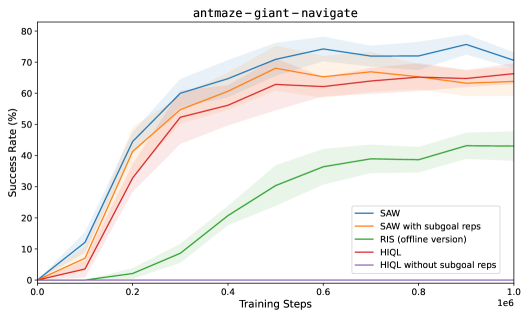
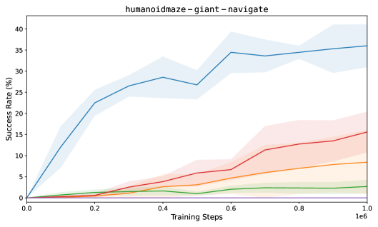
Figure 3: Subgoal representations scale poorly to high-dimensional control in large state spaces. Using HIQL’s subgoal representations (taken from an intermediate layer of the value function) for SAW’s target subpolicy harms performance compared to training directly on observations. However, HIQL fails to learn meaningful behaviors when predicting subgoals directly in the raw observation space. RIS, which bootstraps on generated subgoals at every step, performs the worst of the three.

7 Discussion

We presented Subgoal Advantage-Weighted Policy Bootstrapping (SAW), a simple yet effective policy extraction objective that leverages the subgoal structure of goal-conditioned tasks to scale to long-horizon tasks, without learning generative subgoal models. SAW consistently matches or surpasses current state-of-the-art methods across a wide variety of locomotion and manipulation tasks that require different timescales of control, whereas existing methods tend to specialize in particular task categories. Our method especially distinguishes itself in long-horizon reasoning, excelling in the most difficult locomotion tasks and scene-based manipulation. While the simplicity of our objective does introduce some practical limitations related to subgoal sampling, which we discuss in Appendix A, we find that avoiding explicit subgoal prediction is crucial for maintaining performance in large state spaces. By demonstrating a scalable approach to train unified policies for offline GCRL, we believe that SAW takes a step toward realizing the full potential of robotic foundation models in addressing the long-horizon, high-dimensional challenges of real-world control.

Appendix A Limitations

A theoretical limitation of our approach, which is common to all hierarchical methods as well as RIS, occurs in our assumption that the optimal policy can be represented in the factored form $\pi^{\ell}(a\mid s,w)\pi^{h}(w\mid s,g)$. While this is true in theory (since we could trivially set $\pi^{h}(w\mid s,g)$ to a point distribution at $g$), practical algorithms typically fix the distance of the subgoals to a shorter distance of $k$ steps (or the midpoint in RIS), where subgoals $s_{t+k}$ are sampled from the future state distribution $p^{\mathcal{D}}_{\mathrm{traj}}(s_{t+k}\mid s_{t})$. Intuitively, if the dataset contains only suboptimal trajectories towards waypoints occurring $k$ steps later which are reachable in fewer than $k$ steps with an optimal low-level policy $\pi^{\ell}$, then the space of sampled subgoals will not contain these further state-subgoal pairs and any approximation of $\pi^{h}(w\mid s,g,U=1)$ (whether an explicit subgoal generator or our importance-weighted approach), will suffer additional approximation gaps.

However, as discussed in Section 4.3, we find that subgoals sampled from the future state distribution empirically work well with respect to goals also sampled from the future state distribution, which is common in practice (Gupta et al., 2020; Ghosh et al., 2020; Yang et al., 2022; Eysenbach et al., 2022; Park et al., 2024c). However, we expect subgoal generator-based methods to have the edge when we sample from a goal distribution for which in-trajectory state-subgoal pairs tend to be highly suboptimal. While a generative subgoal model can synthesize “imagined” subgoals on which to bootstrap, our approach may require alternative subgoal-sampling strategies to reach the same level of performance.

Appendix B Planning Invariance

As an aside, we note that the discussions in this paper are closely related to the recently introduced concept of planning invariance (Myers et al., 2025), which describes a policy that takes similar actions when directed towards a goal as when directed towards an intermediate waypoint en route to that goal. In fact, we can say that subgoal-conditioned HRL methods achieve a form of planning invariance by construction, since they simply use the actions yielded by waypoint-conditioned policies to reach further goals. By minimizing the divergence between the full goal-conditioned policy and an associated subgoal-conditioned policy, both SAW and RIS can also be seen as implicitly enforcing planning invariance.

Appendix C Derivations of HIQL, RIS, and SAW Objectives

We cast the infinite-horizon, discounted GCRL formulation as an inference problem by constructing a probabilistic model via the likelihood function

$$p\left(U_{t}=1\mid\tau,\{w\},g\right)\propto\exp\left(\beta\sum_{t=0}^{\infty}\gamma^{t}A\left(s_{t},w_{t},g\right)\right),$$

where $\beta$ is an inverse temperature parameter and the binary variable $U$ can be intuitively understood as the event of reaching the goal $g$ as quickly as possible by passing through a subgoal $w$, or passing through a subgoal $w$ which is on the shortest path between $s_{t}$ and $g$.

We consider prior distributions $\pi$ of a factored hierarchical form

$$p_{\pi}(\tau\mid g)=p(s_{0})\prod^{\infty}_{t=0}p(s_{t+1}\mid s_{t},a_{t})\,\pi^{\ell}(a\mid s_{t},w_{t})\,\pi^{h}(w_{t}\mid s_{t},g).$$

C.1 HIQL derivation

Since HIQL learns two levels of a policy, we can use a variational posterior of the same form

$$\pi_{\theta,\psi}(\tau\mid g)=p(s_{0})\prod^{\infty}_{t=0}p(s_{t+1}\mid s_{t},a_{t})\,\pi^{\ell}_{\theta}(a_{t}\mid s_{t},w_{t})\,\pi^{h}_{\psi}(w_{t}\mid s_{t},g).$$

To incorporate training of the low-level policy, we also construct an additional probabilistic model for the optimality of primitive actions towards a waypoint $w$ (note that this can also be done to incorporate target policy training into the SAW objective, but we leave it out for brevity)

$$p\left(O_{t}=1\mid\tau,\{w\}\right)\propto\exp\left(\alpha\sum_{t=0}^{\infty}\gamma^{t}A\left(s_{t},a_{t},w_{t}\right)\right).$$

With these definitions, we define the evidence lower bound (ELBO) on the joint optimality likelihood $p_{\pi}(O=1,U=1)$ for policy $\pi$

$$\log p_{\pi}(O=1,U=1) =\log\int p(g)\,p(O=1,U=1,\tau,\{w\}\mid g)d\{w\}\,d\tau\,dg$$

$$=\log\int p(g)\pi_{\theta}(\tau\mid g)\pi_{\psi}(\{w\}\mid g)\frac{p(O=1,U=1,\tau,\{w\}\mid g)}{\pi_{\theta}(\tau\mid g)\,\pi_{\psi}(\{w\}\mid g)}d\{w\}\,d\tau\,dg$$

$$=\log\mathbb{E}_{\pi_{\theta}(\tau\mid g),\pi_{\psi}(\{w\}\mid g),p(g)}\left[\frac{p(O=1,U=1,\tau,\{w\}\mid g)}{\pi_{\theta}(\tau\mid g)\pi_{\psi}(\{w\}\mid g)}\right]$$

$$\geq\mathbb{E}_{\pi_{\theta}(\tau\mid g),\pi_{\psi}(\{w\}\mid g),p(g)}\log\left[\frac{p(O=1,U=1,\tau,\{w\}\mid g)}{\pi_{\theta}(\tau\mid g)\pi_{\psi}(\{w\}\mid g)}\right]=\mathcal{J}(\theta,\psi).$$

Expanding the fraction, moving the $\log$ inside, and dropping the start state distribution $p(s_{0})$ and transition distributions $p(s_{t+1}\mid s_{t},a_{t})$, which are fixed with respect to $\theta$ and $\psi$, gives us

$$\begin{split}\mathbb{E}_{\pi_{\theta}(\tau\mid g),\,\pi_{\psi}(\{w\}\mid g),\,p(g)}\left[\alpha\sum_{t=0}^{\infty}\gamma^{t}A(s_{t},a_{t},w_{t})+\beta\sum_{t=0}^{\infty}\gamma^{t}A(s_{t},w_{t},g)\right.\\ \left.\qquad+\sum_{t=0}^{\infty}\log\left(\frac{\pi^{\ell}(a_{t}\mid s_{t},w_{t})\,\pi^{h}(w_{t}\mid s_{t},g)}{\pi_{\theta}(a_{t}\mid s_{t},g)\,\pi_{\psi}(w_{t}\mid s_{t},g)}\right)\vphantom{\int_{1}^{2}}\right]\end{split}$$

We rewrite the discounted sum over time as an expectation over the (unnormalized) discounted stationary state distribution $\mu_{\pi}(s)=\sum_{t=0}^{\infty}\gamma^{t}p(s_{t}=s\mid\pi)$ induced by policy $\pi$. In practice, however, we optimize an approximation of $\mathcal{J}(\theta,\psi)$ by sampling from the dataset distribution over states $\mu_{\mathcal{D}}$. For brevity, we omit the conditionals in the expectations below, defining $\pi_{\theta}(a)\coloneq\pi_{\theta}(a\mid s,g)$ and $\pi_{\psi}(w)\coloneq\pi_{\psi}(w\mid s,g)$ in the expectations below

$$\mathbb{E}_{\mu(s),\pi_{\theta}(a),\pi_{\psi}(w),p(g)}\left[\alpha A(s,a,w)+\log\left[\frac{\pi^{\ell}(a\mid s,w)}{\pi_{\theta}(a\mid s,w)}\right],\right]$$

$$\qquad+\mathbb{E}_{\mu(s),\pi_{\psi}(w),p(g)}\left[\beta A(s,w,g)+\log\left[\frac{\pi^{h}(w\mid s,g)}{\pi_{\psi}(w\mid s,g)}\right]\right]$$

$$=\mathbb{E}_{\mu(s),\pi_{\theta}(a),\pi_{\psi}(w),p(g)}\left[\alpha A(s,a,w)\right]-\mathbb{E}_{\mu(s),\pi_{\psi}(w),p(g)}\left[D_{\mathrm{KL}}\left[\pi_{\theta}(a\mid s,w)\|\pi^{\ell}(a\mid s,w)\right]\right]$$

$$\qquad+\mathbb{E}_{\mu(s),\pi_{\psi}(w),p(g)}\left[\beta A(s,w,g)\right]-\mathbb{E}_{\mu(s),p(g)}\left[D_{\mathrm{KL}}\left[\pi_{\psi}(w\mid s,g)\|\pi^{h}(w\mid s,g)\right]\right].$$ (8)

HIQL separately optimizes the two summation terms, which correspond to the low- and high-level policies, respectively. Forming the Lagrangian with the normalization condition and solving for the optimal low- and high-level policies, as done in Abdolmaleki et al. (2018) and Peng et al. (2019), yields the HIQL AWR objectives:

$$\mathcal{J}_{\pi^{\ell}}(\theta) =\mathbb{E}_{\mu(s),\pi_{\theta}(a),\pi_{\psi}(w),p(g)}\left[\exp(\alpha A(s,a,w))\log\pi^{\ell}_{\theta}(a\mid s,w)\right]$$

$$\mathcal{J}_{\pi^{h}}(\psi) =\mathbb{E}_{\mu(s),\pi_{\psi}(w),p(g)}\left[\exp(\beta A(s,w,g))\log\pi^{h}_{\psi}(w\mid s,g)\right].$$

While our derivation produces an on-policy expectation over actions and subgoals, the sampling distribution over states, actions, subgoals, and goals in the offline setting varies in practice (see Appendix C of Park et al. (2024a) for commonly used goal distributions).

C.2 RIS and SAW derivations

Unlike HIQL, both RIS and SAW seek to learn a unified flat policy, and therefore we choose a policy posterior $\pi_{\theta}(\tau)$ that factors as

$$\pi_{\theta}(\tau\mid g)=p(s_{0})\prod^{\infty}_{t=0}p(s_{t+1}\mid s_{t},a_{t})\pi_{\theta}(a_{t}\mid s_{t},g).$$

We also introduce a variational posterior $q$ which factors over a sequence of waypoints $\{w\}=\{w_{0},w_{1},\ldots\}$ as

$$q(\{w\}\mid g)=p(s_{0})\prod^{\infty}_{t=0}p(s_{t+1}\mid s_{t},a_{t})\pi^{\mathrm{sub}}(a_{t}\mid s_{t},w_{t})q(w_{t}\mid s_{t},g),$$

where $\pi^{\mathrm{sub}}$ is a target subpolicy and is treated as fixed with respect to the parameters of the posteriors. Using these definitions, we define the evidence lower bound (ELBO) on the likelihood of subgoal optimality $p_{\pi}(U=1)$ for policy $\pi$

$$\log p_{\pi}(U=1) =\log\int p(g)p(U=1,\tau,\{w\}\mid g)d\tau d\{w\}dg$$

$$=\log\int p(g)\pi_{\theta}(\tau\mid g)q(\{w\}\mid g)\frac{p(U=1,\tau,\{w\}\mid g)}{\pi_{\theta}(\tau\mid g)q(\{w\}\mid g)}d\{w\}\,d\tau\,dg$$

$$=\log\mathbb{E}_{\pi_{\theta}(\tau\mid g),q(\{w\}\mid g),p(g)}\left[\frac{p(U=1,\tau,\{w\}\mid g)}{\pi_{\theta}(\tau\mid g)q(\{w\}\mid g)}\right]$$

$$\geq\mathbb{E}_{\pi_{\theta}(\tau\mid g),q(\{w\}\mid g),p(g)}\log\left[\frac{p(U=1,\tau,\{w\}\mid g)}{\pi_{\theta}(\tau\mid g)q(\{w\}\mid g)}\right]=\mathcal{J}(\pi_{\theta},q).$$

Expanding the fraction, moving the $\log$ inside, and dropping the start state distribution $p(s_{0})$, transition distributions $p(s_{t+1}\mid s_{t},a_{t})$, and target subpolicy $\pi^{\mathrm{sub}}(a_{t}\mid s_{t},w_{t})$, which are fixed with respect to the variationals, leaves us with

$$\mathbb{E}_{\pi_{\theta}(\tau\mid g),\,q(\{w\}\mid g),\,p(g)}\left[\beta\sum_{t=0}^{\infty}\gamma^{t}A(s_{t},w_{t},g)+\sum_{t=0}^{\infty}\log\left[\frac{\pi^{\ell}(a_{t}\mid s_{t},w_{t})\,\pi^{h}(w_{t}\mid s_{t},g)}{\pi_{\theta}(a_{t}\mid s_{t},g)\,q(w_{t}\mid s_{t},g)}\right]\right]$$

Once again, we express the discounted sum over time as an expectation over the discounted stationary state distribution $\mu(s)$ and omit the conditionals in the expectation over $\pi_{\theta}(a)$ and $q(w)$ for brevity. Simplifying gives us

$$\mathbb{E}_{\mu(s),\pi_{\theta}(a),q(w),\,p(g)}\left[\beta A(s,w,g)+\log\left[\frac{\pi^{h}(w\mid s,g)}{q(w\mid s,g)}\right]+\log\left[\frac{\pi^{\ell}(a\mid s,w)}{\pi_{\theta}(a\mid s,g)}\right]\right]$$

$$=\mathbb{E}_{\mu(s),q(w),\,p(g)}\left[\beta A(s,w,g)\right]-\mathbb{E}_{\mu(s),\,p(g)}\left[D_{\mathrm{KL}}\left(q\left(w\mid s,g\right)\|\pi^{h}\left(w\mid s,g\right)\right)\right]$$

$$\qquad+\mathbb{E}_{\mu(s),q(w),\,p(g)}\left[D_{\mathrm{KL}}\left(\pi_{\theta}\left(a\mid s,g\right)\|\pi^{\ell}\left(a\mid s,w\right)\right)\right]$$

RIS: RIS partitions this objective into two parts and optimizes them separately, where the subgoal generator is trained according to the loss

$$\mathcal{J}^{h}(q)=\mathbb{E}_{\mu(s),q(w),\,p(g)}[A(s,w,g)]-\mathbb{E}_{\mu(s),\,p(g)}\left[D_{\mathrm{KL}}(q(w\mid s,g)\|\pi^{h}(w\mid s,g))\right],$$

which is identical to the objective for the HIQL high-level policy $\pi_{\psi}$ and yields the same AWR-like objective over subgoals $\exp(A(s,w,g))\log q(w\mid s,g)$. We then incorporate the remaining KL divergence term into the objective for the flat policy posterior $\pi_{\theta}$

$$\mathcal{J}(\theta)=\mathbb{E}_{\mu(s),q(w),\,p(g)}[D_{\mathrm{KL}}(\pi_{\theta}(a\mid s,g)\|\pi^{\ell}(a\mid s,w))],$$

which is an expectation over subgoals drawn from the (simultaneously learned) subgoal generator.

SAW: Instead of directly learning $q$, we use Bayes’ rule and our earlier definition of $p(U=1\mid s,w,g)$ to directly approximate the posterior distribution over subgoals $p(w\mid s,g,U=1)$, where

$$p(w\mid s,g,U=1) \propto p^{\mathcal{D}}(w\mid s)p(U=1\mid s,w,g)$$

$$\propto p^{\mathcal{D}}(w\mid s)\exp(A(s,w,g)).$$

Although the proportionality constant in the first line is the $p_{\pi}(U=1)$, which is the subject of our optimization, we note that approximating the expectation over subgoals $w$ corresponds to the expectation (E) step in a standard expectation-maximization (EM) procedure (Abdolmaleki et al., 2018). Because we are only seeking to fit the shape of the optimal variational posterior over subgoals for the purposes of approximating the expectation over $q$, and not maximizing $p_{\pi}(U=1)$ (the M step), we can treat $p_{\pi}(U=1)$ as constant with respect to $q$ to get

$$\mathcal{J}(\theta) =\mathbb{E}_{\mu(s),q(w),\,p(g)}[D_{\mathrm{KL}}(\pi_{\theta}(a\mid s,g)\|\pi^{\ell}(a\mid s,w))]$$

$$=\int\mu(s)\,p(g)\,q(w\mid s)[D_{\mathrm{KL}}(\pi_{\theta}(a\mid s,g)\|\pi^{\ell}(a\mid s,w))]dw\,dg\,ds$$

$$\propto\int\mu(s)\,p(g)\,p^{\mathcal{D}}(w\mid s)\exp(A(s,w,g))[D_{\mathrm{KL}}(\pi_{\theta}(a\mid s,g)\|\pi^{\ell}(a\mid s,w))]dw\,dg\,ds$$

$$=\mathbb{E}_{\mu(s),p^{\mathcal{D}}(w\mid s),p(g)}\exp(A(s,w,g))[D_{\mathrm{KL}}(\pi_{\theta}(a\mid s,g)\|\pi^{\ell}(a\mid s,w))],$$

which yields our subgoal advantage-weighted bootstrapping term in Equation 6.

Appendix D Offline GCRL Baseline Algorithms

In this section, we briefly review the baseline algorithms referenced in Table 1. For more thorough implementation details, as well as goal-sampling distributions, interested readers may refer to Appendix C of Park et al. (2024a) as well as the original works.

Goal-conditioned behavioral cloning (GCBC): GCBC is an imitation learning approach that clones behaviors using hindsight goal relabeling on future states in the same trajectory.

Goal-conditioned implicit {Q, V}-learning (GCIQL & GCIVL): GCIQL is a goal-conditioned variant of implicit Q-learning (Kostrikov et al., 2021), which performs policy iteration with an expectile regression to avoid querying the learned $Q$-value function for out-of-distribution actions. Park et al. (2024c) introduced a $V$-only variant that directly regresses towards high-value transitions [Equation 2], using $r(s,g)+\gamma\bar{V}\left(s^{\prime},g\right)$ as an estimator of $Q(s,a,g)$. Since it does not learn $Q$-values and therefore cannot marginalize over non-causal factors, it is optimistically biased in stochastic environments.

Although both baselines are value learning methods that can be used with multiple policy extraction objectives (including our own, which uses GCIVL), the OGBench implementations are paired with following objectives: Deep Deterministic Policy Gradient with a behavior cloning penalty term (Fujimoto & Gu, 2021, DDPG+BC) for GCIQL, and AWR [Equation 3] for GCIVL.

Quasimetric RL (QRL): QRL (Wang et al., 2023) is a non-traditional value learning algorithm that uses Interval Quasimetric Embeddings (Wang & Isola, 2024, IQE) to enforce quasimetric properties (namely, the triangle inequality and identity of indiscernibles) of the goal-conditioned value function on distances between representations. It uses a constrained “maximal spreading” objective to estimate the shortest paths between states, then learns a one-step dynamics model combined with DDPG+BC to extract a policy from the learned representations.

Contrastive RL (CRL): CRL (Eysenbach et al., 2022) is a representation learning algorithm which uses contrastive learning to enforce that the inner product between the learned representations of a state-action pair and the goal state corresponds to the discounted future state occupancy measure of the goal state, which is estimated directly from data using Monte Carlo sampling. CRL then performs one-step policy improvement by choosing actions that maximize the future occupancy of the desired goal state.

Hierarchical implicit Q-learning (HIQL): HIQL (Park et al., 2024c) is a policy extraction method that learns two levels of hierarchical policy from the same goal-conditioned value function. The low-level policy $\pi^{\ell}$ is trained using standard AWR, and the high-level policy $\pi^{h}$ is trained using an action-free, multi-step variant of AWR that treats (latent) subgoal states as “actions.”

Reinforcement learning with imagined subgoals (RIS): RIS (Chane-Sane et al., 2021) is a policy extraction method originally designed for the online GCRL setting, which learns a subgoal generator and a flat, goal-conditioned policy. Unlike SAW, RIS uses a fixed coefficient on the KL term, instead learning a subgoal generator and bootstrapping directly on a target policy (parameterized by an exponential moving average of online policy parameters rather than a separately learned subpolicy) conditioned on “imagined” subgoals. It also incorporates a value-based policy learning objective similar to our approach, but learns a $Q$-function and differentiates directly through the policy with DDPG.

To modify RIS for the offline setting in our implementation for Figure 3, we fixed the coefficient on the KL term to $\beta=3.0$, trained a subgoal generator identical to the one in HIQL, and replaced the dataset subgoals in SAW with “imagined” subgoals. Otherwise, for fairness of comparison, our offline RIS implementation used the same hyperparameters and architectures as SAW, including a separate target subpolicy network instead of a soft copy of the online policy, subgoals at a fixed distance instead of at midpoints, and AWR instead of DDPG+BC for the policy extraction objective, which we found to perform better in locomotion environments.

Appendix E Computational Resources

All experiments were conducted on a cluster consisting of Nvidia GeForce RTX 3090 GPUs with 24 GB of VRAM and Nvidia GeForce RTX 3070 GPUs with 8 GB of VRAM. State-based experiments take around 4 hours to run for the largest environments (humanoidmaze-giant-navigate) and visual experiments up to 12 hours.

Appendix F Implementation Details

Target policy: While Chane-Sane et al. (2021) use a exponential moving average (EMA) of the online policy parameters $\theta$ as the target policy prior $\pi_{\overline{\theta}}$, we instead simply train a smaller policy network parameterized separately by $\psi$ on (sub)goals sampled from $k$ steps into the future, where $k$ is a hyperparameter. We find that this leads to faster training and convergence, albeit with a small increase in computational complexity.

Architecture: During our experiments, we observed that the choice of network architecture for both the value function and policy networks had a significant impact on performance in several environments. Instead of taking in the raw concatenated state and goal inputs, HIQL prepends a subgoal representation module consisting of an additional three-layer MLP followed by a bottleneck layer of dimension 10 and a length-normalizing layer that projects state-(sub)goal representations to the unit hypersphere. The value and low-level policy networks receive this representation in place of the goal information, as well as the raw (in state-based environments) or encoded (in pixel-based environments) state information. We found that simply adding these additional layers (separately) to the value and actor network encoders significantly boosted performance in state-based locomotion tasks, with modifications to the former improving training stability in pointmaze and modifications to the latter being critical for good performance in the antmaze and humanoidmaze environments.

While we did not perform comprehensive architectural ablations due to computational limitations, we note that the desirable properties of the unit hypersphere as a representation space are well-studied in contrastive learning (Wang & Isola, 2022) and preliminary work by Wang et al. (2025) has explored the benefits of scaling network depth for GCRL (albeit with negative results for the offline setting). Further studying the properties of representations emerging from these architectural choices may inform future work in representation learning for offline GCRL.

Appendix G Hyperparameters

We find that our method is robust to hyperparameter selection for different horizon lengths and environment types in locomotion tasks, but is more sensitive to choices of the value learning expectile parameter $\tau$ and the temperature parameter $\beta$ of the divergence term in manipulation tasks (see Appendix H for training curves of different $\beta$ settings). Unless otherwise stated in Table 2, all common hyperparameters are the same as specified in Park et al. (2024a) and state, subgoal, and goal-sampling distributions are identical to those for HIQL.

Table 2: SAW hyperparameters. Each cell indicates the hyperparameters for the corresponding environment and dataset. From left to right, these hyperparameters are: the expectile parameter $\tau$ for GCIVL, the one-step AWR temperature $\alpha$ (used for training both the target and policy networks), the temperature on the KL divergence term $\beta$, and the number of subgoal steps $k$.

Environment Type	Dataset	Expectile $\tau$	AWR $\alpha$	KLD $\beta$	Subgoal steps $k$
pointmaze	pointmaze-medium-navigate-v0	$0.7$	$3.0$	$3.0$	$25$
	pointmaze-large-navigate-v0	$0.7$	$3.0$	$3.0$	$25$
	pointmaze-giant-navigate-v0	$0.7$	$3.0$	$3.0$	$25$
antmaze	antmaze-medium-navigate-v0	$0.7$	$3.0$	$3.0$	$25$
	antmaze-large-navigate-v0	$0.7$	$3.0$	$3.0$	$25$
	antmaze-giant-navigate-v0	$0.7$	$3.0$	$3.0$	$25$
humanoidmaze	humanoidmaze-medium-navigate-v0	$0.7$	$3.0$	$3.0$	$25$
	humanoidmaze-large-navigate-v0	$0.7$	$3.0$	$3.0$	$25$
	humanoidmaze-giant-navigate-v0	$0.7$	$3.0$	$3.0$	$25$
visual-antmaze	visual-antmaze-medium-navigate-v0	$0.7$	$3.0$	$3.0$	$25$
	visual-antmaze-large-navigate-v0	$0.7$	$3.0$	$3.0$	$25$
	visual-antmaze-giant-navigate-v0	$0.7$	$3.0$	$3.0$	$25$
cube	cube-single-play-v0	$0.9$	$3.0$	$0.3$	$10$
	cube-double-play-v0	$0.7$	$3.0$	$1.0$	$10$
	cube-triple-play-v0	$0.7$	$3.0$	$1.0$	$10$
scene	scene-play-v0	$0.7$	$3.0$	$1.0$	$10$
visual-cube	visual-cube-single-play-v0	$0.7$	$3.0$	$3.0$	$10$
	visual-cube-double-play-v0	$0.7$	$3.0$	$3.0$	$10$
	visual-cube-triple-play-v0	$0.7$	$3.0$	$3.0$	$10$
visual-scene	visual-scene-play-v0	$0.7$	$3.0$	$3.0$	$10$

Appendix H Ablations

In this section, we ablate various components of our objective and assess its sensitivity to various hyperparameters.

H.1 One-step AWR ablation

We ablate the one-step AWR term in our objective, which is akin to training purely on bootstrapped policies from a target policy (which itself is trained with AWR). Note that ablating the bootstrapping term simply recovers the GCIVL baseline. We observe that ablations to the one-step term primarily affect performance in short-horizon, stitching-heavy tasks such as the simpler manipulation environments. On the other hand, performance is largely unaffected in longer-horizon manipulation and locomotion tasks, confirming our initial hypotheses that the bulk of SAW’s performance in more complex tasks is due to policy bootstrapping rather than one-step policy extraction.

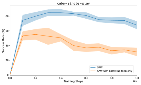
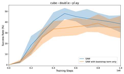
Figure 4: Training curves for cube-single-play and cube-double-play with one-step ablations.

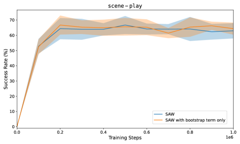
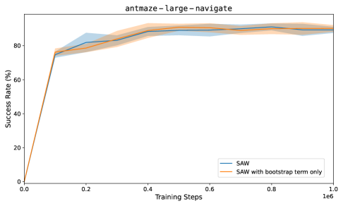
Figure 5: Training curves for scene-play and antmaze-large-navigate with one-step ablations.

H.2 Hyperparameter sensitivity

Here, we investigate SAW’s sensitivity to the $\beta$ inverse temperature hyperparameter and run different settings of $\beta\in\{0.3,1.0,3.0,10.0\}$ across selected state-based environments. We observe a similar pattern to the one-step AWR ablation experiments, where the simpler manipulation environments are much more sensitive to hyperparameter settings compared to more complex, long-horizon tasks.

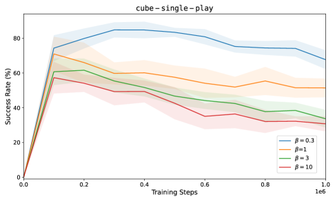
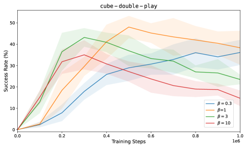
Figure 6: Training curves for cube-single-play and cube-double-play with different values of $\beta$ (where the default hyperparameters settings are $\beta=0.3$ and $\beta=1$, respectively).

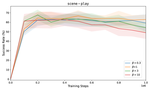
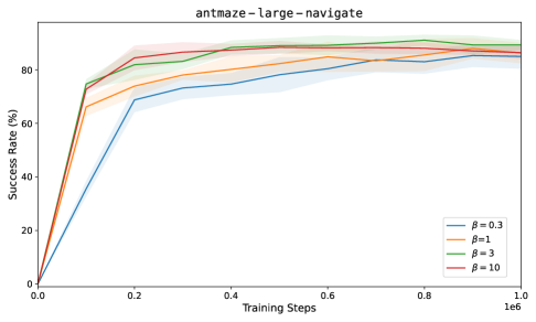
Figure 7: Training curves for scene-play and antmaze-large-navigate with different values of $\beta$ (where the default hyperparameters settings are $\beta=1$ and $\beta=3$, respectively).

References

- Abdolmaleki et al. (2018) Abdolmaleki, A., Springenberg, J. T., Tassa, Y., Munos, R., Heess, N., and Riedmiller, M. Maximum a Posteriori Policy Optimisation, June 2018. URL http://arxiv.org/abs/1806.06920. arXiv:1806.06920 [cs].
- Andrychowicz et al. (2018) Andrychowicz, M., Wolski, F., Ray, A., Schneider, J., Fong, R., Welinder, P., McGrew, B., Tobin, J., Abbeel, P., and Zaremba, W. Hindsight Experience Replay, February 2018. URL http://arxiv.org/abs/1707.01495. arXiv:1707.01495.
- Azar et al. (2017) Azar, M. G., Osband, I., and Munos, R. Minimax Regret Bounds for Reinforcement Learning. In Proceedings of the 34th International Conference on Machine Learning, pp. 263–272. PMLR, July 2017. URL https://proceedings.mlr.press/v70/azar17a.html. ISSN: 2640-3498.
- Bacon et al. (2016) Bacon, P.-L., Harb, J., and Precup, D. The Option-Critic Architecture, December 2016. URL http://arxiv.org/abs/1609.05140. arXiv:1609.05140 [cs].
- Black et al. (2024) Black, K., Brown, N., Driess, D., Esmail, A., Equi, M., Finn, C., Fusai, N., Groom, L., Hausman, K., Ichter, B., Jakubczak, S., Jones, T., Ke, L., Levine, S., Li-Bell, A., Mothukuri, M., Nair, S., Pertsch, K., Shi, L. X., Tanner, J., Vuong, Q., Walling, A., Wang, H., and Zhilinsky, U. : A Vision-Language-Action Flow Model for General Robot Control, October 2024. URL http://arxiv.org/abs/2410.24164. arXiv:2410.24164 [cs] version: 1.
- Chane-Sane et al. (2021) Chane-Sane, E., Schmid, C., and Laptev, I. Goal-Conditioned Reinforcement Learning with Imagined Subgoals. In Proceedings of the 38th International Conference on Machine Learning, pp. 1430–1440. PMLR, July 2021. URL https://proceedings.mlr.press/v139/chane-sane21a.html. ISSN: 2640-3498.
- Czechowski et al. (2024) Czechowski, K., Odrzygozdz, T., Zbysinski, M., Zawalski, M., Olejnik, K., Wu, Y., Kucinski, L., and Milos, P. Subgoal Search For Complex Reasoning Tasks, April 2024. URL http://arxiv.org/abs/2108.11204. arXiv:2108.11204.
- Dayan & Hinton (1992) Dayan, P. and Hinton, G. E. Feudal Reinforcement Learning. In Advances in Neural Information Processing Systems, volume 5. Morgan-Kaufmann, 1992. URL https://proceedings.neurips.cc/paper/1992/hash/d14220ee66aeec73c49038385428ec4c-Abstract.html.
- Eysenbach et al. (2019) Eysenbach, B., Salakhutdinov, R., and Levine, S. Search on the Replay Buffer: Bridging Planning and Reinforcement Learning, June 2019. URL http://arxiv.org/abs/1906.05253. arXiv:1906.05253 [cs].
- Eysenbach et al. (2022) Eysenbach, B., Zhang, T., Levine, S., and Salakhutdinov, R. R. Contrastive Learning as Goal-Conditioned Reinforcement Learning. Advances in Neural Information Processing Systems, 35:35603–35620, December 2022. URL https://proceedings.neurips.cc/paper_files/paper/2022/hash/e7663e974c4ee7a2b475a4775201ce1f-Abstract-Conference.html.
- Fujimoto & Gu (2021) Fujimoto, S. and Gu, S. S. A Minimalist Approach to Offline Reinforcement Learning, December 2021. URL http://arxiv.org/abs/2106.06860. arXiv:2106.06860.
- Ghosh et al. (2020) Ghosh, D., Gupta, A., Reddy, A., Fu, J., Devin, C., Eysenbach, B., and Levine, S. Learning to Reach Goals via Iterated Supervised Learning, October 2020. URL http://arxiv.org/abs/1912.06088. arXiv:1912.06088.
- Gupta et al. (2020) Gupta, A., Kumar, V., Lynch, C., Levine, S., and Hausman, K. Relay Policy Learning: Solving Long-Horizon Tasks via Imitation and Reinforcement Learning. In Proceedings of the Conference on Robot Learning, pp. 1025–1037. PMLR, May 2020. URL https://proceedings.mlr.press/v100/gupta20a.html. ISSN: 2640-3498.
- Hafner et al. (2022) Hafner, D., Lee, K.-H., Fischer, I., and Abbeel, P. Deep Hierarchical Planning from Pixels. May 2022. URL https://openreview.net/forum?id=wZk69kjy9_d.
- Hatch et al. (2024) Hatch, K. B., Balakrishna, A., Mees, O., Nair, S., Park, S., Wulfe, B., Itkina, M., Eysenbach, B., Levine, S., Kollar, T., and Burchfiel, B. GHIL-Glue: Hierarchical Control with Filtered Subgoal Images, October 2024. URL http://arxiv.org/abs/2410.20018. arXiv:2410.20018 [cs].
- Hoang et al. (2021) Hoang, C., Sohn, S., Choi, J., Carvalho, W., and Lee, H. Successor Feature Landmarks for Long-Horizon Goal-Conditioned Reinforcement Learning. In Advances in Neural Information Processing Systems, volume 34, pp. 26963–26975. Curran Associates, Inc., 2021. URL https://proceedings.neurips.cc/paper/2021/hash/e27c71957d1e6c223e0d48a165da2ee1-Abstract.html.
- Huang et al. (2019) Huang, Z., Liu, F., and Su, H. Mapping State Space using Landmarks for Universal Goal Reaching. In Advances in Neural Information Processing Systems, volume 32. Curran Associates, Inc., 2019. URL https://proceedings.neurips.cc/paper_files/paper/2019/hash/3b712de48137572f3849aabd5666a4e3-Abstract.html.
- Intelligence et al. (2025) Intelligence, P., Black, K., Brown, N., Darpinian, J., Dhabalia, K., Driess, D., Esmail, A., Equi, M., Finn, C., Fusai, N., Galliker, M. Y., Ghosh, D., Groom, L., Hausman, K., Ichter, B., Jakubczak, S., Jones, T., Ke, L., LeBlanc, D., Levine, S., Li-Bell, A., Mothukuri, M., Nair, S., Pertsch, K., Ren, A. Z., Shi, L. X., Smith, L., Springenberg, J. T., Stachowicz, K., Tanner, J., Vuong, Q., Walke, H., Walling, A., Wang, H., Yu, L., and Zhilinsky, U. : a Vision-Language-Action Model with Open-World Generalization, April 2025. URL http://arxiv.org/abs/2504.16054. arXiv:2504.16054 [cs] version: 1.
- Kaelbling (1993) Kaelbling, L. P. Learning to achieve goals. In IJCAI, volume 2, pp. 1094–8. Citeseer, 1993. URL https://citeseerx.ist.psu.edu/document?repid=rep1&type=pdf&doi=6df43f70f383007a946448122b75918e3a9d6682.
- Kostrikov et al. (2021) Kostrikov, I., Nair, A., and Levine, S. Offline Reinforcement Learning with Implicit Q-Learning. October 2021. URL https://openreview.net/forum?id=68n2s9ZJWF8.
- Lange et al. (2012) Lange, S., Gabel, T., and Riedmiller, M. Batch Reinforcement Learning. In Wiering, M. and van Otterlo, M. (eds.), Reinforcement Learning: State-of-the-Art, pp. 45–73. Springer, Berlin, Heidelberg, 2012. ISBN 978-3-642-27645-3. doi: 10.1007/978-3-642-27645-3_2. URL https://doi.org/10.1007/978-3-642-27645-3_2.
- Levine (2018) Levine, S. Reinforcement Learning and Control as Probabilistic Inference: Tutorial and Review, May 2018. URL http://arxiv.org/abs/1805.00909. arXiv:1805.00909 [cs].
- Levine et al. (2020) Levine, S., Kumar, A., Tucker, G., and Fu, J. Offline Reinforcement Learning: Tutorial, Review, and Perspectives on Open Problems, November 2020. URL http://arxiv.org/abs/2005.01643. arXiv:2005.01643.
- Levy et al. (2019) Levy, A., Konidaris, G., Platt, R., and Saenko, K. Learning Multi-Level Hierarchies with Hindsight, September 2019. URL http://arxiv.org/abs/1712.00948. arXiv:1712.00948 [cs].
- Ma et al. (2022) Ma, J. Y., Yan, J., Jayaraman, D., and Bastani, O. Offline Goal-Conditioned Reinforcement Learning via -Advantage Regression. Advances in Neural Information Processing Systems, 35:310–323, December 2022. URL https://proceedings.neurips.cc/paper_files/paper/2022/hash/022a39052abf9ca467e268923057dfc0-Abstract-Conference.html.
- Ma et al. (2023) Ma, Y. J., Sodhani, S., Jayaraman, D., Bastani, O., Kumar, V., and Zhang, A. VIP: Towards Universal Visual Reward and Representation via Value-Implicit Pre-Training, March 2023. URL http://arxiv.org/abs/2210.00030. arXiv:2210.00030 [cs].
- Myers et al. (2025) Myers, V., Ji, C., and Eysenbach, B. Horizon Generalization in Reinforcement Learning, January 2025. URL http://arxiv.org/abs/2501.02709. arXiv:2501.02709 [cs].
- Nachum et al. (2018) Nachum, O., Gu, S., Lee, H., and Levine, S. Data-Efficient Hierarchical Reinforcement Learning, October 2018. URL http://arxiv.org/abs/1805.08296. arXiv:1805.08296.
- Nachum et al. (2019) Nachum, O., Tang, H., Lu, X., Gu, S., Lee, H., and Levine, S. Why Does Hierarchy (Sometimes) Work So Well in Reinforcement Learning?, December 2019. URL http://arxiv.org/abs/1909.10618. arXiv:1909.10618 [cs].
- Nair et al. (2023) Nair, S., Rajeswaran, A., Kumar, V., Finn, C., and Gupta, A. R3M: A Universal Visual Representation for Robot Manipulation. In Proceedings of The 6th Conference on Robot Learning, pp. 892–909. PMLR, March 2023. URL https://proceedings.mlr.press/v205/nair23a.html. ISSN: 2640-3498.
- Park et al. (2024a) Park, S., Frans, K., Eysenbach, B., and Levine, S. OGBench: Benchmarking Offline Goal-Conditioned RL, October 2024a. URL http://arxiv.org/abs/2410.20092. arXiv:2410.20092.
- Park et al. (2024b) Park, S., Frans, K., Levine, S., and Kumar, A. Is Value Learning Really the Main Bottleneck in Offline RL?, October 2024b. URL http://arxiv.org/abs/2406.09329. arXiv:2406.09329.
- Park et al. (2024c) Park, S., Ghosh, D., Eysenbach, B., and Levine, S. HIQL: Offline Goal-Conditioned RL with Latent States as Actions, March 2024c. URL http://arxiv.org/abs/2307.11949. arXiv:2307.11949 [cs].
- Park et al. (2024d) Park, S., Kreiman, T., and Levine, S. Foundation Policies with Hilbert Representations, May 2024d. URL http://arxiv.org/abs/2402.15567. arXiv:2402.15567 [cs].
- Peng et al. (2019) Peng, X. B., Kumar, A., Zhang, G., and Levine, S. Advantage-Weighted Regression: Simple and Scalable Off-Policy Reinforcement Learning, October 2019. URL http://arxiv.org/abs/1910.00177. arXiv:1910.00177.
- Puterman (2005) Puterman, M. L. Markov Decision Processes: Discrete Stochastic Dynamic Programming. John Wiley and Sons, 2005.
- Schulman et al. (2017) Schulman, J., Levine, S., Moritz, P., Jordan, M. I., and Abbeel, P. Trust Region Policy Optimization, April 2017. URL http://arxiv.org/abs/1502.05477. arXiv:1502.05477 [cs].
- Seo et al. (2022) Seo, Y., Lee, K., James, S., and Abbeel, P. Reinforcement Learning with Action-Free Pre-Training from Videos, June 2022. URL http://arxiv.org/abs/2203.13880. arXiv:2203.13880 [cs].
- Stone (2008) Stone, N. K. J. a. T. H. a. P. The Utility of Temporal Abstraction in Reinforcement Learning. 2008. URL https://www.cs.utexas.edu/˜ai-lab/?AAMAS08-jong.
- Strehl et al. (2009) Strehl, A. L., Li, L., and Littman, M. L. Reinforcement Learning in Finite MDPs: PAC Analysis. Journal of Machine Learning Research, 10(84):2413–2444, 2009. ISSN 1533-7928. URL http://jmlr.org/papers/v10/strehl09a.html.
- Sutton et al. (1999) Sutton, R. S., Precup, D., and Singh, S. Between MDPs and semi-MDPs: A framework for temporal abstraction in reinforcement learning. Artificial Intelligence, 112(1):181–211, August 1999. ISSN 0004-3702. doi: 10.1016/S0004-3702(99)00052-1. URL https://www.sciencedirect.com/science/article/pii/S0004370299000521.
- Tian et al. (2020) Tian, S., Nair, S., Ebert, F., Dasari, S., Eysenbach, B., Finn, C., and Levine, S. Model-Based Visual Planning with Self-Supervised Functional Distances. October 2020. URL https://openreview.net/forum?id=UcoXdfrORC.
- Vezhnevets et al. (2017) Vezhnevets, A. S., Osindero, S., Schaul, T., Heess, N., Jaderberg, M., Silver, D., and Kavukcuoglu, K. FeUdal Networks for Hierarchical Reinforcement Learning, March 2017. URL http://arxiv.org/abs/1703.01161. arXiv:1703.01161 [cs].
- Wang et al. (2025) Wang, K., Javali, I., Bortkiewicz, M., Trzcinski, T., and Eysenbach, B. 1000 Layer Networks for Self-Supervised RL: Scaling Depth Can Enable New Goal-Reaching Capabilities, March 2025. URL http://arxiv.org/abs/2503.14858. arXiv:2503.14858 [cs].
- Wang & Isola (2022) Wang, T. and Isola, P. Understanding Contrastive Representation Learning through Alignment and Uniformity on the Hypersphere, August 2022. URL http://arxiv.org/abs/2005.10242. arXiv:2005.10242 [cs].
- Wang & Isola (2024) Wang, T. and Isola, P. Improved Representation of Asymmetrical Distances with Interval Quasimetric Embeddings, January 2024. URL http://arxiv.org/abs/2211.15120. arXiv:2211.15120 [cs].
- Wang et al. (2023) Wang, T., Torralba, A., Isola, P., and Zhang, A. Optimal Goal-Reaching Reinforcement Learning via Quasimetric Learning, November 2023. URL http://arxiv.org/abs/2304.01203. arXiv:2304.01203 [cs].
- Yang et al. (2022) Yang, R., Lu, Y., Li, W., Sun, H., Fang, M., Du, Y., Li, X., Han, L., and Zhang, C. Rethinking Goal-conditioned Supervised Learning and Its Connection to Offline RL, February 2022. URL http://arxiv.org/abs/2202.04478. arXiv:2202.04478 [cs].
- Yang et al. (2023) Yang, R., Yong, L., Ma, X., Hu, H., Zhang, C., and Zhang, T. What is Essential for Unseen Goal Generalization of Offline Goal-conditioned RL? In Proceedings of the 40th International Conference on Machine Learning, pp. 39543–39571. PMLR, July 2023. URL https://proceedings.mlr.press/v202/yang23q.html. ISSN: 2640-3498.
- Zawalski et al. (2024) Zawalski, M., Tyrolski, M., Czechowski, K., Odrzygozdz, T., Stachura, D., Piekos, P., Wu, Y., Kucinski, L., and Milos, P. Fast and Precise: Adjusting Planning Horizon with Adaptive Subgoal Search, May 2024. URL http://arxiv.org/abs/2206.00702. arXiv:2206.00702.
- Zeng et al. (2023) Zeng, Z., Zhang, C., Wang, S., and Sun, C. Goal-Conditioned Predictive Coding for Offline Reinforcement Learning. Advances in Neural Information Processing Systems, 36:25528–25548, December 2023. URL https://proceedings.neurips.cc/paper_files/paper/2023/hash/51053d7b8473df7d5a2165b2a8ee9629-Abstract-Conference.html.
- Zhang et al. (2021a) Zhang, L., Yang, G., and Stadie, B. C. World Model as a Graph: Learning Latent Landmarks for Planning. In Proceedings of the 38th International Conference on Machine Learning, pp. 12611–12620. PMLR, July 2021a. URL https://proceedings.mlr.press/v139/zhang21x.html. ISSN: 2640-3498.
- Zhang et al. (2020) Zhang, T., Guo, S., Tan, T., Hu, X., and Chen, F. Generating Adjacency-Constrained Subgoals in Hierarchical Reinforcement Learning. In Advances in Neural Information Processing Systems, volume 33, pp. 21579–21590. Curran Associates, Inc., 2020. URL https://proceedings.neurips.cc/paper/2020/hash/f5f3b8d720f34ebebceb7765e447268b-Abstract.html.
- Zhang et al. (2021b) Zhang, T., Eysenbach, B., Salakhutdinov, R., Levine, S., and Gonzalez, J. E. C-Planning: An Automatic Curriculum for Learning Goal-Reaching Tasks, October 2021b. URL http://arxiv.org/abs/2110.12080. arXiv:2110.12080 [cs].
- Zheng et al. (2024) Zheng, C., Salakhutdinov, R., and Eysenbach, B. Contrastive Difference Predictive Coding, February 2024. URL http://arxiv.org/abs/2310.20141. arXiv:2310.20141.