Anomaly Detection Based on Critical Paths for Deep Neural Networks

Abstract.

Deep neural networks (DNNs) are notoriously hard to understand and difficult to defend. Extracting representative paths (including the neuron activation values and the connections between neurons) from DNNs using software engineering approaches has recently shown to be a promising approach in interpreting the decision making process of blackbox DNNs, as the extracted paths are often effective in capturing essential features. With this in mind, this work investigates a novel approach that extracts critical paths from DNNs and subsequently applies the extracted paths for the anomaly detection task, based on the observation that outliers and adversarial inputs do not usually induce the same activation pattern on those paths as normal (in-distribution) inputs.

In our approach, we first identify critical detection paths via genetic evolution and mutation. Since different paths in a DNN often capture different features for the same target class, we ensemble detection results from multiple paths by integrating random subspace sampling and a voting mechanism. Compared with state-of-the-art methods, our experimental results suggest that our method not only outperforms them, but it is also suitable for the detection of a broad range of anomaly types with high accuracy.

1. Introduction

Deep neural networks (DNNs) have gained a great advantage over traditional machine learning methods for image classification tasks in recent years (He et al., 2016; Krizhevsky et al., 2012). However, it is well-known that DNN classifiers can be highly inaccurate (sometimes with high confidence) on test inputs from outside of the training distribution (Nguyen et al., 2015; Hendrycks and Gimpel, 2017; Lee et al., 2018). Such inputs, named anomaly samples, may arise in real-world settings either unintentionally due to external factors, or due to malicious adversaries that induce prediction errors in the DNN and disrupt the system. This phenomenon raises doubts about the application of the DNN model to safety-critical systems.

To address this problem, many efforts have been made to detect anomaly samples in DNN models (Meng and Chen, 2017; Cohen et al., 2020; Gong et al., 2019; Feinman et al., 2017; Ma et al., 2018b; Hendrycks and Gimpel, 2017; Lee et al., 2018; Ma and Liu, 2019; Hendrycks et al., 2019a; Sastry and Oore, 2020; Abdelzad et al., 2019). Among them, methods based on the features extracted from one layer or several layers of a DNN model are widely used (Feinman et al., 2017; Ma et al., 2018b; Hendrycks and Gimpel, 2017; Lee et al., 2018; Ma and Liu, 2019; Hendrycks et al., 2019a; Sastry and Oore, 2020; Abdelzad et al., 2019) for their acceptable performance and easy-to-understand decision logic. However, these methods do not usually generalize well across different types of anomaly samples because the activation values of a specific layer often depend on a specific anomaly type. Furthermore, an observation is that the features used in these methods are independent, meaning that the relationship of neurons between different layers in a DNN model is often ignored. While a DNN, which consists of neurons in multiple layers and connections among neurons in neighboring layers, can be considered as a weighted directed graph with nodes and weighted edges, and these connections form a huge set of paths from neurons of the input layer to neurons of the output layer. In the software engineering practice, it is well known that path-oriented testing is often beneficial for high-dependable testing performance of traditional software (Wang et al., 2019b). Likewise, we believe that the connections between neurons of neighboring layers could provide meaningful characterization for a DNN model’s functionality, and thus can be used as an indication for distinguishing normal and anomaly inputs.

Researchers have already attempted to exploit the idea of critical path borrowed from the classical program analysis techniques (Wang et al., 2018; Xie et al., 2022; Li et al., 2021; Zhang et al., 2020; Qiu et al., 2019), and have used this concept both in understanding the decision logic of the DNN and for the detection of adversarial attacks. For the methods that use paths in a decision logic (Wang et al., 2018; Xie et al., 2022; Qiu et al., 2019; Zhang et al., 2020) that is mostly determined by the computational flows through neurons and connections, the generated critical decision paths are usually sparse, and each path is defined for a unique decision class. Similar techniques are also used for conveying both adversarial perturbations and important semantic information in a deep learning model (Li et al., 2021). These paths, named as critical attacking paths, can be useful in understanding model behaviors in adversarial attacks.

Nevertheless, although the critical decision paths have been successfully used for detecting adversarial samples (Wang et al., 2018; Zhang et al., 2020, 2020; Qiu et al., 2019), they have not been applied in detecting other types of anomaly samples such as out-of-distribution samples and random noises. When attempting to adopt existing critical paths extraction methods in detection of various anomaly types, we observe the following limitations.

• Efficiency. The existing methods often require a significant amount of time for profiling a collection of paths according to all inputs from a given training set, before applying an abstraction operation to merge these paths for each class and/or each adversarial attack type.

• Stablility. The existing methods often target on the decision making of a specific attack, which makes the detection performance unstable across other attack types and other anomaly types.

• Application Scope. The existing critical paths approaches have not been used to detect out-of-distribution samples and noise data.

To address the limitation on efficiency, we propose a novel approach that extracts sequences of neurons, called critical detection paths, from a large volume of samples at once. In our construction, a critical detection path starts from the input layer and ends at the output layer, which contains a single neuron for each layer. Instead of selecting one critical path for each sample, in our approach, we construct a mixed set from both normal and anomaly samples, and then use the mixed set to select one critical detection path for each class, inspired by the ways of genetic evolution (Floreano and Mattiussi, 2008) and mutation (Ma et al., 2018c). Different from previous approaches for critical decision paths and critical attacking paths (Wang et al., 2018; Zhang et al., 2020, 2020; Qiu et al., 2019), our critical detection path has only one neuron for each layer, while the paths of other approaches may have several neurons for each layer. Moreover, our method generalizes well across various of anomaly samples, including different types of adversarial inputs, out-of-distribution inputs, and random noises, while the existing methods focus on detection and interpretation of adversarial inputs only. On the technical side, we extract several paths by using a random subspace algorithm (Ho, 1998), and subsequently apply a voting mechanism that combines the results of several critical detection paths to achieve a better detection accuracy.

In this paper, we propose a general purpose anomaly detection method called Anomaly Detection based on Critical Paths (ADCP). This approach is based on the observation that there is a significant difference between the distribution of normal and anomaly samples when using features on the extracted critical detection paths, as illustrated in Figure 1. Therefore, we can predict whether an arbitrary input is anomaly or not by using the features represented as a vector of activation values spanning across the associated paths.

The contributions of this work can be summarised as follows:

• We propose a novel approach that extracts critical detection paths from a DNN that are suitable for detecting adversarial (AD), out-of-distribution (OOD), and noise (NS) samples. Our critical detection paths contain a smaller number of neurons, as well as less connections between neurons.

• Based on the detection results of several critical paths, we design a novel detection method. This method improves detection accuracy and consistently performs well for different types of anomaly samples across various DNN models and datasets.

• We conduct extensive experiments to show the effectiveness of the proposed approach, analyze the results, and demonstrate the importance of critical detection paths in the detection process.

2. Problem Formulation

A target deep neural network (DNN) model denoted as $\mathit{M}$, can be represented as a function $f:\mathcal{X}\rightarrow C$ that maps each input $x\in\mathcal{X}$ to a certain class $c\in C$. Assume $\mathit{M}$ contains $N$ layers (including the input layer, the hidden layers and the output layer), and the $i$-th layer is denoted as $L_{i}\ (0\leq i\leq N-1)$. Assume there are $w_{i}$ number of neurons in the layer $L_{i}$, denoted as $n_{i}^{0},n_{i}^{1},\cdots,n_{i}^{w_{i}-1}$ respectively. Given a test input $x$, we denote the activation value of the neuron $n_{i}^{j}$ ($0\leq j\leq w_{i}-1$) as $s_{i}^{j}(x)$: when layer $i$ is a fully connected layer, $s_{i}^{j}(x)$ is the activation value; when layer $i$ is a convolutional layer, then $s_{i}^{j}(x)$ is the average pooling value of channel (kernel) $j$.

Definition 2.1.

A path of DNN model $M$ is defined as a sequence of neurons $\langle n_{0}^{v_{0}},n_{1}^{v_{1}},\ldots,n_{N-1}^{v_{N-1}}\rangle$ where

• neuron $n_{i}^{v_{i}}$ is at the $i$-th layer $L_{i}$, with $0\leq v_{i}\leq w_{i}-1$,

• neighboring neurons belong to two connected layers, i.e., if $n_{i}^{v_{i}}$ is followed by $n_{j}^{v_{j}}$ in the path, $j=i+1$.

A path is instantiated with values when a test input $x$ is given, formally, the instance of a path $\langle n_{0}^{v_{0}},n_{1}^{v_{1}},\ldots,n_{N-1}^{v_{N-1}}\rangle$ with a given input $x$ is $\langle s_{0}^{v_{0}}(x),\ldots,s_{N-1}^{v_{N-1}}(x)\rangle$.

Therefore, selecting one neuron from each layer following the order of layers will form a path. For an $N$-layer model, the length of the path is $N$, and in-total there are $w_{0}*w_{1}*\ldots*w_{N-1}$ number of paths, which is often a large number. This work aims to select a small subset of paths that could be effectively used for the purpose of anomaly detection.

Essentially the function $f$ of a model $M$ is determined based on a set of training data—a set of input $x$ each of which has a label $c_{x}$ to denote its ground-truth class. The DNN model generally obtains a generalization area of input based on the training data. If an input $x$ is outside the generalization area, we usually take it as an anomaly (Lust and Condurache, 2020). Three types of anomaly are considered in the literature depending on how they are generated: Adversarial (AD) data is generated by adding perturbation to a clean input; Out-of-Distribution (OOD) data refers to an input that are sampled from a different distribution of the training data; Noise (NS) data are random noise (e.g. Gaussian noise) and fooling images. The fooling images are created by evolving meaningless images in order to mislead a DNN to output classes with high confidence (Nguyen et al., 2015). As the literature suggests that the characteristics of each class can be captured by different set of paths, we conjunct that anomaly data requires a specific set of paths to represent, and these set of paths can be used for anomaly detection.

Support Vector Domain Description.

Our anomaly detection algorithm is based on one class classification, which has been well studied for anomaly detection tasks (Ma and Liu, 2019; Ruff et al., 2018, 2020). In our work, we use the one class classification known as Support Vector Domain Description (SVDD) by (Tax and Duin, 1999). Another important approach for one class classification known as $\nu$-SVC is introduced by Schölkopf et al. (Schölkopf et al., 2001), which can be shown as equivalent to SVDD when the Gaussian kernel is used (Tax, 2001). Similar to the famous Support Vector Machine (Vapnik, 2000), SVDD defines support vectors for a sphere shaped decision boundary enclosing the class of objects represented by the (unlabeled) training data with minimal space, as shown in the following formulation.

(1) $$\min\limits_{R,a,\xi}\ R^{2}+\frac{1}{n\nu}\sum_{i}\xi_{i}$$

$$\mbox{s.t. }\forall i:\quad\|x_{i}-a\|^{2}\leq R^{2}+\xi_{i},\quad\xi_{i}\geq 0$$

The solution of the above constraints provides a center vector $a$, radius $R$ and slack variables $\xi_{i}$ such that the target term in Eq. (1) is minimized, provided that the square of distance from each training data $x_{i}$ to the center $a$ may exceed $R^{2}$ by at most $\xi_{i}$. Here $\nu$ is a constant in $(0,1]$ and $n$ is the size of the training set. Intuitively, a smaller $\nu$ gives more weight to the right hand side of target term in Eq. (1), which imposes smaller values for $\xi_{i}$ and larger $R$. The solution of Eq. (1) allows us to determine if a test input $z$ is from the normal data by checking the following condition.

(2) $$\|z-a\|^{2}=(z\cdot z)-2\sum_{i}\alpha_{i}(z\cdot x_{i})+\sum_{i,j}\alpha_{i}\alpha_{j}(z\cdot x_{i})\leq R^{2}$$

Here $\alpha_{i}$ ($\alpha_{j}$) is the Lagrange multiplier associated with the constraint for the $i$-th ($j$-th) training input when solving Eq. (1), which is non-zero only if the $i$-th ($j$-th) training input is used as a support vector. Given all inputs (including the test input) only appearing in the form of inner product, it is thus viable to replace the inner products by kernel functions, of which the Gaussian Radial Basis Function (RBF) provides the best performance in practice (Tax, 2001). The RBF kernel is given in the following formulation, where the free parameter $s$ controls the spread, or how tight the density is, of the kernel.

(3) $$K(x_{i},x_{j})=\exp(-\|x_{i}-x_{j}\|^{2}/s^{2})$$

During production runs, we only use the training set to train SVDD and compute the probabilities for the extracted critical paths. In other words, we collect the probabilities with SVDD models across all critical paths. Given an input $x$, a standard SVDD classifier is used to calculate the probability for each critical path. We can conject whether $x$ is an anomaly sample based on these probabilities and report the results. Details are illustrated in Subsection 3.2.

3. Our Approach

In this section, we present the methodology known as Anomaly Detection based on Critical Paths (ADCP). We have conducted a preliminary study taking a LeNet model with the MNIST dataset as training (i.e., in-distribution) data, and we treat the Fashion-MNIST dataset as anomaly (out-of-distribution) data. The extracted paths features are used to separate the two datasets, with the results visualized in Figure 1. There are $10$ figures corresponding to the $10$ MNIST classes, due to that we perform the separation based on the output of the LeNet model. For example, the upper-left figure displays all data classified as class $1$ by the LeNet model, of which MNIST data are depicted in the green color and Fashion-MNIST data are all depicted in the brown color. These figures have indicated a reasonable separation of anomaly data from in-distribution samples for all of the $10$ MNIST classes.

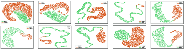
Figure 1. Two-dimensional representations of features extracted from the critical detection path of a LeNet model trained on MNIST. The feature clusters for the $10$ classes are shown, with green dots for MNIST (normal) data and brown dots for F-MNIST (anomaly) data.

Following this observation, we propose our approach in the following two phases: path extraction and anomaly detection.

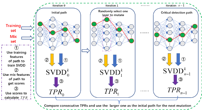
Figure 2. The overview of our approach for selecting critical detection path.

3.1. Critical Detection Path Extraction

We propose to use genetic evolution (Floreano and Mattiussi, 2008) and mutation (Ma et al., 2018c) to extract a set of paths that are used in the subsequent analysis. The entire process is shown in Figure 2, and we define a selection metric to evaluate performance of the paths, which is given in the next paragraph. At the beginning, an initial path is randomly selected. Then in the next iteration, we randomly select one layer and mutate the corresponding neuron (by randomly selecting a different neuron of the same layer). The scores before and after the mutation are compared, and if the score of the mutated path is higher, then the old path is (greedily) replaced by the new path; otherwise the old path is retained. In this way, we evolve the critical path by mutating one neuron at a time until a given number of iterations are completed.

To calculate the selection metric, each iteration consists of three procedures (see Figure 2): We use the features (neuron activation values as detailed later) of the training set on a given path of neurons to train a Support Vector Domain Description (SVDD) model. We feed the features of a mixed set of normal and anomaly samples on the same path to the pretrained SVDD model to obtain a score for each sample. We calculate the selection score for this path by integrating these individual scores. This is implemented by calculating the True Positive Positive Rate (TPR) which is often used as a metric to evaluate the performance.

(4) $$TPR=\frac{TP}{TP+FN}$$

where true positive (TP) is the number of cases when an anomaly sample is correctly reported as anomaly, and false negative (FN) is the number of cases when an anomaly is incorrectly reported as normal. The TP and FN are obtained from the individual scores by comparing with a given threshold $\tau$: for an anomaly data $x$, if its score is below the corresponding threshold $\tau$, it is reported as TP, otherwise, it is reported as FN. The threshold is different for each class, and is calculated in a way to ensure that $95\%$ of the normal samples from this class have scores above $\tau$.

As discussed in the literature, the characteristics for each decision class are different, and thus the critical detection path is different for each class. Since there is randomness in the path extraction process i.e., we randomly select the initial path, randomly select a layer to mutate, and randomly select a neuron in the layer, selecting only one path as the result may miss out other important paths. Therefore, we select multiple paths as the critical detection paths for each class (see the evaluation section for a discussion on the optimal number of paths). Since we use the same procedure to extract a critical detection path for each class, at this point, we focus on the path generation process assuming a particular class $k$ in the following paragraphs.

We first randomly select a neuron from each hidden layer to form an initial path. Then we feed all samples belonging to class $k$ from the training set into the model $\mathit{M}$ and obtain the neuron activation values for the selected neurons from these input samples. If the hidden layer is a convolutional layer, the neuron activation value is the average pooling value corresponding to the selected channel.

Next, we construct a mixed set consisting of anomaly and normal samples belonging to class $k$. The normal samples are from a test set. Note that we use different anomaly samples to form the mixed set for different types of anomaly detection tasks. In particular, for AD detection, we consider two scenarios. In one scenario, anomaly samples are a collection of adversarial samples of different attack methods. Taking into account the number of normal samples on the test set, for MNIST and CIFAR-10, we randomly select $200$ adversarial samples for each class from each attack, and for SVHN, we select 400 adversarial samples for each class from each attack. Therefore, the number of normal samples and anomaly samples is relatively close among the mixed set. In the other scenario, anomaly samples only consist of all FGSM inputs. For OOD/NS detection, we pick one OOD set as anomaly sample. For MNIST, we pick F-MNIST as anomaly set. For CIFAR-10 and SVHN, we pick TinyImageNet as anomaly set. We feed all mixed samples into $\mathit{M}$ and obtain the neuron activation values for the selected neurons from these mixed samples. Suppose the mixed set consists of $2000$ samples, the features of an initial path is a matrix of size $2000*5$ (suppose the target DNN has $5$ layers), denoted as $V_{0}^{*}$. We feed $V_{0}^{*}$ into SVDD${}_{0}^{k}$, and SVDD${}_{0}^{k}$ returns a score for each sample (corresponding to in Figure 2). Then we use these scores to calculate the True Positive Rate (TPR), donated as TPR₀ (corresponding to in Figure 2).

In the second iteration, we randomly select one layer to mutate, and the unselected layers remain unchanged. Taking the LeNet (for MNIST) as an example, assume the initial path is $\langle n_{0,1},n_{1,3},n_{2,\textbf{5}},n_{3,7},n_{4,9}\rangle$. We select the 2-nd layer to mutate, the path then becomes $\langle n_{0,1},n_{1,3},n_{2,\textbf{8}},n_{3,7},n_{4,9}\rangle$. By repeating the steps and for the mutated path in the second iteration, we can get a vector $V_{1}$ and $V_{1}^{*}$ from the training set and mixed set in separate. We use $V_{1}$ to train another SVDD model SVDD${}_{1}^{k}$ and feed $V_{1}^{*}$ into SVDD${}_{1}^{k}$, which returns a score for each sample. We use these scores to calculate another TPR, denoted as TPR₁. Then we compare TPR₀ and TPR₁, and take path with larger score as seed for the next iteration. Note that if the selected layer has just been mutated previously, we skip this iteration. Finally, a path $p_{i}$ with the highest TPR is returned as a critical detection path.

The entire approach is formalised in Algorithm 1, where the operator $Mutate(p_{i},l)$ returns a path information with higher TPR for the selected path $p_{i}$ and the selected mutated layer $l$.

Algorithm 1 Get critical detection paths

0:     $\mathit{M}$: DNN model; X_train: all samples belonging to class $k$ from the training set; X_mix: all samples belonging to class $k$ from the mixed set; $m$: the number of critical detection paths; $n$: the number of mutations;

0:     P: $m$ critical detection paths

1:  P = {}

2:  for $j=0,\cdots,m-1$ do

3:   Randomly selected one initial path $p_{0}$

4:   Calculate $TPR_{0}$

5:   LastVisit := -1

6:   for $i=0,\cdots,n-1$ do

7:    Randomly selected one layer $l$ to mutate

8:    if LastVisit $\neq l$ then

9:     $p_{i}\leftarrow Mutate(p_{0},l)$

10:     Calculate $TPR_{i}$

11:     LastVisit $=l$

12:    end if

13:    if $TPR_{i}>TPR_{0}$ then

14:     $p_{0}=p_{i}$

15:     $TPR_{0}=TPR_{i}$

16:    end if

17:   end for

18:   P $\leftarrow$ [P; $p_{0}$]

19:  end for

20:  return  P

3.2. Anomaly Detection

Based on the selected critical detection paths, we design a novel approach to detect anomaly samples by using the random subspace algorithm (Ho, 1998) and a voting mechanism.

First, we sort the critical detection paths represented as a sequence of $TPR$s in descending order. Then we feed all the samples of each class in the training set into $\mathit{M}$ in separate, and extract the features of the corresponding critical detection paths. Taking class $k$ as an example, if there are $m$ critical detection paths, we can get $m$ vectors, denoted as $V_{1},V_{2},\cdots,V_{m}$. Then we use each $V_{i}\ (1\leq i\leq m)$ to train an SVDD model and we finally obtain $m$ SVDD models for class $k$, denoted as SVDD₁, SVDD${}_{2},\cdots,$ SVDD_m. Taking the LeNet (for MNIST) as an example, in-total, we get $m\times 10$ SVDD models ($10$ classes), denoted as SVDD${}_{i}^{j}$, where $1\leq i\leq m$ and $0\leq j\leq 9$. These SVDD models are used in the following anomaly detection procedure.

Given a test data, first, we run $\mathit{M}$ to obtain a predicted class $k$. Then, we extract the features of the corresponding critical detection paths as $V_{i}^{{}^{\prime}}\ (1\leq i\leq m)$. $V_{i}^{{}^{\prime}}$ is forwarded to the pretrained model SVDD${}_{i}^{k}$ to get a score. For $m$ critical detection paths, we obtain $m$ scores. As different critical paths tend to generate scores at different scales, we apply the min-max normalization procedure.

(5) $$score_{i}^{*}=\frac{score_{i}-score_{min}}{score_{max}-score_{min}}$$

where the $score_{min}$ and $score_{max}$ are the minimum and maximum of the score vector, respectively.

For each critical detection path, we set a threshold $\tau$ for each class in advance. The threshold is the same as described in subsection 3.1. We initialize two sets $A$ and $B$ to save scores in separate. If the score is above the threshold, the score is saved to $A$, and if it is below the threshold, the score is saved to $B$. The final score is calculated using a voting mechanism based on $A$ and $B$ as follows:

• If there are $m$ values in $A$, it means that the given test data is decided as a normal sample for all critical detection paths. The final score is the maximum score among all the scores in $A$.

• If there are $m$ values in $B$, it means that the test data is decided as an anomaly sample for all critical detection paths. The final score is the minimum value in $B$.

• If there are $m^{{}^{\prime}}$ values in $A$ and $m-m^{{}^{\prime}}$ values in $B$, we use a voting mechanism to decide the score. If $m^{{}^{\prime}}>m-m^{{}^{\prime}}$, we take the median value in $A$ as the final score, otherwise, we take the median value in $B$.

Threshold.

Once a final score for the test data is obtained, we use it to decide whether the input is normal or anomaly. Similar to existing methods (Hendrycks and Gimpel, 2017; Liang et al., 2018; Hsu et al., 2020), we achieve this by setting thresholds. Different from most other works, we define multiple thresholds based on classes of training samples. In the case of MNIST, there are $10$ classes of training data, so we define a threshold for each class. When a sample $x$ is given to the target DNN model which generates output class $i$, our approach collects features from each critical path for the corresponding SVDD to generate score. Then we utilize the scores of $21$ critical paths to get the final $score$ to compare with $\tau_{i}$. The threshold $\tau_{i}$ is computed in the same way while it need ensure that $95\%$ of the normal samples from class $i$ of test sets have scores above $\tau_{i}$. The threshold-based discriminator can be formally described as follows.

(6) $$isAnomaly(x)=\left\{\begin{aligned} &True,\;\;\;if\;\;score<\tau_{i}\\ &Fasle,\;\;\;if\;\;score\geq\tau_{i}\end{aligned}\right.$$

4. Evaluations

We aim to investigate and answer the following research questions through our experiments:

• RQ1: Does Algorithm 1 generate critical paths that have significantly better performance than initial paths?

• RQ2: How effective is ADCP compared with state-of-the-art anomaly detection methods?

• RQ3: Does ADCP have better performance in anomaly detection than the existing path-based approaches?

• RQ4: How does ADCP perform in terms of different hyper-parameters?

4.1. Experiment Setup

Hardware and software. We conducted our experiments on two different platforms. One is Windows $10$ desktop equipped with Intel I7-9700 $3.0$GHz processor, $16$G RAM and Nvidia GetForce GTX1660Ti. The other one is Linux equipped with Intel(R) Xeon(R) Gold 6230 $2.10$GHz processor, $64$G RAM and Nvidia Titan RTX 24G. We have implemented the experiments based on the Keras framework. We conduct experiment on three types of target DNN models, with three data sets chosen as normal samples, against various types of AD, OOD and NS data sets. Our testing code is publicly available at https://github.com/fangzhenzhao/ADCP.

Datasets and models. We evaluated our approach (ADCP) on the following well-known image classification datasets and models (see Table 1).

Table 1. The datasets and models of our work.

Dataset	Model	Accuracy on Test Dataset
MNIST	LeNet	99.20%
CIFAR-10	VGG16	93.47%
	ResNet44	91.65%
SVHN	VGG16	95.56%
	ResNet20	96.12%

Anomaly samples. We generate three types of anomaly:

• AD: We generate the adversarial attacks by using the open-source CleverHans library (Papernot et al., 2018) on TensorFlow. The adversarial attacks used in our experiments include FGSM (Goodfellow et al., 2015), PGD (Meng and Chen, 2017), JSMA (Papernot et al., 2016), DeepFool (Moosavi-Dezfooli et al., 2016) and CW (Carlini and Wagner, 2017).

• OOD: For MNIST, the OOD sets are Fashion-MNIST (F-MNIST) (Xiao et al., 2017) and Omniglot (Lake et al., 2015). For CIFAR-10, the OOD sets are TinyImageNet (Deng et al., 2009), LSUN (Yu et al., 2015), iSUN (Xu et al., 2015) and SVHN (Netzer et al., 2011). For SVHN, the OOD sets are TinyImageNet, LSUN, iSUN and CIFAR-10.

• NS: We prepare three types of noise images, namely Gaussian Noise, Uniform Noise and Fooling Image (Nguyen et al., 2015).

Metrics. We adopt two commonly used metrics, True Negative Rate at $95\%$ of True Positive Rate (TPR at $95\%$ TNR) and Area Under the Receiver Operating Characteristic curve (AUROC), to evaluate the effectiveness of our method.

4.2. RQ1: Comparison with Initial Paths

We answer RQ1 by comparing the AUROC of different paths. A highest TPR among selected $m$ initial path (Initial in Figure 3), and a path with the highest TPR among the selected $m$ critical detection paths—our approach (Critical in Figure 3) are applied to different types of anomaly samples. The experimental results are shown in Figure 3.

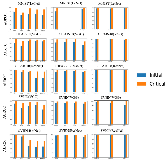
Figure 3. The AUROC corresponding to different paths on five models for different anomaly samples.

It can be seen from Figure 3 that the AUROC of the Critical path are significantly better than the Initial path for AD and OOD detection tasks. For the NS detection task, the advantage of the critical paths is not obvious in some cases, e.g. the difference is insignificant for Gaussian noises and Uniform noises in all models with CIFAR-10 and SVHN as in-distribution data.

Answer to RQ1: Our critical detection path is more effective than the initial path (highest TPR among the initial paths $m$) for detecting various types of anomaly samples.

4.3. RQ2: Comparison with Other Anomaly Detection Methods

We answer RQ2 by comparing the performance of our approach with the traditional adversarial detection approaches.

Baseline Methods

Existing amonaly detection works mostly focus on detecting either OOD or AD only. Therefore, we compare our results on OOD and NS data with models designed for OOD detection, and compare our results on AD data with models designed for adversarial attack detection, in separate. For AD detection, the baseline methods are: Local Intrinsic Dimensionality (LID) (Ma et al., 2018b), Mahalanobis Distance (MD) (Lee et al., 2018), MagNet (Meng and Chen, 2017), Feature Squeezing (FS) (Xu et al., 2018), Neural-network Invariant Checking (NIC) (Ma and Liu, 2019), Anomaly Detection based on Critical Layers (ADCL) (Zhao et al., 2022). For OOD/NS detection, the baselines are: Memory AutoEncoder (MemAE) (Gong et al., 2019), Max-Softmax (MS) (Hendrycks and Gimpel, 2017), Out-of-DIstribution detector for Neural networks (ODIN) (Liang et al., 2018), Mahalanobis Distance (MD) (Lee et al., 2018), Early Layer Output (ELO) (Abdelzad et al., 2019), and Anomaly Detection based on Critical Layers (ADCL) (Zhao et al., 2022). These methods are detailed in Section 5.

AD Detection

Among existing detecting AD data approaches, LID and MD need adversarial samples to train the detectors. However, in practice, we do not usually know whether the test data is clean or adversarial, let alone what kind of adversarial sample it is. Therefore, for a valid comparison, we make the following settings for LID and MD. For MD, we do not test MD with feature ensemble which uses the outputs from all layers and involves tuning with particular anomaly samples. We only apply the version of MD which uses the logit layer of $\mathit{M}$ instead, which have been used in the literature (Ren et al., 2019; Abdelzad et al., 2019). For LID, we use two different adversarial samples for training. The first is by only using FGSM sample as adversarial inputs, the second is by a sample mixed with all different types of adversarial inputs used in this paper, with resulting detectors called LID^∗ and (non-annotated) LID, respectively. For fair comparison between LID and ADCP, we also use two types of adversarial samples to train ADCP^∗and ADCP, so that their results are compared with their corresponding LID^∗ and LID detectors, with results shown in Table 2.

Table 2. Comparison of our approach with LID, MD, MagNet, FS and NIC for different attack on various models and datasets. Top 2 are highlighted with bold and underline.

Model	Attack	TPR at 95% TNR $\uparrow$	AUROC $\uparrow$
		LID∗ / LID / MD / MagNet / FS / NIC / ADCP∗ / ADCP
LeNet (MNIST)	FGSM	64.98/59.51/83.85/30.23/98.67/49.68/99.96/93.99	94.12/93.29/96.82/88.56/99.55/88.03/99.93/98.99
	PGD	30.38/38.43/20.82/ 8.46/99.67/15.81/65.09/76.19	83.87/85.82/77.71/66.38/99.92/71.06/91.98/97.76
	JSMA	80.91/86.35/89.95/24.09/99.79/70.18/89.85/94.12	96.54/97.47/97.82/82.78/99.33/93.87/98.08/98.81
	CW	67.64/72.89/66.33/ 5.54/100.0/30.42/57.47/82.82	94.20/95.75/95.12/60.66/99.36/84.20/93.80/97.24
	DeepFool	62.57/70.55/66.58/ 5.69/100.0/33.05/60.63/85.43	93.75/95.50/95.29/62.40/99.47/86.95/93.96/97.44
VGG (CIFAR-10)	FGSM	44.04/ 8.95/53.08/ 5.03/ 1.49/53.53/100.0/99.65	88.30/70.20/90.07/52.18/64.18/87.26/99.96/99.56
	PGD	11.56/15.72/ 5.83/ 4.61/14.60/20.15/72.11/82.34	66.97/67.71/80.40/49.78/63.11/73.24/94.54/96.57
	JSMA	17.17/60.73/97.13/ 5.24/ 0.17/71.32/92.44/97.46	69.04/93.81/98.78/51.21/63.96/93.56/98.52/99.15
	CW	0.0  /45.66/86.22/ 6.27/ 0.0  /82.60/83.35/94.92	29.41/88.60/96.96/54.17/51.59/96.30/96.68/98.97
	DeepFool	0.0  /46.87/81.07/ 6.43/ 0.0  /82.04/79.23/92.42	30.01/87.77/96.18/54.30/51.43/96.18/95.86/98.54
ResNet (CIFAR-10)	FGSM	99.94/70.33/37.69/ 4.40/ 4.53/48.68/100.0/100.0	99.97/93.33/87.33/50.31/70.61/86.47/99.95/99.93
	PGD	0.0  /70.01/85.07/ 4.42/14.18/24.07/93.38/99.53	47.81/92.41/95.87/49.43/59.83/71.55/98.40/99.76
	JSMA	14.86/70.01/35.25/ 9.78/ 1.16/69.94/88.80/94.15	62.23/92.57/92.18/62.47/71.87/93.04/96.79/98.42
	CW	0.0  /57.36/ 9.74/ 6.69/ 0.0  /32.86/30.86/85.04	38.17/92.85/82.99/54.67/52.88/78.42/84.91/97.63
	DeepFool	0.0  /61.70/ 8.74/ 6.55/ 0.0  /32.70/30.62/84.66	38.13/93.04/82.46/54.63/53.89/77.89/84.43/97.53
VGG (SVHN)	FGSM	97.57/77.28/81.58/76.52/75.67/80.60/100.0/100.0	99.41/96.11/96.49/97.36/95.82/95.99/99.98/99.93
	PGD	24.99/34.17/ 2.96/58.38/ 2.79/30.21/85.78/89.75	81.52/82.32/80.03/92.17/37.52/78.16/97.16/97.88
	JSMA	36.51/72.29/93.81/70.79/96.46/49.08/81.98/95.34	85.88/95.33/98.52/94.53/99.07/85.40/96.36/98.67
	CW	16.16/73.34/100.0/19.91/98.68/24.05/88.02/99.70	77.99/95.40/98.48/81.19/99.04/72.97/97.88/99.55
	DeepFool	27.60/55.67/67.90/42.97/75.07/30.67/61.79/81.50	79.64/90.65/92.59/87.96/95.05/78.23/89.85/94.48
ResNet (SVHN)	FGSM	98.74/75.89/68.41/77.18/83.91/54.83/100.0/100.0	99.40/95.67/94.71/98.55/97.14/89.84/99.98/99.90
	PGD	61.97/77.30/98.24/96.66/ 6.80/21.41/96.09/99.29	93.20/95.92/99.61/99.23/27.04/76.74/99.12/99.71
	JSMA	34.91/65.79/84.16/69.56/99.02/15.99/25.74/68.70	83.33/94.13/97.07/93.44/99.51/67.52/80.55/92.53
	CW	13.68/73.89/78.72/11.51/96.63/  6.46/17.62/59.63	72.94/95.52/96.68/66.82/98.38/53.11/79.81/91.12
	DeepFool	15.55/65.93/82.18/18.16/98.27/ 6.43/17.47/58.56	74.15/94.25/96.87/73.99/98.80/54.08/79.11/90.82

From the Table 2, one can observe that ADCP has the best performance $11$ times out of $25$ and is the second best $8$ times out of $25$. More importantly, for the rest cases where other methods have better precision, our results are not much behind. Noted that although the critical detection paths selected by FGSM are used for the detection of AD samples, the results generalize well over non-FGSM adversarial inputs. Compared with LID that also uses only FGSM to train the detector, our results are significantly better.

OOD/NS Detection

Similar to existing works (Lee et al., 2018; Liang et al., 2018; Abdelzad et al., 2019; Zhao et al., 2022), we apply the same training procedure for both OOD and NS detection tasks. For all these approaches, we use the same settings as the original works for a fair comparison. The experimental results of our approach and the compared methods are shown in Table 3 (OOD detection) and Table 4 (NS detection).

Table 3. Comparison of our approach with MemAE, MS, ODIN, MD, ELO and ADCL for different OOD on various models and datasets. Top 2 are highlighted with bold and underline.

Model	OOD	TPR at 95% TNR $\uparrow$	AUROC $\uparrow$
		MemAE / MS / ODIN / MD / ELO / ADCL / ADCP
LeNet (MNIST)	F-MNIST	82.20/97.90/99.59/95.60/99.16/99.76/99.99	93.89/99.26/99.81/98.81/99.77/99.85/99.97
	Omniglot	100.0/97.03/99.86/93.62/100.0/100.0/100.0	100.0/98.82/ 99.81/98.48/100.0/99.99/100.0
VGG (CIFAR-10)	TinyIm	32.90/36.14/55.76/46.61/84.96/90.35/98.21	78.03/89.79/92.79/90.68/96.51/98.23/99.33
	LSUN	38.12/38.82/63.41/56.92/92.13/95.77/99.60	81.98/90.90/94.58/93.05/98.17/99.33/99.71
	iSUN	30.15/39.06/63.65/54.90/89.39/95.96/99.34	75.33/90.89/94.53/92.61/97.82/99.08/99.59
	SVHN	1.62/27.89/43.58/23.28/87.77/73.26/90.69	28.15/89.01/91.92/85.56/97.22/96.71/97.82
ResNet (CIFAR-10)	TinyIm	29.03/30.32/48.41/15.52/95.08/94.97/99.33	78.69/87.13/90.58/79.46/98.93/98.81/99.76
	LSUN	31.18/35.47/67.04/22.84/96.21/97.73/99.23	83.17/89.66/94.72/85.22/99.08/99.37/99.82
	iSUN	24.39/34.25/63.47/22.45/93.61/96.09/98.89	78.21/89.22/94.10/84.41/98.65/99.15/99.74
	SVHN	1.35/38.71/67.27/24.77/85.29/86.99/91.16	23.74/89.74/93.80/82.19/96.78/97.38/97.96
VGG (SVHN)	TinyIm	43.93/78.69/88.79/76.37/92.15/95.57/99.98	90.21/96.92/97.99/96.56/98.23/99.15/99.95
	LSUN	47.73/78.27/88.13/78.42/93.71/96.29/99.96	92.16/96.80/97.83/96.71/98.40/99.32/99.94
	iSUN	44.15/81.48/90.83/79.82/93.65/96.90/99.92	90.08/97.26/98.27/96.95/98.48/99.35/99.93
	CIFAR-10	33.00/78.13/88.87/76.39/72.24/90.19/99.56	83.47/97.67/97.91/85.69/94.67/98.28/99.75
ResNet (SVHN)	TinyIm	65.45/75.38/85.39/63.93/93.85/96.64/99.88	92.14/96.21/97.17/94.37/98.65/99.17/99.84
	LSUN	71.54/72.67/83.02/58.96/96.34/97.46/99.94	94.30/95.85/96.72/93.64/99.09/99.33/99.86
	iSUN	63.26/75.65/86.39/63.04/95.80/97.57/99.90	92.25/96.28/97.30/94.20/99.01/99.35/99.86
	CIFAR-10	43.24/74.12/85.12/63.91/80.38/89.70/97.90	85.39/96.04/97.07/94.47/95.41/97.77/99.30

Table 4. Comparison of our approach with MemAE, MS, ODIN, MD, ELO and ADCL for different NS on various models and datasets. Top 2 are highlighted with bold and underline.

Model	NS	TPR at 95% TNR $\uparrow$	AUROC $\uparrow$
		MemAE / MS / ODIN / MD / ELO / ADCL / ADCP
LeNet (MNIST)	Gaussian	100.0/100.0/100.0/100.0/100.0/100.0/100.0	100.0/99.58/100.0/99.77/100.0/100.0/100.0
	Uniform	100.0/99.27/100.0/99.25/100.0/100.0/100.0	100.0/98.31/99.92/98.85/100.0/100.0/100.0
	FoolIm	100.0/ 0.0  / 0.0  / 2.07/100.0/100.0/98.77	100.0/75.56/86.73/68.61/100.0/99.80/99.62
VGG (CIFAR-10)	Gaussian	100.0/ 7.75/58.42/97.43/100.0/100.0/100.0	100.0/90.26/95.21/98.83/100.0/100.0/100.0
	Uniform	100.0/49.56/87.79/99.81/100.0/100.0/100.0	99.91/94.72/96.78/99.28/100.0/100.0/100.0
	FoolIm	77.55/ 0.0  / 0.0  / 0.0  /100.0/99.54/100.0	7.05/71.60/79.53/71.82/100.0/98.85/99.89
ResNet (CIFAR-10)	Gaussian	100.0/30.22/58.51/33.67/100.0/100.0/100.0	99.98/89.08/93.90/89.87/100.0/99.77/100.0
	Uniform	100.0/24.56/53.40/23.48/100.0/100.0/100.0	99.68/87.96/93.38/89.13/100.0/99.83/100.0
	FoolIm	100.0/ 0.0  / 0.0  /16.83/100.0/100.0/100.0	100.0/72.84/82.74/76.65/100.0/99.78/100.0
VGG (SVHN)	Gaussian	100.0/84.76/91.95/80.21/100.0/99.85/100.0	99.73/97.67/98.49/97.00/99.94/99.81/100.0
	Uniform	47.31/90.49/96.35/83.88/100.0/99.66/100.0	96.38/98.35/99.11/97.30/99.85/99.77/99.99
	FoolIm	99.88/ 0.0  / 0.0  / 0.0  /100.0/100.0/100.0	99.26/16.65/19.45/37.91/99.89/99.01/99.96
ResNet (SVHN)	Gaussian	100.0/83.52/93.28/66.61/100.0/100.0/100.0	99.81/97.28/98.32/95.31/99.99/99.94/99.99
	Uniform	91.76/82.68/93.08/62.76/100.0/99.99/100.0	98.28/97.28/98.32/94.89/99.93/99.90/99.96
	FoolIm	100.0/ 0.0  / 0.0  / 1.30/100.0/98.78/100.0	99.71/42.09/46.74 /53.18/99.99/98.90/99.99

From the Table 3 and Table 4, we can observe that the performance of our approach is mostly better than other methods for OOD and NS detection task. For the OOD detection tasks (Table 3), our method has the best precision in all OOD cases. For the NS detection tasks (Table 4), our method has the best precision for detection of NS anomalies in most cases. Even for the some cases when ELO is better, the percentage difference is minor.

Answer to RQ2: Compared with the state-of-the-art traditional anomaly detection methods, our approach provides more stable detection performance for AD and superior performance for OOD and NS data.

4.4. RQ3: Comparison with Other Path Extraction Methods

We answer RQ3 by comparing our approach with two other path extraction based approaches, Neuron Path Coverage (NPC) (Xie et al., 2022) and Effective Path (EffPath) (Qiu et al., 2019). We first follow their approaches to obtain critical ‘paths’ (their ‘path’ contains several neurons for each layer) from the training set, and then merge their ‘paths’ for each class to obtain the final critical decision ‘paths’. We define these two critical decision ‘paths’ as Path_NPC and Path_EffPath, respectively. Note that their ‘paths’ are defined differently from ours, and for a fair comparison, we randomly extract $21$ paths (in our definition) where one neuron per layer from Path_NPC and Path_EffPath, and denoted them as Path${}_{NPC}^{*}$ and Path${}_{EffPath}^{*}$. We show two experimental results of the EffPath method: the comparison with their original detection method using the similarity calculation, denoted as EffPath and the comparison using our approach by calculating scores using SVDD and Path${}_{EffPath}^{*}$, donated as EffPath^∗. For NPC, since their work does not apply effective paths for anomaly detection, the result is obtained by using our detection approach i.e., SVDD and Path${}_{NPC}^{*}$. These experimental results for the detection of AD, OOD and NS anomalies are shown in Table 5, Table 6 and Table 7, respectively.

Table 5. Comparison of our approach with NPC and EffPath for different attack on various models and datasets. The highest are highlighted with bold.

Model	Attack	TPR at 95% TNR $\uparrow$	AUROC $\uparrow$
		NPC / EffPath / EffPath∗ / ADCP
LeNet (MNIST)	FGSM	97.13/64.14/95.10/93.99	99.40/92.84/99.14/98.99
	PGD	45.39/35.59/46.21/76.19	88.49/83.72/90.37/97.76
	JSMA	92.60/89.77/92.91/94.12	98.56/98.01/98.57/98.81
	CW	67.32/77.34/68.36/82.82	95.47/96.08/95.39/97.24
	DeepFool	71.84/76.70/72.85/85.43	95.98/95.83/95.82/97.44
VGG (CIFAR-10)	FGSM	55.26/44.82/59.00/99.65	92.27/81.74/93.64/99.56
	PGD	40.64/71.20/45.96/82.34	86.94/94.75/89.32/96.57
	JSMA	95.92/93.47/95.66/97.46	98.84/98.71/98.95/99.15
	CW	90.10/77.71/88.07/94.92	97.51/94.62/97.34/98.97
	DeepFool	85.01/72.58/82.80/92.42	96.55/92.62/96.26/98.54
ResNet (CIFAR-10)	FGSM	99.91/  8.28/99.95/100.0	99.73/72.91/99.83/100.0
	PGD	92.31/29.11/93.25/99.53	98.16/79.09/98.34/99.76
	JSMA	89.31/79.89/88.91/94.15	96.93/95.86/96.95/98.42
	CW	34.54/38.59/33.24/85.04	85.92/86.72/85.58/97.63
	DeepFool	33.94/40.64/33.13/84.66	85.81/87.57/85.37/97.53
VGG (SVHN)	FGSM	96.51/68.29/98.05/100.0	99.38/92.26/99.43/99.93
	PGD	74.84/50.16/76.36/89.75	94.46/84.42/95.00/97.88
	JSMA	79.71/88.44/82.36/95.34	95.68/97.08/96.21/98.67
	CW	86.28/96.64/90.23/99.70	97.72/98.39/98.22/99.55
	DeepFool	54.08/63.90/57.55/81.50	87.23/88.87/88.11/94.48
ResNet (SVHN)	FGSM	100.0/61.19/100.0/100.0	99.81/91.16/99.82/99.90
	PGD	93.32/43.89/91.30/99.29	98.81/81.29/98.47/99.71
	JSMA	22.39/64.35/22.82/68.70	79.11//97.72/79.12/92.53
	CW	16.86/52.03/17.33/59.63	79.44/88.79/79.67/91.12
	DeepFool	16.98/52.85/17.16/58.56	78.93/89.54/78.99/90.82

Table 6. Comparison of our approach with NPC and EffPath for different OOD on various models and datasets. The highest are highlighted with bold.

Model	OOD	TPR at 95% TNR $\uparrow$	AUROC $\uparrow$
		NPC / EffPath / EffPath∗ / ADCP
LeNet (MNIST)	F-MNIST	98.56/88.46/99.03/99.99	99.51/97.61/99.65/99.97
	Omniglot	99.61/64.38/100.0/100.0	99.91/94.83/100.0/100.0
VGG (CIFAR-10)	TinyIm	81.69/53.60/80.53/98.21	95.76/83.01/95.94/99.33
	LSUN	90.16/60.66/89.73/99.60	98.03/87.04/98.19/99.71
	iSUN	90.90/50.01/89.89/99.34	97.67/86.22/97.86/99.59
	SVHN	65.00/26.05/68.00/90.69	94.73/78.06/95.36/97.82
ResNet (CIFAR-10)	TinyIm	87.83/44.90/87.98/99.33	97.70/85.41/97.77/99.76
	LSUN	93.19/54.41/93.35/99.23	98.66/90.33/98.67/99.82
	iSUN	90.48/49.93/90.60/98.89	98.16/88.40/98.24/99.74
	SVHN	89.17/31.27/88.76/91.16	97.31/79.18/97.22/97.96
VGG (SVHN)	TinyIm	97.03/71.72/96.76/99.98	99.44/88.89/99.42/99.95
	LSUN	97.81/74.10/97.81/99.96	99.57/90.97/99.60/99.94
	iSUN	97.95/77.34/97.86/99.92	99.55/91.58/99.56/99.93
	CIFAR-10	92.70/74.43/92.29/99.56	98.79/90.26/98.70/99.75
ResNet (SVHN)	TinyIm	97.81/71.38/98.08/99.88	99.41/88.53/99.42/99.84
	LSUN	98.86/70.37/99.04/99.94	99.62/88.81/99.64/99.86
	iSUN	98.71/71.76/98.90/99.90	99.57/88.81/99.59/99.86
	CIFAR-10	91.87/71.27/92.65/97.90	98.11/88.54/98.27/99.30

Table 7. Comparison of our approach with NPC and EffPath for different NS on various models and datasets. The highest are highlighted with bold.

Model	NS	TPR at 95% TNR $\uparrow$	AUROC $\uparrow$
		NPC / EffPath / EffPath∗ / ADCP
LeNet (MNIST)	Gaussian	100.0/71.40/100.0/100.0	100.0/95.68/100.0/100.0
	Uniform	100.0/11.15/100.0/100.0	100.0/69.53/100.0/100.0
	FoolIm	100.0/  8.47/100.0/98.77	99.97/54.37/99.95/99.62
VGG (CIFAR-10)	Gaussian	79.47/100.0/100.0/100.0	99.99/95.71/100.0/100.0
	Uniform	100.0/98.21/100.0/100.0	99.99/99.25/100.0/100.0
	FoolIm	100.0/ 0.04/100.0/100.0	99.38/48.39/99.60/99.89
ResNet (CIFAR-10)	Gaussian	100.0/82.18/100.0/100.0	100.0/93.46/100.0/100.0
	Uniform	100.0/63.26/100.0/100.0	100.0/93.22/100.0/100.0
	FoolIm	100.0/ 0.08/100.0/100.0	100.0/41.66/100.0/100.0
VGG (SVHN)	Gaussian	100.0/59.15/100.0/100.0	99.99/89.01/99.99/100.0
	Uniform	100.0/69.58/100.0/100.0	99.98/90.89/99.97/99.99
	FoolIm	100.0/ 2.99/100.0/100.0	99.88/48.54/99.90/99.96
ResNet (SVHN)	Gaussian	100.0/88.92/100.0/100.0	99.97/98.03/99.97/99.99
	Uniform	100.0/89.14/100.0/100.0	99.91/97.96/99.91/99.96
	FoolIm	100.0/ 0.18/100.0/100.0	99.96/42.98/99.94/99.99

From Table 5, Table 6 and Table 7, one can observe that when applied to the anomaly detection task, paths extracted using our approach are obviously superior to paths extracted using other approaches. In addition, the EffPath detection approach that uses the measure of similarity to detect anomaly samples, are not effective for OOD detection and invalid for Fooling images detection (see the results of Effpath in Table 6 and Table 7). This is because the paths extracted in their approach are obtained according to the predicted probability. When the predicted probability of an anomaly sample is close to the normal samples, the path extracted is the same as the path extracted from normal samples, which is not conducive in the anomaly detection task.

Answer to RQ3: Our critical detection paths outperform other critical decision paths approaches for the anomaly detection task.

4.5. The Setting of Hyper-parameters

We answer RQ4 by discussing the optimal set up of the two input parameters in the Algorithm 1: the number of mutations $n$ and the number of critical detection paths $m$.

The Number of Mutations

We conduct an experiment to study the relationship between the number of mutations applied and the TPRs during the path generation, in order to find a reasonably small $n$ which still guarantees close to optimal performance. To this end, we assign parameter $n=5000$, and show the variation of TPRs for different models (see Figure 4 for AD detection and Figure 5 for OOD detection).

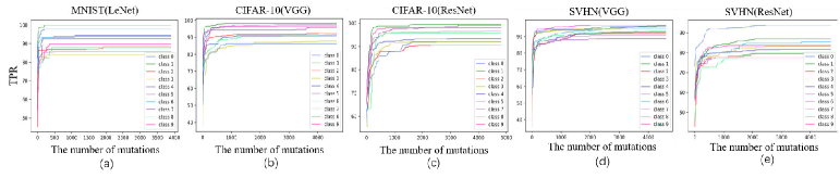
Figure 4. The TPR corresponding to the mutation number of ADCP on different models for adversarial attack in each class.

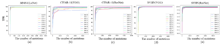
Figure 5. The TPR corresponding to the mutation number of ADCP on different models for OOD in each class.

From the Figure 4 and Figure 5, we can draw three conclusions. First, for all models, the TPRs become stable within $5000$ iterations, meaning that setting $n=5000$ ensures that the identified critical detection path is representative. Second, the TPR tends to stabilize faster on OOD than AD for a DNN model. Third, the TPRs of critical detection paths for different classes of a model are often different.

The Number of Paths

Plainly, applying more critical detection paths often yields better performance with the cost of more execution time. Hence we study the relationship between the number of paths and the detection results. The results for AD an OOD/NS detection are shown in Figure 6 and Figure 7, respectively.

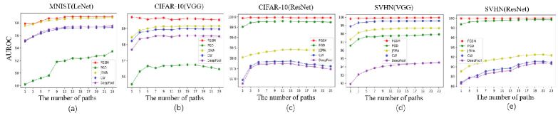
Figure 6. The AUROC corresponding to the number of paths on different models for different adversarial attacks.

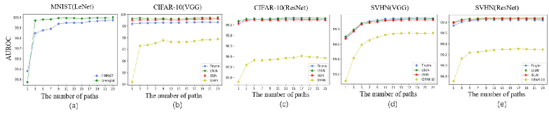
Figure 7. The AUROC corresponding to the number of paths on different models for different OOD data.

From the Figure 6 and Figure 7, we can observe that as the number of critical paths increases, the detection results first gradually increase to a certain level, and then they tend to remain stable. Especially when the number of critical detection paths increases from 1 to 3, the detection results of most anomaly samples increase significantly. After we reach the stage of $3$ paths, the performance increase tends to slow down. From the current results, the ensemble from $21$ critical detection paths seem to guarantee reasonably good detection rates for all anomaly types in the experiment.

Answer to RQ4: The parameter setup in the experiments—the mutation number set to 5000 and the path number set to 21, is reasonable.

4.6. Analysis of Each Individual Critical Detection Path

We conduct experiments to analyze the importance of each path in the detection. Taking the LeNet model with the PGD attack as an example, we study the anomaly samples (PGD) detected using three different critical paths with the highest TPRs. The results is partially visualized (for one decision class only) in Figure 8, which shows the indices of the TN outputs of the three critical paths. In the figure, the gray points represent the PGD adversarial input that can be detected correctly by all the three paths; the red points represent the inputs that can be additionally detected by path0, the green points are the inputs that can be further detected by path1, and the blue points are inputs that are further detected by path2.

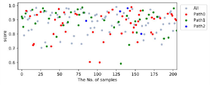
Figure 8. The visualization of 205 samples correctly decided corresponding to Top 3 critical detection paths for PGD (class 3) on MNIST.

We can observe that a majority of the PGD inputs can be detected by all three paths. However, each individual path can detect a small set of extra anomaly inputs. This indicates that combining multiple paths can improve detection performance.

4.7. Pearson Coefficient of Critical Detection Paths for Different Anomaly Samples

As shown the Figure 6 and Figure 7, the magnitude of performance improvements is obviously different for different anomaly samples. Therefore, we investigate the characteristics of their corresponding critical detection paths that lead to this phenomenon. In theory, if two paths are closely correlated, i.e., with high the Pearson coefficient, the performance cannot benefit much by combining these two paths. Hence, we conduct experiments to show the differences of their critical detection paths (in terms of Pearson coefficient) with different anomaly samples. We select $10$ paths whose TPRs are the top $10$ among the $m$ critical detection paths and take the FGSM and PGD attacks on MNIST as example. We first calculate the scores on these $10$ critical detection paths for FGSM and PGD respectively. Then we calculate the Pearson correlation coefficients based on their scores, and the results are shown in Figure 9.

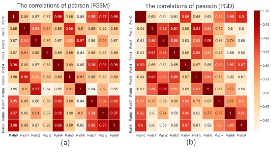
Figure 9. The correlations of pearson corresponding to Top 10 critical detection paths for FGSM and PGD on MNIST.

We can observe that different types anomaly inputs, such as FGSM and PGD, may induce different Pearson correlation coefficients. The Pearson correlation coefficient of PGD is generally smaller than that of FGSM. Correspondingly, combining multiple paths can significantly improve performance for PGD, but not as effective for FGSM, as shown in (a) of Figure 6.

4.8. The Influence of Different Anomaly Samples to the Detection Performance

As presented in Subsection 3.1, for the AD detection task, we use AD data as anomaly samples to select one critical detection path. For the OOD/NS detection task, we use OOD data as anomaly samples to select one critical detection path. To investigate whether this separation is necessary i.e. test the generalization of different critical detection paths in anomaly detection, we conduct experiments to show whether a path selected by using AD samples is suitable in OOD/NS detection, and whether a path selected by using OOD anomaly set is suitable in AD detection. We take the DNN models with in-distribution CIFAR-10 as an example and illustrate the experimental results using the evaluation of AUROC integrated with 21 critical detection paths as shown in Figure 10.

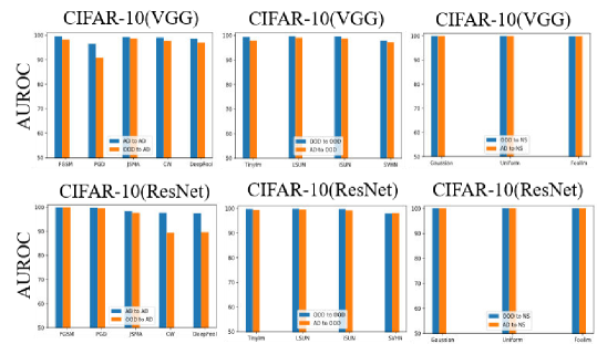
Figure 10. The AUROC corresponding to the paths selected with OOD samples applied to AD detection and the paths selected with AD applied to OOD/NS detection on CIFAR-10.

For the two charts on the left in Fig. 10, a blue bar (AD-to-AD) indicates that the critical detection paths selected by the AD samples are applied to detect AD samples, and an orange bar (OOD-to-AD) indicates that the critical detection paths selected by the OOD samples are applied to detect AD samples. We can see that the performance of OOD-to-AD is slightly less than AD-to-AD for most cases, the difference is large in only a few cases. For the remaining charts, a blue bar (OOD-to-OOD/NS) indicates that the critical detection paths selected by the OOD samples are applied to detect OOD/NS samples and orange bar (AD-to-OOD/NS) indicates that the critical detection paths selected by the AD samples are applied to detect OOD/NS samples. We can see that the performance of AD-to-OOD/NS is basically consistent with OOD-to-OOD/NS for most cases. In summary, the paths selected by different anomaly samples do not have a significant impact on the detection performance, even though the path selected by the specific types of anomaly samples applied to detect the corresponding anomaly sample can get better results.

4.9. Time complexity

In this section, we analyze the time overhead of NPC, EffPath and our approach, regarding path generation. Note that our approach aims to find several critical paths for each class, and we determine whether an input $x$ is anomaly based on the features of these critical paths. NPC and EffPath apply profiling on the entire sample set by generating a path (which may contain multiple neurons per layer) for each input. A final path is then abstracted from all individually generated paths from the inputs. For these two approaches, whether an input is anomaly is determined by comparing its path information and the abstracted path information generated from the training set. Therefore, the time overhead of our approach is mainly the time of extracting one critical path with iterative mutation, and the time overhead of NPC and EffPath mainly depends on the size of a training set. Here, we record the time of $5000$ mutations of our approach and the time of evaluating adversarial samples with $21$ critical paths, as shown in the Table 8. We record the time of extracting the path for one sample and the total time of extracting the paths on the training set for NPC and EffPath, as shown in the Table 9.

From the Table 8, we can observe that both the number of samples and the depth (the number of layers) of the target model affect the time overhead for our approach. Taking the CIFAR-10 and SVHN as an example, we use a 16-layer VGG model with the same structure as target model, while the time overhead on SVHN is significantly higher than that on CIFAR-10 as the number of samples on SVHN is larger than that on CIFAR-10. SVHN has $73,257$ and $26,032$ samples on the training set and test set, while CIFAR-10 has $50,000$ and $10,000$ samples on the training set and test set respectively. When we extract critical path, our approach need train SVDD models and calculate $TPR$. Therefore, the larger the number of samples, the longer the time is consumed. The deeper the target model, the more features are input the SVDD models, and the more time also are consumed to train the SVDD models.

From the Table 9, we can observe that the time overhead also depends on the number of samples and the depth of the target model for NPC and EffPath. Since we need to calculate the path information for each sample separately, the larger number of samples in the training set, the more time will be consumed for the same model. Especially, we can observe that with the increase of the number of model layers, the time overhead increases significantly for different target models. This is mainly because both methods need to calculate the path information layer by layer, and the more layers, the greater amount of computation. In addition, EffPath is slightly more efficient than NPC as EffPath sets a threshold in advance and only selects neurons which have the activation values larger than the threshold as critical neurons to form a critical path, while NPC needs to calculate the relevance of all neurons and then select the critical neurons according to the size on the relevance to form the critical path. Therefore, for EffPath, the number of neurons which require calculation is smaller than NPC.

Table 8. Time complexity of critical operations for ADCP (Seconds).

Model	Dataset	Enumerate $5000$ times	Evaluation	Total
LeNet	MNIST	5740.32	44.01	5514.33
VGG	CIFAR-10	9680.53	70.97	9751.50
ResNet	CIFAR-10	19563.68	132.25	19695.93
VGG	SVHN	26743.37	239.91	26983.28
ResNet	SVHN	30722.56	259.31	30981.87

Table 9. Time complexity of extracting the path for one sample to NPC and EffPath (Seconds).

Model	Dataset	NPC	EffPath	NPC (Training set)	EffPath (Training set)
LeNet	MNIST	0.39	0.34	23400.00	20400.00
VGG	CIFAR-10	9.43	5.72	471500.00	28600.00
ResNet	CIFAR-10	32.25	24.13	1612500.00	1206500.00
VGG	SVHN	9.38	5.81	687150.66	425623.17
ResNet	SVHN	16.06	11.84	1176507.42	867362.88

5. Related Works

In this section we summarize the existing literature related to our work.

5.1. Anomaly Detection

Existing works for anomaly detection either focus on AD detection, e.g.,  (Feinman et al., 2017; Ma et al., 2018b; Cohen et al., 2020; Xu et al., 2018; Vacanti and Van Looveren, 2020; Ma and Liu, 2019; Meng and Chen, 2017), or OOD and NS-1 detection, e.g., (Hendrycks and Gimpel, 2017; Liang et al., 2018; Abdelzad et al., 2019; Hendrycks et al., 2019b; Hsu et al., 2020; Gong et al., 2019), or both (Lee et al., 2018; Zhao et al., 2022; Raghuram et al., 2021; Lust and Condurache, 2022). Notably only one work is capable of detection all types (Zhao et al., 2022) with acceptable performance. All these anomaly detection methods are based on the features of one layer or several layers of the DNN model. For example, Ma et al. (Ma and Liu, 2019) considered the features of each layer of the DNN model, and proposed Network Invariant Checking (NIC) for the detection of AD data. Lee et al. (Lee et al., 2018) calculated the Mahalanobis distance by utilizing the features of each layer of the DNN model for the detection of AD and OOD/NS-I data. Hendrycks et al. (Hendrycks and Gimpel, 2017) and Liang et al. (Liang et al., 2018) analyze the output of DNN models for the detection of OOD/NS-I data. Zhao et al. utilized the outputs of the discriminative layer and the logit layer of a DNN model for detecting three types of anomaly samples (Zhao et al., 2022). We compared our approach with all these methods and the experimental results are shown in Section 4.

The existing work has proved that the features extracted by each layer of a DNN model are different (Dosovitskiy and Brox, 2016). Therefore, it is reasonable to assume that detection accuracy of the existing methods can be further improved as they only rely on a specific layer to detect anomaly samples. For the methods that consider the features of several layers, they essentially obtain a detection result based on the features of each layer, and then integrate the results to obtain a final result. However, during the integration process, anomaly samples are usually used to tune parameters (Lee et al., 2018). This is often unrealistic in real-world applications.

Due to the above defects for the existing anomaly detection methods based on features of layers, in recent years, some works jump out the layer-based paradigm, and look for vulnerabilities in neural networks from the perspective of software testing (Pei et al., 2017; Ma et al., 2018a; Kim et al., 2019; Wang et al., 2019a; Shen et al., 2018; Sun et al., 2018). Among these methods, the methods based on the neuron coverage have got much attention (Pei et al., 2017; Ma et al., 2018a; Kim et al., 2019). Based on the neuron coverage, DeepPath (Wang et al., 2019b) initially proposes the path-driven coverage criteria, which considers the sequentially linked connections of a DNN, and the generated paths represent the information transmission in the entire DNN model. At present, some works have focused on the idea of path-based anomaly detection, and proposed methods to extract the decision logic paths and the adversarial perturbation paths of a DNN model.

5.2. Critical Paths Extraction

Several works have been devoted to interpreting deep neural models by extracting critical paths (Yu et al., 2018; Wang et al., 2018; Qiu et al., 2019; Zhang et al., 2020; Xie et al., 2022; Li et al., 2021). These works can be classified into two categories depending on their application: used for anomaly detection, or used for interpreting a model’s decision procedure.

For the works related to anomaly detection, Wang et al. (Wang et al., 2018) used knowledge distillation (Hinton et al., 2006) to extract critical data routing paths (CDRPs) by learning associated control gates for each layer’s output channel. They use the information of CDRPS to detect adversarial examples. Jiang et al. (Wang et al., 2018) used a similar method to extract critical paths for detecting backdoor attacks. Backdoor attacks are launched by triggers, which are well-designed patterns stuck on images, and aim to mislead DNN models to generate wrong predictions (Gu et al., 2019). Although these two methods have shown good performance in detecting adversarial samples and backdoor attacks, they do not have the merge capability, as a single channel can have different significance values for different images. As such, these methods have weak generalizability (Qiu et al., 2019). To this end, Qiu et al. (Qiu et al., 2019) tried to extract synapse-wise effective paths for each class through network profiling, which contains the neurons and connections that have a positive effect on the prediction results. They use an effective path similarity based method to detect adversarial samples. It calculates the similarity of the effective paths between one test sample and the normal samples. Theoretically, the similarity values of normal samples is higher than that of adversarial samples. However, when the anomaly sample is predicted as a target class with high confidence, its effective path is similar to normal ones, which makes this method invalid (as shown in our evalution in Table 7). Since the method of effective paths only considers the neurons with a positive effect on the prediction results, their effective paths may be incomplete and imprecise. Zhang et al. (Zhang et al., 2020) proposed a method to extract critical paths for each class by using the idea of program slicing, with regard to the effective path, their paths contain neurons and synapses that play a positive and negative contribution in the prediction results.

Regarding critical paths used in interpreting model decision, recently, Xie et al. (Xie et al., 2022) analyzed the relevance of each neuron with the prediction results by using the Layer-wise Relevance Propagation method, and the decision logic paths contain neurons with high relevance (referred to as the NPC method). Li et al. (Li et al., 2021) proposed a gradient-based influence layer-wise propagation method to extract critical attacking paths, and these paths contain neurons with high gradient values.

We have made a detailed discussion regarding the limitations of aforementioned methods in Section 1. In Section 4, we have also compared our approach with two of them (i.e., Effective Path (Qiu et al., 2019) and NPC (Xie et al., 2022)) which have the executable code available to the public.

6. Conclusion and Future Work

We propose a novel approach called Anomaly Detection Based on Critical Paths (ADCP) based on an evolution and mutation mechanism to extract critical detection paths. This approach does not modify the DNN structure and it extracts meaningful path information that can be used to distinguish between normal data and anomaly data. Through the analysis, we also find that we can further enhance performance via an ensemble methodology with multiple critical detection paths. Moreover, our method generalizes to a broad range of anomaly samples, including adversarial inputs (AD), out-of-distribution inputs (OOD), and noise inputs (NS), all with satisfactory performance. Finally, we have conducted extensive experiments to evaluate our approaches, showing that it outperforms state-of-the-art approaches.

One limitation is that this work focus only on image classification. As the application domains of DNN is expanding fast, it is interesting and necessary to explore whether the existing methodology can be adopted to other applications beyond image processing, such as speech recognition, natural language processing, and intrusion detection with network traffic monitoring. Moreover, the key operation of our approach as described in Algorithm 1 may be regarded too expensive in some scenarios which will limit its applicability, especially for large target DNNs and large class sizes. Finally, the method that we used to extract critical path can be further improved as it lacks mathematical proof. In the future, we will explore better and more effective methods for selecting critical path, so as to further enhance the interpretability of our detection results.

*****References

- (1)
- Abdelzad et al. (2019) Vahdat Abdelzad, Krzysztof Czarnecki, Rick Salay, Taylor Denouden, Sachin Vernekar, and Buu Phan. 2019. Detecting Out-of-Distribution Inputs in Deep Neural Networks Using an Early-Layer Output. CoRR abs/1910.10307 (2019). arXiv:1910.10307 http://arxiv.org/abs/1910.10307
- Carlini and Wagner (2017) N. Carlini and D. Wagner. 2017. Towards Evaluating the Robustness of Neural Networks. In Proceedings of 2017 IEEE Symposium on Security and Privacy (IEEE S&P-2017). 39–57.
- Cohen et al. (2020) G. Cohen, G. Sapiro, and R. Giryes. 2020. Detecting Adversarial Samples Using Influence Functions and Nearest Neighbors. In Proceedings of 2020 IEEE/CVF Conference on Computer Vision and Pattern Recognition (CVPR 2020). 14441–14450.
- Deng et al. (2009) J. Deng, W. Dong, R. Socher, L. Li, Kai Li, and Li Fei-Fei. 2009. ImageNet: A large-scale hierarchical image database. In Proceedings of 2009 IEEE Conference on Computer Vision and Pattern Recognition (CVPR 2009). 248–255.
- Dosovitskiy and Brox (2016) Alexey Dosovitskiy and Thomas Brox. 2016. Inverting visual representations with convolutional networks. In Proceedings of the IEEE conference on computer vision and pattern recognition(CVPR2016). 4829–4837.
- Feinman et al. (2017) R. Feinman, R. R. Curtin, S. Shintre, and A. B. Gardner. 2017. Detecting Adversarial Samples from Artifacts. arXiv 1703.00410.
- Floreano and Mattiussi (2008) Dario Floreano and Claudio Mattiussi. 2008. Bio-inspired artificial intelligence: theories, methods, and technologies. MIT press.
- Gong et al. (2019) Dong Gong, Lingqiao Liu, Vuong Le, Budhaditya Saha, Moussa Reda Mansour, Svetha Venkatesh, and Anton van den Hengel. 2019. Memorizing Normality to Detect Anomaly: Memory-augmented Deep Autoencoder for Unsupervised Anomaly Detection. In IEEE International Conference on Computer Vision (ICCV 2019).
- Goodfellow et al. (2015) I. J. Goodfellow, J. Shlens, and C. Szegedy. 2015. Explaining and Harnessing Adversarial Examples. In Proceedings of International Conference on Learning Representations (ICLR 2015).
- Gu et al. (2019) Tianyu Gu, Kang Liu, Brendan Dolan-Gavitt, and Siddharth Garg. 2019. BadNets: Evaluating Backdooring Attacks on Deep Neural Networks. IEEE Access 7 (01 2019), 47230–47244. https://doi.org/10.1109/ACCESS.2019.2909068
- He et al. (2016) Kaiming He, Xiangyu Zhang, Shaoqing Ren, and Jian Sun. 2016. Deep residual learning for image recognition. In Proceedings of the IEEE conference on computer vision and pattern recognition (CVPR 2016). 770–778.
- Hendrycks and Gimpel (2017) D. Hendrycks and K. Gimpel. 2017. A Baseline for Detecting Misclassified and Out-of-Distribution Examples in Neural Networks. In International Conference on Learning Representations (ICLR2017).
- Hendrycks et al. (2019a) Dan Hendrycks, Mantas Mazeika, and Thomas Dietterich. 2019a. Deep Anomaly Detection with Outlier Exposure. In International Conference on Learning Representations (ICLR2019).
- Hendrycks et al. (2019b) D. Hendrycks, M. Mazeika, and T. Dietterich. 2019b. Deep anomaly detection with outlier exposure. In International Conference on Learning Representations (ICLR2019).
- Hinton et al. (2006) Geoffrey E Hinton, Simon Osindero, and Yee-Whye Teh. 2006. A fast learning algorithm for deep belief nets. Neural computation 18, 7 (2006), 1527–1554.
- Ho (1998) Tin Kam Ho. 1998. The random subspace method for constructing decision forests. IEEE transactions on pattern analysis and machine intelligence 20, 8 (1998), 832–844.
- Hsu et al. (2020) Y.-C. Hsu, Y. Shen, H. Jin, and Z. Kira. 2020. Generalized ODIN: Detecting Out-of-Distribution Image Without Learning From Out-of-Distribution Data. In 2020 IEEE/CVF Conference on Computer Vision and Pattern Recognition (CVPR2020). 10948–10957.
- Kim et al. (2019) Jinhan Kim, Robert Feldt, and Shin Yoo. 2019. Guiding deep learning system testing using surprise adequacy. In 2019 IEEE/ACM 41st International Conference on Software Engineering (ICSE). IEEE, 1039–1049.
- Krizhevsky et al. (2012) Alex Krizhevsky, Ilya Sutskever, and Geoffrey E Hinton. 2012. Imagenet classification with deep convolutional neural networks. Advances in neural information processing systems (NIPS 2012) 25 (2012), 1097–1105.
- Lake et al. (2015) B. M. Lake, R. Salakhutdinov, and J. B. Tenenbaum. 2015. Human-level concept learning through probabilistic program induction. Science 350, 6266 (2015), 1332–1338.
- Lee et al. (2018) K. Lee, K. Lee, H. Lee, and J. Shin. 2018. A Simple Unified Framework for Detecting Out-of-Distribution Samples and Adversarial Attacks. In Proceedings of the 32nd International Conference on Neural Information Processing SystemsDecember (NeurIPS 2018). 7167–7177.
- Li et al. (2021) Tianlin Li, Aishan Liu, Xianglong Liu, Yitao Xu, Chongzhi Zhang, and Xiaofei Xie. 2021. Understanding adversarial robustness via critical attacking route. Information Sciences 547 (2021), 568–578.
- Liang et al. (2018) S. Liang, Y. Li, and R. Srikant. 2018. Enhancing The Reliability of Out-of-distribution Image Detection in Neural Networks. In International Conference on Learning Representations (ICLR2018).
- Lust and Condurache (2020) Julia Lust and Alexandru Paul Condurache. 2020. A Survey on Assessing the Generalization Envelope of Deep Neural Networks: Predictive Uncertainty, Out-of-distribution and Adversarial Samples. arXiv preprint arXiv:2008.09381 (2020).
- Lust and Condurache (2022) Julia Lust and Alexandru P Condurache. 2022. Efficient detection of adversarial, out-of-distribution and other misclassified samples. Neurocomputing 470 (2022), 335–343.
- Ma et al. (2018a) Lei Ma, Felix Juefei-Xu, Fuyuan Zhang, Jiyuan Sun, Minhui Xue, Bo Li, Chunyang Chen, Ting Su, Li Li, Yang Liu, et al. 2018a. Deepgauge: Multi-granularity testing criteria for deep learning systems. In Proceedings of the 33rd ACM/IEEE International Conference on Automated Software Engineering. 120–131.
- Ma et al. (2018c) Lei Ma, Fuyuan Zhang, Jiyuan Sun, Minhui Xue, Bo Li, Felix Juefei-Xu, Chao Xie, Li Li, Yang Liu, Jianjun Zhao, et al. 2018c. Deepmutation: Mutation testing of deep learning systems. In 2018 IEEE 29th International Symposium on Software Reliability Engineering (ISSRE). IEEE, 100–111.
- Ma and Liu (2019) Shiqing Ma and Yingqi Liu. 2019. Nic: Detecting adversarial samples with neural network invariant checking. In Proceedings of the 26th network and distributed system security symposium (NDSS 2019).
- Ma et al. (2018b) X. Ma, B. Li, Y. Wang, M. S. Erfani, N. R. S. Wijewickrema, E. M. Houle, G. Schoenebeck, D. Song, and J. Bailey. 2018b. Characterizing Adversarial Subspaces Using Local Intrinsic Dimensionality. In Proceedings of International Conference on Learning Representations (ICLR 2018).
- Meng and Chen (2017) Dongyu Meng and Hao Chen. 2017. Magnet: a two-pronged defense against adversarial examples. In Proceedings of the 2017 ACM SIGSAC conference on computer and communications security (CCS 2017). 135–147.
- Moosavi-Dezfooli et al. (2016) Seyed-Mohsen Moosavi-Dezfooli, Alhussein Fawzi, and Pascal Frossard. 2016. Deepfool: a simple and accurate method to fool deep neural networks. In Proceedings of the IEEE conference on computer vision and pattern recognition. 2574–2582.
- Netzer et al. (2011) Y. Netzer, T. Wang, A. Coates, A. Bissacco, B. Wu, and A. Ng. 2011. Reading Digits in Natural Images with Unsupervised Feature Learning. In Proceedings of NIPS Workshop on Deep Learning and Unsupervised Feature Learning (NIPS 2011 Workshop).
- Nguyen et al. (2015) A. Nguyen, J. Yosinski, and J. Clune. 2015. Deep Neural Networks are Easily Fooled: High Confidence Predictions for Unrecognizable Images. In Proceedings of 2015 IEEE Conference on Computer Vision and Pattern Recognition (CVPR 2015). 427–436.
- Papernot et al. (2018) Nicolas Papernot, Fartash Faghri, Nicholas Carlini, Ian Goodfellow, Reuben Feinman, Alexey Kurakin, Cihang Xie, et al. 2018. Technical Report on the CleverHans v2.1.0 Adversarial Examples Library. arXiv preprint arXiv:1610.00768 (2018).
- Papernot et al. (2016) N. Papernot, P. D. McDaniel, S. Jha, M. Fredrikson, Z. B. Celik, and A. Swami. 2016. The Limitations of Deep Learning in Adversarial Settings. In Proceedings of 2016 IEEE European Symposium on Security and Privacy (EuroS&P-2016). 372–387.
- Pei et al. (2017) Kexin Pei, Yinzhi Cao, Junfeng Yang, and Suman Jana. 2017. Deepxplore: Automated whitebox testing of deep learning systems. In proceedings of the 26th Symposium on Operating Systems Principles. 1–18.
- Qiu et al. (2019) Yuxian Qiu, Jingwen Leng, Cong Guo, Quan Chen, Chao Li, Minyi Guo, and Yuhao Zhu. 2019. Adversarial defense through network profiling based path extraction. In the IEEE/CVF Conference on Computer Vision and Pattern Recognition(CVPR2019). 4777–4786.
- Raghuram et al. (2021) Jayaram Raghuram, Varun Chandrasekaran, Somesh Jha, and Suman Banerjee. 2021. A general framework for detecting anomalous inputs to DNN classifiers. In International Conference on Machine Learning. PMLR, 8764–8775.
- Ren et al. (2019) Jie Ren, Peter J Liu, Emily Fertig, Jasper Snoek, Ryan Poplin, Mark Depristo, Joshua Dillon, and Balaji Lakshminarayanan. 2019. Likelihood ratios for out-of-distribution detection. Advances in Neural Information Processing Systems (NiPS2019) 32 (2019).
- Ruff et al. (2018) Lukas Ruff, Robert Vandermeulen, Nico Goernitz, Lucas Deecke, Shoaib Ahmed Siddiqui, Alexander Binder, Emmanuel Müller, and Marius Kloft. 2018. Deep One-Class Classification. In Proceedings of the 35th International Conference on Machine Learning (Proceedings of Machine Learning Research, Vol. 80), Jennifer Dy and Andreas Krause (Eds.). PMLR, Stockholmsmässan, Stockholm Sweden, 4393–4402. http://proceedings.mlr.press/v80/ruff18a.html
- Ruff et al. (2020) Lukas Ruff, Robert A. Vandermeulen, Nico Görnitz, Alexander Binder, Emmanuel Müller, Klaus-Robert Müller, and Marius Kloft. 2020. Deep Semi-Supervised Anomaly Detection. In International Conference on Learning Representations. https://openreview.net/forum?id=HkgH0TEYwH
- Sastry and Oore (2020) Chandramouli Shama Sastry and Sageev Oore. 2020. Detecting out-of-distribution examples with gram matrices. In International Conference on Machine Learning(ICML2020). PMLR, 8491–8501.
- Schölkopf et al. (2001) B. Schölkopf, J. C. Platt, J. C. Shawe-Taylor, A. J. Smola, and R. C. Williamson. 2001. Estimating the Support of a High-Dimensional Distribution. Neural Computation 13, 7 (2001), 1443–1471.
- Shen et al. (2018) Weijun Shen, Jun Wan, and Zhenyu Chen. 2018. MuNN: Mutation Analysis of Neural Networks. In 2018 IEEE International Conference on Software Quality, Reliability and Security Companion (QRS-C). 108–115. https://doi.org/10.1109/QRS-C.2018.00032
- Sun et al. (2018) Youcheng Sun, Min Wu, Wenjie Ruan, Xiaowei Huang, Marta Kwiatkowska, and Daniel Kroening. 2018. Concolic Testing for Deep Neural Networks. In 2018 33rd IEEE/ACM International Conference on Automated Software Engineering (ASE). 109–119. https://doi.org/10.1145/3238147.3238172
- Tax (2001) D. Tax. 2001. One-class classification: Concept-learning in the absence of counter-examples. Ph. D. Dissertation. Delft University of Technology.
- Tax and Duin (1999) D. M. J. Tax and R. P. W. Duin. 1999. Support vector domain description. Pattern Recognit. Letters. 20, 11-13 (1999), 1191–1199.
- Vacanti and Van Looveren (2020) Giovanni Vacanti and Arnaud Van Looveren. 2020. Adversarial detection and correction by matching prediction distributions. arXiv preprint arXiv:2002.09364 (2020).
- Vapnik (2000) V. Vapnik. 2000. The Nature of Statistical Learning Theory. Springer.
- Wang et al. (2019b) Dong Wang, Ziyuan Wang, Chunrong Fang, Yanshan Chen, and Zhenyu Chen. 2019b. DeepPath: Path-driven testing criteria for deep neural networks. In 2019 IEEE International Conference On Artificial Intelligence Testing (AITest). IEEE, 119–120.
- Wang et al. (2019a) Jingyi Wang, Guoliang Dong, Jun Sun, Xinyu Wang, and Peixin Zhang. 2019a. Adversarial sample detection for deep neural network through model mutation testing. In 2019 IEEE/ACM 41st International Conference on Software Engineering (ICSE). IEEE, 1245–1256.
- Wang et al. (2018) Yulong Wang, Hang Su, Bo Zhang, and Xiaolin Hu. 2018. Interpret neural networks by identifying critical data routing paths. In the IEEE conference on computer vision and pattern recognition(CVPR2018). 8906–8914.
- Xiao et al. (2017) H. Xiao, K. Rasul, and R. Vollgraf. 2017. Fashion-MNIST: A Novel Image Dataset for Benchmarking Machine Learning Algorithms. arXiv 1708.07747.
- Xie et al. (2022) Xiaofei Xie, Tianlin Li, Jian Wang, Lei Ma, Qing Guo, Felix Juefei-Xu, and Yang Liu. 2022. NPC: N euron P ath C overage via Characterizing Decision Logic of Deep Neural Networks. ACM Transactions on Software Engineering and Methodology (TOSEM) 31, 3 (2022), 1–27.
- Xu et al. (2015) P. Xu, K. A. Ehinger, Y. Zhang, A. Finkelstein, S. R. Kulkarni, and J. Xiao. 2015. TurkerGaze: Crowdsourcing Saliency with Webcam based Eye Tracking. arXiv 1504.06755.
- Xu et al. (2018) W. Xu, D. Evans, and Y. Qi. 2018. Feature Squeezing: Detecting Adversarial Examples in Deep Neural Networks. In Proceedings of The Network and Distributed System Security (NDSS 2018).
- Yu et al. (2018) Fuxun Yu, Zhuwei Qin, and Xiang Chen. 2018. Distilling critical paths in convolutional neural networks. arXiv preprint arXiv:1811.02643 (2018).
- Yu et al. (2015) F. Yu, Y. Zhang, S. Song, A. Seff, and J. Xiao. 2015. LSUN: Construction of a Large-scale Image Dataset using Deep Learning with Humans in the Loop. arXiv 1506.03365.
- Zhang et al. (2020) Ziqi Zhang, Yuanchun Li, Yao Guo, Xiangqun Chen, and Yunxin Liu. 2020. Dynamic slicing for deep neural networks. In the 28th ACM Joint Meeting on European Software Engineering Conference and Symposium on the Foundations of Software Engineering(ESEC/FSE-2020). 838–850.
- Zhao et al. (2022) Fangzhen Zhao, Chenyi Zhang, Naipeng Dong, Zefeng You, and Zhenxin Wu. 2022. A Uniform Framework for Anomaly Detection in Deep Neural Networks. Neural Processing Letters (2022), 1–22.