minitoc(hints)W0018 minitoc(hints)W0028 minitoc(hints)W0030 blindtext IJOC-0001-2024.00

Yongchun Li

Strong Formulations and Algorithms for Regularized A-optimal Design

Strong Formulations and Algorithms for Regularized A-optimal Design

Yongchun Li Department of Industrial and Systems Engineering, University of Tennessee, Knoxville, ycli@utk.edu

We study the Regularized A-optimal Design (RAOD) problem, which selects a subset of $k$ experiments to minimize the inverse of the Fisher information matrix, regularized with a scaled identity matrix. RAOD has broad applications in Bayesian experimental design, sensor placement, and cold-start recommendation. We prove its NP-hardness via a reduction from the independent set problem. By leveraging convex envelope techniques, we propose a new convex integer programming formulation for RAOD, whose continuous relaxation dominates those of existing formulations. More importantly, we demonstrate that our continuous relaxation achieves bounded optimality gaps for all $k$, whereas previous relaxations may suffer from unbounded gaps. This new formulation enables the development of an exact cutting-plane algorithm with superior efficiency, especially in high-dimensional and small-$k$ scenarios. We also investigate scalable forward and backward greedy algorithms for solving RAOD, each with provable performance guarantees for different $k$ ranges. Finally, our numerical results on synthetic and real data demonstrate the efficacy of the proposed exact and approximation algorithms. We further showcase the practical effectiveness of RAOD by applying it to a real-world user cold-start recommendation problem.

Regularized A-optimality, Mixed-integer nonlinear optimization, Convex relaxations, Cutting-plane algorithm, Forward and backward greedy algorithms, User cold-start recommendation

1 Introduction

The A-optimal Design (AOD) problem arises in statistical design for situations where, due to budget limitations, one can observe the outcomes for a small subset of experiments to optimize the parameter estimates. Specifically, AOD aims to minimize the trace of the inverse of the Fisher information matrix, resulting in minimizing the average variance of the parameter estimates. AOD has found broad applications in fields such as engineering (Ilzarbe et al. 2008, Mason et al. 2003), biology (Quinn and Keough 2002), and chemistry (Higgs et al. 1997, Leardi 2009), when dealing with large-scale and costly experiments. Linear regression models are one of the most widely used and studied models in this area (see, Jobson 2012, Nikolov et al. 2022, Winer et al. 1971). This paper focuses on the Regularized AOD (RAOD) problem in the context of linear regression models, which adds a scaled identity matrix to the Fisher information matrix, as shown below. This addition typically helps prevent over-fitting (Tantipongpipat 2020), improves numerical stability when the information matrix is rank-deficient (Dereziński and Warmuth 2017), and encodes prior information (Bian et al. 2017).

$$z_{k}:=\min_{S\subseteq[n]}\bigg{\{}\operatorname{tr}\bigg{(}\bigg{(}\sum_{i\in S}\bm{a}_{i}\bm{a}_{i}^{\top}+\lambda\bm{I}_{d}\bigg{)}^{-1}\bigg{)}:|S|=k\bigg{\}},$$ (RAOD)

where $\{\bm{a}_{i}\}_{i\in[n]}\in{\mathbb{R}}^{d}$ represents a collection of $n$ experiments parameterized by $d$-dimensional vectors with $d\leq n$, $k\leq n$ denotes the number of chosen experiments, $\lambda>0$ is a constant, $\bm{I}_{d}$ is a $d\times d$ identity matrix, and for a subset $S\subseteq[n]$, let $|S|$ denote its cardinality. Note that the selection size $k$ can be smaller or larger than the dimension $d$, depending on the specific problem setup.

The following outlines the two most relevant variants and an equivalent problem of RAOD, which will be used throughout to show the scope and limitations of existing research, facilitate our analysis, and highlight the general applicability of some of our results.

1. AOD. As previously mentioned, $\lambda$ is fixed at zero in AOD. It is noted that the condition $k\geq d$ must hold for AOD to ensure that the objective matrix is invertible;

2. Bayesian AOD. Since specific information is usually available prior to the experimental selection process, Bayesian AOD, which leverages prior knowledge, can play an important role in improving design efficiency (see the excellent survey by Chaloner and Verdinelli 1995, Rainforth et al. 2024). Mathematically, it generalizes the scaled identity matrix in RAOD to an arbitrary positive definite matrix representing prior information. Bayesian AOD is also referred to as the A-Fusion problem in Hendrych et al. (2023). When the prior is an isotropic Gaussian, Bayesian AOD reduces to RAOD as a special case (see, e.g., Bian et al. 2017, Chamon and Ribeiro 2017a); and

3. A-optimal Maximum Entropy Sampling Problem (AMESP). As introduced in Li and Xie (2024), AMESP focuses on selecting the most informative principal submatrix from a given covariance matrix by minimizing the trace of its inverse. We are the first to demonstrate that RAOD and AMESP are equivalent, with an additive additional constant of $(d-k)/\lambda$, when the covariance matrix in AMESP is positive definite.

Although RAOD is a special case of Bayesian AOD, it remains broadly applicable. One key motivation comes from the user cold-start problem in recommendation systems. The problem arises when a new user joins a recommendation platform and has not rated any item, making recommendations challenging due to the lack of historical data (Lika et al. 2014).

Traditional methods, such as content-based filtering and collaborative filtering, exploit relationships and similarities between users to make recommendations (Bobadilla et al. 2012, Volkovs et al. 2017). Alternatively, experimental design approaches, including sequential strategies, tackle the problem at its root by explicitly asking new users to rate selected items upon joining a recommendation platform (see, e.g., Anava et al. 2015, Elahi et al. 2016, Gope and Jain 2017). These items are selected carefully to capture new users’ preferences. However, users are often reluctant to rate many items due to cognitive costs. If users rate too few items, the Fisher information matrix becomes rank-deficient, leading to ill-posed matrix inverse and determinant problems in experimental design. To mitigate this, regularized experimental design has emerged as a practical approach by adding a scaled identity matrix, as shown in prior research by Barz et al. (2015), Anava et al. (2015), Rubens et al. (2009). In particular, Chamon and Ribeiro (2017a) applied the RAOD approach and demonstrated its effectiveness in selecting movies for new users to rate.

1.1 Related Work

In this subsection, we review the relevant literature on RAOD and its variants, with a focus on their exact algorithms, convex relaxations, and approximation algorithms.

Bayesian D-optimal Design (Bayesian DOD) & Bayesian AOD. In experimental designs, the $D$- and A-optimality criteria are widely used for selecting experiments to achieve precise parameter estimation. A-optimality minimizes the estimation variance directly, while D-optimality seeks to reduce the volume of the confidence ellipsoid of the parameter estimates by maximizing the determinant of the Fisher information matrix. Notably, given that the determinant is a multiplicative operator, Bayesian DOD is equivalent to regularized DOD (Li et al. 2024); however, this equivalence does not hold between Bayesian AOD and RAOD.

A-optimality is known to be computationally more expensive than D-optimality due to its need to compute the inverse matrix (Ahipaşaoglu 2021). As a result, algorithms and software for Bayesian DOD are more developed than Bayesian AOD (see Jones et al. 2021). Unfortunately, these techniques cannot be directly applied to Bayesian AOD. Nevertheless, Bayesian AOD often outperforms Bayesian DOD, with improved variance and bias properties (see, e.g., Jones et al. 2021, Stallrich et al. 2023). Our numerical study on cold-start recommendation further shows the superior performance of RAOD compared to regularized DOD. In addition, DOD, AOD, and Bayesian DOD have been proven to be NP-hard, see Welch (1982), Nikolov et al. (2022), Li et al. (2024), respectively. In contrast, the complexity of Bayesian AOD remains an open question, though Hendrych et al. (2023) conjectured that it was NP-hard. The limited literature on Bayesian AOD motivates us to develop efficient algorithms for its special case, RAOD. While this paper does not address the general Bayesian AOD problem, we demonstrate its NP-hardness for the first time.

Exact Algorithms. Experimental design problems can be formulated as mixed-integer nonlinear programs (MINLPs) by introducing binary variables to represent subset selection. In view of this, advancing exact solution methods for these MINLPs has been a longstanding research focus. Given the complexity of the A-optimality function, RAOD and its variants naturally reduce to mixed-integer semidefinite programs (MISDPs) (Duarte 2023). To solve these MISDPs, the branch-and-bound (B&B) method has been extensively studied in the literature (see, e.g., Ahipaşaoglu 2021, Hendrych et al. 2023, Liang and Yang 2024). These works leveraged the standard continuous relaxation of RAOD to provide a lower bound, referred to as RAOD-RI throughout this paper, which is also reviewed in detail below.

An alternative approach formulates RAOD and its variants as mixed-integer second-order cone programs (MISOCPs). It is worth noting that unlike MISDP, modern optimization solvers such as Gurobi and CPLEX are well-suited for solving MISOCP. Sagnol (2011) pioneered this direction by applying Elfving’s Theorem to demonstrate the second-order representability of the continuous relaxation of AOD, and it is actually a consequence of Gauss–Markov Theorem. Duarte and Wong (2015) later extended the result to the Bayesian version. Building on these, a seminar work by Sagnol and Harman (2015) developed exact MISOCP reformulations of AOD and Bayesian AOD.

Convex Relaxation. A natural way to get rid of the integer challenge is relaxing the binary variables in the exact MISDP reformulation of RAOD to be continuous, which leads to the convex relaxation RAOD-RI. Much of the literature on the relaxation has focused on developing efficient convex optimization algorithms, see Ahipaşaoglu (2015), Liang and Yang (2024), and many references therein. However, despite these computational advancements, we demonstrate that RAOD-RI may perform poorly when $k$ is within the range of $[d-1]$. This limitation motivates us to develop stronger relaxations, which are important for improving the efficiency of exact algorithms.

Approximation Algorithms. Avron and Boutsidis (2013) studied the classic AOD problem and proposed volume-sampling-based algorithms that achieved an approximation ratio of $(n-d+1)/(k-d+1)$ for $k\in[d,n]$. The result was later extended to RAOD by Dereziński and Warmuth (2017) in the same regime of $k$, who developed a faster ${\mathcal{O}}(nd^{2})$-time sampling algorithm.

Another approach to developing sampling algorithms is based on convex relaxations. These algorithms start from solving a convex relaxation and then, based on the continuous solution, design randomized sampling strategies to obtain a discrete solution with approximation guarantees, see Nikolov et al. 2022, Wang et al. 2017 for the classic AOD problem, Tantipongpipat (2020), Li and Xie (2024) for RAOD, and Allen-Zhu et al. (2017), Derezinski et al. (2020) for Bayesian AOD, respectively. However, these convex relaxation-based sampling algorithms of RAOD often scale poorly with the number of experiments $n$ (see, e.g., the fourth and fifth rows of Table 2). It is important to note that when applying the approximation algorithms developed for AMESP by Li and Xie (2024) to RAOD, an additional constant $(d-k)/\lambda$ must be added, as shown in Proposition 2.1. Hence, their approximation ratios remain valid when $k\leq d$ after adding a nonnegative constant, since for any $c_{1}\geq c_{2}$, it is easy to verify that $\frac{c_{1}+(d-k)/\lambda}{c_{2}+(d-k)/\lambda}\leq\frac{c_{1}}{c_{2}}$. However, these ratios do not hold for $k\in[d+1,n]$, where $(d-k)/\lambda$ becomes negative.

Natural combinatorial algorithms, such as the greedy and local search algorithms, have been widely used in experimental design (see, e.g., Krause et al. 2008, Madan et al. 2019). The forward greedy algorithm has also been extended to Bayesian criteria in Bian et al. (2017), Chamon and Ribeiro (2017b). However, A-optimality is not a supermodular function (Chamon and Ribeiro 2017a), which means that the typical approximation ratio for forward greedy (i.e., $(1-1/e)$) cannot apply. Instead, these greedy methods often achieve data-dependent guarantees, where the worst-case performance can vary significantly with the experimental setup. By data-independence, we mean a theoretical guarantee that does not rely on the experiments $\{\bm{a}_{i}\}_{i\in[n]}$ or $\lambda$ but may depend on the parameters $n,d$, and $k$. We are unaware of any prior work on developing a backward greedy search method in the literature of RAOD. This gap is addressed in our paper. Notably, Li and Xie (2024) proposed a local search algorithm for AMESP with strong empirical performance, but its theoretical guarantee is data-independent. The performance guarantees and complexities of the approximation algorithms reviewed for RAOD are summarized in Table 2.

1.2 Summary of the Organization and Contributions

Below we list the major contributions and an outline of the remaining paper.

1. Complexity analysis. In Section 2, we prove the NP-hardness of RAOD by establishing its equivalence to AMESP and reducing the independent set decision problem to AMESP;

2. Optimality gaps of convex relaxations. Section 3 presents existing (mixed-)integer convex formulations of RAOD and analyzes the optimality gaps of their convex relaxations, as summarized in Table 1. Notably, we show that the conventional relaxation RAOD-RI can have unbounded gaps for $k\in[d-1]$, while the relaxation AMESP-R of AMESP may perform worse than the trivial zero lower bound for $k\in[d+1,n]$. Finally, in Subsection 3.3, we revisit the formulation MISOCP from an optimization perspective and prove that its continuous relaxation coincides with RAOD-RI;

3. New formulations. Motivated by the weaknesses of existing formulations, we propose a novel convex integer programming formulation for RAOD in Section 4, whose continuous relaxation RAOD-RII is tighter than those presented in Section 3. More importantly, RAOD-RII achieves bounded optimality gaps for all $k\in[n]$, which addresses a key drawback of RAOD-RI and AMESP-R. Building on our new formulation, we develop an exact cutting-plane algorithm to solve RAOD to optimality;

4. Greedy algorithms. In Section 5, we first establish a data-independent approximation ratio for the forward greedy algorithm when $k\in[d-1]$. To complement this, we propose a backward greedy algorithm for RAOD and derive its data-independent performance guarantee for $k\in[d,n]$. These results, summarized in Table 2, present a comprehensive analysis of our greedy algorithms across different ranges of $k$; and

5. Numerical study. Finally, in Section 6, our numerical study on synthetic and real data demonstrates the effectiveness of our exact algorithm and the scalability and high-quality outputs of our approximation algorithms. In particular, when applied to the user cold-start problem in movie recommendation systems, RAOD effectively identifies movie subsets that lead to more reliable recommendations for new users in most instances, outperforming its D-optimality counterpart.

Table 1: Summary of convex relaxations for RAOD

Convex relaxation	Optimality gap (i.e., ${z}_{k}$/relaxation value)	Value of $k$
RAOD-RI	Can be arbitrarily large	$k\in[d-1]$
	$\min\left\{d,n-d+1\right\}$	$k=d$
	$\frac{n-d+1}{k-d+1}$	$k\in[d+1,n]$
AMESP-R	$\min\left\{\frac{d-1}{d-k},n-k+1\right\}$	$k\in[d-1]$
	$\min\left\{d,n-d+1\right\}$	$k=d$
	Can be negative	$k\in[d+1,n]$
RAOD-RII	$\min\left\{\frac{d-1}{d-k},n-k+1\right\}$	$k\in[d-1]$
	$\min\left\{d,n-d+1\right\}$	$k=d$
	$\frac{n-d+1}{k-d+1}$	$k\in[d+1,n]$

Table 2: Summary of approximation algorithms for RAOD

Approximation algorithm	Time complexity	Approximation ratio
Sampling (Dereziński and Warmuth 2017)	${\mathcal{O}}((n^{2}+d^{2})d)$	$\frac{n-d+1}{k-d+1}$ if $k\in[d,n]$
Fast sampling (Dereziński and Warmuth 2017)	${\mathcal{O}}((n+d)d^{2})$	$\frac{n-d+1}{k-d+1}$ if $k\in[d,n]$
Forward greedy (Chamon and Ribeiro 2017b)	${\mathcal{O}}(knd^{2})$	$-$i
Sampling (Tantipongpipat 2020)	${\mathcal{O}}(n^{4}dk^{2}\log(dk))$	$-$
Sampling (Li and Xie 2024)	${\mathcal{O}}(n^{4}dk^{2}\log(dk))$	$\min\{k,n-k+1\}$ if $k\in[d]$
Local search (Li and Xie 2024)	${\mathcal{O}}(k(n-k)d^{5})$	$-$
Forward greedy Algorithm 2	${\mathcal{O}}(knd^{2})$	$\frac{d-1}{d-k}$ if $k\in[d-1]$
Backward greedy Algorithm 3	${\mathcal{O}}((n-k)nd^{2})$	$\frac{n-d+1}{k-d+1}$ if $k\in[d,n]$

• “$-$”: The approximation ratio depends on data $\{\bm{a}_{i}\}_{i\in[n]}$ and the constant $\lambda$

Notations. We let ${\mathcal{S}}_{+}^{n},{\mathcal{S}}_{++}^{n}$ denote the set of all the $n\times n$ symmetric positive semidefinite and positive definite matrices, respectively. We let ${\mathbb{R}}^{n}$, $\mathbb{R}_{+}^{n}$, and $\mathbb{R}_{++}^{n}$ denote the set of all the $n$-dimensional vectors, nonnegative vectors, and positive vectors, respectively. We use bold lower-case letters (e.g., $\bm{x}$) and bold upper-case letters (e.g., $\bm{X}$) to denote vectors and matrices, respectively, and use corresponding non-bold letters (e.g., $x_{i}$) to denote their components. Given two positive integers $s\leq n$, we let $[n]=\{1,2,\cdots,n\}$, and let $[s,n]=\{s,s+1,\cdots,n\}$. We let $\bm{I}_{n}$ be the $n\times n$ identity matrix. For a vector $\bm{x}\in{\mathbb{R}}^{n}$, let $\operatorname{Diag}(\bm{x})$ denote a diagonal matrix with diagonal entries being $\bm{x}$ and let $\|\bm{x}\|_{2}$ denote its two norm. If $\bm{x}\in{\mathbb{R}}_{+}^{n}$ is nonnegative, we define $\sqrt{\bm{x}}$ as the vector where each entry is the square root of the corresponding element in $\bm{x}$. For a matrix $\bm{X}\in{\mathbb{R}}^{d\times n}$, we let $\|\bm{X}\|_{F}$ denote its Frobenius norm, let $\bm{X}_{i}\in{\mathbb{R}}^{d}$ denote its $i$-th column vector for each $i\in[n]$, and for a subset $S\subseteq[n]$, let $\bm{X}_{S}$ denote the submatrix consisting of the columns of $\bm{X}$ indexed by $S$. For a symmetric matrix $\bm{X}\in{\mathcal{S}}^{n}_{+}$, let $\operatorname{tr}(\bm{X})$ denote its trace, and for a subset $S\subseteq[n]$, we let $\bm{X}_{S,S}$ denote a principal submatrix of $\bm{X}$ indexed by $S$.

2 Complexity Analysis

We begin by showing the equivalence between RAOD and AMESP with an additional constant of ${(d-k)}/{\lambda}$. Proposition 2.1 extends Li et al. (2024, Theorems 1 and 2), where they demonstrated the equivalence between Bayesian DOD and MESP. Our Proposition 2.1 further connects experimental design problems with maximum entropy-based optimization.

For brevity, we define the objective function of RAOD as

$$f(S):=\operatorname{tr}\bigg{(}\bigg{(}\sum_{i\in S}\bm{a}_{i}\bm{a}_{i}^{\top}+\lambda\bm{I}_{d}\bigg{)}^{-1}\bigg{)}$$

for any subset $S\subseteq[n]$ throughout.

Proposition 2.1

RAOD can be converted into the following:

$$z_{k}=\min_{S\subseteq[n]}\left\{\operatorname{tr}\left(\left(\bm{C}_{S,S}\right)^{-1}\right)+\frac{d-k}{\lambda}:|S|=k\right\},$$ (AMESP)

where $\bm{C}\in{\mathcal{S}}_{+}^{n}:=\bm{A}^{\top}\bm{A}+\lambda\bm{I}_{n}$, and $\bm{A}\in{\mathbb{R}}^{d\times n}$ is a matrix whose columns are vectors $\{\bm{a}_{i}\}_{i\in[n]}$.

Proof 2.2

Proof. See Appendix 8.1. $\square$

It is well known that the independent set decision problem is NP-hard (Cormen et al. 2022, Chapter 34). Next, we prove that the independent set decision problem can be reduced to AMESP, which, combined with Proposition 2.1, establishes the NP-hardness of RAOD.

Definition 2.3 (Independent sets and the independent set decision problem)

In an undirected graph $G$, an independent set $S$ is a set of vertices such that no two vertices in $S$ are adjacent. Given an integer $k$, the independent set decision problem is to determine if the graph $G$ contains an independent set of size $k$.

Let us introduce a known inequality based on the comparison between the harmonic mean and arithmetic mean, which is a key technical result used throughout the paper.

Lemma 2.4 (Sedrakyan and Sedrakyan 2018)

Suppose $\bm{\sigma}\in{\mathbb{R}}_{++}^{n}$. Then, the following holds

$$\sum_{i\in[n]}\frac{1}{\sigma_{i}}\geq\frac{n^{2}}{\sum_{i\in[n]}\sigma_{i}},$$

which becomes an equality if and only if all entries of $\bm{\sigma}$ are equal.

Theorem 2.5 (NP-hardness)

RAOD is NP-hard.

Proof 2.6

Proof. See Appendix 8.2. $\square$

Theorem 2.5 confirms the following conjecture from Hendrych et al. (2023) regarding Bayesian AOD. Since RAOD is a special case of Bayesian AOD, the conjecture is clearly true.

Conjecture 2.7 (Hendrych et al. 2023)

The Bayesian AOD problem is NP-hard.

3 Optimality Gaps of Convex Relaxations

This section presents two widely-used (mixed-)integer convex formulations of RAOD and derives the optimality gaps for their continuous relaxations. Leveraging Proposition 2.1, we further analyze the quality of a convex relaxation for AMESP.

3.1 The Conventional Convex Integer Programming Formulation and its Convex Relaxation

By introducing a binary characterization of the subset $S\subseteq[n]$, where $x_{i}=1$ if $i\in S$ and $x_{i}=0$ otherwise, we can readily obtain a convex integer nonlinear formulation of RAOD

$$z_{k}=\min_{\bm{x}\in\{0,1\}^{n}}\bigg{\{}\operatorname{tr}\bigg{(}\bigg{(}\sum_{i\in[n]}x_{i}\bm{a}_{i}\bm{a}_{i}^{\top}+\lambda\bm{I}_{d}\bigg{)}^{-1}\bigg{)}:\sum_{i\in[n]}x_{i}=k\bigg{\}},$$ (1)

and its continuous relaxation provides a practical lower bound (Tantipongpipat 2020):

$$z_{k}\geq{\nu}_{k}^{\text{C}}:=\min_{\bm{x}\in[0,1]^{n}}\bigg{\{}\operatorname{tr}\bigg{(}\bigg{(}\sum_{i\in[n]}x_{i}\bm{a}_{i}\bm{a}_{i}^{\top}+\lambda\bm{I}_{d}\bigg{)}^{-1}\bigg{)}:\sum_{i\in[n]}x_{i}=k\bigg{\}}.$$ (RAOD-RI)

It is evident that ${\nu}_{k}^{\text{C}}$ is always positive.

The problem (1) can be recast as a MISDP by nature. The conventional relaxation RAOD-RI has been widely incorporated into the B&B algorithms for solving (1) to optimality (e.g., Hendrych et al. 2023). For B&B algorithms, the quality of the relaxation bound used is crucial for pruning the search space. We are thus motivated to explore the quality of RAOD-RI. Before that, let us explore the properties of the objective function $f(S)$ in RAOD. First, the function $f(S)$ decreases monotonically with respect to $S$, that is, $f(S\setminus\{i\})\geq f(S)$ for any $i\in S$. We also remark that

Remark 3.1

The optimal value $z_{k}$ decreases as the selection size $k$ increases. $\diamond$

Lemma 3.2 establishes an upper bound for the smallest value of $f(S\setminus\{i\})$ over $i\in S$. Our derivation leverages eigen-decomposition techniques and the sampling probability of removing an element from $S$, as introduced by Dereziński and Warmuth (2017). In Dereziński and Warmuth (2017), this probability led to a regularized volume sampling algorithm with a theoretical guarantee for RAOD only when $k\in[d,n]$. A key difference from Dereziński and Warmuth (2017, Lemma 5) is that Lemma 3.2 provides a general treatment that applies to any subset $S$, without restricting its size at least $d$. Based on Lemma 3.2, we derive the optimality gap of RAOD-RI for $k\in[d,n]$, as shown in Theorem 3.4, and analyze the performance guarantees of our approximation algorithms in Section 5.

Lemma 3.2

For a nonempty subset $S\subseteq[n]$ of size $s\geq 1$, we have that

$$\min_{i\in S}f(S\setminus\{i\})\leq\begin{cases}\left(1+\frac{1}{s\rho+d-s}\right)f(S),&\text{if }s\in[d-1];\\ \left(1+\frac{1}{d\rho+s-d}\right)f(S),&\text{if }s\in[d,n].\end{cases},$$

where $\rho\in(0,1):=\frac{\lambda}{\lambda+\max\{1,s/d\}\max_{i\in[n]}\|\bm{a}_{i}\|_{2}^{2}}$.

Proof 3.3

Proof. See Appendix 8.3. $\square$

Theorem 3.4 (Optimality gap)

The following hold for the lower bound ${\nu}_{k}^{\text{C}}$ in RAOD-RI:

1. For any $k\in[d,n]$, we have

   $$1\leq\frac{z_{k}}{{\nu}_{k}^{\text{C}}}\leq\frac{n-d+1}{k-d+1};$$

   and

2. For $k\in[d-1]$, there is a case of RAOD-RI where ${z_{k}}/{{\nu}_{k}^{\text{C}}}\to\infty$ as $\lambda\to 0$.

Proof 3.5

Proof. See Appendix 8.4. $\square$

Theorem 3.4 shows that RAOD-RI provides a lower bound with a bounded data-independent optimality gap for $k\in[d,n]$. It is evident that this gap decreases in $k$ but increases in $d$ and $n$. Note that the gap can be further tightened at $k=d$, as shown in Corollary 4.19. However, for small values of $k\in[d-1]$, RAOD-RI may lead to an infinite optimality gap.

3.2 A Convex Relaxation of AMESP

Based on the equivalence between RAOD and AMESP, this subsection presents a convex relaxation of AMESP proposed by Li and Xie (2024). We establish a novel optimality gap of AMESP-R for $k\in[d]$ using Lemma 2.4. However, when $k\in[d+1,n]$, we demonstrate that AMESP-R may yield a negative optimal value due to the negativity of the constant $(d-k)/\lambda$.

Definition 3.6 (Li and Xie 2024)

For a matrix $\bm{Y}\in{\mathcal{S}}_{+}^{n}$ with eigenvalues $\beta_{1}\geq\cdots\geq\beta_{n}\geq 0$, we define a function $\Phi:{\mathcal{S}}_{+}^{n}\to{\mathbb{R}}$ as

$$\Phi(\bm{Y}):=\phi(\bm{\beta})=\sum_{i\in[\iota]}\frac{1}{\beta_{i}}+\frac{(k-\iota)^{2}}{\sum_{i\in[\iota+1,n]}\beta_{i}},$$

where $0\leq\iota\leq k-1$ is a unique integer such that $\beta_{\iota}>\frac{1}{k-\iota}\sum_{i\in[\iota+1,n]}\beta_{i}\geq\beta_{\iota+1}$ with $\beta_{0}=\infty$.

Note that $\Phi(\bm{Y})$ is a spectral function that relies on only the eigenvalues of $\bm{Y}$. Li and Xie (2024) demonstrated its convexity and explicitly described its subgradient.

Recall that in Proposition 2.1, we define $\bm{C}=\bm{A}^{\top}\bm{A}+\lambda\bm{I}_{n}$. Given that $\bm{C}\in{\mathcal{S}}_{++}^{n}$ is positive definite, we compute its Cholesky factorization $\bm{C}=\bm{H}^{\top}\bm{H}$, where $\bm{H}\in{\mathbb{R}}^{n\times n}$ and $\bm{h}_{i}\in{\mathbb{R}}^{n}$ represents the $i$-th column vector of $\bm{H}$ for all $i\in[n]$. According to Li and Xie (2024, Theorem 9), the following formulation based on the function $\Phi$ is a convex relaxation of AMESP.

$$z_{k}\geq{\nu}^{\text{M}}_{k}:=\min_{\bm{x}\in[0,1]^{n}}\bigg{\{}\Phi\bigg{(}\sum_{i\in[n]}x_{i}\bm{h}_{i}\bm{h}_{i}^{\top}\bigg{)}+\frac{d-k}{\lambda}:\sum_{i\in[n]}x_{i}=k\bigg{\}}.$$ (AMESP-R)

It is important to note that AMESP-R is exact when $\bm{x}$ is binary.

Next, we present our main results about AMESP-R.

Theorem 3.7 (Optimality gap)

The following hold for the lower bound ${\nu}^{\text{M}}_{k}$ in AMESP-R:

1. For any $k\in[d]$, we have

   $$1\leq\frac{z_{k}}{{\nu}^{\text{M}}_{k}}\leq\begin{cases}\min\left\{\frac{d-1}{d-k},n-k+1\right\}&\text{if }k\in[d-1];\\ \min\left\{d,n-d+1\right\}&\text{if }k=d.\end{cases};$$

   and

2. If $k\geq d+1$, then there is a case of AMESP-R where ${\nu}^{\text{M}}_{k}<0$.

Proof 3.8

Proof. See Appendix 8.5. $\square$

When $k\in[d-1]$, Part (i) of Theorem 3.7 guarantees an optimality gap for AMESP-R equal to the minimum of two bounds: the first bound $(d-1)/(d-k)$, is newly derived in this work, while the second $(n-k+1)$ is the prior result in Li and Xie (2024). When $k\leq(n+1)/2$, it is easy to check that $n-k+1\geq k\geq(d-1)/(d-k)$, where the second inequality is from the proof of Theorem 3.7. While not directly comparable, our bound $(d-1)/(d-k)$ offers a compelling advantage due to its independence of $n$ and its scaling with $d$. Specifically, it becomes smaller as the dimension $d$ increases, which is a somewhat counterintuitive yet interesting property. This suggests that for $k\in[d-1]$, AMESP-R achieves improved theoretical guarantees in high-dimensional settings.

According to Theorems 3.4 and 3.7, the two convex relaxations, RAOD-RI and AMESP-R, differ significantly in their theoretical guarantees. Overall, AMESP-R performs well for $k\in[d]$, while RAOD-RI is effective for larger values of $k\in[d,n]$. In addition, we would like to highlight that AMESP-R has two major limitations.

1. First, AMESP-R is formulated in a higher-dimensional matrix space of size $n\times n$, as opposed to the $d\times d$ space used in RAOD-RI. This increases the computational cost of solving AMESP-R, making it less unfavorable for large-scale instances; and

2. For $k\in[d+1,n]$, according to Part (ii) of Theorem 3.7, the lower bound from AMESP-R may underperform even the trivial bound of zero. The numerical results in Subsection 6.1 further confirm this, showing that AMESP-R often yields negative lower bounds and performs much more poorly compared to RAOD-RI in this range of $k$.

3.3 A Mixed-integer Second-order Cone Programming Formulation

This subsection presents a MISOCP reformulation of RAOD, which was first introduced by Sagnol and Harman (2015) based on the Gauss–Markov Theorem from statistical estimation theory (Pukelsheim 2006). We provide a different proof of this formulation through an optimization lens and further contribute by analyzing the optimality gap of its continuous relaxation.

Using the Woodbury matrix identity, we show that the objective function of RAOD-RI is SOCP representable for any (not necessarily binary) vector $\bm{x}$, as summarized below.

Lemma 3.9

The identity below holds for any vector $\bm{x}\in[0,1]^{n}$.

$$\operatorname{tr}\bigg{[}\bigg{(}\sum_{i\in[n]}x_{i}\bm{a}_{i}\bm{a}_{i}^{\top}+\lambda\bm{I}_{d}\bigg{)}^{-1}\bigg{]}=\min_{\bm{X}\in{\mathbb{R}}^{d\times n}}\frac{1}{\lambda}\left\|\bm{X}\operatorname{Diag}\left(\sqrt{\bm{x}}\right)\bm{A}^{\top}-\bm{I}_{d}\right\|_{F}^{2}+\|\bm{X}\|_{F}^{2}.$$

Proof 3.10

Proof. See Appendix 8.6. $\square$

Using the identity in Lemma 3.9 to replace the objective function of (1), we arrive at an equivalent MISCOP formulation.

Proposition 3.11

RAOD is equivalent to a MISOCP problem:

$$z_{k}=\min_{\begin{subarray}{c}\bm{x}\in\{0,1\}^{n},\\ \bm{X}\in{\mathbb{R}}^{d\times n},\bm{\mu}\in{\mathbb{R}}^{n}\end{subarray}}\left\{\frac{1}{\lambda}\|\bm{X}\bm{A}^{\top}-\bm{I}_{d}\|_{F}^{2}+\sum_{i\in[n]}\mu_{i}:{\|\bm{X}_{i}\|^{2}_{2}}\leq\mu_{i}x_{i},\forall i\in[n],\sum_{i\in[n]}x_{i}=k\right\}.$$ (MISOCP)

In addition, the continuous relaxation of MISOCP matches that of RAOD, that is,

$${\nu}_{k}^{\text{C}}=\min_{\begin{subarray}{c}\bm{x}\in[0,1]^{n},\\ \bm{X}\in{\mathbb{R}}^{d\times n},\bm{\mu}\in{\mathbb{R}}^{n}\end{subarray}}\left\{\frac{1}{\lambda}\|\bm{X}\bm{A}^{\top}-\bm{I}_{d}\|_{F}^{2}+\sum_{i\in[n]}\mu_{i}:{\|\bm{X}_{i}\|^{2}_{2}}\leq\mu_{i}x_{i},\forall i\in[n],\sum_{i\in[n]}x_{i}=k\right\}.$$ (2)

Proof 3.12

Proof. See Appendix 8.7. $\square$

As MISOCP attains the same continuous relaxation value as (1), we can directly apply the optimality gaps of RAOD-RI from Theorem 3.4 to (2), which are summarized below. However, analogous to RAOD-RI, (2) may provide a weak lower bound for $k\in[d-1]$.

Corollary 3.13

The following hold for the lower bound ${\nu}_{k}^{\text{C}}$ in (2):

1. For any $k\in[d,n]$, we have

   $$1\leq\frac{z_{k}}{{\nu}_{k}^{\text{C}}}\leq\frac{n-d+1}{k-d+1};$$

   and

2. For $k\in[d-1]$, there is a case of RAOD-RI where ${z_{k}}/{{\nu}_{k}^{\text{C}}}\to\infty$ as $\lambda\to 0$.

4 A Novel Convex Integer Formulation and its Convex Relaxation

The limitations of RAOD-RI and AMESP-R highlight the need for a stronger reformulation of RAOD. Motivated by this, this section introduces a novel convex integer program for RAOD, and we demonstrate that its continuous relaxation is stronger than RAOD-RI and AMESP-R. We also develop a cutting-plane algorithm to solve RAOD based on this formulation.

4.1 A Novel Convex Integer Programming Formulation

We observe that for a binary vector $\bm{x}$ with a cardinality of $k$, the matrix $\sum_{i\in[n]}x_{i}\bm{a}_{i}\bm{a}_{i}^{\top}$ in the objective of (1) has a rank of at most $\min\{k,d\}$, and becomes low-rank when $k<d$. This rank deficiency results in an arbitrarily large gap of RAOD-RI for $k<d$, as detailed in the proof of Part (ii) of Theorem 3.4. Inspired by this observation, we introduce a function based on the top $\min\{k,d\}$ eigenvalues to reformulate the objective function of (1). We define $\tilde{k}:=\min\{k,d\}$ throughout for brevity.

Definition 4.1

For a matrix $\bm{X}\in{\mathcal{S}}_{+}^{d}$ with eigenvalues $\sigma_{1}\geq\cdots\geq\sigma_{d}\geq 0$, we define a function $\Gamma(\bm{X};\lambda):{\mathcal{S}}_{+}^{d}\to{\mathbb{R}}$ as

$$\Gamma(\bm{X};\lambda)=\sum_{i\in[\tilde{k}]}\frac{1}{\sigma_{i}+\lambda}.$$

Lemma 4.2

For a binary vector $\bm{x}\in\{0,1\}^{n}$ with $\sum_{i\in[n]}x_{i}=k$, the identity below holds.

$$\Gamma\bigg{(}\sum_{i\in[n]}x_{i}\bm{a}_{i}\bm{a}_{i}^{\top};\lambda\bigg{)}+\frac{d-\tilde{k}}{\lambda}=\operatorname{tr}\bigg{(}\bigg{(}\sum_{i\in[n]}x_{i}\bm{a}_{i}\bm{a}_{i}^{\top}+\lambda\bm{I}_{d}\bigg{)}^{-1}\bigg{)}.$$

Proof 4.3

Proof. See Appendix 8.8. $\square$

Although the function $\Gamma$ equals the objective function of (1) based on Lemma 4.2, it is not convex, as noted below. To address this, we derive its convex envelope, denoted by $\operatorname{conv}\Gamma$, which provides the tightest convex underestimator of $\Gamma$ (Rockafellar 1997). While Li and Xie (2024) derived the convex envelope $\operatorname{conv}\Gamma$ for the special case $\lambda=0$ to obtain AMESP-R, our Proposition 4.9 below extends this result to the setting with $\lambda>0$.

Remark 4.4

The function $\Gamma(\bm{X};\lambda):{\mathcal{S}}_{+}^{d}\to{\mathbb{R}}$ is nonconvex. $\diamond$

Proof 4.5

Proof. See Appendix 8.9. $\square$

Next, we present a technical result of Nikolov (2015, Lemma 14). We will use the integer $\eta$ throughout this section, with the vector $\bm{\sigma}$ being specified in context. We show that $\eta$ remains unchanged under certain modifications to $\bm{\sigma}$. This invariance result plays a key role in deriving the convex envelope $\operatorname{conv}\Gamma$ and its subgradient.

Lemma 4.6 (The integer $\eta$, Nikolov (2015))

Let $\sigma_{1}\geq\cdots\geq\sigma_{d}\geq 0$ be nonnegative reals. Then, there exists a unique integer $\eta$, $0\leq\eta\leq\tilde{k}-1$, such that $\sigma_{\eta}>\frac{1}{\tilde{k}-\eta}\sum_{i\in[\eta+1,d]}\sigma_{i}\geq\sigma_{\eta+1}$ with the convention $\sigma_{0}=\infty$.

Lemma 4.7

Let $s\in[d,n]$, and let $\sigma_{1}\geq\cdots\geq\sigma_{d}\geq 0$ be nonnegative reals. Define a new vector $\bm{\sigma}^{+}\in{\mathbb{R}}_{+}^{s}$ as

$$\sigma^{+}_{i}=\sigma_{i}+\lambda,\forall i\in[\tilde{k}],\ \ \sigma^{+}_{i}=\sigma_{i},\forall i\in[\tilde{k}+1,d],\ \ \sigma^{+}_{i}=0,\forall i\in[d+1,s].$$

Then, the unique index $0\leq\eta\leq\tilde{k}-1$, defined based on $\bm{\sigma}$ in Lemma 4.6, remains valid for $\bm{\sigma}^{+}$, i.e.,

$$\sigma^{+}_{\eta}>\frac{1}{\tilde{k}-\eta}\sum_{i\in[\eta+1,s]}\sigma^{+}_{i}\geq\sigma^{+}_{\eta+1}.$$

Proof 4.8

Proof. See Appendix 8.10. $\square$

Proposition 4.9

For a matrix $\bm{X}\in{\mathcal{S}}_{+}^{d}$ with eigenvalues $\sigma_{1}\geq\cdots\geq\sigma_{d}\geq 0$, the following hold:

1. The convex envelope of the function $\Gamma$, denoted by $\operatorname{conv}\Gamma$, is defined as

   $$\operatorname{conv}\Gamma(\bm{X};\lambda)=\sum_{i\in[\eta]}\frac{1}{\sigma_{i}+\lambda}+\frac{(\tilde{k}-\eta)^{2}}{\sum_{i\in[\eta+1,d]}\sigma_{i}+(\tilde{k}-\eta)\lambda},$$

   where $0\leq\eta\leq\tilde{k}-1$ is a unique integer from Lemma 4.6.

2. Let $\bm{X}=\bm{Q}\operatorname{Diag}(\bm{\sigma})\bm{Q}^{\top}$ denote the eigen-decomposition of $\bm{X}$, and let $r$ denote its rank. Then, $\bm{Q}\operatorname{Diag}\left(\bm{\varsigma}\right)\bm{Q}^{\top}$ is a subgradient of $\operatorname{conv}\Gamma(\bm{X};\lambda)$ at $\bm{X}$, where

   $$\varsigma_{i}=\frac{1}{\sigma_{i}+\lambda},\forall i\in[\eta],\ \ \varsigma_{i}=\frac{\tilde{k}-\eta}{\sum_{j\in[\eta+1,d]}\sigma_{j}+(\tilde{k}-\eta)\lambda},\forall i\in[\eta+1,r],\ \ \varsigma_{i}=\varsigma_{\eta+1},\forall i\in[r+1,d].$$

Proof 4.10

Proof. See Appendix 8.11. $\square$

The functions $\operatorname{conv}\Gamma$ and $\Phi$ from Definition 3.6 share a similar form but differ notably in their domains and parameter settings.

1. Unlike $\Phi$, which is defined over $n\times n$ matrices and relies on the condition $k\leq n$, the function $\operatorname{conv}\Gamma$ builds on $d\times d$ matrices and the integer $\tilde{k}\leq d$;

2. In addition, $\operatorname{conv}\Gamma$ includes a regularization parameter $\lambda>0$, which $\Phi$ does not have; and

3. When using $\Phi$ to relax RAOD, the resulting relaxation AMESP-R incorporates a constant term $(d-k)/\lambda$ in its objective function. If $d>k$, that term becomes negative, which may result in a negative lower bound, as demonstrated in Theorem 3.7. In contrast, the relaxation RAOD-RII, which is based on $\operatorname{conv}\Gamma$, always incorporates a nonnegative constant $(d-\tilde{k})/\lambda$. Hence, $\operatorname{conv}\Gamma$ can prevent the relaxation from yielding negative lower bounds. More importantly, we later demonstrate that RAOD-RII dominates AMESP-R.

We establish below a connection between the function $\operatorname{conv}\Gamma$ and the trace of the matrix inverse, which lays the foundation for our subsequent results.

Lemma 4.11

If the rank of $\bm{X}$ is bounded by $\tilde{k}$, then we have

$$\operatorname{conv}\Gamma(\bm{X};\lambda)+\frac{d-\tilde{k}}{\lambda}=\operatorname{tr}((\bm{X}+\lambda\bm{I}_{d})^{-1}).$$

Proof 4.12

Proof. See Appendix 8.12. $\square$

Using Lemma 4.11, we are now ready to introduce a novel convex integer program for RAOD.

Theorem 4.13

RAOD is equivalent to the following convex integer program:

$$z_{k}:=\min_{\bm{x}\in\{0,1\}^{n}}\bigg{\{}\operatorname{conv}\Gamma\bigg{(}\sum_{i\in[n]}x_{i}\bm{a}_{i}\bm{a}_{i}^{\top};\lambda\bigg{)}+\frac{d-\tilde{k}}{\lambda}:\sum_{i\in[n]}x_{i}=k\bigg{\}}.$$ (3)

Proof 4.14

Proof. Let $\bm{X}=\sum_{i\in[n]}x_{i}\bm{a}_{i}\bm{a}_{i}^{\top}$. For any binary vector $\bm{x}\in\{0,1\}^{n}$ with $\sum_{i\in[n]}x_{i}=k$, the rank of $\bm{X}$ must be bounded by $\tilde{k}$. According to Lemma 4.11, the objective functions of (1) and (3) must be equal in this context. $\square$

4.2 A Novel Convex Relaxation

By relaxing the binary variables $\bm{x}$ of (3), we therefore obtain a new lower bound of RAOD:

$$z_{k}\geq{\nu}^{\text{N}}_{k}:=\min_{\bm{x}\in[0,1]^{n}}\bigg{\{}\operatorname{conv}\Gamma\bigg{(}\sum_{i\in[n]}x_{i}\bm{a}_{i}\bm{a}_{i}^{\top};\lambda\bigg{)}+\frac{d-\tilde{k}}{\lambda}:\sum_{i\in[n]}x_{i}=k\bigg{\}}.$$ (RAOD-RII)

By leveraging Part (ii) of Proposition 4.9, we can readily obtain the (sub)gradient of the objective function of RAOD-RII, which enables us to use first-order methods, such as the Frank-Wolfe algorithm, to solve RAOD-RII efficiently.

Remark 4.15

For any $\bm{x}\in[0,1]^{n}$ with $\sum_{i\in[n]}x_{i}=k$, define the matrix $\bm{X}(\bm{x})=\sum_{i\in[n]}x_{i}\bm{a}_{i}\bm{a}_{i}^{\top}$. Suppose $\bm{W}(\bm{x})\in{\mathcal{S}}_{+}^{n}$ is a subgradient of $\operatorname{conv}\Gamma\left(\bm{X};\lambda\right)$ at $\bm{X}(\bm{x})$, as introduced in Proposition 4.9. Then, the vector $\bm{g}(\bm{x})\in{\mathbb{R}}_{+}^{n}$, defined by

$$g_{i}(\bm{x}):=\bm{a}_{i}^{\top}\bm{W}(\bm{x})\bm{a}_{i},\ \ \forall i\in[n],$$

is a subgradient of $\operatorname{conv}\Gamma(\sum_{i\in[n]}x_{i}\bm{a}_{i}\bm{a}_{i}^{\top};\lambda)$ with respect to $\bm{x}$. $\diamond$

In the following, we compare the three convex relaxations of RAOD and analyze their relationships by leveraging Lemmas 4.7 and 4.11 and a technical result from Li (2024, Lemma 1).

Theorem 4.16 (Comparison of convex relaxations)

RAOD-RII outperforms both RAOD-RI and AMESP-R. More precisely, the optimal values of these formulations satisfy

1. ${\nu}^{\text{N}}_{k}={\nu}^{\text{C}}_{k}$ for any $k\in[d,n]$;

2. ${\nu}^{\text{N}}_{k}\geq{\nu}^{\text{C}}_{k}$ for any $k\in[d-1]$; and

3. ${\nu}^{\text{N}}_{k}\geq{\nu}^{\text{M}}_{k}$ for any $k\in[n]$.

Proof 4.17

Proof. See Appendix 8.13. $\square$

Based on Theorem 4.16, we note that RAOD-RII offers several key advantages:

1. It provides a stronger lower bound than RAOD-RI and AMESP-R, effectively combining their strengths. Thus, we can directly combine Theorems 3.4 and 3.7 to guarantee theoretical gaps of RAOD-RII for all $k\in[n]$, as summarized in Corollary 4.18;

2. For $k\in[d,n]$, Parts (i) and (iii) of Theorem 4.16 imply that RAOD-RI outperforms AMESP-R. This allows us to apply Theorem 3.7 to refine the gap of RAOD-RI at $k=d$ in Corollary 4.19; and

3. It mitigates the computational limitations of AMESP-R by operating in a $d\times d$ matrix space, achieving similar efficiency as RAOD-RI.

Corollary 4.18 (Optimality gap)

RAOD-RII admits the following optimality gap

$$1\leq\frac{z_{k}}{\nu_{k}^{\text{N}}}\leq\min\left\{\frac{d-1}{d-k},n-k+1\right\},\ \ \forall k\in[d-1],\quad 1\leq\frac{z_{k}}{\nu_{k}^{\text{N}}}\leq\min\left\{d,n-d+1\right\},\ \ \text{if }k=d,$$

$$\text{and}\quad 1\leq\frac{z_{k}}{\nu_{k}^{\text{N}}}\leq\frac{n-d+1}{k-d+1},\ \ \forall k\in[d+1,n].$$

To better understand the performance of RAOD-RII, we illustrate its optimality gaps in Figure 1. We see that the gap reaches its maximum when $k$ approaches $d$ from either side and tends to decrease as $d$ increases for small values of $k$.

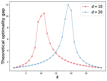
(a) $n=30$

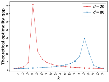
(b) $n=100$

Figure 1: The optimality gaps of RAOD-RII in Corollary 4.18

Corollary 4.19 (Optimality gap)

When $k=d$, RAOD-RI admits the following optimality gap

$$1\leq\frac{z_{k}}{\nu_{k}^{\text{C}}}\leq\min\left\{d,n-d+1\right\}.$$

4.3 The Cutting-Plane Algorithm

Solving RAOD to optimality is computationally expensive. To mitigate this challenge, this subsection presents an exact algorithm designed to enhance existing B&B methods, which typically use the classic lower bound from RAOD-RI (see, e.g., Hendrych et al. 2023). Instead, our approach leverages the formulation (3) with a stronger relaxation, RAOD-RII. Motivated by the convexity of the function $\operatorname{conv}\Gamma$, we can recast (3) as a mixed-integer linear programming (MILP) formulation (4). This reformulation is a well-established technique for mixed-integer nonlinear optimization problems (Duran and Grossmann 1986, Quesada and Grossmann 1992).

$$z_{k}=\min_{w\in{\mathbb{R}}^{+},\bm{x}\in\{0,1\}^{n}}\bigg{\{}w:\sum_{i\in[n]}x_{i}=k,w\geq \operatorname{conv}\Gamma\bigg{(}\sum_{i\in[n]}y_{i}\bm{a}_{i}\bm{a}_{i}^{\top};\lambda\bigg{)}+\frac{d-\tilde{k}}{\lambda}$$ (4)

$$+\bm{g}(\bm{y})^{\top}\left(\bm{x}-\bm{y}\right),\ \ \forall\bm{y}\in\{0,1\}^{n},\sum_{i\in[n]}y_{i}=k\bigg{\}},$$

where $\bm{g}(\bm{y})\in{\mathbb{R}}^{n}$ denotes a (sub)gradient of $\operatorname{conv}\Gamma(\sum_{i\in[n]}y_{i}\bm{a}_{i}\bm{a}_{i}^{\top};\lambda)$ at $\bm{y}$, as defined in Remark 4.15.

However, the problem (4) incorporates an exponentially large number of linear inequalities, which causes computational challenges. To address this, we design a customized cutting plane algorithm for (4) that iteratively adds linear inequalities. The pseudo-code is provided in Algorithm 1. This outer-approximation scheme, as introduced in the seminal work of Duran and Grossmann (1986), was proven to converge optimally for solving MINLPs.

Algorithm 1 The cutting-plane algorithm for (4)

Input: Vectors $\{\bm{a}_{i}\in{\mathbb{R}}^{d}\}_{i\in[n]}$, a constant $\lambda>0$, an integer $k\in[n]$, and target optimality $\epsilon>0$

Initialize $t=1$, $\bm{x}^{t}\in\{0,1\}^{n}$ with $\sum_{i\in[n]}x^{t}_{i}=k$ and $\mbox{UB}=\operatorname{conv}\Gamma\left(\sum_{i\in[n]}x^{t}_{i}\bm{a}_{i}\bm{a}_{i}^{\top};\lambda\right)+\frac{d-\tilde{k}}{\lambda}$

repeat

  Solve the following optimization problem, where $(w^{t+1},\bm{x}^{t+1})$ denotes an optimal solution

$$\min_{\begin{subarray}{c}w\in{\mathbb{R}}_{+},\bm{x}\in\{0,1\}^{n}\\ \sum_{i\in[n]}x_{i}=k\end{subarray}}\bigg{\{}w:w\geq\operatorname{conv}\Gamma\bigg{(}\sum_{i\in[n]}x^{\ell}_{i}\bm{a}_{i}\bm{a}_{i}^{\top};\lambda\bigg{)}+\frac{d-\tilde{k}}{\lambda}+\bm{g}\left(\bm{x}^{\ell}\right)^{\top}\left(\bm{x}-\bm{x}^{\ell}\right),\forall\ell\in[t]\bigg{\}}$$

  Update $\mbox{UB}=\min\left\{\mbox{UB},\operatorname{conv}\Gamma\left(\sum_{i\in[n]}x^{t+1}_{i}\bm{a}_{i}\bm{a}_{i}^{\top};\lambda\right)+\frac{d-\tilde{k}}{\lambda}\right\}$

  Update $t=t+1$

until $\left(w^{t}-\mbox{UB}\right)/\mbox{UB}\leq\epsilon$

Output: $\bm{x}^{t}$ and $w^{t}$

At each iteration of Algorithm 1, a MILP problem over $(w,\bm{x})$, called the master problem, is solved. This subproblem of (4) is based on a subset of linear inequalities. As the number of linear cuts increases, the solution values of $w^{t}$ form a non-decreasing sequence of lower bounds for RAOD. Algorithm 1 terminates when the relative gap between this lower bound (i.e., $w^{t}$) and the best-known upper bound (i.e., UB) reaches a fixed tolerance $\epsilon$. We choose $\epsilon=10^{-4}$ in our experiments. According to Bertsimas et al. (2020), Algorithm 1 can be efficiently implemented in advanced MILP packages (e.g., CPLEX, Gurobi) with the use of lazy constraints and callback functions. However, a time limit is necessary to impose on Algorithm 1, especially when solving large-sized instances. Indeed, as often in mixed-integer optimization, the cutting plane algorithm can quickly find a high-quality solution, but proving its optimality can take much longer. In our experiments, we set a time limit of one hour for Algorithm 1.

We employ several strategies to accelerate the computation of Algorithm 1 in practice. First, we enhance the algorithm using a high-quality warm start obtained from our approximation algorithms in Section 5, instead of randomly initializing a feasible solution. Second, a variable-fixing technique, proposed by Li (2024), is applied to identify some binary variables in (3) that take values of 1 or 0 at optimality. Fixing these variables can reduce the problem size of RAOD while preserving the optimal solution. The effectiveness of this variable-fixing process depends on the strength of the convex relaxations used. Notably, the use of RAOD-RII allows for the fixing of more binary variables. Finally, we solve RAOD-RII before running Algorithm 1 to obtain an initial lower bound. This helps reduce the root gap.

5 The Forward and Backward Greedy Algorithms

In this section, we investigate the scalable forward and backward greedy search strategies and derive their approximation ratios tailored for two different ranges of $k$ in RAOD, specifically for $k\in[d-1]$ and $k\in[d,n]$, respectively.

The forward greedy algorithm begins with an empty set and then iteratively selects the best new data point to add to the set. This process continues until the set reaches a size of $k$. Using the Sherman–Morrison formula, Chamon and Ribeiro (2017b) designed an efficient implementation of forward greedy for solving RAOD, as detailed in Algorithm 2.

Algorithm 2 The forward greedy algorithm for RAOD (Chamon and Ribeiro 2017a)

Input: Vectors $\{\bm{a}_{i}\}_{i\in[n]}\in{\mathbb{R}}^{d}$, a constant $\lambda>0$, and an integer $k\in[n]$

Initialize $S_{F}=\emptyset$ and $\bm{\Lambda}=\frac{1}{\lambda}\bm{I}_{d}$

for $j\in[k]$ do

  Compute $i^{*}=\argmax_{i\in[n]\setminus S_{F}}\frac{\bm{a}_{i}^{\top}\bm{\Lambda}\bm{\Lambda}\bm{a}_{i}}{1+\bm{a}_{i}^{\top}\bm{\Lambda}\bm{a}_{i}}$

  Update $S_{F}=S_{F}\cup\{i^{*}\}$ and $\bm{\Lambda}=\bm{\Lambda}-\frac{\bm{\Lambda}\bm{a}_{i^{*}}\bm{a}_{i^{*}}^{\top}\bm{\Lambda}}{1+\bm{a}_{i^{*}}^{\top}\bm{\Lambda}\bm{a}_{i^{*}}}$

end for

Output: $S_{F}$

The backward greedy algorithm, in contrast to the forward greedy approach, starts with a solution of selecting all data points and then removes an element that results in the smallest objective value at each iteration. The procedure repeats until only $k$ data points are left, which is presented in Algorithm 3. Specifically, at each iteration of Algorithm 3, we have that $\bm{\Lambda}=(\sum_{j\in S_{B}}\bm{a}_{j}\bm{a}_{j}^{\top}+\lambda\bm{I}_{d})^{-1}$, and the goal is to solve

$$\min_{i\in S_{B}}f(S_{B}\setminus\{i\})=\min_{i\in S_{B}}\operatorname{tr}\left(\bm{\Lambda}+\frac{\bm{\Lambda}\bm{a}_{i}\bm{a}_{i}^{\top}\bm{\Lambda}}{1-\bm{a}_{i}^{\top}\bm{\Lambda}\bm{a}_{i}}\right)=f(S_{B})+\min_{i\in S_{B}}\frac{\bm{a}_{i}^{\top}\bm{\Lambda}\bm{\Lambda}\bm{a}_{i}}{1-\bm{a}_{i}^{\top}\bm{\Lambda}\bm{a}_{i}},$$

where the first equation results from the Sherman–Morrison formula. Similarly, we update the matrix $\bm{\Lambda}$ by the Sherman–Morrison formula.

Algorithm 3 The backward greedy algorithm for RAOD

Input: Vectors $\{\bm{a}_{i}\}_{i\in[n]}\in{\mathbb{R}}^{d}$, a constant $\lambda>0$, and an integer $k\in[n]$

Initialize $S_{B}=[n]$ and $\bm{\Lambda}=(\sum_{j\in S_{B}}\bm{a}_{j}\bm{a}_{j}^{\top}+\lambda\bm{I}_{d})^{-1}$

for $j\in[n-k]$ do

  Compute $i^{*}=\argmin_{i\in S_{B}}\frac{\bm{a}_{i}^{\top}\bm{\Lambda}\bm{\Lambda}\bm{a}_{i}}{1-\bm{a}_{i}^{\top}\bm{\Lambda}\bm{a}_{i}}$

  Update $S_{B}=S_{B}\setminus\{i^{*}\}$ and $\bm{\Lambda}=\bm{\Lambda}+\frac{\bm{\Lambda}\bm{a}_{i^{*}}\bm{a}_{i^{*}}^{\top}\bm{\Lambda}}{1-\bm{a}_{i^{*}}^{\top}\bm{\Lambda}\bm{a}_{i^{*}}}$

end for

Output: $S_{B}$

Using Lemma 3.2, we guarantee the theoretical performance for Algorithms 2 and 3.

Theorem 5.1 (Approximation ratios and complexities)

For $k\in[d-1]$, Algorithm 2 enjoys a-$\frac{d-1}{d-k}$ approximation ratio, that is,

$$f(S_{F})\leq\frac{d-1}{d-k}z_{k}.$$

For $k\in[d,n]$, Algorithm 3 enjoys a-$\frac{n-d+1}{k-d+1}$ approximation ratio, that is,

$$f(S_{B})\leq\frac{n-d-1}{k-d+1}z_{k}.$$

In addition, the running time complexities of Algorithms 2 and 3 are ${\mathcal{O}}(knd^{2})$ and ${\mathcal{O}}((n-k)nd^{2})$, respectively.

Proof 5.2

Proof. See Appendix 8.14. $\square$

We remark on Theorem 5.1 that

1. The forward greedy Algorithm 2 has been extensively studied in the Bayesian AOD literature (see, Chamon and Ribeiro 2017a, Bian et al. 2017). Theorem 5.1 offers the first-known data-independent approximation ratio for Algorithm 2 when applied to RAOD with $k\in[d-1]$;

2. We develop the novel backward greedy Algorithm 3 that delivers an approximation ratio when $k\in[d,n]$;

3. As a classical intuition, forward greedy is effective when selecting a small number of data points, while backward greedy becomes more efficient as the selection size grows. Theorem 5.1 rigorously validates this intuition, as it offers theoretical guarantees for Algorithms 2 and 3 in the small- and large-$k$ ranges, respectively, as illustrated in Figure 2; and

4. Finally, we consider Algorithm 4 to select the better solution between the outputs of Algorithms 2 and 3, which yields a high-quality solution to RAOD for all values of $k$.

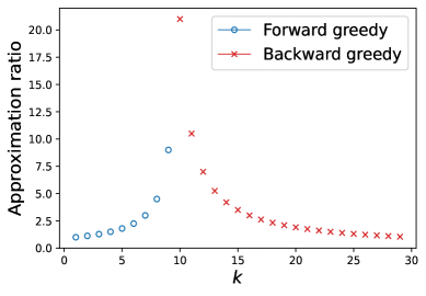
(a) $d=10$

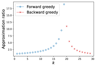
(b) $d=20$

Figure 2: The approximation ratios of Algorithms 2 and 3 in Theorem 5.1 with $n=30$

Algorithm 4 The combination of the forward and backward greedy algorithms for RAOD

Input: Vectors $\{\bm{a}_{i}\}_{i\in[n]}\in{\mathbb{R}}^{d}$, a constant $\lambda>0$, and an integer $k\in[n]$

Denote by $S_{F}$ the output of Algorithm 2

Denote by $S_{B}$ the output of Algorithm 3

Output: The better solution between $S_{F}$ and $S_{B}$

Corollary 5.3

Algorithm 4 has an approximation ratio of $\frac{d-1}{d-k}$ for $k\in[d-1]$, and $\frac{n-d+1}{k-d+1}$ for $k\in[d,n]$. In addition, its time complexity is ${\mathcal{O}}(n^{2}d^{2})$.

6 Numerical Results

This section evaluates the numerical performance of our formulations and algorithms developed for solving RAOD. The computational results not only demonstrate the efficiency of our approaches but also provide empirical support for our theoretical findings. All the experiments enforce a 1-hour timeout, and are conducted in Python 3.6 with calls to Gurobi 9.5.2 on a PC with 10-core CPU, 16-core GPU, and 16GB of memory. We begin by introducing the datasets, both synthetic and real, used in our computational experiments.

Synthetic data. Given $(n,d)$, we randomly generate a data matrix $\bm{A}\in{\mathbb{R}}^{d\times n}$ by a normal distribution $\mathcal{N}(0,1)$, and let $\bm{a}_{i}$ be the $i$-th column of $\bm{A}$ for each $i\in[n]$.

UCI data (Blake 1998). We further conduct experiments on five UCI datasets- autos, breastcancer, sml, gas, and song, with dimensions $(n,d)$ of $(159,24)$, $(194,33)$, $(200,22)$, $(500,128)$, and $(1000,90)$, respectively. We begin by removing all-zero columns from the data matrix. For datasets with a huge number of observations, we randomly sample a manageable subset of $n$ data points to ensure computational feasibility when testing exact methods. Finally, we apply min-max normalization to each feature (i.e., each row) of the resulting matrix $\bm{A}\in{\mathbb{R}}^{d\times n}$, so that it falls within the range $[0,1]$.

Movie rating data (Dooms et al. 2013). The movie rating dataset is used to demonstrate an application of RAOD to the new user cold-start problem in recommendation systems. The dataset consists of ratings provided by 71,707 users for a total of 38,018 movies. Ratings are shifted from the range [0, 10] to [1, 11] by adding one to each rating to avoid zero vectors.

6.1 Evaluations of Convex Relaxations

This subsection evaluates the three convex relaxations: RAOD-RI, AMESP-R, and RAOD-RII, by comparing their optimality gaps and computation times with varying-scale instances. We use the Frank-Wolfe algorithm to solve them. The results are summarized in Figures 3 and 4. For each convex relaxation, we compute “Gap (%)” by $100\times(\text{upper bound}-\text{relaxation bound})/\text{upper bound}$, where the upper bound of RAOD is obtained from Algorithm 4. Our results verify the effectiveness of RAOD-RII and its dominance over RAOD-RI and AMESP-R.

We first test three synthetic datasets with $n=100$ and different values of $d,\lambda$, where for each dataset, we consider $k\in\{5,10,\cdots,95\}$. As Figure 3 below shows, RAOD-RII delivers the tightest lower bound. It is worth noting that the gap curves for RAOD-RII in Figures 3(a), 3(b) and 3(c) closely match the theoretical gaps shown in Figure 1, where the maximum occurs near $k=d$. Besides, we would like to comment on the gaps of RAOD-RI and AMESP-R in two ranges of $k$ based on Figures 3(a), 3(b) and 3(c). We see that for $k<d$, AMESP-R outperforms RAOD-RI. When $k\geq d+1$, RAOD-RI and RAOD-RII are identical, and they dominate AMESP-R, as demonstrated in Theorem 4.16. In fact, AMESP-R produces extremely large gaps for $k\in[d+1,n]$, often exceeding $100\%$, which indicates that it returns a negative lower bound. This phenomenon aligns with our result in Part (ii) of Theorem 3.7. As seen from the differences between Figures 3(a) and 3(b), increasing $d$ tends to improve AMESP-R and RAOD-RII but worsen RAOD-RI, especially for small-$k$ instances. Finally, we find that AMESP-R requires the largest computation time since it builds on the $n\times n$ matrix space.

In Figure 4, we test the relaxations of RAOD on three larger-sized real datasets ($n=159,200,1000$) with $\lambda=1$. The values of $k$ are tested in increments of 5 for $n=159,200$, and larger increments of 50 for $n=1000$. As before, RAOD-RII wins on all test instances. We observe in Figures 4(a), 4(b) and 4(c) that as $k\to d$ from below, RAOD-RII strictly outperforms RAOD-RI and AMESP-R even if we combine them and take the minimum. It is still obvious that the gap pf RAOD-RII tends to be larger when $k$ approaches $d$ from either side. Interestingly, as we observe in Figures 4(a) and 4(b), RAOD-RI and AMESP-R are no longer directly comparable for values of $k<d$. For the largest test case in Figure 4(f), where $n=1000$, AMESP-R hits the time limit, highlighting its scalability limitations.

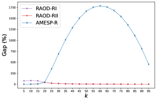
(a) Gap for $(n,d,\lambda)=(100,20,1)$

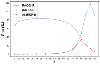
(b) Gap for $(n,d,\lambda)=(100,80,1)$

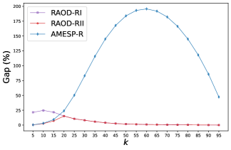
(c) Gap for $(n,d,\lambda)=(100,20,10)$

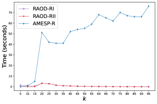
(d) Time for $(n,d,\lambda)=(100,20,1)$

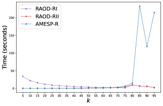
(e) Time for $(n,d,\lambda)=(100,80,1)$

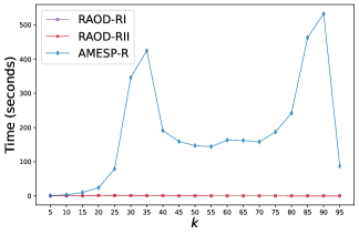
(f) Time for $(n,d,\lambda)=(100,20,10)$

Figure 3: Convex relaxations of RAOD: Gaps and computation times on synthetic data

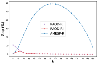
(a) Gap for $(n,d,\lambda)=(159,24,1)$

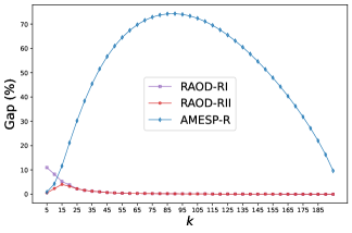
(b) Gap for $(n,d,\lambda)=(200,22,1)$

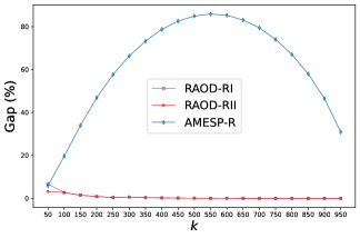
(c) Gap for $(n,d,\lambda)=(1000,90,1)$

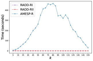
(d) Time for $(n,d,\lambda)=(159,24,1)$

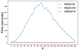
(e) Time for $(n,d,\lambda)=(200,22,1)$

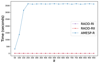
(f) Time for $(n,d,\lambda)=(1000,90,1)$

Figure 4: Convex relaxations of RAOD: Gaps and computation times on real data

6.2 Evaluations of Approximation Algorithms

In this subsection, we evaluate the performance of several approximation algorithms for solving RAOD on the same data instances. Specifically, we compare our Algorithms 2 and 3 with the following methods: “LocalSearch,” referring to the local search algorithm proposed by Li and Xie (2024) for AMESP; “RegVol,” the regularized volume sampling algorithm introduced by Dereziński and Warmuth (2017); and its more efficient implementation “FastRegVol.” Local search starts from a random solution, and sampling algorithms are run 20 times per instance, with the best result reported. Notably, we omit comparisons with the randomized sampling algorithms from Li and Xie (2024), Tantipongpipat (2020), as they were computationally intensive and failed to finish within one hour on these instances.

The approximation gaps and computation times for the evaluated algorithms are summarized in Figures 5 and 6. We track the best lower bound $\nu_{k}^{\text{N}}$ found from the previous subsection, and compute “Gap (%)” by $100\times(\text{upper bound}-\nu_{k}^{\text{N}})/\text{upper bound}$, where the upper bound is the objective value returned by each approximation method. We observe that combinatorial algorithms outperform the two sampling algorithms, with significant improvements when $k>d$ and $d$ is relatively small compared to $n$. The comparison of Figures 5(d) and 5(e) shows that the runtime of FastRegVol increases more rapidly as $d$ increases, compared to the other algorithms. Across all algorithms, the largest approximation gaps tend to occur near $k=d$. This may result from using a lower bound $\nu_{k}^{\text{N}}$ rather than the true optimal value in computing the gap, as RAOD-RII deviates most from the optimum around $k=d$ (see Figures 3 and 4). In general, the three combinatorial algorithms are not directly comparable, but the local search algorithm outperforms our greedy Algorithms 2 and 3 in more cases. However, for the largest instance with $n=1000$ in Figures 6(c) and 6(f), it takes considerably longer but achieves nearly identical gaps to our algorithms. In summary, our Algorithms 2 and 3 strike the best balance between scalability and solution quality among all the algorithms. As seen in Figure 6(b), Algorithm 2 yields a smaller gap when $k$ is small, while Algorithm 3 becomes more effective when $k\geq d$. This trend aligns with their theoretical guarantees discussed following Theorem 5.1.

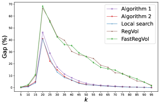
(a) Gap for $(n,d,\lambda)=(100,20,1)$

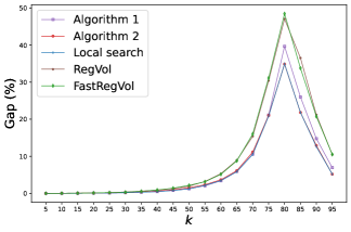
(b) Gap for $(n,d,\lambda)=(100,80,1)$

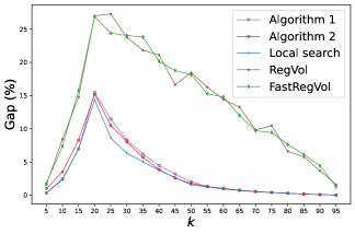
(c) Gap for $(n,d,\lambda)=(100,20,10)$

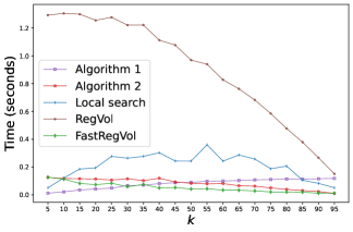
(d) Time for $(n,d,\lambda)=(100,20,1)$

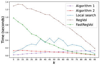
(e) Time for $(n,d,\lambda)=(100,80,1)$

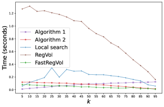
(f) Time for $(n,d,\lambda)=(100,20,10)$

Figure 5: Approximation algorithms of RAOD: Gaps and computation times on synthetic data

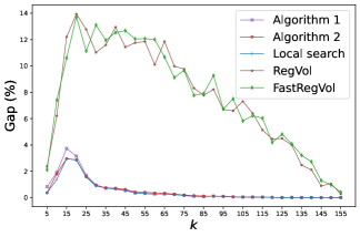
(a) Gap for $(n,d,\lambda)=(159,24,1)$

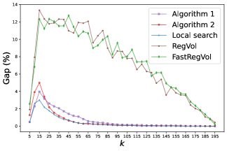
(b) Gap for $(n,d,\lambda)=(200,22,1)$

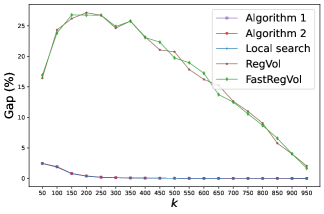
(c) Gap for $(n,d,\lambda)=(1000,90,1)$

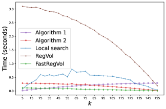
(d) Time for $(n,d,\lambda)=(159,24,1)$

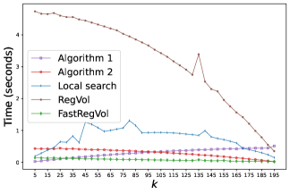
(e) Time for $(n,d,\lambda)=(200,22,1)$

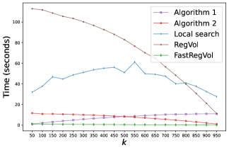
(f) Time for $(n,d,\lambda)=(1000,90,1)$

Figure 6: Approximation Algorithms of RAOD: Gaps and computation times on real data

6.3 Performance of Exact Algorithms

We now compare the three (mixed-)integer convex formulations introduced in Sections 3 and 4 using both synthetic and real datasets. To solve our proposed formulation (3), we develop the cutting-plane Algorithm 1, which we implement using Gurobi’s lazy constraints. The same cutting-plane scheme can be readily extended to (1), since its objective function is also convex; we refer to this variant as “Cutting plane via (1).” For fairness, both algorithms employ the same computational enhancements and termination criterion, as detailed in Subsection 4.3. In addition, we use Gurobi to solve the formulation MISOCP directly. Although AMESP-R offers an exact formulation when $\bm{x}$ is binary, we do not include it in our comparison due to its high computational cost and the fact that RAOD-RII theoretically dominates AMESP-R (see Theorem 4.16, Part (iii)).

We restrict our experiments to the case $k<d$. From a theoretical perspective, the objective functions of (1) and (3) are equivalent when $k\geq d$, as indicated by Lemma 4.11, making the comparison trivial. From a practical perspective, this choice is also well-motivated. In high-dimensional application problems such as user cold-start recommendation systems, constraints such as limited budgets or user cognitive costs naturally enforce small values of $k$ (Chamon and Ribeiro 2017a).

For each instance with the fixed pair $(n,d)$, we vary the parameters $\lambda\in\{1,10\}$ and $k\in\{5,10\}$, thus creating four testing cases. The numerical results are presented in Tables 3 and 4, where “MIPGap(%)” represents the relative optimality gap in percentage at which Gurobi terminates. A MIPGap of $0.00$ indicates a certified optimal solution. Among the three exact algorithms, the cutting-plane algorithm based on (1) attains the largest MIPGaps in most instances and only occasionally reaches optimality when $\lambda=10$, as seen in Table 4. MISOCP also struggles with large MIPGaps and timeouts. In particular, for instances with $n\geq 500$, MISOCP may even exhaust available memory, marked by “–” in Table 4. In contrast, our proposed Algorithm 1 achieves significantly smaller MIPGaps and solves most cases to optimality within 1 hour, especially for $k=5$. These results show the superiority of Algorithm 1 in both computational efficiency and MIPGap reduction for the tested instances, which can be primarily attributed to the strength of the continuous relaxation of (3). For small $k<d$, its relaxation RAOD-RII is strictly tighter than RAOD-RI, the continuous relaxation of (1) and MISOCP.

Next, we would like to comment on the effect of parameters $d$, $k$, and $\lambda$. What is interesting in Table 3 is that, for fixed $n,k,\lambda$, the MIPGap for Algorithm 1 decreases as the experimental dimension $d$ increases. For instance, Algorithm 1 solves the case with $(n,d,k,\lambda)=(100,80,10,1)$ in just $7$ seconds, whereas the lower-dimensional case $(100,20,10,1)$ takes longer than $1$ hour. A likely explanation is that, according to Corollary 4.18 and the discussion following Theorem 3.7, RAOD-RII admits an optimality gap of $(d-1)/(d-k)$ when $k\leq(n+1)/2$. Since this theoretical gap is decreasing with $d$ (for fixed $k$), RAOD-RII becomes tighter in higher dimensions, thus enhancing the performance of Algorithm 1. This observation highlights the advantage of our Algorithm 1 in complex, high-dimensional problems. As expected, instances with $k=10$ are harder to solve than those with $k=5$. We also observe that “Cutting plane via (1)” and MISOCP benefit from higher $\lambda$ but still fail to close the gap in many instances. In contrast, the effect of $\lambda$ on the performance of Algorithm 1 is instance-dependent. Table 3 shows that the case with $\lambda=10$ poses larger MIPGaps for Algorithm 1 than the case with $\lambda=1$, whereas in Table 4, the opposite holds.

Finally, we evaluate the approximation quality of Algorithm 4 by comparing its outputs with the best lower bounds returned by Algorithm 1. As shown in the “Gap(%)” column of Tables 3 and 4, this gap remains within $2.45\%$ and is computed in under $11$ seconds, which demonstrates both the scalability and near-optimality of Algorithm 4. Moreover, in cases where this gap is smaller than the MIPGap of Algorithm 1, it indicates that Algorithm 1 failed to find a better feasible solution within the time limit than the one produced by Algorithm 4.

Table 3: Exact algorithms for RAOD on synthetic data

Dataset	Params		Cutting plane via (1)		MISOCP		Algorithm 1 via (3)		Algorithm 4
($n$, $d$)	$\lambda$	$k$	MIPGap(%)	Time	MIPGap(%)	Time	MIPGap(%)	Time	Gap(%)	Time
(100, 20)	1	5	77.92	3600	76.08	3600	0.00	589	0.02	1
	1	10	82.54	3600	80.14	3600	0.82	3600	0.88	1
	10	5	21.17	3600	18.15	3600	0.00	6	0.04	1
	10	10	27.70	3600	22.63	3600	2.65	3600	2.45	1
(100, 50)	1	5	75.43	3600	73.18	3600	0.00	1	0.00	1
	1	10	83.57	3600	81.80	3600	0.04	3600	0.03	1
	10	5	25.80	3600	22.25	3600	0.00	1	0.00	1
	10	10	36.68	3600	31.40	3600	0.25	3600	0.23	1
(100, 80)	1	5	69.19	3600	66.73	3600	0.00	1	0.00	1
	1	10	78.01	3600	75.20	3600	0.00	7	0.00	1
	10	5	25.78	3600	23.60	3600	0.00	1	0.00	1
	10	10	36.04	3600	32.57	3600	0.07	3600	0.06	1
(150, 20)	1	5	79.95	3600	78.40	3600	0.00	8	0.00	1
	1	10	84.63	3600	82.14	3600	0.47	3600	0.59	1
	10	5	23.41	3600	21.88	3600	0.00	2	0.00	1
	10	10	30.58	3600	24.48	3600	1.79	3600	1.65	1
(150, 50)	1	5	78.67	3600	76.91	3600	0.00	1	0.00	1
	1	10	86.36	3600	85.03	3600	0.02	3600	0.02	1
	10	5	28.07	3600	25.79	3600	0.00	1	0.00	1
	10	10	39.70	3600	35.77	3600	0.11	3600	0.11	1
(150, 80)	1	5	75.18	3600	73.05	3600	0.00	1	0.00	1
	1	10	83.70	3600	82.13	3600	0.00	1	0.00	1
	10	5	28.69	3600	25.63	3600	0.00	1	0.00	1
	10	10	40.13	3600	36.23	3600	0.04	3600	0.04	1

Table 4: Exact algorithms for RAOD on real data

Dataset	Params		Cutting plane via (1)		MISOCP		Algorithm 1 via (3)		Algorithm 4
($n$, $d$)	$\lambda$	$k$	MIPGap(%)	time	MIPGap(%)	time	MIPGap(%)	time	Gap(%)	time
(159, 24)	1	5	13.10	3600	8.49	3600	0.00	3548	0.02	1
	1	10	16.14	3600	6.86	3600	1.64	3600	1.80	1
	10	5	0.00	19	0.27	3600	0.00	4	0.04	1
	10	10	0.12	3600	0.27	3600	0.06	3600	0.06	1
(194, 33)	1	5	6.65	3600	5.93	3600	0.00	119	0.12	1
	1	10	9.64	3600	3.92	3600	1.15	3600	1.23	1
	10	5	0.00	2	0.01	3600	0.00	1	0.00	1
	10	10	0.00	28	0.11	3600	0.00	3	0.00	1
(200, 22)	1	5	16.08	3600	0.46	3600	0.00	416	0.08	1
	1	10	19.70	3600	2.27	3600	2.43	3600	2.27	1
	10	5	0.00	47	0.10	3600	0.00	1	0.14	1
	10	10	0.24	3600	0.24	3600	0.08	3600	0.11	1
(500, 128)	1	5	2.90	3600	–	–	0.00	48	0.02	3
	1	10	1.91	3600	–	–	0.00	441	0.01	3
	10	5	0.00	30	–	–	0.00	1	0.00	3
	10	10	0.00	26	–	–	0.00	1	0.00	3
(1000, 90)	1	5	9.15	3600	–	–	0.00	192	0.00	11
	1	10	20.05	3600	–	–	0.10	3600	0.10	11
	10	5	0.00	2181	–	–	0.00	4	0.01	11
	10	10	0.37	3600	–	–	0.00	26	0.00	11

6.4 Application to User Cold-Start Recommendation

This subsection presents an application of RAOD to the user cold-start recommendation problem introduced in Section 1. Recall that the system struggles with predicting preferences for new users without prior ratings. A common solution is to select a small, representative set of items for new users to rate. The criterion for selection usually relies on a statistical measure aimed at minimizing the model mean squared error, most notably A-optimality and D-optimality (see, e.g., Chamon and Ribeiro 2017a, Rubens et al. 2009, Zhao and Wang 2015). These correspond to RAOD and regularized DOD optimization problems. In the following, we compare the performance of RAOD, regularized DOD, and a random selection baseline in addressing the cold-start problem. We apply the widely-used forward greedy algorithm to solve both RAOD and regularized DOD for a fair comparison (Krause et al. 2008).

To understand a new user’s movie preferences, we leverage the intuition that their tastes are related to how existing (training) users have rated the same movies (Deldjoo et al. 2019). For each movie $i\in[n]$, the vector $\bm{a}_{i}\in{\mathbb{R}}^{d}$ contains its ratings from $d$ training users. As done in Chamon and Ribeiro (2017a), we assume that the new user’s ratings can be expressed as a linear combination of the past rating data, modeled as $\bm{A}^{\top}\bm{\theta}$, where $\bm{\theta}\in{\mathbb{R}}^{d}$ captures how similar the new user is to each training user. Since $\bm{\theta}$ is unknown, we select a subset $\widehat{S}\subseteq[n]$ of $k$ movies for the new user to rate, aiming to provide maximal information for estimating $\bm{\theta}$. With the estimate $\widehat{\bm{\theta}}$, we predict the new user’s ratings for the remaining $(n-k)$ movies as $\bm{a}_{i}^{\top}\widehat{\bm{\theta}}$ for all $i\in[n]\setminus\widehat{S}$. Finally, we evaluate the quality of the selected subset $\widehat{S}$ by computing the mean squared error (MSE) between predicted and actual ratings. A lower MSE indicates that the selected movies more effectively capture the new user’s preferences.

To facilitate testing, we truncate the movie rating data from Dooms et al. (2013) by randomly selecting a subset of ratings. Specifically, for a fixed number of movies, training users, and new users, we repeat the truncation process 15 times with different random seeds. Tables 6 and 6 compare the average MSE across all 20 and 50 new users using the three selection methods. To be specific, the average MSE is computed by averaging per-seed MSEs of all new users and then averaging these values across 15 random seeds. We refer to the MSE values based on our RAOD method, regularized DOD, and random selection as “A-MSE”, “D-MSE”, and “R-MSE”, respectively. For each dataset, we vary the regularization parameter $\lambda\in\{0.5,1,1.5\}$. The random selection method is clearly unaffected by the choice of $\lambda$. Across all experimental settings, RAOD consistently yields the lowest or comparable MSE. In contrast, while the D-optimality-based method occasionally outperforms RAOD in Table 6, it tends to generate extremely high MSE in larger-scale settings with 50 new users, as shown in Table 6 where $n=700$. The random selection method performs the worst overall, particularly in Table 6. These results highlight the robustness and effectiveness of the RAOD-based selection for cold-start recommendations, particularly as the number of new users grows.

Table 5: The average MSE of 20 new users

$(n,d,k)$	$\lambda$	A-MSE	D-MSE	R-MSE
(500, 100, 20)	0.5	0.0346	0.2430	0.0460
	1	0.0346	0.2430	0.0460
	1.5	0.0346	0.2435	0.0460
(600, 100, 20)	0.5	0.0368	0.0517	0.0463
	1	0.0368	0.1864	0.0463
	1.5	0.0386	0.1950	0.0463
(700, 100, 20)	0.5	0.0364	0.0360	0.0450
	1	0.0361	0.0357	0.0450
	1.5	0.0353	0.0351	0.0450
(800, 100, 20)	0.5	0.0366	0.0382	0.0466
	1	0.0367	0.0383	0.0466
	1.5	0.0378	0.0454	0.0466
(900, 100, 20)	0.5	0.0383	0.0385	0.0483
	1	0.0390	0.0384	0.0483
	1.5	0.0391	0.0382	0.0483

Table 6: The average MSE of 50 new users

$(n,d,k)$	$\lambda$	A-MSE	D-MSE	R-MSE
(500, 150, 50)	0.5	0.0323	0.0355	1.65e+26
	1	0.0343	0.0355	1.65e+26
	1.5	0.0343	0.0381	1.65e+26
(600, 150, 50)	0.5	0.0388	0.0578	2.35e+26
	1	0.0398	0.0737	2.35e+26
	1.5	0.0392	0.0752	2.35e+26
(700, 150, 50)	0.5	0.0354	1.72e+21	2.00e+26
	1	0.0354	1.72e+21	2.00e+26
	1.5	0.0356	1.72e+21	2.00e+26
(800, 150, 50)	0.5	0.0366	0.0993	3.54e+26
	1	0.0367	0.1179	3.54e+26
	1.5	0.0367	0.1182	3.54e+26
(900, 150, 50)	0.5	0.0361	0.0355	1.23e+26
	1	0.0361	0.0425	1.23e+26
	1.5	0.0361	0.0480	1.23e+26

7 Conclusion

We study the regularized A-optimal design (RAOD) problem and prove its NP-hardness for the first time. A key insight from our results is that the performance of both formulations and algorithms for RAOD hinges on whether the selection size $k$ exceeds the data dimension $d$. Specifically, we demonstrate that the two existing relaxations perform well in only one of the two ranges ($k\leq d-1$ or $k\geq d$), but poorly in the other. To address this, we propose a novel convex integer formulation that yields a stronger relaxation with provable performance guarantees for all $k$. This formulation significantly accelerates the exact cutting-plane algorithm in small-$k$ and high-dimensional settings. We further investigate the complementary forward and backward greedy algorithms, tailored respectively to the ranges $k\leq d-1$ and $k\geq d$. Our numerical experiments demonstrate the effectiveness and efficiency of the proposed algorithms. Our work can be seen as a non-sequential experimental design scheme, where the data points are selected at once. A possible future direction is to explore adaptive strategies that select points sequentially based on prior selections.

8 Additional proof

8.1 Proof of Proposition 2.1

Proof 8.1

Proof. We prove the result by showing that the objective functions of RAOD and AMESP are equivalent. For any solution $S$ of RAOD, let $\sigma_{1}\geq\cdots\geq\sigma_{d}\geq 0$ and $\beta_{1}\geq\cdots\geq\beta_{k}\geq 0$ denote the eigenvalues of $\bm{A}_{S}\bm{A}_{S}^{\top}\in{\mathcal{S}}_{+}^{d}$ and $\bm{A}_{S}^{\top}\bm{A}_{S}\in{\mathcal{S}}_{+}^{k}$, respectively. Then, our analysis is split into two parts depending on whether $k\leq d$ holds or not.

1. $k\in[d]$. Because $\bm{A}_{S}\bm{A}_{S}^{\top}\in{\mathcal{S}}_{+}^{d}$ and $\bm{A}_{S}^{\top}\bm{A}_{S}\in{\mathcal{S}}_{+}^{k}$ admit the same nonzero eigenvalues, their eigenvalues satisfy $\sigma_{i}=\beta_{i}$ for any $i\in[k]$ and $\sigma_{i}=0$ for all $i\in[k+1,d]$. Given this, we have that

   $$f(S) =\operatorname{tr}\left(\left(\bm{A}_{S}\bm{A}_{S}^{\top}+\lambda\bm{I}_{d}\right)^{-1}\right)=\sum_{i\in[d]}\frac{1}{\sigma_{i}+\lambda}=\sum_{i\in[k]}\frac{1}{\beta_{i}+\lambda}+\frac{d-k}{\lambda}$$

   $$=\operatorname{tr}\left(\left(\bm{A}_{S}^{\top}\bm{A}_{S}+\lambda\bm{I}_{k}\right)^{-1}\right)+\frac{d-k}{\lambda}=\operatorname{tr}\left(\left(\bm{C}_{S,S}\right)^{-1}\right)+\frac{d-k}{\lambda},$$

   where the first and the last equations follow from the definitions of $\bm{A}$ and $\bm{C}$, respectively.

2. $k\in[d+1,n]$. Analogously, according to the relation of the eigenvalues between $\bm{A}_{S}\bm{A}_{S}^{\top}\in{\mathcal{S}}_{+}^{d}$ and $\bm{A}_{S}^{\top}\bm{A}_{S}\in{\mathcal{S}}_{+}^{k}$, we get $\sigma_{i}=\beta_{i}$ for any $i\in[d]$ and $\beta_{i}=0$ for all $i\in[d+1,k]$. Then, we have that

   $$f(S) =\operatorname{tr}\left(\left(\bm{A}_{S}\bm{A}_{S}^{\top}+\lambda\bm{I}_{d}\right)^{-1}\right)=\sum_{i\in[d]}\frac{1}{\sigma_{i}+\lambda}=\sum_{i\in[k]}\frac{1}{\beta_{i}+\lambda}-\frac{k-d}{\lambda}$$

   $$=\operatorname{tr}\left(\left(\bm{A}_{S}^{\top}\bm{A}_{S}+\lambda\bm{I}_{k}\right)^{-1}\right)+\frac{d-k}{\lambda}=\operatorname{tr}\left(\left(\bm{C}_{S,S}\right)^{-1}\right)+\frac{d-k}{\lambda}.$$

   We thus complete the proof. $\square$

8.2 Proof of Theorem 2.5

Proof 8.2

Proof. In order to prove the result, we reduce the NP-hard independent set decision problem to AMESP. Given a simple undirected graph $G([n],E)$, we define a symmetric matrix $\bm{C}$ as

$$C_{ij}=\begin{cases}n&\text{if }i=j;\\ 1&\text{if }(i,j)\in E;\\ 0&\text{Otherwise}.\end{cases}$$

For all $i\in[n]$, it is easy to verify that $C_{ii}=n>n-1\geq\sum_{j\neq i}|C_{ij}|$, implying that $\bm{C}$ is a strictly diagonally dominant matrix. Hence, the matrix $\bm{C}$ is positive definite, and so is any principal submatrix of $\bm{C}$. Besides, we can express $\bm{C}=\bm{A}\bm{A}^{\top}+\lambda\bm{I}_{n}$ in the form of the objective matrix in AMESP, where $\lambda$ equals the smallest eigenvalue of $\bm{C}$, and $\bm{A}$ denotes the Cholesky factor of $\bm{C}-\lambda\bm{I}_{n}$. Therefore, the resulting pair $(\bm{A},\lambda)$ can be used as an input instance of RAOD such that RAOD is equivalent to AMESP.

For any subset $S\subseteq[n]$, the subgragh $G_{S}$ comprises the vertices $S$ and edges in the set $E\cap(S\times S)$, and then, the subgragh $G_{S}$ can be represented by the principal submatrix $\bm{C}_{S,S}$.

Next, for a subset $S$ of size $k$, we compute the trace of the inverse of $\bm{C}_{S,S}$ in two cases.

1. If $S$ is a sized-$k$ independent set for the graph $G$, according to the property of independent sets, the resulting subgraph $G_{S}$ has no edges, that is, $(i,j)\notin E$ for any two vertices $i,j$ in $S$. Therefore, the corresponding submatrix $\bm{C}_{S,S}$ to $G_{S}$ must be diagonal, and we can easily compute $\operatorname{tr}((\bm{C}_{S,S})^{-1})=\sum_{i\in S}1/C_{ii}=k/n$.

2. If $S$ is not a sized-$k$ independent set, then, unlike Part (i), there is at least one nonzero off-diagonal entry in $\bm{C}_{S,S}$. Suppose that the vector $\bm{\sigma}\in{\mathbb{R}}_{++}^{k}$ contains the eigenvalues of $\bm{C}_{S,S}$. It follows that

   $$\|\bm{C}_{S,S}\|_{F}^{2}=\sum_{i\in[k]}\sigma_{i}^{2}=\sum_{i\in S}\sum_{j\in S}C_{ij}^{2}\geq kn^{2}+2.$$

   In addition, we have that $\sum_{i\in[k]}\sigma_{i}=\operatorname{tr}(\bm{C}_{S,S})=kn$. As a result, not all entries of $\bm{\sigma}$ can be equal. Otherwise, we would find that $\sum_{i\in[k]}\sigma_{i}^{2}=kn^{2}$, a contradiction with the inequality above.

   According to Lemma 2.4, we get

   $$\frac{k}{\operatorname{tr}((\bm{C}_{S,S})^{-1})}=\frac{k}{\sum_{i\in[k]}\frac{1}{\sigma_{i}}}<\frac{\sum_{i\in[k]}\sigma_{i}}{k}=n\ \ \Longrightarrow\ \ \operatorname{tr}((\bm{C}_{S,S})^{-1})>\frac{k}{n},$$

   where the first inequality is strict because the entries of $\bm{\sigma}$ are not all equal.

By combining the results in Parts (i) and (ii), we conclude that if AMESP yields an optimal value of $k/n+(d-k)/\lambda$, then there exists an independent set of size $k$ in the graph $G$. On the other hand, if the optimal value is larger than $k/n+(d-k)/\lambda$, the independent set decision problem is false. We thus complete the proof. $\square$

8.3 Proof of Lemma 3.2

Proof 8.3

Proof. For each $i\in S$, let us consider the following probability to sample $i$ out of $S$, proposed by Dereziński and Warmuth (2017):

$${\mathbb{P}}(i|S)=\frac{1-\bm{a}_{i}^{\top}\left(\bm{A}_{S}\bm{A}_{S}^{\top}+\lambda\bm{I}_{d}\right)^{-1}\bm{a}_{i}}{s-\operatorname{tr}\left(\bm{A}_{S}^{\top}\left(\bm{A}_{S}\bm{A}_{S}^{\top}+\lambda\bm{I}_{d}\right)^{-1}\bm{A}_{S}\right)}.$$

It is easy to verify that $\sum_{i\in S}{\mathbb{P}}(i|S)=1$. Then, the expected function value of removing an element from $S$ is equal to

$${\mathbb{E}}\left[f(S\setminus\{i\})\right] =\sum_{i\in S}{\mathbb{P}}(i|S)f(S\setminus\{i\})=\sum_{i\in S}{\mathbb{P}}(i|S)\operatorname{tr}\left(\left(\bm{A}_{S}\bm{A}_{S}^{\top}-\bm{a}_{i}\bm{a}_{i}^{\top}+\lambda\bm{I}_{d}\right)^{-1}\right)$$ (5)

$$=\sum_{i\in S}{\mathbb{P}}(i|S)\left(f(S)+\frac{\bm{a}_{i}^{\top}\left(\bm{A}_{S}\bm{A}_{S}^{\top}+\lambda\bm{I}_{d}\right)^{-2}\bm{a}_{i}}{1-\bm{a}_{i}^{\top}\left(\bm{A}_{S}\bm{A}_{S}^{\top}+\lambda\bm{I}_{d}\right)^{-1}\bm{a}_{i}}\right)$$

$$=f(S)+\frac{\operatorname{tr}\left(\bm{A}_{S}^{\top}\left(\bm{A}_{S}\bm{A}_{S}^{\top}+\lambda\bm{I}_{d}\right)^{-2}\bm{A}_{S}\right)}{s-\operatorname{tr}\left(\bm{A}_{S}^{\top}\left(\bm{A}_{S}\bm{A}_{S}^{\top}+\lambda\bm{I}_{d}\right)^{-1}\bm{A}_{S}\right)}$$

$$=f(S)\left(1+\frac{\operatorname{tr}\left(\left(\bm{A}_{S}\bm{A}_{S}^{\top}+\lambda\bm{I}_{d}\right)^{-2}\bm{A}_{S}\bm{A}_{S}^{\top}\right)}{\operatorname{tr}\left(\left(\bm{A}_{S}\bm{A}_{S}^{\top}+\lambda\bm{I}_{d}\right)^{-1}\right)\left(s-\operatorname{tr}\left(\left(\bm{A}_{S}\bm{A}_{S}^{\top}+\lambda\bm{I}_{d}\right)^{-1}\bm{A}_{S}\bm{A}_{S}^{\top}\right)\right)}\right),$$

where the second equation is based on the Sherman–Morrison formula, the third equation is from the expression of ${\mathbb{P}}(i|S)$, and the last one results from the cyclic property of trace operator.

Observe that the matrix $\bm{A}_{S}\bm{A}_{S}^{\top}\in{\mathcal{S}}_{+}^{d}$ has a rank of at most $\min\{s,d\}$; hence, it has at least $d-\min\{s,d\}$ zero eigenvalues. Let $\bm{A}_{S}\bm{A}_{S}^{\top}=\bm{Q}\bm{\Lambda}\bm{Q}^{\top}$ be the eigen-decomposition of $\bm{A}_{S}\bm{A}_{S}^{\top}$, where $\bm{\Lambda}\in{\mathcal{S}}_{+}^{d}$ is a diagonal matrix comprising $\min\{s,d\}$ nonnegative eigenvalues $\sigma_{1},\cdots,\sigma_{\min\{s,d\}}$ and zero eigenvalues $\sigma_{\min\{s,d\}+1}=\cdots=\sigma_{d}=0$ of $\bm{A}_{S}\bm{A}_{S}^{\top}$. Given the eigen-decomposition of $\bm{A}_{S}\bm{A}_{S}^{\top}$, we can show that

$$M_{1}=\operatorname{tr}\left(\left(\bm{A}_{S}\bm{A}_{S}^{\top}+\lambda\bm{I}_{d}\right)^{-2}\bm{A}_{S}\bm{A}_{S}^{\top}\right)=\operatorname{tr}\left(\left(\bm{\Lambda}+\lambda\bm{I}_{d}\right)^{-2}\bm{\Lambda}\right)=\sum_{i\in[\min\{s,d\}]}\frac{\sigma_{i}}{(\lambda+\sigma_{i})^{2}},$$ (6)

$$M_{2}=\operatorname{tr}\left(\left(\bm{A}_{S}\bm{A}_{S}^{\top}+\lambda\bm{I}_{d}\right)^{-1}\right)=\operatorname{tr}\left(\left(\bm{\Lambda}+\lambda\bm{I}_{d}\right)^{-1}\right)=\sum_{i\in[\min\{s,d\}]}\frac{1}{\lambda+\sigma_{i}}+(d-\min\{s,d\})\frac{1}{\lambda},\text{ and}$$

$$M_{3}=\operatorname{tr}\left(\left(\bm{A}_{S}\bm{A}_{S}^{\top}+\lambda\bm{I}_{d}\right)^{-1}\bm{A}_{S}\bm{A}_{S}^{\top}\right)=\operatorname{tr}\left(\left(\bm{\Lambda}+\lambda\bm{I}_{d}\right)^{-1}\bm{\Lambda}\right)=\sum_{i\in[\min\{s,d\}]}\frac{\sigma_{i}}{\lambda+\sigma_{i}}.$$

Replacing the expressions on the right-hand side of (5) with $M_{1},M_{2},M_{3}$ leads to

$$\min_{i\in S}f(S\setminus\{i\})\leq{\mathbb{E}}\left[f(S\setminus\{i\})\right]=f(S)\left(1+\frac{M_{1}}{M_{2}\left(s-M_{3}\right)}\right).$$ (7)

To prove the result, we will bound the value of $\frac{M_{1}}{M_{2}\left(s-M_{3}\right)}$ from above in two cases.

Case I: $s\leq d-1$. To begin, let us establish a lower bound:

$$\sum_{i\in[s]}\frac{\lambda}{\lambda+\sigma_{i}}\geq\frac{s^{2}\lambda}{\sum_{i\in[s]}(\sigma_{i}+\lambda)}=\frac{s^{2}\lambda}{\sum_{i\in S}\|\bm{a}_{i}\|_{2}^{2}+s\lambda}\geq\frac{s^{2}\lambda}{s\max_{i\in[n]}\|\bm{a}_{i}\|_{2}^{2}+s\lambda}=s\rho,$$ (8)

where the first inequality is from Lemma 2.4, and the second equality is from the fact that $\sigma_{s+1}=\cdots=\sigma_{d}=0$. Next, based on (6) and (8), we have that

$$\frac{M_{1}}{M_{2}\left(s-M_{3}\right)}=\frac{\sum_{i\in[s]}\frac{\sigma_{i}}{(\lambda+\sigma_{i})^{2}}}{\left(\sum_{i\in[s]}\frac{1}{\lambda+\sigma_{i}}+(d-s)\frac{1}{\lambda}\right)\left(\lambda\sum_{i\in[s]}\frac{1}{\lambda+\sigma_{i}}\right)}\leq\frac{1}{\sum_{i\in[s]}\frac{\lambda}{\lambda+\sigma_{i}}+d-s}\leq\frac{1}{s\rho+d-s},$$ (9)

where the first equation is obtained from plugging the expressions of $M_{1},M_{2}$, and $M_{3}$ in (6), the second inequality is because $\frac{\sigma_{i}}{(\lambda+\sigma_{i})^{2}}\leq\frac{1}{\lambda+\sigma_{i}}$ for each $i\in[s]$, and the last one is from (8).

Case II: $s\geq d$. Analogous to (8) and (9), we can show that

$$\sum_{i\in[d]}\frac{\lambda}{\lambda+\sigma_{i}}\geq\frac{d^{2}\lambda}{\sum_{i\in[d]}(\sigma_{i}+\lambda)}=\frac{d^{2}\lambda}{\sum_{i\in S}\|\bm{a}_{i}\|_{2}^{2}+d\lambda}\geq\frac{d^{2}\lambda}{s\max_{i\in[n]}\|\bm{a}_{i}\|_{2}^{2}+d\lambda}=d\rho,$$

and

$$\frac{M_{1}}{M_{2}\left(s-M_{3}\right)}=\frac{\sum_{i\in[d]}\frac{\sigma_{i}}{(\lambda+\sigma_{i})^{2}}}{\left(\sum_{i\in[d]}\frac{1}{\lambda+\sigma_{i}}\right)\left(s-d+d-\sum_{i\in[d]}\frac{\sigma_{i}}{\lambda+\sigma_{i}}\right)}\leq\frac{1}{s-d+\sum_{i\in[d]}\frac{\lambda}{\lambda+\sigma_{i}}}\leq\frac{1}{s-d+d\rho}.$$ (10)

By plugging the results of (9) and (10) into (7), we complete the proof. $\square$

8.4 Proof of Theorem 3.4

Proof 8.4

Proof. Part (i). Let $S$ be an optimal solution of RAOD with the selection size $s\in[d,n]$. Then, $|S|=s$ and $f(S)=z_{s}$. Based on Lemma 3.2, we have

$$z_{s-1}\leq\min_{i\in S}f(S\setminus\{i\})\leq\left(1+\frac{1}{d\rho+s-d}\right)f(S)=\frac{d\rho+s-d+1}{d\rho+s-d}z_{s},$$ (11)

where the first inequality is because $S\setminus\{i\}$ is a feasible solution to RAOD at $s-1$.

It is clear that ${\nu}_{k}^{\text{C}}$ must be at least as large as the objective value of selecting all data points, that is, $\nu_{k}^{\text{C}}\geq z_{n}$. Then, sequentially applying (11) with $s=k+1,\cdots,n$ leads to

$$z_{k}\leq\prod_{s\in[k+1,n]}\frac{s-d+1+d\rho}{s-d+d\rho}z_{n}=\frac{n-d+1+d\rho}{k+1-d+d\rho}z_{n}\leq\frac{n-d+1+d\rho}{k-d+1+d\rho}\nu_{k}^{\text{C}}\leq\frac{n-d+1}{k-d+1}\nu_{k}^{\text{C}},$$

where the last inequality follows immediately because of $\rho>0$.

Part (ii). We construct a worst-case example of RAOD-RI to demonstrate how an unbounded optimality gap occurs for $k\in[d-1]$.

Example 8.5

Fix $d=n$. Let $\bm{a}_{i}=\bm{e}_{i}$ for all $i\in[n]$, where $\bm{e}_{i}$ represents the $i$-th column of $\bm{I}_{d}$. $\diamond$

In Example 8.5, for a given $k\in[d-1]$, any feasible solution is optimal for RAOD, since

$$\operatorname{tr}\bigg{(}\bigg{(}\sum_{i\in S}\bm{a}_{i}\bm{a}_{i}^{\top}+\lambda\bm{I}_{d}\bigg{)}^{-1}\bigg{)}=\operatorname{tr}\bigg{(}\bigg{(}\sum_{i\in S}\bm{e}_{i}\bm{e}_{i}^{\top}+\lambda\bm{I}_{d}\bigg{)}^{-1}\bigg{)}=\frac{k}{1+\lambda}+\frac{d-k}{\lambda},$$

holds for any subset $S\subseteq[n]$ with $|S|=k$. Hence, the optimal value of RAOD is $z_{k}={k}/{(1+\lambda)}+{(d-k)}/{\lambda}$. On the other hand, the vector $\widehat{\bm{x}}$ is feasible for RAOD-RI, where let $\widehat{x}_{i}=k/n$ for any $i\in[n]$. Plugging $\widehat{\bm{x}}$ into RAOD-RI, we get

$$\nu_{k}^{\text{C}}\leq\operatorname{tr}\bigg{(}\bigg{(}\sum_{i\in[n]}\frac{k}{n}\bm{a}_{i}\bm{a}_{i}^{\top}+\lambda\bm{I}_{d}\bigg{)}^{-1}\bigg{)}=\operatorname{tr}\left(\frac{k}{n}\bm{I}_{d}+\lambda\bm{I}_{d}\right)=\frac{dn}{k+n\lambda}\leq\frac{dn}{k}.$$

It follows that

$$\frac{z_{k}}{\nu_{k}^{\text{C}}}\geq\frac{\frac{k}{1+\lambda}+\frac{d-k}{\lambda}}{\frac{dn}{k}}\geq\frac{\frac{d-k}{\lambda}}{\frac{dn}{k}}=\frac{k(d-k)}{dn\lambda}\to\infty,\text{ if }\lambda\to 0.$$

We thus complete the proof. $\square$

8.5 Proof of Theorem 3.7

Proof 8.6

Proof. The proof includes two parts.

1. We first establish a-${(d-1)}/{(d-k)}$ optimality gap for any $k\in[d-1]$. The proof includes two steps- deriving a lower bound of ${\nu}^{\text{M}}_{k}$ and an upper bound of $z_{k}$.

   Step I. Let $\widehat{\bm{x}}$ be an optimal solution to AMESP-R. Suppose that $\beta_{1}\geq\cdots\geq\beta_{n}\geq 0$ denote the eigenvalues of $\sum_{i\in[n]}\widehat{x}_{i}\bm{h}_{i}\bm{h}_{i}^{\top}$. Then, we have that

   $$\sum_{i\in[n]}\beta_{i}=\operatorname{tr}\bigg{(}\sum_{i\in[n]}\widehat{x}_{i}\bm{h}_{i}\bm{h}_{i}^{\top}\bigg{)}=\operatorname{tr}\left(\bm{H}\operatorname{Diag}(\bm{x})\bm{H}^{\top}\right)=\operatorname{tr}\left(\operatorname{Diag}(\sqrt{\widehat{\bm{x}}})\bm{H}^{\top}\bm{H}\operatorname{Diag}(\sqrt{\widehat{\bm{x}}})\right)$$ (12)

   $$=\operatorname{tr}\left(\operatorname{Diag}(\sqrt{\widehat{\bm{x}}})(\bm{A}^{\top}\bm{A}+\lambda\bm{I}_{n})\operatorname{Diag}(\sqrt{\widehat{\bm{x}}})\right)=\operatorname{tr}\bigg{(}\sum_{i\in[n]}\widehat{x}_{i}\bm{a}_{i}\bm{a}_{i}^{\top}\bigg{)}+\lambda\operatorname{tr}\left(\operatorname{Diag}({\widehat{\bm{x}}})\right)$$

   $$=\sum_{i\in[n]}\widehat{x}_{i}\|\bm{a}_{i}\|_{2}^{2}+k\lambda,$$

   where the third and the fifth equations are from the cyclic property of the trace operator, and the fourth equation is from the definition of $\bm{H}^{\top}\bm{H}$.

   Next, we show that

   $${\nu}^{\text{M}}_{k}-\frac{d-k}{\lambda} =\Phi\bigg{(}\sum_{i\in[n]}\widehat{x}_{i}\bm{h}_{i}\bm{h}_{i}^{\top}\bigg{)}=\sum_{i\in[\iota]}\frac{1}{\beta_{i}}+\frac{k-\iota}{\frac{1}{k-\iota}\sum_{i\in[\eta+1,n]}\beta_{i}}\geq\frac{k^{2}}{\sum_{i\in[n]}\beta_{i}}=\frac{k^{2}}{\sum_{i\in[n]}\widehat{x}_{i}\|\bm{a}_{i}\|_{2}^{2}+k\lambda}$$

   $$\geq\frac{k^{2}}{k\max_{i\in[n]}\|\bm{a}_{i}\|_{2}^{2}+k\lambda}=\frac{k}{\max_{i\in[n]}\|\bm{a}_{i}\|_{2}^{2}+\lambda},$$

   where the second equation is from Definition 3.6 of $\Phi$, the first inequality is from Lemma 2.4, the third equation is because of (12), and the second inequality stems from the fact that $\sum_{i\in[n]}\widehat{x}_{i}=k$.

   Step II. As noted in Remark 3.1, $z_{k}\leq z_{1}$ holds. We thus get

   $$z_{k} \leq z_{1}=\min_{i\in[n]}\operatorname{tr}\bigg{(}\bigg{(}\bm{a}_{i}\bm{a}_{i}^{\top}+\lambda\bm{I}_{d}\bigg{)}^{-1}\bigg{)}=\min_{i\in[n]}\frac{1}{\|\bm{a}_{i}\|_{2}^{2}+\lambda}+\frac{d-1}{\lambda}=\frac{1}{\max_{i\in[n]}\|\bm{a}_{i}\|_{2}^{2}+\lambda}+\frac{d-1}{\lambda}.$$

   Combing Steps I and II, we obtain that

   $$\frac{z_{k}}{{\nu}^{\text{M}}_{k}}\leq\frac{\frac{1}{\max_{i\in[n]}\|\bm{a}_{i}\|_{2}^{2}+\lambda}+\frac{d-1}{\lambda}}{\frac{k}{\max_{i\in[n]}\|\bm{a}_{i}\|_{2}^{2}+\lambda}+\frac{d-k}{\lambda}}=\frac{\lambda+(d-1)(\max_{i\in[n]}\|\bm{a}_{i}\|_{2}^{2}+\lambda)}{k\lambda+(d-k)(\max_{i\in[n]}\|\bm{a}_{i}\|_{2}^{2}+\lambda)}\leq\frac{d-1}{d-k},$$

   where the last step is because for any $c_{1}\geq c_{2}$, it is easy to verify that $\frac{c_{1}+\lambda}{c_{2}+k\lambda}\leq\frac{c_{1}}{c_{2}}$.

   Furthermore, according to Li and Xie (2024, Theorem 11), we have that

   $$1\leq\frac{z_{k}-\frac{d-k}{\lambda}}{{\nu}^{\text{M}}_{k}-\frac{d-k}{\lambda}}\leq\min\{k,n-k+1\}.$$

   For any $k\in[d]$, since $d-k\geq 0$, it is evident that the inequality still holds after removing the term $-\frac{d-k}{\lambda}$. We thus obtain a $\min\{k,n-k+1\}$ optimality gap for AMESP-R when $k\in[d]$.

   Combining the optimality gaps for any $k\in[d-1]$, we obtain that

   $$\frac{z_{k}}{{\nu}^{\text{M}}_{k}}\leq\min\left\{\frac{d-1}{d-k},k,n-k+1\right\}.$$

   Notably, the ratio of $k$ can be omitted because

   $$k-\frac{d-1}{d-k}=\frac{1}{d-k}(kd-k^{2}-d+1)=\frac{1}{d-k}(k-1)(d-k-1)\geq 0.$$

2. To prove the result, we construct an example where ${\nu}^{\text{M}}_{k}<0$, as shown below.

   Example 8.7

   Suppose $d=1$, $k=2$, $n=3$, $\lambda=1$, $\bm{a}_{1}=1$, $\bm{a}_{2}=-1$, and $\bm{a}_{3}=2$. $\diamond$

   In Example 8.7, we observe that $\bm{A}\bm{A}^{\top}=\sum_{i\in[n]}\bm{a}_{i}\bm{a}_{i}^{\top}=6$. Consequently, the matrix $\bm{A}^{\top}\bm{A}\in{\mathcal{S}}_{+}^{n}$ has eigenvalues: $6,0,0$, and $\bm{C}=\bm{A}^{\top}\bm{A}+\lambda\bm{I}_{n}$ has eigenvalues: $7,1,1$.

   We construct a feasible solution $\widehat{\bm{x}}$ to AMESP-R that yields a negative objective value for the particular instance in Example 8.7. Specifically, we set $\widehat{x}_{i}=k/n=2/3$ for any $i\in[n]$. Thus, $\sum_{i\in[n]}\widehat{x}_{i}\bm{h}_{i}\bm{h}_{i}^{\top}=2/3\bm{H}\bm{H}^{\top}$. For any matrix $\bm{X}$, it is established that $\bm{X}\bm{X}^{\top}$ and $\bm{X}^{\top}\bm{X}$ have the same nonzero eigenvalues. According to this result, given $\bm{H}^{\top}\bm{H}=\bm{C}$, it is easy to verify that $2/3\bm{H}\bm{H}^{\top}$ has eigenvalues: $14/3,2/3,2/3$. Clearly, $14/3>4/3$ holds. From Definition 3.6, we get $\iota=1$ in this case, and we thus have that

   $$\Phi\bigg{(}\sum_{i\in[n]}\widehat{x}_{i}\bm{h}_{i}\bm{h}_{i}^{\top}\bigg{)}+\frac{d-k}{\lambda}=\frac{3}{14}+\frac{3}{4}-1=-\frac{1}{28}<0.$$

   At optimality of AMESP-R, we must have ${\nu}^{\text{M}}_{k}<0$ in Example 8.7.

Thus, we complete the proof. $\square$

8.6 Proof of Lemma 3.9

Proof 8.8

Proof. First, define $\bm{B}=\bm{A}\operatorname{Diag}(\sqrt{\bm{x}})\in{\mathbb{R}}^{d\times n}$. The minimization problem in Lemma 3.9 can be written as

$$\min_{\bm{X}\in{\mathbb{R}}^{d\times n}}\frac{1}{\lambda}\operatorname{tr}\left[\bm{X}\left(\bm{B}^{\top}\bm{B}+\lambda\bm{I}_{n}\right)\bm{X}^{\top}\right]-\frac{2}{\lambda}\operatorname{tr}\left(\bm{X}\bm{B}^{\top}\right)+\frac{d}{\lambda},$$

which is a strongly convex and unconstrained problem over $\bm{X}$. Its first-order optimality condition gives an optimal solution $\bm{X}^{*}$. We get

$$\frac{2}{\lambda}\bm{X}^{*}\left(\bm{B}^{\top}\bm{B}+\lambda\bm{I}_{n}\right)=\frac{2}{\lambda}\bm{B},$$

which leads to $\bm{X}^{*}=\bm{B}\left(\bm{B}^{\top}\bm{B}+\lambda\bm{I}_{n}\right)^{-1}$. Plugging $\bm{X}^{*}$ into the minimization problem above, the optimal value is equal to

$$-\frac{1}{\lambda}\operatorname{tr}\left[\bm{B}\left(\bm{B}^{\top}\bm{B}+\lambda\bm{I}_{n}\right)^{-1}\bm{B}^{\top}\right]+\frac{d}{\lambda}=\operatorname{tr}\left[\left(\bm{B}\bm{B}^{\top}+\lambda\bm{I}_{d}\right)^{-1}\right]=\operatorname{tr}\bigg{[}\bigg{(}\sum_{i\in[n]}x_{i}\bm{a}_{i}\bm{a}_{i}^{\top}+\lambda\bm{I}_{d}\bigg{)}^{-1}\bigg{]},$$

where the first equation is due to the Woodbury matrix identity, i.e.,

$$\left(\bm{B}\bm{B}^{\top}+\lambda\bm{I}_{d}\right)^{-1}=\frac{1}{\lambda}\bm{I}_{d}-\frac{1}{\lambda}\bm{B}(\bm{B}^{\top}\bm{B}+\lambda\bm{I}_{n})^{-1}\bm{B}^{\top},$$

and the second equation is because of the definition of $\bm{B}$. This completes the proof. $\square$

8.7 Proof of Proposition 3.11

Proof 8.9

Proof. According to the identity in Lemma 3.9, we can reformulate (1) as

$$z_{k}=\min_{\begin{subarray}{c}\bm{x}\in\{0,1\}^{n},\bm{X}\in{\mathbb{R}}^{d\times n}\end{subarray}}\bigg{\{}\frac{1}{\lambda}\left\|\bm{X}\operatorname{Diag}\left(\sqrt{\bm{x}}\right)\bm{A}^{\top}-\bm{I}_{d}\right\|_{F}^{2}+\|\bm{X}\|^{2}_{F}:\sum_{i\in[n]}x_{i}=k\bigg{\}},$$ (13)

Next, we show that (13) and MISOCP can be transformed into each other in an equivalent manner.

1. Let $(\bm{X}^{*},\bm{x}^{*},\bm{\mu}^{*})$ be an optimal solution of MISOCP. Then, $\|\bm{X}^{*}_{i}\|_{2}^{2}=\mu^{*}_{i}x^{*}_{i}$ must hold for all $i\in[n]$.

   Next, let us construct a matrix $\widehat{\bm{X}}$. For each $i,j\in[n]$, if $x^{*}_{i}=0$, let $\widehat{X}_{ij}=0$, and if $x^{*}_{i}\neq 0$, let $\widehat{X}_{ij}={X_{ij}^{*}}/{\sqrt{x}_{i}}$. Then it is easy to check that

   $$\|\widehat{\bm{X}}_{i}\|_{2}^{2}=\frac{\|\bm{X}^{*}_{i}\|_{2}^{2}}{x_{i}^{*}}=\mu^{*}_{i},\forall i\in[n],\quad\text{and}$$

   $$\frac{1}{\lambda}\left\|\widehat{\bm{X}}\operatorname{Diag}\left(\sqrt{\bm{x}^{*}}\right)\bm{A}^{\top}-\bm{I}_{d}\right\|_{F}^{2}+\|\widehat{\bm{X}}\|^{2}_{F}=\frac{1}{\lambda}\|\bm{X}^{*}\bm{A}^{\top}-\bm{I}_{d}\|_{F}^{2}+\sum_{i\in[n]}\mu^{*}_{i},$$

   which implies that $(\widehat{\bm{X}},\bm{x}^{*})$ is a feasible solution to (13) with the same objective value as MISOCP.

2. Let $(\widehat{\bm{X}},\widehat{\bm{x}})$ be an optimal solution of (13). If $\widehat{x}_{i}=0$ for any $i\in[n]$, then $\widehat{\bm{X}}_{i}=\bm{0}$, because in this context, $\widehat{\bm{X}}_{i}$ only affects the Frobenius norm of $\widehat{\bm{X}}$ in the objective function of (13). Then, we define $\bm{X}^{*}$ and $\bm{\mu}^{*}$ as $\bm{X}^{*}=\widehat{\bm{X}}\operatorname{Diag}(\sqrt{\widehat{\bm{x}}})$ and $\mu^{*}_{i}=\|\widehat{\bm{X}}_{i}\|_{2}^{2}$ for all $i\in[n]$. We get $\|\bm{X}^{*}_{i}\|_{2}^{2}=\|\widehat{\bm{X}}_{i}\|_{2}^{2}\widehat{x}_{i}=\mu^{*}_{i}\widehat{x}_{i}$ for each $i\in[n]$, implying that $(\bm{X}^{*},\widehat{\bm{x}},\bm{\mu}^{*})$ is feasible for MISOCP. Analogous to Part (i), we can demonstrate that $(\bm{X}^{*},\widehat{\bm{x}},\bm{\mu}^{*})$ gives the same objective value for MISOCP as (13).

Hence, MISOCP and (13) are equivalent. The analysis above is independent of the binary property of $\bm{x}$, and thus can be readily extended to show the equivalence of RAOD-RI and (2). $\square$

8.8 Proof of Lemma 4.2

Proof 8.10

Proof. Let $\sigma_{1}\geq\cdots\geq\sigma_{d}\geq 0$ denote the eigenvalues of $\sum_{i\in[n]}x_{i}\bm{a}_{i}\bm{a}_{i}^{\top}$. Since the rank of $\sum_{i\in[n]}x_{i}\bm{a}_{i}\bm{a}_{i}^{\top}\in{\mathcal{S}}_{+}^{d}$ must be bounded by $\tilde{k}$, we have that $\sigma_{\tilde{k}+1}=\cdots=\sigma_{d}=0$. Accordingly, the objective matrix $(\sum_{i\in[n]}x_{i}\bm{a}_{i}\bm{a}_{i}^{\top}+\lambda\bm{I}_{d})$ in (1) has eigenvalues $\sigma_{1}+\lambda,\cdots\sigma_{\tilde{k}}+\lambda,\lambda,\cdots,\lambda$. Then, we have that

$$\operatorname{tr}\bigg{(}\bigg{(}\sum_{i\in[n]}x_{i}\bm{a}_{i}\bm{a}_{i}^{\top}+\lambda\bm{I}_{d}\bigg{)}^{-1}\bigg{)}=\sum_{i\in[\tilde{k}]}\frac{1}{\sigma_{i}+\lambda}+\frac{d-\tilde{k}}{\lambda}=\Gamma\bigg{(}\sum_{i\in[n]}x_{i}\bm{a}_{i}\bm{a}_{i}^{\top};\lambda\bigg{)}+\frac{d-\tilde{k}}{\lambda}.$$

We thus complete the proof. $\square$

8.9 Proof of Remark 4.4

Proof 8.11

Proof. Suppose $d=2$, $k=1$, and $\lambda=1$. Given $\bm{X}_{1}=\begin{pmatrix}1&0\\ 0&0\end{pmatrix}$ and $\bm{X}_{2}=\begin{pmatrix}0&0\\ 0&1\end{pmatrix}$, we have that

$$\Gamma\left(\frac{1}{2}\bm{X}_{1}+\frac{1}{2}\bm{X}_{2};\lambda\right)=\frac{1}{\frac{1}{2}+1}=\frac{2}{3}>\frac{1}{2}\Gamma(\bm{X}_{1};\lambda)+\frac{1}{2}\Gamma(\bm{X}_{2};\lambda)=\frac{1}{2},$$

where the first equation is because $1/2$ is the largest eigenvalue of the matrix ${1}/{2}\bm{X}_{1}+{1}/{2}\bm{X}_{2}$. The strict inequality violates the function convexity. Thus, $\Gamma$ is nonconvex. $\square$

8.10 Proof of Lemma 4.7

Proof 8.12

Proof. According to Lemma 4.6, the conditions that define $\eta$ are $\sigma_{\eta}>\frac{1}{\tilde{k}-\eta}\sum_{i\in[\eta+1,d]}\sigma_{i}\geq\sigma_{\eta+1}.$ By adding $\lambda>0$ to all terms, the inequalities still hold. It follows that $\sigma^{+}_{\eta}>\frac{1}{\tilde{k}-\eta}\sum_{i\in[\eta+1,d]}\sigma^{+}_{i}\geq\sigma^{+}_{\eta+1}$. Given $\sigma^{+}_{i}=0$ for all $i\in[d+1,s]$, the result follows immediately from replacing $d$ with $s$. $\square$

8.11 Proof of Proposition 4.9

Proof 8.13

Proof. First, we define a new vector $\bm{\sigma}^{+}\in{\mathbb{R}}_{+}^{d}$ where $\sigma^{+}_{i}=\sigma_{i}+\lambda>0$ for any $i\in[\tilde{k}]$ and $\sigma^{+}_{i}=\sigma_{i}$ for any $i\in[\tilde{k}+1,d]$. Given $\sigma^{+}_{1}\geq\cdots\geq\sigma^{+}_{d}\geq 0$, we define a function $\gamma(\bm{\sigma}^{+}):{\mathbb{R}}_{+}^{d}\to{\mathbb{R}}_{+}$ as

$$\gamma(\bm{\sigma}^{+})=\sum_{i\in[\tilde{k}]}\frac{1}{\sigma_{i}^{+}}=\sum_{i\in[\tilde{k}]}\frac{1}{\sigma_{i}+\lambda}.$$

By Definition 4.1, the function $\Gamma(\bm{X};\lambda)$ depends only on the eigenvalues of $\bm{X}$ and can be characterized by $\gamma$, that is, $\Gamma(\bm{X};\lambda)=\gamma(\bm{\sigma}^{+})$. Then, Kim et al. (2022, Theorem 8) implies that

$$\operatorname{conv}\Gamma(\bm{X};\lambda)=\operatorname{conv}\gamma(\bm{\sigma}^{+}).$$

This shifts our attention to deriving the convex envelope of $\operatorname{conv}\gamma$.

According to Li and Xie (2024, Theorems 8 and 9), the convex envelope of $\gamma$ is defined as

$$\operatorname{conv}\gamma(\bm{\sigma}^{+})=\sum_{i\in[\ell]}\frac{1}{\sigma_{i}^{+}}+\frac{(\tilde{k}-\ell)^{2}}{\sum_{i\in[\ell+1,d]}\sigma_{i}^{+}},$$

where $0\leq\ell\leq\tilde{k}-1$ denotes the unique integer satisfying $\sigma^{+}_{\ell}>\frac{1}{\tilde{k}-\ell}\sum_{i\in[\ell+1,d]}\sigma^{+}_{i}\geq\sigma^{+}_{\ell+1}$ with the convention $\sigma^{+}_{0}=\infty$. Applying Lemma 4.7 with $s=d$, we get $\ell=\eta$. Hence, we can rewrite $\operatorname{conv}\gamma$ as

$$\operatorname{conv}\gamma(\bm{\sigma}^{+})=\sum_{i\in[\eta]}\frac{1}{\sigma_{i}^{+}}+\frac{(\tilde{k}-\eta)^{2}}{\sum_{i\in[\eta+1,d]}\sigma_{i}^{+}}=\sum_{i\in[\eta]}\frac{1}{\sigma_{i}+\lambda}+\frac{(\tilde{k}-\eta)^{2}}{\sum_{i\in[\eta+1,d]}\sigma_{i}+(\tilde{k}-\eta)\lambda},$$

where the second equation is because of the definition of $\bm{\sigma}^{+}$.

Observe that $\operatorname{conv}\Gamma(\bm{X};\lambda)$ is a spectral function, since it can be characterized by $\operatorname{conv}\gamma(\bm{\sigma}^{+})$, a function defined on the eigenvalues of $\bm{X}$. According to standard results on spectral functions (Drusvyatskiy and Kempton 2015, Lewis 1995), any subgradient of $\operatorname{conv}\Gamma(\bm{X})$ at $\bm{X}$ takes the form $\bm{Q}\operatorname{Diag}(\bm{\varsigma})\bm{Q}^{\top}$, where $\bm{\varsigma}$ is a subgradient of underlying function (i.e., $\operatorname{conv}\gamma(\bm{\sigma}^{+})$) on eigenvalues $\bm{\sigma}$. The fact that $\bm{\varsigma}\in\partial\operatorname{conv}\gamma(\bm{\sigma}^{+})$ directly follows from Li and Xie (2024, Proposition 8). $\square$

8.12 Proof of Lemma 4.11

Proof 8.14

Proof. Our proof is split into two parts depending on whether the rank of $\bm{X}$ attains $\tilde{k}$ or not. To begin, we let $\sigma_{1}\geq\cdots\geq\sigma_{d}\geq 0$ denote the eigenvalues of $\bm{X}$.

1. The rank of $\bm{X}$ is equal to $\tilde{k}$. Without the loss of generality, suppose that $0\leq\eta\leq\tilde{k}-1$ is the largest integer satisfying $\sigma_{\eta}>\sigma_{\eta+1}=\cdots=\sigma_{\tilde{k}}$, where $\sigma_{0}=\infty$. Then, given $\sigma_{\tilde{k}}>\sigma_{\tilde{k}+1}=\cdots=\sigma_{d}=0$, it is easy to verify that

   $$\sigma_{\eta}>\frac{1}{\tilde{k}-\eta}\sum_{i\in[\eta+1,d]}\sigma_{i}=\frac{1}{\tilde{k}-\eta}\sum_{i\in[\eta+1,\tilde{k}]}\sigma_{i}=\sigma_{\eta+1},$$

   which implies that $\eta$ satisfies the conditions in Lemma 4.6. Then, according to Proposition 4.9, $\operatorname{conv}\Gamma(\bm{X};\lambda)$ is equal to

   $$\operatorname{conv}\Gamma(\bm{X};\lambda) =\sum_{i\in[\eta]}\frac{1}{\sigma_{i}+\lambda}+\frac{(\tilde{k}-\eta)^{2}}{\sum_{i\in[\eta+1,d]}\sigma_{i}+(\tilde{k}-\eta)\lambda}=\sum_{i\in[\eta]}\frac{1}{\sigma_{i}+\lambda}+\frac{\tilde{k}-\eta}{\sigma_{\eta+1}+\lambda}=\sum_{i\in[\tilde{k}]}\frac{1}{\sigma_{i}+\lambda}$$

   $$=\sum_{i\in[d]}\frac{1}{\sigma_{i}+\lambda}-\frac{d-\tilde{k}}{\lambda}=\operatorname{tr}((\bm{X}+\lambda\bm{I}_{d})^{-1})-\frac{d-\tilde{k}}{\lambda},$$

   where the second and third equations are because $\sigma_{\eta+1}=\cdots=\sigma_{\tilde{k}}>0=\sigma_{\tilde{k}+1}=\cdots=\sigma_{d}$.

2. The rank of $\bm{X}$ is less than $\tilde{k}$. Let $\eta$ denote its rank, and thus $\eta\leq\tilde{k}-1$. It is clear that $\sigma_{\eta}>0=\sigma_{\eta+1}=\cdots=\sigma_{d}=0$. Given this, we can readily check that $\sigma_{\eta}>\frac{1}{\tilde{k}-\eta}\sum_{i\in[\eta+1,d]}\sigma_{i}=0=\sigma_{\eta+1},$ indicating that the integer $\eta$ exactly satisfies the conditions in Lemma 4.6. Then, following the analysis of Part (i), we conclude that

   $$\operatorname{conv}\Gamma(\bm{X};\lambda) =\sum_{i\in[\eta]}\frac{1}{\sigma_{i}+\lambda}+\frac{(\tilde{k}-\eta)^{2}}{\sum_{i\in[\eta+1,d]}\sigma_{i}+(\tilde{k}-\eta)\lambda}=\sum_{i\in[\eta]}\frac{1}{\sigma_{i}+\lambda}+\frac{\tilde{k}-\eta}{\lambda}=\sum_{i\in[\tilde{k}]}\frac{1}{\sigma_{i}+\lambda}$$

   $$=\operatorname{tr}((\bm{X}+\lambda\bm{I}_{d})^{-1})-\frac{d-\tilde{k}}{\lambda}.$$

We thus complete the proof. $\square$

8.13 Proof of Theorem 4.16

We begin by introducing Schur-convex, which are critical to proving our results.

Definition 8.15 (Constantine 1983)

A function $g:{\mathbb{R}}^{n}\to{\mathbb{R}}$ is Schur-convex if for all $\bm{\nu},\bm{\mu}\in{\mathbb{R}}^{n}$ such that $\bm{\mu}$ majorizes $\bm{\nu}$, one has that $g(\bm{\mu})\geq g(\bm{\nu})$.

Now we are ready to prove Theorem 4.16.

Proof 8.16

Proof. To begin, for a vector $\widehat{\bm{x}}\in[0,1]^{n}$ with $\sum_{i\in[n]}\widehat{x}_{i}=k$, we let $\bm{X}=\sum_{i\in[n]}\widehat{x}_{i}\bm{a}_{i}\bm{a}_{i}^{\top}$, and let $\sigma_{1}\geq\cdots\geq\sigma_{d}\geq 0$ denote the eigenvalues of $\bm{X}$. Let $0\leq\eta\leq\tilde{k}-1$ denote the unique integer from Lemma 4.6, that is, $\sigma_{\eta}>\frac{1}{\tilde{k}-\eta}\sum_{i\in[\eta+1,d]}\sigma_{i}\geq\sigma_{\eta+1}$. The following of the proof includes three parts.

1. For any $k\in[d,n]$, the rank of $\bm{X}$ must be bounded by $\tilde{k}$. Therefore, the identity $\operatorname{conv}\Gamma(\bm{X};\lambda)+{(d-\tilde{k})}/{\lambda}=\operatorname{tr}((\bm{X}+\lambda\bm{I}_{d})^{-1})$ always holds based on Lemma 4.11, implying that the optimal values of RAOD-RII and RAOD-RI are the same.

2. For any $k\in[d-1]$, we begin by establishing a technical result on Schur-convexity.

   Claim 1

   The function $\xi(\bm{y})=\sum_{i\in[d]}\frac{1}{y_{i}+\lambda}:{\mathbb{R}}^{d}_{+}\to{\mathbb{R}}$ is Schur-convex.

   Proof 8.17

   Proof. It is recognized that every convex and symmetric function is Schur-convex (see Marshall 1979). We observe that the function $\xi$ is convex and permutation-invariant with the entries of $\bm{y}$. Hence, it is Schur-convex. $\diamond$

   Applying Part (i) of Proposition 4.9 with $\tilde{k}=k$, we can transform $\operatorname{conv}\Gamma(\bm{X};\lambda)$ into the function $\xi$:

   $$\operatorname{conv}\Gamma(\bm{X};\lambda)=\sum_{i\in[\eta]}\frac{1}{\sigma_{i}+\lambda}+\frac{k-\eta}{\frac{1}{k-\eta}\sum_{i\in[\eta+1,d]}\sigma_{i}+\lambda}=\sum_{i\in[d]}\frac{1}{\widehat{\sigma}_{i}+\lambda}-\frac{d-k}{\lambda}=\xi(\widehat{\bm{\sigma}})-\frac{d-k}{\lambda},$$

   where $\widehat{\bm{\sigma}}\in{\mathbb{R}}_{+}^{d}$ is defined as

   $$\widehat{\sigma}_{i}=\sigma_{i},\forall i\in[\eta],\quad\widehat{\sigma}_{i}=\frac{1}{k-\eta}\sum_{i\in[\eta+1,d]}\sigma_{i},\forall i\in[\eta+1,k],\quad\widehat{\sigma}_{i}=0,\forall i\in[k+1,d].$$

   Given $\sigma_{\eta}>\frac{1}{k-\eta}\sum_{i\in[\eta+1,d]}\sigma_{i}\geq\sigma_{\eta+1}$, we can verify that

   $$\sum_{i\in[\ell]}\widehat{\sigma}_{i}=\sum_{i\in[\ell]}{\sigma}_{i},\forall\ell\in[\eta],\quad\sum_{i\in[\ell]}\widehat{\sigma}_{i}\geq\sum_{i\in[\eta]}\widehat{\sigma}_{i}+(\ell-\eta)\sigma_{\eta+1}\geq\sum_{i\in[\ell]}{\sigma}_{i},\forall\ell\in[\eta+1,k-1],$$

   $$\sum_{i\in[\ell]}\widehat{\sigma}_{i}=\sum_{i\in[d]}\sigma_{i}\geq\sum_{i\in[\ell]}{\sigma}_{i},\forall\ell\in[k,d-1],\quad\text{and}\quad\sum_{i\in[d]}\widehat{\sigma}_{i}=\sum_{i\in[d]}\sigma_{i},$$

   which means that $\widehat{\bm{\sigma}}$ majorizes $\bm{\sigma}$. By the Schur-convexity of $\xi$ in 1, we get

   $$\operatorname{tr}((\bm{X}+\lambda\bm{I}_{d})^{-1})=\sum_{i\in[d]}\frac{1}{\sigma_{i}+\lambda}=\xi(\bm{\sigma}) \leq\xi(\widehat{\bm{\sigma}})=\operatorname{conv}\Gamma(\bm{X};\lambda)+\frac{d-k}{\lambda}.$$

   We thus conclude that the objective value of RAOD-RII is no less than that of RAOD-RI.

3. Finally, we prove the dominance of RAOD-RII over AMESP-R. Given the vector $\widehat{\bm{x}}$, let $\beta_{1}\geq\cdots\geq\beta_{n}$ be the eigenvalues of $\sum_{i\in[n]}\widehat{x}_{i}\bm{h}_{i}\bm{h}_{i}$. By Definition 3.6, the objective function of AMESP-R can be represented as

   $$\Phi\bigg{(}\sum_{i\in[n]}\widehat{x}_{i}\bm{h}_{i}\bm{h}_{i}\bigg{)}+\frac{d-k}{\lambda}=\phi(\bm{\beta})+\frac{d-k}{\lambda}.$$

   We construct an alternative variant, $\bm{\beta}^{+}\in{\mathbb{R}}_{+}^{n}$, of the vector $\bm{\sigma}\in{\mathbb{R}}_{+}^{d}$ as shown below.

   $$\beta^{+}_{i}=\sigma_{i}+\lambda,\forall i\in[k],\ \ \beta^{+}_{i}=\sigma_{i},\forall i\in[k+1,d],\beta_{i}^{+}=0,\forall i\in[d+1,n].$$

   In fact, $\bm{\beta}^{+}$ majorizes $\bm{\beta}$, as demonstrated by Li (2024, Lemma 1). In addition, following 1, we can show that the function $\phi$ from Definition 3.6 is also Schur-convex, implying that

   $$\phi(\bm{\beta})\leq\phi(\bm{\beta}^{+})=\sum_{i\in[\iota]}\frac{1}{\beta^{+}_{i}}+\frac{(k-\iota)^{2}}{\sum_{i\in[\iota+1,n]}\beta^{+}_{i}},$$

   where $0\leq\iota\leq k-1$ is a unique integer such that $\beta^{+}_{\iota}>\frac{1}{k-\iota}\sum_{i\in[\iota+1,n]}\beta^{+}_{i}\geq\beta^{+}_{\iota+1}$ with $\beta_{0}=\infty$. Next, to prove the result, it suffices to show that the objective function of RAOD-RII (i.e., $\operatorname{conv}\Gamma(\bm{X};\lambda)+(d-\tilde{k})/\lambda$) is exactly equal to $\phi(\bm{\beta}^{+})+(d-k)/\lambda$.

   1. $k\in[d]$. As $\tilde{k}=k$ holds in this context, we can verify that the construction $\bm{\beta}^{+}$ follows from the variant of $\bm{\sigma}$ in Lemma 4.7 with $s=n$, implying that $\eta=\iota$. Then, it follows that

      $$\phi(\bm{\beta}^{+})=\sum_{i\in[\eta]}\frac{1}{\beta^{+}_{i}}+\frac{(k-\eta)^{2}}{\sum_{i\in[\eta+1,n]}\beta^{+}_{i}}=\sum_{i\in[\eta]}\frac{1}{\sigma_{i}+\lambda}+\frac{(k-\eta)^{2}}{\sum_{i\in[\eta+1,d]}\sigma_{i}+(k-\eta)\lambda}=\operatorname{conv}\Gamma(\bm{X};\lambda),$$

      where the second equation is obtained by substituting the expression of $\bm{\beta}^{+}$ and omitting the zero-sum term, i.e., $\sum_{i\in[d+1,n]}\beta_{i}^{+}=0$.

   2. $k\in[d+1,n]$. Let $r\in[d]$ denote the rank of $\bm{X}$. In this case, by the construction of $\bm{\beta}^{+}$, it is easy to verify that $\beta_{r}^{+}>\frac{1}{k-r}\sum_{i\in[r+1,n]}\beta_{i}^{+}=\frac{1}{k-r}(k-r)\lambda=\beta_{r+1}^{+}$. Since $\iota$ is the unique index satisfying $\beta^{+}_{\iota}>\frac{1}{k-\iota}\sum_{i\in[\iota+1,n]}\beta^{+}_{i}\geq\beta^{+}_{\iota+1}$, $\iota=r$ must hold. Thus, the function value $\phi(\bm{\beta}^{+})+(d-k)/\lambda$ reduces to

      $$\phi(\bm{\beta}^{+})+\frac{d-k}{\lambda} =\sum_{i\in[r]}\frac{1}{\beta^{+}_{i}}+\frac{(k-r)^{2}}{(k-r)\lambda}+\frac{d-k}{\lambda}=\sum_{i\in[r]}\frac{1}{\sigma_{i}+\lambda}+\frac{d-r}{\lambda}=\operatorname{tr}((\bm{X}+\lambda\bm{I}_{d})^{-1})$$

      $$=\operatorname{conv}\Gamma(\bm{X};\lambda),$$

      where the last equation is from the result of Part (i).

   This concludes the proof. $\square$

8.14 Proof of Theorem 5.1

Proof 8.18

Proof. We will prove the approximation ratios and time complexities of Algorithm 2 and Algorithm 3, respectively.

1. $k\in[d-1]$. For any sized-$s\in[d-1]$ subset $S$, according to Lemma 3.2, we have that

   $$\min_{i\in S}f(S\setminus\{i\})\leq\frac{d-s+s\rho+1}{d-s+s\rho}f(S)\leq\frac{d-s+1}{d-s}f(S),$$ (14)

   where the second inequality is from $\rho\in(0,1)$. Suppose that $S^{*}$ is an optimal solution of RAOD. Here, $|S^{*}|=k\leq d-1$. By applying (14) with $S=S^{*}$ and $s=k$, we have that

   $$\min_{i\in S^{*}}f(S^{*}\setminus\{i\})\leq\frac{d-k+1}{d-k}f(S^{*})=\frac{d-k+1}{d-k}z_{k}.$$

   Let $i^{*}=\argmin_{i\in S^{*}}f(S^{*}\setminus\{i\})$. Then, we can apply (14) again with $S=S^{*}\setminus\{i^{*}\}$ and $s=k-1$. By doing this with $s=k,k-1,\cdots,2$ in a sequential manner, we get

   $$\min_{i\in S^{*}}f(\{i\})\leq\prod_{s\in[2,k]}\frac{d-s+1}{d-s}f(S^{*})=\frac{d-1}{d-k}z_{k}.$$

   Clearly, the first iteration of Algorithm 2 selects $i^{*}\in\argmin_{i\in[n]}f(\{i\})$. Thus, the approximation ratio is immediate because $f(S_{F})\leq\min_{i\in S^{*}}f(\{i\})$ must hold.

   In Algorithm 2, there are $k$ iterations in total, and at each iteration, finding the next point $i^{*}$ and updating $\bm{\Lambda}$ take ${\mathcal{O}}(nd^{2})$ and ${\mathcal{O}}(d^{2})$ operations, respectively. Hence, the overall time complexity of Algorithm 2 is ${\mathcal{O}}(knd^{2})$.

2. $k\in[d]$. For the output $S_{B}$ of Algorithm 3, using Lemma 3.2 with $[n]$ and $s=n,n-1,\cdots,k+1$, we have that

   $$f(S_{B})\leq\prod_{s\in[k+1,n]}\frac{s-d+d\rho+1}{s-d+d\rho}f([n])=\frac{n-d+1+d\rho}{k-d+1+d\rho}z_{n}\leq\frac{n-d+1}{k-d+1}z_{k},$$

   where the last inequality is because $\rho>0$ and $z_{n}\leq z_{k}$.

   Algorithm 3 begins with computing the sum of $n$ rank-one matrices of size $d\times d$ and inverting this matrix, which requires ${\mathcal{O}}(nd^{2}+d^{3})$ operations. Then, Algorithm 3 performs $(n-k)$ iterations in its for loop, where each iteration takes ${\mathcal{O}}(nd^{2})$ and ${\mathcal{O}}(d^{2})$ operations, similar to Algorithm 2. Hence, the time complexity of Algorithm 3 is ${\mathcal{O}}((n-k)nd^{2})$. $\square$

References

- Ahipaşaoglu (2021) Ahipaşaoglu SD (2021) A branch-and-bound algorithm for the exact optimal experimental design problem. Statistics and Computing 31(5):65.
- Ahipaşaoglu (2015) Ahipaşaoglu SD (2015) A first-order algorithm for the a-optimal experimental design problem: a mathematical programming approach. Statistics and Computing 25:1113–1127.
- Allen-Zhu et al. (2017) Allen-Zhu Z, Li Y, Singh A, Wang Y (2017) Near-optimal design of experiments via regret minimization. International Conference on Machine Learning, 126–135 (PMLR).
- Anava et al. (2015) Anava O, Golan S, Golbandi N, Karnin Z, Lempel R, Rokhlenko O, Somekh O (2015) Budget-constrained item cold-start handling in collaborative filtering recommenders via optimal design. Proceedings of the 24th international conference on world wide web, 45–54.
- Avron and Boutsidis (2013) Avron H, Boutsidis C (2013) Faster subset selection for matrices and applications. SIAM Journal on Matrix Analysis and Applications 34(4):1464–1499.
- Barz et al. (2015) Barz T, Körkel S, Wozny G, et al. (2015) Nonlinear ill-posed problem analysis in model-based parameter estimation and experimental design. Computers & Chemical Engineering 77:24–42.
- Bertsimas et al. (2020) Bertsimas D, Pauphilet J, Van Parys B (2020) Rejoinder: Sparse regression: Scalable algorithms and empirical performance. Statistical Science 35(4):623–624.
- Bian et al. (2017) Bian AA, Buhmann JM, Krause A, Tschiatschek S (2017) Guarantees for greedy maximization of non-submodular functions with applications. International conference on machine learning, 498–507 (PMLR).
- Blake (1998) Blake CL (1998) Uci repository of machine learning databases. http://www. ics. uci. edu/˜ mlearn/MLRepository. html .
- Bobadilla et al. (2012) Bobadilla J, Ortega F, Hernando A, Bernal J (2012) A collaborative filtering approach to mitigate the new user cold start problem. Knowledge-based systems 26:225–238.
- Chaloner and Verdinelli (1995) Chaloner K, Verdinelli I (1995) Bayesian experimental design: A review. Statistical science 273–304.
- Chamon and Ribeiro (2017a) Chamon L, Ribeiro A (2017a) Approximate supermodularity bounds for experimental design. Advances in Neural Information Processing Systems 30.
- Chamon and Ribeiro (2017b) Chamon LF, Ribeiro A (2017b) Greedy sampling of graph signals. IEEE Transactions on Signal Processing 66(1):34–47.
- Constantine (1983) Constantine GM (1983) Schur convex functions on the spectra of graphs. Discrete Mathematics 45(2-3):181–188.
- Cormen et al. (2022) Cormen TH, Leiserson CE, Rivest RL, Stein C (2022) Introduction to algorithms (MIT press).
- Deldjoo et al. (2019) Deldjoo Y, Dacrema MF, Constantin MG, Eghbal-Zadeh H, Cereda S, Schedl M, Ionescu B, Cremonesi P (2019) Movie genome: alleviating new item cold start in movie recommendation. User Modeling and User-Adapted Interaction 29:291–343.
- Derezinski et al. (2020) Derezinski M, Liang F, Mahoney M (2020) Bayesian experimental design using regularized determinantal point processes. International Conference on Artificial Intelligence and Statistics, 3197–3207 (PMLR).
- Dereziński and Warmuth (2017) Dereziński M, Warmuth MK (2017) Subsampling for ridge regression via regularized volume sampling. arXiv preprint arXiv:1710.05110 .
- Dooms et al. (2013) Dooms S, De Pessemier T, Martens L (2013) Movietweetings: a movie rating dataset collected from twitter. Workshop on Crowdsourcing and Human Computation for Recommender Systems, CrowdRec at RecSys 2013.
- Drusvyatskiy and Kempton (2015) Drusvyatskiy D, Kempton C (2015) Variational analysis of spectral functions simplified. arXiv preprint arXiv:1506.05170 .
- Duarte (2023) Duarte BP (2023) Exact optimal designs of experiments for factorial models via mixed-integer semidefinite programming. Mathematics 11(4):854.
- Duarte and Wong (2015) Duarte BP, Wong WK (2015) Finding bayesian optimal designs for nonlinear models: a semidefinite programming-based approach. International Statistical Review 83(2):239–262.
- Duran and Grossmann (1986) Duran MA, Grossmann IE (1986) An outer-approximation algorithm for a class of mixed-integer nonlinear programs. Mathematical programming 36:307–339.
- Elahi et al. (2016) Elahi M, Ricci F, Rubens N (2016) A survey of active learning in collaborative filtering recommender systems. Computer Science Review 20:29–50.
- Gope and Jain (2017) Gope J, Jain SK (2017) A survey on solving cold start problem in recommender systems. 2017 International Conference on Computing, Communication and Automation (ICCCA), 133–138 (IEEE).
- Hendrych et al. (2023) Hendrych D, Besançon M, Pokutta S (2023) Solving the optimal experiment design problem with mixed-integer convex methods. arXiv preprint arXiv:2312.11200 .
- Higgs et al. (1997) Higgs RE, Bemis KG, Watson IA, Wikel JH (1997) Experimental designs for selecting molecules from large chemical databases. Journal of chemical information and computer sciences 37(5):861–870.
- Ilzarbe et al. (2008) Ilzarbe L, Álvarez MJ, Viles E, Tanco M (2008) Practical applications of design of experiments in the field of engineering: a bibliographical review. Quality and Reliability Engineering International 24(4):417–428.
- Jobson (2012) Jobson JD (2012) Applied multivariate data analysis: regression and experimental design (Springer Science & Business Media).
- Jones et al. (2021) Jones B, Allen-Moyer K, Goos P (2021) A-optimal versus d-optimal design of screening experiments. Journal of Quality Technology 53(4):369–382.
- Kim et al. (2022) Kim J, Tawarmalani M, Richard JPP (2022) Convexification of permutation-invariant sets and an application to sparse principal component analysis. Mathematics of Operations Research 47(4):2547–2584.
- Krause et al. (2008) Krause A, Singh A, Guestrin C (2008) Near-optimal sensor placements in gaussian processes: Theory, efficient algorithms and empirical studies. Journal of Machine Learning Research 9(2).
- Leardi (2009) Leardi R (2009) Experimental design in chemistry: A tutorial. Analytica chimica acta 652(1-2):161–172.
- Lewis (1995) Lewis AS (1995) The convex analysis of unitarily invariant matrix functions. Journal of Convex Analysis 2(1):173–183.
- Li (2024) Li Y (2024) The augmented factorization bound for maximum-entropy sampling. arXiv preprint arXiv:2410.10078 .
- Li et al. (2024) Li Y, Fampa M, Lee J, Qiu F, Xie W, Yao R (2024) D-optimal data fusion: Exact and approximation algorithms. INFORMS Journal on Computing 36(1):97–120.
- Li and Xie (2024) Li Y, Xie W (2024) Best principal submatrix selection for the maximum entropy sampling problem: scalable algorithms and performance guarantees. Operations Research 72(2):493–513.
- Liang and Yang (2024) Liang L, Yang H (2024) Pnod: An efficient projected newton framework for exact optimal experimental designs. arXiv preprint arXiv:2409.18392 .
- Lika et al. (2014) Lika B, Kolomvatsos K, Hadjiefthymiades S (2014) Facing the cold start problem in recommender systems. Expert systems with applications 41(4):2065–2073.
- Madan et al. (2019) Madan V, Singh M, Tantipongpipat U, Xie W (2019) Combinatorial algorithms for optimal design. Conference on Learning Theory, 2210–2258 (PMLR).
- Marshall (1979) Marshall A (1979) Inequalities: Theory of majorization and its applications.
- Mason et al. (2003) Mason RL, Gunst RF, Hess JL (2003) Statistical design and analysis of experiments: with applications to engineering and science (John Wiley & Sons).
- Nikolov (2015) Nikolov A (2015) Randomized rounding for the largest simplex problem. Proceedings of the forty-seventh annual ACM symposium on Theory of computing, 861–870.
- Nikolov et al. (2022) Nikolov A, Singh M, Tantipongpipat U (2022) Proportional volume sampling and approximation algorithms for a-optimal design. Mathematics of Operations Research 47(2):847–877.
- Pukelsheim (2006) Pukelsheim F (2006) Optimal design of experiments (SIAM).
- Quesada and Grossmann (1992) Quesada I, Grossmann IE (1992) An lp/nlp based branch and bound algorithm for convex minlp optimization problems. Computers & chemical engineering 16(10-11):937–947.
- Quinn and Keough (2002) Quinn GP, Keough MJ (2002) Experimental design and data analysis for biologists (Cambridge university press).
- Rainforth et al. (2024) Rainforth T, Foster A, Ivanova DR, Bickford Smith F (2024) Modern bayesian experimental design. Statistical Science 39(1):100–114.
- Rockafellar (1997) Rockafellar RT (1997) Convex analysis, volume 28 (Princeton university press).
- Rubens et al. (2009) Rubens N, Tomioka R, Sugiyama M (2009) Output divergence criterion for active learning in collaborative settings. IPSJ Online Transactions 2:240–249.
- Sagnol (2011) Sagnol G (2011) Computing optimal designs of multiresponse experiments reduces to second-order cone programming. Journal of Statistical Planning and Inference 141(5):1684–1708.
- Sagnol and Harman (2015) Sagnol G, Harman R (2015) Computing exact d-optimal designs by mixed integer second-order cone programming. The Annals of Statistics 43(5):2198–2224.
- Sedrakyan and Sedrakyan (2018) Sedrakyan H, Sedrakyan N (2018) Algebraic inequalities (Springer).
- Stallrich et al. (2023) Stallrich J, Allen-Moyer K, Jones B (2023) D-and a-optimal screening designs. Technometrics 65(4):492–501.
- Tantipongpipat (2020) Tantipongpipat U (2020) -regularized a-optimal design and its approximation by -regularized proportional volume sampling. arXiv preprint arXiv:2006.11182 .
- Volkovs et al. (2017) Volkovs M, Yu GW, Poutanen T (2017) Content-based neighbor models for cold start in recommender systems. Proceedings of the Recommender Systems Challenge 2017, 1–6.
- Wang et al. (2017) Wang Y, Yu AW, Singh A (2017) On computationally tractable selection of experiments in measurement-constrained regression models. Journal of Machine Learning Research 18(143):1–41.
- Welch (1982) Welch WJ (1982) Algorithmic complexity: three np-hard problems in computational statistics. Journal of Statistical Computation and Simulation 15(1):17–25.
- Winer et al. (1971) Winer BJ, Brown DR, Michels KM, et al. (1971) Statistical principles in experimental design, volume 2 (Mcgraw-hill New York).
- Zhao and Wang (2015) Zhao X, Wang J (2015) A theoretical analysis of two-stage recommendation for cold-start collaborative filtering. Proceedings of the 2015 International Conference on The Theory of Information Retrieval, 71–80.