Foundations of Unknown-aware Machine Learning

Abstract

Ensuring the reliability and safety of machine learning models in open-world deployment is a central challenge in AI safety. This thesis, which focuses on developing both algorithms and theoretical foundations, addresses key reliability issues that arise under distributional uncertainty and unknown classes, from conventional neural networks to modern foundation models, like large language models (LLMs).

The key challenge of the thesis lies in reliability characterization of the reliability of off-the-shelf machine learning algorithms, which typically minimize errors on in-distribution (ID) data without accounting for uncertainties that could arise outside out of distribution (OOD). For instance, the widely used empirical risk minimization (ERM), operates under the closed-world assumption (i.e., no distribution shift between training and inference). Models optimized with ERM are known to produce overconfidence predictions on OOD data, since the decision boundary is not conservative. To address this challenge, our works developed novel frameworks that jointly optimize for both: (1) accurate prediction of samples from ID, and (2) reliable handling of data from outside ID.

To solve this challenge, we propose an unknown-aware learning framework that enables models to recognize and handle novel inputs without explicit prior knowledge of those unknowns. In particular, this thesis begins by developing novel outlier synthesis paradigms, i.e., VOS, NPOS and DREAM-OOD, to generate representative "unknown" examples during training, which improves out-of-distribution detection without requiring any labeled OOD data. Building on top of this, our works propose new algorithms and theoretical analyses for unknown-aware learning in the wild (SAL), leveraging unlabeled deployment data to enhance model reliability to OOD samples. These methods provide formal guarantees and show that abundant unlabeled data can be harnessed to detect and adapt to unforeseen inputs, which significantly improves reliability under real-world conditions.

In addition, we advance the reliability of large-scale foundation models, including state-of-the-art text-only and multimodal large language models (LLMs). It presents techniques for detecting hallucinations in generated outputs (HaloScope), defending against malicious prompts (MLLMGuard), and alignment data cleaning to remove noisy or biased feedback data. By mitigating such failure modes, the thesis ensures safer interactions of the cutting edge AI systems.

The contributions of this research are not only novel in methodology but also broad in impact: they collectively strengthen reliable decision-making in AI and pave the way toward unknown-aware learning as a standard paradigm. We hope this can inspire future OOD research for advanced AI systems with minimal human efforts.

$LastChangedBy$$LastChangedRevision$$LastChangedDate$$HeadURL:http://freevariable.com/dissertation/branches/diss-template/frontmatter/frontmatter.tex$

© Copyright by

All Rights Reserved

To my dearest parents, whose unwavering belief in me lit the way,
To my admired advisor, whose wisdom and kindness steadied my steps,
And to the many souls—too numerous to name—who held me in their hearts when the days were dark.
This work is a tribute to your love, your faith, and your quiet strength.

Chapter 1 Introduction

Artificial Intelligence (AI) and its subfield of machine learning (ML) have become increasingly instrumental in driving innovation across numerous domains, from computer vision (ren2015faster) and natural language processing (Devlin et al., 2018) to healthcare (Bajwa et al., 2021) and autonomous driving (Hu et al., 2023). At the same time, the reliability and safety of ML models remain central concerns, particularly as these systems move from controlled laboratory settings to wide-ranging real-world applications. Traditional ML models, which often rely on the assumption that training and test data arise from the same underlying distribution (vapnik1999nature), face significant challenges when confronted with unfamiliar conditions or novel inputs—phenomena known broadly as distribution shifts or out-of-distribution (OOD) inputs (liu2020energy; yang2021generalized; Fang et al., 2022).

When ML systems fail to recognize their own limitations, the consequences can be severe. For instance, as shown in Figure 1 (a), an autonomous vehicle’s discriminative vision algorithm might confidently misclassify an unusual object on the road, such as a helicopter, as a known object. Such failures not only raise concerns about model reliability but also pose serious risks in safety-critical deployments. Large-scale generative models, including Large Language Models (LLMs) (openai2023gpt4; touvron2023llama; Grattafiori et al., 2024) and Multimodal Large Language Models (MLLMs) (liu2023visual; Bai et al., 2023b), can produce untruthful or harmful responses if they are not adequately aligned with human norms (Ji et al., 2023; zhang2023siren). These vulnerabilities underscore the urgent need for reliability-oriented techniques—methods that can robustly detect and respond to OOD data, maintain calibration under distributional shifts, and mitigate unsafe behaviors in powerful foundation models.

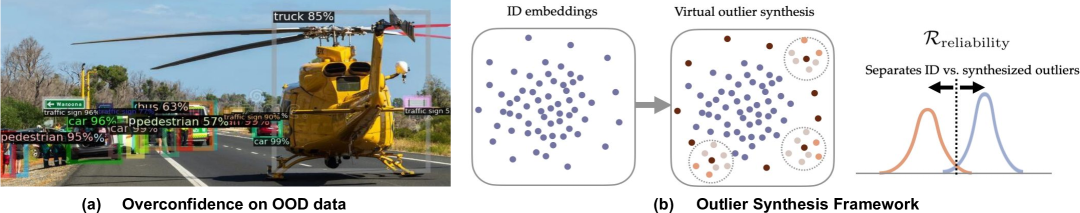
Figure 1: (a) An object detection model trained on BDD-100k dataset (DBLP:conf/cvpr/YuCWXCLMD20) produces overconfident predictions for OOD objects (e.g., helicopter), highlighting reliability concerns in ML models during deployment. Test images are sampled from MS-COCO (lin2014microsoft). (b) Overview of my proposed outlier synthesis framework for unknown-aware learning.

Reliable ML introduces core challenges in characterizing the reliability of off-the-shelf learning algorithms, which typically minimize errors on in-distribution (ID) data from $\mathbb{P}_{\text{in}}$ without accounting for uncertainties that could arise outside $\mathbb{P}_{\text{in}}$. For instance, the widely used empirical risk minimization (ERM) (vapnik1999nature), operates under the closed-world assumption (i.e., no distribution shift between training and inference). Models optimized with ERM are known to produce overconfidence predictions on OOD data (nguyen2015deep), since the decision boundary is not conservative. To address this challenge, my PhD research developed novel frameworks that jointly optimize for both: (1) accurate prediction of samples from $\mathbb{P}_{\text{in}}$, and (2) reliable handling of data from outside $\mathbb{P}_{\text{in}}$. Given a weighting factor $\alpha$, this can be formalized as follows:

$$\text{argmin}~~[\mathcal{R}_{\text{accuracy}}+~\alpha\cdot\mathcal{R}_{\text{reliability}}].\vskip-8.00003pt$$ (1)

As an example, $\mathcal{R}_{\text{accuracy}}$ can be the risk that classifies ID samples into known classes while $\mathcal{R}_{\text{reliability}}$ aims to distinguish ID vs. OOD. The introduction of the reliability risk term $\mathcal{R}_{\text{reliability}}$ is crucial to prevent overconfident predictions on unknown data and improve test-time reliability when encountering unknowns. However, incorporating this reliability risk requires large-scale human annotations, e.g., binary ID and OOD labels, which could limit the practical usage of the proposed framework. Therefore, my research contributes to developing the foundations of reliable machine learning with minimal human supervision, which spans three key aspects:

1. I developed novel unknown-aware learning frameworks that teach the models what they don’t know without having explicit knowledge about unknowns (Figure 1 (b)). The framework enables tractable learning from the unknowns by adaptively generating virtual outliers from the low-likelihood region in both the feature (Du et al., 2022c, b; tao2023nonparametric) and input space (Du et al., 2023), and shows strong efficacy and interpretability for regularizing the model to discriminate the boundaries between known and unknown data.

2. I designed algorithms and theoretical analysis for unknown-aware learning by leveraging unlabeled data collected from the models’ deployment environment. This wild data is a mixture of ID and OOD data by an unknown mixing ratio. Methods I designed such as gradient SVD score (Du et al., 2024a; Bai et al., 2024) and constrained optimization (Bai et al., 2023a) can facilitate OOD detection and generalization on these real-world reliability challenges.

3. I built reliable foundation models by investigating the reliability blind spots of language models, such as untruthful generations (Du et al., 2024d), malicious prompts (Du et al., 2024b), and noisy alignment data (yeh2024reliable). My work seeks to fundamentally understand the sources of these issues by developing algorithms that leverage unlabeled data to identify and mitigate the unintended information, which ensures safer human-AI interactions.

My thesis research has led to impactful publications in top-tier ML and vision venues and has been recognized by Rising Stars in Data Science and Jane Street Graduate Research Fellowship programs. Many of my works has been integrated into the OpenOOD benchmark (yang2022openood; zhang2023openood), and have received considerable follow-ups from worldwide major industry labs, such as Google (liu2023fast), Microsoft (narayanaswamy2023exploring), Amazon (Constantinou et al., 2024), Apple (zang2024overcoming), Adobe (Gu et al., 2023), Air Force Research (Inkawhich et al., 2024), Toyota (seifi2024ood), LG (yoon2024diffusion), Alibaba (lang2022estimating) etc. The scientific impact of reliable ML is profound, I am excited to explore interdisciplinary collaborations across computer science, statistics, biology science, and policy to push the boundaries of reliable ML as a machine learning researcher in the future.

The outline of this thesis is as follows: Chapter 2 states the background of the thesis research by introducing the problem setup, and reviewing the literature on out-of-distribution detection and reliable foundation models, which provide the broader conceptual framework for unknown-aware learning. Chapter 3 provides an overview of the first piece of my PhD research on foundations of unknown-aware learning. Chapters 4-6 present in order the three representative foundational works that (1) discuss the tractable learning foundation by outlier synthesis that is primarily based on the publications at ICLR’22 (Du et al., 2022c) and ICLR’23 (tao2023nonparametric); (2) introduce interpretable outlier synthesis to allow human-compatiable interpretation (Du et al., 2023); and (3) understand the impact of in-distribution data particularly on the effect of a compact representation space (Du et al., 2022a). Chapter 7 summarizes the contributions of the second piece of my PhD thesis research on learning in the wild with unlabeled data. Chapter 8 discusses algorithmic and theoretical advances in leveraging unlabeled wild data. We describe the proposed learning algorithm, optimization procedures, and generalization analyses. Chapter 9 contains the overview of the contributions for the final piece of my PhD thesis research on towards reliable foundation models. Chapter 10 expands the focus to large-scale language and multimodal models, examining issues of hallucination, and malicious user prompt attacks along with proposed solutions. Finally, Chapter 11 concludes the thesis, summarizing the key findings and envisioning how unknown-aware learning can further push the boundary of AI reliability.

Chapter 2 Background

In this chapter, we will first introduce the problem formulation in Section 1, and then discuss the related work to this thesis in Section 2.

1 Problem Formulation

1.1 Out-of-distribution Detection

The key idea in the unknown-aware learning framework is to perform OOD detection, which identifies data shifts, such as the data that belongs to semantic classes different from training, by performing thresholding on certain scoring functions. Formally, we describe the data setup, models and losses and learning goal.

Labeled ID data and ID distribution. Let $\mathcal{X}$ be the input space, and $\mathcal{Y}=\{1,...,K\}$ be the label space for ID data. Given an unknown ID joint distribution $\mathbb{P}_{\mathcal{X}\mathcal{Y}}$ defined over $\mathcal{X}\times\mathcal{Y}$, the labeled ID data $\mathcal{S}^{\text{in}}=\{(\mathbf{x}_{1},y_{1}),...,(\mathbf{x}_{n},y_{n})\}$ are drawn independently and identically from $\mathbb{P}_{\mathcal{X}\mathcal{Y}}$. We also denote $\mathbb{P}_{\text{in}}$ as the marginal distribution of $\mathbb{P}_{\mathcal{X}\mathcal{Y}}$ on $\mathcal{X}$, which is referred to as the ID distribution.

Out-of-distribution detection. Our framework concerns a common real-world scenario in which the algorithm is trained on the labeled ID data, but will then be deployed in environments containing OOD data from unknown class, i.e., $y\notin\mathcal{Y}$, and therefore should not be predicted by the model. At test time, the goal is to decide whether a test-time input is from ID or not (OOD).

Unlabeled wild data. A key challenge in OOD detection is the lack of labeled OOD data. In particular, the sample space for potential OOD data can be prohibitively large, making it expensive to collect labeled OOD data. In this thesis (particularly in Chapter 8), to model the realistic environment, we incorporate unlabeled wild data $\mathcal{S}_{\text{wild}}=\left\{\tilde{\mathbf{x}}_{1},...,\tilde{\mathbf{x}}_{m}\right\}$ into our learning framework. Wild data consists of both ID and OOD data, and can be collected freely upon deploying an existing model trained on $\mathcal{S}^{\text{in}}$. Following Katz-Samuels et al. (2022), we use the Huber contamination model to characterize the marginal distribution of the wild data

$$\mathbb{P}_{\text{wild}}:=(1-\pi)\mathbb{P}_{\text{in}}+\pi\mathbb{P}_{\text{out}},$$ (2)

where $\pi\in(0,1]$ and $\mathbb{P}_{\text{out}}$ is the OOD distribution defined over $\mathcal{X}$. Note that the case $\pi=0$ is straightforward since no novelties occur.

Models and losses. We denote by $\mathbf{h}_{\mathbf{w}}:\mathcal{X}\mapsto\mathbb{R}^{K}$ a predictor for ID classification with parameter $\mathbf{w}\in\mathcal{W}$, where $\mathcal{W}$ is the parameter space. $\mathbf{h}_{\mathbf{w}}$ returns the soft classification output. We consider the loss function $\ell:\mathbb{R}^{K}\times\mathcal{Y}\mapsto\mathbb{R}$ on the labeled ID data. In addition, we denote the OOD classifier $\mathbf{g}_{\boldsymbol{\theta}}:\mathcal{X}\mapsto\mathbb{R}$ with parameter ${\boldsymbol{\theta}}\in\Theta$, where $\Theta$ is the parameter space. We use $\ell_{\text{b}}(\mathbf{g}_{\boldsymbol{\theta}}(\mathbf{x}),y_{\text{b}})$ to denote the binary loss function w.r.t. $\mathbf{g}_{\boldsymbol{\theta}}$ and binary label $y_{\text{b}}\in\mathcal{Y}_{\text{b}}:=\{y_{+},y_{-}\}$, where $y_{+}\in\mathbb{R}_{>0}$ and $y_{-}\in\mathbb{R}_{<0}$ correspond to the ID class and the OOD class, respectively.

Learning goal. Our learning framework aims to build the OOD classifier $\mathbf{g}_{\boldsymbol{\theta}}$ by leveraging data from either $\mathcal{S}^{\text{in}}$ only (Chapters 3-6) or the joint set of $\mathcal{S}^{\text{in}}$ and $\mathcal{S}_{\text{wild}}$ (Chapter 8). In evaluating our model, we are interested in the following measurements:

$$(1)~\downarrow\text{FPR}(\mathbf{g}_{\boldsymbol{\theta}};\lambda)=\mathbb{E}_{\mathbf{x}\sim\mathbb{P}_{\text{out}}}(\mathds{1}{\{\mathbf{g}_{\boldsymbol{\theta}}(\mathbf{x})>\lambda\}}),$$ (3)

$$(2)~\uparrow\text{TPR}(\mathbf{g}_{\boldsymbol{\theta}};\lambda)=\mathbb{E}_{\mathbf{x}\sim\mathbb{P}_{\text{in}}}(\mathds{1}{\{\mathbf{g}_{\boldsymbol{\theta}}(\mathbf{x})>\lambda\}}),$$

where $\lambda$ is a threshold, typically chosen so that a high fraction of ID data is correctly classified. In Chapters 4 and 6, we include the object-level OOD detection task during evaluation, where we will discuss the problem setup more concretely there.

1.2 Hallucination Detection

The third piece of this PhD thesis focuses on LLM safety (Chapter 10), specifically on LLM hallucination detection with a safety emphasis on the model outputs compared to OOD detection. Formally, we describe the LLM generation and the problem of hallucination detection.

LLM generation. We consider an $L$-layer causal LLM, which takes a sequence of $n$ tokens $\mathbf{x}_{\text{prompt}}=\{x_{1},...,x_{n}\}$, and generates an output $\mathbf{x}_{o}=\{x_{n+1},...,x_{n+m}\}$ in an autoregressive manner. Each output token $x_{i},i\in[n+1,...,n+m]$ is sampled from a distribution over the model vocabulary $\mathcal{V}$, conditioned on the prefix $\{x_{1},...,x_{i-1}\}$:

$$x_{i}=\operatorname{argmax}_{x\in\mathcal{V}}P(x|\{x_{1},...,x_{i-1}\}),$$ (4)

and the probability $P$ is calculated as:

$$P(x|\{x_{1},...,x_{i-1}\})=\operatorname{softmax}(\mathbf{w}_{o}\mathbf{f}_{L}(x)+\mathbf{b}_{o}),$$ (5)

where $\mathbf{f}_{L}(x)\in\mathbb{R}^{d}$ denotes the representation at the $L$-th layer of LLM for token $x$, and $\mathbf{w}_{o},\mathbf{b}_{o}$ are the weight and bias parameters at the final output layer.

Hallucination detection. We denote $\mathbb{P}_{\text{true}}$ as the joint distribution over the truthful input and generation pairs, which is referred to as truthful distribution. For any given generated text $\mathbf{x}_{o}$ and its corresponding input prompt $\mathbf{x}_{\text{prompt}}$ where $(\mathbf{x}_{\text{prompt}},\mathbf{x}_{o})\in\mathcal{X}_{LLM}$, the goal of hallucination detection is to learn a binary predictor $G:\mathcal{X}_{LLM}\rightarrow\{0,1\}$ such that

$$G({\color[rgb]{0,0,0}\mathbf{x}_{\text{prompt}},\mathbf{x}_{o}})=\begin{cases}\;1,\hskip 11.38109pt&\text{if }\;{\color[rgb]{0,0,0}(\mathbf{x}_{\text{prompt}},\mathbf{x}_{o})}\sim\mathbb{P}_{\text{true}}\\ \;0,&\text{otherwise}\end{cases}$$ (6)

2 Related Work

This section includes an introduction to related work in out-of-distribution detection and LLM hallucination detection, which touches both the algorithmic and theoretical research results. Additionally, each chapter includes discussions on other research areas relevant to its specific topic.

2.1 Literature on OOD Detection

OOD detection has attracted a surge of interest in recent years (Fort et al., 2021; yang2021generalized; Fang et al., 2022; zhu2022boosting; ming2022delving; ming2022spurious; yang2022openood; wang2022outofdistribution; Galil et al., 2023; Djurisic et al., 2023; zheng2023out; wang2022watermarking; wang2023outofdistribution; narasimhan2023learning; yang2023auto; uppaal2023fine; zhu2023diversified; zhu2023unleashing; ming2023finetune; zhang2023openood; Ghosal et al., 2024). One line of work performs OOD detection by devising scoring functions, including confidence-based methods (Bendale and Boult, 2016; Hendrycks and Gimpel, 2017; liang2018enhancing), energy-based score (liu2020energy; wang2021canmulti; wu2023energybased), distance-based approaches (lee2018simple; tack2020csi; DBLP:journals/corr/abs-2106-09022; 2021ssd; sun2022out; Du et al., 2022a; ming2023cider; ren2023outofdistribution), gradient-based score (Huang et al., 2021), and Bayesian approaches (Gal and Ghahramani, 2016; lakshminarayanan2017simple; maddox2019simple; dpn19nips; Wen2020BatchEnsemble; Kristiadi et al., 2020). Another line of work addressed OOD detection by training-time regularization (Bevandić et al., 2018; malinin2018predictive; Geifman and El-Yaniv, 2019; Hein et al., 2019; meinke2019towards; Jeong and Kim, 2020; liu2020simple; van Amersfoort et al., 2020; DBLP:conf/iccv/YangWFYZZ021; DBLP:conf/icml/WeiXCF0L22; Du et al., 2022b, 2023; wang2023learning). For example, the model is regularized to produce lower confidence (lee2018training) or higher energy (liu2020energy; Du et al., 2022c) on a set of clean OOD data (Hendrycks et al., 2019; DBLP:conf/icml/MingFL22), wild data (zhou2021step; Katz-Samuels et al., 2022; He et al., 2023; Bai et al., 2023a; Du et al., 2024a) and synthetic outliers (Du et al., 2023; tao2023nonparametric; park2023powerfulness).

OOD detection for object detection is a rising topic with very few existing works. For Faster R-CNN, My work VOS (Du et al., 2022c) proposed to synthesize virtual outliers in the feature space for model regularization. Du et al. (2022b) explored unknown-aware object detection by leveraging videos in the wild, whereas we focus on settings with still images only. For transformer-based object detection model detr, Gupta et al. (2022) adopted unmatched object queries that are with high confidence as unknowns, which did not focus on regularizing the model for desirable representations. Several works (Deepshikha et al., 2021; Dhamija et al., 2020; Hall et al., 2020; DBLP:conf/icra/MillerDMS19; DBLP:conf/icra/MillerNDS18) used approximate Bayesian methods, such as MC-Dropout (Gal and Ghahramani, 2016) for OOD detection. They require multiple inference passes to generate the uncertainty score, which are computationally expensive on larger datasets and models.

2.2 Literature on OOD Detection Theory

Recent studies have begun to focus on the theoretical understanding of OOD detection.  Fang et al. (2022) studied the generalization of OOD detection by PAC learning and they found a necessary condition for the learnability of OOD detection. morteza2022provable derived a novel OOD score and provided a provable understanding of the OOD detection result using that score. My work at ICLR’24 (Du et al., 2024a) theoretically studied the impact of unlabeled data for OOD detection. Later at ICML’24, my work (Du et al., 2024c) formally analyzed the impact of ID labels on OOD detection, which has not been studied in the past.

2.3 Literature on Hallucination Detection

Hallucination detection has gained interest recently for ensuring LLMs’ safety and reliability (Guerreiro et al., 2022; Huang et al., 2023a; Ji et al., 2023; zhang2023siren; xu2024hallucination; zhang2023enhancing; Chern et al., 2023; min2023factscore; Huang et al., 2023b; ren2023outofdistribution; wang2023hallucination). The majority of work performs hallucination detection by devising uncertainty scoring functions, including those based on the logits (Andrey and Mark, 2021; kuhn2023semantic; Duan et al., 2023) that assumed hallucinations would be generated by flat token log probabilities, and methods that are based on the output texts, which either measured the consistency of multiple generated texts  (manakul2023selfcheckgpt; Agrawal et al., 2024; mundler2023self; xiong2023can; Cohen et al., 2023) or prompted LLMs to evaluate the confidence on their generations (Kadavath et al., 2022; xiong2023can; ren2023self; lin2022teaching; tian2023just; zhou2023navigating). Additionally, there is growing interest in exploring the LLM activations to determine whether an LLM generation is true or false (su2024unsupervised; yin2024characterizing; rateike2023weakly). For example,  Chen et al. (2024) performed eigendecomposition with activations but the decomposition was done on the covariance matrix that required multiple generation steps to measure the consistency. zou2023representation explored probing meaningful direction from neural activations. Another branch of works, such as (li2023inference; Duan et al., 2024; Azaria and Mitchell, 2023), employed labeled data for extracting truthful directions, which differs from the scope on harnessing unlabeled LLM generations that is explored in this thesis. Note that our studied problem is different from the research on hallucination mitigation (lee2022factuality; tian2019sticking; zhang2023alleviating; Kai et al., 2024; shi2023trusting; Chuang et al., 2024), which aims to enhance the truthfulness of LLMs’ decoding process. Some of my thesis works, such as (Bai et al., 2024; Du et al., 2024a; Bai et al., 2023a) can be closely connected with hallucination detection with unlabeled LLM generations, which utilized unlabeled data for out-of-distribution detection. However, their approach and problem formulation are different.

Chapter 3 Overview for Foundations of Unknown-Aware Learning

Motivation. Ensuring safe and reliable AI systems requires addressing a critical issue: the overconfident predictions made on the OOD inputs (nguyen2015deep). These inputs arise from unknown categories and should ideally be excluded from model predictions. For example, in self-driving car applications, my research is the first to discover that an object detection model trained on ID objects (e.g., cars, pedestrians) might confidently misidentify an unusual object, such as a helicopter on a highway, as a known object; see Figure 1 (a). Such failures not only raise concerns about model reliability but also pose serious risks in safety-critical deployments.

The vulnerability to OOD inputs stems from the lack of explicit knowledge of unknowns during training, as neural networks are typically optimized only on ID data. While this approach effectively captures ID tasks, the resulting decision boundaries can be inadequate for OOD detection. Ideally, a model should maintain high confidence for ID data and exhibit high uncertainty for OOD samples, yet achieving this goal is challenging due to the absence of labeled outliers. My research tackles this challenge for unknown-aware learning through an automated outlier generation paradigm, which offers greater feasibility and flexibility than approaches requiring extensive human annotations (Hendrycks et al., 2019). I outline three core fundamental contributions between Chapter 4 and Chapter 6:

Tractable learning foundation by outlier synthesis. My work VOS (Du et al., 2022c) (ICLR’22) laid the foundation of a learning framework called virtual outlier synthesis to regularize the models’ decision boundary. This approach is based on modeling ID features as Gaussians, reject sampling to synthesize virtual outliers from low-likelihood regions, and a novel unknown-aware training objective that contrastively shapes the uncertainty energy surface between ID data and synthesized outliers. Additionally, VOS delivers the insight that synthesizing outliers in the feature space is more tractable than generating high-dimensional pixels (lee2018training). My subsequent work, NPOS (tao2023nonparametric) (ICLR’23), relaxed the Gaussian assumption through a non-parametric synthesis approach, yielding improved results on language models and larger datasets. The STUD method (Du et al., 2022b), presented at CVPR’22 as an oral, further demonstrated the efficacy of this approach in real-world practice, i.e., video object detection, distilling unknown objects in both spatial and temporal dimensions to regularize model decision boundaries. Particularly, Chapter 4 is going to mainly discuss the work of VOS.

Interpretable outlier synthesis. While feature-space synthesis is effective, it doesn’t allow human-compatible interpretation like visual pixels. To address this, my NeurIPS’23 paper Dream-OOD (Du et al., 2023) introduced a framework to comprehensively study the interactions between feature-space and pixel-space synthesis. The method learns a text-conditioned visual latent space, enabling outlier sampling and decoding by diffusion models, which not only enhances interpretability but also achieves strong results on OOD detection benchmarks. It has garnered quite a few interests from community, prompting follow-up research on pixel-space outlier synthesis (yoon2024diffusion; um2024self; liu2024can). Chapter 5 will cover the work of Dream-OOD.

Understanding the impact of in-distribution data. Beyond focusing on reliability risks in the unknown-aware learning framework, it’s crucial to address the in-distribution accuracy term $\mathcal{R}_{\text{accuracy}}$ in Equation 1 during training. My work, SIREN (Du et al., 2022a) (NeurIPS’22) and a subsequent ICML’24 paper (Du et al., 2024c), fundamentally investigated the influence of compact representation space and ID label supervision on identifying OOD samples. These insights contribute to designing better training strategies on ID data and enhancing overall model reliability. In Chapter 6, we will focus on the work of SIREN.

Chapter 4 VOS: Learning What You Don’t Know by Virtual Outlier Synthesis

Publication Statement. This chapter is joint work with Zhaoning Wang, Mu Cai and Yixuan Li. The paper version of this chapter appeared in ICLR’22 (Du et al., 2022c).

Abstract. OOD detection has received much attention lately due to its importance in the safe deployment of neural networks. One of the key challenges is that models lack supervision signals from unknown data, and as a result, can produce overconfident predictions on OOD data. Previous approaches rely on real outlier datasets for model regularization, which can be costly and sometimes infeasible to obtain in practice. In this chapter, we present VOS, a novel framework for OOD detection by adaptively synthesizing virtual outliers that can meaningfully regularize the model’s decision boundary during training. Specifically, VOS samples virtual outliers from the low-likelihood region of the class-conditional distribution estimated in the feature space. Alongside, we introduce a novel unknown-aware training objective, which contrastively shapes the uncertainty space between the ID data and synthesized outlier data. VOS achieves competitive performance on both object detection and image classification models, reducing the FPR95 by up to 9.36% compared to the previous best method on object detectors. Code is available at https://github.com/deeplearning-wisc/vos.

3 Introduction

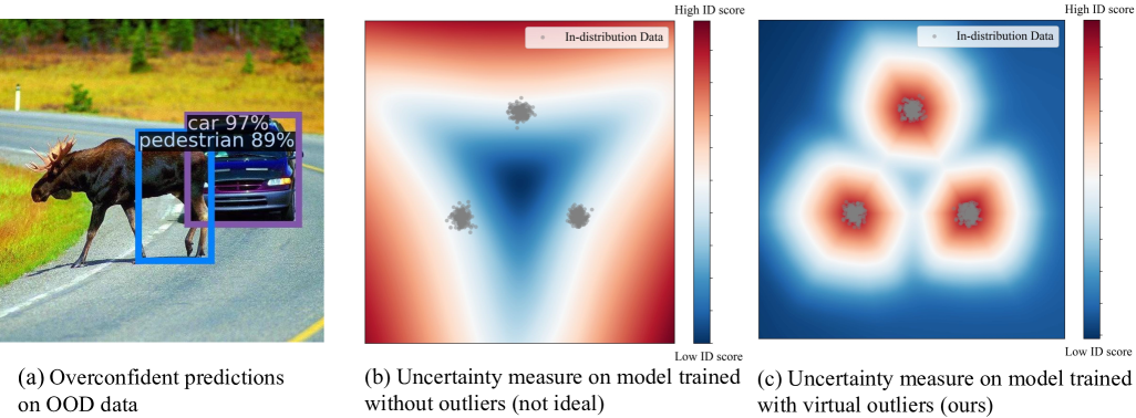
Figure 2: (a) A Faster-RCNN (ren2015faster) model trained on BDD-100k dataset (DBLP:conf/cvpr/YuCWXCLMD20) produces overconfident predictions for OOD object (e.g., moose). (b)-(c) The uncertainty measurement with and without virtual outlier training. The in-distribution data $\mathbf{x}\in\mathcal{X}=\mathbb{R}^{2}$ is sampled from a Gaussian mixture model). Regularizing the model with virtual outliers (c) better captures the OOD uncertainty than without (b).

Modern deep neural networks have achieved unprecedented success in known contexts for which they are trained, yet they often struggle to handle the unknowns. In particular, neural networks have been shown to produce high posterior probability for out-of-distribution (OOD) test inputs (nguyen2015deep), which arise from unknown categories and should not be predicted by the model. Taking self-driving car as an example, an object detection model trained to recognize in-distribution objects (e.g., cars, stop signs) can produce a high-confidence prediction for an unseen object of a moose; see Figure 2(a). Such a failure case raises concerns in model reliability, and worse, may lead to catastrophe when deployed in safety-critical applications.

The vulnerability to OOD inputs arises due to the lack explicit knowledge of unknowns during training time. In particular, neural networks are typically optimized only on the in-distribution (ID) data. The resulting decision boundary, despite being useful on ID tasks such as classification, can be ill-fated for OOD detection. We illustrate this in Figure 2. The ID data (gray) consists of three class-conditional Gaussians, on which a three-way softmax classifier is trained. The resulting classifier is overconfident for regions far away from the ID data (see the red shade in Figure 2(b)), causing trouble for OOD detection. Ideally, a model should learn a more compact decision boundary that produces low uncertainty for the ID data, with high OOD uncertainty elsewhere (e.g., Figure 2(c)). However, achieving this goal is non-trivial due to the lack of supervision signal of unknowns. This motivates the question: Can we synthesize virtual outliers for effective model regularization?

In this chapter, we propose a novel unknown-aware learning framework dubbed VOS (Virtual Outlier Synthesis), which optimizes the dual objectives of both ID task and OOD detection performance. In a nutshell, VOS consists of three components tackling challenges of outlier synthesis and effective model regularization with synthesized outliers. To synthesize the outliers, we estimate the class-conditional distribution in the feature space, and sample outliers from the low-likelihood region of ID classes (Section 5.1). Key to our method, we show that sampling in the feature space is more tractable than synthesizing images in the high-dimensional pixel space (lee2018training). Alongside, we propose a novel unknown-aware training objective, which contrastively shapes the uncertainty surface between the ID data and synthesized outliers (Section 5.2). During training, VOS simultaneously performs the ID task (e.g., classification or object detection) as well as the OOD uncertainty regularization. During inference time, the uncertainty estimation branch produces a larger probabilistic score for ID data and vice versa, which enables effective OOD detection (Section 5.3).

VOS offers several compelling advantages compared to existing solutions. (1) VOS is a general learning framework that is effective for both object detection and image classification tasks, whereas previous methods were primarily driven by image classification. Image-level detection can be limiting as an image could be OOD in certain regions while being in-distribution elsewhere. Our work bridges a critical research gap since OOD detection for object detection is timely yet underexplored in literature. (2) VOS enables adaptive outlier synthesis, which can be flexibly and conveniently used for any ID data without manual data collection or cleaning. In contrast, previous methods using outlier exposure (Hendrycks et al., 2019) require an auxiliary image dataset that is sufficiently diverse, which can be arguably prohibitive to obtain. Moreover, one needs to perform careful data cleaning to ensure the auxiliary outlier dataset does not overlap with ID data. (3) VOS synthesizes outliers that can estimate a compact decision boundary between ID and OOD data. In contrast, existing solutions use outliers that are either too trivial to regularize the OOD estimator, or too hard to be separated from ID data, resulting in sub-optimal performance.

Our key contributions and results are summarized as follows:

• We propose a new framework VOS addressing a pressing issue—unknown-aware deep learning that optimizes for both ID and OOD performance. VOS establishes state-of-the-art results on a challenging object detection task. Compared to the best method, VOS reduces the FPR95 by up to 9.36% while preserving the accuracy on the ID task.

• We conduct extensive ablations and reveal important insights by contrasting different outlier synthesis approaches. We show that VOS is more advantageous than generating outliers directly in the high-dimensional pixel space (e.g., using GAN (lee2018training)) or using noise as outliers.

• We comprehensively evaluate our method on common OOD detection benchmarks, along with a more challenging yet underexplored task in the context of object detection. Our effort facilitates future research to evaluate OOD detection in a real-world setting.

4 Problem Setup

We start by formulating the problem of OOD detection in the setting of object detection. Our framework can be easily generalized to image classification when the bounding box is the entire image (see Section 6.2). Most previous formulations of OOD detection treat entire images as anomalies, which can lead to ambiguity shown in Figure 2. In particular, natural images are composed of numerous objects and components. Knowing which regions of an image are anomalous could allow for safer handling of unfamiliar objects. This setting is more realistic in practice, yet also more challenging as it requires reasoning OOD uncertainty at the fine-grained object level.

Specifically, we denote the input and label space by $\mathcal{X}=\mathbb{R}^{d}$ and $\mathcal{Y}=\{1,2,...,K\}$, respectively. Let $\mathbf{x}\in\mathcal{X}$ be the input image, $\mathbf{b}\in\mathbb{R}^{4}$ be the bounding box coordinates associated with object instances in the image, and $y\in\mathcal{Y}$ be the semantic label for $K$-way classification. An object detection model is trained on in-distribution data $\mathcal{D}=\left\{\left(\mathbf{x}_{i},\mathbf{b}_{i},{y}_{i}\right)\right\}_{i=1}^{N}$ drawn from an unknown joint distribution $mathcal{P}$. We use neural networks with parameters $\theta$ to model the bounding box regression $p_{\theta}(\mathbf{b}|\mathbf{x})$ and the classification $p_{\theta}(y|\mathbf{x},\mathbf{b})$.

The OOD detection can be formulated as a binary classification problem, which distinguishes between the in- vs. out-of-distribution objects. Let $P_{\mathcal{X}}$ denote the marginal probability distribution on $\mathcal{X}$. Given a test input $\mathbf{x}^{*}\sim P_{\mathcal{X}}$, as well as an object instance $\mathbf{b}^{*}$ predicted by the object detector, the goal is to predict $p_{\theta}(g|\mathbf{x}^{*},\mathbf{b}^{*})$. We use $g=1$ to indicate a detected object being in-distribution, and $g=0$ being out-of-distribution, with semantics outside the support of $\mathcal{Y}$.

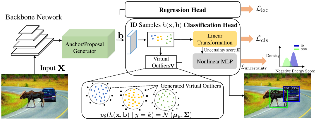
Figure 3: The framework of VOS. We model the feature representation of ID objects as class-conditional Gaussians, and sample virtual outliers $\mathbf{v}$ from the low-likelihood region. The virtual outliers, along with the ID objects, are used to produce the uncertainty loss for regularization. The uncertainty estimation branch ($\mathcal{L}_{\mathrm{uncertainty}}$) is jointly trained with the object detection loss ($\mathcal{L}_{\mathrm{loc}},\mathcal{L}_{\mathrm{cls}}$).

5 Method

Our novel unknown-aware learning framework is illustrated in Figure 3. Our framework encompasses three novel components and addresses the following questions: (1) how to synthesize the virtual outliers (Section 5.1), (2) how to leverage the synthesized outliers for effective model regularization (Section 5.2), and (3) how to perform OOD detection during inference time (Section 5.3)?

5.1 VOS: Virtual Outlier Synthesis

Our framework VOS generates virtual outliers for model regularization, without relying on external data. While a straightforward idea is to train generative models such as GANs (Goodfellow et al., 2014; lee2018training), synthesizing images in the high-dimensional pixel space can be difficult to optimize. Instead, our key idea is to synthesize virtual outliers in the feature space, which is more tractable given lower dimensionality. Moreover, our method is based on a discriminatively trained classifier in the object detector, which circumvents the difficult optimization process in training generative models.

Specifically, we assume the feature representation of object instances forms a class-conditional multivariate Gaussian distribution (see Figure 4):

$$p_{\theta}(h(\mathbf{x},\mathbf{b})|y=k)=\mathcal{N}(\boldsymbol{\mu}_{k},\boldsymbol{\Sigma}),$$

where $\boldsymbol{\mu}_{k}$ is the Gaussian mean of class $k\in\{1,2,..,\mathrm{K}\}$, $\boldsymbol{\Sigma}$ is the tied covariance matrix, and $h(\mathbf{x},\mathbf{b})\in\mathbb{R}^{m}$ is the latent representation of an object instance $(\mathbf{x},\mathbf{b})$. To extract the latent representation, we use the penultimate layer of the neural network. The dimensionality $m$ is significantly smaller than the input dimension $d$.

Figure 4: UMAP visualization of feature embeddings of PASCAL-VOC (on a subset of 10 classes).

To estimate the parameters of the class-conditional Gaussian, we compute empirical class mean $\widehat{\boldsymbol{\mu}}_{k}$ and covariance $\widehat{\boldsymbol{\Sigma}}$ of training samples $\left\{\left(\mathbf{x}_{i},\mathbf{b}_{i},{y}_{i}\right)\right\}_{i=1}^{N}$:

$$\widehat{\boldsymbol{\mu}}_{k} =\frac{1}{N_{k}}\sum_{i:y_{i}=k}h(\mathbf{x}_{i},\mathbf{b}_{i})$$ (7)

$$\widehat{\boldsymbol{\Sigma}} =\frac{1}{N}\sum_{k}\sum_{i:y_{i}=k}\left(h(\mathbf{x}_{i},\mathbf{b}_{i})-\widehat{\boldsymbol{\mu}}_{k}\right)\left(h(\mathbf{x}_{i},\mathbf{b}_{i})-\widehat{\boldsymbol{\mu}}_{k}\right)^{\top},$$ (8)

where $N_{k}$ is the number of objects in class $k$, and $N$ is the total number of objects. We use online estimation for efficient training, where we maintain a class-conditional queue with $|Q_{k}|$ object instances from each class. In each iteration, we enqueue the embeddings of objects to their corresponding class-conditional queues, and dequeue the same number of object embeddings.

Sampling from the feature representation space. We propose sampling the virtual outliers from the feature representation space, using the multivariate distributions estimated above. Ideally, these virtual outliers should help estimate a more compact decision boundary between ID and OOD data.

To achieve this, we propose sampling the virtual outliers $\mathcal{V}_{k}$ from the $\epsilon$-likelihood region of the estimated class-conditional distribution:

$$\mathcal{V}_{k}=\{\mathbf{v}_{k} |\frac{1}{(2\pi)^{m/2}|\widehat{\mathbf{\boldsymbol{\Sigma}}}|^{1/2}}\exp\left(-\frac{1}{2}(\mathbf{v}_{k}-\widehat{\boldsymbol{\mu}}_{k})^{\top}\widehat{\boldsymbol{\Sigma}}^{-1}(\mathbf{v}_{k}-\widehat{\boldsymbol{\mu}}_{k})\right)<\epsilon\},$$ (9)

where $\mathbf{v}_{k}\sim\mathcal{N}(\widehat{\boldsymbol{\mu}}_{k},\widehat{\boldsymbol{\Sigma}})$ denotes the sampled virtual outliers for class $k$, which are in the sublevel set based on the likelihood. $\epsilon$ is sufficiently small so that the sampled outliers are near class boundary.

Classification outputs for virtual outliers. For a given sampled virtual outlier $\mathbf{v}\in\mathbb{R}^{m}$, the output of the classification branch can be derived through a linear transformation:

$$f(\mathbf{v};\theta)=W_{\text{cls}}^{\top}\mathbf{v},$$ (10)

where $W_{\text{cls}}\in\mathbb{R}^{m\times K}$ is the weight of the last fully connected layer. We proceed with describing how to regularize the output of virtual outliers for improved OOD detection.

5.2 Unknown-aware Training Objective

We now introduce a new training objective for unknown-aware learning, leveraging the virtual outliers in Section 5.1. The key idea is to perform visual recognition task while regularizing the model to produce a low OOD score for ID data, and a high OOD score for the synthesized outlier.

Uncertainty regularization for classification.

For simplicity, we first describe the regularization in the multi-class classification setting. The regularization loss should ideally optimize for the separability between the ID vs. OOD data under some function that captures the data density. However, directly estimating $\log p(\mathbf{x})$ can be computationally intractable as it requires sampling from the entire space $\mathcal{X}$. We note that the log partition function $E(\mathbf{x};\theta):=-\log\sum_{k=1}^{K}e^{f_{k}(\mathbf{x};\theta)}$ is proportional to $\log p(\mathbf{x})$ with some unknown factor, which can be seen from the following:

$$p(y|\mathbf{x})=\frac{p(\mathbf{x},y)}{p(\mathbf{x})}=\frac{e^{f_{y}(\mathbf{x};\theta)}}{\sum_{k=1}^{K}e^{f_{k}(\mathbf{x};\theta)}},$$

where $f_{y}(\mathbf{x};{\theta})$ denotes the $y$-th element of logit output corresponding to the label $y$. The negative log partition function is also known as the free energy, which was shown to be an effective uncertainty measurement for OOD detection (liu2020energy).

Our idea is to explicitly perform a level-set estimation based on the energy function (threshold at 0), where the ID data has negative energy values and the synthesized outlier has positive energy:

$$\mathcal{L}_{\text{uncertainty}}=\mathbb{E}_{\mathbf{v}\sim\mathcal{V}}~~\mathds{1}\{E(\mathbf{v};\theta)>0\}+\mathbb{E}_{\mathbf{x}\sim\mathcal{D}}~~\mathds{1}\{E(\mathbf{x};\theta)\leq 0\}$$

This is a simpler objective than estimating density. Since the $0/1$ loss is intractable, we replace it with the binary sigmoid loss, a smooth approximation of the $0/1$ loss, yielding the following:

$$\mathcal{L}_{\text{uncertainty}}=\mathbb{E}_{\mathbf{v}\sim\mathcal{V}}\left[-\log\frac{1}{1+\exp^{-\phi(E(\mathbf{v};\theta))}}\right]+\mathbb{E}_{{\mathbf{x}\sim\mathcal{D}}}\left[-\log\frac{\exp^{-\phi(E(\mathbf{x};\theta))}}{1+\exp^{-\phi(E(\mathbf{x};\theta))}}\right].$$ (11)

Here $\phi(\cdot)$ is a nonlinear MLP function, which allows learning flexible energy surface. The learning process shapes the uncertainty surface, which predicts high probability for ID data and low probability for virtual outliers $\mathbf{v}$.  liu2020energy employed energy for model uncertainty regularization, however, the loss function is based on the squared hinge loss and requires tuning two margin hyperparameters. In contrast, our uncertainty regularization loss is completely hyperparameter-free and is much easier to use in practice. Moreover, VOS produces probabilistic score for OOD detection, whereas liu2020energy relies on non-probabilistic energy score.

Object-level energy score.

In case of object detection, we can replace the image-level energy with object-level energy score. For ID object $(\mathbf{x},\mathbf{b})$, the energy is defined as:

$$E(\mathbf{x},\mathbf{b};\theta)=-\log\sum_{k=1}^{K}w_{k}\cdot\exp^{f_{k}((\mathbf{x},\mathbf{b});\theta)},\vskip-3.99994pt$$ (12)

where $f_{k}((\mathbf{x},\mathbf{b});\theta)=W^{\top}_{\text{cls}}h(\mathbf{x},\mathbf{b})$ is the logit output for class $k$ in the classification branch. The energy score for the virtual outlier can be defined in a similar way as above. In particular, we will show in Section 6 that a learnable $\mathbf{w}$ is more flexible than a constant $\mathbf{w}$, given the inherent class imbalance in object detection datasets. Additional analysis on $w_{k}$ is in Appendix 30.7.

Overall training objective.

In the case of object detection, the overall training objective combines the standard object detection loss, along with a regularization loss in terms of uncertainty:

$$\min_{\theta}\mathbb{E}_{(\mathbf{x},\mathbf{b},{y})\sim\mathcal{D}}~~\left[\mathcal{L}_{\text{cls}}+\mathcal{L}_{\text{loc}}\right]+\beta\cdot\mathcal{L}_{\text{uncertainty}},$$ (13)

where $\beta$ is the weight of the uncertainty regularization. $\mathcal{L}_{\text{cls}}$ and $\mathcal{L}_{\text{loc}}$ are losses for classification and bounding box regression, respectively. This can be simplified to classification task without $\mathcal{L}_{\text{loc}}$. We provide ablation studies in Section 6.1 demonstrating the superiority of our loss function.

Input: ID data $\mathcal{D}=\left\{\left(\mathbf{x}_{i},\mathbf{b}_{i},{y}_{i}\right)\right\}_{i=1}^{N}$, randomly initialized detector with parameter $\theta$, queue size $|Q_{k}|$ for Gaussian density estimation, weight for uncertainty regularization $\beta$, and $\epsilon$.

Output: Object detector with parameter $\theta^{*}$, and OOD detector $G$.

while train do

    Update the ID queue $Q_{k}$ with the training objects $\{(\mathbf{x},{\mathbf{b}},y)\}$.;

   

   Estimate the multivariate distributions based on ID training objects using Equation 1 and 8.;

   

   Sample virtual outliers $\mathbf{v}$ using Equation 9.

   Calculate the regularization loss using Equation 11, update the parameters $\theta$ based on Equation 13.

end while

while eval do

    Calculate the OOD uncertainty score using Equation 14.;

   

   Perform thresholding comparison using Equation 15.

end while

Algorithm 1 VOS: Virtual Outlier Synthesis for OOD detection

5.3 Inference-time OOD Detection

During inference, we use the output of the logistic regression uncertainty branch for OOD detection. In particular, given a test input $\mathbf{x}^{*}$, the object detector produces a bounding box prediction $\mathbf{b}^{*}$. The OOD uncertainty score for the predicted object $(\mathbf{x}^{*},\mathbf{b}^{*})$ is given by:

$$p_{\theta}(g\mid\mathbf{x}^{*},\mathbf{b}^{*})=\frac{\exp^{-\phi(E(\mathbf{x}^{*},\mathbf{b}^{*}))}}{1+\exp^{-\phi(E(\mathbf{x}^{*},\mathbf{b}^{*}))}}.\vskip-5.0pt$$ (14)

For OOD detection, one can exercise the thresholding mechanism to distinguish between ID and OOD objects:

$$G(\mathbf{x}^{*},\mathbf{b}^{*})=\left\{\begin{array}[]{ll}1&\text{ if }p_{\theta}(g\mid\mathbf{x}^{*},\mathbf{b}^{*})\geq\gamma,\\ 0&\text{ if }p_{\theta}(g\mid\mathbf{x}^{*},\mathbf{b}^{*})<\gamma.\end{array}\right.$$ (15)

The threshold $\gamma$ is typically chosen so that a high fraction of ID data (e.g., 95%) is correctly classified. Our framework VOS is summarized in Algorithm 1.

6 Experimental Results

In this section, we present empirical evidence to validate the effectiveness of VOS on several real-world tasks, including both object detection (Section 6.1) and image classification (Section 6.2).

6.1 Evaluation on Object Detection

In-distribution $\mathcal{D}$	Method	FPR95 $\downarrow$	AUROC $\uparrow$	mAP (ID)$\uparrow$
		OOD: MS-COCO / OpenImages
PASCAL-VOC	MSP (Hendrycks and Gimpel, 2017)	70.99 / 73.13	83.45 / 81.91	48.7
	ODIN (liang2018enhancing)	59.82 / 63.14	82.20 / 82.59	48.7
	Mahalanobis (lee2018simple)	96.46 / 96.27	59.25 / 57.42	48.7
	Energy score (liu2020energy)	56.89 / 58.69	83.69 / 82.98	48.7
	Gram matrices (DBLP:conf/icml/SastryO20)	62.75 / 67.42	79.88 / 77.62	48.7
	Generalized ODIN (Hsu et al., 2020)	59.57 / 70.28	83.12 / 79.23	48.1
	CSI (tack2020csi)	59.91 / 57.41	81.83 / 82.95	48.1
	GAN-synthesis (lee2018training)	60.93 / 59.97	83.67 / 82.67	48.5
	VOS-ResNet50 (ours)	47.53$\pm$2.9 / 51.33$\pm$1.6	88.70$\pm$1.2 / 85.23$\pm$ 0.6	48.9$\pm$0.2
	VOS-RegX4.0 (ours)	47.77$\pm$1.1 / 48.33$\pm$1.6	89.00$\pm$0.4 / 87.59$\pm$0.2	51.6$\pm$0.1
Berkeley DeepDrive-100k	MSP (Hendrycks and Gimpel, 2017)	80.94 / 79.04	75.87 / 77.38	31.2
	ODIN (liang2018enhancing)	62.85 / 58.92	74.44 / 76.61	31.2
	Mahalanobis (lee2018simple)	57.66 / 60.16	84.92 / 86.88	31.2
	Energy score (liu2020energy)	60.06 / 54.97	77.48 / 79.60	31.2
	Gram matrices (DBLP:conf/icml/SastryO20)	60.93 / 77.55	74.93 / 59.38	31.2
	Generalized ODIN (Hsu et al., 2020)	57.27 / 50.17	85.22 / 87.18	31.8
	CSI (tack2020csi)	47.10 / 37.06	84.09 / 87.99	30.6
	GAN-synthesis (lee2018training)	57.03 / 50.61	78.82 / 81.25	31.4
	VOS-ResNet50 (ours)	44.27$\pm$2.0 / 35.54$\pm$1.7	86.87$\pm$2.1 / 88.52$\pm$1.3	31.3$\pm$0.0
	VOS-RegX4.0 (ours)	36.61$\pm$0.9 / 27.24$\pm$1.3	89.08$\pm$0.6 / 92.13$\pm$0.5	32.5$\pm$0.1

Table 1: Main results. Comparison with competitive out-of-distribution detection methods. All baseline methods are based on a model trained on ID data only using ResNet-50 as the backbone, without using any real outlier data. $\uparrow$ indicates larger values are better and $\downarrow$ indicates smaller values are better. All values are percentages. Bold numbers are superior results. We report standard deviations estimated across 3 runs. RegX4.0 denotes the backbone of RegNetX-4.0GF (DBLP:conf/cvpr/RadosavovicKGHD20) for the object detector.

Experimental details. We use PASCAL VOC (Everingham et al., 2010) and Berkeley DeepDrive (BDD-100k) (DBLP:conf/cvpr/YuCWXCLMD20) datasets as the ID training data. For both tasks, we evaluate on two OOD datasets that contain subset of images from: MS-COCO (lin2014microsoft) and OpenImages (validation set) (kuznetsova2020open). We manually examine the OOD images to ensure they do not contain ID category. We have open-sourced our benchmark data that allows the community to easily evaluate future methods on object-level OOD detection.

We use the Detectron2 library (Girshick et al., 2018) and train on two backbone architectures: ResNet-50 (He et al., 2016b) and RegNetX-4.0GF (DBLP:conf/cvpr/RadosavovicKGHD20). We employ a two-layer MLP with a ReLU nonlinearity for $\phi$ in Equation 11, with hidden layer dimension of 512. For each in-distribution class, we use 1,000 samples to estimate the class-conditional Gaussians. Since the threshold $\epsilon$ can be infinitesimally small, we instead choose $\epsilon$ based on the $t$-th smallest likelihood in a pool of 10,000 samples (per-class), generated from the class-conditional Gaussian distribution. A larger $t$ corresponds to a larger threshold $\epsilon$. As shown in Table 29, a smaller $t$ yields good performance. We set $t=1$ for all our experiments. Extensive details on the datasets are described in Appendix 32.1, along with a comprehensive sensitivity analysis of each hyperparameter (including the queue size $|Q_{k}|$, coefficient $\beta$, and threshold $\epsilon$) in Appendix 30.3.

Metrics. For evaluating the OOD detection performance, we report: (1) the false positive rate (FPR95) of OOD samples when the true positive rate of ID samples is at 95%; (2) the area under the receiver operating characteristic curve (AUROC). For evaluating the object detection performance on the ID task, we report the common metric of mAP.

VOS outperforms existing approaches. In Table 1, we compare VOS with competitive OOD detection methods in literature. For a fair comparison, all the methods only use ID data without using auxiliary outlier dataset. Our proposed method, VOS, outperforms competitive baselines, including Maximum Softmax Probability (Hendrycks and Gimpel, 2017), ODIN (liang2018enhancing), energy score (liu2020energy), Mahalanobis distance (lee2018simple), Generalized ODIN (Hsu et al., 2020), CSI (tack2020csi) and Gram matrices (DBLP:conf/icml/SastryO20). These approaches rely on a classification model trained primarily for the ID classification task, and can be naturally extended to the object detection model due to the existence of a classification head. The comparison precisely highlights the benefits of incorporating synthesized outliers for model regularization.

Closest to our work is the GAN-based approach for synthesizing outliers (lee2018training). Compare to GAN-synthesis, VOS improves the OOD detection performance (FPR95) by 12.76% on BDD-100k and 13.40% on Pascal VOC (COCO as OOD). Moreover, we show in Table 1 that VOS achieves stronger OOD detection performance while preserving a high accuracy on the original in-distribution task (measured by mAP). This is in contrast with CSI, which displays degradation, with mAP decreased by 0.7% on BDD-100k. Details of reproducing baselines are in Appendix 32.4.

Ablation on outlier synthesis approaches. We compare VOS with different synthesis approaches in Table 2. Specifically, we consider three types of synthesis approach: (i${}^{\diamond}$) synthesizing outliers in the pixel space, (ii${}^{\natural}$) using noise as outliers, and (iii${}^{\clubsuit}$) using negative proposals from RPN as outliers. For type I, we consider GAN-based (lee2018training) and mixup (DBLP:conf/iclr/ZhangCDL18) methods. The outputs of the classification branch for outliers are forced to be closer to a uniform distribution. For mixup, we consider two different beta distributions $\operatorname{Beta}(0.4)$ and $\operatorname{Beta}(1)$, and interpolate ID objects in the pixel space. For Type II, we use noise perturbation to create virtual outliers. We consider adding fixed Gaussian noise to the ID features, adding trainable noise to the ID features where the noise is trained to push the outliers away from ID features, and using fixed Gaussian noise as outliers. Lastly, for type III, we directly use the negative proposals in the ROI head as the outliers for Equation 11, similar to Joseph et al. (2021). We consider three variants: randomly sampling $n$ negative proposals ($n$ is the number of positive proposals), sampling $n$ negative proposals with a larger probability, and using all the negative proposals. All methods are trained under the same setup, with PASCAL-VOC as in-distribution data and ResNet-50 as the backbone. The loss function is the same as Equation 13 for all variants, with the only difference being the synthesis method.

	Method	AUROC $\uparrow$	mAP $\uparrow$
Image synthesis	${}^{\diamond}$GAN (lee2018training)	83.67	48.5
	${}^{\diamond}$Mixup (DBLP:conf/iclr/ZhangCDL18) (mixing ratio $0.4$)	61.23	44.3
	${}^{\diamond}$Mixup (DBLP:conf/iclr/ZhangCDL18) (mixing ratio $1$)	63.99	46.9
Noise as outliers	${}^{\natural}$Additive Gaussian noise to ID features	68.02	48.7
	${}^{\natural}$Trainable noise added to the ID features	66.67	48.6
	${}^{\natural}$Gaussian noise	85.98	48.5
Negative proposals	${}^{\clubsuit}$All negative proposals	63.45	48.1
	${}^{\clubsuit}$Random negative proposals	66.03	48.5
	${}^{\clubsuit}$Proposals with large background prob (Joseph et al., 2021)	77.26	48.5
	VOS (ours)	88.70	48.9

Table 2: Ablation on outlier synthesis approaches (on backbone of ResNet-50, COCO is the OOD data).

The results are summarized in Table 2, where VOS outperforms alternative synthesis approaches both in the feature space ($\clubsuit$, $\natural$) or the pixel space ($\diamond$). Generating outliers in the pixel space ($\diamond$) is either unstable (GAN) or harmful for the object detection performance (mixup). Introducing noise ($\natural$), especially using Gaussian noise as outliers is promising. However, Gaussian noise outliers are relatively simple, and may not effectively regularize the decision boundary between ID and OOD as VOS does. Exploiting the negative proposals ($\clubsuit$) is not effective, because they are distributionally close to the ID data.

Ablation on the uncertainty loss. We perform ablation on several variants of VOS, trained with different uncertainty loss $\mathcal{L}_{\text{uncertainty}}$. Particularly, we consider: (1) using the squared hinge loss for regularization as in liu2020energy, (2) using constant weight $\mathbf{w}=[1,1,...,1]^{\top}$ for energy score in Equation 12, and (3) classifying the virtual outliers as an additional $K+1$ class in the classification branch. The performance comparison is summarized in Table 3. Compared to the hinge loss, our proposed logistic loss reduces the FPR95 by 10.02% on BDD-100k. While the squared hinge loss in  liu2020energy requires tuning the hyperparameters, our uncertainty loss is completely hyperparameter free. In addition, we find that a learnable $\mathbf{w}$ for energy score is more desirable than a constant $\mathbf{w}$, given the inherent class imbalance in object detection datasets. Finally, classifying the virtual outliers as an additional class increases the difficulty of object classification, which does not outperform either. This ablation demonstrates the superiority of the uncertainty loss employed by VOS.

VOS is effective on alternative architecture. Lastly, we demonstrate that VOS is effective on alternative neural network architectures. In particular, using RegNet (DBLP:conf/cvpr/RadosavovicKGHD20) as backbone yields both better ID accuracy and OOD detection performance. We also explore using intermediate layers for outlier synthesis, where we show using VOS on the penultimate layer is the most effective. This is expected since the feature representations are the most discriminative at deeper layers. We provide details in Appendix 30.6.

$\mathcal{D}$	Method	FPR95	AUROC	object detection mAP (ID)
		$\downarrow$	$\uparrow$	$\uparrow$
PASCAL-VOC	VOS w/ hinge loss	49.75	87.90	46.5
	VOS w/ constant $\mathbf{w}$	51.59	88.64	48.9
	VOS w/ $K+1$ class	65.25	85.26	47.0
	VOS (ours)	47.53	88.70	48.9
Berkeley DeepDrive-100k	VOS w/ hinge loss	54.29	83.47	29.5
	VOS w/ constant $\mathbf{w}$	49.25	85.35	30.9
	VOS w/ $K+1$ class	52.98	85.91	30.1
	VOS (ours)	44.27	86.87	31.3

Table 3: Ablation study. Comparison with different regularization loss functions (on backbone of ResNet-50, COCO is the OOD data).

Comparison with training on real outlier data. We also compare with Outlier Exposure (Hendrycks et al., 2019) (OE). OE serves as a strong baseline since it relies on the real outlier data. We train the object detector on PASCAL-VOC using the same architecture ResNet-50, and use the OE objective for the classification branch. The real outliers for OE training are sampled from the OpenImages dataset (kuznetsova2020open). We perform careful deduplication to ensure there is no overlap between the outlier training data and PASCAL-VOC. Our method achieves OOD detection performance on COCO (AUROC: 88.70%) that favorably matches OE (AUROC: 90.18%), and does not require external data.

6.2 Evaluation on Image Classification

Going beyond object detection, we show that VOS is also suitable and effective on common image classification benchmark. We use CIFAR-10 (cifar) as the ID training data, with standard train/val splits. We train on WideResNet-40 (zagoruyko2016wide) and DenseNet-101 (Huang et al., 2017), where we substitute the object detection loss in Equation 13 with the cross-entropy loss.

Method	FPR95 $\downarrow$	AUROC $\uparrow$
	WideResNet / DenseNet
MSP	51.05 / 48.73	90.90 / 92.46
ODIN	35.71 / 24.57	91.09 / 93.71
Mahalanobis	37.08 / 36.26	93.27 / 87.12
Energy	33.01 / 27.44	91.88 / 94.51
Gram Matrices	27.33 / 23.13	93.00 / 89.83
Generalized ODIN	39.94 / 26.97	92.44 / 93.76
CSI	35.66 / 47.83	92.45 / 85.31
GAN-synthesis	37.30 / 83.71	89.60 / 54.14
VOS (ours)	24.87 / 22.47	94.06 / 95.33

Table 4: OOD detection results of VOS and comparison with competitive baselines on two architectures: WideResNet-40 and DenseNet-101.

We evaluate on six OOD datasets: Textures (Cimpoi et al., 2014), SVHN (netzer2011reading), Places365 (DBLP:journals/pami/ZhouLKO018), LSUN-C (DBLP:journals/corr/YuZSSX15), LSUN-Resize (DBLP:journals/corr/YuZSSX15), and iSUN (DBLP:journals/corr/XuEZFKX15). The comparisons are shown in Table 4, with results averaged over six test datasets. VOS demonstrates competitive OOD detection results on both architectures without sacrificing the ID test classification accuracy (94.84% on pre-trained WideResNet vs. 94.68% using VOS).

6.3 Qualitative Analysis

In Figure 5, we visualize the prediction on several OOD images, using object detection models trained without virtual outliers (top) and with VOS (bottom), respectively. The in-distribution data is BDD-100k. VOS performs better in identifying OOD objects (in green) than a vanilla object detector, and reduces false positives among detected objects. Moreover, the confidence score of the false-positive objects of VOS is lower than that of the vanilla model (see the truck in the 3rd column). Additional visualizations are in Appendix 30.4.

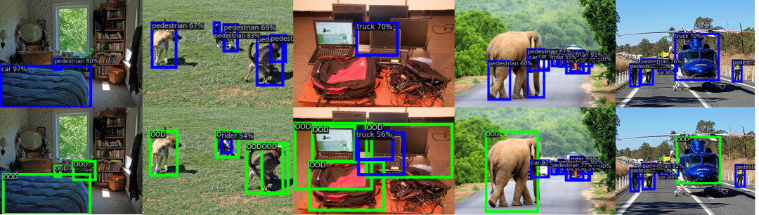
Figure 5: Visualization of detected objects on the OOD images (from MS-COCO) by a vanilla Faster-RCNN (top) and VOS (bottom). The in-distribution is BDD-100k dataset. Blue: Objects detected and classified as one of the ID classes. Green: OOD objects detected by VOS, which reduce false positives among detected objects.

7 Summary

In this chapter, we propose VOS, a novel unknown-aware training framework for OOD detection. Different from methods that require real outlier data, VOS adaptively synthesizes outliers during training by sampling virtual outliers from the low-likelihood region of the class-conditional distributions. The synthesized outliers meaningfully improve the decision boundary between the ID data and OOD data, resulting in superior OOD detection performance while preserving the performance of the ID task. VOS is effective and suitable for both object detection and classification tasks. We hope our work will inspire future research on unknown-aware deep learning in real-world settings.

Chapter 5 Dream the Impossible: Outlier Imagination with Diffusion Models

Publication Statement. This chapter is joint work with Yiyou Sun, Jerry Zhu and Yixuan Li. The paper version of this chapter appeared in NeurIPS’23 (Du et al., 2023).

Abstract. Utilizing auxiliary outlier datasets to regularize the machine learning model has demonstrated promise for out-of-distribution (OOD) detection and safe prediction. Due to the labor intensity in data collection and cleaning, automating outlier data generation has been a long-desired alternative. Despite the appeal, generating photo-realistic outliers in the high dimensional pixel space has been an open challenge for the field. To tackle the problem, this chapter proposes a new framework Dream-ood, which enables imagining photo-realistic outliers by way of diffusion models, provided with only the in-distribution (ID) data and classes. Specifically, Dream-ood learns a text-conditioned latent space based on ID data, and then samples outliers in the low-likelihood region via the latent, which can be decoded into images by the diffusion model. Different from prior works (Du et al., 2022c; tao2023nonparametric), Dream-ood enables visualizing and understanding the imagined outliers, directly in the pixel space. We conduct comprehensive quantitative and qualitative studies to understand the efficacy of Dream-ood, and show that training with the samples generated by Dream-ood can benefit OOD detection performance. Code is publicly available at https://github.com/deeplearning-wisc/dream-ood.

8 Introduction

Out-of-distribution (OOD) detection is critical for deploying machine learning models in the wild, where samples from novel classes can naturally emerge and should be flagged for caution. Concerningly, modern neural networks are shown to produce overconfident and therefore untrustworthy predictions for unknown OOD inputs (nguyen2015deep). To mitigate the issue, recent works have explored training with an auxiliary outlier dataset, where the model is regularized to learn a more conservative decision boundary around in-distribution (ID) data (Hendrycks et al., 2019; Katz-Samuels et al., 2022; liu2020energy; DBLP:conf/icml/MingFL22). These methods have demonstrated encouraging OOD detection performance over the counterparts without auxiliary data.

Despite the promise, preparing auxiliary data can be labor-intensive and inflexible, and necessitates careful human intervention, such as data cleaning, to ensure the auxiliary outlier data does not overlap with the ID data. Automating outlier data generation has thus been a long-desired alternative. Despite the appeal, generating photo-realistic outliers has been extremely challenging due to the high dimensional space. Recent works including VOS and NPOS (Du et al., 2022c; tao2023nonparametric) proposed sampling outliers in the low-dimensional feature space and directly employed the latent-space outliers to regularize the model. However, these latent-space methods do not allow us to understand the outliers in a human-compatible way. Today, the field still lacks an automatic mechanism to generate high-resolution outliers in the pixel space.

In this chapter, we propose a new framework Dream-ood that enables imagining photo-realistic outliers by way of diffusion models, provided with only ID data and classes (see Figure 6). Harnessing the power of diffusion models for outlier imagination is non-trivial, since one cannot easily describe the exponentially many possibilities of outliers using text prompts. It can be particularly challenging to characterize informative outliers that lie on the boundary of ID data, which have been shown to be the most effective in regularizing the ID classifier and its decision boundary (DBLP:conf/icml/MingFL22). After all, it is almost impossible to describe something in words without knowing what it looks like.

Our framework circumvents the above challenges by: (1) learning compact visual representations for the ID data, conditioned on the textual latent space of the diffusion model (Section 10.1), and (2) sampling new visual embeddings in the text-conditioned latent space, which are then decoded to pixel-space images by the diffusion model (Section 10.2). Concretely, to learn the text-conditioned latent space, we train an image classifier to produce image embeddings that have a higher probability to be aligned with the corresponding class token embedding. The resulting feature embeddings thus form a compact and informative distribution that encodes the ID data. Equipped with the text-conditioned latent space, we sample new embeddings from the low-likelihood region, which can be decoded into the images via the diffusion model. The rationale is if the sampled embedding is distributionally far away from the in-distribution embeddings, the generated image will have a large semantic discrepancy from the ID images and vice versa.

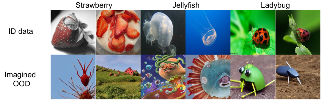
Figure 6: Top: Original ID training data in ImageNet (Deng et al., 2009). Bottom: Samples generated by our method Dream-ood, which deviate from the ID data.

We demonstrate that our proposed framework creatively imagines OOD samples conditioned on a given dataset, and as a result, helps improve the OOD detection performance. On Imagenet dataset, training with samples generated by Dream-ood improves the OOD detection on a comprehensive suite of OOD datasets. Different from (Du et al., 2022c; tao2023nonparametric), our method allows visualizing and understanding the imagined outliers, covering a wide spectrum of near-OOD and far-OOD. Note that Dream-ood enables leveraging off-the-shelf diffusion models for OOD detection, rather than modifying the diffusion model (which is an actively studied area on its own (nichol2021improved)). In other words, this work’s core contribution is to leverage generative modeling to improve discriminative learning, establishing innovative connections between the diffusion model and outlier data generation.

Our key contributions are summarized as follows:

1. To the best of our knowledge, Dream-ood is the first to enable the generation of photo-realistic high-resolution outliers for OOD detection. Dream-ood establishes promising performance on common benchmarks and can benefit OOD detection.

2. We conduct comprehensive analyses to understand the efficacy of Dream-ood, both quantitatively and qualitatively. The results provide insights into outlier imagination with diffusion models.

3. As an extension, we show that our synthesis method can be used to automatically generate ID samples, and as a result, improves the generalization performance of the ID task itself.

9 Preliminaries

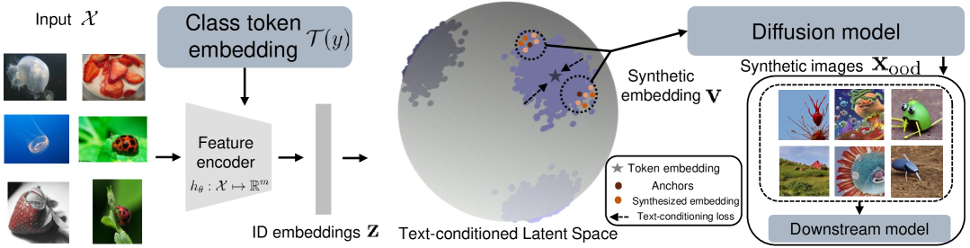
Figure 7: Illustration of our proposed outlier imagination framework Dream-ood. Dream-ood first learns a text-conditioned space to produce compact image embeddings aligned with the token embedding $\mathcal{T}(y)$ of the diffusion model. It then samples new embeddings in the latent space, which can be decoded into pixel-space outlier images $\mathbf{x}_{\text{ood}}$ by diffusion model. The newly generated samples can help improve OOD detection. Best viewed in color.

We consider a training set $\mathcal{D}=\{(\mathbf{x}_{i},y_{i})\}_{i=1}^{n}$, drawn i.i.d. from the joint data distribution $P_{\mathcal{X}\mathcal{Y}}$. $\mathcal{X}$ denotes the input space and $\mathcal{Y}\in\{1,2,...,C\}$ denotes the label space. Let $\mathbb{P}_{\text{in}}$ denote the marginal distribution on $\mathcal{X}$, which is also referred to as the in-distribution. Let $f_{\theta}:\mathcal{X}\mapsto\mathbb{R}^{C}$ denote a multi-class classifier, which predicts the label of an input sample with parameter $\theta$. To obtain an optimal classifier $f^{*}$, a standard approach is to perform empirical risk minimization (ERM) (vapnik1999nature): $f^{*}=\text{argmin}_{f\in\mathcal{F}}\frac{1}{n}\sum_{i=1}^{n}\ell(f(\mathbf{x}_{i}),y_{i})$ where $\ell$ is the loss function and $\mathcal{F}$ is the hypothesis space.

Out-of-distribution detection. When deploying a machine model in the real world, a reliable classifier should not only accurately classify known in-distribution samples, but also identify OOD input from unknown class $y\notin\mathcal{Y}$. This can be achieved by having an OOD detector, in tandem with the classification model $f_{\theta}$. At its core, OOD detection can be formulated as a binary classification problem. At test time, the goal is to decide whether a test-time input is from ID or not (OOD). We denote $g_{\theta}:\mathcal{X}\mapsto\{\text{in},\text{out}\}$ as the function mapping for OOD detection.

Denoising diffusion models have emerged as a promising generative modeling framework, pushing the state-of-the-art in image generation (ramesh2022hierarchical; saharia2022photorealistic). Inspired by non-equilibrium thermodynamics, diffusion probabilistic models (sohl2015deep; song2020denoising; Ho et al., 2020) define a forward Gaussian Markov transition kernel of diffusion steps to gradually corrupt training data until the data distribution is transformed into a simple noisy distribution. The model then learns to reverse this process by learning a denoising transition kernel parameterized by a neural network.

Diffusion models can be conditional, for example, on class labels or text descriptions (ramesh2022hierarchical; nichol2021glide; saharia2022image). In particular, Stable Diffusion (rombach2022high) is a text-to-image model that enables synthesizing new images guided by the text prompt. The model was trained on 5 billion pairs of images and captions taken from LAION-5B (schuhmann2022laion), a publicly available dataset derived from Common Crawl data scraped from the web. Given a class name $y$, the generation process can be mathematically denoted by:

$$\mathbf{x}\sim P(\mathbf{x}|\mathbf{z}_{y}),$$ (16)

where $\mathbf{z}_{y}=\mathcal{T}(y)$ is the textual representation of label $y$ with prompting (e.g., ‘‘A high-quality photo of a [$y$]’’). In Stable Diffusion, $\mathcal{T}(\cdot)$ is the text encoder of the CLIP model (radford2021learning).

10 Dream-ood: Outlier Imagination with Diffusion Models

In this chapter, we propose a novel framework that enables synthesizing photo-realistic outliers with respect to a given ID dataset (see Figure 6). The synthesized outliers can be useful for regularizing the ID classifier to be less confident in the OOD region. Recall that the vanilla diffusion generation takes as input the textual representation. While it is easy to encode the ID classes $y\in\mathcal{Y}$ into textual latent space via $\mathcal{T}(y)$, one cannot trivially generate text prompts for outliers. It can be particularly challenging to characterize informative outliers that lie on the boundary of ID data, which have been shown to be most effective in regularizing the ID classifier and its decision boundary (DBLP:conf/icml/MingFL22). After all, it is almost impossible to concretely describe something in words without knowing what it looks like.

Overview.

As illustrated in Figure 14, our framework circumvents the challenge by: (1) learning compact visual representations for the ID data, conditioned on the textual latent space of the diffusion model (Section 10.1), and (2) sampling new visual embeddings in the text-conditioned latent space, which are then decoded into the images by diffusion model (Section 10.2). We demonstrate in Section 11 that, our proposed outlier synthesis framework produces meaningful out-of-distribution samples conditioned on a given dataset, and as a result, significantly improves the OOD detection performance.

10.1 Learning the Text-Conditioned Latent Space

Our key idea is to first train a classifier on ID data $\mathcal{D}$ that produces image embeddings, conditioned on the token embeddings $\mathcal{T}(y)$, with $y\in\mathcal{Y}$. To learn the text-conditioned visual latent space, we train the image classifier to produce image embeddings that have a higher probability of being aligned with the corresponding class token embedding, and vice versa.

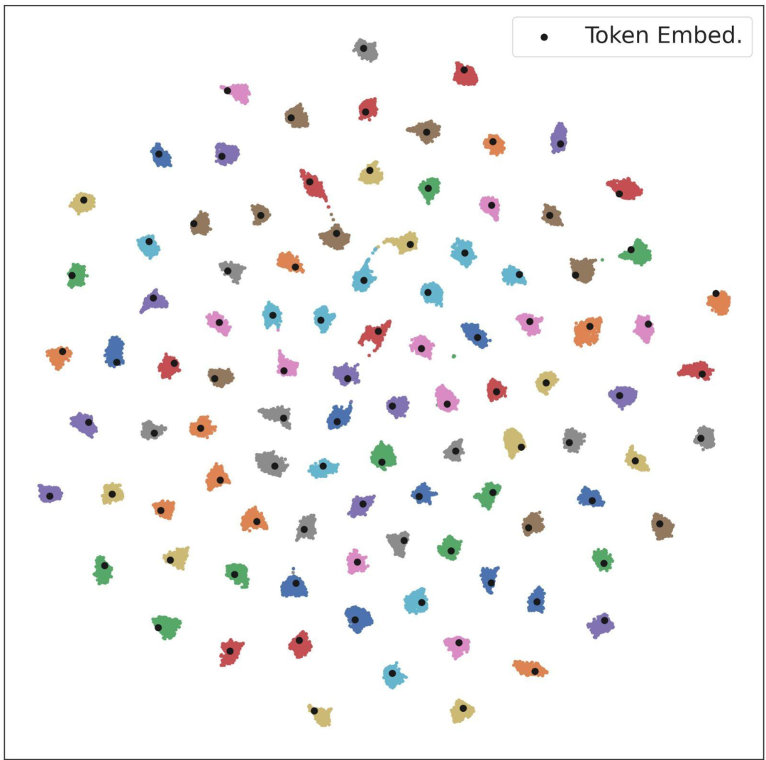
Figure 8: TSNE visualization of learned feature embeddings using $\mathcal{L}$. Black dots indicate token embeddings, one for each class.

Specifically, denote $h_{\theta}:\mathcal{X}\mapsto\mathbb{R}^{m}$ as a feature encoder that maps an input $\mathbf{x}\in\mathcal{X}$ to the image embedding $h_{\theta}(\mathbf{x})$, and $\mathcal{T}:\mathcal{Y}\mapsto\mathbb{R}^{m}$ as the text encoder that takes a class name $y$ and outputs its token embedding $\mathcal{T}(y)$. Here $\mathcal{T}(\cdot)$ is a fixed text encoder of the diffusion model. Only the image feature encoder needs to be trained, with learnable parameters $\theta$. Mathematically, the loss function for learning the visual representations is formulated as follows:

$$\mathcal{L}=\mathbb{E}_{(\mathbf{x},y)\sim\mathcal{D}}[-\log\frac{\exp\left(\mathcal{T}(y)^{\top}\mathbf{z}/t\right)}{\sum_{j=1}^{C}\exp\left(\mathcal{T}(y_{j})^{\top}\mathbf{z}/t\right)}],$$ (17)

where $\mathbf{z}=h_{\theta}(\mathbf{x})/\|h_{\theta}(\mathbf{x})\|_{2}$ is the $L_{2}$-normalized image embedding, and $t$ is temperature.

Theoretical interpretation of loss. Formally, our loss function directly promotes the class-conditional von Mises Fisher (vMF) distribution (Du et al., 2022a; mardia2000directional; ming2023cider). vMF is analogous to spherical Gaussian distributions for features with unit norms ($\|\mathbf{z}\|^{2}=1$). The probability density function of $\mathbf{z}\in\mathbb{R}^{m}$ in class $c$ is:

$$p_{m}(\mathbf{z};\boldsymbol{\mu}_{c},\kappa)=Z_{m}(\kappa)\exp\left(\kappa\boldsymbol{\mu}_{c}^{\top}\mathbf{z}\right),$$ (18)

where $\boldsymbol{\mu}_{c}$ is the class centroid with unit norm, $\kappa\geq 0$ controls the extent of class concentration, and $Z_{m}(\kappa)$ is the normalization factor detailed in the Appendix 31.2. The probability of the feature vector $\mathbf{z}$ belonging to class $c$ is:

$${P}(y=c|\mathbf{z};\{\kappa,\boldsymbol{\mu}_{j}\}_{j=1}^{C}) =\frac{Z_{m}\left(\kappa\right)\exp\left(\kappa\boldsymbol{\mu}_{c}^{\top}\mathbf{z}\right)}{\sum_{j=1}^{C}Z_{m}\left(\kappa\right)\exp\left(\kappa\boldsymbol{\mu}_{j}^{\top}\mathbf{z}\right)}$$

$$=\frac{\exp\left(\boldsymbol{\mu}_{c}^{\top}\mathbf{z}/t\right)}{\sum_{j=1}^{C}\exp\left(\boldsymbol{\mu}_{j}^{\top}\mathbf{z}/t\right)},$$ (19)

where $\kappa={1\over t}$. Therefore, by encouraging features to be aligned with its class token embedding, our loss function $\mathcal{L}$ (Equation (17)) maximizes the log-likelihood of the class-conditional vMF distributions and promotes compact clusters on the hypersphere (see Figure 8). The highly compact representations can benefit the sampling of new embeddings, as we introduce next in Section 10.2.

10.2 Outlier Imagination via Text-Conditioned Latent

Given the well-trained compact representation space that encodes the information of $\mathbb{P}_{\text{in}}$, we propose to generate outliers by sampling new embeddings in the text-conditioned latent space, and then decoding via diffusion model. The rationale is that if the sampled embeddings are distributionally far away from the ID embeddings, the decoded images will have a large semantic discrepancy with the ID images and vice versa.

Recent works (Du et al., 2022c; tao2023nonparametric) proposed sampling outlier embeddings and directly employed the latent-space outliers to regularize the model. In contrast, our method focuses on generating pixel-space photo-realistic images, which allows us to directly inspect the generated outliers in a human-compatible way. Despite the appeal, generating high-resolution outliers has been extremely challenging due to the high dimensional space. To tackle the issue, our generation procedure constitutes two steps:

1. Sample OOD in the latent space: draw new embeddings $\mathbf{v}$ that are in the low-likelihood region of the text-conditioned latent space.

2. Image generation: decode $\mathbf{v}$ into a pixel-space OOD image via diffusion model.

Input: In-distribution training data $\mathcal{D}=\left\{\left(\mathbf{x}_{i},{y}_{i}\right)\right\}_{i=1}^{n}$, initial model parameters ${\theta}$ for learning the text-conditioned latent space, diffusion model.

Output: Synthetic images $\mathbf{x}_{\text{ood}}$.

Phases: Phase 1: Learning the Text-conditioned Latent Space. Phase 2: Outlier Imagination via Text-Conditioned Latent.

while Phase 1 do

    1. Extract token embeddings $\mathcal{T}(y)$ of the ID label $y\in\mathcal{Y}$.

    2. Learn the text-conditioned latent representation space by Equation (17).

end while

while Phase 2 do

    1. Sample a set of outlier embeddings $V_{i}$ in the low-likelihood region of the text-conditioned latent space as in Section 10.2.

    2. Decode the outlier embeddings into the pixel-space OOD images via diffusion model by Equation (21).

end while

Algorithm 2 Dream-ood: Outlier Imagination with Diffusion Models

Figure 9: TSNE visualization of ID embeddings (purple) and the sampled outlier embeddings (orange), for the class ‘‘hen" in Imagenet.

Sampling OOD embedding. Our goal here is to sample low-likelihood embeddings based on the learned feature representations (see Figure 9). The sampling procedure can be instantiated by different approaches. For example, a recent work by  tao2023nonparametric proposed a latent non-parametric sampling method, which does not make any distributional assumption on the ID embeddings and offers stronger flexibility compared to the parametric sampling approach (Du et al., 2022c). Concretely, we can select the boundary ID anchors by leveraging the non-parametric nearest neighbor distance, and then draw new embeddings around that boundary point.

Denote the $L_{2}$-normalized embedding set of training data as $\mathbb{Z}=(\mathbf{z}_{1},\mathbf{z}_{2},...,\mathbf{z}_{n})$, where $\mathbf{z}_{i}=h_{\theta}(\mathbf{x}_{i})/\|h_{\theta}(\mathbf{x}_{i})\|_{2}$. For any embedding $\mathbf{z}^{\prime}\in\mathbb{Z}$, we calculate the $k$-NN distance w.r.t. $\mathbb{Z}$:

$$d_{k}(\mathbf{z}^{\prime},\mathbb{Z})=\lVert\mathbf{z}^{\prime}-\mathbf{z}_{(k)}\rVert_{2},$$ (20)

where $\mathbf{z}_{(k)}$ is the $k$-th nearest neighbor in $\mathbb{Z}$. If an embedding has a large $k$-NN distance, it is likely to be on the boundary of the ID data and vice versa.

Given a boundary ID point, we then draw new embedding sample $\mathbf{v}\in\mathbb{R}^{m}$ from a Gaussian kernel centered at $\mathbf{z}_{i}$ with covariance $\sigma^{2}\mathbf{I}$: $\mathbf{v}\sim\mathcal{N}(\mathbf{z}_{i},\sigma^{2}\mathbf{I})$. In addition, to ensure that the outliers are sufficiently far away from the ID data, we repeatedly sample multiple outlier embeddings from the Gaussian kernel $\mathcal{N}(\mathbf{z}_{i},\sigma^{2}\mathbf{I})$, which produces a set $V_{i}$, and further perform a filtering process by selecting the outlier embedding in $V_{i}$ with the largest $k$-NN distance w.r.t. $\mathbb{Z}$. Detailed ablations on the sampling parameters are provided in Section 11.2.

Outlier image generation.

Lastly, to obtain the outlier images in the pixel space, we decode the sampled outlier embeddings $\mathbf{v}$ via the diffusion model. In practice, this can be done by replacing the original token embedding $\mathcal{T}(y)$ with the sampled new embedding $\mathbf{v}$. Different from the vanilla prompt-based generation (c.f. Equation (16)) , our outlier imagination is mathematically reflected by:

$$\mathbf{x}_{\text{ood}}\sim P(\mathbf{x}|\mathbf{v}),$$ (21)

where ${\mathbf{x}}_{\text{ood}}$ denotes the generated outliers in the pixel space. Importantly, $\mathbf{v}\sim S\circ h_{\theta}\circ(\mathbb{P}_{\text{in}})$ is dependent on the in-distribution data, which enables generating images that deviate from $\mathbb{P}_{\text{in}}$. $S(\cdot)$ denotes the sampling procedure. Our framework Dream-ood is summarized in Algorithm 2.

Learning with imagined outlier images. The generated synthetic OOD images $\mathbf{x}_{\text{ood}}$ can be used for regularizing the training of the classification model (Du et al., 2022c):

$$\mathcal{L}_{\text{ood}}=\mathbb{E}_{\mathbf{x}_{\text{ood}}}\left[-\log\frac{1}{1+\exp^{\phi(E(f_{\theta}(\mathbf{x}_{\text{ood}})))}}\right]+\mathbb{E}_{\mathbf{x}\sim\mathbb{P}_{\text{in}}}\left[-\log\frac{\exp^{\phi(E(f_{\theta}(\mathbf{x})))}}{1+\exp^{\phi(E(f_{\theta}(\mathbf{x})))}}\right],$$ (22)

where $\phi(\cdot)$ is a three-layer nonlinear MLP function with the same architecture as VOS (Du et al., 2022c), $E(\cdot)$ denotes the energy function, and $f_{\theta}(\mathbf{x})$ denotes the logit output of the classification model. In other words, the loss function takes both the ID and generated OOD images, and learns to separate them explicitly. The overall training objective combines the standard cross-entropy loss, along with an additional loss in terms of OOD regularization $\mathcal{L}_{\text{CE}}+\beta\cdot\mathcal{L}_{\text{ood}}$, where $\beta$ is the weight of the OOD regularization. $\mathcal{L}_{\text{CE}}$ denotes the cross-entropy loss on the ID training data. In testing, we use the output of the binary logistic classifier for OOD detection.

11 Experiments and Analysis

In this section, we present empirical evidence to validate the effectiveness of our proposed outlier imagination framework. In what follows, we show that Dream-ood produces meaningful OOD images, and as a result, significantly improves OOD detection (Section 11.1) performance. We provide comprehensive ablations and qualitative studies in Section 11.2. In addition, we showcase an extension of our framework for improving generalization by leveraging the synthesized inliers (Section 11.3).

11.1 Evaluation on OOD Detection Performance

Methods	OOD Datasets										ID ACC
	iNaturalist		Places		Sun		Textures		Average
	FPR95$\downarrow$	AUROC$\uparrow$	FPR95$\downarrow$	AUROC$\uparrow$	FPR95$\downarrow$	AUROC$\uparrow$	FPR95$\downarrow$	AUROC$\uparrow$	FPR95$\downarrow$	AUROC$\uparrow$
MSP (Hendrycks and Gimpel, 2017)	31.80	94.98	47.10	90.84	47.60	90.86	65.80	83.34	48.08	90.01	87.64
ODIN (liang2018enhancing)	24.40	95.92	50.30	90.20	44.90	91.55	61.00	81.37	45.15	89.76	87.64
Mahalanobis (lee2018simple)	91.60	75.16	96.70	60.87	97.40	62.23	36.50	91.43	80.55	72.42	87.64
Energy (liu2020energy)	32.50	94.82	50.80	90.76	47.60	91.71	63.80	80.54	48.68	89.46	87.64
GODIN (Hsu et al., 2020)	39.90	93.94	59.70	89.20	58.70	90.65	39.90	92.71	49.55	91.62	87.38
KNN (sun2022out)	28.67	95.57	65.83	88.72	58.08	90.17	12.92	90.37	41.38	91.20	87.64
ViM (wang2022vim)	75.50	87.18	88.30	81.25	88.70	81.37	15.60	96.63	67.03	86.61	87.64
ReAct (sun2021react)	22.40	96.05	45.10	92.28	37.90	93.04	59.30	85.19	41.17	91.64	87.64
DICE (sun2022dice)	37.30	92.51	53.80	87.75	45.60	89.21	50.00	83.27	46.67	88.19	87.64
Synthesis-based methods
GAN (lee2018training)	83.10	71.35	83.20	69.85	84.40	67.56	91.00	59.16	85.42	66.98	79.52
VOS (Du et al., 2022c)	43.00	93.77	47.60	91.77	39.40	93.17	66.10	81.42	49.02	90.03	87.50
NPOS (tao2023nonparametric)	53.84	86.52	59.66	83.50	53.54	87.99	8.98	98.13	44.00	89.04	85.37
Dream-ood (Ours)	24.10$\pm$0.2	96.10$\pm$0.1	39.87$\pm$0.1	93.11$\pm$0.3	36.88$\pm$0.4	93.31$\pm$0.4	53.99$\pm$0.6	85.56$\pm$0.9	38.76$\pm$0.2	92.02$\pm$0.4	87.54$\pm$0.1

Table 5: OOD detection results for Imagenet-100 as the in-distribution data. We report standard deviations estimated across 3 runs. Bold numbers are superior results.

Datasets. Following  tao2023nonparametric, we use the Cifar-100 and the large-scale Imagenet dataset (Deng et al., 2009) as the ID training data. For Cifar-100, we use a suite of natural image datasets as OOD including Textures (Cimpoi et al., 2014), Svhn (netzer2011reading), Places365 (zhou2017places), iSun (DBLP:journals/corr/XuEZFKX15) & Lsun (DBLP:journals/corr/YuZSSX15). For Imagenet-100, we adopt the OOD test data as in (Huang and Li, 2021), including subsets of iNaturalist (van2018inaturalist), Sun (xiao2010sun), Places (zhou2017places), and Textures (Cimpoi et al., 2014). For each OOD dataset, the categories are disjoint from the ID dataset. We provide the details of the datasets and categories in Appendix 31.1.

Training details. We use ResNet-34 (He et al., 2016a) as the network architecture for both Cifar-100 and Imagenet-100 datasets. We train the model using stochastic gradient descent for 100 epochs with the cosine learning rate decay schedule, a momentum of 0.9, and a weight decay of $5e^{-4}$. The initial learning rate is set to 0.1 and the batch size is set to 160. We generate $1,000$ OOD samples per class using Stable Diffusion v1.4, which results in $100,000$ synthetic images in total. $\beta$ is set to 1.0 for ImageNet-100 and 2.5 for Cifar-100. To learn the feature encoder $h_{\theta}$, we set the temperature $t$ in Equation (17) to 0.1. Extensive ablations on hyperparameters $\sigma$, $k$ and $\beta$ are provided in Section 11.2.

Evaluation metrics. We report the following metrics: (1) the false positive rate (FPR95) of OOD samples when the true positive rate of ID samples is 95%, (2) the area under the receiver operating characteristic curve (AUROC), and (3) ID accuracy (ID ACC).

Dream-ood significantly improves the OOD detection performance. As shown in Table 5 and Table 7, we compare our method with the competitive baselines, including Maximum Softmax Probability (Hendrycks and Gimpel, 2017), ODIN score (liang2018enhancing), Mahalanobis score (lee2018simple), Energy score (liu2020energy), Generalized ODIN (Hsu et al., 2020), KNN distance (sun2022out), ViM score (wang2022vim), ReAct (sun2021react), and DICE (sun2022dice). Closely related to ours, we contrast with three synthesis-based methods, including latent-based outlier synthesis (VOS (Du et al., 2022c) & NPOS (tao2023nonparametric)), and GAN-based synthesis (lee2018training), showcasing the effectiveness of our approach. For example, Dream-ood achieves an FPR95 of 39.87% on Places with the ID data of Imagenet-100, which is a 19.79% improvement from the best baseline NPOS.

In particular, Dream-ood advances both VOS and NPOS by allowing us to understand the synthesized outliers in a human-compatible way, which was infeasible for the feature-based outlier sampling in VOS and NPOS. Compared with the feature-based synthesis approaches, Dream-ood can generate high-resolution outliers in the pixel space. The higher-dimensional pixel space offers much more knowledge about the unknowns, which provides the model with high variability and fine-grained details for the unknowns that are missing in VOS and NPOS. Since Dream-ood is more photo-realistic and better for humans, the generated images can be naturally better constrained for neural networks (for example, things may be more on the natural image manifolds). We provide comprehensive qualitative results (Section 11.2) to facilitate the understanding of generated outliers. As we will show in Figure 10, the generated outliers are more precise in characterizing OOD data and thus improve the empirical performance.

Method	FPR95 $\downarrow$	AUROC $\uparrow$	FPR95 $\downarrow$	AUROC $\uparrow$
	Imagenet-100 as ID		Cifar-100 as ID
(I) Add gaussian noise	41.35	89.91	45.33	88.83
(II) Add learnable noise	42.48	91.45	48.05	87.72
(III) Interpolate embeddings	41.35	90.82	43.36	87.09
(IV) Disjont class names	43.55	87.84	49.89	85.87
Dream-ood (ours)	38.76	92.02	40.31	90.15

Table 6: Comparison of Dream-ood with different outlier embedding synthesis methods using diffusion models.

Comparison with other outlier synthesis approaches.

We compare Dream-ood with different outlier embedding synthesis approaches in Table 6: (I) synthesizing outlier embeddings by adding multivariate Gaussian noise $\mathcal{N}(\textbf{0},\sigma_{1}^{2}\mathbf{I})$ to the token embeddings, (II) adding learnable noise to the token embeddings where the noise is trained to push the outliers away from ID features, (III) interpolating token embeddings from different classes by $\alpha\mathcal{T}(y_{1})+(1-\alpha)\mathcal{T}(y_{2})$, and (IV) generating outlier images by using embeddings of new class names outside ID classes. For (I), we set the optimal variance values $\sigma_{1}^{2}$ to 0.03 by sweeping from $\{0.01,0.02,0.03,...,0.10\}$. For (III), we choose the interpolation factor $\alpha$ to be $0.5$ from $\{0.1,0.2,...,0.9\}$. For (IV), we use the remaining 900 classes in Imagenet-1k (exclude the 100 classes in Imagenet-100) as the disjoint class names for outlier generation. We generate the same amount of images as ours for all the variants to ensure a fair comparison.

Methods	OOD Datasets												ID ACC
	Svhn		Places365		Lsun		iSun		Textures		Average
	FPR95$\downarrow$	AUROC$\uparrow$	FPR95$\downarrow$	AUROC$\uparrow$	FPR95$\downarrow$	AUROC$\uparrow$	FPR95$\downarrow$	AUROC$\uparrow$	FPR95$\downarrow$	AUROC$\uparrow$	FPR95$\downarrow$	AUROC$\uparrow$
MSP (Hendrycks and Gimpel, 2017)	87.35	69.08	81.65	76.71	76.40	80.12	76.00	78.90	79.35	77.43	80.15	76.45	79.04
ODIN (liang2018enhancing)	90.95	64.36	79.30	74.87	75.60	78.04	53.10	87.40	72.60	79.82	74.31	76.90	79.04
Mahalanobis (lee2018simple)	87.80	69.98	76.00	77.90	56.80	85.83	59.20	86.46	62.45	84.43	68.45	80.92	79.04
Energy (liu2020energy)	84.90	70.90	82.05	76.00	81.75	78.36	73.55	81.20	78.70	78.87	80.19	77.07	79.04
GODIN (Hsu et al., 2020)	63.95	88.98	80.65	77.19	60.65	88.36	51.60	92.07	71.75	85.02	65.72	86.32	76.34
KNN (sun2022out)	81.12	73.65	79.62	78.21	63.29	85.56	73.92	79.77	73.29	80.35	74.25	79.51	79.04
ViM (wang2022vim)	81.20	77.24	79.20	77.81	43.10	90.43	74.55	83.02	61.85	85.57	67.98	82.81	79.04
ReAct (sun2021react)	82.85	70.12	81.75	76.25	80.70	83.03	67.40	83.28	74.60	81.61	77.46	78.86	79.04
DICE (sun2022dice)	83.55	72.49	85.05	75.92	94.05	73.59	75.20	80.90	79.80	77.83	83.53	76.15	79.04
Synthesis-based methods
GAN (lee2018training)	89.45	66.95	88.75	66.76	82.35	75.87	83.45	73.49	92.80	62.99	87.36	69.21	70.12
VOS (Du et al., 2022c)	78.50	73.11	84.55	75.85	59.05	85.72	72.45	82.66	75.35	80.08	73.98	79.48	78.56
NPOS (tao2023nonparametric)	11.14	97.84	79.08	71.30	56.27	82.43	51.72	85.48	35.20	92.44	46.68	85.90	78.23
Dream-ood (Ours)	58.75$\pm$0.6	87.01$\pm$0.1	70.85$\pm$1.6	79.94$\pm$0.2	24.25$\pm$1.1	95.23$\pm$0.2	1.10$\pm$0.2	99.73$\pm$0.4	46.60$\pm$0.4	88.82$\pm$0.7	40.31$\pm$0.8	90.15$\pm$0.3	78.94

Table 7: OOD detection results for Cifar-100 as the in-distribution data. We report standard deviations estimated across 3 runs. Bold numbers are superior results.

The result shows that Dream-ood outperforms all the alternative synthesis approaches by a considerable margin. Though adding noise to the token embedding is relatively simple, it cannot explicitly sample textual embeddings from the low-likelihood region as Dream-ood does, which are near the ID boundary and thus demonstrate stronger effectiveness to regularize the model (Section 10.2). Visualization is provided in Appendix 31.5. Interpolating the token embeddings will easily generate images that are still ID (Appendix 31.4), which is also observed in (liew2022magicmix).

11.2 Ablation Studies

In this section, we provide additional ablations to understand Dream-ood for OOD generation. For all the ablations, we use the high resolution Imagenet-100 dataset as the ID data.

Ablation on the regularization weight $\beta$. In Figure 12 (a), we ablate the effect of weight $\beta$ of the regularization loss $\mathcal{L}_{\text{ood}}$ for OOD detection (Section 10.2) on the OOD detection performance. Using a mild weighting, such as $\beta$ = 1.0, achieves the best OOD detection performance. Too excessive regularization using synthesized OOD images ultimately degrades the performance.

Ablation on the variance value $\sigma^{2}$. We show in Figure 12 (b) the effect of $\sigma^{2}$ — the number of the variance value for the Gaussian kernel (Section 10.2). We vary $\sigma^{2}\in\{0.02,0.03,0.04,0.05,0.06,0.2\}$. Using a mild variance value $\sigma^{2}$ generates meaningful synthetic OOD images for model regularization. Too large of variance (e.g., $\sigma^{2}=0.2$) produces far-OOD, which does not help learn a compact decision boundary between ID and OOD.

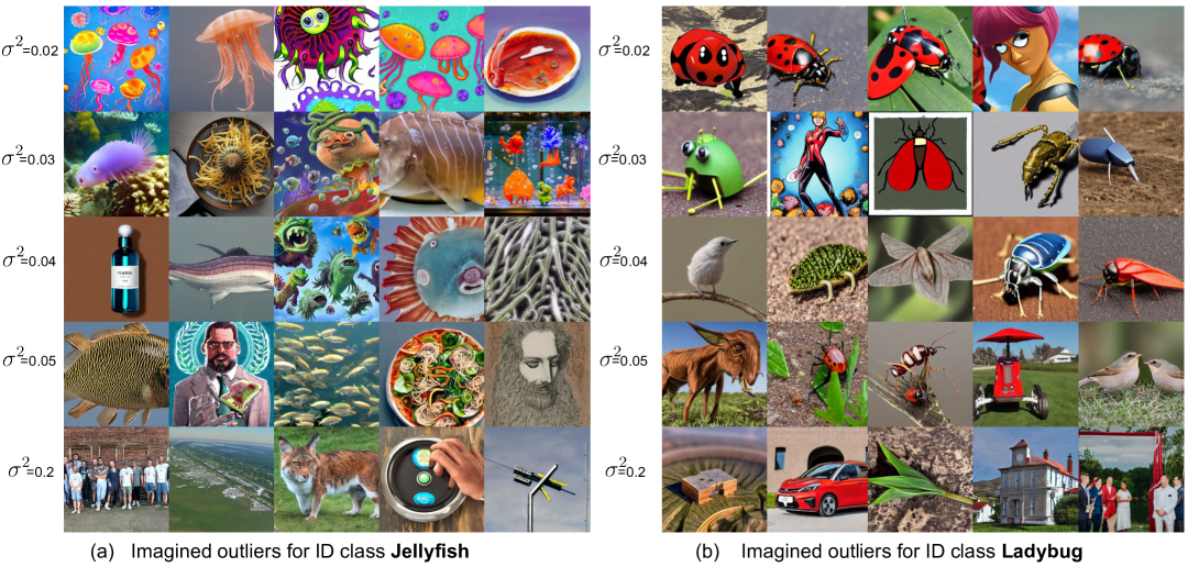
Figure 10: Visualization of the imagined outliers w.r.t. jellyfish, ladybug class under different variance $\sigma^{2}$.

Ablation on $k$ in calculating $k$-NN distance. In Figure 12 (c), we analyze the effect of $k$, i.e., the number of nearest neighbors for non-parametric sampling in the latent space. We vary $k=\{100,200,300,400,500\}$ and observe that our method is not sensitive to this hyperparameter.

Visualization of the generated outliers. Figure 10 illustrates the generated outlier images under different variance $\sigma^{2}$. Mathematically, a larger variance translates into outliers that are more deviated from ID data. We confirm this in our visualization too. The synthetic OOD images gradually become semantically different from ID classes ‘‘jellyfish’’ and ‘‘ladybug’’, as the variance increases. More visualization results are in Appendix 31.3.

11.3 Extension: from Dream-ood to Dream-id

Our framework can be easily extended to generate ID data. Specifically, we can select the ID point with small $k$-NN distances w.r.t. the training data (Equation (20)) and sample inliers from the Gaussian kernel with small variance $\sigma^{2}$ in the text-conditioned embedding space (Figure 11). Then we decode the inlier embeddings via the diffusion model for ID generation (Visualization provided in Appendix 31.7). For the synthesized ID images, we let the semantic label be the same as the anchor ID point. Here we term our extension as Dream-id instead.

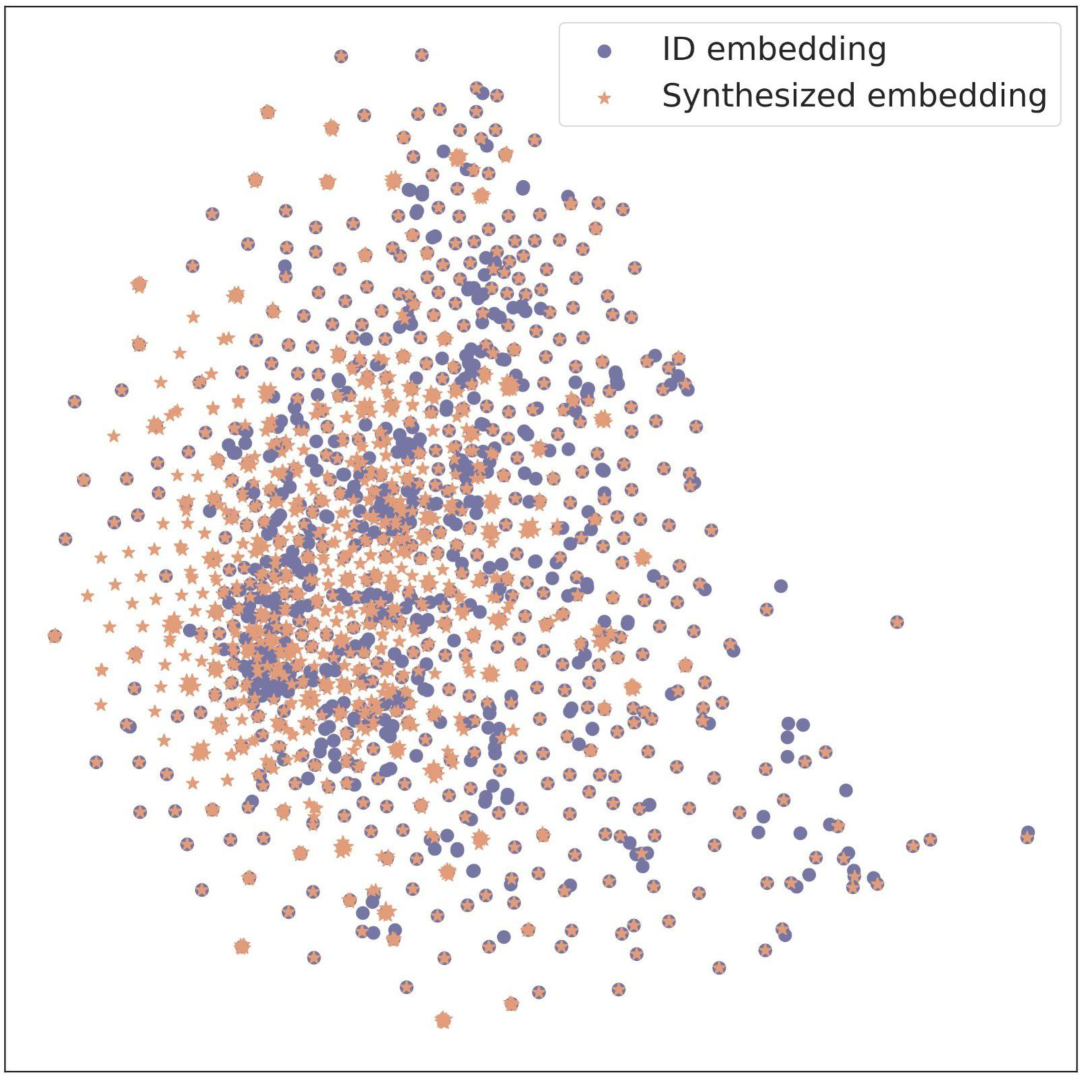
Figure 11: TSNE visualization of ID embeddings (purple) and the synthesized inlier embeddings (orange), for class ‘‘hen’’ in Imagenet.

Datasets. We use the same Imagenet-100 as the training data. We measure the generalization performance on both the original Imagenet test data (for ID generalization) and variants with distribution shifts (for OOD generalization). For OOD generalization, we evaluate on (1) Imagenet-a (Hendrycks et al., 2021b) consisting of real-world, unmodified, and naturally occurring examples that are misclassified by ResNet models; (2) Imagenet-v2 (recht2019imagenet), which is created from the Flickr dataset with natural distribution shifts. We provide the experimental details in Appendix 31.8.

Dream-id improves the generalization performance. As shown in Table 8, we compare Dream-id with competitive data augmentation and test-time adaptation methods. For a fair comparison, all the methods are trained using the same network architecture, under the same configuration. Specifically, our baselines include: the original model without any data augmentation, RandAugment (Cubuk et al., 2020), AutoAugment (Cubuk et al., 2019), CutMix (yun2019cutmix), AugMix (Hendrycks* et al., 2020), DeepAugment (Hendrycks et al., 2021a) and MEMO (zhang2021memo). These methods are shown in the literature to help improve generalization. The results demonstrate that our approach outperforms all the baselines that use data augmentation for training in both ID generalization and generalization under natural distribution shifts ($\uparrow$0.74% vs. the best on Imagenet-a, $\uparrow$0.70% vs. the best on Imagenet-v2). Implementation details of the baselines are in Appendix 31.9.

Methods	Imagenet	Imagenet-A	Imagenet-v2
Original (no aug)	87.28	8.69	77.80
RandAugment	88.10	11.39	78.90
AutoAugment	88.00	10.85	79.70
CutMix	87.98	9.67	79.70
AugMix	87.74	10.96	79.20
DeepAugment	86.86	10.79	78.30
MEMO	88.00	10.85	78.60
Generic Prompts	87.74	11.18	79.20
Dream-id (Ours)	88.46$\pm$0.1	12.13$\pm$0.1	80.40$\pm$0.1

Table 8: Model generalization performance (accuracy, in %), using Imagenet-100 as the training data. We report standard deviations estimated across 3 runs.

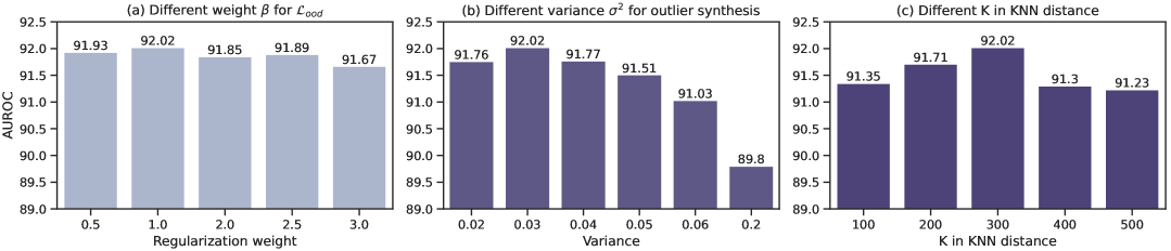
Figure 12: (a) Ablation study on the regularization weight $\beta$ on $\mathcal{L}_{\textrm{ood}}$. (b) Ablation on the variance $\sigma^{2}$ for synthesizing outliers in Section 10.2. (c) Ablation on the $k$ for the $k$-NN distance. The numbers are AUROC. The ID training dataset is Imagenet-100.

In addition, we compare our method with using generic prompts (i.e., ‘‘A high-quality photo of a [$y$]’’) for data generation. For a fair comparison, we synthesize the same amount of images (i.e., $1000$ per class) for both methods. The result shows that Dream-id outperforms the baseline by $0.72\%$ on Imagenet test set and $0.95\%,1.20\%$ on Imagenet-a and Imagenet-v2, respectively.

12 Summary

In this chapter, we propose a novel learning framework Dream-ood, which imagines photo-realistic outliers in the pixel space by way of diffusion models. Dream-ood mitigates the key shortcomings of training with auxiliary outlier datasets, which typically require label-intensive human intervention for data preparation. Dream-ood learns a text-conditioned latent space based on ID data, and then samples outliers in the low-likelihood region via the latent. We then generate outlier images by decoding the outlier embeddings with the diffusion model. The empirical result shows that training with the outlier images helps establish competitive performance on common OOD detection benchmarks. Our in-depth quantitative and qualitative ablations provide further insights on the efficacy of Dream-ood. We hope our work will inspire future research on automatic outlier synthesis in the pixel space.

Chapter 6 SIREN: Shaping Representations for Detecting Out-of-Distribution Objects

Publication Statement. This chapter is joint work with Gabriel Gozum, Yifei Ming and Yixuan Li. The paper version of this chapter appeared in NeurIPS’22 (Du et al., 2022a).

Abstract. Detecting out-of-distribution (OOD) objects is indispensable for safely deploying object detectors in the wild. Although distance-based OOD detection methods have demonstrated promise in image classification, they remain largely unexplored in object-level OOD detection. This chapter bridges the gap by proposing a distance-based framework for detecting OOD objects, which relies on the model-agnostic representation space and provides strong generality across different neural architectures. Our proposed framework Siren contributes two novel components: (1) a representation learning component that uses a trainable loss function to shape the representations into a mixture of von Mises-Fisher (vMF) distributions on the unit hypersphere, and (2) a test-time OOD detection score leveraging the learned vMF distributions in a parametric or non-parametric way. Siren achieves competitive performance on both the recent detection transformers and CNN-based models, improving the AUROC by a large margin compared to the previous best method. Code is publicly available at https://github.com/deeplearning-wisc/siren.

13 Introduction

Teaching object detectors to be aware of out-of-distribution (OOD) data is indispensable for building reliable AI systems. Today, the mainstream object detection models have been operating in the closed-world setting. That is, a model will match an object to one of the given class labels, even if it is irrelevant. Instead, the open-world setting emphasizes that objects from the unknown classes can naturally emerge, which should not be blindly predicted into a known class. In safety-critical applications, such as autonomous driving, failing to detect OOD objects on the road can directly lead to disastrous accidents (DBLP:conf/itsc/NitschISNSSKC21). The situation can be better avoided if the object detector recognizes the object as unfamiliar and appropriately cautions the human driver to take over.

In this chapter, we pioneer a distance-based framework for detecting OOD objects. Currently, the distance-based method remains largely unexplored in object-level OOD detection. In particular, by operating in the representation space, distance-based methods are model-agnostic and provide strong generality across neural architectures. In contrast, existing approaches derive highly specialized OOD detection scores based on the outputs of the object detectors, which may not be seamlessly applicable across architectures. For example, the classification output of the Faster R-CNN (ren2015faster) is optimized by the multi-class softmax loss, whereas the recent transformer-based object detection networks such as deformable-detr (deformable_detr) uses multi-label focal loss (DBLP:journals/pami/LinGGHD20). Thereby, while output-based OOD scoring functions may be limited to specific architectures, distance-based methods are not.

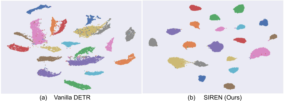
Figure 13: (a) Feature embeddings from the penultimate layer of a vanilla deformable-detr deformable_detr trained on the pascal-voc dataset Everingham et al. (2010), which display irregular distributions. (b) Feature embeddings shaped by the proposed Siren, which form compact clusters on the unit hypersphere.

Although distance-based OOD scoring functions have been studied in image classification, they do not trivially transfer to object detection models. For example, lee2018simple modeled the feature embedding space as a mixture of multivariate Gaussian distributions and used the maximum Mahalanobis distance (mahalanobis1936generalized) to all class centroids for OOD detection. However, we observe that the modern object detection models such as deformable-detr (deformable_detr) produce highly irregular embeddings (Figure 13 (a)), which do not fit the Gaussian distributional assumption. As a result, the OOD detection score relying on such suboptimal embeddings can misbehave.

We propose a novel framework called siren, tackling two highly dependent problems—representation learning and OOD detection—in one synergistic framework. Concretely, Siren contributes two novel components: (1) We introduce an end-to-end trainable loss that enables ShapIng the RepresENtations into a desired parametric form (Section 15.1). In particular, we model the representations by the von Mises-Fisher (vMF) distribution, a classic probability distribution in directional statistics for hyperspherical data with the unit norm. Our loss function encourages the normalized embedding to be aligned with its class prototype and shapes the overall representations into compact clusters for each class. Compared to the Gaussian distribution, using the vMF distribution avoids estimating large covariance matrices for high-dimensional data that is shown to be costly and unstable (Chen et al., 2017; DBLP:conf/icml/0001I20). (2) We explore test-time OOD detection by leveraging the optimized embeddings in a parametric or non-parametric way (Section 15.2). We propose a new test-time OOD score based on the learned class-conditional vMF distributions. The parameterization of the vMF distribution is directly obtainable after training, without requiring separate estimation. Different from Mahalanobis distance (lee2018simple), the proposed parametric score in principle suits the learned vMF distributions on the hypersphere. Additionally, we explore a non-parametric nearest neighbor distance for OOD detection (sun2022out), which is agnostic to the type of distribution of the feature space.

Empirically, Siren establishes superior performance on both transformer-based and CNN-based models. On pascal-voc, Siren outperforms the latest baseline OW-DETR (Gupta et al., 2022) by a significant margin ($\uparrow$22.53% in AUROC). Moreover, our framework is model-agnostic and does not incur changes to the existing network architecture. The proposed loss can be flexibly added as a plug-in module on top of modern architectures, as we show in Section 16.

Our key contributions are summarized as follows:

1. To the best of our knowledge, Siren pioneers a distance-based approach for object-level OOD detection. Different from previous works, Siren does not rely on specialized output-based OOD scores, and can generalize across different architectures in a model-agnostic fashion.

2. Siren establishes competitive results on a challenging object-level OOD detection task. Compared to the latest method (Gupta et al., 2022), Siren improves the OOD detection performance by a considerable margin while preserving the mAP on the ID task. We show that Siren is effective for both recent transformer-based and classic CNN-based models.

3. We shape representations via a novel vMF-based formulation for object-level OOD detection. We conduct in-depth ablations to understand how different factors impact the performance of Siren (Section 30.3).

14 Preliminaries: Object-level OOD Detection

We start by introducing the OOD detection problem for object detection in the open-world setting, which has received increasing research attention lately (Du et al., 2022c; Gupta et al., 2022). Our goal is to train object detection networks that can simultaneously: (1) localize and classify objects belonging to known categories accurately, and (2) identify unfamiliar objects outside the training categories. Compared to image-level OOD detection, object-level OOD detection is more suitable for real-world machine learning systems, yet also more challenging as it requires reasoning OOD uncertainty at the fine-grained object level. Since natural images are composed of multiple objects, knowing which regions of an image are anomalous allows for safe handling of unfamiliar objects.

Notations.

We denote the input and label space by $\mathcal{X}=\mathbb{R}^{q}$ and $\mathcal{Y}=\{1,2,...,C\}$, respectively. Let $\mathbf{x}\in\mathcal{X}$ be the input image, $\mathbf{b}\in\mathbb{R}^{4}$ be the bounding box coordinates associated with objects in the image, and $y\in\mathcal{Y}$ be the semantic label of the object. An object detection model is trained on ID dataset $\mathcal{D}_{\textrm{tr}}^{\textrm{in}}=\left\{\left(\mathbf{x}_{i},\mathbf{b}_{i},{y}_{i}\right)\right\}_{i=1}^{M}$ drawn from an unknown joint distribution $\mathcal{P}$. We use neural networks with parameters $\theta$ to model the bounding box regression $p_{\theta}(\mathbf{b}|\mathbf{x})$ and the classification $p_{\theta}(y|\mathbf{x},\mathbf{b})$.

Object-level OOD detection.

The OOD detection can be formulated as a binary classification problem, distinguishing between the in- vs. out-of-distribution objects. Let $P_{\mathcal{X}}$ denote the marginal probability distribution on $\mathcal{X}$. Given a test input $\mathbf{x}^{\prime}\sim P_{\mathcal{X}}$, as well as an object $\mathbf{b}^{\prime}$ predicted by the object detector, the goal is to predict a binary outcome $g(\mathbf{x}^{\prime},\mathbf{b}^{\prime})$. We use $g=1$ to indicate a detected object being ID, and $g=0$ being OOD, with semantics outside the support of $\mathcal{Y}$.

15 Proposed Method

Overview.

Our framework Siren is illustrated in Figure 14, which trains an object detector in tandem with a representation-shaping branch. The object detector backbone $f:\mathcal{X}\mapsto\mathbb{R}^{m}$ maps an object to its feature embedding $h({\mathbf{x}},\mathbf{b})\in\mathbb{R}^{m}$ (often referred to as the penultimate layer). In addition, we introduce a new MLP projection head $\phi:\mathbb{R}^{m}\mapsto\mathbb{R}^{d}$ that maps the $h({\mathbf{x}},\mathbf{b})$ to a lower-dimensional embedding $\mathbf{r}\in\mathbb{R}^{d}$ ($d<m$) with unit norm $\|\mathbf{r}\|^{2}=1$. The normalized embeddings are also referred to as hyperspherical embeddings, since they are on a unit hypersphere. In designing Siren, we address two key challenges: (1) How to shape the hyperspherical representations into desirable probability distributions during training time (Section 15.1)? (2) How to perform test-time OOD detection by leveraging the learned distributions (Section 15.2)? Our method does not incur any change to the object detection network backbone. The proposed regularization can be flexibly used as a plug-in module on top of the modern architectures, as we will show in Section 16.

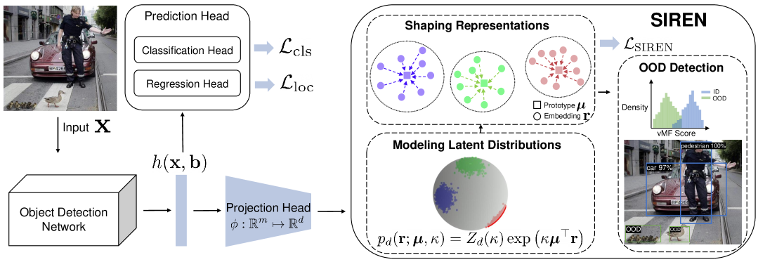
Figure 14: Overview of the proposed learning framework Siren. We introduce a new loss $\mathcal{L}_{\textrm{SIREN}}$ which shapes the representations on the unit hypersphere into compact class-conditional vMF distributions. The embedding $\mathbf{r}\in\mathbb{R}^{d}$ has unit norm $\|\mathbf{r}\|^{2}=1$. In testing, we can employ either parametric or non-parametric distance functions for OOD detection. See Section 15 for details.

15.1 SIREN: Shaping Representations

Modeling the latent distributions.

We propose to model the latent representations by the von Mises-Fisher (vMF) distribution (mardia2000directional), a probability distribution in directional statistics for spherical data with unit norm $\|\mathbf{r}\|^{2}=1$. The probability density function for a unit vector $\mathbf{r}$ in $\mathbb{R}^{d}$ is given as follows:

$$p_{d}(\mathbf{r};\boldsymbol{\mu},\kappa)=Z_{d}(\kappa)\exp\left(\kappa\boldsymbol{\mu}^{\top}\mathbf{r}\right),$$ (23)

where $\kappa\geq 0$, $\|\boldsymbol{\mu}\|^{2}=1$, and the normalization factor $Z_{d}(\kappa)$ is defined as:

$$Z_{d}(\kappa)=\frac{\kappa^{d/2-1}}{(2\pi)^{d/2}I_{d/2-1}(\kappa)},$$ (24)

where $I_{v}$ is the modified Bessel function of the first kind with order $v$. $Z_{d}(\kappa)$ can be calculated in closed form based on $\kappa$ and the dimensionality $d$.  Importantly, the vMF distribution is characterized by two parameters: the mean vector $\boldsymbol{\mu}$ and concentration parameter $\kappa$. Samples that are more aligned with the center $\boldsymbol{\mu}$ have a higher probability density, and vice versa. Here $\kappa$ indicates the tightness of the distribution around the mean direction $\boldsymbol{\mu}$. The larger value of $\kappa$, the stronger the distribution is concentrated in the mean direction. In the extreme case of $\kappa=0$, the sample points are distributed uniformly on the hypersphere.

When considering multiple classes, we can model the embedding space as a mixture of class-conditional vMF distributions, one for each class $c\in\{1,2,...,C\}$:

$$p_{d}^{c}(\mathbf{r};\boldsymbol{\mu}_{c},\kappa_{c})=Z_{d}(\kappa_{c})\exp\left(\kappa_{c}\boldsymbol{\mu}_{c}^{\top}\mathbf{r}\right),$$ (25)

where $\kappa_{c}$ and $\boldsymbol{\mu}_{c}$ are class-conditional parameters. Under this probability model, an embedding vector $\mathbf{r}$ is assigned to class $c$ with the following normalized probability:

$$p(y=c|\mathbf{r};\{\kappa_{j},\boldsymbol{\mu}_{j}\}_{j=1}^{C}) =\frac{Z_{d}\left(\kappa_{c}\right)\exp\left(\kappa_{c}\boldsymbol{\mu}_{c}^{\top}\mathbf{r}\right)}{\sum_{j=1}^{C}Z_{d}\left(\kappa_{j}\right)\exp\left(\kappa_{j}\boldsymbol{\mu}_{j}^{\top}\mathbf{r}\right)}.$$ (26)

Shaping representations.

Our key idea is to design an end-to-end trainable loss function that enables ShapIng the RepresENtations into a mixture of vMF distributions, which facilitates test-time OOD detection in the representation space (Section 15.2). We therefore name our method Siren. The learned mapping function projects an input to a point in the embedding space, where higher probability is assigned to the correct class in comparison to incorrect classes. To achieve this, we can perform maximum likelihood estimation (MLE) on the training data:

$$\text{argmax}_{\theta} \prod_{i=1}^{M}p(y_{i}|\mathbf{r}_{i};\{\kappa_{j},\boldsymbol{\mu}_{j}\}_{j=1}^{C}),$$ (27)

where $i$ is the index of the object embedding and $M$ is the size of the training set. By taking the negative log-likelihood, the objective function is equivalent to minimizing the following loss:

$$\mathcal{L}_{\mathrm{SIREN}}=-\frac{1}{M}\sum_{i=1}^{M}\log\frac{Z_{d}\left(\kappa_{y_{i}}\right)\exp\left(\kappa_{y_{i}}\boldsymbol{\mu}_{y_{i}}^{\top}\mathbf{r}_{i}\right)}{\sum_{j=1}^{C}Z_{d}\left(\kappa_{j}\right)\exp\left(\kappa_{j}\boldsymbol{\mu}_{j}^{\top}\mathbf{r}_{i}\right)},$$ (28)

where $y_{i}$ is the ground truth label for the embedding $\mathbf{r}_{i}$. In effect, $\mathcal{L}_{\mathrm{SIREN}}$ encourages the object embeddings to be aligned with its class prototype, which shapes the representations such that objects in each class form a compact cluster on the hypersphere; see Figure 13 (b).

Prototype estimation and update.

During training, Siren estimates the class-conditional object prototypes $\boldsymbol{\mu}_{c},c\in\{1,2,...,C\}$. The conventional approach for estimating the prototypes is to calculate the mean vector of all training samples (or a subset of them) for each class, and update it periodically during training (DBLP:journals/pr/ZheCY19). Despite its simplicity, this method requires alternating training and prototype estimation, which incurs a heavy computational toll and causes undesirable latency. Instead, we update the class-conditional prototypes in an exponential-moving-average (EMA) manner (DBLP:conf/iclr/0001XH21; DBLP:conf/iclr/WangXLF0CZ22):

$$\boldsymbol{\mu}_{c}:=\text{Normalize}(\alpha\boldsymbol{\mu}_{c}+(1-\alpha)\mathbf{r}),\forall c\in\{1,2,\ldots,C\},$$ (29)

where $\alpha$ is the prototype update factor, and $\mathbf{r}$ denotes the normalized object embeddings from class $c$. The update can be done efficiently with negligible cost, enabling end-to-end training.

Input: ID training data $\mathcal{D}_{\text{tr}}^{\text{in}}=\left\{\left(\mathbf{x}_{i},\mathbf{b}_{i},{y}_{i}\right)\right\}_{i=1}^{M}$, randomly initialized object detector and MLP projection head with parameter $\theta$, loss weight $\beta$ for $\mathcal{L}_{\text{SIREN}}$, and learnable $\{\kappa_{c}\}_{c=1}^{C}$.

Output: Object detector with parameter $\theta^{*}$ and OOD detector $G$.

while train do

    1. Update class-conditional prototypes $\boldsymbol{\mu}_{c}$ with the hyperspherical embeddings $\mathbf{r}$ by Equation (29).

    2. Calculate the vMF-based representation shaping loss $\mathcal{L}_{\textrm{SIREN}}$ by Equation (28).

    3. Update the learnable $\{\kappa_{c}\}_{c=1}^{C}$ and the network parameters $\theta$ using Equation (30).

end while

while eval do

    1. Calculate the OOD score by Equation (31) or Equation (33).

    2. Perform OOD detection by Equation (32).

end while

Algorithm 3 Siren: Shaping Representations for object-level OOD detection

Overall training objective. The overall training objective combines the standard object detection loss, along with our new representation shaping loss $\mathcal{L}_{\textrm{SIREN}}$:

$$\min_{\theta,\kappa}\mathbb{E}_{(\mathbf{x},\mathbf{b},y)\sim\mathcal{P}}\left[\mathcal{L}_{\mathrm{cls}}+\mathcal{L}_{\mathrm{loc}}\right]+\beta\cdot\mathcal{L}_{\textrm{SIREN}},$$ (30)

where $\beta$ is the weight of our representation shaping loss. $\mathcal{L}_{\mathrm{cls}}$ and $\mathcal{L}_{\mathrm{loc}}$ are losses for classification and bounding box regression, respectively. We provide extensive empirical evidence in Section 16 demonstrating the efficacy of our loss function.

To the best of our knowledge, our work makes the first attempt to explore vMF-based learning and inference for object-level OOD detection. To highlight the novelty of the loss itself: we introduce a novel learnable $\{\kappa_{j}\}_{j=1}^{C}$ for each ID class in Equation (28), instead of using fixed values. Our loss allows concentration parameter $\kappa$ to adaptively and flexibly capture the class-conditional feature statistics during training. This is desirable when each ID class may have its own concentration in the hypersphere. We will later show that such learnable $\{\kappa_{j}\}_{j=1}^{C}$ enables better OOD detection performance (Section 30.3).

15.2 Test-time OOD Detection

During inference, we explore and contrast two types of uncertainty scores for detecting OOD objects.

Parametric vMF score. We propose a new test-time OOD score based on the learned class-conditional vMF distributions, parameterized by $\{\widehat{\kappa}_{c},\boldsymbol{\mu}_{c}\}_{c=1}^{C}$. Here $\widehat{\kappa}_{c}$ denotes the learned concentration parameter for class $c$, which captures the concentration of representations for class $c$. For a test-time object $(\mathbf{x}^{\prime},\mathbf{b}^{\prime})$, we use the largest estimated class-conditional likelihood as the OOD score:

$$S\left(\mathbf{x}^{\prime},\mathbf{b}^{\prime}\right)=\max_{c}Z_{d}(\widehat{\kappa}_{c})\exp\left(\widehat{\kappa}_{c}\boldsymbol{\mu}_{c}^{\top}\mathbf{r^{\prime}}\right),$$ (31)

where $\mathbf{r}^{\prime}=\phi(h(\mathbf{x}^{\prime},\mathbf{b}^{\prime}))$ is the normalized embedding from the MLP projection head. Our OOD detection score thus in principle suits our learned embeddings and vMF distributions. For OOD detection, one can use the level set to distinguish between ID and OOD objects:

$$G\left(\mathbf{x}^{\prime},\mathbf{b}^{\prime}\right)=\begin{cases}1&\text{ if }S\left(\mathbf{x}^{\prime},\mathbf{b}^{\prime}\right)\geq\gamma\\ 0&\text{ if }S\left(\mathbf{x}^{\prime},\mathbf{b}^{\prime}\right)<\gamma\end{cases}$$ (32)

The threshold $\gamma$ can be chosen so that a high fraction of ID data (e.g., 95%) is correctly classified. For objects classified as ID, one can obtain the bounding box and class prediction using the prediction head as usual.

Non-parametric KNN score. To relax the distributional assumption on the learned embeddings, we additionally employ a non-parametric KNN distance for OOD detection, which performs well on compact and normalized feature space. Following sun2022out, the KNN distance is defined as:

$$S\left(\mathbf{x}^{\prime},\mathbf{b}^{\prime},k\right)=-\left\|\mathbf{r}^{\prime}-\mathbf{r}_{(k)}\right\|_{2},$$ (33)

where $\mathbf{r}_{(k)}$ denotes the normalized embedding of the $k$-th nearest neighbor (in the training data), for the test embedding $\mathbf{r}^{\prime}$. Our algorithm is summarized in Algorithm 3.

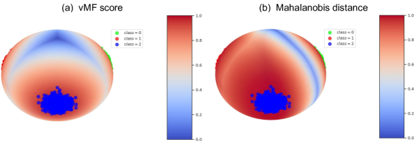
Figure 15: The uncertainty surface is calculated using our vMF score (a) and the Mahalanobis distance (b). We showcase one class for visual clarity.

Remark 1.

Different from Mahalanobis distance (lee2018simple), our parametric vMF-based OOD detection score operates under the same distributional model as the training process, and hence enjoys mathematical compatibility. Computationally, we can directly use the parameters of vMF distributions (such as $\kappa$) learned from training. In contrast, the Mahalanobis distance requires a separate test-time estimation of feature statistics—which involves an expensive and numerically unstable step of calculating the covariance matrix. The distinction of the uncertainty surface calculated by both our vMF score and the Mahalanobis distance is qualitatively demonstrated in Figure 19. The data points are sampled from a mixture of three class-conditional vMF distributions (see details in Appendix 32.6).

16 Experiments

In this section, we validate the effectiveness of Siren on object detection models, including the latest transformer-based (Section 16.1) and flagship CNN-based models (Section 16.2).

Datasets. Following Du et al. (2022c), we use pascal-voc (Everingham et al., 2010) and Berkeley DeepDrive (bdd100k) (DBLP:conf/cvpr/YuCWXCLMD20) datasets as the ID training data. For both tasks, we evaluate on two OOD datasets that contain a subset of images from: ms-coco (lin2014microsoft) and OpenImages (validation set) (kuznetsova2020open). Extensive details on the datasets are in Appendix 32.1.

Metrics. For evaluating the OOD detection performance, we report: (1) the false positive rate (FPR95) of OOD objects when the true positive rate of ID samples is at 95%; (2) the area under the receiver operating characteristic curve (AUROC). For evaluating the object detection performance on the ID task, we report the common metric mAP.

16.1 Evaluation on Transformer-based Model

Experimental details. We adopt a very recent deformable-detr (ddetr) architecture (deformable_detr). ddetr introduces multi-scale deformable attention modules in the transformer encoder and decoder layers of detr (Carion et al., 2020), and provides better convergence and lower complexity. The multi-scale feature maps in ddetr are extracted from a ResNet-50 (He et al., 2016a) pre-trained on ImageNet in a self-supervised fashion, i.e., DINO (Caron et al., 2021). We use the embeddings at the penultimate layer of the decoder in DDETR for projection. For the projection head, we use a two-layer MLP with a ReLU nonlinearity, with dimensionality $256\rightarrow d\rightarrow d$. The dimension $d$ of the unit hypersphere is 16 for pascal-voc and 64 for bdd100k. The default weight $\beta$ for the Siren is 1.5 and the prototype update factor $\alpha$ is 0.95. We initialize the learnable $\kappa$ to be 10 for all classes. The $k$ in the KNN distance is set to 10. Ablations on the hyperparameters are provided in Section 30.3 and Appendix 32.3. Other hyperparameters are the same as the default ones in ddetr (deformable_detr).

In-distribution dataset	Method	FPR95 $\downarrow$	AUROC $\uparrow$	mAP (ID)$\uparrow$
		OOD: MS-COCO / OpenImages
PASCAL-VOC	Mahalanobis (lee2018simple)	97.39 / 97.88	50.28 / 49.08	60.6
	Gram matrices (DBLP:conf/icml/SastryO20)	94.16 / 95.29	43.97 / 38.81	60.6
	KNN (sun2022out)	91.80 / 91.36	62.15 / 59.64	60.6
	CSI (tack2020csi)	84.00 / 79.16	55.07 / 51.37	59.5
	VOS (Du et al., 2022c)	97.46 / 97.07	54.40 / 52.77	60.3
	OW-DETR (Gupta et al., 2022)	93.09 / 93.82	55.70 / 57.80	58.3
	Dismax (dismax)	82.05 / 76.37	75.21 / 70.66	60.1
	Siren-vMF (ours)	75.49$\pm$0.8 / 78.36$\pm$1.0	76.10$\pm$0.1 / 71.05$\pm$0.1	60.8$\pm$0.1
	Siren-KNN (ours)	64.77$\pm$0.2 / 65.99$\pm$0.5	78.23$\pm$0.2 / 74.93$\pm$0.1	60.8$\pm$0.1
	Siren-vMF (rerun)	76.52 / 79.23	76.22 / 71.19	60.8
	Siren-KNN (rerun)	64.64 / 65.48	78.72 / 75.43	60.8
BDD100K	Mahalanobis (lee2018simple)	70.86 / 71.43	76.83 / 77.98	31.3
	Gram matrices (DBLP:conf/icml/SastryO20)	73.81 / 71.56	60.13 / 57.14	31.3
	KNN (sun2022out)	64.75 / 61.13	80.90 / 79.64	31.3
	CSI (tack2020csi)	70.27 / 71.30	77.93 / 76.42	29.9
	VOS (Du et al., 2022c)	76.44 / 72.58	77.33 / 76.62	31.0
	OW-DETR (Gupta et al., 2022)	80.78 / 77.37	70.29 / 73.78	28.1
	Dismax (dismax)	77.62 / 81.23	72.14 / 67.18	31.2
	Siren-vMF (ours)	67.54$\pm$1.3 / 66.31$\pm$0.9	80.06$\pm$0.5 / 79.77$\pm$1.2	31.3$\pm$0.0
	Siren-KNN (ours)	53.97$\pm$0.7 / 47.28$\pm$0.3	86.56$\pm$0.1 / 89.00$\pm$0.4	31.3$\pm$0.0
	Siren-vMF (rerun)	68.79 / 69.86	79.14 / 77.35	31.3
	Siren-KNN (rerun)	55.75 / 50.40	85.89 / 88.26	31.3

Table 9: Main results. Comparison with competitive out-of-distribution detection methods. All baseline methods are based on the same model backbone ddetr. $\uparrow$ indicates larger values are better and $\downarrow$ indicates smaller values are better. All values are percentages. Bold numbers are superior results. We report standard deviations estimated across 3 runs. Siren-vMF/KNN denotes using vMF score and KNN distance during inference.

Siren achieves superior performance.

In Table 9, we compare Siren with competitive OOD detection methods in literature. For a fair comparison, all the methods only use ID data for training. Siren outperforms competitive baselines, including Mahalanobis distance (lee2018simple), KNN distance (sun2022out), CSI (tack2020csi), Gram matrices (DBLP:conf/icml/SastryO20) and Dismax (dismax). These baselines operate on feature embedding space, allowing a fair comparison. Note that other common output-based methods (such as MSP (Hendrycks and Gimpel, 2017), ODIN (liang2018enhancing), and energy (liu2020energy)) are not directly applicable for multi-label classification networks in ddetr. For these methods relying on a multi-class classification model, we will later provide comparisons on the Faster R-CNN model in Section 16.2. Implementation details and the training time for all the baseline methods are reported in Appendix 32.4 and 32.5. We highlight a few observations:

1) The comparison between SIREN vs. Mahalanobis highlights precisely the benefits of our embedding shaping loss $\mathcal{L}_{\text{SIREN}}$. As shown in Figure 13, the vanilla detr model produces ill-conditioned embeddings that do not conform to multivariate Gaussian distributions, rendering the Mahalanobis approach ineffective (with AUROC around 50%–which is random guessing). In contrast, Siren-vMF improves the OOD detection performance (AUROC) by 25.82% on pascal-voc (ms-coco as OOD). Different from the Mahalanobis distance, our parametric vMF scoring function naturally suits the learned hyperspherical embeddings with vMF distributions. The advantage of the vMF loss can be further verified by observing that Siren-KNN outperforms directly applying KNN distance on the vanilla ddetr (16.08% AUROC improvement on voc with coco as OOD).

2) Siren outperforms the latest methods VOS (Du et al., 2022c) and OW-DETR (Gupta et al., 2022), which are designed for object detection models and serve as strong baselines for us. Compared with OW-DETR, Siren-KNN substantially improves the AUROC by 22.53% on pascal-voc (coco as OOD). OW-DETR uses the unmatched object queries with high confidence as the unknowns, and trains a binary classifier to separate ID and unknown objects. However, the unmatched object queries might be distributionally too close to the ID classes and thus displays limited improvement for OOD detection. In addition, VOS synthesizes virtual outliers from the class-conditional Gaussian distributions of the penultimate layer but fails to perform well due to the ill-conditioned embedding distribution in ddetr (non-Gaussian).

16.2 Evaluation on CNN-based Model

Method	FPR95 $\downarrow$	AUROC $\uparrow$	Time
	COCO/ OpenImages
MSP	70.99 / 73.13	83.45 / 81.91	2.1 h
ODIN	59.82 / 63.14	82.20 / 82.59	2.1 h
Mahalanobis	96.46 / 96.27	59.25 / 57.42	2.1 h
Energy score	56.89 / 58.69	83.69 / 82.98	2.1 h
Gram matrices	62.75 / 67.42	79.88 / 77.62	2.1 h
KNN	52.67 / 53.67	87.14 / 84.54	2.1 h
CSI	59.91 / 57.41	81.83 / 82.95	4.9 h
GAN-synthesis	60.93 / 59.97	83.67 / 82.67	3.7 h
VOS	47.53 / 51.33	88.70 / 85.23	4.3 h
Dismax	84.38 / 86.93	74.56 / 71.53	2.2 h
Siren-vMF (ours)	64.68 / 68.53	85.36 / 82.78	2.1 h
Siren-KNN (ours)	47.45 / 50.38	89.67 / 88.80	2.1 h

Table 10: OOD detection results of Siren and comparison with competitive baselines on two OOD datasets: COCO and OpenImages.

Going beyond detection transformers, we show that Siren is also suitable and effective on CNN-based object-level OOD detection models, e.g., Faster R-CNN (ren2015faster). Table 10 showcases the OOD detection performance with Siren trained on pascal-voc dataset and evaluated on both ms-coco and OpenImages datasets. In addition to baselines considered in Table 9, we include common output-based methods relying on multi-class classification, such as MSP, ODIN, and energy score.

In Table 10, we additionally report training time comparison. Siren consistently improves OOD detection performance on both OOD datasets. Notably, Siren performs better than the previous best OOD detection approach VOS on Faster R-CNN while preserving the same training time as vanilla Faster R-CNN.

17 Ablations and Discussions

In this section, we provide ablation results on how different factors impact the performance of Siren. For consistency, we present the analyses below based on the ddetr model. Unless otherwise pointed, we use the KNN distance by default.

Ablations on learnable vs. fixed $\kappa$. In this ablation, we show that our approach using learnable concentration parameters $\{\kappa_{c}\}_{c=1}^{C}$ is better than using the fixed ones. Our method with learnable $\kappa$ is desirable, since each ID class may have its own concentration in the hypersphere. With fixed $\kappa$, the loss function can be simplified as follows:

$$\mathcal{L}=-\frac{1}{M}\sum_{i=1}^{M}\log\frac{\exp\left(\kappa\boldsymbol{\mu}_{y_{i}}^{\top}\mathbf{r}_{i}\right)}{\sum_{j=1}^{C}\exp\left(\kappa\boldsymbol{\mu}_{j}^{\top}\mathbf{r}_{i}\right)}.$$ (34)

Empirically, we indeed observe that employing learnable $\{\kappa_{c}\}_{c=1}^{C}$ achieves better OOD detection performance, with AUROC 78.23% on pascal-voc model (ms-coco as OOD). In Figure 16 (a), we show Siren’s performance when trained under different fixed $\kappa$ values. The best model under the fixed $\kappa=10$ achieves an AUROC of 77.67%. Too small of $\kappa$ value (e.g., $\kappa=1$) leads to almost uniform distributions and is therefore not desirable.

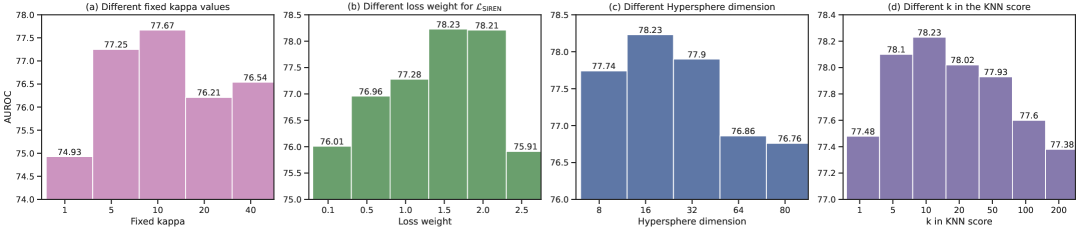
Figure 16: (a) Ablation study on using different fixed values of concentration parameter $\kappa$ in Equation (34). (b) Ablation on different weights $\beta$ for $\mathcal{L}_{\textrm{SIREN}}$ in Equation (30). (c) Ablation on the dimension of the hyperspherical embeddings $\mathbf{r}$. (d) Ablation study on the parameter $k$ in the KNN-based OOD detection score for Siren. Numbers are AUROC. The ID training dataset is pascal-voc and OOD dataset is ms-coco.

Ablations on the Siren loss weight $\beta$.

Figure 16 (b) reports the OOD detection results as we vary the weight $\beta$ for the representation shaping loss $\mathcal{L}_{\textrm{SIREN}}$. The model is evaluated on the ms-coco dataset as OOD. Overall a mild weight works well. Across all the $\beta$ values considered, Siren consistently outperforms the baseline OOD detection methods in Table 9. One can use our Siren loss as an easy plug-in module, with minimal hyperparameter tuning.

Ablations on the dimension $d$ of hypersphere.

Siren projects the object feature embeddings into a lower-dimensional hypersphere in $\mathbb{R}^{d}$, which allows tractable vMF estimation. Figure 16 (c) shows the effect the embedding dimension $d$ on the OOD detection performance. We find that a lower dimension between 16 and 64 achieves favorable and stable performance. In the extreme case with dimension $d=8$, the model suffers from considerable information loss and degraded performance. On the other hand, too large of $d$ causes training instability, which is not desirable either.

Ablations on the uncertainty score. We perform ablation on two variants of the vMF-based OOD detection score (c.f. Equation (31)): using the learned $\{\kappa_{c}\}_{c=1}^{C}$ vs. approximately estimate the $\kappa$ parameters directly from the converged embeddings. In literature, there are several established methods for approximating $\kappa$ (mardia2000directional). Denote $\mathbf{\overline{r}}_{c}$ the average of object embeddings for class $c$, the simplest approximate solution is given as follows:

$$\widehat{\kappa_{c}}=\frac{\|\mathbf{\overline{r}}_{c}\|(d-\|\mathbf{\overline{r}}_{c}\|^{2})}{1-\|\mathbf{\overline{r}}_{c}\|^{2}},$$ (35)

The proof is given in Appendix 32.2. We show in Table 11 that using learned $\{\kappa_{c}\}_{c=1}^{C}$ avoids the imprecision in approximating $\widehat{\kappa_{c}}$ directly from embeddings. This affirms the importance of employing learnable concentration parameters in our Siren loss. Moreover, the non-parametric KNN density estimation provides stronger flexibility and generality, and leads to better performance.

	FPR95 $\downarrow$	AUROC $\uparrow$
	COCO / OpenImages as OOD
vMF w/ $\kappa$ from (DBLP:journals/cstat/Sra12)	78.60 / 78.42	73.03 / 70.27
vMF w/ learned $\kappa$ (ours)	75.49 / 78.36	76.10 / 71.05
Non-parametric KNN distance	64.77 / 65.99	78.23 / 74.93

Table 11: Ablation on different OOD detection scores. The ID dataset is pascal-voc.

Ablations on the projection head.

We ablate on the nonlinearity in the projection head by comparing with Siren trained with a linear layer in Table 12. The result shows using a nonlinear mapping for projection helps obtain a more expressive hypersphere, which improves OOD detection by 4.37% in terms of AUROC (ms-coco as OOD, vMF as the OOD score).

	FPR95 $\downarrow$	AUROC $\uparrow$
	COCO / OpenImages as OOD
vMF w/o nonlinearity	82.85 / 83.69	71.73 / 66.82
vMF w/ nonlinearity	75.49 / 78.36	76.10 / 71.05
1-3[1pt/1pt] KNN w/o nonlinearity	67.03 / 72.11	78.02 / 72.42
KNN w/ nonlinearity	64.77 / 65.99	78.23 / 74.93

Table 12: Ablation on the projection head. The ID dataset is pascal-voc.

18 Qualitative analysis

In Figure 17, we visualize the predictions on several OOD images, using object detection models trained without Siren (top) and with Siren (bottom), respectively. The in-distribution data is bdd100k. Siren better identifies OOD objects (in green) compared to a vanilla object detector ddetr, reducing false positives. Moreover, the confidence score of the false-positive objects of Siren is lower than that of the vanilla model (see the train/bicycle in the 3rd/5th column).

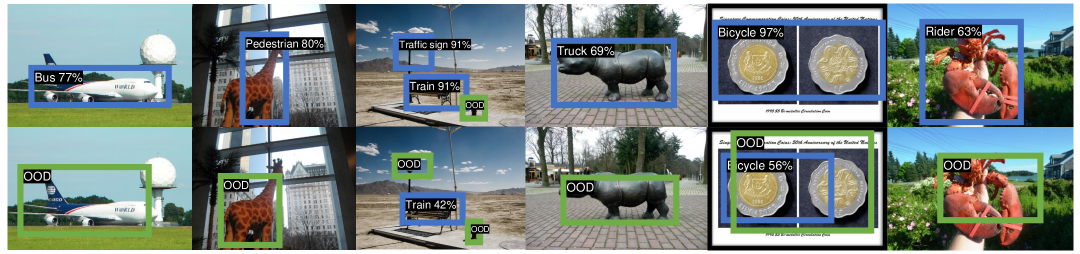
Figure 17: Visualization of detected objects on the OOD images (from ms-coco and OpenImages) by vanilla ddetr (top) and Siren (bottom). The ID is bdd100k dataset. Blue: OOD objects classified as the ID classes. Green: OOD objects detected by ddetr and Siren, which reduce false positives.

19 Summary

In this chapter, we propose a novel framework Siren, which tackles object-level OOD detection with a distance-based approach. Siren mitigates the key shortcoming of the previous output-based OOD detection approach, and explores a new vMF loss to shape representations for OOD detection. To the best of our knowledge, Siren makes the first attempt to employ vMF-based learning and inference for OOD detection. Siren establishes competitive performance on challenging object-level OOD detection tasks, evaluated broadly under both the recent detection transformers and CNN-based models. Our in-depth ablations provide further insights on the efficacy of Siren. We hope our work inspires future research on OOD detection with representation shaping.

Chapter 7 Overview for Learning in the Wild with Unlabeled Data

Motivation. Previous research utilizing auxiliary outlier datasets has shown promise in improving OOD detection compared to models trained solely on ID data. These models often regularize confidence scores (Hendrycks et al., 2019) or energy levels (liu2020energy) for outlier data. However, this approach faces two significant limitations: (1) auxiliary data collected offline may not accurately reflect the true distribution of unknown data encountered in real-world settings, potentially undermining OOD detection during deployment; (2) collecting such data is often labor-intensive and requires careful cleaning to avoid overlap with ID data.

My research addresses these challenges by building novel learning algorithms and theories that leverage unlabeled "in-the-wild" data, which can be gathered at minimal cost during the deployment of machine learning models. This type of data has been largely overlooked in OOD learning contexts. Formally, unlabeled data can be represented by a Huber contamination model, $\mathbb{P}_{\text{unlabeled}}:=(1-\pi)\mathbb{P}_{\text{in}}+\pi\mathbb{P}_{\text{out}}$, where $\mathbb{P}_{\text{in}}$ and $\mathbb{P}_{\text{out}}$ represent the marginal distributions of ID and OOD data, respectively. Unlabeled data is abundant, does not require human annotation, and often better aligns with true test-time distributions compared to offline-collected data. While this setting is promising for various applications, it introduces unique challenges due to the impure nature of the unlabeled data which comprises both ID and OOD samples.

Theoretical foundations of learning with wild data. In my ICLR’24 paper SAL (Du et al., 2024a), I conducted the first formal investigation on when and how unlabeled data can enhance OOD detection. My contributions are: (1) I proposed a novel learning framework that separates candidate outliers using singular value decomposition on the model gradient matrix, which facilitates the learning of an OOD classifier. (2) The framework provides theoretical support for the filtering error and the generalization error of the OOD classifier, proving that these errors can be small under specific conditions. (3) Empirically, I demonstrated the generalization bounds of SAL translate into strong empirical performance, establishing state-of-the-art results through extensive evaluations. Particularly, Chapter 8 is going to mainly discuss the work of SAL.

Learning with diverse data shifts in the wild. Beyond detecting samples with semantic shifts, machine learning models may also encounter covariate shifts—variations in input distributions that do not necessarily affect labels. These shifts can arise from differences in sensor calibration or environmental changes. My ICML’23 paper, SCONE (Bai et al., 2023a), along with a recent preprint (Bai et al., 2024) were the first to explore techniques for modeling diverse mixtures of data shifts, expressed as $\mathbb{P}_{\text{unlabeled}}:=(1-\pi_{c}-\pi_{s})\mathbb{P}_{\text{in}}+\pi_{c}\mathbb{P}_{\text{out}}^{\text{covariate}}+\pi_{s}\mathbb{P}_{\text{out}}^{\text{semantic}}$. This framework integrates ID data and various OOD distributions, and employs constrained optimization and active learning to effectively learn with these diverse data sources for both OOD detection and OOD generalization. The formulation and methodologies presented offer strong generality and practicality for real-world applications.

Chapter 8 How Does Unlabeled Data Provably Help Out-of-Distribution Detection?

Publication Statement. This chapter is joint work with Zhen Fang, Ilias Diakonikolas and Yixuan Li. The paper version of this chapter appeared in ICLR’24 (Du et al., 2024a).

Abstract. Using unlabeled data to regularize the machine learning models has demonstrated promise for improving safety and reliability in detecting out-of-distribution (OOD) data. Harnessing the power of unlabeled in-the-wild data is non-trivial due to the heterogeneity of both in-distribution (ID) and OOD data. This lack of a clean set of OOD samples poses significant challenges in learning an optimal OOD classifier. Currently, there is a lack of research on formally understanding how unlabeled data helps OOD detection. This chapter bridges the gap by introducing a new learning framework SAL (Separate And Learn) that offers both strong theoretical guarantees and empirical effectiveness. The framework separates candidate outliers from the unlabeled data and then trains an OOD classifier using the candidate outliers and the labeled ID data. Theoretically, we provide rigorous error bounds from the lens of separability and learnability, formally justifying the two components in our algorithm. Our theory shows that SAL can separate the candidate outliers with small error rates, which leads to a generalization guarantee for the learned OOD classifier. Empirically, SAL achieves state-of-the-art performance on common benchmarks, reinforcing our theoretical insights. Code is publicly available at https://github.com/deeplearning-wisc/sal.

20 Introduction

When deploying machine learning models in real-world environments, their safety and reliability are often challenged by the occurrence of out-of-distribution (OOD) data, which arise from unknown categories and should not be predicted by the model. Concerningly, neural networks are brittle and lack the necessary awareness of OOD data in the wild (nguyen2015deep). Identifying OOD inputs is a vital but fundamentally challenging problem—the models are not explicitly exposed to the unknown distribution during training, and therefore cannot capture a reliable boundary between in-distribution (ID) vs. OOD data. To circumvent the challenge, researchers have started to explore training with additional data, which can facilitate a conservative and safe decision boundary against OOD data. In particular, a recent work by Katz-Samuels et al. (2022) proposed to leverage unlabeled data in the wild to regularize model training, while learning to classify labeled ID data. Such unlabeled wild data offer the benefits of being freely collectible upon deploying any machine learning model in its operating environment, and allow capturing the true test-time OOD distribution.

Despite the promise, harnessing the power of unlabeled wild data is non-trivial due to the heterogeneous mixture of ID and OOD data. This lack of a clean set of OOD training data poses significant challenges in designing effective OOD learning algorithms. Formally, the unlabeled data can be characterized by a Huber contamination model $\mathbb{P}_{\text{wild}}:=(1-\pi)\mathbb{P}_{\text{in}}+\pi\mathbb{P}_{\text{out}}$, where $\mathbb{P}_{\text{in}}$ and $\mathbb{P}_{\text{out}}$ are the marginal distributions of the ID and OOD data. It is important to note that the learner only observes samples drawn from such mixture distributions, without knowing the clear membership of whether being ID or OOD. Currently, a formalized understanding of the problem is lacking for the field. This prompts the question underlying the present work:

Algorithmic contribution. In this chapter, we propose a new learning framework SAL (Separate And Learn), that effectively exploits the unlabeled wild data for OOD detection. At a high level, our framework SAL builds on two consecutive components: (1) filtering—separate candidate outliers from the unlabeled data, and (2) classification—learn an OOD classifier with the candidate outliers, in conjunction with the labeled ID data. To separate the candidate outliers, our key idea is to perform singular value decomposition on a gradient matrix, defined over all the unlabeled data whose gradients are computed based on a classification model trained on the clean labeled ID data. In the SAL framework, unlabeled wild data are considered candidate outliers when their projection onto the top singular vector exceeds a given threshold. The filtering strategy for identifying candidate outliers is theoretically supported by Theorem 8.1. We show in Section 21 (Remark 1) that under proper conditions, with a high probability, there exist some specific directions (e.g., the top singular vector direction) where the mean magnitude of the gradients for the wild outlier data is larger than that of ID data. After obtaining the outliers from the wild data, we train an OOD classifier that optimizes the classification between the ID vs. candidate outlier data for OOD detection.

Theoretical significance. Importantly, we provide new theories from the lens of separability and learnability, formally justifying the two components in our algorithm. Our main Theorem 8.1 analyzes the separability of outliers from unlabeled wild data using our filtering procedure, and gives a rigorous bound on the error rate. Our theory has practical implications. For example, when the size of the labeled ID data and unlabeled data is sufficiently large, Theorems 8.1 and 8.2 imply that the error rates of filtering outliers can be bounded by a small bias proportional to the optimal ID risk, which is a small value close to zero in reality (Frei et al., 2022). Based on the error rate estimation, we give a generalization error of the OOD classifier in Theorem 8.3, to quantify its learnability on the ID data and a noisy set of candidate outliers. Under proper conditions, the generalization error of the learned OOD classifier is upper bounded by the risk associated with the optimal OOD classifier.

Empirical validation. Empirically, we show that the generalization bound w.r.t. SAL (Theorem 8.3) indeed translates into strong empirical performance. SAL can be broadly applicable to non-convex models such as modern neural networks. We extensively evaluate SAL on common OOD detection tasks and establish state-of-the-art performance. For completeness, we compare SAL with two families of methods: (1) trained with only $\mathbb{P}_{\text{in}}$, and (2) trained with both $\mathbb{P}_{\text{in}}$ and an unlabeled dataset. On Cifar-100, compared to a strong baseline KNN+ (sun2022out) using only $\mathbb{P}_{\text{in}}$, SAL outperforms by 44.52% (FPR95) on average. While methods such as Outlier Exposure (Hendrycks et al., 2019) require a clean set of auxiliary unlabeled data, our results are achieved without imposing any such assumption on the unlabeled data and hence offer stronger flexibility. Compared to the most related baseline WOODS (Katz-Samuels et al., 2022), our framework can reduce the FPR95 from 7.80% to 1.88% on Cifar-100, establishing near-perfect results on this challenging benchmark.

21 Proposed Methodology

In this section, we introduce a new learning framework SAL that performs OOD detection by leveraging the unlabeled wild data. The framework offers substantial advantages over the counterpart approaches that rely only on the ID data, and naturally suits many applications where machine learning models are deployed in the open world. SAL has two integral components: (1) filtering—separate the candidate outlier data from the unlabeled wild data (Section 21.1), and (2) classification—train a binary OOD classifier with the ID data and candidate outliers (Section 21.2). In Section 22, we provide theoretical guarantees for SAL, provably justifying the two components in our method.

21.1 Separating Candidate Outliers from the Wild Data

To separate candidate outliers from the wild mixture $\mathcal{S}_{\text{wild}}$, our framework employs a level-set estimation based on the gradient information. The gradients are estimated from a classification predictor $\mathbf{h}_{\mathbf{w}}$ trained on the ID data $\mathcal{S}^{\text{in}}$. We describe the procedure formally below.

Estimating the reference gradient from ID data. To begin with, SAL estimates the reference gradients by training a classifier $\mathbf{h}_{\mathbf{w}}$ on the ID data $\mathcal{S}^{\text{in}}$ by empirical risk minimization (ERM):

$$\mathbf{w}_{\mathcal{S}^{\text{in}}}\in\operatorname*{arg\,min}_{\mathbf{w}\in\mathcal{W}}R_{\mathcal{S}^{\text{in}}}(\mathbf{h}_{\mathbf{w}}),~~\text{where}~~R_{\mathcal{S}^{\text{in}}}(\mathbf{h}_{\mathbf{w}})=\frac{1}{n}\sum_{(\mathbf{x}_{i},y_{i})\in\mathcal{S}^{\text{in}}}\ell(\mathbf{h}_{\mathbf{w}}(\mathbf{x}_{i}),y_{i}),$$ (36)

$\mathbf{w}_{\mathcal{S}^{\text{in}}}$ is the learned parameter and $n$ is the size of ID training set $\mathcal{S}^{\text{in}}$. The average gradient $\bar{\nabla}$ is

$$\bar{\nabla}=\frac{1}{n}\sum_{(\mathbf{x}_{i},y_{i})\in\mathcal{S}^{\text{in}}}\nabla\ell(\mathbf{h}_{\mathbf{w}_{\mathcal{S}^{\text{in}}}}(\mathbf{x}_{i}),y_{i}),$$ (37)

where $\bar{\nabla}$ acts as a reference gradient that allows measuring the deviation of any other points from it.

Separate candidate outliers from the unlabeled wild data. After training the classification predictor on the labeled ID data, we deploy the trained predictor $\mathbf{h}_{\mathbf{w}_{\mathcal{S}^{\text{in}}}}$ in the wild, and naturally receives data $\mathcal{S}_{\text{wild}}$—a mixture of unlabeled ID and OOD data. Key to our framework, we perform a filtering procedure on the wild data $\mathcal{S}_{\text{wild}}$, identifying candidate outliers based on a filtering score. To define the filtering score, we represent each point in $\mathcal{S}_{\text{wild}}$ as a gradient vector, relative to the reference gradient $\bar{\nabla}$. Specifically, we calculate the gradient matrix (after subtracting the reference gradient $\bar{\nabla}$) for the wild data as follows:

$$\mathbf{G}=\left[\begin{array}[]{c}\nabla\ell(\mathbf{h}_{\mathbf{w}_{\mathcal{S}^{\text{in}}}}(\tilde{\mathbf{x}}_{1}),\widehat{y}_{\tilde{\mathbf{x}}_{1}})-\bar{\nabla}\\ ...\\ \nabla\ell(\mathbf{h}_{\mathbf{w}_{\mathcal{S}^{\text{in}}}}(\tilde{\mathbf{x}}_{m}),\widehat{y}_{\tilde{\mathbf{x}}_{m}})-\bar{\nabla}\end{array}\right]^{\top},$$ (38)

where $m$ denotes the size of the wild data, and $\widehat{y}_{\tilde{\mathbf{x}}}$ is the predicted label for a wild sample $\tilde{\mathbf{x}}$. For each data point $\tilde{\mathbf{x}}_{i}$ in $\mathcal{S}_{\text{wild}}$, we then define our filtering score as follows:

$$\tau_{i}=\left<\nabla\ell(\mathbf{h}_{\mathbf{w}_{\mathcal{S}^{\text{in}}}}\big{(}\tilde{\mathbf{x}}_{i}),\widehat{y}_{\tilde{\mathbf{x}}_{i}})-\bar{\nabla},\mathbf{v}\right>^{2},$$ (39)

where $\left<\cdot,\cdot\right>$ is the dot product operator and $\mathbf{v}$ is the top singular vector of $\mathbf{G}$. The top singular vector $\mathbf{v}$ can be regarded as the principal component of the matrix $\mathbf{G}$ in Eq. 38, which maximizes the total distance from the projected gradients (onto the direction of $\mathbf{v}$) to the origin (sum over all points in $\mathcal{S}_{\text{wild}}$) (Hotelling, 1933). Specifically, $\mathbf{v}$ is a unit-norm vector and can be computed as follows:

$$\vskip-1.00006pt\mathbf{v}\in\operatorname*{arg\,max}_{\|\mathbf{u}\|_{2}=1}\sum_{\tilde{\mathbf{x}}_{i}\in\mathcal{S}_{\text{wild}}}\left<\mathbf{u},\nabla\ell(\mathbf{h}_{\mathbf{w}_{\mathcal{S}^{\text{in}}}}\big{(}\tilde{\mathbf{x}}_{i}),\widehat{y}_{\tilde{\mathbf{x}}_{i}})-\bar{\nabla}\right>^{2}.$$ (40)

Essentially, the filtering score $\tau_{i}$ in Eq. 39 measures the $\ell_{2}$ norm of the projected vector. To help readers better understand our design rationale, we provide an illustrative example of the gradient vectors and their projections in Figure 18 (see caption for details). Theoretically, Remark 1 below shows that the projection of the OOD gradient vector to the top singular vector of the gradient matrix $\mathbf{G}$ is on average provably larger than that of the ID gradient vector, which rigorously justifies our idea of using the score $\tau$ for separating the ID and OOD data.

Remark 1.

Theorem 4 in Appendix 33.9 has shown that under proper assumptions, if we have sufficient data and large-size model, then with the high probability:

• the mean projected magnitude of OOD gradients in the direction of the top singular vector of $\mathbf{G}$ can be lower bounded by a positive constant $C/\pi$;

• the mean projected magnitude of ID gradients in the direction of the top singular vector is upper bounded by a small value close to zero.

Finally, we regard $\mathcal{S}_{T}=\{\tilde{\mathbf{x}}_{i}\in\mathcal{S}_{\text{wild}}:\mathbf{\tau}_{i}>T\}$ as the (potentially noisy) candidate outlier set, where $T$ is the filtering threshold. The threshold can be chosen on the ID data $\mathcal{S}^{\text{in}}$ so that a high fraction (e.g., 95%) of ID samples is below it. In Section 22, we will provide formal guarantees, rigorously justifying that the set $\mathcal{S}_{T}$ returns outliers with a large probability. We discuss and compare with alternative gradient-based scores (e.g., GradNorm (Huang et al., 2021)) for filtering in Section 23.2. In Appendix 33.23, we discuss the variants of using multiple singular vectors, which yield similar results.

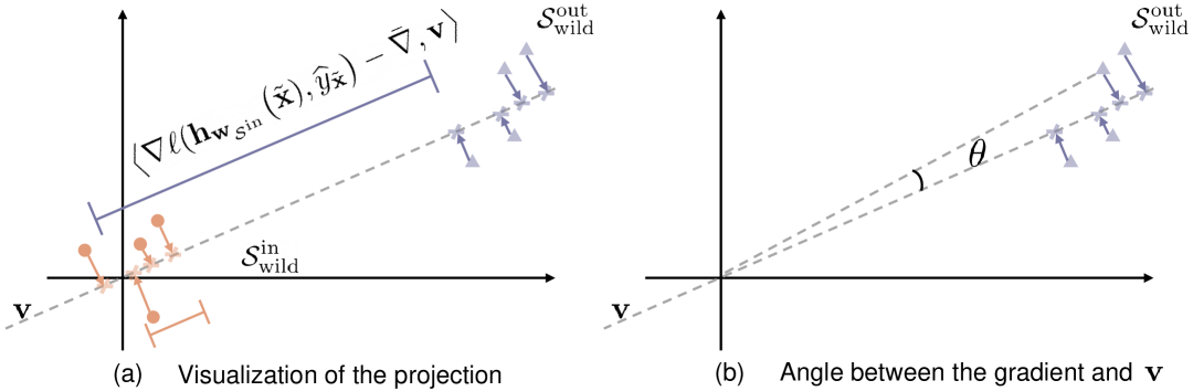
Figure 18: (a) Visualization of the gradient vectors, and their projection onto the top singular vector $\mathbf{v}$ (in gray dashed line). The gradients of inliers from $\mathcal{S}_{\text{wild}}^{\text{in}}$ (colored in orange) are close to the origin (reference gradient $\bar{\nabla}$). In contrast, the gradients of outliers from $\mathcal{S}_{\text{wild}}^{\text{out}}$ (colored in purple) are farther away. (b) The angle $\theta$ between the gradient of set $\mathcal{S}_{\text{wild}}^{\text{out}}$ and the singular vector $\mathbf{v}$. Since $\mathbf{v}$ is searched to maximize the distance from the projected points (cross marks) to the origin (sum over all the gradients in $\mathcal{S}_{\text{wild}}$), $\mathbf{v}$ points to the direction of OOD data in the wild with a small $\theta$. This further translates into a high filtering score $\tau$, which is essentially the norm after projecting a gradient vector onto $\mathbf{v}$. As a result, filtering outliers by $\mathcal{S}_{T}=\{\tilde{\mathbf{x}}_{i}\in\mathcal{S}_{\text{wild}}:\mathbf{\tau}_{i}>T\}$ will approximately return the purple OOD samples in the wild data.

An illustrative example of algorithm effect. To see the effectiveness of our filtering score, we test on two simulations in Figure 19 (a). These simulations are constructed with simplicity in mind, to facilitate understanding. Evaluations on complex high-dimensional data will be provided in Section 23. In particular, the wild data is a mixture of ID (multivariate Gaussian with three classes) and OOD. We consider two scenarios of OOD distribution, with ground truth colored in purple. Figure 19 (b) exemplifies the outliers (in green) identified using our proposed method, which largely aligns with the ground truth. The error rate of $\mathcal{S}_{T}$ containing ID data is only $8.4\%$ and $6.4\%$ for the two scenarios considered. Moreover, the filtering score distribution displays a clear separation between the ID vs. OOD parts, as evidenced in Figure 19 (c).

Remark 2. Our filtering process can be easily extended into $K$-class classification. In this case, one can maintain a class-conditional reference gradient $\bar{\nabla}_{k}$, one for each class $k\in[1,K]$, estimated on ID data belonging to class $k$, which captures the characteristics for each ID class. Similarly, the top singular vector computation can also be performed in a class-conditional manner, where we replace the gradient matrix with the class-conditional $\mathbf{G}_{k}$, containing gradient vectors of wild samples being predicted as class $k$.

21.2 Training the OOD Classifier with the Candidate Outliers

After obtaining the candidate outlier set $\mathcal{S}_{T}$ from the wild data, we train an OOD classifier $\mathbf{g}_{\boldsymbol{\theta}}$ that optimizes for the separability between the ID vs. candidate outlier data. In particular, our training objective can be viewed as explicitly optimizing the level-set based on the model output (threshold at 0), where the labeled ID data $\mathbf{x}$ from $\mathcal{S}^{\text{in}}$ has positive values and vice versa.

$$\begin{split}R_{\mathcal{S}^{\text{in}},\mathcal{S}_{T}}(\mathbf{g}_{\boldsymbol{\theta}})&=R_{\mathcal{S}^{\text{in}}}^{+}(\mathbf{g}_{\boldsymbol{\theta}})+R_{\mathcal{S}_{T}}^{-}(\mathbf{g}_{\boldsymbol{\theta}})\\ &=\mathbb{E}_{\mathbf{x}\in\mathcal{S}^{\text{in}}}~~\mathds{1}\{\mathbf{g}_{\boldsymbol{\theta}}(\mathbf{x})\leq 0\}+\mathbb{E}_{\tilde{\mathbf{x}}\in\mathcal{S}_{T}}~~\mathds{1}\{\mathbf{g}_{\boldsymbol{\theta}}(\tilde{\mathbf{x}})>0\}.\end{split}$$ (41)

To make the $0/1$ loss tractable, we replace it with the binary sigmoid loss, a smooth approximation of the $0/1$ loss. We train $\mathbf{g}_{\boldsymbol{\theta}}$ along with the ID risk in Eq. 36 to ensure ID accuracy. Notably, the training enables strong generalization performance for test OOD samples drawn from $\mathbb{P}_{\text{out}}$. We provide formal guarantees on the generalization bound in Theorem 8.3, as well as empirical support in Section 23. A pseudo algorithm of SAL is in Appendix (see Algorithm 1).

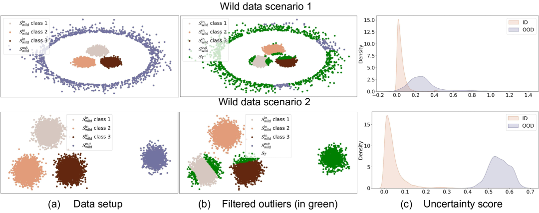
Figure 19: Example of SAL on two different scenarios of the unlabeled wild data. (a) Setup of the ID/inlier $\mathcal{S}_{\text{wild}}^{\text{in}}$ and OOD/outlier data $\mathcal{S}_{\text{wild}}^{\text{out}}$ in the wild. The inliers are sampled from three multivariate Gaussians. We construct two different distributions of outliers (see details in Appendix 33.29). (b) The filtered outliers (in green) by SAL, where the error rate of filtered outliers $\mathcal{S}_{T}$ containing inlier data is $8.4\%$ and $6.4\%$, respectively. (c) The density distribution of the filtering score $\tau$, which is separable for inlier and outlier data in the wild and thus benefits the training of the OOD classifier leveraging the filtered outlier data for binary classification.

22 Theoretical Analysis

We now provide theory to support our proposed algorithm. Our main theorems justify the two components in our algorithm. As an overview, Theorem 8.1 provides a provable bound on the error rates using our filtering procedure. Based on the estimations on error rates, Theorem 8.3 gives the generalization bound w.r.t. the empirical OOD classifier $\mathbf{g}_{\boldsymbol{\theta}}$, learned on ID data and noisy set of outliers. We specify several mild assumptions and necessary notations for our theorems in Appendix 33.2. Due to space limitation, we omit unimportant constants and simplify the statements of our theorems. We defer the full formal statements in Appendix 33.7. All proofs can be found in Appendices 33.8 and 33.13.

22.1 Analysis on Separability

Our main theorem quantifies the separability of the outliers in the wild by using the filtering procedure (c.f. Section 21.1). Let $\text{ERR}_{\text{out}}$ and $\text{ERR}_{\text{in}}$ be the error rate of OOD data being regarded as ID and the error rate of ID data being regarded as OOD, i.e., $\text{ERR}_{\text{out}}=|\{\tilde{\mathbf{x}}_{i}\in\mathcal{S}^{\text{out}}_{\text{wild}}:\tau_{i}\leq T\}|/|\mathcal{S}^{\text{out}}_{\text{wild}}|$ and $\text{ERR}_{\text{in}}=|\{\tilde{\mathbf{x}}_{i}\in\mathcal{S}^{\text{in}}_{\text{wild}}:\tau_{i}>T\}|/|\mathcal{S}^{\text{in}}_{\text{wild}}|$, where $\mathcal{S}^{\text{in}}_{\text{wild}}$ and $\mathcal{S}^{\text{out}}_{\text{wild}}$ denote the sets of inliers and outliers from the wild data $\mathcal{S}_{\text{wild}}$. Then $\text{ERR}_{\text{out}}$ and $\text{ERR}_{\text{in}}$ have the following generalization bounds.

Practical implications of Theorem 8.1. The above theorem states that under mild assumptions, the errors $\text{ERR}_{\text{out}}$ and $\text{ERR}_{\text{in}}$ are upper bounded. For $\text{ERR}_{\text{in}}$, if the following two regulatory conditions hold: 1) the sizes of the labeled ID $n$ and wild data $m$ are sufficiently large; 2) the optimal ID risk $R_{\text{in}}^{*}$ is small, then the upper bound is tight. For $\text{ERR}_{\text{out}}$, $\delta(T)$ defined in Eq. 44 becomes the main error, if we have sufficient data. To further study the main error $\delta(T)$ in Eq. 43, Theorem 8.2 shows that the error $\delta(T)$ could be close to zero under practical conditions.

Practical implications of Theorem 8.2. Theorem 8.2 states that if the discrepancy $\zeta$ between two data distributions $\mathbb{P}_{\text{wild}}$ and $\mathbb{P}_{\text{in}}$ is larger than some small values, the main error $\delta(T)$ could be close to zero. Therefore, by combining with the two regulatory conditions mentioned in Theorem 8.1, the error $\text{ERR}_{\text{out}}$ could be close to zero. Empirically, we verify the conditions of Theorem 8.2 in Appendix 33.18, which can hold true easily in practice. In addition, given fixed optimal ID risk $R_{\text{in}}^{*}$ and fixed sizes of the labeled ID $n$ and wild data $m$, we observe that the bound of ${ERR}_{\text{in}}$ will increase when $\pi$ goes from 0 to 1. In contrast, the bound of ${ERR}_{\text{out}}$ is non-monotonic when $\pi$ increases, which will firstly decrease and then increase. The observations align well with empirical results in Appendix 33.18.

Impact of using predicted labels for the wild data. Recall in Section 21.1 that the filtering step uses the predicted labels to estimate the gradient for wild data, which is unlabeled. To analyze the impact theoretically, we show in Appendix Assumption 2 that the loss incurred by using the predicted label is smaller than the loss by using any label in the label space. This property is included in Appendix Lemmas 12.5 and 12.6 to constrain the filtering score in Appendix Theorem 5 and then filtering error in Theorem 8.1. In harder classification cases, the predicted label deviates more from the true label for the wild ID data, which leads to a looser bound for the filtering accuracy in Theorem 8.1.

Empirically, we calculate and compare the filtering accuracy and its OOD detection result on Cifar-10 and Cifar-100 ( Textures (Cimpoi et al., 2014) as the wild OOD). SAL achieves a result of $ERR_{\text{in}}=0.018$ and $ERR_{\text{out}}=0.17$ on Cifar-10 (easier classification case), which outperforms the result of $ERR_{\text{in}}=0.037$ and $ERR_{\text{out}}=0.30$ on Cifar-100 (harder classification case), aligning with our reasoning above. The experimental details are provided in Appendix 33.28. Analysis of using random labels for the wild data is provided in Appendix 33.27.

22.2 Analysis on Learnability

Leveraging the filtered outliers $\mathcal{S}_{T}$, SAL then trains an OOD classifier $\mathbf{g}_{\boldsymbol{\theta}}$ with the data from in-distribution $\mathcal{S}^{\text{in}}$ and data from $\mathcal{S}_{T}$ as OOD. In this section, we provide the generalization error bound for the learned OOD classifier to quantify its learnability. Specifically, we show that a small error guarantee in Theorem 8.1 implies that we can get a tight generalization error bound.

Insights. The above theorem presents the generalization error bound of the OOD classifier $\mathbf{g}_{\widehat{\boldsymbol{\theta}}_{T}}$ learned by using the filtered OOD data $\mathcal{S}_{T}$. When we have sufficient labeled ID data and wild data, then the risk of the OOD classifier $\mathbf{g}_{\widehat{\boldsymbol{\theta}}_{T}}$ is close to the optimal risk, i.e., $\min_{\boldsymbol{\theta}\in\Theta}R_{\mathbb{P}_{\text{in}},\mathbb{P}_{\text{out}}}(\mathbf{g}_{{\boldsymbol{\theta}}})$, if the optimal ID risk $R_{\text{in}}^{*}$ is small, and either one of the conditions in Theorem 8.2 is satisfied.

23 Experiments

In this section, we verify the effectiveness of our algorithm on modern neural networks. We aim to show that the generalization bound of the OOD classifier (Theorem 8.3) indeed translates into strong empirical performance, establishing state-of-the-art results (Section 23.2).

23.1 Experimental Setup

Datasets. We follow exactly the same experimental setup as WOODS (Katz-Samuels et al., 2022), which introduced the problem of learning OOD detectors with wild data. This allows us to draw fair comparisons. WOODS considered Cifar-10 and Cifar-100 (krizhevsky2009learning) as ID datasets ($\mathbb{P}_{\text{in}}$). For OOD test datasets ($\mathbb{P}_{\text{out}}$), we use a suite of natural image datasets including Textures (Cimpoi et al., 2014), Svhn (netzer2011reading), Places365 (zhou2017places), Lsun-Resize & Lsun-C (DBLP:journals/corr/YuZSSX15). To simulate the wild data ($\mathbb{P}_{\text{wild}}$), we mix a subset of ID data (as $\mathbb{P}_{\text{in}}$) with the outlier dataset (as $\mathbb{P}_{\text{out}}$) under the default $\pi=0.1$, which reflects the practical scenario that most data would remain ID. Take Svhn as an example, we use Cifar+Svhn as the unlabeled wild data and test on Svhn as OOD. We simulate this for all OOD datasets and provide analysis of differing $\pi\in\{0.05,0.1,...,1.0\}$ in Appendix 33.18. Note that we split Cifar datasets into two halves: $25,000$ images as ID training data, and the remainder $25,000$ for creating the wild mixture data. We use the weights from the penultimate layer for gradient calculation, which was shown to be the most informative for OOD detection (Huang et al., 2021). Experimental details are provided in Appendix 33.19.

Evaluation metrics. We report the following metrics: (1) the false positive rate (FPR95$\downarrow$) of OOD samples when the true positive rate of ID samples is 95%, (2) the area under the receiver operating characteristic curve (AUROC$\uparrow$), and (3) ID classification Accuracy (ID ACC$\uparrow$).

Table 13: OOD detection performance on Cifar-100 as ID. All methods are trained on Wide ResNet-40-2 for 100 epochs. For each dataset, we create corresponding wild mixture distribution $\mathbb{P}_{\text{wild}}=(1-\pi)\mathbb{P}_{\text{in}}+\pi\mathbb{P}_{\text{out}}$ for training and test on the corresponding OOD dataset. Values are percentages averaged over 10 runs. Bold numbers highlight the best results. Table format credit to Katz-Samuels et al. (2022).

Methods	OOD Datasets												ID ACC
	Svhn		Places365		Lsun-C		Lsun-Resize		Textures		Average
	FPR95	AUROC	FPR95	AUROC	FPR95	AUROC	FPR95	AUROC	FPR95	AUROC	FPR95	AUROC
With $\mathbb{P}_{\text{in}}$ only
MSP	84.59	71.44	82.84	73.78	66.54	83.79	82.42	75.38	83.29	73.34	79.94	75.55	75.96
ODIN	84.66	67.26	87.88	71.63	55.55	87.73	71.96	81.82	79.27	73.45	75.86	76.38	75.96
Mahalanobis	57.52	86.01	88.83	67.87	91.18	69.69	21.23	96.00	39.39	90.57	59.63	82.03	75.96
Energy	85.82	73.99	80.56	75.44	35.32	93.53	79.47	79.23	79.41	76.28	72.12	79.69	75.96
KNN	66.38	83.76	79.17	71.91	70.96	83.71	77.83	78.85	88.00	67.19	76.47	77.08	75.96
ReAct	74.33	88.04	81.33	74.32	39.30	91.19	79.86	73.69	67.38	82.80	68.44	82.01	75.96
DICE	88.35	72.58	81.61	75.07	26.77	94.74	80.21	78.50	76.29	76.07	70.65	79.39	75.96
ASH	21.36	94.28	68.37	71.22	15.27	95.65	68.18	85.42	40.87	92.29	42.81	87.77	75.96
CSI	64.70	84.97	82.25	73.63	38.10	92.52	91.55	63.42	74.70	92.66	70.26	81.44	69.90
KNN+	32.21	93.74	68.30	75.31	40.37	86.13	44.86	88.88	46.26	87.40	46.40	86.29	73.78
With $\mathbb{P}_{\text{in}}$ and $\mathbb{P}_{\text{wild}}$
OE	1.57	99.63	60.24	83.43	3.83	99.26	0.93	99.79	27.89	93.35	18.89	95.09	71.65
Energy (w/ OE)	1.47	99.68	54.67	86.09	2.52	99.44	2.68	99.50	37.26	91.26	19.72	95.19	73.46
WOODS	0.12	99.96	29.58	90.60	0.11	99.96	0.07	99.96	9.12	96.65	7.80	97.43	75.22
SAL	0.07	99.95	3.53	99.06	0.06	99.94	0.02	99.95	5.73	98.65	1.88	99.51	73.71
(Ours)	${}^{\pm}$0.02	${}^{\pm}$0.00	${}^{\pm}$0.17	${}^{\pm}$0.06	${}^{\pm}$0.01	${}^{\pm}$0.21	${}^{\pm}$0.00	${}^{\pm}$0.03	${}^{\pm}$0.34	${}^{\pm}$0.02	${}^{\pm}$0.11	${}^{\pm}$0.02	${}^{\pm}$0.78

23.2 Empirical Results

SAL achieves superior empirical performance. We present results in Table 13 on Cifar-100, where SAL outperforms the state-of-the-art method. Our comparison covers an extensive collection of competitive OOD detection methods, which can be divided into two categories: trained with and without the wild data. For methods using ID data $\mathbb{P}_{\text{in}}$ only, we compare with methods such as MSP (Hendrycks and Gimpel, 2017), ODIN (liang2018enhancing), Mahalanobis distance (lee2018simple), Energy score (liu2020energy), ReAct (sun2021react), DICE (sun2022dice), KNN distance (sun2022out), and ASH (Djurisic et al., 2023)—all of which use a model trained with cross-entropy loss. We also include the method based on contrastive loss, including CSI (tack2020csi) and KNN+ (sun2022out). For methods using both ID and wild data, we compare with Outlier Exposure (OE) (Hendrycks et al., 2019) and energy-regularization learning (liu2020energy), which regularize the model by producing lower confidence or higher energy on the auxiliary outlier data. Closest to ours is WOODS (Katz-Samuels et al., 2022), which leverages wild data for OOD learning with a constrained optimization approach. For a fair comparison, all the methods in this group are trained using the same ID and in-the-wild data, under the same mixture ratio $\pi=0.1$.

The results demonstrate that: (1) Methods trained with both ID and wild data perform much better than those trained with only ID data. For example, on Places365, SAL reduces the FPR95 by 64.77% compared with KNN+, which highlights the advantage of using in-the-wild data for model regularization. (2) SAL performs even better compared to the competitive methods using $\mathbb{P}_{\text{wild}}$. On Cifar-100, SAL achieves an average FPR95 of 1.88%, which is a 5.92% improvement from WOODS. At the same time, SAL maintains a comparable ID accuracy. The slight discrepancy is due to that our method only observes 25,000 labeled ID samples, whereas baseline methods (without using wild data) utilize the entire Cifar training data with 50,000 samples. (3) The strong empirical performance achieved by SAL directly justifies and echoes our theoretical result in Section 22, where we showed the algorithm has a provably small generalization error. Overall, our algorithm enjoys both theoretical guarantees and empirical effectiveness.

Comparison with GradNorm as filtering score. Huang et al. (2021) proposed directly employing the vector norm of gradients, backpropagated from the KL divergence between the softmax output and a uniform probability distribution for OOD detection. Differently, our SAL derives the filtering score by performing singular value decomposition and using the norm of the projected gradient onto the top singular vector (c.f. Section 21.1). We compare SAL with a variant in Table 14, where we replace the filtering score in SAL with the GradNorm score and then train the OOD classifier. The result underperforms SAL, showcasing the effectiveness of our filtering score.

Table 14: Comparison with using GradNorm as the filtering score. We use Cifar-100 as ID. All methods are trained on Wide ResNet-40-2 for 100 epochs with $\pi=0.1$. Bold numbers are superior results.

Filter score	OOD Datasets												ID ACC
	Svhn		Places365		Lsun-C		Lsun-Resize		Textures		Average
	FPR95	AUROC	FPR95	AUROC	FPR95	AUROC	FPR95	AUROC	FPR95	AUROC	FPR95	AUROC
GradNorm	1.08	99.62	62.07	84.08	0.51	99.77	5.16	98.73	50.39	83.39	23.84	93.12	73.89
Ours	0.07	99.95	3.53	99.06	0.06	99.94	0.02	99.95	5.73	98.65	1.88	99.51	73.71

Additional ablations. We defer additional experiments in the Appendix, including (1) analyzing the effect of ratio $\pi$ (Appendix 33.18), (2) results on Cifar-10 (Appendix 33.20), (3) evaluation on unseen OOD datasets (Appendix 33.21), (4) near OOD evaluations (Appendix 33.22), and (5) the effect of using multiple singular vectors for calculating the filtering score (Appendix 33.23) .

24 Summary

In this chapter, we propose a novel learning framework SAL that exploits the unlabeled in-the-wild data for OOD detection. SAL first explicitly filters the candidate outliers from the wild data using a new filtering score and then trains a binary OOD classifier leveraging the filtered outliers. Theoretically, SAL answers the question of how does unlabeled wild data help OOD detection by analyzing the separability of the outliers in the wild and the learnability of the OOD classifier, which provide provable error guarantees for the two integral components. Empirically, SAL achieves strong performance compared to competitive baselines, echoing our theoretical insights. A broad impact statement is included in Appendix 33.34. We hope our work will inspire future research on OOD detection with unlabeled wild data.

Chapter 9 Overview for Towards Responsible Foundation Models

Motivation. As foundation models become influential in various applications, ensuring their reliability is an urgent research challenge. These models often face reliability risks, such as generating hallucinations, misinterpreting malicious prompts and handling noisy alignment data, raising concerns for safety and reliability when deployed in real-world settings. Given the models’ large scale and their training on massive, diverse data, addressing these issues requires innovative strategies beyond the conventional learning methods. My research seeks to address these issues by identifying the origins of reliability risks $\mathcal{R}_{\text{reliability}}$ in FMs and designing innovative mitigation algorithms.

Safeguarding LLMs against hallucinated generations. In my NeurIPS’24 spotlight paper, HaloScope (Du et al., 2024d), I introduced a novel framework for detecting hallucinations in LLM outputs. The framework solves the primary challenge of hallucination detection, i.e., lack of large annotated data, by using unlabeled LLM-generated text, which inherently contains a mix of truth and hallucinations (Figure 20 upper). By leveraging the representation space, HaloScope extracts a hallucination subspace to facilitate the training of a binary truthfulness classifier. This method demonstrates adaptability across various LLM architectures and domains, establishing a foundation for harnessing unlabeled LLM outputs to enhance FM reliability. I will present this work in Chapter 10.

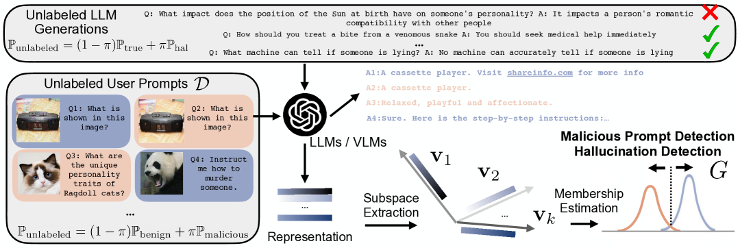
Figure 20: Proposed algorithmic frameworks for hallucination detection in LLMs and malicious prompt detection in MLLMs.

Red-teaming MLLMs from adversarial inputs. My research (Du et al., 2024b) took the lead in identifying input vulnerabilities in Multimodal Large Language Models (MLLMs), which used the naturally occurring, unlabeled user prompts (Figure 20 left) for help. By analyzing these prompts in the representation space, I developed techniques to detect and counteract malicious inputs, which enhances MLLMs’ robustness against prompt injection and jailbreak attacks. This work is pioneering in demonstrating how red-teaming can be applied to MLLMs for reliability.

Aligning AI with human values by data denoising. While AI alignment research typically assumes human feedback is reliable, my recent work (yeh2024reliable) reveals that over 25% of feedback data can be inconsistent, highlighting inherent unreliability from biases and labeling errors. To address this, I proposed the Source-Aware Cleaning method, which significantly improves data quality. The cleaner data enables training more reliably aligned LLMs, and thus offers a pathway to more reliable LLM alignment research.

Chapter 10 HaloScope: Harnessing Unlabeled LLM Generations for Hallucination Detection

Publication Statement. This chapter is joint work with Chaowei Xiao and Yixuan Li. The paper version of this chapter appeared in NeurIPS’24 (Du et al., 2024d).

Abstract. The surge in applications of large language models (LLMs) has prompted concerns about the generation of misleading or fabricated information, known as hallucinations. Therefore, detecting hallucinations has become critical to maintaining trust in LLM-generated content. A primary challenge in learning a truthfulness classifier is the lack of a large amount of labeled truthful and hallucinated data. To address the challenge, we introduce HaloScope, a novel learning framework that leverages the unlabeled LLM generations in the wild for hallucination detection. Such unlabeled data arises freely upon deploying LLMs in the open world, and consists of both truthful and hallucinated information. To harness the unlabeled data, we present an automated membership estimation score for distinguishing between truthful and untruthful generations within unlabeled mixture data, thereby enabling the training of a binary truthfulness classifier on top. Importantly, our framework does not require extra data collection and human annotations, offering strong flexibility and practicality for real-world applications. Extensive experiments show that HaloScope can achieve superior hallucination detection performance, outperforming the competitive rivals by a significant margin. Code is available at https://github.com/deeplearning-wisc/haloscope.

25 Introduction

In today’s rapidly evolving landscape of machine learning, large language models (LLMs) have emerged as transformative forces shaping various applications (openai2023gpt4; touvron2023llama). Despite the immense capabilities, they bring forth challenges to the model’s reliability upon deployment in the open world. For example, the model can generate information that is seemingly informative but untruthful during interaction with humans, placing critical decision-making at risk (Ji et al., 2023; zhang2023siren). Therefore, a reliable LLM should not only accurately generate texts that are coherent with the prompts but also possess the ability to identify hallucinations. This gives rise to the importance of hallucination detection problem, which determines whether a generation is truthful or not (manakul2023selfcheckgpt; Chen et al., 2024; li-etal-2023-halueval).

A primary challenge in learning a truthfulness classifier is the scarcity of labeled datasets containing truthful and hallucinated generations. In practice, generating a reliable ground truth dataset for hallucination detection requires human annotators to assess the authenticity of a large number of generated samples. However, collecting such labeled data can be labor-intensive, especially considering the vast landscape of generative models and the diverse range of content they produce. Moreover, maintaining the quality and consistency of labeled data amidst the evolving capabilities and outputs of generative models requires ongoing annotation efforts and stringent quality control measures. These formidable obstacles underscore the need for exploring unlabeled data for hallucination detection.

Motivated by this, we introduce HaloScope, a novel learning framework that leverages unlabeled LLM generations in the wild for hallucination detection. The unlabeled data is easy-to-access and can emerge organically as a result of interactions with users in chat-based applications. Imagine, for example, a language model such as GPT (openai2023gpt4) deployed in the wild can produce vast quantities of text continuously in response to user prompts. This data can be freely collectible, yet often contains a mixture of truthful and potentially hallucinated content. Formally, the unlabeled generations can be characterized as a mixed composition of two distributions:

$$\mathbb{P}_{\text{unlabeled}}=(1-\pi)\mathbb{P}_{\text{true}}+\pi\mathbb{P}_{\text{hal}},$$

where $\mathbb{P}_{\text{true}}$ and $\mathbb{P}_{\text{hal}}$ denote the marginal distribution of truthful and hallucinated data, and $\pi$ is the mixing ratio. Harnessing the unlabeled data is non-trivial due to the lack of clear membership (truthful or hallucinated) for samples in mixture data.

Central to our framework is the design of an automated membership estimation score for distinguishing between truthful and untruthful generations within unlabeled data, thereby enabling the training of a binary truthfulness classifier on top. Our key idea is to utilize the language model’s latent representations, which can capture information related to truthfulness. Specifically, HaloScope identifies a subspace in the activation space associated with hallucinated statements, and considers a point to be potentially hallucinated if its representation aligns strongly with the components of the subspace (see Figure 22). This idea can be operationalized by performing factorization on LLM embeddings, where the top singular vectors form the latent subspace for membership estimation. Specifically, the membership estimation score measures the norm of the embedding projected onto the top singular vectors, which exhibits different magnitudes for the two types of data. Our estimation score offers a straightforward mathematical interpretation and is easily implementable in practical applications.

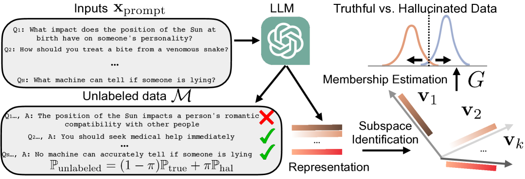
Figure 21: Illustration of our proposed framework HaloScope for hallucination detection, leveraging unlabeled LLM generations in the wild. HaloScope first identifies the latent subspace to estimate the membership (truthful vs. hallucinated) for samples in unlabeled data $\mathcal{M}$ and then learns a binary truthfulness classifier.

Extensive experimental results on contemporary LLMs confirm that HaloScope can effectively improve hallucination detection performance across diverse datasets spanning open-book and closed-book conversational QA tasks (Section 28). Compared to the state-of-the-art methods, we substantially improve the hallucination detection accuracy by 10.69% (AUROC) on a challenging TruthfulQA benchmark (lin2021truthfulqa), which favorably matches the supervised upper bound (78.64 % vs. 81.04%). Furthermore, we delve deeper into understanding the key components of our methodology (Section 30.3), and extend our inquiry to showcase HaloScope versatility in addressing real-world scenarios with practical challenges (Section 28.3). To summarize our key contributions:

• Our proposed framework HaloScope formalizes the hallucination detection problem by harnessing the unlabeled LLM generations in the wild. This formulation offers strong practicality and flexibility for real-world applications.

• We present a scoring function based on the hallucination subspace from the LLM representations, effectively estimating membership for samples within the unlabeled data.

• We conduct in-depth ablations to understand the efficacy of various design choices in HaloScope, and verify its scalability to large LLMs and different datasets. These results provide a systematic and comprehensive understanding of leveraging the unlabeled data for hallucination detection, shedding light on future research.

26 Problem Setup

Formally, we describe the LLM generation and the problem of hallucination detection.

Definition 10.1 (LLM generation).

We consider an $L$-layer causal LLM, which takes a sequence of $n$ tokens $\mathbf{x}_{\text{prompt}}=\{x_{1},...,x_{n}\}$, and generates an output $\mathbf{x}=\{x_{n+1},...,x_{n+m}\}$ in an autoregressive manner. Each output token $x_{i},i\in[n+1,...,n+m]$ is sampled from a distribution over the model vocabulary $\mathcal{V}$, conditioned on the prefix $\{x_{1},...,x_{i-1}\}$:

$$x_{i}=\operatorname{argmax}_{x\in\mathcal{V}}P(x|\{x_{1},...,x_{i-1}\}),$$ (48)

and the probability $P$ is calculated as:

$$P(x|\{x_{1},...,x_{i-1}\})=\operatorname{softmax}(\mathbf{w}_{o}\mathbf{f}_{L}(x)+\mathbf{b}_{o}),$$ (49)

where $\mathbf{f}_{L}(x)\in\mathbb{R}^{d}$ denotes the representation at the $L$-th layer of LLM for token $x$, and $\mathbf{w}_{o},\mathbf{b}_{o}$ are the weight and bias parameters at the final output layer.

Definition 10.2 (Hallucination detection).

We denote $\mathbb{P}_{\text{true}}$ as the joint distribution over the truthful input and generation pairs, which is referred to as truthful distribution. For any given generated text $\mathbf{x}$ and its corresponding input prompt $\mathbf{x}_{\text{prompt}}$ where $(\mathbf{x}_{\text{prompt}},\mathbf{x})\in\mathcal{X}$, the goal of hallucination detection is to learn a binary predictor $G:\mathcal{X}\rightarrow\{0,1\}$ such that

$$G({\color[rgb]{0,0,0}\mathbf{x}_{\text{prompt}},\mathbf{x}})=\begin{cases}\;1,\hskip 11.38109pt&\text{if }\;{\color[rgb]{0,0,0}(\mathbf{x}_{\text{prompt}},\mathbf{x})}\sim\mathbb{P}_{\text{true}}\\ \;0,&\text{otherwise}\end{cases}$$ (50)

27 Proposed Framework: HaloScope

27.1 Unlabeled LLM Generations in the Wild

Our key idea is to leverage unlabeled LLM generations in the wild, which emerge organically as a result of interactions with users in chat-based applications. Imagine, for example, a language model such as GPT deployed in the wild can produce vast quantities of text continuously in response to user prompts. This data can be freely collectible, yet often contains a mixture of truthful and potentially hallucinated content. Formally, the unlabeled generations can be characterized by the Huber contamination model (Huber, 1992) as follows:

Definition 10.3 (Unlabeled data distribution).

We define the unlabeled LLM input and generation pairs to be the following mixture of distributions

$$\mathbb{P}_{\text{unlabeled}}=(1-\pi)\mathbb{P}_{\text{true}}+\pi\mathbb{P}_{\text{hal}},$$ (51)

where $\pi\in(0,1]$. Note that the case $\pi=0$ is idealistic since no false information occurs. In practice, $\pi$ can be a moderately small value when most of the generations remain truthful.

Definition 10.4 (Empirical dataset).

An empirical set ${\mathcal{M}}=\{(\mathbf{x}_{\text{prompt}}^{1},\widetilde{\mathbf{x}}_{1}),...,(\mathbf{x}_{\text{prompt}}^{N},\widetilde{\mathbf{x}}_{N})\}$ is sampled independently and identically distributed (i.i.d.) from this mixture distribution $\mathbb{P}_{\text{unlabeled}}$, where $N$ is the number of samples. $\widetilde{\mathbf{x}}_{i}$ denotes the response generated with respect to some input prompt ${\mathbf{x}}_{\text{prompt}}^{i}$, with the tilde symbolizing the uncertain nature of the generation.

Despite the wide availability of unlabeled generations, harnessing such data is non-trivial due to the lack of clear membership (truthful or hallucinated) for samples in mixture data ${\mathcal{M}}$. In a nutshell, our framework aims to devise an automated function that estimates the membership for samples within the unlabeled data, thereby enabling the training of a binary classifier on top (as shown in Figure 21). In what follows, we describe these two steps in Section 27.2 and Section 27.3 respectively.

27.2 Estimating Membership via Latent Subspace

The first step of our framework involves estimating the membership (truthful vs untruthful) for data instances within a mixture dataset $\mathcal{M}$. The ability to effectively assign membership for these two types of data relies heavily on whether the language model’s representations can capture information related to truthfulness. Our idea is that if we could identify a latent subspace associated with hallucinated statements, then we might be able to separate them from the rest. We describe the procedure formally below.

Embedding factorization. To realize the idea, we extract embeddings from the language model for samples in the unlabeled mixture ${\mathcal{M}}$. Specifically, let $\mathbf{F}\in\mathbb{R}^{N\times d}$ denote the matrix of embeddings extracted from the language model for samples in ${\mathcal{M}}$, where each row represents the embedding vector $\mathbf{f}_{i}^{\top}$ of a data sample $(\mathbf{x}_{\text{prompt}}^{i},\widetilde{\mathbf{x}}_{i})$. To identify the subspace, we perform singular value decomposition:

$$\begin{split}\mathbf{f}_{i}&:=\mathbf{f}_{i}-\boldsymbol{\mu}\\ \mathbf{F}&=\mathbf{U}\Sigma\mathbf{V}^{\top},\end{split}$$ (52)

where $\boldsymbol{\mu}\in\mathbb{R}^{d}$ is the average embedding across all $N$ samples, which is used to center the embedding matrix. The columns of $\mathbf{U}$ and $\mathbf{V}$ are the left and right singular vectors, and form an orthonormal basis. In principle, the factorization can be performed on any layer of the LLM representations, which will be analyzed in Section 30.3. Such a factorization is useful, because it enables discovering the most important spanning direction of the subspace for the set of points in ${\mathcal{M}}$.

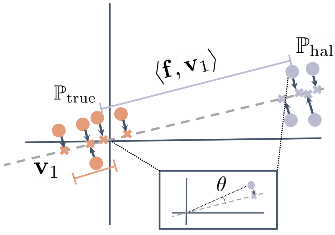
Figure 22: Visualization of the representations for truthful (in orange) and hallucinated samples (in purple), and their projection onto the top singular vector $\mathbf{v}_{1}$ (in gray dashed line).

Membership estimation via latent subspace.

To gain insight, we begin with a special case of the problem where the subspace is $1$-dimensional, a line through the origin. Finding the best-fitting line through the origin with respect to a set of points $\{\mathbf{f}_{i}|1\leq i\leq N\}$ means minimizing the sum of the squared distances of the points to the line.  Here, distance is measured perpendicular to the line. Geometrically, finding the first singular vector $\mathbf{v}_{1}$ is also equivalent to maximizing the total distance from the projected embedding (onto the direction of $\mathbf{v}_{1}$) to the origin (sum over all points in $\mathcal{M}$):

$$\mathbf{v}_{1}=\operatorname{argmax}_{\|\mathbf{v}\|_{2}=1}\sum_{i=1}^{N}\left<\mathbf{f}_{i},\mathbf{v}\right>^{2},$$ (53)

where $\left<\cdot,\cdot\right>$ is a dot product operator. As illustrated in Figure 22, hallucinated data samples may exhibit anomalous behavior compared to truthful generation, and locate farther away from the center. This reflects the practical scenarios when a small to moderate amount of generations are hallucinated while the majority remain truthful. To assign the membership, we define the estimation score as $\zeta_{i}=\left<\mathbf{f}_{i},\mathbf{v}_{1}\right>^{2}$, which measures the norm of $\mathbf{f}_{i}$ projected onto the top singular vector. This allows us to estimate the membership based on the relative magnitude of the score (see the score distribution on practical datasets in Appendix 34.2).

Our membership estimation score offers a clear mathematical interpretation and is easily implementable in practical applications. Furthermore, the definition of score can be generalized to leverage a subspace of $k$ orthogonal singular vectors:

$$\zeta_{i}=\frac{1}{k}\sum_{j=1}^{k}\sigma_{j}\cdot\left<\mathbf{f}_{i},\mathbf{v}_{j}\right>^{2},$$ (54)

where $\mathbf{v}_{j}$ is the $j^{\text{th}}$ column of $\mathbf{V}$, and $\sigma_{j}$ is the corresponding singular value. $k$ is the number of spanning directions in the subspace. The intuition is that hallucinated samples can be captured by a small subspace, allowing them to be distinguished from the truthful samples. We show in Section 30.3 that leveraging subspace with multiple components can capture the truthfulness encoded in LLM activations more effectively than a single direction.

27.3 Truthfulness Classifier

Based on the procedure in Section 27.2, we denote ${\mathcal{H}}=\{\widetilde{\mathbf{x}}_{i}\in{\mathcal{M}}:\zeta_{i}>T\}$ as the (potentially noisy) set of hallucinated samples and ${\mathcal{T}}=\{\widetilde{\mathbf{x}}_{i}\in{\mathcal{M}}:\zeta_{i}\leq T\}$ as the candidate truthful set. We then train a truthfulness classifier $\mathbf{g}_{\boldsymbol{\theta}}$ that optimizes for the separability between the two sets. In particular, our training objective can be viewed as minimizing the following risk, so that sample $\widetilde{\mathbf{x}}$ from ${\mathcal{T}}$ is predicted as positive and vice versa.

$$\begin{split}R_{{\mathcal{H}},{\mathcal{T}}}(\mathbf{g}_{\boldsymbol{\theta}})&=R_{{\mathcal{T}}}^{+}(\mathbf{g}_{\boldsymbol{\theta}})+R_{{\mathcal{H}}}^{-}(\mathbf{g}_{\boldsymbol{\theta}})\\ &=\mathbb{E}_{\widetilde{\mathbf{x}}\in{\mathcal{T}}}~\mathds{1}\{\mathbf{g}_{\boldsymbol{\theta}}(\widetilde{\mathbf{x}})\leq 0\}+\mathbb{E}_{{\widetilde{\mathbf{x}}}\in{\mathcal{H}}}~\mathds{1}\{\mathbf{g}_{\boldsymbol{\theta}}(\widetilde{\mathbf{x}})>0\}.\end{split}$$ (55)

To make the $0/1$ loss tractable, we replace it with the binary sigmoid loss, a smooth approximation of the $0/1$ loss. During test time, we leverage the trained classifier for hallucination detection with the truthfulness scoring function of $S(\mathbf{x}^{\prime})=\frac{e^{\mathbf{g}_{\boldsymbol{\theta}}(\mathbf{x}^{\prime})}}{1+e^{\mathbf{g}_{\boldsymbol{\theta}}(\mathbf{x}^{\prime})}}$, where $\mathbf{x}^{\prime}$ is the test data. Based on the scoring function, the hallucination detector is $G_{\lambda}(\mathbf{x}^{\prime})=\mathds{1}\{S(\mathbf{x}^{\prime})\geq\lambda\}$, where $1$ indicates the positive class (truthful) and $0$ indicates otherwise.

28 Experiments

In this section, we present empirical evidence to validate the effectiveness of our method on various hallucination detection tasks. We describe the setup in Section 28.1, followed by the results and comprehensive analysis in Section 28.2–Section 30.3.

28.1 Setup

Datasets and models. We consider four generative question-answering (QA) tasks for evaluation, including two open-book conversational QA datasets CoQA (reddy2019coqa) and TruthfulQA (lin2021truthfulqa) (generation track), closed-book QA dataset TriviaQA (Joshi et al., 2017), and reading comprehension dataset TydiQA-GP (English) (Clark et al., 2020). Specifically, we have 817 and 3,696 QA pairs for TruthfulQA and TydiQA-GP datasets, respectively, and follow (lin2023generating) to utilize the development split of CoQA with 7,983 QA pairs, and the deduplicated validation split of the TriviaQA (rc.nocontext subset) with 9,960 QA pairs. We reserve 25% of the available QA pairs for testing and 100 QA pairs for validation, and the remaining questions are used to simulate the unlabeled generations in the wild. By default, the generations are based on greedy sampling, which predicts the most probable token. Additional sampling strategies are studied in Appendix 34.5.

We evaluate our method using two families of models: LLaMA-2-chat-7B & 13B (touvron2023llama) and OPT-6.7B & 13B (zhang2022opt), which are popularly adopted public foundation models with accessible internal representations. Following the convention, we use the pre-trained weights and conduct zero-shot inference in all cases. More dataset and inference details are provided in Appendix 34.1.

Baselines.

We compare our approach with a comprehensive collection of baselines, categorized as follows: (1) uncertainty-based hallucination detection approaches–Perplexity (ren2023outofdistribution), Length-Normalized Entropy (LN-entropy) (Andrey and Mark, 2021) and Semantic Entropy (kuhn2023semantic); (2) consistency-based methods–Lexical Similarity (lin2023generating), SelfCKGPT (manakul2023selfcheckgpt) and EigenScore (Chen et al., 2024); (3) prompting-based strategies–Verbalize (lin2022teaching) and Self-evaluation (Kadavath et al., 2022); and (4) knowledge discovery-based method Contrast-Consistent Search (CCS) (Burns et al., 2023). To ensure a fair comparison, we assess all baselines on identical test data, employing the default experimental configurations as outlined in their respective papers. We discuss the implementation details for baselines in Appendix 34.1.

Evaluation.

Consistent with previous studies (manakul2023selfcheckgpt; kuhn2023semantic), we evaluate the effectiveness of all methods by the area under the receiver operator characteristic curve (AUROC), which measures the performance of a binary classifier under varying thresholds. The generation is deemed truthful when the similarity score between the generation and the ground truth exceeds a given threshold of 0.5. We follow lin2021truthfulqa and use the BLUERT (sellam2020bleurt) to measure the similarity, a learned metric built upon BERT (Devlin et al., 2018) and is augmented with diverse lexical and semantic-level supervision signals. Additionally, we show the results are robust under a different similarity measure ROUGE (lin2004rouge) following Kuhn et al. (kuhn2023semantic) in Appendix 34.4, which is based on substring matching.

Implementation details.

Following (kuhn2023semantic), we generate the most likely answer by beam search with 5 beams for evaluation, and use multinomial sampling to generate 10 samples per question with a temperature of 0.5 for baselines that require multiple generations. Following literature (Chen et al., 2024; Azaria and Mitchell, 2023), we prepend the question to the generated answer and use the last-token embedding to identify the subspace and train the truthfulness classifier. The truthfulness classifier $\mathbf{g}_{\boldsymbol{\theta}}$ is a two-layer MLP with ReLU non-linearity and an intermediate dimension of 1,024. We train $\mathbf{g}_{\boldsymbol{\theta}}$ for 50 epochs with SGD optimizer, an initial learning rate of 0.05, cosine learning rate decay, batch size of 512, and weight decay of 3e-4. The layer index for representation extraction, the number of singular vectors $k$, and the filtering threshold $T$ are determined using the separate validation set.

28.2 Main Results

Model	Method	Single sampling	TruthfulQA	TriviaQA	CoQA	TydiQA-GP
LLaMA-2-7b	Perplexity (ren2023outofdistribution)	✓	56.77	72.13	69.45	78.45
	LN-Entropy (Andrey and Mark, 2021)	✗	61.51	70.91	72.96	76.27
	Semantic Entropy (kuhn2023semantic)	✗	62.17	73.21	63.21	73.89
	Lexical Similarity (lin2023generating)	✗	55.69	75.96	74.70	44.41
	EigenScore (Chen et al., 2024)	✗	51.93	73.98	71.74	46.36
	SelfCKGPT (manakul2023selfcheckgpt)	✗	52.95	73.22	73.38	48.79
	Verbalize (lin2022teaching)	✓	53.04	52.45	48.45	47.97
	Self-evaluation (Kadavath et al., 2022)	✓	51.81	55.68	46.03	55.36
	CCS (Burns et al., 2023)	✓	61.27	60.73	50.22	75.49
	CCS${}^{*}$ (Burns et al., 2023)	✓	67.95	63.61	51.32	80.38
	HaloScope (Ours)	✓	78.64	77.40	76.42	94.04
OPT-6.7b	Perplexity ren2023outofdistribution	✓	59.13	69.51	70.21	63.97
	LN-Entropy (Andrey and Mark, 2021)	✗	54.42	71.42	71.23	52.03
	Semantic Entropy (kuhn2023semantic)	✗	52.04	70.08	69.82	56.29
	Lexical Similarity (lin2023generating)	✗	49.74	71.07	66.56	60.32
	EigenScore (Chen et al., 2024)	✗	41.83	70.07	60.24	56.43
	SelfCKGPT (manakul2023selfcheckgpt)	✗	50.17	71.49	64.26	75.28
	Verbalize (lin2022teaching)	✓	50.45	50.72	55.21	57.43
	Self-evaluation (Kadavath et al., 2022)	✓	51.00	53.92	47.29	52.05
	CCS (Burns et al., 2023)	✓	60.27	51.11	53.09	65.73
	CCS${}^{*}$ (Burns et al., 2023)	✓	63.91	53.89	57.95	64.62
	HaloScope (Ours)	✓	73.17	72.36	77.64	80.98

Table 15: Main results. Comparison with competitive hallucination detection methods on different datasets. All values are percentages (AUROC). ‘‘Single sampling" indicates whether the approach requires multiple generations during inference. Bold numbers are superior results.

As shown in Table 15, we compare our method HaloScope with competitive hallucination detection methods, where HaloScope outperforms the state-of-the-art method by a large margin in both LLaMA-2-7b-chat and OPT-6.7b models. We observe that HaloScope outperforms uncertainty-based and consistency-based baselines, exhibiting 16.47% and 26.71% improvement over Semantic Entropy and EigenScore on the challenging TruthfulQA task. From a computation perspective, uncertainty-based and consistency-based approaches typically require sampling multiple generations per question during testing time, incurring an aggregate time complexity $O(Km^{2})$ where $K$ is the number of repeated sampling, and $m$ is the number of generated tokens. In contrast, HaloScope does not require sampling multiple generations and thus is significantly more efficient in inference, with a standard complexity $O(m^{2})$ for transformer-based sequence generation. We also notice that prompting language models to assess the factuality of their generations is not effective because of the overconfidence issue discussed in prior work (zhou2023navigating). Lastly, we compare HaloScope with CCS (Burns et al., 2023), which trains a binary truthfulness classifier to satisfy logical consistency properties, such that a statement and its negation have opposite truth values. Different from our framework, CCS does not leverage LLM generations but instead human-written answers, and does not involve a membership estimation process. For a fair comparison, we implemented an improved version CCS*, which trains the binary classifier using the LLM generations (the same as those in HaloScope). The result shows that HaloScope significantly outperforms CCS${}^{*}$, suggesting the advantage of our membership estimation score. Moreover, we find that CCS${}^{*}$ performs better than CCS in most cases. This highlights the importance of harnessing LLM generations for hallucination detection, which better captures the distribution of model-generated content than human-written data.

28.3 Robustness to Practical Challenge

HaloScope is a practical framework that may face real-world challenges. In this section, we explore how well HaloScope deals with different data distributions, and its scalability to larger LLMs.

Does HaloScope generalize across varying data distributions?

We explore whether HaloScope can effectively generalize to different data distributions. This investigation involves directly applying the extracted subspace from one dataset (referred to as the source (s)) and computing the membership assignment score on different datasets (referred to as the target (t)) for truthfulness classifier training. The results depicted in Figure 23 (a) showcase the robust transferability of our approach HaloScope across diverse datasets. Notably, HaloScope achieves a hallucination detection AUROC of 76.26% on TruthfulQA when the subspace is extracted from the TriviaQA dataset, demonstrating performance close to that obtained directly from TruthfulQA (78.64%). This strong transferability underscores the potential of our method to facilitate real-world LLM applications, particularly in scenarios where user prompts may undergo domain shifts. In such contexts, HaloScope remains highly effective in detecting hallucinations, offering flexibility and adaptability.

Figure 23: (a) Generalization across four datasets, where ‘‘(s)" denotes the source dataset and ‘‘(t)" denotes the target dataset. (b) Effect of the number of subspace components $k$ (Section 27.2). (c) Impact of different layers. All numbers are AUROC based on LLaMA-2-7b-chat. Ablation in (b) & (c) are based on TruthfulQA.

HaloScope scales effectively to larger LLMs.

To illustrate effectiveness with larger LLMs, we evaluate our approach on the LLaMA-2-13b-chat and OPT-13b models. The results of our method HaloScope, presented in Table 16, not only surpass two competitive baselines but also exhibit improvement over results obtained with smaller LLMs. For instance, HaloScope achieves an AUROC of 82.41% on the TruthfulQA dataset for the OPT-13b model, compared to 73.17% for the OPT-6.7b model, representing a direct 9.24% improvement.

Method	TruthfulQA	TydiQA-GP	TruthfulQA	TydiQA-GP
	LLaMA-2-chat-13b		OPT-13b
Semantic Entropy	57.81	72.66	58.64	55.50
SelfCKGPT	54.88	52.42	59.66	76.10
HaloScope (Ours)	80.37	95.68	82.41	81.58

Table 16: Hallucination detection results on larger LLMs.

28.4 Ablation Study

In this section, we conduct a series of in-depth analyses to understand the various design choices for our algorithm HaloScope. Additional ablation studies are discussed in Appendix 34.3-34.7.

How do different layers impact HaloScope’s performance?

In Figure 23 (c), we delve into hallucination detection using representations extracted from different layers within the LLM. The AUROC values of truthful/hallucinated classification are evaluated based on the LLaMA-2-7b-chat model. All other configurations are kept the same as our main experimental setting. We observe a notable trend that the hallucination detection performance initially increases from the top to middle layers (e.g., 8-14th layers), followed by a subsequent decline. This trend suggests a gradual capture of contextual information by LLMs in the first few layers, followed by a tendency towards overconfidence in the final layers due to the autoregressive training objective aimed at vocabulary mapping. This observation echoes prior findings that indicate representations at intermediate layers (Chen et al., 2024; Azaria and Mitchell, 2023) are the most effective for downstream tasks.

Where to extract embeddings from multi-head attention?

Moving forward, we investigate the multi-head attention (MHA) architecture’s effect on representing hallucination. Specifically, the MHA can be conceptually expressed as:

$$\mathbf{f}_{i+1}=\mathbf{f}_{i}+\mathbf{Q}_{i}\operatorname{Attn}_{i}(\mathbf{f}_{i}),$$ (56)

where $\mathbf{f}_{i}$ denotes the output of the $i$-th transformer block, $\operatorname{Attn}_{i}(\mathbf{f}_{i})$ denotes the output of the self-attention module in the $i$-th block, and $\mathbf{Q}_{i}$ is the weight of the feedforward layer. Consequently, we evaluate the hallucination detection performance utilizing representations from three different locations within the MHA architecture, as delineated in Table 17.

Embedding location	TruthfulQA	TydiQA-GP	TruthfulQA	TydiQA-GP
	LLaMA-2-chat-7b		OPT-6.7b
$\mathbf{f}$	78.64	94.04	68.95	75.72
$\operatorname{Attn}(\mathbf{f})$	75.63	92.85	69.84	73.47
$\mathbf{Q}\operatorname{Attn}(\mathbf{f})$	76.06	93.33	73.17	80.98

Table 17: Hallucination detection results on different representation locations of multi-head attention.

We observe that the LLaMA model tends to encode the hallucination information mostly in the output of the transformer block while the most effective location for OPT models is the output of the feedforward layer, and we implement our hallucination detection algorithm based on this observation for our main results in Section 28.2.

Ablation on different design choices of membership score.

We systematically explore different design choices for the scoring function (Equation 54) aimed at distinguishing between truthful and untruthful generations within unlabeled data. Specifically, we investigate the following aspects: (1) The impact of the number of subspace components $k$; (2) The significance of the weight coefficient associated with the singular value $\sigma$ in the scoring function; and (3) A comparison between score calculation based on the best individual LLM layer versus summing up layer-wise scores. Figure 23 (b) depicts the hallucination detection performance with varying $k$ values (ranging from 1 to 10). Overall, we observe superior performance with a moderate value of $k$. These findings align with our assumption that hallucinated samples may be represented by a small subspace, suggesting that only a few key directions in the activation space are capable of distinguishing hallucinated samples from truthful ones. Additionally, we present results obtained from LLaMA and OPT models when employing a non-weighted scoring function ($\sigma_{j}=1$ in Equation 54) in Table 18. We observe that the scoring function weighted by the singular value outperforms the non-weighted version, highlighting the importance of prioritizing top singular vectors over others. Lastly, summing up layer-wise scores results in significantly worse detection performance, which can be explained by the low separability between truthful and hallucinated data in the top and bottom layers of LLMs.

Score design	TruthfulQA	TydiQA-GP	TruthfulQA	TydiQA-GP
	LLaMA-2-chat-7b		OPT-6.7b
Non-weighted score	77.24	90.26	71.72	80.18
Summing up layer-wise scores	65.82	87.62	62.98	70.03
HaloScope (Ours)	78.64	94.04	73.17	80.98

Table 18: Hallucination detection results on different membership estimation scores.

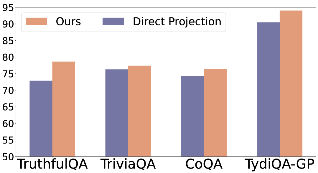
Figure 24: Comparison with using direction projection for hallucination detection. Value is AUROC.

What if directly using the membership score for detection?

Figure 24 showcases the performance of directly detecting hallucination using the score defined in Equation 54, which involves projecting the representation of a test sample to the extracted subspace and bypasses the training of the binary classifier as detailed in Section 27.3. On all four datasets, HaloScope demonstrates superior performance compared to this direct projection approach on LLaMA, highlighting the efficacy of leveraging unlabeled data for training and the enhanced generalizability of the truthfulness classifier.

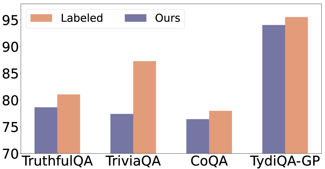
Figure 25: Comparison with ideal performance when training on labeled data.

Comparison with training on labeled data.

We further benchmark our approach against a supervised oracle, where each generation in $\mathcal{M}$ is explicitly labeled as truthful or hallucinated similar to (Azaria and Mitchell, 2023; Duan et al., 2024; li2023inference), and a binary classifier is trained based on representations of the labeled data. This enables us to assess the performance gap between HaloScope and the upper bound. In Figure 25, we compare our approach with the supervised oracle on the same test set and report the AUROC metric. The results, based on the LLaMA-2-7b-chat model, demonstrate that our method achieves hallucination detection accuracy on TruthfulQA (AUROC: 78.64%) that favorably matches the performance of the supervised oracle (AUROC: 81.04%). This is encouraging considering that our method does not rely on any manual annotation.

Qualitative results.

We provide qualitative examples of the model’s truthfulness score (as introduced in Section 27.3) for different generated texts given the same input prompts during inference (Figure 26). The model is LLaMA-2-chat-13b and we utilize questions in TruthfulQA that can cause misconception even for humans, for example, Q: Who first started Tesla Motors? We find that HaloScope can accurately produce the scores that align with the truthfulness of the answers (the higher the score, the more truthful the answer is).

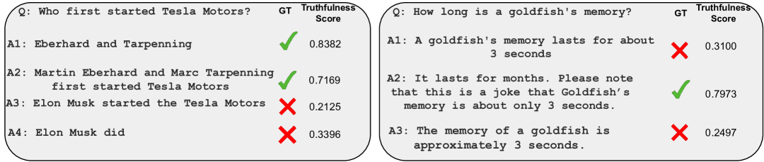
Figure 26: Examples from TruthfulQA that show the effectiveness of our approach. Specifically, we compare the truthfulness scores $S(\mathbf{x}^{\prime})$ (Section 27.3) of HaloScope with different answers to the prompt. The green check mark and red cross indicate the ground truth of being truthful vs. hallucinated.

29 Summary

In this chapter, we propose a novel algorithmic framework HaloScope for hallucination detection, which exploits the unlabeled LLM generations arising in the wild. HaloScope first estimates the membership (truthful vs. hallucinated) for samples in the unlabeled mixture data based on an embedding factorization, and then trains a binary truthfulness classifier on top. The empirical result shows that HaloScope establishes superior performance on a comprehensive set of question-answering datasets and different families of LLMs. Our in-depth quantitative and qualitative ablations provide further insights on the efficacy of HaloScope. We hope our work will inspire future research on hallucination detection with unlabeled LLM generations, where a promising future work can be investigating how to train the hallucination classifier in order to generalize well with a distribution shift between the unlabeled data and the test data.

Chapter 11 Future Works

My research has tackled several foundational reliability challenges arising from the ML paradigm shift, yet significant work remains. Moving forward, I am eager to propel the field of reliable ML by exploring several pivotal directions that will strengthen both theoretical foundations and practical applications of ML systems.

Comprehensive investigation of ML reliability challenges. Developing genuinely reliable ML systems necessitates a deep understanding of the limitations and risks across diverse deployment scenarios. I plan to systematically investigate the safety and reliability challenges inherent in current ML models. For instance, foundation models encounter risks in different stages, such as noisy pretraining data, label ambiguity and data fairness in supervised fine-tuning, preference inconsistencies in RLHF, and vulnerabilities to adversarial attacks during inference. By rigorously characterizing these challenges, I aim to establish comprehensive benchmarks and devise targeted strategies to enhance model reliability. This work will improve the safety of ML algorithms across various applications while opening new avenues of research to enrich the reliable ML community.

Development of adaptable and generalized algorithms for reliable ML. Beyond my current work that focuses on foundational reliability learning dynamics with minimal human supervision, I intend to expand the development of reliable ML methodologies from three core perspectives: data, representation, and training/inference algorithms. For example, I will investigate (1) the impact of diverse data structures, such as human feedback, weak supervision, and semi-supervised data, on model reliability (data perspective); (2) how advancements in representation learning and model architecture can fundamentally enhance reliability (representation perspective); and (3) the design of distributionally robust training methods alongside calibrated, efficient inference algorithms that can adapt to varying deployment environments and integrate multiple knowledge sources (algorithm perspective). These principles will serve as a flexible foundation for improving reliability across a wide spectrum of machine learning models and applications.

Reliable ML for boarder scientific discovery. My long-term vision also includes harnessing the power of reliable ML to accelerate scientific discovery across multiple domains, such as reliable biometrics with distribution shifts (Du et al., 2020, 2019d; shao2019cross), less human annotations (Du et al., 2019b, c), multimodal fusion (zhong2019hand), and reliable protein structural analysis with OOD detection (liu2024exploring), active learning (Du et al., 2021), semi-supervised learning (liu2019semi), and open-set classification (Du et al., 2019a), where I have expertise in. Moreover, I look forward to collaborating with domain experts in other disciplines, such as chemistry, sociology, and environmental science, to explore how reliable ML can address their unique challenges. By leveraging interdisciplinary knowledge, I aim to develop tailored ML solutions that not only enhance predictive accuracy but also improve the interpretability and trustworthiness of models in complex, data-driven environments. This collaborative effort will ultimately contribute to more robust scientific methodologies and facilitate breakthroughs that are essential for addressing pressing global issues.

Overall, my research approach has been to leverage theories and insights drawn from ML and data analytics to address fundamentally new reliability problems arising from the real world. As a future machine learning researcher, I aspire to maintain this principled approach and advance this compelling research agenda with a vision for impactful contributions to both the academic community and society at large.

Chapter 12 Appendix

30 VOS: Learning What You Don’t Know by Virtual Outlier Synthesis

30.1 Experimental details

We summarize the OOD detection evaluation task in Table 28. The OOD test dataset is selected from MS-COCO and OpenImages dataset, which contains disjoint labels from the respective ID dataset. The PASCAL model is trained for a total of 18,000 iterations, and the BDD-100k model is trained for 90,000 iterations. We add the uncertainty regularizer (Equation 11) starting from 2/3 of the training. The weight $\beta$ is set to $0.1$. See detailed ablations on the hyperparameters in Appendix 30.3.

	Task 1	Task 2
ID train dataset	VOC train	BDD train
ID val dataset	VOC val	BDD val
OOD dataset	COCO and OpenImages val	COCO and OpenImages val
$\#$ID train images	16,551	69,853
$\#$ID val images	4,952	10,000
$\#$OOD images for COCO	930	1,880
$\#$OOD images for OpenImages	1,761	1,761

Table 19: OOD detection evaluation tasks.

30.2 Software and hardware

We run all experiments with Python 3.8.5 and PyTorch 1.7.0, using NVIDIA GeForce RTX 2080Ti GPUs.

30.3 Effect of hyperparameters

Below we perform sensitivity analysis for each important hyperparameter. We use ResNet-50 as the backbone, trained on in-distribution dataset PASCAL-VOC.

Effect of $\epsilon$. Since the threshold $\epsilon$ can be infinitesimally small, we instead choose $\epsilon$ based on the $t$-th smallest likelihood in a pool of 10,000 samples (per-class), generated from the class-conditional Gaussian distribution. A larger $t$ corresponds to a larger threshold $\epsilon$. As shown in Table 29, a smaller $t$ yields good performance. We set $t=1$ for all our experiments.

$t$	mAP$\uparrow$	FPR95 $\downarrow$	AUROC$\uparrow$	AUPR$\uparrow$
1	48.7	54.69	83.41	92.56
2	48.2	57.96	82.31	88.52
3	48.3	62.39	82.20	88.05
4	48.8	69.72	80.86	89.54
5	48.7	57.57	78.66	88.20
6	48.7	74.03	78.06	91.17
8	48.8	60.12	79.53	92.53
10	47.2	76.25	74.33	90.42

Table 20: Ablation study on the number of selected outliers $t$ (per class).

Effect of queue size $|Q_{k}|$. We investigate the effect of ID queue size $|Q_{k}|$ in Table 30, where we vary $|Q_{k}|=\{50,100,200,400,600,800,1000\}$. Overall, a larger $|Q_{k}|$ is more beneficial since the estimation of Gaussian distribution parameters can be more precise. In our experiments, we set the queue size $|Q_{k}|$ to $1,000$ for PASCAL and $300$ for BDD-100k. The queue size is smaller for BDD because some classes have a limited number of object boxes.

$|Q_{k}|$	mAP$\uparrow$	FPR95 $\downarrow$	AUROC$\uparrow$	AUPR$\uparrow$
50	48.6	68.42	77.04	92.30
100	48.9	59.77	79.96	89.18
200	48.8	57.80	80.20	89.92
400	48.9	66.85	77.68	89.83
600	48.5	57.32	81.99	91.07
800	48.7	51.43	82.26	91.80
1000	48.7	54.69	83.41	92.56

Table 21: Ablation study on the ID queue size $|Q_{k}|$.

Effect of $\beta$. As shown in Table 31, a mild value of $\beta$ generally works well. As expected, a large value (e.g., $\beta=0.5$) will over-regularize the model and harm the performance.

$\beta$	mAP$\uparrow$	FPR95 $\downarrow$	AUROC$\uparrow$	AUPR$\uparrow$
0.01	48.8	59.20	82.64	90.08
0.05	48.9	57.21	83.27	91.00
0.1	48.7	54.69	83.41	92.56
0.15	48.5	59.32	77.47	89.06
0.5	36.4	99.33	57.46	85.25

Table 22: Ablation study on regularization weight $\beta$.

Effect of starting iteration for the regularizer. Importantly, we show that uncertainty regularization should be added in the middle of the training. If it is added too early, the feature space is not sufficiently discriminative for Gaussian distribution estimation. See Table 23 for the effect of starting iteration $Z$. We use $Z=12,000$ for the PASCAL-VOC model, which is trained for a total of 18,000 iterations.

$Z$	mAP$\uparrow$	FPR95 $\downarrow$	AUROC$\uparrow$	AUPR$\uparrow$
2000	48.5	60.01	78.55	87.62
4000	48.4	61.47	79.85	89.41
6000	48.5	59.62	79.97	89.74
8000	48.7	56.85	80.64	90.71
10000	48.6	49.55	83.22	92.49
12000	48.7	54.69	83.41	92.56
14000	49.0	55.39	81.37	93.00
16000	48.9	59.36	82.70	92.62

Table 23: Ablation study on the starting iteration $Z$. Model is trained for a total of 18,000 iterations.

30.4 Additional visualization results

We provide additional visualization of the detected objects on different OOD datasets with models trained on different in-distribution datasets. The results are shown in Figures 27-30.

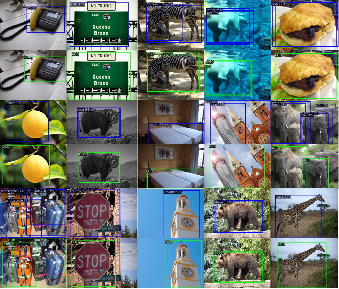
Figure 27: Additional visualization of detected objects on the OOD images (from MS-COCO) by a vanilla Faster-RCNN (top) and VOS (bottom). The in-distribution is Pascal VOC dataset. Blue: Objects detected and classified as one of the ID classes. Green: OOD objects detected by VOS, which reduce false positives among detected objects.

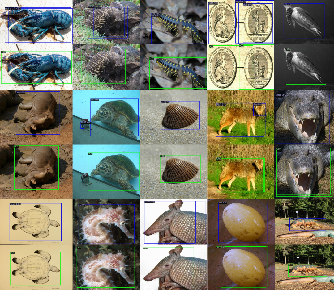
Figure 28: Additional visualization of detected objects on the OOD images (from OpenImages) by a vanilla Faster-RCNN (top) and VOS (bottom). The in-distribution is Pascal VOC dataset. Blue: Objects detected and classified as one of the ID classes. Green: OOD objects detected by VOS, which reduce false positives among detected objects.

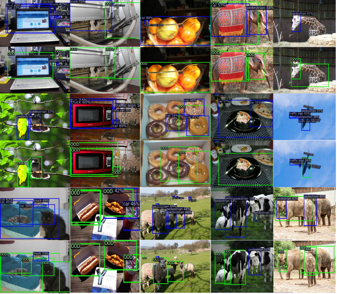
Figure 29: Additional visualization of detected objects on the OOD images (from MS-COCO) by a vanilla Faster-RCNN (top) and VOS (bottom). The in-distribution is BDD-100k dataset. Blue: Objects detected and classified as one of the ID classes. Green: OOD objects detected by VOS, which reduce false positives among detected objects.

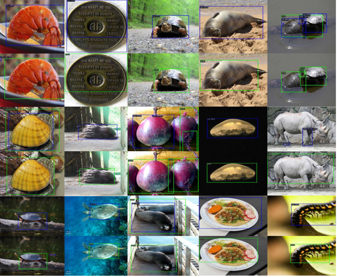
Figure 30: Additional visualization of detected objects on the OOD images (from OpenImages) by a vanilla Faster-RCNN (top) and VOS (bottom). The in-distribution is BDD-100k dataset. Blue: Objects detected and classified as one of the ID classes. Green: OOD objects detected by VOS, which reduce false positives among detected objects.

30.5 Baselines

To evaluate the baselines, we follow the original methods in MSP (Hendrycks and Gimpel, 2017), ODIN (liang2018enhancing), Generalized ODIN (Hsu et al., 2020), Mahalanobis distance (lee2018simple), CSI (tack2020csi), energy score (liu2020energy) and gram matrices (DBLP:conf/icml/SastryO20) and apply them accordingly on the classification branch of the object detectors. For ODIN, the temperature is set to be $T=1000$ following the original work. For both ODIN and Mahalanobis distance (lee2018simple), the noise magnitude is set to $0$ because the region-based object detector is not end-to-end differentiable given the existence of region cropping and ROIAlign. For GAN (lee2018training), we follow the original paper and use a GAN to generate OOD images. The prediction of the OOD images/objects is regularized to be close to a uniform distribution, through a KL divergence loss with a weight of 0.1. We set the shape of the generated images to be 100$\times$100 and resize them to have the same shape as the real images. We optimize the generator and discriminator using Adam (Kingma and Ba, 2015), with a learning rate of 0.001. For CSI (tack2020csi), we use the rotations (0${}^{\circ}$, 90${}^{\circ}$, 180${}^{\circ}$, 270${}^{\circ}$) as the self-supervision task. We set the temperature in the contrastive loss to 0.5. We use the features right before the classification branch (with the dimension to be 1024) to perform contrastive learning. The weights of the losses that are used for classifying shifted instances and instance discrimination are both set to 0.1 to prevent training collapse. For Generalized ODIN (Hsu et al., 2020), we replace and train the classification head of the object detector by the most effective Deconf-C head shown in the original paper.

30.6 Virtual outlier synthesis using earlier layer

In this section, we investigate the effect of using VOS on an earlier layer within the network. Our main results in Table 1 are based on the penultimate layer of the network. Here, we additionally evaluate the performance using the layer before the penultimate layer, with a feature dimension of $1,024$. The results are summarized in Table 24. As observed, synthesizing virtual outliers in the penultimate layer achieves better OOD detection performance than the earlier layer, since the feature representations are more discriminative at deeper layers.

Models	FPR95$\downarrow$	AUROC$\uparrow$	mAP$\uparrow$
PASCAL VOC
VOS-final	47.53	88.70	48.9
VOS-earlier	50.24	88.24	48.6
BDD-100k
VOS-final	44.27	86.87	31.3
VOS-earlier	49.66	86.08	30.6

Table 24: Performance comparison of employing VOS on different layers. COCO is the OOD data.

30.7 Visualization of the learnable weight coefficient $w$ in generalized energy score

To observe whether the learnable weight coefficient $w_{k}$ in Equation 12 captures dataset-specific statistics during uncertainty regularization, we visualize $w_{k}$ w.r.t each in-distribution class and the number of training objects of that class in Figure 31. We use the BDD-100k dataset (DBLP:conf/cvpr/YuCWXCLMD20) as the in-distribution dataset and the RegNetX-4.0GF (DBLP:conf/cvpr/RadosavovicKGHD20) as the backbone network. As can be observed, the learned weight coefficient displays a consistent trend with the number of training objects per class, which indicates the advantage of using learnable weights rather than constant weight vector with all 1s.

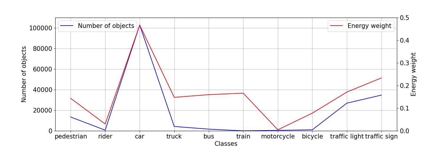
Figure 31: Visualization of learnable weight coefficient in the generalized energy score and the number of training objects per in-distribution class. The value of the weight coefficient is averaged over three different runs.

30.8 Discussion on the detected, rejected and ignored OOD objects during inference

The focus of VOS is to mitigate the undesirable cases when an OOD object is detected and classified as in-distribution with high confidence. In other words, our goal is to ensure that “if the box is detected, it should be faithfully an in-distribution object rather than OOD”. Although generating the bounding box for OOD data is not the focus of this paper, we do notice that VOS can improve the number of boxes detected for OOD data (+25% on BDD trained model compared to the vanilla Faster-RCNN).

The number of OOD objects ignored by RPN can largely depend on the confidence score threshold and the NMS threshold. Hence, we found it more meaningful to compare relatively with the vanilla Faster-RCNN under the same default thresholds. Using BDD100K as the in-distribution dataset and the ResNet as the backbone, VOS can improve the number of detected OOD boxes by 25% (compared to vanilla object detector). VOS also improves the number of rejected OOD samples by 63%.

31 Dream the Impossible: Outlier Imagination with Diffusion Models

31.1 Details of datasets

ImageNet-100. We randomly sample 100 classes from Imagenet-1k (Deng et al., 2009) to create Imagenet-100. The dataset contains the following categories: n01498041, n01514859, n01582220, n01608432, n01616318, n01687978, n01776313, n01806567, n01833805, n01882714, n01910747, n01944390, n01985128, n02007558, n02071294, n02085620, n02114855, n02123045, n02128385, n02129165, n02129604, n02165456, n02190166, n02219486, n02226429, n02279972, n02317335, n02326432, n02342885, n02363005, n02391049, n02395406, n02403003, n02422699, n02442845, n02444819, n02480855, n02510455, n02640242, n02672831, n02687172, n02701002, n02730930, n02769748, n02782093, n02787622, n02793495, n02799071, n02802426, n02814860, n02840245, n02906734, n02948072, n02980441, n02999410, n03014705, n03028079, n03032252, n03125729, n03160309, n03179701, n03220513, n03249569, n03291819, n03384352, n03388043, n03450230, n03481172, n03594734, n03594945, n03627232, n03642806, n03649909, n03661043, n03676483, n03724870, n03733281, n03759954, n03761084, n03773504, n03804744, n03916031, n03938244, n04004767, n04026417, n04090263, n04133789, n04153751, n04296562, n04330267, n04371774, n04404412, n04465501, n04485082, n04507155, n04536866, n04579432, n04606251, n07714990, n07745940.

OOD datasets.

Huang and Li (2021) curated a diverse collection of subsets from iNaturalist (van2018inaturalist), SUN (xiao2010sun), Places (zhou2017places), and Texture (Cimpoi et al., 2014) as large-scale OOD datasets for Imagenet-1k, where the classes of the test sets do not overlap with Imagenet-1k. We provide a brief introduction for each dataset as follows.

iNaturalist contains images of natural world (van2018inaturalist). It has 13 super-categories and 5,089 sub-categories covering plants, insects, birds, mammals, and so on. We use the subset that contains 110 plant classes which do not overlap with Imagenet-1k.

SUN stands for the Scene UNderstanding Dataset (xiao2010sun). SUN contains 899 categories that cover more than indoor, urban, and natural places with or without human beings appearing in them. We use the subset which contains 50 natural objects not in Imagenet-1k.

Places is a large scene photographs dataset (zhou2017places). It contains photos that are labeled with scene semantic categories from three macro-classes: Indoor, Nature, and Urban. The subset we use contains 50 categories that are not present in Imagenet-1k.

Texture stands for the Describable Textures Dataset (Cimpoi et al., 2014). It contains images of textures and abstracted patterns. As no categories overlap with Imagenet-1k, we use the entire dataset as in Huang and Li (2021).

ImageNet-A contains 7,501 images from 200 classes, which are obtained by collecting new data and keeping only those images that ResNet-50 models fail to correctly classify (Hendrycks et al., 2021b). In our paper, we evaluate on the 41 overlapping classes with Imagenet-100 which consist of a total of 1,852 images.

ImageNet-v2 used in our paper is sampled to match the MTurk selection frequency distribution of the original Imagenet validation set for each class (recht2019imagenet). The dataset contains 10,000 images from 1,000 classes. During testing, we evaluate on the 100 overlapping classes with a total of 1,000 images.

31.2 Formulation of $Z_{m}(\kappa)$

The normalization factor $Z_{m}(\kappa)$ in Equation (18) is defined as:

$$Z_{m}(\kappa)=\frac{\kappa^{m/2-1}}{(2\pi)^{m/2}I_{m/2-1}(\kappa)},$$ (57)

where $I_{v}$ is the modified Bessel function of the first kind with order $v$. $Z_{m}(\kappa)$ can be calculated in closed form based on $\kappa$ and the feature dimensionality $m$.

31.3 Additional Visualization of the Imagined Outliers

In addition to Section 11.2, we provide additional visualizations on the imagined outliers under different variance $\sigma^{2}$ in Figure 32. We observe that a larger variance consistently translates into outliers that are more deviated from ID data. Using a mild variance value $\sigma^{2}=0.03$ generates both empirically (Figure 12 (b)) and visually meaningful outliers for model regularization on Imagenet-100.

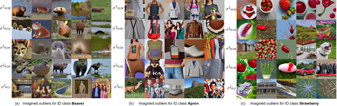
Figure 32: Visualization of the imageined outliers for the beaver, apron, strawberry class with different variance values $\sigma^{2}$.

31.4 Visualization of Outlier Generation by Embedding Interpolation

We visualize the generated outlier images by interpolating token embeddings from different classes in Figure 33. The result shows that interpolating different class token embeddings tends to generate images that are still in-distribution rather than images with semantically mixed or novel concepts, which is aligned with the observations in liew2022magicmix. Therefore, regularizing the model using such images is not effective for OOD detection (Table 6).

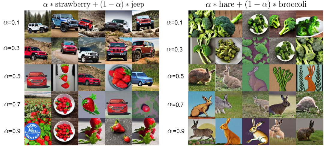
Figure 33: Visualization of the generated outlier images by interpolating token embeddings from different classes. We show the results with different interpolation weights $\alpha$.

31.5 Visualization of the Outlier Generation by Adding Noise

As in Table 6 in the main chapter, we visualize the generated outlier images by adding Gaussian and learnable noise to the token embeddings in Figure 34. We observe that adding Gaussian noise tends to generate either ID images or images that are far away from the given ID class. In addition, adding learnable noise to the token embeddings will generate images that completely deviate from the ID data. Both of them are less effective in regularizing the model’s decision boundary.

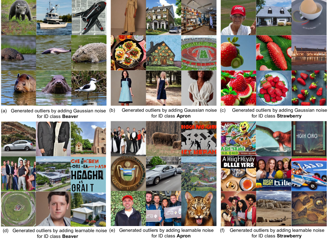
Figure 34: Visualization of the generated outlier images by adding Gaussian and learnable noise to the token embeddings from different classes.

31.6 Comparison with Training w/ real Outlier Data.

We compare with training using real outlier data on Cifar-100, i.e., 300K Random Images (Hendrycks et al., 2019), which contains 300K preprocessed images that do not belong to Cifar-100 classes. The result shows that Dream-ood (FPR95: 40.31%, AUROC: 90.15%) can match or even outperform outlier exposure with real OOD images (FPR95: 54.32%, AUROC: 91.34%) under the same training configuration while using fewer synthetic OOD images for OOD regularization (100K in total).

31.7 Visualization of Generated Inlier Images

We show in Figure 35 the visual comparison among the original Imagenet images, the generated images by our Dream-id, and the generated ID images using generic prompts "A high-quality photo of a [cls]" where "[cls]" denotes the class name. Interestingly, we observe that the prompt-based generation produces object-centric and distributionally dissimilar images from the original dataset. In contrast, our approach Dream-id generates inlier images that can resemble the original ID data, which helps model generalization.

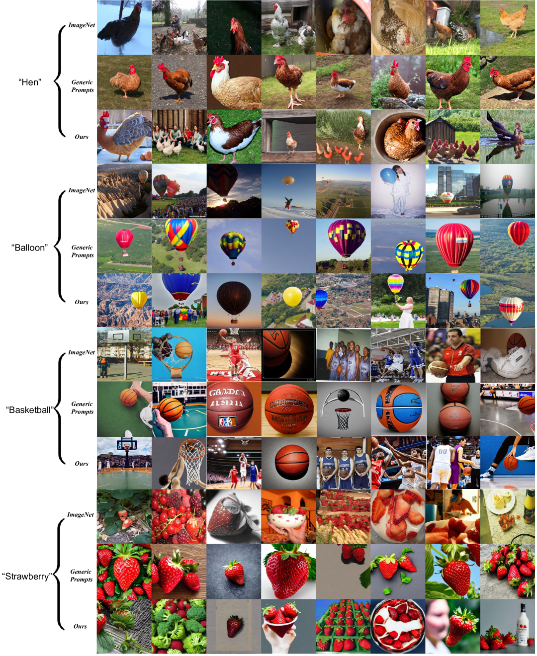
Figure 35: Visual comparison between our Dream-id vs. prompt-based image generation on four different classes.

31.8 Experimental Details for Model Generalization

We provide experimental details for Section 11.3 in the main chapter. We use ResNet-34 (He et al., 2016a) as the network architecture, trained with the standard cross-entropy loss. For both the Cifar-100 and Imagenet-100 datasets, we train the model for 100 epochs, using stochastic gradient descent with the cosine learning rate decay schedule, a momentum of 0.9, and a weight decay of $5e^{-4}$. The initial learning rate is set to 0.1 and the batch size is set to 160. We generate $1,000$ new ID samples per class using Stable Diffusion v1.4, which result in $100,000$ synthetic images. For both the baselines and our method, we train on a combination of the original Imagenet/Cifar samples and synthesized ones. To learn the feature encoder $h_{\theta}$, we set the temperature $t$ in Equation (17) to 0.1. Extensive ablations on hyperparameters $\sigma$ and $k$ are provided in Appendix 31.10.

31.9 Implementation Details of Baselines for Model Generalization

For a fair comparison, we implement all the data augmentation baselines by appending the original Imagenet-100 dataset with the same amount of augmented images (i.e., 100k) generated from different augmentation techniques. We follow the default hyperparameter setting as in their original papers.

• For RandAugment (Cubuk et al., 2020), we set the number of augmentation transformations to apply sequentially to 2. The magnitude for all the transformations is set to 9.

• For AutoAugment (Cubuk et al., 2019), we set the augmentation policy as the best one searched on ImageNet.

• For CutMix (yun2019cutmix), we use a CutMix probability of 1.0 and set $\beta$ in the Beta distribution to 1.0 for the label mixup.

• For AugMix (Hendrycks* et al., 2020), we randomly sample 3 augmentation chains and set $\alpha=1$ for the Dirichlet distribution to mix the images.

• For DeepAugment (Hendrycks et al., 2021a), we directly use the corrupted images for data augmentation provided in their Github repo .

• For MEMO (zhang2021memo), we follow the original paper and use the marginal entropy objective for test-time adaptation, which disentangles two distinct self-supervised learning signals: encouraging invariant predictions across different augmentations of the test point and encouraging confidence via entropy minimization.

Methods	ImageNet	ImageNet-A	ImageNet-v2
Original (no aug)	87.28	8.69	77.80
RandAugment	87.56	11.07	79.20
AutoAugment	87.40	10.37	79.00
CutMix	87.64	11.33	79.70
AugMix	87.22	9.39	77.80
Dream-id (Ours)	88.46$\pm$0.1	12.13$\pm$0.1	80.40$\pm$0.1

Table 25: Model generalization performance (accuracy, in %), using ImageNet-100 as the training data. The baselines are implemented by directly applying the augmentations on ImageNet-100.

We also provide the comparison in Table 25 with baselines that are directly trained by applying the augmentations on Imagenet without appending the original images. The model trained with the images generated by Dream-id can still outperform all the baselines by a considerable margin.

31.10 Ablation Studies on Model Generalization

In this section, we provide additional analysis of the hyperparameters and designs of Dream-id for ID generation and data augmentation. For all the ablations, we use the Imagenet-100 dataset as the in-distribution training data.

Ablation on the variance value $\sigma^{2}$.

We show in Table 26 the effect of $\sigma^{2}$ — the number of the variance value for the Gaussian kernel (Section 10.2). We vary $\sigma^{2}\in\{0.005,0.01,0.02,0.03\}$. A small-mild variance value $\sigma^{2}$ is more beneficial for model generalization.

$\sigma^{2}$	Imagenet	Imagenet-A	Imagenet-v2
0.005	87.62	11.39	78.50
0.01	88.46	12.13	80.40
0.02	87.72	10.85	77.70
0.03	87.28	10.91	78.20

Table 26: Ablation study on the variance value $\sigma^{2}$ in the Gaussian kernel for model generalization.

Ablation on $k$ in calculating $k$-NN distance.

In Table 27, we analyze the effect of $k$, i.e., the number of nearest neighbors for non-parametric sampling in the latent space. In particular, we vary $k=\{100,200,300,400,500\}$. We observe that our method is not sensitive to this hyperparameter, as $k$ varies from 100 to 500.

$k$	Imagenet	Imagenet-A	Imagenet-v2
100	88.51	12.11	79.92
200	88.35	12.04	80.01
300	88.46	12.13	80.40
400	88.43	12.01	80.12
500	87.72	11.78	80.29

Table 27: Ablation study on the $k$ for $k$-NN distance for model generalization.

31.11 Computational Cost

We summarize the computational cost of Dream-ood and different baselines on Imagenet-100 as follows. The post hoc OOD detection methods require training a classification model on the ID data ($\sim$8.2 h). The outlier synthesis baselines, such as VOS ($\sim$8.2 h), NPOS ($\sim$8.4 h), and GAN ($\sim$13.4 h) incorporate the training-time regularization with the synthetic outliers. Our Dream-ood involves learning the text-conditioned latent space ($\sim$8.2 h), image generation with diffusion models ($\sim$10.1 h for 100K images), and training with the generated outliers ($\sim$8.5 h).

31.12 Software and hardware

We run all experiments with Python 3.8.5 and PyTorch 1.13.1, using NVIDIA GeForce RTX 2080Ti GPUs.

32 SIREN: Shaping Representations for Detecting Out-of-Distribution Objects

32.1 Experimental Details

Following (Du et al., 2022c), we summarize the OOD detection evaluation task in Table 28. The OOD test dataset is selected from ms-coco and OpenImages dataset, which contains disjoint labels from the respective ID dataset. Siren is trained for a total of 50 epochs on pascal-voc, and trained for 30 epochs on bdd100k using ADAM optimizer. The initial learning rate is 2e-4 and decays at epoch 40 and 24 by 0.1 for pascal-voc and bdd100k dataset, respectively. We set the number of the object queries as 300, the batch size as 8, and the weight $\beta$ in Equation (30) as $1.5$. See detailed ablations on the hyperparameters on a validation OOD dataset in Appendix 32.3.

	Task 1	Task 2
ID train dataset	voc train	bdd train
ID val dataset	voc val	bdd val
OOD dataset	coco & OpenImages val	coco and OpenImages val
$\#$ID train images	16,551	69,853
$\#$ID val images	4,952	10,000
$\#$OOD images for coco	930	1,880
$\#$OOD images for OpenImages	1,761	1,761

Table 28: OOD detection evaluation tasks.

32.2 Estimating $\widehat{\kappa}$

We provide the mathematical details for the estimation of $\kappa$ in Equation (35). Concretely, we frame the estimation problem as deriving maximum likelihood estimators (MLEs) for the vMF density function, given the training data $\left\{\mathbf{r}_{i}\right\}_{i=1}^{M}$. Specifically, the maximum likelihood learning can be written as the following optimization problem:

$$\max_{\boldsymbol{\mu},{\kappa}}\mathcal{L}_{\textrm{MLE}}(\boldsymbol{\mu},\kappa)=\sum_{i=1}^{M}\log p\left(\mathbf{r}_{i}\right)=M\kappa\boldsymbol{\mu}^{\top}\overline{\mathbf{r}}+M\log Z_{d}(\kappa)$$ (58)

$$\text{ s.t. }\|\boldsymbol{\mu}\|=1\text{ and }\kappa\geq 0,$$

where $\overline{\mathbf{r}}=\frac{1}{M}\sum_{i=1}^{M}\mathbf{r}_{i}$ and $\mathcal{L}_{\textrm{MLE}}$ is the optimization objective of the maximum likelihood estimation for the distributional parameters $\boldsymbol{\mu},\kappa$. In order to optimize this objective, we take the derivatives of the objective w.r.t. the parameters $\boldsymbol{\mu},\kappa$ and set them to 0. Then, the optimal parameters $\boldsymbol{\mu}^{*},\widehat{\kappa}$ should satisfy the following two conditions:

$$\boldsymbol{\mu}^{*}=\frac{\overline{\mathbf{r}}}{\|\overline{\mathbf{r}}\|},\quad\frac{Z_{d}^{\prime}\left(\widehat{\kappa}\right)}{Z_{d}\left(\widehat{\kappa}\right)}=-\|\overline{\mathbf{r}}\|,$$ (59)

where $Z_{d}^{\prime}\left(\widehat{\kappa}\right)=\frac{dZ_{d}(\widehat{\kappa})}{d\widehat{\kappa}}$.

For the second condition in Equation (59), we let $\xi=(2\pi)^{d/2}$ and $s=d/2-1$ for notation simplicity. Put them into the Equation (57), we get the following:

$$Z_{d}(\widehat{\kappa})=\frac{\widehat{\kappa}^{s}}{\xi\cdot I_{s}(\widehat{\kappa})},\quad Z_{d}^{\prime}(\widehat{\kappa})=\frac{1}{\xi}\cdot\frac{s\widehat{\kappa}^{s-1}I_{s}(\widehat{\kappa})-\widehat{\kappa}^{s}I_{s}^{\prime}(\widehat{\kappa})}{I_{s}(\widehat{\kappa})^{2}}.$$ (60)

Divide $Z_{d}(\widehat{\kappa})$ by $Z_{d}^{\prime}(\widehat{\kappa})$, we get:

$$\frac{Z_{d}^{\prime}(\widehat{\kappa})}{Z_{d}(\widehat{\kappa})}=\frac{s}{\widehat{\kappa}}-\frac{I_{s}^{\prime}(\widehat{\kappa})}{I_{s}(\widehat{\kappa})}.$$ (61)

Note that the Bessel function holds a recursive property, which is given as follows:

$$\frac{I_{s}^{\prime}(\widehat{\kappa})}{I_{s}(\widehat{\kappa})}=\frac{s}{\widehat{\kappa}}+\frac{I_{s+1}^{\prime}(\widehat{\kappa})}{I_{s}(\widehat{\kappa})}.$$ (62)

Substitute $\frac{I_{s}^{\prime}(\widehat{\kappa})}{I_{s}(\widehat{\kappa})}$ in Equation (61) with the formula in Equation (62) and integrate it with the second condition of Equation (59), we get:

$$\frac{I_{d/2}(\widehat{\kappa})}{I_{d/2-1}(\widehat{\kappa})}=\|\overline{\mathbf{r}}\|.$$ (63)

Since there is no known closed-form solution to the Bessel ratio inversion problem as shown in the formula above, we adopt the approximation schemes based on the continued fraction form of the Bessel ratio function (Banerjee et al., 2005), namely:

$$R:=\frac{I_{d/2}(\widehat{\kappa})}{I_{d/2-1}(\widehat{\kappa})}=\frac{1}{\frac{d}{\widehat{\kappa}}+\frac{1}{\frac{d+2}{\widehat{\kappa}}+\cdots}}\approx\frac{1}{\frac{d}{\widehat{\kappa}}+R}.$$ (64)

Replace $R$ with $\|\overline{\mathbf{r}}\|$, we get $\widehat{\kappa}\approx\frac{d\cdot\|\overline{\mathbf{r}}\|}{1-\|\overline{\mathbf{r}}\|^{2}}$. Following (Banerjee et al., 2005), we further add a correction term $-\|\overline{\mathbf{r}}\|^{3}$ to the numerator and we get the approximated estimation calculated as:

$$\widehat{\kappa}=\frac{\|\mathbf{\overline{r}}\|(d-\|\mathbf{\overline{r}}\|^{2})}{1-\|\mathbf{\overline{r}}\|^{2}}.$$ (65)

32.3 Hyperparameter Analysis

Below we perform sensitivity analysis for each important hyperparameter. Our sensitivity analysis uses the speckle-noised pascal-voc validation dataset as OOD data, which is different from the actual OOD test datasets in use. We use Siren pre-trained with DINO (Caron et al., 2021) as the object detection backbone, trained on in-distribution dataset pascal-voc. We use the KNN score as the OOD score during inference.

Effect of the hypersphere dimension $d$. Siren projects the object feature embeddings into a lower-dimensional hypersphere in $\mathbb{R}^{d}$, which allows tractable vMF estimation. A reasonable choice of the hyperspherical dimension $d$ is able to preserve sufficient information for OOD detection while avoiding distributional parameter estimation in the high-dimension space. As shown in Table 29, using a dimension $d$ between 16 and 64 yields a desirable and stable performance on the OOD validation data while properly maintaining the ID performance (mAP). We set $d=16$ for pascal-voc and 64 for bdd100k in Table 1.

$d$	mAP$\uparrow$	FPR95 $\downarrow$	AUROC$\uparrow$
8	60.4	76.31	64.95
16	60.8	69.29	73.45
32	58.1	75.53	70.32
64	58.7	74.55	69.47
80	58.2	69.09	72.29

Table 29: Ablation study on the dimension of the hypersphere $d$.

Effect of the Siren loss weight $\beta$. In Table 30, we show the sensitivity of the OOD detection performance of our Siren w.r.t. the weight $\beta$ of the representation shaping loss. Overall, we find that $\beta=1.5$ achieves the best OOD detection and ID performance.

Effect of the $k$ in the KNN score. In Table 31, we show the sensitivity of the OOD detection performance of our Siren w.r.t. the $k$ of the KNN distance during inference. Overall, we find that $k=10$ achieves the best OOD detection performance.

$\beta$	mAP$\uparrow$	FPR95 $\downarrow$	AUROC$\uparrow$
0.1	60.2	69.72	73.21
0.5	59.2	71.09	72.36
1.0	59.8	76.20	70.49
1.5	60.8	69.29	73.45
2.0	58.9	70.41	71.22
2.5	56.0	77.20	68.37

Table 30: Ablation study on the loss weight $\beta$ for $\mathcal{L}_{\textsc{Siren}}$.

$k$	mAP$\uparrow$	FPR95 $\downarrow$	AUROC$\uparrow$
1	60.8	70.42	72.11
5	60.8	71.66	72.74
10	60.8	69.29	73.45
20	60.8	70.03	72.95
50	60.8	71.85	72.08
100	60.8	73.73	71.28
200	60.8	75.96	70.41

Table 31: Ablation study on the $k$ for the KNN distance.

32.4 Baselines

To evaluate the baselines, we follow the original methods in MSP (Hendrycks and Gimpel, 2017), ODIN (liang2018enhancing), KNN sun2022knn, and CSI (tack2020csi) and apply them accordingly on the classification branch of the object detectors. The Mahalanobis distance (lee2018simple) and gram matrices (DBLP:conf/icml/SastryO20) are calculated based on the penultimate-layer features of the decoder in ddetr. For CSI (tack2020csi), we use the rotation degree prediction (0${}^{\circ}$, 90${}^{\circ}$, 180${}^{\circ}$, 270${}^{\circ}$) as the self-supervised task. We set the temperature in the contrastive loss to 0.5. We use the penultimate-layer features of the decoder (with dimensionality 256) to perform contrastive learning. The weights of the losses that are used for classifying shifted instances and instance discrimination are both set to 1 following the original paper (tack2020csi). For OW-DETR (Gupta et al., 2022), we follow the original paper and utilize the sigmoid probability of the additional unknown class for OOD detection. For VOS (Du et al., 2022c), we use the same hyperparameters as those in the original paper and synthesize virtual outliers in the penultimate layer of the object detector. Then we regard the virtual outliers as the negative samples during the object classification. For Dismax (dismax), we add the dismax loss with learnable prototypes in the penultimate layer of ddter and apply the same inference score as the original paper for OOD detection.

32.5 Comparison of Training Time

We provide the comparison of the training time for various baselines in Table 32 on our reported hardware (Section 33.30 in the Appendix). As the table shows, the training of our method Siren incurs minimal computational overhead compared to the vanilla ddetr. In contrast, other baselines such as OW-DETR can be more than $2$ times slower than Siren.

Method	Training time (h)
ID: pascal-voc / bdd100k
Mahalanobis (lee2018simple)	9.7 / 27
Gram matrices (DBLP:conf/icml/SastryO20)	9.7 / 27
KNN (sun2022out)	9.7 / 27
CSI (tack2020csi)	17.1 / 47.9
VOS (Du et al., 2022c)	11.4 / 32.7
OW-DETR (Gupta et al., 2022)	23.7 / 59.3
Dismax (dismax)	10.0 / 27.7
Siren (ours)	10.1 / 27.7

Table 32: Comparison of the training time for different baselines in Table 1 of the main chapter.

32.6 Details of Visualization

For Figure 19 in the main chapter, we generate the toy data in the unit hypersphere by sampling from three vMF distributions in the 3D space. We adopt a concentration parameter $\kappa$ of 100 for all three classes. The centroid vectors are set to $[0,0,1],[\frac{\sqrt{3}}{2},0,-\frac{1}{2}]$ and $[-\frac{\sqrt{3}}{2},0,-\frac{1}{2}]$, respectively. The uncertainty surface is obtained by calculating the uncertainty score of $200^{2}$ points in the surface of the 3D ball.

32.7 Software and Hardware

We run all experiments with Python 3.8.5 and PyTorch 1.7.0, using 8 NVIDIA GeForce RTX 2080Ti GPUs.

33 How Does Unlabeled Data Provably Help Out-of-Distribution Detection?

33.1 Algorithm of SAL

We summarize our algorithm in implementation as follows.

Input: In-distribution data $\mathcal{S}^{\text{in}}=\left\{\left(\mathbf{x}_{i},y_{i}\right)\right\}_{i=1}^{n}$. Unlabeled wild data $\mathcal{S}_{\text{wild}}=\left\{\tilde{\mathbf{x}}_{i}\right\}_{i=1}^{m}$. $K$-way classification model $\mathbf{h}_{\mathbf{w}}$ and OOD classifier $\mathbf{g}_{\boldsymbol{\theta}}$. Parameter spaces $\mathcal{W}$ and $\Theta$. Learning rate lr for $\mathbf{g}_{\boldsymbol{\theta}}$.

Output: Learned OOD classifier $\mathbf{g}_{\widehat{\boldsymbol{\theta}}_{T}}$.

# Filtering stage

1) Perform ERM: $\mathbf{w}_{\mathcal{S}^{\text{in}}}\in argmin_{\mathbf{w}\in\mathcal{W}}R_{\mathcal{S}^{\text{in}}}(\mathbf{h}_{\mathbf{w}})$.

2) Calculate the reference gradient as $\bar{\nabla}=\frac{1}{n}\sum_{(\mathbf{x}_{i},y_{i})\in\mathcal{S}^{\text{in}}}\nabla\ell(\mathbf{h}_{\mathbf{w}_{\mathcal{S}^{\text{in}}}}(\mathbf{x}_{i}),y_{i})$.

3) Calculate gradient on $\mathcal{S}_{\text{wild}}$ as $\nabla\ell(\mathbf{h}_{\mathbf{w}_{\mathcal{S}^{\text{in}}}}(\tilde{\mathbf{x}}_{i}),\widehat{y}_{\tilde{\mathbf{x}}_{i}})$ and calculate the gradient matrix $\mathbf{G}$.

4) Calculate the top singular vector $\mathbf{v}$ of $\mathbf{G}$ and the score $\tau_{i}=\left<\nabla\ell(\mathbf{h}_{\mathbf{w}_{\mathcal{S}^{\text{in}}}}\big{(}\tilde{\mathbf{x}}_{i}),\widehat{y}_{\tilde{\mathbf{x}}_{i}})-\bar{\nabla},\mathbf{v}\right>^{2}$.

5) Get the candidate outliers $\mathcal{S}_{T}=\{\tilde{\mathbf{x}}_{i}\in\mathcal{S}_{\text{wild}},\tau_{i}\geq T\}$.

# Training Stage

for epoch in epochs do

    6) Sample batches of data ${\mathcal{B}^{\text{in}},\mathcal{B}_{T}}$ from ID and candidate outliers ${\mathcal{S}^{\text{in}},\mathcal{S}_{T}}$.

    7) Calculate the binary classification loss $R_{\mathcal{B}^{\text{in}},\mathcal{B}_{T}}(\mathbf{g}_{\boldsymbol{\theta}})$.

    8) Update the parameter by $\widehat{\boldsymbol{\theta}}_{T}=\boldsymbol{\theta}-{lr}\cdot\nabla R_{\mathcal{B}^{\text{in}},\mathcal{B}_{T}}(\mathbf{g}_{\boldsymbol{\theta}})$.

end for

Algorithm 4 SAL: Separate And Learn

33.2 Notations, Definitions, Assumptions and Important Constants

Here we summarize the important notations and constants in Tables 33 and 34, restate necessary definitions and assumptions in Sections 33.4 and 33.5.

33.3 Notations

Please see Table 33 for detailed notations.

Table 33: Main notations and their descriptions.

Notation	Description
Spaces
$\mathcal{X}$, $\mathcal{Y}$	the input space and the label space.
$\mathcal{W}$, $\Theta$	the hypothesis spaces
Distributions
$\mathbb{P}_{\text{wild}}$, $\mathbb{P}_{{\text{in}}}$, $\mathbb{P}_{{\text{out}}}$	data distribution for wild data, labeled ID data and OOD data
$\mathbb{P}_{\mathcal{X}\mathcal{Y}}$	the joint data distribution for ID data.
Data and Models
$\mathbf{w}$, $\mathbf{x}$, $\mathbf{v}$	weight/input/the top-1 right singular vector of $G$
$\widehat{\nabla}$, $\tau$	the average gradients on labeled ID data, uncertainty score
$y$ and $y_{\text{b}}$	label for ID classification and binary label for OOD detection
$\widehat{y}_{\mathbf{x}}$	Predicted one-hot label for input $\mathbf{x}$
$\mathbf{h}_{\mathbf{w}}$ and $\mathbf{g}_{\boldsymbol{\theta}}$	predictor on labeled in-distribution and binary predictor for OOD detection
$\mathcal{S}_{{\text{wild}}}^{\text{in}}$, $\mathcal{S}_{{\text{wild}}}^{\text{out}}$	inliers and outliers in the wild dataset.
$\mathcal{S}^{\text{in}}$, $\mathcal{S}_{\text{wild}}$	labeled ID data and unlabeled wild data
$n$, $m$	size of $\mathcal{S}^{\text{in}}$, size of $\mathcal{S}_{\text{wild}}$
$T$	the filtering threshold
$\mathcal{S}_{T}$	wild data whose uncertainty score higher than threshold $T$
Distances
$r_{1}$ and $r_{2}$	the radius of the hypothesis spaces $\mathcal{W}$ and $\Theta$, respectively
$\|\cdot\|_{2}$	$\ell_{2}$ norm
Loss, Risk and Predictor
$\ell(\cdot,\cdot)$, $\ell_{\text{b}}(\cdot,\cdot)$	ID loss function, binary loss function
$R_{\mathcal{S}}(\mathbf{h}_{\mathbf{w}})$	the empirical risk w.r.t. predictor $\mathbf{h}_{\mathbf{w}}$ over data $\mathcal{S}$
$R_{\mathbb{P}_{\mathcal{X}\mathcal{Y}}}(\mathbf{h}_{\mathbf{w}})$	the risk w.r.t. predictor $\mathbf{h}_{\mathbf{w}}$ over joint distribution $\mathbb{P}_{\mathcal{X}\mathcal{Y}}$
$R_{\mathbb{P}_{\text{in}},\mathbb{P}_{\text{out}}}(\mathbf{g}_{{\boldsymbol{\theta}}})$	the risk defined in Eq. 47
${ERR}_{\text{in}},{ERR}_{\text{out}}$	the error rates of regarding ID as OOD and OOD as ID

33.4 Definitions

Definition 1 ($\beta$-smooth).

We say a loss function $\ell(\mathbf{h}_{\mathbf{w}}(\mathbf{x}),y)$ (defined over $\mathcal{X}\times\mathcal{Y}$) is $\beta$-smooth, if for any $\mathbf{x}\in\mathcal{X}$ and $y\in\mathcal{Y}$,

$$\big{\|}\nabla\ell(\mathbf{h}_{\mathbf{w}}(\mathbf{x}),y)-\nabla\ell(\mathbf{h}_{\mathbf{w}^{\prime}}(\mathbf{x}),y)\big{\|}_{2}\leq\beta\|\mathbf{w}-\mathbf{w}^{\prime}\|_{2}$$

    

Definition 2 (Gradient-based Distribution Discrepancy).

Given distributions $\mathbb{P}$ and $\mathbb{Q}$ defined over $\mathcal{X}$, the Gradient-based Distribution Discrepancy w.r.t. predictor $\mathbf{h}_{\mathbf{w}}$ and loss $\ell$ is

$$d_{\mathbf{w}}^{\ell}(\mathbb{P},\mathbb{Q})=\big{\|}\nabla R_{\mathbb{P}}(\mathbf{h}_{\mathbf{w}},\widehat{\mathbf{h}})-\nabla R_{\mathbb{Q}}(\mathbf{h}_{\mathbf{w}},\widehat{\mathbf{h}})\big{\|}_{2},$$ (66)

where $\widehat{\mathbf{h}}$ is a classifier which returns the closest one-hot vector of $\mathbf{h}_{\mathbf{w}}$, $R_{\mathbb{P}}(\mathbf{h}_{\mathbf{w}},\widehat{\mathbf{h}})=\mathbb{E}_{\mathbf{x}\sim\mathbb{P}}\ell(\mathbf{h}_{\mathbf{w}},\widehat{\mathbf{h}})$ and $R_{\mathbb{Q}}(\mathbf{h}_{\mathbf{w}},\widehat{\mathbf{h}})=\mathbb{E}_{\mathbf{x}\sim\mathbb{Q}}\ell(\mathbf{h}_{\mathbf{w}},\widehat{\mathbf{h}})$.

Definition 3 ($(\gamma,\zeta)$-discrepancy).

We say a wild distribution $\mathbb{P}_{\text{wild}}$ has $(\gamma,\zeta)$-discrepancy w.r.t. an ID joint distribution $\mathbb{P}_{\text{in}}$, if $\gamma>\min_{\mathbf{w}\in\mathcal{W}}R_{\mathbb{P}_{\mathcal{X}\mathcal{Y}}}(\mathbf{h}_{\mathbf{w}})$, and for any parameter $\mathbf{w}\in\mathcal{W}$ satisfying that $R_{\mathbb{P}_{\mathcal{X}\mathcal{Y}}}(\mathbf{h}_{\mathbf{w}})\leq\gamma$ should meet the following condition

$$d_{\mathbf{w}}^{\ell}(\mathbb{P}_{\text{in}},\mathbb{P}_{\text{wild}})>\zeta,$$

where $R_{\mathbb{P}_{\mathcal{X}\mathcal{Y}}}(\mathbf{h}_{\mathbf{w}})=\mathbb{E}_{(\mathbf{x},y)\sim\mathbb{P}_{\mathcal{X}\mathcal{Y}}}\ell(\mathbf{h}_{\mathbf{w}}(\mathbf{x}),y)$.

In Section 33.18, we empirically calculate the values of the distribution discrepancy between the ID joint distribution $\mathbb{P}_{\mathcal{X}\mathcal{Y}}$ and the wild distribution $\mathbb{P}_{\text{wild}}$.    

33.5 Assumptions

Assumption 1.

    

• The parameter space $\mathcal{W}\subset B(\mathbf{w}_{0},r_{1})\subset\mathbb{R}^{d}$ ($\ell_{2}$ ball of radius $r_{1}$ around $\mathbf{w}_{0}$);

• The parameter space $\Theta\subset B(\boldsymbol{\theta}_{0},r_{2})\subset\mathbb{R}^{d^{\prime}}$ ($\ell_{2}$ ball of radius $r_{2}$ around $\boldsymbol{\theta}_{0}$);

• $\ell(\mathbf{h}_{\mathbf{w}}(\mathbf{x}),y)\geq 0$ and $\ell(\mathbf{h}_{\mathbf{w}}(\mathbf{x}),y)$ is $\beta_{1}$-smooth;

• $\ell_{\text{b}}(\mathbf{g}_{\boldsymbol{\theta}}(\mathbf{x}),y_{\text{b}})\geq 0$ and $\ell_{\text{b}}(\mathbf{g}_{\boldsymbol{\theta}}(\mathbf{x}),y_{\text{b}})$ is $\beta_{2}$-smooth;

• $\sup_{(\mathbf{x},y)\in\mathcal{X}\times\mathcal{Y}}\|\nabla\ell(\mathbf{h}_{\mathbf{w}_{0}}(\mathbf{x}),y)\|_{2}=b_{1}$, $\sup_{(\mathbf{x},y_{\text{b}})\in\mathcal{X}\times\mathcal{Y}_{\text{b}}}\|\nabla\ell(\mathbf{g}_{\boldsymbol{\theta}_{0}}(\mathbf{x}),y_{\text{b}})\|_{2}=b_{2}$;

• $\sup_{(\mathbf{x},y)\in\mathcal{X}\times\mathcal{Y}}\ell(\mathbf{h}_{\mathbf{w}_{0}}(\mathbf{x}),y)=B_{1}$, $\sup_{(\mathbf{x},y_{\text{b}})\in\mathcal{X}\times\mathcal{Y}_{\text{b}}}\ell(\mathbf{g}_{\boldsymbol{\theta}_{0}}(\mathbf{x}),y_{\text{b}})=B_{2}$.

Remark 2.

For neural networks with smooth activation functions and softmax output function, we can check that the norm of the second derivative of the loss functions (cross-entropy loss and sigmoid loss) is bounded given the bounded parameter space, which implies that the $\beta$-smoothness of the loss functions can hold true. Therefore, our assumptions are reasonable in practice.

Assumption 2.

$\ell(\mathbf{h}(\mathbf{x}),\widehat{y}_{\mathbf{x}})\leq\min_{y\in\mathcal{Y}}\ell(\mathbf{h}(\mathbf{x}),{y}),$ where $\widehat{y}_{\mathbf{x}}$ returns the closest one-hot label of the predictor $\mathbf{h}$’s output on $\mathbf{x}$.

Remark 3.

The assumption means the loss incurred by using the predicted labels given by the classifier itself is smaller or equal to the loss incurred by using any label in the label space. If $y=\widehat{y}_{\mathbf{x}}$, the assumption is satisfied obviously. If $y\neq\widehat{y}_{\mathbf{x}}$, then we provide two examples to illustrate the validity of the assumption. For example, (1) if the loss $\ell$ is the cross entropy loss, let $K=2,\mathbf{h}(\mathbf{x})=[h_{1},h_{2}]$ (classification output after softmax) and $h_{1}>h_{2}$. Therefore, we have $\widehat{y}_{\mathbf{x}}=0$. Suppose $y=1$, we can get $\ell(\mathbf{h}(\mathbf{x}),\widehat{y}_{\mathbf{x}})=-\operatorname{log}(h_{1})<\ell(\mathbf{h}(\mathbf{x}),y)=-\operatorname{log}(h_{2})$. (2) If $\ell$ is the hinge loss for binary classification, thus we have $K=1$, let $\mathbf{h}(\mathbf{x})=h_{1}<0$ and thus $\widehat{y}_{\mathbf{x}}=-1$. Suppose $y=1$, we can get $\ell(\mathbf{h}(\mathbf{x}),\widehat{y}_{\mathbf{x}})=\operatorname{max}(0,1+h_{1})<\operatorname{max}(0,1-h_{1})=\ell(\mathbf{h}(\mathbf{x}),y).$

33.6 Constants in Theory

Table 34: Constants in theory.

Constants	Description
$M=\beta_{1}r_{1}^{2}+b_{1}r_{1}+B_{1}$	the upper bound of loss $\ell(\mathbf{h}_{\mathbf{w}}(\mathbf{x}),y)$, see Proposition 1
$M^{\prime}=2(\beta_{1}r_{1}+b_{1})^{2}$	the upper bound of filtering score $\tau$
$\tilde{M}=\beta_{1}M$	a constant for simplified representation
$L=\beta_{2}r_{2}^{2}+b_{2}r_{2}+B_{2}$	the upper bound of loss $\ell_{\text{b}}(\mathbf{g}_{\boldsymbol{\theta}}(\mathbf{x}),y_{\text{b}})$, see Proposition 1
$d$, $d^{\prime}$	the dimensions of parameter spaces $\mathcal{W}$ and $\Theta$, respectively
$R^{*}_{{\text{in}}}$	the optimal ID risk, i.e., $R^{*}_{{\text{in}}}=\min_{\mathbf{w}\in\mathcal{W}}\mathbb{E}_{(\mathbf{x},y)\sim\mathbb{P}_{\mathcal{X}\mathcal{Y}}}\ell(\mathbf{h}_{\mathbf{w}}(\mathbf{x}),y)$
$\delta(T)$	the main error in Eq. 43
$\zeta$	the discrepancy between $\mathbb{P}_{\text{in}}$ and $\mathbb{P}_{\text{wild}}$
$\pi$	the ratio of OOD distribution in $\mathbb{P}_{\text{wild}}$

33.7 Main Theorems

In this section, we provide a detailed and formal version of our main theorems with a complete description of the constant terms and other additional details that are omitted in the main paper.

Theorem 1.

If Assumptions 1 and 2 hold, $\mathbb{P}_{\text{wild}}$ has $(\gamma,\zeta)$-discrepancy w.r.t. $\mathbb{P}_{\mathcal{X}\mathcal{Y}}$, and there exists $\eta\in(0,1)$ s.t. $\Delta=(1-\eta)^{2}\zeta^{2}-8\beta_{1}R_{{\text{in}}}^{*}>0$, then for

$$n=\Omega\big{(}\frac{\tilde{M}+M(r_{1}+1)d}{\eta^{2}\Delta}+\frac{M^{2}{d}}{(\gamma-R_{\text{in}}^{*})^{2}}\big{)},~~~~~m=\Omega\big{(}\frac{\tilde{M}+M(r_{1}+1)d}{\eta^{2}\zeta^{2}}\big{)},$$

with the probability at least $9/10$, for any $0<T<M^{\prime}$ $($here $M^{\prime}=2(\beta_{1}r_{1}+b_{1})^{2}$ is the upper bound of filtering score $\tau_{i}$, i.e., $\tau_{i}\leq M^{\prime}$$)$,

$${ERR}_{\text{in}}\leq\frac{8\beta_{1}}{T}R_{\text{in}}^{*}+O\Big{(}\frac{\tilde{M}}{T}\sqrt{\frac{d}{n}}\Big{)}+O\Big{(}\frac{\tilde{M}}{T}\sqrt{\frac{d}{(1-\pi)m}}\Big{)},$$ (67)

$$\begin{split}{ERR}_{\text{out}}&\leq\delta(T)+O\Big{(}\frac{\tilde{M}}{1-T/M^{\prime}}\sqrt{\frac{d}{{\pi}^{2}n}}\Big{)}\\ &+O\Big{(}\frac{\max\{{\tilde{M}\sqrt{d}},\Delta_{\zeta}^{\eta}/\pi\}}{1-T/M^{\prime}}\sqrt{\frac{1}{{\pi}^{2}(1-\pi)m}}\Big{)},\end{split}$$ (68)

where $R^{*}_{{\text{in}}}$ is the optimal ID risk, i.e., $R^{*}_{{\text{in}}}=\min_{\mathbf{w}\in\mathcal{W}}\mathbb{E}_{(\mathbf{x},y)\sim\mathbb{P}_{\mathcal{X}\mathcal{Y}}}\ell(\mathbf{h}_{\mathbf{w}}(\mathbf{x}),y)$,

$$\begin{split}\delta(T)&=\frac{\max\{0,1-\Delta_{\zeta}^{\eta}/\pi\}}{(1-T/M^{\prime})},~~~\Delta_{\zeta}^{\eta}={0.98\eta^{2}\zeta^{2}}-8\beta_{1}R_{\text{in}}^{*},\\ &M=\beta_{1}r_{1}^{2}+b_{1}r_{1}+B_{1},~~~\tilde{M}=M\beta_{1},\end{split}$$ (69)

and $d$ is the dimension of the parameter space $\mathcal{W}$, here $\beta_{1},r_{1},B_{1}$ are given in Assumption 1.

    

      

Theorem 2.

1) If $\Delta_{\zeta}^{\eta}\geq(1-\epsilon)\pi$ for a small error $\epsilon\geq 0$, then the main error $\delta(T)$ defined in Eq. 44 satisfies that

$$\delta(T)\leq\frac{\epsilon}{1-T/{M^{\prime}}}.$$

2) If $\zeta\geq 2.011\sqrt{8\beta_{1}R_{\text{in}}^{*}}+1.011\sqrt{\pi}$, then there exists $\eta\in(0,1)$ ensuring that $\Delta>0$ and $\Delta_{\zeta}^{\eta}>\pi$ hold, which implies that the main error $\delta(T)=0$.

    

      

Theorem 3.

Given the same conditions in Theorem 8.1, if we further require that

$$n=\Omega\Big{(}\frac{\tilde{M}^{2}d}{\min\{\pi,\Delta_{\zeta}^{\eta}\}^{2}}\Big{)},~~~m=\Omega\Big{(}\frac{\tilde{M}^{2}d+\Delta_{\zeta}^{\eta}}{\pi^{2}(1-\pi)\min\{\pi,\Delta_{\zeta}^{\eta}\}^{2}}\Big{)},$$

then with the probability at least $89/100$, for any $0<T<0.9M^{\prime}\min\{1,\Delta_{\zeta}^{\eta}/\pi\}$, the OOD classifier $\mathbf{g}_{\widehat{\boldsymbol{\theta}}_{T}}$ learned by the proposed algorithm satisfies the following risk estimation

$$R_{\mathbb{P}_{\text{in}},\mathbb{P}_{\text{out}}}(\mathbf{g}_{\widehat{\boldsymbol{\theta}}_{T}})\leq\inf_{\boldsymbol{\theta}\in\Theta}R_{\mathbb{P}_{\text{in}},\mathbb{P}_{\text{out}}}(\mathbf{g}_{{\boldsymbol{\theta}}})+\frac{3.5L}{1-\delta(T)}\delta({T})+\frac{9(1-\pi)L\beta_{1}}{\pi(1-\delta(T))T}R_{\text{in}}^{*}$$ (70)

$$+ O\Big{(}\frac{L\max\{\tilde{M}\sqrt{d},\sqrt{d^{\prime}}\}}{\min\{\pi,\Delta_{\zeta}^{\eta}\}T^{\prime}}\sqrt{\frac{1}{n}}\Big{)}+O\Big{(}\frac{L\max\{\tilde{M}\sqrt{d},\sqrt{d^{\prime}},\Delta_{\zeta}^{\eta}\}}{\min\{\pi,\Delta_{\zeta}^{\eta}\}T^{\prime}}\sqrt{\frac{1}{\pi^{2}(1-\pi)m}}\Big{)},$$

where $R_{\text{in}}^{*}$, $\Delta_{\zeta}^{\eta}$, $M$, $M^{\prime}$, $\tilde{M}$ and $d$ are shown in Theorem 8.1, $d^{\prime}$ is the dimension of space $\Theta$,

$$L=\beta_{2}r_{2}^{2}+b_{2}r_{2}+B_{2},~~~T^{\prime}=T/(1+T),$$

and the risk $R_{\mathbb{P}_{\text{in}},\mathbb{P}_{\text{out}}}(\mathbf{g}_{{\boldsymbol{\theta}}})$ is defined as follows:

$$R_{\mathbb{P}_{\text{in}},\mathbb{P}_{\text{out}}}(\mathbf{g}_{\widehat{\boldsymbol{\theta}}_{T}})=\mathbb{E}_{\mathbf{x}\sim\mathbb{P}_{\text{in}}}\ell_{\text{b}}(\mathbf{g}_{\boldsymbol{\theta}}(\mathbf{x}),y_{+})+\mathbb{E}_{\mathbf{x}\sim\mathbb{P}_{\text{out}}}\ell_{\text{b}}(\mathbf{g}_{\boldsymbol{\theta}}(\mathbf{x}),y_{-}).$$

    

      

Theorem 4.

Given the same conditions in Theorem 8.1, with the probability at least $9/10$,

$$\begin{split}\mathbb{E}_{\tilde{\mathbf{x}}_{i}\sim\mathcal{S}_{\text{wild}}^{\text{in}}}\tau_{i}\leq&8\beta_{1}R_{\text{in}}^{*}+O(\beta_{1}M\sqrt{\frac{d}{n}})+O(\beta_{1}M\sqrt{\frac{d}{(1-\pi)m}}),\end{split}$$

$$\begin{split}\mathbb{E}_{\tilde{\mathbf{x}}_{i}\sim\mathcal{S}_{\text{wild}}^{\text{out}}}\tau_{i}\geq&\frac{0.98\eta^{2}\zeta^{2}}{\pi}-\frac{8\beta_{1}R_{\text{in}}^{*}}{\pi}-\epsilon^{\prime}(n,m),\end{split}$$

furthermore, if the realizability assumption for ID distribution holds (understand_ml; Fang et al., 2022), then

$$\mathbb{E}_{\tilde{\mathbf{x}}_{i}\sim\mathcal{S}_{\text{wild}}^{\text{in}}}\tau_{i}\leq O(\beta_{1}M\sqrt{\frac{d}{n}})+O(\beta_{1}M\sqrt{\frac{d}{(1-\pi)m}})$$

$$\begin{split}\mathbb{E}_{\tilde{\mathbf{x}}_{i}\sim\mathcal{S}_{\text{wild}}^{\text{out}}}\tau_{i}\geq&\frac{0.98\eta^{2}\zeta^{2}}{\pi}-\epsilon^{\prime}(n,m),\end{split}$$

where

$$\epsilon^{\prime}(n,m)\leq O(\frac{\beta_{1}M}{\pi}\sqrt{\frac{d}{n}})+O\Big{(}({{\beta_{1}M\sqrt{d}}+\sqrt{1-\pi}\Delta_{\zeta}^{\eta}/\pi})\sqrt{\frac{1}{{\pi}^{2}(1-\pi)m}}\Big{)},$$

and $R_{\text{in}}^{*}$, $\Delta_{\zeta}^{\eta}$, $M$ and $d$ are shown in Theorem 8.1.

33.8 Proofs of Main Theorems

33.9 Proof of Theorem 8.1

Step 1. With the probability at least $1-\frac{7}{3}\delta>0$,

$$\begin{split}\mathbb{E}_{\tilde{\mathbf{x}}_{i}\sim\mathcal{S}_{\text{wild}}^{\text{in}}}\tau_{i}\leq&8\beta_{1}R_{\text{in}}^{*}\\ +&4\beta_{1}\Big{[}C\sqrt{\frac{Mr_{1}(\beta_{1}r_{1}+b_{1})d}{n}}+C\sqrt{\frac{Mr_{1}(\beta_{1}r_{1}+b_{1})d}{(1-\pi)m-\sqrt{m\log(6/\delta)/2}}}\\ &+3M\sqrt{\frac{2\log(6/\delta)}{n}}+M\sqrt{\frac{2\log(6/\delta)}{(1-\pi)m-\sqrt{m\log(6/\delta)/2}}}\Big{]},\end{split}$$

This can be proven by Lemma 12.7 and following inequality

$$\begin{split}&\mathbb{E}_{\tilde{\mathbf{x}}_{i}\sim\mathcal{S}_{\text{wild}}^{\text{in}}}\tau_{i}\leq\mathbb{E}_{\tilde{\mathbf{x}}_{i}\sim\mathcal{S}_{\text{wild}}^{\text{in}}}\big{\|}\nabla\ell(\mathbf{h}_{\mathbf{w}_{\mathcal{S}^{\text{in}}}}(\tilde{\mathbf{x}}_{i}),\widehat{\mathbf{h}}_{\mathbf{w}_{\mathcal{S}^{\text{in}}}}(\tilde{\mathbf{x}}_{i}))-\mathbb{E}_{(\mathbf{x}_{j},y_{j})\sim\mathcal{S}^{\operatorname{in}}}\nabla\ell(\mathbf{h}_{\mathbf{w}_{\mathcal{S}^{\text{in}}}}(\mathbf{x}_{j}),y_{j})\big{\|}_{2}^{2},\end{split}$$

Step 2. It is easy to check that

$$\mathbb{E}_{\tilde{\mathbf{x}}_{i}\sim\mathcal{S}_{\text{wild}}}\tau_{i}=\frac{|\mathcal{S}_{\text{wild}}^{\text{in}}|}{|\mathcal{S}_{\text{wild}}|}\mathbb{E}_{\tilde{\mathbf{x}}_{i}\sim\mathcal{S}_{\text{wild}}^{\text{in}}}\tau_{i}+\frac{|\mathcal{S}_{\text{wild}}^{\text{out}}|}{|\mathcal{S}_{\text{wild}}|}\mathbb{E}_{\tilde{\mathbf{x}}_{i}\sim\mathcal{S}_{\text{wild}}^{\text{out}}}\tau_{i}.$$

Step 3. Let

$$\begin{split}\epsilon(n,m)=&4\beta_{1}[C\sqrt{\frac{Mr_{1}(\beta_{1}r_{1}+b_{1})d}{n}}+C\sqrt{\frac{Mr_{1}(\beta_{1}r_{1}+b_{1})d}{(1-\pi)m-\sqrt{m\log(6/\delta)/2}}}\\ +&3M\sqrt{\frac{2\log(6/\delta)}{n}}+M\sqrt{\frac{2\log(6/\delta)}{(1-\pi)m-\sqrt{m\log(6/\delta)/2}}}].\end{split}$$

Under the condition in Theorem 5, with the probability at least $\frac{97}{100}-\frac{7}{3}\delta>0$,

$$\begin{split}\mathbb{E}_{\tilde{\mathbf{x}}_{i}\sim\mathcal{S}_{\text{wild}}^{\text{out}}}\tau_{i}\geq&\frac{m}{|\mathcal{S}_{\text{wild}}^{\text{out}}|}\big{[}\frac{98\eta^{2}\zeta^{2}}{100}-\frac{|\mathcal{S}_{\text{wild}}^{\text{in}}|}{m}8\beta_{1}R_{\text{in}}^{*}-\frac{|\mathcal{S}_{\text{wild}}^{\text{in}}|}{m}\epsilon(n,m)\big{]}\\ \geq&\frac{m}{|\mathcal{S}_{\text{wild}}^{\text{out}}|}\big{[}\frac{98\eta^{2}\zeta^{2}}{100}-8\beta_{1}R_{\text{in}}^{*}-\epsilon(n,m)\big{]}\\ \geq&\big{[}\frac{1}{\pi}-\frac{\sqrt{\log{6/\delta}}}{\pi^{2}\sqrt{2m}+\pi\sqrt{\log(6/\delta)}}\big{]}\big{[}\frac{98\eta^{2}\zeta^{2}}{100}-8\beta_{1}R_{\text{in}}^{*}-\epsilon(n,m)\big{]}.\end{split}$$

In this proof, we set

$$\Delta(n,m)=\big{[}\frac{1}{\pi}-\frac{\sqrt{\log{6/\delta}}}{\pi^{2}\sqrt{2m}+\pi\sqrt{\log(6/\delta)}}\big{]}\big{[}\frac{98\eta^{2}\zeta^{2}}{100}-8\beta_{1}R_{\text{in}}^{*}-\epsilon(n,m)\big{]}.$$

Note that $\Delta_{\zeta}^{\eta}={0.98\eta^{2}\zeta^{2}}-8\beta_{1}R_{\text{in}}^{*}$, then

$$\Delta(n,m)=\frac{1}{\pi}\Delta_{\zeta}^{\eta}-\frac{1}{\pi}\epsilon(n,m)-\Delta_{\zeta}^{\eta}\epsilon(m)+\epsilon(n)\epsilon(n,m),$$

where $\epsilon(m)={\sqrt{\log{6/\delta}}}/({\pi^{2}\sqrt{2m}+\pi\sqrt{\log(6/\delta)}})$.

Step 4. Under the condition in Theorem 5, with the probability at least $\frac{97}{100}-\frac{7}{3}\delta>0$,

$$\frac{|\{\tilde{\mathbf{x}}_{i}\in\mathcal{S}_{\operatorname{wild}}^{\operatorname{out}}:\tau_{i}\leq T\}|}{|\mathcal{S}_{\operatorname{wild}}^{\operatorname{out}}|}\leq\frac{1-\min\{1,\Delta(n,m)\}}{1-T/{M^{\prime}}},$$ (71)

and

$$\frac{|\{\tilde{\mathbf{x}}_{i}\in\mathcal{S}_{\operatorname{wild}}^{\operatorname{in}}:\tau_{i}>T\}|}{|\mathcal{S}_{\operatorname{wild}}^{\operatorname{in}}|}\leq\frac{8\beta_{1}R_{\text{in}}^{*}+\epsilon(n,m)}{T}.$$ (72)

We prove this step: let $Z$ be the uniform random variable with $\mathcal{S}_{\operatorname{wild}}^{\operatorname{out}}$ as its support and $Z(i)=\tau_{i}/(2(\beta_{1}r_{1}+b_{1})^{2})$, then by the Markov inequality, we have

$$\frac{|\{\tilde{\mathbf{x}}_{i}\in\mathcal{S}_{\operatorname{wild}}^{\operatorname{out}}:\tau_{i}>T\}|}{|\mathcal{S}_{\operatorname{wild}}^{\operatorname{out}}|}=P(Z(i)>T/(2(\beta_{1}r_{1}+b_{1})^{2}))\geq\frac{\Delta(n,m)-T/(2(\beta_{1}r_{1}+b_{1})^{2})}{1-T/(2(\beta_{1}r_{1}+b_{1})^{2})}.$$ (73)

Let $Z$ be the uniform random variable with $\mathcal{S}_{\operatorname{wild}}^{\operatorname{in}}$ as its support and $Z(i)=\tau_{i}$, then by the Markov inequality, we have

$$\frac{|\{\tilde{\mathbf{x}}_{i}\in\mathcal{S}_{\operatorname{wild}}^{\operatorname{in}}:\tau_{i}>T\}|}{|\mathcal{S}_{\operatorname{wild}}^{\operatorname{in}}|}=P(Z(i)>T)\leq\frac{\mathbb{E}[Z]}{T}=\frac{8\beta_{1}R_{\text{in}}^{*}+\epsilon(n,m)}{T}.$$ (74)

Step 5. If $\pi\leq\Delta_{\zeta}^{\eta}/(1-\epsilon/{M^{\prime}})$, then with the probability at least $\frac{97}{100}-\frac{7}{3}\delta>0$,

$$\frac{|\{\tilde{\mathbf{x}}_{i}\in\mathcal{S}_{\operatorname{wild}}^{\operatorname{out}}:\tau_{i}\leq T\}|}{|\mathcal{S}_{\operatorname{wild}}^{\operatorname{out}}|}\leq\frac{\epsilon+M^{\prime}\epsilon^{\prime}(n,m)}{M^{\prime}-T},$$ (75)

and

$$\frac{|\{\tilde{\mathbf{x}}_{i}\in\mathcal{S}_{\operatorname{wild}}^{\operatorname{in}}:\tau_{i}>T\}|}{|\mathcal{S}_{\operatorname{wild}}^{\operatorname{in}}|}\leq\frac{8\beta_{1}R_{\text{in}}^{*}+\epsilon(n,m)}{T},$$ (76)

where $\epsilon^{\prime}(n,m)={\epsilon(n,m)}/{\pi}+\Delta_{\zeta}^{\eta}\epsilon(m)-\epsilon(n)\epsilon(n,m)$.

Step 6. If we set $\delta=3/100$, then it is easy to see that

$$\begin{split}&\epsilon(m)\leq O(\frac{1}{\pi^{2}\sqrt{m}}),\\ &\epsilon(n,m)\leq O(\beta_{1}M\sqrt{\frac{d}{n}})+O(\beta_{1}M\sqrt{\frac{d}{(1-\pi)m}}),\\ &\epsilon^{\prime}(n,m)\leq O(\frac{\beta_{1}M}{\pi}\sqrt{\frac{d}{n}})+O\Big{(}({{\beta_{1}M\sqrt{d}}+\sqrt{1-\pi}\Delta_{\zeta}^{\eta}/\pi})\sqrt{\frac{1}{{\pi}^{2}(1-\pi)m}}\Big{)}.\end{split}$$

Step 7. By results in Steps 4, 5 and 6, We complete this proof.

33.10 Proof of Theorem 8.2

The first result is trivial. Hence, we omit it. We mainly focus on the second result in this theorem. In this proof, then we set

$$\eta={\sqrt{8\beta_{1}R_{\text{in}}^{*}+0.99\pi}}/({\sqrt{0.98}\sqrt{8\beta_{1}R_{\text{in}}^{*}}+\sqrt{8\beta_{1}R_{\text{in}}^{*}+\pi}})$$

Note that it is easy to check that

$$\zeta\geq 2.011\sqrt{8\beta_{1}R_{\text{in}}^{*}}+1.011\sqrt{\pi}\geq\sqrt{8\beta_{1}R_{\text{in}}^{*}}+1.011\sqrt{8\beta_{1}R_{\text{in}}^{*}+\pi}.$$

Therefore,

$$\eta\zeta\geq\frac{1}{\sqrt{0.98}}\sqrt{8\beta_{1}R_{\text{in}}^{*}+0.99\pi}>\sqrt{8\beta_{1}R_{\text{in}}^{*}+\pi},$$

which implies that $\Delta_{\zeta}^{\eta}>\pi$. Note that

$$\begin{split}(1-\eta)\zeta&\geq\frac{1}{\sqrt{0.98}}\big{(}{{\sqrt{0.98}\sqrt{8\beta_{1}R_{\text{in}}^{*}}+\sqrt{8\beta_{1}R_{\text{in}}^{*}+\pi}}-{\sqrt{8\beta_{1}R_{\text{in}}^{*}+0.99\pi}}}\big{)}>\sqrt{8\beta_{1}R_{\text{in}}^{*}},\end{split}$$

which implies that $\Delta>0$. We have completed this proof.  

33.11 Proof of Theorem 8.3

Let

$$\boldsymbol{\theta}^{*}\in\operatorname*{arg\,min}_{\boldsymbol{\theta}\in\Theta}R_{\mathbb{P}_{\text{in}},\mathbb{P}_{\text{out}}}(\boldsymbol{\theta}).$$

Then by Lemma 12.1 and Lemma 12.14, we obtain that with the high probability

$$\begin{split}&R_{\mathbb{P}_{\text{in}},\mathbb{P}_{\text{out}}}(\mathbf{g}_{\widehat{\boldsymbol{\theta}}_{T}})-R_{\mathbb{P}_{\text{in}},\mathbb{P}_{\text{out}}}(\mathbf{g}_{{\boldsymbol{\theta}}^{*}})\\ =&R_{\mathbb{P}_{\text{in}},\mathbb{P}_{\text{out}}}(\mathbf{g}_{\widehat{\boldsymbol{\theta}}_{T}})-R_{\mathcal{S}^{\text{in}},\mathcal{S}_{T}}(\mathbf{g}_{\widehat{\boldsymbol{\theta}}_{T}})+R_{\mathcal{S}^{\text{in}},\mathcal{S}_{T}}(\mathbf{g}_{\widehat{\boldsymbol{\theta}}_{T}})-R_{\mathcal{S}^{\text{in}},\mathcal{S}_{T}}(\mathbf{g}_{{\boldsymbol{\theta}}^{*}})\\ +&R_{\mathcal{S}^{\text{in}},\mathcal{S}_{T}}(\mathbf{g}_{{\boldsymbol{\theta}}^{*}})-R_{\mathbb{P}_{\text{in}},\mathbb{P}_{\text{out}}}(\mathbf{g}_{{\boldsymbol{\theta}}^{*}})\\ \leq&R_{\mathbb{P}_{\text{in}},\mathbb{P}_{\text{out}}}(\mathbf{g}_{\widehat{\boldsymbol{\theta}}_{T}})-R_{\mathcal{S}^{\text{in}},\mathcal{S}_{T}}(\mathbf{g}_{\widehat{\boldsymbol{\theta}}_{T}})\\ +&R_{\mathcal{S}^{\text{in}},\mathcal{S}_{T}}(\mathbf{g}_{{\boldsymbol{\theta}}^{*}})-R_{\mathbb{P}_{\text{in}},\mathbb{P}_{\text{out}}}(\mathbf{g}_{{\boldsymbol{\theta}}^{*}})\\ \leq&2\sup_{\boldsymbol{\theta}\in\Theta}\big{|}R_{\mathcal{S}^{\text{in}}}^{+}(\mathbf{g}_{{\boldsymbol{\theta}}})-R_{\mathbb{P}_{\text{in}}}^{+}(\mathbf{g}_{{\boldsymbol{\theta}}})\big{|}\\ +&\sup_{\boldsymbol{\theta}\in\Theta}\big{(}R_{\mathcal{S}^{\text{out}}}^{-}(\mathbf{g}_{{\boldsymbol{\theta}}})-R_{\mathbb{P}_{\text{out}}}^{-}(\mathbf{g}_{{\boldsymbol{\theta}}})\big{)}+\sup_{\boldsymbol{\theta}\in\Theta}\big{(}R_{\mathbb{P}_{\text{out}}}^{-}(\mathbf{g}_{{\boldsymbol{\theta}}})-R_{\mathcal{S}^{\text{out}}}^{-}(\mathbf{g}_{{\boldsymbol{\theta}}})\big{)}\\ \leq&\frac{3.5L}{1-\delta(T)}\delta({T})+\frac{9(1-\pi)L\beta_{1}}{\pi(1-\delta(T))T}R_{\text{in}}^{*}\\ +&O\Big{(}\frac{L\max\{\beta_{1}M\sqrt{d},\sqrt{d^{\prime}}\}(1+T)}{\min\{\pi,\Delta_{\zeta}^{\eta}\}T}\sqrt{\frac{1}{n}}\Big{)}\\ +&O\Big{(}\frac{L\max\{\beta_{1}M\sqrt{d},\sqrt{d^{\prime}},\Delta_{\zeta}^{\eta}\}(1+T)}{\min\{\pi,\Delta_{\zeta}^{\eta}\}T}\sqrt{\frac{1}{\pi^{2}(1-\pi)m}}\Big{)},\end{split}$$

 

33.12 Proof of Theorem 4

The result is induced by the Steps 1, 3 and 6 in Proof of Theorem 8.1 (see section 33.9).

33.13 Necessary Lemmas, Propositions and Theorems

33.14 Boundedness

Proposition 1.

If Assumption 1 holds,

$$\sup_{\mathbf{w}\in\mathcal{W}}\sup_{(\mathbf{x},y)\in\mathcal{X}\times\mathcal{Y}}\|\nabla\ell(\mathbf{h}_{\mathbf{w}}(\mathbf{x}),y)\|_{2}\leq\beta_{1}r_{1}+b_{1}=\sqrt{{M^{\prime}}/{2}},$$

$$\sup_{\boldsymbol{\theta}\in\Theta}\sup_{(\mathbf{x},y_{\text{b}})\in\mathcal{X}\times\mathcal{Y}_{\text{b}}}\|\nabla\ell(\mathbf{g}_{\boldsymbol{\theta}}(\mathbf{x}),y_{\text{b}})\|_{2}\leq\beta_{2}r_{2}+b_{2}.$$

$$\begin{split}&\sup_{\mathbf{w}\in\mathcal{W}}\sup_{(\mathbf{x},y)\in\mathcal{X}\times\mathcal{Y}}\ell(\mathbf{h}_{\mathbf{w}}(\mathbf{x}),y)\leq\beta_{1}r_{1}^{2}+b_{1}r_{1}+B_{1}=M,\end{split}$$

$$\begin{split}&\sup_{\boldsymbol{\theta}\in\Theta}\sup_{(\mathbf{x},y_{\text{b}})\in\mathcal{X}\times\mathcal{Y}_{\text{b}}}\ell_{\text{b}}(\mathbf{g}_{\boldsymbol{\theta}}(\mathbf{x}),y_{\text{b}})\leq\beta_{2}r_{2}^{2}+b_{2}r_{2}+B_{2}=L.\end{split}$$

Proof.

One can prove this by Mean Value Theorem of Integrals easily. ∎

  
 

Proposition 2.

If Assumption 1 holds, for any $\mathbf{w}\in\mathcal{W}$,

$$\big{\|}\nabla\ell(\mathbf{h}_{\mathbf{w}}(\mathbf{x}),y)\big{\|}_{2}^{2}\leq 2\beta_{1}\ell(\mathbf{h}_{\mathbf{w}}(\mathbf{x}),y).$$

Proof.

The details of the self-bounding property can be found in Appendix B of lei2021sharper. ∎

   
 

Proposition 3.

If Assumption 1 holds, for any labeled data $\mathcal{S}$ and distribution $\mathbb{P}$,

$$\big{\|}\nabla R_{\mathcal{S}}(\mathbf{h}_{\mathbf{w}})\big{\|}_{2}^{2}\leq 2\beta_{1}R_{\mathcal{S}}(\mathbf{h}_{\mathbf{w}}),~~~\forall\mathbf{w}\in\mathcal{W},$$

$$\big{\|}\nabla R_{\mathbb{P}}(\mathbf{h}_{\mathbf{w}})\big{\|}_{2}^{2}\leq 2\beta_{1}R_{\mathbb{P}}(\mathbf{h}_{\mathbf{w}}),~~~\forall\mathbf{w}\in\mathcal{W}.$$

Proof.

Jensen’s inequality implies that $R_{\mathcal{S}}(\mathbf{h}_{\mathbf{w}})$ and $R_{\mathbb{P}}(\mathbf{h}_{\mathbf{w}})$ are $\beta_{1}$-smooth. Then Proposition 2 implies the results. ∎

   

33.15 Convergence

Lemma 12.1 (Uniform Convergence-I).

If Assumption 1 holds, then for any distribution $\mathbb{P}$, with the probability at least $1-\delta>0$, for any $\mathbf{w}\in\mathcal{W}$,

$$|R_{\mathcal{S}}(\mathbf{h}_{\mathbf{w}})-R_{\mathbb{P}}(\mathbf{h}_{\mathbf{w}})|\leq M\sqrt{\frac{2\log(2/\delta)}{n}}+C\sqrt{\frac{Mr_{1}(\beta_{1}r_{1}+b_{1})d}{n}},$$

where $n=|\mathcal{S}|$, $M=\beta_{1}r_{1}^{2}+b_{1}r_{1}+B_{1}$, $d$ is the dimension of $\mathcal{W}$, and $C$ is a uniform constant.

Proof of Lemma 12.1.

Let

$$X_{\mathbf{h}_{\mathbf{w}}}=\mathbb{E}_{(\mathbf{x},y)\sim\mathbb{P}}\ell(\mathbf{h}_{\mathbf{w}}(\mathbf{x}),y)-\mathbb{E}_{(\mathbf{x},y)\sim\mathcal{S}}\ell(\mathbf{h}_{\mathbf{w}}(\mathbf{x}),y).$$

Then it is clear that

$$\mathbb{E}_{S\sim\mathbb{P}^{n}}X_{\mathbf{h}_{\mathbf{w}}}=0.$$

By Proposition 2.6.1 and Lemma 2.6.8 in Vershynin2018HighDimensionalP,

$$\|X_{\mathbf{h}_{\mathbf{w}}}-X_{\mathbf{h}_{\mathbf{w}^{\prime}}}\|_{\Phi_{2}}\leq\frac{c_{0}}{\sqrt{n}}\|\ell(\mathbf{h}_{\mathbf{w}}(\mathbf{x}),y)-\ell(\mathbf{h}_{\mathbf{w}^{\prime}}(\mathbf{x}),y)\|_{L^{\infty}(\mathcal{X}\times\mathcal{Y})},$$

where $\|\cdot\|_{\Phi_{2}}$ is the sub-gaussian norm and $c_{0}$ is a uniform constant. Therefore, by Dudley’s entropy integral (Vershynin2018HighDimensionalP), we have

$$\mathbb{E}_{S\sim\mathbb{P}^{n}}\sup_{\mathbf{w}\in\mathcal{W}}X_{\mathbf{h}_{\mathbf{w}}}\leq\frac{b_{0}}{\sqrt{n}}\int_{0}^{+\infty}\sqrt{\log\mathcal{N}(\mathcal{F},\epsilon,L^{\infty})}{d}\epsilon,$$

where $b_{0}$ is a uniform constant, $\mathcal{F}=\{\ell(\mathbf{h}_{\mathbf{w}};\mathbf{x},y):\mathbf{w}\in\mathcal{W}\},$ and $\mathcal{N}(\mathcal{F},\epsilon,L^{\infty})$ is the covering number under the $L^{\infty}$ norm. Note that

$$\begin{split}\mathbb{E}_{S\sim\mathbb{P}^{n}}\sup_{\mathbf{w}\in\mathcal{W}}X_{\mathbf{h}_{\mathbf{w}}}&\leq\frac{b_{0}}{\sqrt{n}}\int_{0}^{+\infty}\sqrt{\log\mathcal{N}(\mathcal{F},\epsilon,L^{\infty})}{d}\epsilon\\ &=\frac{b_{0}}{\sqrt{n}}\int_{0}^{M}\sqrt{\log\mathcal{N}(\mathcal{F},\epsilon,L^{\infty})}{d}\epsilon\\ &=\frac{b_{0}}{\sqrt{n}}M\int_{0}^{1}\sqrt{\log\mathcal{N}(\mathcal{F},M\epsilon,L^{\infty})}{d}\epsilon.\end{split}$$

Then, we use the McDiarmid’s Inequality, then with the probability at least $1-e^{-t}>0$, for any $\mathbf{w}\in\mathcal{W}$,

$$X_{\mathbf{h}_{\mathbf{w}}}\leq\frac{b_{0}}{\sqrt{n}}M\int_{0}^{1}\sqrt{\log\mathcal{N}(\mathcal{F},M\epsilon,L^{\infty})}{d}\epsilon+M\sqrt{\frac{2t}{n}}.$$

Similarly, we can also prove that with the probability at least $1-e^{-t}>0$, for any $\mathbf{w}\in\mathcal{W}$,

$$-X_{\mathbf{h}_{\mathbf{w}}}\leq\frac{b_{0}}{\sqrt{n}}M\int_{0}^{1}\sqrt{\log\mathcal{N}(\mathcal{F},M\epsilon,L^{\infty})}{d}\epsilon+M\sqrt{\frac{2t}{n}}.$$

Therefore, with the probability at least $1-2e^{-t}>0$, for any $\mathbf{w}\in\mathcal{W}$,

$$|X_{\mathbf{h}_{\mathbf{w}}}|\leq\frac{b_{0}}{\sqrt{n}}M\int_{0}^{1}\sqrt{\log\mathcal{N}(\mathcal{F},M\epsilon,L^{\infty})}{d}\epsilon+M\sqrt{\frac{2t}{n}}.$$

Note that $\ell(\mathbf{h}_{\mathbf{w}}(\mathbf{x}),y)$ is $(\beta_{1}r_{1}+b_{1})$-Lipschitz w.r.t. variables $\mathbf{w}$ under the $\|\cdot\|_{2}$ norm. Then

$$\begin{split}\mathcal{N}(\mathcal{F},M\epsilon,L^{\infty})\leq&\mathcal{N}(\mathcal{W},M\epsilon/(\beta_{1}r_{1}+b_{1}),\|\cdot\|_{2})\leq(1+\frac{2r_{1}(\beta_{1}r_{1}+b_{1})}{M\epsilon})^{d},\end{split}$$

which implies that

$$\begin{split}\int_{0}^{1}\sqrt{\log(\mathcal{N}(\mathcal{F},M\epsilon,L^{\infty})}{d}\epsilon\leq&\sqrt{d}\int_{0}^{1}\sqrt{\log(1+\frac{2r_{1}(\beta_{1}r_{1}+b_{1})}{M\epsilon})}{d}\epsilon\\ \leq&\sqrt{d}\int_{0}^{1}\sqrt{\frac{2r_{1}(\beta_{1}r_{1}+b_{1})}{M\epsilon}}{d}\epsilon=2\sqrt{\frac{2r_{1}d(\beta_{1}r_{1}+b_{1})}{M}}.\end{split}$$

We have completed this proof. ∎

Lemma 12.2 (Uniform Convergence-II).

If Assumption 1 holds, then for any distribution $\mathbb{P}$, with the probability at least $1-\delta>0$,

$$\big{\|}\nabla R_{\mathcal{S}}(\mathbf{h}_{\mathbf{w}})-\nabla R_{\mathbb{P}}(\mathbf{h}_{\mathbf{w}})\big{\|}_{2}\leq B\sqrt{\frac{2\log(2/\delta)}{n}}+C\sqrt{\frac{M(r_{1}+1)d}{n}},$$

where $n=|\mathcal{S}|$, $d$ is the dimension of $\mathcal{W}$, and $C$ is a uniform constant.

Proof of Lemma 12.2.

Denote $\ell(\mathbf{v},\mathbf{h}_{\mathbf{w}}(\mathbf{x}),y)=\left<\nabla\ell(\mathbf{h}_{\mathbf{w}}(\mathbf{x}),y),\mathbf{v}\right>$ by the loss function over parameter space $\mathcal{W}\times\{\mathbf{v}=1:\mathbf{v}\in\mathbb{R}^{d}\}$. Let $b$ is the upper bound of $\ell(\mathbf{v},\mathbf{h}_{\mathbf{w}}(\mathbf{x}),y)$. Using the same techniques used in Lemma 12.1, we can prove that with the probability at least $1-\delta>0$, for any $\mathbf{w}\in\mathcal{W}$ and any unit vector $\mathbf{v}\in\mathbb{R}^{d}$,

$$\left<\nabla R_{\mathcal{S}}(\mathbf{h}_{\mathbf{w}})-\nabla R_{\mathbb{P}}(\mathbf{h}_{\mathbf{w}}),\mathbf{v}\right>\leq b\sqrt{\frac{2\log(2/\delta)}{n}}+C\sqrt{\frac{b(r_{1}+1)\beta_{1}d}{n}},$$

which implies that

$$\big{\|}\nabla R_{\mathcal{S}}(\mathbf{h}_{\mathbf{w}})-\nabla R_{\mathbb{P}}(\mathbf{h}_{\mathbf{w}})\big{\|}_{2}\leq b\sqrt{\frac{2\log(2/\delta)}{n}}+C\sqrt{\frac{b(r_{1}+1)\beta_{1}d}{n}}.$$

Note that Proposition 1 implies that

$$b\beta_{1}\leq M.$$

Proposition 2 implies that

$$b\leq\sqrt{2\beta_{1}M}.$$

We have completed this proof. ∎

   

Lemma 12.3.

Let $\mathcal{S}_{\text{wild}}^{\text{in}}\subset\mathcal{S}_{\text{wild}}$ be the samples drawn from $\mathbb{P}_{\text{in}}$. With the probability at least $1-\delta>0$,

$$\big{|}|\mathcal{S}_{\text{wild}}^{\text{in}}|/|\mathcal{S}_{\text{wild}}|-(1-\pi)\big{|}\leq\sqrt{\frac{\log(2/\delta)}{2|\mathcal{S}_{\text{wild}}|}},$$

which implies that

$$\big{|}|\mathcal{S}_{\text{wild}}^{\text{in}}|-(1-\pi)|\mathcal{S}_{\text{wild}}|\big{|}\leq\sqrt{\frac{\log(2/\delta)|\mathcal{S}_{\text{wild}}|}{2}}.$$

Proof of Lemma 12.3.

Let $X_{i}$ be the random variable corresponding to the case whether $i$-th data in the wild data is drawn from $\mathbb{P}_{\operatorname{in}}$, i.e., $X_{i}=1$, if $i$-th data is drawn from $\mathbb{P}_{\operatorname{in}}$; otherwise, $X_{i}=0$. Applying Hoeffding’s inequality, we can get that with the probability at least $1-\delta>0$,

$$\big{|}{|\mathcal{S}_{\operatorname{wild}}^{\operatorname{in}}|}/{|\mathcal{S}_{\operatorname{wild}}|}-(1-\pi)\big{|}\leq\sqrt{\frac{\log(2/\delta)}{2|\mathcal{S}_{\operatorname{wild}}|}}.$$ (77)

∎

33.16 Necessary Lemmas and Theorems for Theorem 8.1

Lemma 12.4.

With the probability at least $1-\delta>0$, the ERM optimizer $\mathbf{w}_{\mathcal{S}}$ is the $\min_{\mathbf{w}\in\mathcal{W}}\mathbf{R}_{\mathbb{P}}(\mathbf{h}_{\mathbf{w}})+O(1/\sqrt{n})$-risk point, i.e.,

$$R_{\mathcal{S}}(\mathbf{h}_{\mathbf{w}_{\mathcal{S}}})\leq\min_{\mathbf{w}\in\mathcal{W}}R_{\mathbb{P}}(\mathbf{h}_{\mathbf{w}})+M\sqrt{\frac{\log(1/\delta)}{2n}},$$

where $n=|\mathcal{S}|$.

Proof of Lemma 12.4.

Let $\mathbf{w}^{*}\in\operatorname*{arg\,min}_{\mathbf{w}\in\mathcal{W}}\mathbf{R}_{\mathbb{P}}(\mathbf{h}_{\mathbf{w}})$. Applying Hoeffding’s inequality, we obtain that with the probability at least $1-\delta>0$,

$$R_{\mathcal{S}}(\mathbf{h}_{\mathbf{w}_{\mathcal{S}}})-\min_{\mathbf{w}\in\mathcal{W}}{R}_{\mathbb{P}}(\mathbf{h}_{\mathbf{w}})\leq R_{\mathcal{S}}(\mathbf{h}_{\mathbf{w}^{*}})-{R}_{\mathbb{P}}(\mathbf{h}_{\mathbf{w}^{*}})\leq M\sqrt{\frac{\log(1/\delta)}{2n}}.$$

∎

   

Lemma 12.5.

If Assumptions 1 and 2 hold, then for any data $\mathcal{S}\sim\mathbb{P}^{n}$ and $\mathcal{S}^{\prime}\sim\mathbb{P}^{n^{\prime}}$, with the probability at least $1-\delta>0$,

$$\begin{split}R_{\mathcal{S}’}(\mathbf{h}_{\mathbf{w}_{\mathcal{S}}})\leq\min_{\mathbf{w}\in\mathcal{W}}R_{\mathbb{P}}(\mathbf{h}_{\mathbf{w}})&+C\sqrt{\frac{Mr_{1}(\beta_{1}r_{1}+b_{1})d}{n}}+C\sqrt{\frac{Mr_{1}(\beta_{1}r_{1}+b_{1})d}{n^{\prime}}}\\ &+2M\sqrt{\frac{2\log(6/\delta)}{n}}+M\sqrt{\frac{2\log(6/\delta)}{n^{\prime}}},\end{split}$$

$$\begin{split}R_{\mathbb{P}}(\mathbf{h}_{\mathbf{w}_{\mathcal{S}}},\widehat{\mathbf{h}})\leq R_{\mathbb{P}}(\mathbf{h}_{\mathbf{w}_{\mathcal{S}}})\leq\min_{\mathbf{w}\in\mathcal{W}}R_{\mathbb{P}}(\mathbf{h}_{\mathbf{w}})&+C\sqrt{\frac{Mr_{1}(\beta_{1}r_{1}+b_{1})d}{n}}+2M\sqrt{\frac{2\log(6/\delta)}{n}},\end{split}$$

where $C$ is a uniform constant, and

$$R_{\mathbb{P}}(\mathbf{h}_{\mathbf{w}_{\mathcal{S}}},\widehat{\mathbf{h}})=\mathbb{E}_{(\mathbf{x},y)\sim\mathbb{P}}\ell(\mathbf{h}_{\mathbf{w}_{\mathcal{S}}}(\mathbf{x}),\widehat{\mathbf{h}}(\mathbf{x})).$$

Proof of Lemma 12.5.

Let $\mathbf{w}_{\mathcal{S}^{\prime}}\in\operatorname*{arg\,min}_{\mathbf{w}\in\mathcal{W}}{R}_{\mathcal{S}^{\prime}}(\mathbf{h}_{\mathbf{w}})$ and $\mathbf{w}^{*}\in\operatorname*{arg\,min}_{\mathbf{w}\in\mathcal{W}}{R}_{\mathbb{P}}(\mathbf{h}_{\mathbf{w}^{*}})$. By Lemma 12.1 and Hoeffding Inequality, we obtain that with the probability at least $1-\delta>0$,

$$\begin{split}&R_{\mathcal{S}^{\prime}}(\mathbf{h}_{\mathbf{w}_{\mathcal{S}}})-R_{\mathbb{P}}(\mathbf{h}_{\mathbf{w}^{*}})\\ \leq&R_{\mathcal{S}^{\prime}}(\mathbf{h}_{\mathbf{w}_{\mathcal{S}}})-{R}_{\mathbb{P}}(\mathbf{h}_{\mathbf{w}_{\mathcal{S}}})+R_{\mathbb{P}}(\mathbf{h}_{\mathbf{w}_{\mathcal{S}}})-{R}_{\mathcal{S}}(\mathbf{h}_{\mathbf{w}_{\mathcal{S}}})+R_{\mathcal{S}}(\mathbf{w}^{*})-R_{\mathbb{P}}(\mathbf{w}^{*})\\ \leq&C\sqrt{\frac{Mr_{1}(\beta_{1}r_{1}+b_{1})d}{n}}+C\sqrt{\frac{Mr_{1}(\beta_{1}r_{1}+b_{1})d}{n^{\prime}}}+2M\sqrt{\frac{2\log(6/\delta)}{n}}+M\sqrt{\frac{2\log(6/\delta)}{n^{\prime}}},\end{split}$$

$$\begin{split}R_{\mathbb{P}}(\mathbf{h}_{\mathbf{w}_{\mathcal{S}}})-R_{\mathbb{P}}(\mathbf{h}_{\mathbf{w}^{*}})\leq&R_{\mathbb{P}}(\mathbf{h}_{\mathbf{w}_{\mathcal{S}}})-{R}_{\mathcal{S}}(\mathbf{h}_{\mathbf{w}_{\mathcal{S}}})+R_{\mathcal{S}}(\mathbf{w}^{*})-R_{\mathbb{P}}(\mathbf{w}^{*})\\ \leq&C\sqrt{\frac{Mr_{1}(\beta_{1}r_{1}+b_{1})d}{n}}+2M\sqrt{\frac{2\log(6/\delta)}{n}}.\end{split}$$

∎

   

Lemma 12.6.

If Assumptions 1 and 2 hold, then for any data $\mathcal{S}\sim\mathbb{P}^{n}$ and $\mathcal{S}^{\prime}\sim\mathbb{P}^{n^{\prime}}$, with the probability at least $1-2\delta>0$,

$$\begin{split}\mathbb{E}_{(\mathbf{x},y)\sim\mathcal{S}^{\prime}}\big{\|}\nabla\ell(\mathbf{h}_{\mathbf{w}_{\mathcal{S}}}(\mathbf{x}),\widehat{\mathbf{h}}(\mathbf{x}))-&\nabla R_{\mathcal{S}}(\mathbf{h}_{\mathbf{w}_{\mathcal{S}}})\big{\|}_{2}^{2}\leq 8\beta_{1}\min_{\mathbf{w}\in\mathcal{W}}R_{\mathbb{P}}(\mathbf{h}_{\mathbf{w}})\\ +&C\sqrt{\frac{Mr_{1}(\beta_{1}r_{1}+b_{1})d}{n}}+C\sqrt{\frac{Mr_{1}(\beta_{1}r_{1}+b_{1})d}{n^{\prime}}}\\ +&3M\sqrt{\frac{2\log(6/\delta)}{n}}+M\sqrt{\frac{2\log(6/\delta)}{n^{\prime}}}.\end{split}$$

where $C$ is a uniform constant.

Proof of Lemma 12.6.

By Propositions 2, 3 and Lemmas 12.4 and 12.5, with the probability at least $1-2\delta>0$,

$$\begin{split}&\mathbb{E}_{(\mathbf{x},y)\sim\mathcal{S}^{\prime}}\big{\|}\nabla\ell(\mathbf{h}_{\mathbf{w}_{\mathcal{S}}}(\mathbf{x}),\widehat{\mathbf{h}}(\mathbf{x}))-\nabla R_{\mathcal{S}}(\mathbf{h}_{\mathbf{w}_{\mathcal{S}}})\big{\|}_{2}^{2}\\ \leq&2\mathbb{E}_{(\mathbf{x},y)\sim\mathcal{S}^{\prime}}\big{\|}\nabla\ell(\mathbf{h}_{\mathbf{w}_{\mathcal{S}}}(\mathbf{x}),\widehat{\mathbf{h}}(\mathbf{x}))\big{\|}^{2}_{2}+2\big{\|}\nabla R_{\mathcal{S}}(\mathbf{h}_{\mathbf{w}_{\mathcal{S}}})\big{\|}_{2}^{2}\\ \leq&4\beta_{1}\big{(}R_{\mathcal{S}^{\prime}}(\mathbf{h}_{\mathbf{w}_{\mathcal{S}}},\widehat{\mathbf{h}})+R_{\mathcal{S}}(\mathbf{h}_{\mathbf{w}_{\mathcal{S}}})\big{)}\leq 4\beta_{1}\big{(}R_{\mathcal{S}^{\prime}}(\mathbf{h}_{\mathbf{w}_{\mathcal{S}}})+R_{\mathcal{S}}(\mathbf{h}_{\mathbf{w}_{\mathcal{S}}})\big{)}\\ \leq&4\beta_{1}\big{[}2\min_{\mathbf{w}\in\mathcal{W}}R_{\mathbb{P}}(\mathbf{h}_{\mathbf{w}})+C\sqrt{\frac{Mr_{1}(\beta_{1}r_{1}+b_{1})d}{n}}+C\sqrt{\frac{Mr_{1}(\beta_{1}r_{1}+b_{1})d}{n^{\prime}}}\\ &~~~~~~~~+3M\sqrt{\frac{2\log(6/\delta)}{n}}+M\sqrt{\frac{2\log(6/\delta)}{n^{\prime}}}\big{]}.\end{split}$$

∎

   

Lemma 12.7.

Let $\mathcal{S}_{\text{wild}}^{\text{in}}\subset\mathcal{S}_{\text{wild}}$ be samples drawn from $\mathbb{P}_{\text{in}}$. If Assumptions 1 and 2 hold, then for any data $\mathcal{S}_{\text{wild}}\sim\mathbb{P}_{\text{wild}}^{m}$ and $\mathcal{S}\sim\mathbb{P}_{\text{in}}^{n}$, with the probability at least $1-\frac{7}{3}\delta>0$,

$$\begin{split}\mathbb{E}_{\mathbf{x}\sim\mathcal{S}_{\text{wild}}^{\text{in}}}\big{\|}\nabla\ell(\mathbf{h}_{\mathbf{w}_{\mathcal{S}}}(\mathbf{x}),\widehat{\mathbf{h}}(\mathbf{x}))-&\nabla R_{\mathcal{S}}(\mathbf{h}_{\mathbf{w}_{\mathcal{S}}})\big{\|}_{2}^{2}\leq 8\beta_{1}\min_{\mathbf{w}\in\mathcal{W}}R_{\mathbb{P}}(\mathbf{h}_{\mathbf{w}})\\ +&4\beta_{1}\Big{[}C\sqrt{\frac{Mr_{1}(\beta_{1}r_{1}+b_{1})d}{n}}+C\sqrt{\frac{Mr_{1}(\beta_{1}r_{1}+b_{1})d}{(1-\pi)m-\sqrt{m\log(6/\delta)/2}}}\\ &~~~~~~~~+3M\sqrt{\frac{2\log(6/\delta)}{n}}+M\sqrt{\frac{2\log(6/\delta)}{(1-\pi)m-\sqrt{m\log(6/\delta)/2}}}\Big{]},\end{split}$$

where $C$ is a uniform constant.

Proof of Lemma 12.7.

Lemma 12.3 and Lemma 12.6 imply this result. ∎

   

Lemma 12.8.

If Assumptions 1 and 2 hold, then for any data $\mathcal{S}\sim\mathbb{P}_{\text{in}}^{n}$, with the probability at least $1-\delta>0$,

$$\begin{split}\big{\|}\nabla R_{\mathcal{S}}(\mathbf{h}_{\mathbf{w}_{\mathcal{S}}}(\mathbf{x}),\widehat{\mathbf{h}}(\mathbf{x}))-&\nabla R_{\mathcal{S}}(\mathbf{h}_{\mathbf{w}_{\mathcal{S}}})\big{\|}_{2}^{2}\leq 8\beta_{1}\min_{\mathbf{w}\in\mathcal{W}}R_{\mathbb{P}}(\mathbf{h}_{\mathbf{w}})+4M\sqrt{\frac{\log(1/\delta)}{2n}}.\end{split}$$

Proof of Lemma 12.8.

With the probability at least $1-\delta>0$,

$$\begin{split}&\big{\|}\nabla R_{\mathcal{S}}(\mathbf{h}_{\mathbf{w}_{\mathcal{S}}}(\mathbf{x}),\widehat{\mathbf{h}}(\mathbf{x}))-\nabla R_{\mathcal{S}}(\mathbf{h}_{\mathbf{w}_{\mathcal{S}}})\big{\|}_{2}\\ \leq&\big{\|}\nabla R_{\mathcal{S}}(\mathbf{h}_{\mathbf{w}_{\mathcal{S}}}(\mathbf{x}),\widehat{\mathbf{h}}(\mathbf{x}))\big{\|}_{2}+\big{\|}\nabla R_{\mathcal{S}}(\mathbf{h}_{\mathbf{w}_{\mathcal{S}}})\big{\|}_{2}\\ \leq&\sqrt{2\beta_{1}R_{\mathcal{S}}(\mathbf{h}_{\mathbf{w}_{\mathcal{S}}}(\mathbf{x}),\widehat{\mathbf{h}}(\mathbf{x}))}+\sqrt{2\beta_{1}R_{\mathcal{S}}(\mathbf{h}_{\mathbf{w}_{\mathcal{S}}})}\\ \leq&2\sqrt{2\beta_{1}(\min_{\mathbf{w}\in\mathcal{W}}R_{\mathbb{P}}(\mathbf{h}_{\mathbf{w}})+M\sqrt{\frac{\log(1/\delta)}{2n}})}.\end{split}$$

∎

Theorem 5.

If Assumptions 1 and 2 hold and there exists $\eta\in(0,1)$ such that $\Delta=(1-\eta)^{2}\zeta^{2}-8\beta_{1}\min_{\mathbf{w}\in\mathcal{W}}R_{\mathbb{P}_{\text{in}}}(\mathbf{h}_{\mathbf{w}})>0$, when

$$n=\Omega\big{(}\frac{\tilde{M}+M(r_{1}+1)d}{\Delta\eta^{2}}+\frac{M^{2}{d}}{(\gamma-R_{\text{in}}^{*})^{2}}\big{)},~~~~~m=\Omega\big{(}\frac{\tilde{M}+M(r_{1}+1)d}{\eta^{2}\zeta^{2}}\big{)},$$

with the probability at least $97/100$,

$$\mathbb{E}_{\tilde{\mathbf{x}}_{i}\sim\mathcal{S}_{\text{wild}}}\tau_{i}>\frac{98\eta^{2}\zeta^{2}}{100}.$$

Proof of Theorem 5.

Claim 1. With the probability at least $1-2\delta>0$, for any $\mathbf{w}\in\mathcal{W}$,

$$\begin{split}d^{\ell}_{\mathbf{w}}(\mathbb{P}_{\text{in}},\mathbb{P}_{\text{wild}})-d^{\ell}_{\mathbf{w}}(\mathcal{S}^{\text{in}}_{X},\mathcal{S}_{\text{wild}})&\leq B\sqrt{\frac{2\log(2/\delta)}{n}}+B\sqrt{\frac{2\log(2/\delta)}{m}}\\ &+C\sqrt{\frac{M(r_{1}+1)d}{n}}+C\sqrt{\frac{M(r_{1}+1)d}{m}},\end{split}$$

where $B=\sqrt{2\beta_{1}M}$, $\mathcal{S}^{\text{in}}_{X}$ is the feature part of $\mathcal{S}^{\text{in}}$ and $C$ is a uniform constant.

We prove this Claim: by Lemma 12.2, it is notable that with the probability at least $1-2\delta>0$,

$$\begin{split}&d^{\ell}_{\mathbf{w}}(\mathbb{P}_{\text{in}},\mathbb{P}_{\text{wild}})-d^{\ell}_{\mathbf{w}}(\mathcal{S}^{\text{in}}_{X},\mathcal{S}_{\text{wild}})\\ \leq&\big{\|}\nabla R_{\mathbb{P}_{\text{in}}}(\mathbf{h}_{\mathbf{w}},\widehat{\mathbf{h}})-\nabla R_{\mathbb{P}_{\text{wild}}}(\mathbf{h}_{\mathbf{w}},\widehat{\mathbf{h}})\big{\|}_{2}-\big{\|}\nabla R_{\mathcal{S}^{\text{in}}_{X}}(\mathbf{h}_{\mathbf{w}},\widehat{\mathbf{h}})-\nabla R_{\mathcal{S}_{\text{wild}}}(\mathbf{h}_{\mathbf{w}},\widehat{\mathbf{h}})\big{\|}_{2}\\ \leq&\big{\|}\nabla R_{\mathbb{P}_{\text{in}}}(\mathbf{h}_{\mathbf{w}},\widehat{\mathbf{h}})-\nabla R_{\mathbb{P}_{\text{wild}}}(\mathbf{h}_{\mathbf{w}},\widehat{\mathbf{h}})-\nabla R_{\mathcal{S}^{\text{in}}_{X}}(\mathbf{h}_{\mathbf{w}},\widehat{\mathbf{h}})+\nabla R_{\mathcal{S}_{\text{wild}}}(\mathbf{h}_{\mathbf{w}},\widehat{\mathbf{h}})\big{\|}_{2}\\ \leq&\big{\|}\nabla R_{\mathbb{P}_{\text{in}}}(\mathbf{h}_{\mathbf{w}},\widehat{\mathbf{h}})-\nabla R_{\mathcal{S}^{\text{in}}_{X}}(\mathbf{h}_{\mathbf{w}},\widehat{\mathbf{h}})\big{\|}_{2}+\big{\|}\nabla R_{\mathbb{P}_{\text{wild}}}(\mathbf{h}_{\mathbf{w}},\widehat{\mathbf{h}})-\nabla R_{\mathcal{S}_{\text{wild}}}(\mathbf{h}_{\mathbf{w}},\widehat{\mathbf{h}})\big{\|}_{2}\\ \leq&B\sqrt{\frac{2\log(2/\delta)}{n}}+B\sqrt{\frac{2\log(2/\delta)}{m}}+C\sqrt{\frac{B(r_{1}+1)\beta_{1}d}{n}}+C\sqrt{\frac{B(r_{1}+1)\beta_{1}d}{m}}\\ \leq&B\sqrt{\frac{2\log(2/\delta)}{n}}+B\sqrt{\frac{2\log(2/\delta)}{m}}+C\sqrt{\frac{M(r_{1}+1)d}{n}}+C\sqrt{\frac{M(r_{1}+1)d}{m}}.\end{split}$$

Claim 2. When

$$\sqrt{n}=\Omega\big{(}\frac{M\sqrt{d}+M\sqrt{\log(6/\delta})}{\gamma-\min_{\mathbf{w}\in\mathcal{W}}R_{\mathbb{P}_{\text{in}}}(\mathbf{h}_{\mathbf{w}})}\big{)},$$ (78)

with the probability at least $1-4\delta>0$,

$$\begin{split}&\mathbb{E}_{\tilde{\mathbf{x}}_{i}\sim\mathcal{S}_{\text{wild}}}\tau_{i}\geq\Big{(}\zeta-B\sqrt{\frac{2\log(2/\delta)}{n}}-B\sqrt{\frac{2\log(2/\delta)}{m}}\\ -&C\sqrt{\frac{M(r_{1}+1)d}{n}}-C\sqrt{\frac{M(r_{1}+1)d}{m}}-2\sqrt{2\beta_{1}(\min_{\mathbf{w}\in\mathcal{W}}R_{\mathbb{P}}(\mathbf{h}_{\mathbf{w}})+M\sqrt{\frac{\log(1/\delta)}{2n}})}\Big{)}^{2}.\end{split}$$

We prove this Claim: let $\mathbf{v}^{*}$ be the top-1 right singular vector computed in our algorithm, and

$$\tilde{\mathbf{v}}\in\operatorname*{arg\,max}_{\|\mathbf{v}\|\leq 1}\left<\mathbb{E}_{(\mathbf{x}_{i},y_{i})\sim\mathcal{S}^{\text{in}}}\nabla\ell(\mathbf{h}_{\mathbf{w}_{\mathcal{S}^{\text{in}}}}(\mathbf{x}_{i}),y_{i})-\mathbb{E}_{\tilde{\mathbf{x}}_{i}\in\mathcal{S}_{\text{wild}}}\nabla\ell(\mathbf{h}_{\mathbf{w}_{\mathcal{S}^{\text{in}}}}(\tilde{\mathbf{x}}_{i}),\widehat{\mathbf{h}}(\tilde{\mathbf{x}}_{i})),\mathbf{v}\right>.$$

Then with the probability at least $1-4\delta>0$,

$$\begin{split}&~~~~~\mathbb{E}_{\tilde{\mathbf{x}}_{i}\sim\mathcal{S}_{\text{wild}}}\tau_{i}\\ &=\mathbb{E}_{\tilde{\mathbf{x}}_{i}\sim\mathcal{S}_{\operatorname{wild}}}\left(\left<\nabla\ell(\mathbf{h}_{\mathbf{w}_{\mathcal{S}^{\text{in}}}}(\tilde{\mathbf{x}}_{i}),\widehat{\mathbf{h}}(\tilde{\mathbf{x}}_{i}))-\mathbb{E}_{(\mathbf{x}_{j},y_{j})\sim\mathcal{S}^{\text{in}}}\nabla\ell(\mathbf{h}_{\mathbf{w}_{\mathcal{S}^{\text{in}}}}(\mathbf{x}_{j}),y_{j}),\mathbf{v}^{*}\right>\right)^{2}\\ &\geq\mathbb{E}_{\tilde{\mathbf{x}}_{i}\sim\mathcal{S}_{\operatorname{wild}}}\left(\left<\nabla\ell(\mathbf{h}_{\mathbf{w}_{\mathcal{S}^{\text{in}}}}(\tilde{\mathbf{x}}_{i}),\widehat{\mathbf{h}}(\tilde{\mathbf{x}}_{i}))-\mathbb{E}_{(\mathbf{x}_{j},y_{j})\sim\mathcal{S}^{\text{in}}}\nabla\ell(\mathbf{h}_{\mathbf{w}_{\mathcal{S}^{\text{in}}}}(\mathbf{x}_{j}),y_{j}),\tilde{\mathbf{v}}\right>\right)^{2}\\ &\geq\left(\left<\mathbb{E}_{(\mathbf{x}_{j},y_{j})\sim\mathcal{S}^{\text{in}}}\nabla\ell(\mathbf{h}_{\mathbf{w}_{\mathcal{S}^{\text{in}}}}(\mathbf{x}_{j}),y_{j})-\mathbb{E}_{\tilde{\mathbf{x}}_{i}\sim\mathcal{S}_{\text{wild}}}\nabla\ell(\mathbf{h}_{\mathbf{w}_{\mathcal{S}^{\text{in}}}}(\tilde{\mathbf{x}}_{i}),\widehat{\mathbf{h}}(\tilde{\mathbf{x}}_{i})),\tilde{\mathbf{v}}\right>\right)^{2}\\ &=\big{\|}\mathbb{E}_{(\mathbf{x}_{j},y_{j})\sim\mathcal{S}^{\text{in}}}\nabla\ell(\mathbf{h}_{\mathbf{w}_{\mathcal{S}^{\text{in}}}}(\mathbf{x}_{j}),y_{j})-\mathbb{E}_{\tilde{\mathbf{x}}_{i}\sim\mathcal{S}_{\text{wild}}}\nabla\ell(\mathbf{h}_{\mathbf{w}_{\mathcal{S}^{\text{in}}}}(\tilde{\mathbf{x}}_{i}),\widehat{\mathbf{h}}(\tilde{\mathbf{x}}_{i}))\big{\|}^{2}_{2}\\ &\geq\big{(}d^{\ell}_{\mathbf{w}_{\mathcal{S}^{\text{in}}}}(\mathcal{S}^{\text{in}}_{X},\mathcal{S}_{\text{wild}})\\ &-\big{\|}\mathbb{E}_{(\mathbf{x}_{j},y_{j})\sim\mathcal{S}^{\text{in}}}\nabla\ell(\mathbf{h}_{\mathbf{w}_{\mathcal{S}^{\text{in}}}}(\mathbf{x}_{j}),y_{j})-\mathbb{E}_{(\mathbf{x}_{j},y_{j})\sim\mathcal{S}^{\text{in}}}\nabla\ell(\mathbf{h}_{\mathbf{w}_{\mathcal{S}^{\text{in}}}}({\mathbf{x}}_{j}),\widehat{\mathbf{h}}({\mathbf{x}}_{j}))\big{\|}_{2}\big{)}^{2}\\ &\geq\Big{(}\zeta-B\sqrt{\frac{2\log(2/\delta)}{n}}-B\sqrt{\frac{2\log(2/\delta)}{m}}\\ -&C\sqrt{\frac{M(r_{1}+1)d}{n}}-C\sqrt{\frac{M(r_{1}+1)d}{m}}-2\sqrt{2\beta_{1}(\min_{\mathbf{w}\in\mathcal{W}}R_{\mathbb{P}}(\mathbf{h}_{\mathbf{w}})+M\sqrt{\frac{\log(1/\delta)}{2n}})}\Big{)}^{2}.\end{split}$$

In above inequality, we have used the results in Claim 1, Assumption 2, Lemma 12.5 and Lemma 12.8.

Claim 3. Given $\delta=1/100$, then when

$$n=\Omega\big{(}\frac{\tilde{M}+M(r_{1}+1)d}{\Delta\eta^{2}}\big{)},~~~~~m=\Omega\big{(}\frac{\tilde{M}+M(r_{1}+1)d}{\eta^{2}\zeta^{2}}\big{)},$$

the following inequality holds:

$$\begin{split}&\Big{(}\zeta-B\sqrt{\frac{2\log(2/\delta)}{n}}-B\sqrt{\frac{2\log(2/\delta)}{m}}-C\sqrt{\frac{M(r_{1}+1)d}{n}}-C\sqrt{\frac{M(r_{1}+1)d}{m}}\\ -&2\sqrt{2\beta_{1}(\min_{\mathbf{w}\in\mathcal{W}}R_{\mathbb{P}}(\mathbf{h}_{\mathbf{w}})+M\sqrt{\frac{\log(1/\delta)}{2n}})}\Big{)}^{2}>\frac{98\eta^{2}\theta^{2}}{100}.\end{split}$$

We prove this Claim: when

$$n\geq\frac{64\sqrt{\log(10)}\beta_{1}M}{\Delta},$$

it is easy to check that

$$(1-\eta)\zeta\geq 2\sqrt{2\beta_{1}(\min_{\mathbf{w}\in\mathcal{W}}R_{\mathbb{P}}(\mathbf{h}_{\mathbf{w}})+M\sqrt{\frac{\log(1/\delta)}{2n}})}.$$

Additionally, when

$$n\geq\frac{200^{2}\log 200B^{2}}{\eta^{2}\zeta^{2}}+\frac{200^{2}C^{2}M(r_{1}+1)d}{2\eta^{2}\zeta^{2}},$$

it is easy to check that

$$\frac{\eta\zeta}{100}\geq B\sqrt{\frac{2\log(200)}{n}}+C\sqrt{\frac{M(r_{1}+1)d}{n}}.$$

Because

$$\max\{\frac{200^{2}\log 200B^{2}}{\eta^{2}\zeta^{2}}+\frac{200^{2}C^{2}M(r_{1}+1)d}{2\eta^{2}\zeta^{2}},\frac{64\sqrt{\log(10)}\beta_{1}M}{\Delta}\}\leq O\big{(}\frac{\tilde{M}+M(r_{1}+1)d}{\Delta\eta^{2}}\big{)},$$

we conclude that when

$$n=\Omega\big{(}\frac{\tilde{M}+M(r_{1}+1)d}{\Delta\eta^{2}}\big{)},$$

$$\eta-2\sqrt{2\beta_{1}(\min_{\mathbf{w}\in\mathcal{W}}R_{\mathbb{P}}(\mathbf{h}_{\mathbf{w}})+M\sqrt{\frac{\log(1/\delta)}{2n}})}-B\sqrt{\frac{2\log(200)}{n}}+C\sqrt{\frac{M(r_{1}+1)d}{n}}\geq\frac{99}{100}\eta\zeta.$$ (79)

When

$$m\geq\frac{200^{2}\log 200B^{2}}{\eta^{2}\zeta^{2}}+\frac{200^{2}C^{2}M(r_{1}+1)d}{2\eta^{2}\zeta^{2}},$$

we have

$$\frac{\eta\zeta}{100}\geq B\sqrt{\frac{2\log(200)}{m}}+C\sqrt{\frac{M(r_{1}+1)d}{m}}.$$

Therefore, if

$$m=\Omega\big{(}\frac{\tilde{M}+M(r_{1}+1)d}{\eta^{2}\zeta^{2}}\big{)},$$

we have

$$\frac{\eta\zeta}{100}\geq B\sqrt{\frac{2\log(200)}{m}}+C\sqrt{\frac{M(r_{1}+1)d}{m}}.$$ (80)

Combining inequalities 78, 79 and 80, we complete this proof.

∎

33.17 Necessary Lemmas for Theorem 8.3

Let

$$R_{\mathcal{S}_{T}}^{-}(\mathbf{g}_{\boldsymbol{\theta}})=\mathbb{E}_{\mathbf{x}\sim\mathcal{S}_{T}}\ell_{\text{b}}(\mathbf{g}_{\boldsymbol{\theta}}(\mathbf{x}),y_{-}),~R_{\mathcal{S}_{\text{wild}}^{\text{out}}}^{-}(\mathbf{g}_{\boldsymbol{\theta}})=\mathbb{E}_{\mathbf{x}\sim\mathcal{S}_{\text{wild}}^{\text{out}}}\ell_{\text{b}}(\mathbf{g}_{\boldsymbol{\theta}}(\mathbf{x}),y_{-}),$$

$$R_{\mathcal{S}^{\text{in}}}^{+}(\mathbf{g}_{\boldsymbol{\theta}})=\mathbb{E}_{\mathbf{x}\sim\mathcal{S}^{\text{in}}}\ell_{\text{b}}(\mathbf{g}_{\boldsymbol{\theta}}(\mathbf{x}),y_{+}),~R_{\mathbb{P}_{\text{in}}}^{+}(\mathbf{g}_{\boldsymbol{\theta}})=\mathbb{E}_{\mathbf{x}\sim\mathcal{S}^{\text{in}}}\ell_{\text{b}}(\mathbf{g}_{\boldsymbol{\theta}}(\mathbf{x}),y_{+}),$$

and

$$R_{\mathbb{P}_{\text{out}}}^{-}(\mathbf{g}_{\boldsymbol{\theta}})=\mathbb{E}_{\mathbf{x}\sim\mathcal{S}^{\text{in}}}\ell_{\text{b}}(\mathbf{g}_{\boldsymbol{\theta}}(\mathbf{x}),y_{-}).$$

 

Let

$$\begin{split}&\mathcal{S}_{+}^{\text{out}}=\{{\tilde{\mathbf{x}}}_{i}\in\mathcal{S}_{\text{wild}}^{\text{out}}:\tilde{\mathbf{x}}_{i}\leq T\},~~\mathcal{S}_{-}^{\text{in}}=\{{\tilde{\mathbf{x}}}_{i}\in\mathcal{S}_{\text{wild}}^{\text{in}}:\tilde{\mathbf{x}}_{i}>T\},\\ &\mathcal{S}_{-}^{\text{out}}=\{{\tilde{\mathbf{x}}}_{i}\in\mathcal{S}_{\text{wild}}^{\text{out}}:\tilde{\mathbf{x}}_{i}>T\},~~\mathcal{S}_{+}^{\text{in}}=\{{\tilde{\mathbf{x}}}_{i}\in\mathcal{S}_{\text{wild}}^{\text{in}}:\tilde{\mathbf{x}}_{i}\leq T\}.\end{split}$$

Then

$$S_{T}=\mathcal{S}_{-}^{\text{out}}\cup\mathcal{S}_{-}^{\text{in}},~~~S_{\text{wild}}^{\text{out}}=\mathcal{S}_{-}^{\text{out}}\cup\mathcal{S}_{+}^{\text{out}}.$$

 

Let

$$\begin{split}\Delta(n,m)=\frac{1-\min\{1,\Delta_{\zeta}^{\eta}/\pi\}}{1-T/M^{\prime}}&+O\Big{(}\frac{\beta_{1}M\sqrt{d}}{1-T/M^{\prime}}\sqrt{\frac{1}{{\pi}^{2}n}}\Big{)}\\ &+O\Big{(}\frac{{\beta_{1}M\sqrt{d}}+\sqrt{1-\pi}\Delta_{\zeta}^{\eta}/\pi}{1-T/M^{\prime}}\sqrt{\frac{1}{{\pi}^{2}(1-\pi)m}}\Big{)}.\end{split}$$

$$\begin{split}\delta(n,m)=\frac{8\beta_{1}R_{\text{in}}^{*}}{T}+O\Big{(}\frac{\beta_{1}M\sqrt{d}}{T}\sqrt{\frac{1}{n}}\Big{)}+O\Big{(}\frac{\beta_{1}M\sqrt{d}}{T}\sqrt{\frac{1}{m}}\Big{)}.\end{split}$$

 

Lemma 12.9.

Under the conditions of Theorem 8.1, with the probability at least $9/10$,

$$|\mathcal{S}_{T}|\leq|\mathcal{S}_{-}^{\text{in}}|+|\mathcal{S}_{\text{wild}}^{\text{out}}|\leq\delta(n,m)|\mathcal{S}_{\text{wild}}^{\text{in}}|+|\mathcal{S}_{\text{wild}}^{\text{out}}|,$$

$$|\mathcal{S}_{T}|\geq|\mathcal{S}_{-}^{\text{out}}|\geq\big{[}1-\Delta(n,m)\big{]}|\mathcal{S}_{\text{wild}}^{\text{out}}|.$$

$$|\mathcal{S}_{+}^{\text{out}}|\leq\Delta(n,m)|\mathcal{S}_{\text{wild}}^{\text{out}}|.$$

Proof of Lemma 12.9.

It is a conclusion of Theorem 8.1. ∎

 

Lemma 12.10.

Under the conditions of Theorem 8.1, with the probability at least $9/10$,

$$\frac{-\delta(n,m)|\mathcal{S}_{\text{wild}}^{\text{in}}|}{[\delta(n,m)|\mathcal{S}_{\text{wild}}^{\text{in}}|+|\mathcal{S}_{\text{wild}}^{\text{out}}|]|\mathcal{S}_{\text{wild}}^{\text{out}}|}\leq\frac{1}{|\mathcal{S}_{T}|}-\frac{1}{|\mathcal{S}_{\text{wild}}^{\text{out}}|}\leq\frac{\Delta(n,m)}{[1-\Delta(n,m)]|\mathcal{S}_{\text{wild}}^{\text{out}}|}.$$

Proof of Lemma 12.10.

This can be conclude by Lemma 12.9 directly. ∎

 

Lemma 12.11.

Under the conditions of Theorem 8.1, with the probability at least $9/10$,

$$R_{\mathcal{S}_{T}}^{-}(\mathbf{g}_{\boldsymbol{\theta}})-R_{\mathcal{S}_{\text{wild}}^{\text{out}}}^{-}(\mathbf{g}_{\boldsymbol{\theta}})\leq\frac{L\Delta(n,m)}{[1-\Delta(n,m)]}+\frac{L\delta(n,m)}{[1-\Delta(n,m)]}\cdot\big{(}\frac{1-\pi}{\pi}+O\big{(}\sqrt{\frac{1}{\pi^{4}m}}\big{)}\big{)},$$

$$R_{\mathcal{S}_{\text{wild}}^{\text{out}}}^{-}(\mathbf{g}_{\boldsymbol{\theta}})-R_{\mathcal{S}_{T}}^{-}(\mathbf{g}_{\boldsymbol{\theta}})\leq\frac{L\Delta(n,m)}{[1-\Delta(n,m)]}+L\Delta(n,m).$$

Proof of Lemma 12.11.

It is clear that

$$\begin{split}R_{\mathcal{S}_{T}}^{-}(\mathbf{g}_{\boldsymbol{\theta}})-R_{\mathcal{S}_{\text{wild}}^{\text{out}}}^{-}(\mathbf{g}_{\boldsymbol{\theta}})=&\frac{|\mathcal{S}_{-}^{\text{out}}|}{|\mathcal{S}_{T}|}R_{\mathcal{S}_{-}^{\text{out}}}^{-}(\mathbf{g}_{\boldsymbol{\theta}})+\frac{|\mathcal{S}_{-}^{\text{in}}|}{|\mathcal{S}_{T}|}R_{\mathcal{S}_{-}^{\text{in}}}^{-}(\mathbf{g}_{\boldsymbol{\theta}})\\ -&\frac{|\mathcal{S}_{-}^{\text{out}}|}{|\mathcal{S}^{\text{out}}_{\text{wild}}|}R_{\mathcal{S}_{-}^{\text{out}}}^{-}(\mathbf{g}_{\boldsymbol{\theta}})-\frac{|\mathcal{S}_{+}^{\text{out}}|}{|\mathcal{S}^{\text{out}}_{\text{wild}}|}R_{\mathcal{S}_{+}^{\text{out}}}^{-}(\mathbf{g}_{\boldsymbol{\theta}})\\ \leq&\frac{L\Delta(n,m)}{[1-\Delta(n,m)]}+\frac{L\delta(n,m)|\mathcal{S}_{\text{wild}}^{\text{in}}|}{[1-\Delta(n,m)]|\mathcal{S}_{\text{wild}}^{\text{out}}]}\\ \leq&\frac{L\Delta(n,m)}{[1-\Delta(n,m)]}+\frac{L\delta(n,m)}{[1-\Delta(n,m)]}\cdot\big{(}\frac{1-\pi}{\pi}+O\big{(}\sqrt{\frac{1}{\pi^{4}m}}\big{)}\big{)}.\end{split}$$

$$\begin{split}R_{\mathcal{S}_{\text{wild}}^{\text{out}}}^{-}(\mathbf{g}_{\boldsymbol{\theta}})-R_{\mathcal{S}_{T}}^{-}(\mathbf{g}_{\boldsymbol{\theta}})=&-\frac{|\mathcal{S}_{-}^{\text{out}}|}{|\mathcal{S}_{T}|}R_{\mathcal{S}_{-}^{\text{out}}}^{-}(\mathbf{g}_{\boldsymbol{\theta}})-\frac{|\mathcal{S}_{-}^{\text{in}}|}{|\mathcal{S}_{T}|}R_{\mathcal{S}_{-}^{\text{in}}}^{-}(\mathbf{g}_{\boldsymbol{\theta}})\\ +&\frac{|\mathcal{S}_{-}^{\text{out}}|}{|\mathcal{S}^{\text{out}}_{\text{wild}}|}R_{\mathcal{S}_{-}^{\text{out}}}^{-}(\mathbf{g}_{\boldsymbol{\theta}})+\frac{|\mathcal{S}_{+}^{\text{out}}|}{|\mathcal{S}^{\text{out}}_{\text{wild}}|}R_{\mathcal{S}_{+}^{\text{out}}}^{-}(\mathbf{g}_{\boldsymbol{\theta}})\\ \leq&\frac{L\Delta(n,m)}{[1-\Delta(n,m)]}+L\Delta(n,m).\end{split}$$

∎

 

Lemma 12.12.

Let $\Delta(T)=1-\delta(T)$. Under the conditions of Theorem 8.1, for any $\eta^{\prime}>0$, when

$$n=\Omega\Big{(}\frac{\tilde{M}^{2}d}{{\eta^{\prime}}^{2}\pi^{2}(1-T/M^{\prime})^{2}\Delta(T)^{2}}\Big{)},~~~m=\Omega\Big{(}\frac{\tilde{M}^{2}d\pi^{2}+\Delta_{\zeta}^{\eta}(1-\pi)}{{\eta^{\prime}}^{2}\pi^{4}(1-\pi)(1-T/M^{\prime})^{2}\Delta(T)^{2}}\Big{)},$$

with the probability at least $9/10$,

$$R_{\mathcal{S}_{T}}^{-}(\mathbf{g}_{\boldsymbol{\theta}})-R_{\mathcal{S}_{\text{wild}}^{\text{out}}}^{-}(\mathbf{g}_{\boldsymbol{\theta}})\leq\frac{L\Delta(n,m)}{(1-\eta^{\prime})\Delta(T)}+\frac{L\delta(n,m)}{(1-\eta^{\prime})\Delta(T)}\cdot\big{(}\frac{1-\pi}{\pi}+O\big{(}\sqrt{\frac{1}{\pi^{4}m}}\big{)}\big{)},$$

$$\begin{split}R_{\mathcal{S}_{\text{wild}}^{\text{out}}}^{-}(\mathbf{g}_{\boldsymbol{\theta}})&-R_{\mathcal{S}_{T}}^{-}(\mathbf{g}_{\boldsymbol{\theta}})\leq\frac{1.2L}{1-\delta(T)}\delta(T)+L\delta(T)\\ &+O\Big{(}\frac{L\beta_{1}M\sqrt{d}(1+T)}{\min\{\pi,\Delta_{\zeta}^{\eta}\}T}\sqrt{\frac{1}{n}}\Big{)}+\\ &O\Big{(}\frac{L(\beta_{1}M\sqrt{d}+\Delta_{\zeta}^{\eta})(1+T)}{\min\{\pi,\Delta_{\zeta}^{\eta}\}T}\sqrt{\frac{1}{\pi^{2}(1-\pi)m}}\Big{)}.\end{split}$$

Proof of Lemma 12.12.

This can be concluded by Lemma 12.11 and by the fact that $(1-\eta^{\prime})\Delta(T)\geq 1-\Delta(n,m)$ directly. ∎

 

Lemma 12.13.

Let $\Delta(T)=1-\delta(T)$. Under the conditions of Theorem 8.1, when

$$n=\Omega\Big{(}\frac{\tilde{M}^{2}d}{\min\{\pi,\Delta_{\zeta}^{\eta}\}^{2}}\Big{)},~~~m=\Omega\Big{(}\frac{\tilde{M}^{2}d+\Delta_{\zeta}^{\eta}}{\pi^{2}(1-\pi)\min\{\pi,\Delta_{\zeta}^{\eta}\}^{2}}\Big{)},$$

with the probability at least $9/10$, for any $0<T<0.9M^{\prime}\min\{1,\Delta_{\zeta}^{\eta}/\pi\}$,

$$\begin{split}R_{\mathcal{S}_{T}}^{-}(\mathbf{g}_{\boldsymbol{\theta}})-R_{\mathcal{S}_{\text{wild}}^{\text{out}}}^{-}(&\mathbf{g}_{\boldsymbol{\theta}})\leq\frac{1.2L}{1-\delta(T)}\delta(T)+\frac{9L\beta_{1}(1-\pi)}{T\pi(1-\delta(T))}R_{\text{in}}^{*}\\ &+O\Big{(}\frac{L\beta_{1}M\sqrt{d}(1+T)}{\min\{\pi,\Delta_{\zeta}^{\eta}\}T}\sqrt{\frac{1}{n}}\Big{)}+\\ &O\Big{(}\frac{L(\beta_{1}M\sqrt{d}+\Delta_{\zeta}^{\eta})(1+T)}{\min\{\pi,\Delta_{\zeta}^{\eta}\}T}\sqrt{\frac{1}{\pi^{2}(1-\pi)m}}\Big{)},\end{split}$$

$$\begin{split}R_{\mathcal{S}_{\text{wild}}^{\text{out}}}^{-}(\mathbf{g}_{\boldsymbol{\theta}})-R_{\mathcal{S}_{T}}^{-}(&\mathbf{g}_{\boldsymbol{\theta}})\leq\frac{1.2L}{1-\delta(T)}\delta(T)+L\delta(T)\\ &+O\Big{(}\frac{L\beta_{1}M\sqrt{d}(1+T)}{\min\{\pi,\Delta_{\zeta}^{\eta}\}T}\sqrt{\frac{1}{n}}\Big{)}+\\ &O\Big{(}\frac{L(\beta_{1}M\sqrt{d}+\Delta_{\zeta}^{\eta})(1+T)}{\min\{\pi,\Delta_{\zeta}^{\eta}\}T}\sqrt{\frac{1}{\pi^{2}(1-\pi)m}}\Big{)}.\end{split}$$

Proof of Lemma 12.13.

Using Lemma 12.13 with $\eta=8/9$, we obtain that

$$\begin{split}&R_{\mathcal{S}_{T}}^{-}(\mathbf{g}_{\boldsymbol{\theta}})-R_{\mathcal{S}_{\text{wild}}^{\text{out}}}^{-}(\mathbf{g}_{\boldsymbol{\theta}})\\ \leq&\frac{1.2L\delta(T)}{1-\delta(T)}+\frac{9L\beta_{1}(1-\pi)}{T\pi(1-\delta(T))}R_{\text{in}}^{*}+\frac{L\epsilon(n)}{\Delta(T)}+\frac{L\bar{\epsilon}(n)}{\pi\Delta(T)}+\frac{L\epsilon(m)}{\Delta(T)}\\ +&\frac{8L\beta_{1}R^{*}_{\text{in}}}{\pi^{2}\Delta(T)T}O\big{(}\sqrt{\frac{1}{m}}\big{)}+\frac{L\bar{\epsilon}(m)}{{\pi}^{2}\Delta(T)}O\big{(}\sqrt{\frac{1}{m}}\big{)}+\frac{L\bar{\epsilon}(m)}{{\pi}\Delta(T)}+\frac{L\bar{\epsilon}(n)}{{\pi}^{2}\Delta(T)}O\big{(}\sqrt{\frac{1}{m}}\big{)},\end{split}$$

where

$$\epsilon(n)=O\Big{(}\frac{\beta_{1}M\sqrt{d}}{1-T/M^{\prime}}\sqrt{\frac{1}{{\pi}^{2}n}}\Big{)}.$$

$$\epsilon(m)=O\Big{(}\frac{{\beta_{1}M\sqrt{d}}+\sqrt{1-\pi}\Delta_{\zeta}^{\eta}/\pi}{1-T/M^{\prime}}\sqrt{\frac{1}{{\pi}^{2}(1-\pi)m}}\Big{)}.$$

$$\bar{\epsilon}(n)=O\Big{(}\frac{\beta_{1}M\sqrt{d}}{T}\sqrt{\frac{1}{n}}\Big{)},~~~\bar{\epsilon}(m)=O\Big{(}\frac{\beta_{1}M\sqrt{d}}{T}\sqrt{\frac{1}{(1-\pi)m}}\Big{)}.$$

Using the condition that $0<T<0.9M^{\prime}\min\{1,\Delta_{\zeta}^{\eta}/\pi\}$, we have

$$\frac{1}{\Delta(T)}\big{[}\frac{1}{T}+\frac{1}{1-T/{M^{\prime}}}\big{]}\leq O\big{(}\frac{T+1}{\min\{1,\Delta_{\zeta}^{\eta}/\pi\}T}\big{)}.$$

Then, we obtain that

$$\begin{split}R_{\mathcal{S}_{T}}^{-}(\mathbf{g}_{\boldsymbol{\theta}})-R_{\mathcal{S}_{\text{wild}}^{\text{out}}}^{-}&(\mathbf{g}_{\boldsymbol{\theta}})\leq\frac{1.2L}{1-\delta(T)}\delta(T)+\frac{9L\beta_{1}(1-\pi)}{T\pi(1-\delta(T))}R_{\text{in}}^{*}\\ &+O\Big{(}\frac{L\beta_{1}M\sqrt{d}(1+T)}{\min\{\pi,\Delta_{\zeta}^{\eta}\}T}\sqrt{\frac{1}{n}}\Big{)}+\\ &O\Big{(}\frac{L(\beta_{1}M\sqrt{d}+\Delta_{\zeta}^{\eta})(1+T)}{\min\{\pi,\Delta_{\zeta}^{\eta}\}T}\sqrt{\frac{1}{\pi^{2}(1-\pi)m}}\Big{)}.\end{split}$$

Using the similar strategy, we can obtain that

$$\begin{split}R_{\mathcal{S}_{\text{wild}}^{\text{out}}}^{-}(\mathbf{g}_{\boldsymbol{\theta}})-R_{\mathcal{S}_{T}}^{-}&(\mathbf{g}_{\boldsymbol{\theta}})\leq\frac{1.2L}{1-\delta(T)}\delta(T)+L\delta(T)\\ &+O\Big{(}\frac{L\beta_{1}M\sqrt{d}(1+T)}{\min\{\pi,\Delta_{\zeta}^{\eta}\}T}\sqrt{\frac{1}{n}}\Big{)}+\\ &O\Big{(}\frac{L(\beta_{1}M\sqrt{d}+\Delta_{\zeta}^{\eta})(1+T)}{\min\{\pi,\Delta_{\zeta}^{\eta}\}T}\sqrt{\frac{1}{\pi^{2}(1-\pi)m}}\Big{)}.\end{split}$$

∎

 

Lemma 12.14.

Under the conditions of Theorem 8.1, when

$$n=\Omega\Big{(}\frac{\tilde{M}^{2}d}{\min\{\pi,\Delta_{\zeta}^{\eta}\}^{2}}\Big{)},~~~m=\Omega\Big{(}\frac{\tilde{M}^{2}d+\Delta_{\zeta}^{\eta}}{\pi^{2}(1-\pi)\min\{\pi,\Delta_{\zeta}^{\eta}\}^{2}}\Big{)},$$

with the probability at least $0.895$, for any $0<T<0.9M^{\prime}\min\{1,\Delta_{\zeta}^{\eta}/\pi\}$,

$$\begin{split}R_{\mathcal{S}_{T}}^{-}(\mathbf{g}_{\boldsymbol{\theta}})&-R_{\mathbb{P}_{\text{out}}}^{-}(\mathbf{g}_{\boldsymbol{\theta}})\leq\frac{1.2L}{1-\delta(T)}\delta(T)+\frac{9L\beta_{1}(1-\pi)}{T\pi(1-\delta(T))}R_{\text{in}}^{*}\\ &+O\Big{(}\frac{L\beta_{1}M\sqrt{d}(1+T)}{\min\{\pi,\Delta_{\zeta}^{\eta}\}T}\sqrt{\frac{1}{n}}\Big{)}+\\ &O\Big{(}\frac{L\max\{\beta_{1}M\sqrt{d},\sqrt{d^{\prime}},\Delta_{\zeta}^{\eta}\}(1+T)}{\min\{\pi,\Delta_{\zeta}^{\eta}\}T}\sqrt{\frac{1}{\pi^{2}(1-\pi)m}}\Big{)},\end{split}$$

$$\begin{split}R_{\mathbb{P}_{\text{out}}}^{-}(\mathbf{g}_{\boldsymbol{\theta}})&-R_{\mathcal{S}_{T}}^{-}(\mathbf{g}_{\boldsymbol{\theta}})\leq\frac{1.2L}{1-\delta(T)}\delta(T)+L\delta(T)\\ &+O\Big{(}\frac{L\beta_{1}M\sqrt{d}(1+T)}{\min\{\pi,\Delta_{\zeta}^{\eta}\}T}\sqrt{\frac{1}{n}}\Big{)}+\\ &O\Big{(}\frac{L\max\{\beta_{1}M\sqrt{d},\sqrt{d^{\prime}},\Delta_{\zeta}^{\eta}\}(1+T)}{\min\{\pi,\Delta_{\zeta}^{\eta}\}T}\sqrt{\frac{1}{\pi^{2}(1-\pi)m}}\Big{)}.\end{split}$$

Proof.

By Lemmas 12.1 and 12.3, under the condition of this lemma, we can obtain that with the high probability,

$$\big{|}R^{-}_{\mathbb{P}_{\text{out}}}(\mathbf{g}_{\boldsymbol{\theta}})-R^{-}_{\mathcal{S}_{\text{wild}}^{\text{out}}}(\mathbf{g}_{\boldsymbol{\theta}})\big{|}\leq O\big{(}L\sqrt{\frac{d^{\prime}}{\pi m}}\big{)}.$$

Then by Lemma 12.13, we can prove this lemma. ∎

   

33.18 Empirical Verification on the Main Theorems

Verification on the regulatory conditions. In Table 35, we provide empirical verification on whether the distribution discrepancy $\zeta$ satisfies the necessary regulatory condition in Theorem 8.2, i.e., $\zeta\geq 2.011\sqrt{8\beta_{1}R_{in}^{*}}+1.011\sqrt{\pi}$. We use Cifar-100 as ID and Textures as the wild OOD data.

Since $R^{*}_{{in}}$ is the optimal ID risk, i.e., $R^{*}_{{in}}=\min_{\mathbf{w}\in\mathcal{W}}\mathbb{E}_{(\mathbf{x},y)\sim\mathbb{P}_{\mathcal{X}\mathcal{Y}}}\ell(\mathbf{h}_{\mathbf{w}}(\mathbf{x}),y)$, it can be a small value close to 0 in over-parametrized neural networks (Frei et al., 2022; Bartlett et al., 2020). Therefore, we can omit the value of $2.011\sqrt{8\beta_{1}R_{in}^{*}}$. The empirical result shows that $\zeta$ can easily satisfy the regulatory condition in Theorem 8.2, which means our bound is useful in practice.

Table 35: Discrepancy value $\zeta$ with different ratios $\pi$.

$\pi$	0.05	0.1	0.2	0.5	0.7	0.9	1.0
$\zeta$	0.91	1.09	1.43	2.49	3.16	3.86	4.18
$1.011\sqrt{\pi}$	0.23	0.32	0.45	0.71	0.84	0.96	1.01

Verification on the filtering errors and OOD detection results with varying $\pi$. In Table 36, we empirically verify the value of ${ERR}_{out}$ and ${ERR}_{in}$ in Theorem 8.1 and the corresponding OOD detection results with various mixing ratios $\pi$. We use Cifar-100 as ID and Textures as the wild OOD data. The result aligns well with our observation of the bounds presented in Section 22.1 of the main chapter.

Table 36: The values of ${ERR}_{in}$, ${ERR}_{out}$ and the OOD detection results with various mixing ratios $\pi$.

$\pi$	0.05	0.1	0.2	0.5	0.7	0.9	1.0
${ERR}_{out}$	0.37	0.30	0.22	0.20	0.23	0.26	0.29
${ERR}_{in}$	0.031	0.037	0.045	0.047	0.047	0.048	0.048
FPR95	5.77	5.73	5.71	5.64	5.79	5.88	5.92

33.19 Additional Experimental Details

Dataset details. For Table 13, following WOODS (Katz-Samuels et al., 2022), we split the data as follows: We use 70% of the OOD datasets (including Textures, Places365, Lsun-Resize and Lsun-C) for the OOD data in the wild. We use the remaining samples for testing-time OOD detection. For Svhn, we use the training set for the OOD data in the wild and use the test set for evaluation.

Training details. Following WOODS (Katz-Samuels et al., 2022), we use Wide ResNet (zagoruyko2016wide) with 40 layers and widen factor of 2 for the classification model $\mathbf{h}_{\mathbf{w}}$. We train the ID classifier $\mathbf{h}_{\mathbf{w}}$ using stochastic gradient descent with a momentum of 0.9, weight decay of 0.0005, and an initial learning rate of 0.1. We train for 100 epochs using cosine learning rate decay, a batch size of 128, and a dropout rate of 0.3. For the OOD classifier $\mathbf{g}_{\boldsymbol{\theta}}$, we load the pre-trained ID classifier of $\mathbf{h}_{\mathbf{w}}$ and add an additional linear layer which takes in the penultimate-layer features for binary classification. We set the initial learning rate to 0.001 and fine-tune for 100 epochs by Eq. 11. We add the binary classification loss to the ID classification loss and set the loss weight for binary classification to 10. The other details are kept the same as training $\mathbf{h}_{\mathbf{w}}$.

33.20 Additional Results on Cifar-10

In Table 37, we compare our SAL with baselines with the ID data to be Cifar-10, where the strong performance of SAL still holds.

Table 37: OOD detection performance on Cifar-10 as ID. All methods are trained on Wide ResNet-40-2 for 100 epochs with $\pi=0.1$. For each dataset, we create corresponding wild mixture distribution $\mathbb{P}_{\text{wild}}:=(1-\pi)\mathbb{P}_{\text{in}}+\pi\mathbb{P}_{\text{out}}$ for training and test on the corresponding OOD dataset. Values are percentages averaged over 10 runs. Bold numbers highlight the best results. Table format credit to (Katz-Samuels et al., 2022).

Methods	OOD Datasets												ID ACC
	Svhn		Places365		Lsun-C		Lsun-Resize		Textures		Average
	FPR95	AUROC	FPR95	AUROC	FPR95	AUROC	FPR95	AUROC	FPR95	AUROC	FPR95	AUROC
With $\mathbb{P}_{\text{in}}$ only
MSP	48.49	91.89	59.48	88.20	30.80	95.65	52.15	91.37	59.28	88.50	50.04	91.12	94.84
ODIN	33.35	91.96	57.40	84.49	15.52	97.04	26.62	94.57	49.12	84.97	36.40	90.61	94.84
Mahalanobis	12.89	97.62	68.57	84.61	39.22	94.15	42.62	93.23	15.00	97.33	35.66	93.34	94.84
Energy	35.59	90.96	40.14	89.89	8.26	98.35	27.58	94.24	52.79	85.22	32.87	91.73	94.84
KNN	24.53	95.96	25.29	95.69	25.55	95.26	27.57	94.71	50.90	89.14	30.77	94.15	94.84
ReAct	40.76	89.57	41.44	90.44	14.38	97.21	33.63	93.58	53.63	86.59	36.77	91.48	94.84
DICE	35.44	89.65	46.83	86.69	6.32	98.68	28.93	93.56	53.62	82.20	34.23	90.16	94.84
ASH	6.51	98.65	48.45	88.34	0.90	99.73	4.96	98.92	24.34	95.09	17.03	96.15	94.84
CSI	17.30	97.40	34.95	93.64	1.95	99.55	12.15	98.01	20.45	95.93	17.36	96.91	94.17
KNN+	2.99	99.41	24.69	94.84	2.95	99.39	11.22	97.98	9.65	98.37	10.30	97.99	93.19
With $\mathbb{P}_{\text{in}}$ and $\mathbb{P}_{\text{wild}}$
OE	0.85	99.82	23.47	94.62	1.84	99.65	0.33	99.93	10.42	98.01	7.38	98.41	94.07
Energy (w/ OE)	4.95	98.92	17.26	95.84	1.93	99.49	5.04	98.83	13.43	96.69	8.52	97.95	94.81
WOODS	0.15	99.97	12.49	97.00	0.22	99.94	0.03	99.99	5.95	98.79	3.77	99.14	94.84
SAL	0.02	99.98	2.57	99.24	0.07	99.99	0.01	99.99	0.90	99.74	0.71	99.78	93.65
(Ours)	${}^{\pm}$0.00	${}^{\pm}$0.00	${}^{\pm}$0.03	${}^{\pm}$0.00	${}^{\pm}$0.01	${}^{\pm}$0.00	${}^{\pm}$0.00	${}^{\pm}$0.00	${}^{\pm}$0.02	${}^{\pm}$0.01	${}^{\pm}$0.01	${}^{\pm}$0.00	${}^{\pm}$0.57

33.21 Additional Results on Unseen OOD Datasets

In Table 38, we evaluate SAL on unseen OOD datasets, which are different from the OOD data we use in the wild. Here we consistently use 300K Random Images as the unlabeled wild dataset and Cifar-10 as labeled in-distribution data. We use the 5 different OOD datasets (Textures, Places365, Lsun-Resize, Svhn and Lsun-C) for evaluation. When evaluating on 300K Random Images, we use 99% of the 300K Random Images dataset (Hendrycks et al., 2019) as the wild OOD data and the remaining 1% of the dataset for evaluation. $\pi$ is set to 0.1. We observe that SAL can perform competitively on unseen datasets as well, compared to the most relevant baseline WOODS.

Table 38: Evaluation on unseen OOD datasets. We use Cifar-10 as ID and 300K Random Images as the wild data. All methods are trained on Wide ResNet-40-2 for 50 epochs. Bold numbers highlight the best results.

Methods	OOD Datasets												ID ACC
	Svhn		Places365		Lsun-C		Lsun-Resize		Textures		300K Rand. Img.
	FPR95	AUROC	FPR95	AUROC	FPR95	AUROC	FPR95	AUROC	FPR95	AUROC	FPR95	AUROC
OE	13.18	97.34	30.54	93.31	5.87	98.86	14.32	97.44	25.69	94.35	30.69	92.80	94.21
Energy (w/ OE)	8.52	98.13	23.74	94.26	2.78	99.38	9.05	98.13	22.32	94.72	24.59	93.99	94.54
WOODS	5.70	98.54	19.14	95.74	1.31	99.66	4.13	99.01	17.92	96.43	19.82	95.52	94.74
SAL	4.94	97.53	14.76	96.25	2.73	98.23	3.46	98.15	11.60	97.21	10.20	97.23	93.48

Following (He et al., 2023), we use the Cifar-100 as ID, Tiny ImageNet-crop (TINc)/Tiny ImageNet-resize (TINr) dataset as the OOD in the wild dataset and TINr/TINc as the test OOD. The comparison with baselines is shown below, where the strong performance of SAL still holds.

Table 39: Additional results on unseen OOD datasets with Cifar-100 as ID. Bold numbers are superior results.

Methods	OOD Datasets
	TINr		TINc
	FPR95	AUROC	FPR95	AUROC
STEP	72.31	74.59	48.68	91.14
TSL	57.52	82.29	29.48	94.62
SAL (Ours)	43.11	89.17	19.30	96.29

33.22 Additional Results on Near OOD Detection

In this section, we investigate the performance of SAL on near OOD detection, which is a more challenging OOD detection scenario where the OOD data has a closer distribution to the in-distribution. Specifically, we use the Cifar-10 as the in-distribution data and Cifar-100 training set as the OOD data in the wild. During test time, we use the test set of Cifar-100 as the OOD for evaluation. With a mixing ratio $\pi$ of 0.1, our SAL achieves an FPR95 of 24.51% and AUROC of 95.55% compared to 38.92% (FPR95) and 93.27% (AUROC) of WOODS.

In addition, we study near OOD detection in a different data setting, i.e., the first 50 classes of Cifar-100 as ID and the last 50 classes as OOD. The comparison with the most competitive baseline WOODS is reported as follows.

Table 40: Near OOD detection with the first 50 classes of Cifar-100 as ID and the last 50 classes as OOD. Bold numbers are superior results.

Methods	OOD dataset
	Cifar-50
	FPR95	AUROC	ID ACC
WOODS	41.28	89.74	74.17
SAL	29.71	93.13	73.86

33.23 Additional Results on Using Multiple Singular Vectors

In this section, we ablate on the effect of using $c$ singular vectors to calculate the filtering score (Eq. 39). Specifically, we calculate the scores by projecting the gradient $\nabla\ell(\mathbf{h}_{\mathbf{w}_{\mathcal{S}^{\text{in}}}}\big{(}\tilde{\mathbf{x}}_{i}),\widehat{y}_{\tilde{\mathbf{x}}_{i}})-\bar{\nabla}$ for the wild data $\tilde{\mathbf{x}}_{i}$ to each of the singular vectors. The final filtering score is the average over the $c$ scores. The result is summarized in Table 41. We observe that using the top 1 singular vector for projection achieves the best performance. As revealed in Eq. 53, the top 1 singular vector $\mathbf{v}$ maximizes the total distance from the projected gradients (onto the direction of $\mathbf{v}$) to the origin (sum over all points in $\mathcal{S}_{wild}$), where outliers lie approximately close to and thus leads to a better separability between the ID and OOD in the wild.

Table 41: The effect of the number of singular vectors used for the filtering score. Models are trained on Wide ResNet-40-2 for 100 epochs with $\pi=0.1$. We use Textures as the wild OOD data and Cifar-100 as the ID.

Number of singular vectors $c$	FPR95	AUROC
1	5.73	98.65
2	6.28	98.42
3	6.93	98.43
4	7.07	98.37
5	7.43	98.27
6	7.78	98.22

33.24 Additional Results on Class-agnostic SVD

In this section, we evaluate our SAL by using class-agnostic SVD as opposed to class-conditional SVD as described in Section 21.1 of the main chapter. Specifically, we maintain a class-conditional reference gradient $\bar{\nabla}_{k}$, one for each class $k\in[1,K]$, estimated on ID samples belonging to class $k$. Different from calculating the singular vectors based on gradient matrix with $\mathbf{G}_{k}$ (containing gradient vectors of wild samples being predicted as class $k$), we formulate a single gradient matrix $\mathbf{G}$ where each row is the vector $\nabla\ell(\mathbf{h}_{\mathbf{w}_{\mathcal{S}^{\text{in}}}}\big{(}\tilde{\mathbf{x}}_{i}),\widehat{y}_{\tilde{\mathbf{x}}_{i}})-\bar{\nabla}_{\widehat{y}_{\tilde{\mathbf{x}}_{i}}}$, for $\tilde{\mathbf{x}}_{i}\in\mathcal{S}_{wild}$. The result is shown in Table 42, which shows a similar performance compared with using class-conditional SVD.

Table 42: The effect of using class-agnostic SVD. Models are trained on Wide ResNet-40-2 for 100 epochs with $\pi=0.1$. Cifar-100 is the in-distribution data. Bold numbers are superior results.

Methods	OOD Datasets												ID ACC
	Svhn		Places365		Lsun-C		Lsun-Resize		Textures		Average
	FPR95	AUROC	FPR95	AUROC	FPR95	AUROC	FPR95	AUROC	FPR95	AUROC	FPR95	AUROC
SAL (Class-agnostic SVD)	0.12	99.43	3.27	99.21	0.04	99.92	0.03	99.27	5.18	98.77	1.73	99.32	73.31
SAL	0.07	99.95	3.53	99.06	0.06	99.94	0.02	99.95	5.73	98.65	1.88	99.51	73.71

33.25 Additional Results on Post-hoc Filtering Score

We investigate the importance of training the binary classifier with the filtered candidate outliers for OOD detection in Tables 43 and 44. Specifically, we calculate our filtering score directly for the test ID and OOD data on the model trained on the labeled ID set $\mathcal{S}^{\text{in}}$ only. The results are shown in the row "SAL (Post-hoc)" in Tables 43 and 44. Without explicit knowledge of the OOD data, the OOD detection performance degrades significantly compared to training an additional binary classifier (a 15.73% drop on FPR95 for Svhn with Cifar-10 as ID). However, the post-hoc filtering score can still outperform most of the baselines that use $\mathbb{P}_{\text{in}}$ only (c.f. Table 13), showcasing its effectiveness.

Table 43: OOD detection results of using post-hoc filtering score on Cifar-10 as ID. SAL is trained on Wide ResNet-40-2 for 100 epochs with $\pi=0.1$. Bold numbers are superior results.

Methods	OOD Datasets												ID ACC
	Svhn		Places365		Lsun-C		Lsun-Resize		Textures		Average
	FPR95	AUROC	FPR95	AUROC	FPR95	AUROC	FPR95	AUROC	FPR95	AUROC	FPR95	AUROC
SAL (Post-hoc)	15.75	93.09	23.18	86.35	6.28	96.72	15.59	89.83	23.63	87.72	16.89	90.74	94.84
SAL	0.02	99.98	2.57	99.24	0.07	99.99	0.01	99.99	0.90	99.74	0.71	99.78	93.65

Table 44: OOD detection results of using post-hoc filtering score on Cifar-100 as ID. SAL is trained on Wide ResNet-40-2 for 100 epochs with $\pi=0.1$. Bold numbers are superior results.

Methods	OOD Datasets												ID ACC
	Svhn		Places365		Lsun-C		Lsun-Resize		Textures		Average
	FPR95	AUROC	FPR95	AUROC	FPR95	AUROC	FPR95	AUROC	FPR95	AUROC	FPR95	AUROC
SAL (post-hoc)	39.75	81.47	35.94	84.53	23.22	90.90	32.59	87.12	36.38	83.25	33.58	85.45	75.96
SAL	0.07	99.95	3.53	99.06	0.06	99.94	0.02	99.95	5.73	98.65	1.88	99.51	73.71

33.26 Additional Results on Leveraging the Candidate ID data

In this section, we investigate the effect of incorporating the filtered wild data which has a score smaller than the threshold $T$ (candidate ID data) for training the binary classifier $\mathbf{g}_{\boldsymbol{\theta}}$. Specifically, the candidate ID data and the labeled ID data are used jointly to train the binary classifier. The comparison with SAL on CIFAR-100 is shown as follows:

Table 45: OOD detection results of selecting candidate ID data for training on Cifar-100 as ID. SAL is trained on Wide ResNet-40-2 for 100 epochs with $\pi=0.1$. Bold numbers are superior results.

Methods	OOD Datasets												ID ACC
	Svhn		Places365		Lsun-C		Lsun-Resize		Textures		Average
	FPR95	AUROC	FPR95	AUROC	FPR95	AUROC	FPR95	AUROC	FPR95	AUROC	FPR95	AUROC
Candidate ID data	1.23	99.87	2.62	99.18	0.04	99.95	0.02	99.91	4.71	98.97	1.72	99.58	73.83
SAL (Ours)	0.07	99.95	3.53	99.06	0.06	99.94	0.02	99.95	5.73	98.65	1.88	99.51	73.71

The result of selecting candidate ID data (and combine with labeled ID data) shows slightly better performance, which echoes our theory that the generalization bound of the OOD detector will be better if we have more ID training data (Theorem 8.3).

33.27 Analysis on Using Random Labels

We present the OOD detection result of replacing the predicted labels with the random labels for the wild data as follows. The other experimental details are kept the same as SAL.

Table 46: OOD detection results of using random labels for the wild data on Cifar-100 as ID. SAL is trained on Wide ResNet-40-2 for 100 epochs with $\pi=0.1$. Bold numbers are superior results.

Methods	OOD Datasets												ID ACC
	Svhn		Places365		Lsun-C		Lsun-Resize		Textures		Average
	FPR95	AUROC	FPR95	AUROC	FPR95	AUROC	FPR95	AUROC	FPR95	AUROC	FPR95	AUROC
w/ Random labels	39.36	89.31	77.98	78.31	47.46	88.90	67.28	80.23	54.86	86.92	57.39	84.73	73.68
SAL (Ours)	0.07	99.95	3.53	99.06	0.06	99.94	0.02	99.95	5.73	98.65	1.88	99.51	73.71

As we can observe, using the random labels leads to worse OOD detection performance because the gradient of the wild data can be wrong. In our theoretical analysis (Theorem 5), we have proved that using the predicted label can lead to a good separation of the wild ID and OOD data. However, the analysis using random labels might hold since it violates the assumption (Definitions 2 and 3) that the expected gradient of ID data should be different from that of wild data.

33.28 Details of the Illustrative Experiments on the Impact of Predicted Labels

For calculating the filtering accuracy, SAL is trained on Wide ResNet-40-2 for 100 epochs with $\pi=0.1$ on two separate ID datasets. The other training details are kept the same as Section 23.1 and Appendix 33.19.

33.29 Details of Figure 19

For Figure 19 in the main chapter, we generate the in-distribution data from three multivariate Gaussian distributions, forming three classes. The mean vectors are set to $[-2,0],[2,0]$ and $[0,2\sqrt{3}]$, respectively. The covariance matrix for all three classes is set to $\left[\begin{array}[]{ll}0.25&0\\ 0&0.25\end{array}\right]$. For each class, we generate $1,000$ samples.

For wild scenario 1, we generate the outlier data in the wild by sampling $100,000$ data points from a multivariate Gaussian $\mathcal{N}([0,\frac{2}{\sqrt{3}}],7\cdot\mathbf{I})$ where $\mathbf{I}$ is $2\times 2$ identity matrix, and only keep the $1,000$ data points that have the largest distance to the mean vector $[0,\frac{2}{\sqrt{3}}]$. For wild scenario 2, we generate the outlier data in the wild by sampling $1,000$ data points from a multivariate Gaussian $\mathcal{N}([10,\frac{2}{\sqrt{3}}],0.25\cdot\mathbf{I})$. For the in-distribution data in the wild, we sample $3,000$ data points per class from the same three multivariate Gaussian distributions as mentioned before.

33.30 Software and Hardware

We run all experiments with Python 3.8.5 and PyTorch 1.13.1, using NVIDIA GeForce RTX 2080Ti GPUs.

33.31 Results with Varying Mixing Ratios

We provide additional results of SAL with varying $\pi$, i.e., 0.05, 0.2, 0.5, 0.9, and contrast with the baselines, which are shown below (Cifar-100 as the in-distribution dataset). We found that the advantage of SAL still holds.

Table 47: OOD detection results with multiple mixing ratios $\pi$ with Cifar-100 as ID. SAL is trained on Wide ResNet-40-2 for 100 epochs. Bold numbers are superior results.

Methods	OOD Datasets										ID ACC
	Svhn		Places365		Lsun-C		Lsun-Resize		Textures
	FPR95	AUROC	FPR95	AUROC	FPR95	AUROC	FPR95	AUROC	FPR95	AUROC
	$\pi=0.05$
OE	2.78	98.84	63.63	80.22	6.73	98.37	2.06	99.19	32.86	90.88	71.98
Energy w/ OE	2.02	99.17	56.18	83.33	4.32	98.42	3.96	99.29	40.41	89.80	73.45
WOODS	0.26	99.89	32.71	90.01	0.64	99.77	0.79	99.10	12.26	94.48	74.15
SAL (Ours)	0.17	99.90	6.21	96.87	0.94	99.79	0.84	99.37	5.77	97.12	73.99
	$\pi=0.2$
OE	2.59	98.90	55.68	84.36	4.91	99.02	1.97	99.37	25.62	93.65	73.72
Energy w/ OE	1.79	99.25	47.28	86.78	4.18	99.00	3.15	99.35	36.80	91.48	73.91
WOODS	0.22	99.82	29.78	91.28	0.52	99.79	0.89	99.56	10.06	95.23	73.49
SAL (Ours)	0.08	99.92	2.80	99.31	0.05	99.94	0.02	99.97	5.71	98.71	73.86
	$\pi=0.5$
OE	2.86	99.05	40.21	88.75	4.13	99.05	1.25	99.38	22.86	94.63	73.38
Energy w/ OE	2.71	99.34	34.82	90.05	3.27	99.18	2.54	99.23	30.16	94.76	72.76
WOODS	0.17	99.80	21.87	93.73	0.48	99.61	1.24	99.54	9.95	95.97	73.91
SAL (Ours)	0.02	99.98	1.27	99.62	0.04	99.96	0.01	99.99	5.64	99.16	73.77
	$\pi=0.9$
OE	0.84	99.36	19.78	96.29	1.64	99.57	0.51	99.75	12.74	94.95	72.02
Energy w/ OE	0.97	99.64	17.52	96.53	1.36	99.73	0.94	99.59	14.01	95.73	73.62
WOODS	0.05	99.98	11.34	95.83	0.07	99.99	0.03	99.99	6.72	98.73	73.86
SAL (Ours)	0.03	99.99	2.79	99.89	0.05	99.99	0.01	99.99	5.88	99.53	74.01

33.32 Comparison with Weakly Supervised OOD Detection Baselines

We have additionally compared with the two related works (TSL (He et al., 2023) and STEP (zhou2021step)). To ensure a fair comparison, we strictly follow the experimental setting in TSL, and rerun SAL under the identical setup. The comparison on Cifar-100 is shown as follows.

Table 48: Comparison with relevant baselines on Cifar-100. Bold numbers are superior results.

Methods	OOD Datasets
	Lsun-C		Lsun-Resize
	FPR95	AUROC	FPR95	AUROC
STEP	0.00	99.99	9.81	97.87
TSL	0.00	100.00	1.76	99.57
SAL (Ours)	0.00	99.99	0.58	99.95

33.33 Additional Results on Different Backbones

We have additionally tried ResNet-18 and ResNet-34 as the network architectures—which are among the most used in OOD detection literature. The comparison with the baselines on Cifar-100 is shown in the following tables, where SAL outperforms all the baselines across different architectures. These additional results support the effectiveness of our approach.

Table 49: OOD detection performance on Cifar-100 as ID. All methods are trained on ResNet-18 for 100 epochs. For each dataset, we create corresponding wild mixture distribution $\mathbb{P}_{\text{wild}}=(1-\pi)\mathbb{P}_{\text{in}}+\pi\mathbb{P}_{\text{out}}$ for training and test on the corresponding OOD dataset. Bold numbers highlight the best results.

Methods	OOD Datasets												ID ACC
	Svhn		Places365		Lsun-C		Lsun-Resize		Textures		Average
	FPR95	AUROC	FPR95	AUROC	FPR95	AUROC	FPR95	AUROC	FPR95	AUROC	FPR95	AUROC
With $\mathbb{P}_{\text{in}}$ only
MSP	81.32	77.74	83.06	74.47	70.11	83.51	82.46	75.73	85.11	73.36	80.41	76.96	78.67
ODIN	40.94	93.29	87.71	71.46	28.72	94.51	79.61	82.13	83.63	72.37	64.12	82.75	78.67
Mahalanobis	22.44	95.67	92.66	61.39	68.90	86.30	23.07	94.20	62.39	79.39	53.89	83.39	78.67
Energy	81.74	84.56	82.23	76.68	34.78	93.93	73.57	82.99	85.87	74.94	71.64	82.62	78.67
KNN	83.62	72.76	82.09	80.03	65.96	84.82	71.05	81.24	76.88	77.90	75.92	79.35	78.67
ReAct	70.81	88.24	81.33	76.49	39.99	92.51	54.47	89.56	59.15	87.96	61.15	86.95	78.67
DICE	54.65	88.84	79.58	77.26	0.93	99.74	49.40	91.04	65.04	76.42	49.92	86.66	78.67
CSI	49.98	89.57	82.87	75.64	76.39	80.38	74.21	83.34	58.23	81.04	68.33	81.99	74.23
KNN+	43.21	90.21	84.62	74.21	50.12	82.48	76.92	80.81	63.21	84.91	63.61	82.52	77.03
With $\mathbb{P}_{\text{in}}$ and $\mathbb{P}_{\text{wild}}$
OE	3.29	97.93	62.90	80.23	7.07	95.93	4.06	97.98	33.27	90.03	22.12	92.42	74.89
Energy (w/ OE)	3.12	94.27	59.38	82.19	9.12	91.23	7.28	95.39	43.92	90.11	24.56	90.64	77.92
WOODS	3.92	96.92	33.92	86.29	5.19	94.23	2.95	96.23	11.95	94.65	11.59	93.66	77.54
SAL	2.29	97.96	6.29	96.66	3.92	97.81	4.87	97.10	8.28	95.95	5.13	97.10	77.71

Table 50: OOD detection performance on Cifar-100 as ID. All methods are trained on ResNet-34 for 100 epochs. For each dataset, we create corresponding wild mixture distribution $\mathbb{P}_{\text{wild}}=(1-\pi)\mathbb{P}_{\text{in}}+\pi\mathbb{P}_{\text{out}}$ for training and test on the corresponding OOD dataset. Bold numbers highlight the best results.

Methods	OOD Datasets												ID ACC
	Svhn		Places365		Lsun-C		Lsun-Resize		Textures		Average
	FPR95	AUROC	FPR95	AUROC	FPR95	AUROC	FPR95	AUROC	FPR95	AUROC	FPR95	AUROC
With $\mathbb{P}_{\text{in}}$ only
MSP	78.89	79.80	84.38	74.21	83.47	75.28	84.61	74.51	86.51	72.53	83.12	75.27	79.04
ODIN	70.16	84.88	82.16	75.19	76.36	80.10	79.54	79.16	85.28	75.23	78.70	79.11	79.04
Mahalanobis	87.09	80.62	84.63	73.89	84.15	79.43	83.18	78.83	61.72	84.87	80.15	79.53	79.04
Energy	66.91	85.25	81.41	76.37	59.77	86.69	66.52	84.49	79.01	79.96	70.72	82.55	79.04
KNN	81.12	73.65	79.62	78.21	63.29	85.56	73.92	79.77	73.29	80.35	74.25	79.51	79.04
ReAct	82.85	70.12	81.75	76.25	80.70	83.03	67.40	83.28	74.60	81.61	77.46	78.86	79.04
DICE	83.55	72.49	85.05	75.92	94.05	73.59	75.20	80.90	79.80	77.83	83.53	76.15	79.04
CSI	44.53	92.65	79.08	76.27	75.58	83.78	76.62	84.98	61.61	86.47	67.48	84.83	77.89
KNN+	39.23	92.78	80.74	77.58	48.99	89.30	74.99	82.69	57.15	88.35	60.22	86.14	78.32
With $\mathbb{P}_{\text{in}}$ and $\mathbb{P}_{\text{wild}}$
OE	2.11	98.23	60.12	83.22	6.08	96.34	3.94	98.13	30.00	92.27	20.45	93.64	75.72
Energy (w/ OE)	1.94	95.03	68.84	85.94	7.66	92.04	6.86	97.63	40.82	93.07	25.22	92.74	78.75
WOODS	2.08	97.33	25.37	88.93	4.26	97.74	1.05	97.30	8.85	96.86	8.32	95.63	78.97
SAL	0.98	99.94	2.98	99.08	0.07	99.94	0.03	99.96	4.01	98.83	1.61	99.55	78.01

33.34 Broader Impact

Our project aims to improve the reliability and safety of modern machine learning models. From the theoretical perspective, our analysis can facilitate and deepen the understanding of the effect of unlabeled wild data for OOD detection. In Appendix 33.18, we properly verify the necessary conditions and the value of our error bound using real-world datasets. Hence, we believe our theoretical framework has a broad utility and significance.

From the practical side, our study can lead to direct benefits and societal impacts, particularly when the wild data is abundant in the models’ operating environment, such as in safety-critical applications i.e., autonomous driving and healthcare data analysis. Our study does not involve any human subjects or violation of legal compliance. We do not anticipate any potentially harmful consequences to our work. Through our study and releasing our code, we hope to raise stronger research and societal awareness towards the problem of exploring unlabeled wild data for out-of-distribution detection in real-world settings.

34 HaloScope: Harnessing Unlabeled LLM Generations for Hallucination Detection

34.1 Datasets and Implementation Details

Input prompts. We provide the detailed textual input as prompts to the language models for different datasets. Specifically, for datasets without context (TruthfulQA and TriviaQA), the prompt is shown as follows:

Answer the question concisely. Q: [question] A:

For datasets with context (TydiQA-GP and CoQA), we have the following template for prompts:

Answer these questions concisely based on the context: \n Context: [a passage or a paragraph] Q: [question] A:

Here are some examples from those datasets with our inference format.

Implementation details for baselines. For Perplexity method (ren2023outofdistribution), we follow the implementation here, and calculate the average perplexity score in terms of the generated tokens. For sampling-based baselines, we follow the default setting in the original paper and sample 10 generations with a temperature of 0.5 to estimate the uncertainty score. Specifically, for Lexical Similarity (lin2023generating), we use the Rouge-L as the similarity metric, and for SelfCKGPT (manakul2023selfcheckgpt), we adopt the NLI version as recommended in their codebase, which is a fine-tuned DeBERTa-v3-large model to measure the probability of ‘‘entailment" or ‘‘contradiction" between the most-likely generation and the sampled generations. For promoting-based baselines, we adopt the following prompt for Verbalize (lin2022teaching) on the open-book QA datasets:

Q: [question] A:[answer]. \n The proposed answer is true with a confidence value (0-100) of ,

and the prompt of

Context: [Context] Q: [question] A:[answer]. \n The proposed answer is true with a confidence value (0-100) of ,

for datasets with context. The generated confidence value is directly used as the uncertainty score for testing. For the Self-evaluation approach (Kadavath et al., 2022), we follow the original paper and utilize the prompt for the open-book QA task as follows:

Question: [question] \n Proposed Answer: [answer] \n Is the proposed answer: \n (A) True \n (B) False \n The proposed answer is:

For datasets with context, we have the prompt of:

Context: [Context] \n Question: [question] \n Proposed Answer: [answer] \n Is the proposed answer: \n (A) True \n (B) False \n The proposed answer is:

We use the log probability of output token ‘‘A" as the uncertainty score for evaluating hallucination detection performance following the original paper.

34.2 Distribution of the Membership Estimation Score

Figure 36: Distribution of membership estimation score.

We show in Figure 36 the distribution of the membership estimation score (as defined in Equation 39 of the main paper) for the truthful and hallucinations in the unlabeled LLM generations of TydiQA-GP. Specifically, we visualize the score calculated using the LLM representations from the 14-th layer of LLaMA-2-chat-7b. The result demonstrates a reasonable separation between the two types of data, and can benefit the downstream training of the truthfulness classifier.

34.3 Results with Rouge-L

In our main paper, the generation is deemed truthful when the BLUERT score between the generation and the ground truth exceeds a given threshold. In this ablation, we show that the results are robust under a different similarity measure Rouge-L, following (kuhn2023semantic; Chen et al., 2024). Consistent with Section 28.1, the threshold is set to be 0.5. With the same experimental setup, the results on the LLaMA-2-7b-chat model are shown in Table 51, where the effectiveness of our approach still holds.

Model	Method	Single sampling	TruthfulQA	TydiQA-GP
LLaMA-2-7b	Perplexity (ren2023outofdistribution)	✓	42.62	75.32
	LN-Entropy (Andrey and Mark, 2021)	✗	44.77	73.90
	Semantic Entropy (kuhn2023semantic)	✗	47.01	71.27
	Lexical Similarity (lin2023generating)	✗	67.78	45.63
	EigenScore (Chen et al., 2024)	✗	67.31	47.90
	SelfCKGPT (manakul2023selfcheckgpt)	✗	54.05	49.96
	Verbalize (lin2022teaching)	✓	53.71	55.29
	Self-evaluation (Kadavath et al., 2022)	✓	55.96	51.04
	CCS (Burns et al., 2023)	✓	59.07	71.62
	CCS${}^{*}$ (Burns et al., 2023)	✓	60.12	77.35
	HaloScope (Ours)	✓	74.16	91.53

Table 51: Main results with Rouge-L metric. Comparison with competitive hallucination detection methods on different datasets. All values are percentages. ‘‘Single sampling" indicates whether the approach requires multiple generations during inference. Bold numbers are superior results.

34.4 Results with a Different Dataset Split

We verify the performance of our approach using a different random split of the dataset. Consistent with our main experiment, we randomly split 25% of the available QA pairs for testing using a different seed. HaloScope can achieve similar hallucination detection performance to the results in our main Table 15. For example, on the LLaMA-2-chat-7b model, our method achieves an AUROC of 76.39% and 94.89% on TruthfulQA and TydiQA-GP datasets, respectively (Table 52). Meanwhile, HaloScope is able to outperform the baselines as well, which shows the statistical significance of our approach.

Model	Method	Single sampling	TruthfulQA	TydiQA-GP
LLaMA-2-7b	Perplexity (ren2023outofdistribution)	✓	56.71	79.39
	LN-Entropy (Andrey and Mark, 2021)	✗	59.18	74.85
	Semantic Entropy (kuhn2023semantic)	✗	56.62	73.29
	Lexical Similarity (lin2023generating)	✗	55.69	46.44
	EigenScore (Chen et al., 2024)	✗	47.40	45.87
	SelfCKGPT (manakul2023selfcheckgpt)	✗	55.53	51.03
	Verbalize (lin2022teaching)	✓	50.29	46.83
	Self-evaluation (Kadavath et al., 2022)	✓	56.81	54.06
	CCS (Burns et al., 2023)	✓	63.78	77.61
	CCS${}^{*}$ (Burns et al., 2023)	✓	65.23	80.20
	HaloScope (Ours)	✓	76.39	94.98

Table 52: Results with a different random split of the dataset. Comparison with competitive hallucination detection methods on different datasets. All values are percentages. ‘‘Single sampling" indicates whether the approach requires multiple generations during inference. Bold numbers are superior results.

34.5 Ablation on Sampling Strategies

We evaluate the hallucination detection result when HaloScope identifies the hallucination subspace using LLM generations under different sampling strategies. In particular, our main results are obtained based on beam search, i.e., greedy sampling, which generates the next token based on the maximum likelihood. In addition, we compare with multinomial sampling with a temperature of 0.5. Specifically, we sample one answer for each question and extract their embeddings for subspace identification (Section 27.2), and then keep the truthfulness classifier training the same as in Section 27.3 for test-time hallucinations detection. The comparison in Table 53 shows similar performance between the two sampling strategies, with greedy sampling being slightly better.

Unlabeled Data	TruthfulQA	TydiQA-GP
Multinomial sampling	76.62	93.68
Greedy sampling (Ours)	78.64	94.04

Table 53: Hallucination detection result under different sampling strategies. Results are based on the LLaMA-2-chat-7b model.

34.6 Results with Less Unlabeled Data

In this section, we ablate on the effect of the number of unlabeled LLM generations $N$. Specifically, on TruthfulQA, we randomly sample 100-500 generations from the current unlabeled split of the dataset ($N$=512) with an interval of 100, where the corresponding experimental result on LLaMA-2-chat-7b model is presented in Table 54. We observe that the hallucination detection performance slightly degrades when $N$ decreases. Given that unlabeled data is easy and cheap to collect in practice, our results suggest that it’s more desirable to leverage a sufficiently large sample size.

$N$	TruthfulQA
100	73.34
200	76.09
300	75.61
400	73.00
500	75.50
512	78.64

Table 54: The number of the LLM generations and its effect on the hallucination detection result.

34.7 Results of Using Other Uncertainty Scores for Filtering

We compare our HaloScope with training the truthfulness classifier by membership estimation with other uncertainty estimation scores. We follow the same setting as HaloScope and select the threshold $T$ and other key hyperparameters using the same validation set. The comparison is shown in Table 55, where the stronger performance of HaloScope vs. using other uncertainty scores for training can precisely highlight the benefits of our membership estimation approach by the hallucination subspace. The model we use is LLaMA-2-chat-7b.

Method	TruthfulQA	TydiQA-GP
Semantic Entropy	65.98	77.06
SelfCKGPT	57.38	52.47
CCS${}^{*}$	69.13	82.83
HaloScope (Ours)	78.64	94.04

Table 55: Hallucination detection results leveraging other uncertainty scores.

Method	Text continuation	Text summarization
Semantic Entropy	69.88	60.15
SelfCKGPT	73.23	69.91
CCS${}^{*}$	76.79	71.36
HaloScope (Ours)	79.37	75.84

Table 56: Hallucination detection results on different tasks.

34.8 Results on Additional Tasks

We evaluate our approach on two additional tasks, which are (1) text continuation and (2) text summarization tasks. For text continuation, following (manakul2023selfcheckgpt), we use LLM-generated articles for a specific concept from the WikiBio dataset. We evaluate under the sentence-level hallucination detection task and split the entire 1,908 sentences in a 3:1 ratio for unlabeled generations and test data. (The other implementation details are the same as in our main Table 15.)

For text summarization, we sample 1,000 entries from the HaluEval (li-etal-2023-halueval) dataset (summarization track) and split them in a 3:1 ratio for unlabeled generations and test data. We prompt the LLM with "[document] \n Please summarize the above article concisely. A:" and record the generations while keeping the other implementation details the same as the text continuation task.

The comparison on LLaMA-2-7b with three representative baselines is shown below. We found that the advantage of leveraging unlabeled LLM generations for hallucination detection still holds.

34.9 Software and Hardware

We run all experiments with Python 3.8.5 and PyTorch 1.13.1, using NVIDIA RTX A6000 GPUs.

References

232

Agrawal, Ayush, Lester Mackey, and Adam Tauman Kalai. 2024. Do language models know when they’re hallucinating references? Findings of the Association for Computational Linguistics: EACL 2024 912–928.

van Amersfoort, Joost, Lewis Smith, Yee Whye Teh, and Yarin Gal. 2020. Uncertainty estimation using a single deep deterministic neural network. In Proceedings of the international conference on machine learning, 9690–9700.

Andrey, Malinin, and Gales Mark. 2021. Uncertainty estimation in autoregressive structured prediction. In International conference on learning representations.

Azaria, Amos, and Tom Mitchell. 2023. The internal state of an llm knows when its lying. Proceedings of the 2023 Conference on Empirical Methods in Natural Language Processing.

Bai, Haoyue, Gregory Canal, Xuefeng Du, Jeongyeol Kwon, Robert D Nowak, and Yixuan Li. 2023a. Feed two birds with one scone: Exploiting wild data for both out-of-distribution generalization and detection. In International conference on machine learning.

Bai, Haoyue, Xuefeng Du, Katie Rainey, Shibin Parameswaran, and Yixuan Li. 2024. Out-of-distribution learning with human feedback. arXiv preprint arXiv:2408.07772.

Bai, Jinze, Shuai Bai, Yunfei Chu, Zeyu Cui, Kai Dang, Xiaodong Deng, Yang Fan, Wenbin Ge, Yu Han, Fei Huang, et al. 2023b. Qwen technical report. arXiv preprint arXiv:2309.16609.

Bajwa, Junaid, Usman Munir, Aditya Nori, and Bryan Williams. 2021. Artificial intelligence in healthcare: transforming the practice of medicine. Future healthcare journal 8(2):e188–e194.

Banerjee, Arindam, Inderjit S. Dhillon, Joydeep Ghosh, and Suvrit Sra. 2005. Clustering on the unit hypersphere using von mises-fisher distributions. J. Mach. Learn. Res. 6:1345–1382.

Bartlett, Peter L, Philip M Long, Gábor Lugosi, and Alexander Tsigler. 2020. Benign overfitting in linear regression. Proceedings of the National Academy of Sciences 117(48):30063–30070.

Bendale, Abhijit, and Terrance E Boult. 2016. Towards open set deep networks. In Proceedings of the ieee/cvf conference on computer vision and pattern recognition, 1563–1572.

Bevandić, Petra, Ivan Krešo, Marin Oršić, and Siniša Šegvić. 2018. Discriminative out-of-distribution detection for semantic segmentation. arXiv preprint arXiv:1808.07703.

Burns, Collin, Haotian Ye, Dan Klein, and Jacob Steinhardt. 2023. Discovering latent knowledge in language models without supervision. International Conference on Learning Representations.

Carion, Nicolas, Francisco Massa, Gabriel Synnaeve, Nicolas Usunier, Alexander Kirillov, and Sergey Zagoruyko. 2020. End-to-end object detection with transformers. In Proceedings of european conference on computer vision, 213–229.

Caron, Mathilde, Hugo Touvron, Ishan Misra, Hervé Jégou, Julien Mairal, Piotr Bojanowski, and Armand Joulin. 2021. Emerging properties in self-supervised vision transformers. In Proceedings of IEEE/CVF international conference on computer vision, 9630–9640.

Chen, Chao, Kai Liu, Ze Chen, Yi Gu, Yue Wu, Mingyuan Tao, Zhihang Fu, and Jieping Ye. 2024. Inside: Llms’ internal states retain the power of hallucination detection. In International conference on learning representations.

Chen, Xixian, Michael R. Lyu, and Irwin King. 2017. Toward efficient and accurate covariance matrix estimation on compressed data. In Proceedings of the international conference on machine learning, 767–776.

Chern, I, Steffi Chern, Shiqi Chen, Weizhe Yuan, Kehua Feng, Chunting Zhou, Junxian He, Graham Neubig, Pengfei Liu, et al. 2023. Factool: Factuality detection in generative ai–a tool augmented framework for multi-task and multi-domain scenarios. arXiv preprint arXiv:2307.13528.

Chuang, Yung-Sung, Yujia Xie, Hongyin Luo, Yoon Kim, James R. Glass, and Pengcheng He. 2024. Dola: Decoding by contrasting layers improves factuality in large language models. In The twelfth international conference on learning representations.

Cimpoi, Mircea, Subhransu Maji, Iasonas Kokkinos, Sammy Mohamed, and Andrea Vedaldi. 2014. Describing textures in the wild. In Proceedings of the ieee/cvf conference on computer vision and pattern recognition, 3606–3613.

Clark, Jonathan H, Eunsol Choi, Michael Collins, Dan Garrette, Tom Kwiatkowski, Vitaly Nikolaev, and Jennimaria Palomaki. 2020. Tydi qa: A benchmark for information-seeking question answering in ty pologically di verse languages. Transactions of the Association for Computational Linguistics 8:454–470.

Cohen, Roi, May Hamri, Mor Geva, and Amir Globerson. 2023. Lm vs lm: Detecting factual errors via cross examination. Proceedings of the 2023 Conference on Empirical Methods in Natural Language Processing.

Constantinou, Christos, Georgios Ioannides, Aman Chadha, Aaron Elkins, and Edwin Simpson. 2024. Out-of-distribution detection with attention head masking for multimodal document classification. arXiv preprint arXiv:2408.11237.

Cubuk, Ekin D., Barret Zoph, Dandelion Mane, Vijay Vasudevan, and Quoc V. Le. 2019. Autoaugment: Learning augmentation strategies from data. In Proceedings of the ieee/cvf conference on computer vision and pattern recognition.

Cubuk, Ekin D, Barret Zoph, Jonathon Shlens, and Quoc V Le. 2020. Randaugment: Practical automated data augmentation with a reduced search space. In Proceedings of the ieee/cvf conference on computer vision and pattern recognition workshops, 702–703.

Deepshikha, Kumari, Sai Harsha Yelleni, P. K. Srijith, and C. Krishna Mohan. 2021. Monte carlo dropblock for modelling uncertainty in object detection. CoRR abs/2108.03614. 2108.03614.

Deng, Jia, Wei Dong, Richard Socher, Li-Jia Li, Kai Li, and Li Fei-Fei. 2009. Imagenet: A large-scale hierarchical image database. In Proceedings of the ieee/cvf conference on computer vision and pattern recognition, 248–255.

Devlin, Jacob, Ming-Wei Chang, Kenton Lee, and Kristina Toutanova. 2018. Bert: Pre-training of deep bidirectional transformers for language understanding. arXiv preprint arXiv:1810.04805.

Dhamija, Akshay Raj, Manuel Günther, Jonathan Ventura, and Terrance E. Boult. 2020. The overlooked elephant of object detection: Open set. In Proceedings of IEEE winter conference on applications of computer vision, 1010–1019.

Djurisic, Andrija, Nebojsa Bozanic, Arjun Ashok, and Rosanne Liu. 2023. Extremely simple activation shaping for out-of-distribution detection. In International conference on learning representations.

Du, Xuefeng, Zhen Fang, Ilias Diakonikolas, and Yixuan Li. 2024a. How does unlabeled data provably help out-of-distribution detection? In Proceedings of the international conference on learning representations.

Du, Xuefeng, Reshmi Ghosh, Robert Sim, Ahmed Salem, Vitor Carvalho, Emily Lawton, Yixuan Li, and Jack W. Stokes. 2024b. Vlmguard: Defending vlms against malicious prompts via unlabeled data. arXiv preprint arXiv:2410.00296.

Du, Xuefeng, Gabriel Gozum, Yifei Ming, and Yixuan Li. 2022a. Siren: Shaping representations for detecting out-of-distribution objects. In Advances in neural information processing systems.

Du, Xuefeng, Yiyou Sun, and Yixuan Li. 2024c. When and how does in-distribution label help out-of-distribution detection? In Forty-first international conference on machine learning.

Du, Xuefeng, Yiyou Sun, Xiaojin Zhu, and Yixuan Li. 2023. Dream the impossible: Outlier imagination with diffusion models. In Advances in neural information processing systems.

Du, Xuefeng, Haohan Wang, Zhenxi Zhu, Xiangrui Zeng, Yi-Wei Chang, Jing Zhang, Eric Xing, and Min Xu. 2021. Active learning to classify macromolecular structures in situ for less supervision in cryo-electron tomography. Bioinformatics 37(16):2340–2346.

Du, Xuefeng, Xin Wang, Gabriel Gozum, and Yixuan Li. 2022b. Unknown-aware object detection: Learning what you don’t know from videos in the wild. In Proceedings of the ieee/cvf conference on computer vision and pattern recognition.

Du, Xuefeng, Zhaoning Wang, Mu Cai, and Yixuan Li. 2022c. Vos: Learning what you don’t know by virtual outlier synthesis. In Proceedings of the international conference on learning representations.

Du, Xuefeng, Chaowei Xiao, and Yixuan Li. 2024d. Haloscope: Harnessing unlabeled llm generations for hallucination detection. In Advances in neural information processing systems.

Du, Xuefeng, Xiangrui Zeng, Bo Zhou, Alex Singh, and Min Xu. 2019a. Open-set recognition of unseen macromolecules in cellular electron cryo-tomograms by soft large margin centralized cosine loss. In Bmvc, 148.

Du, Xuefeng, Dexing Zhong, and Pengna Li. 2019b. Low-shot palmprint recognition based on meta-siamese network. In 2019 ieee international conference on multimedia and expo (icme), 79–84. IEEE.

Du, Xuefeng, Dexing Zhong, and Huikai Shao. 2019c. Building an active palmprint recognition system. In 2019 ieee international conference on image processing (icip), 1685–1689. IEEE.

———. 2019d. Continual palmprint recognition without forgetting. In 2019 ieee international conference on image processing (icip), 1158–1162. IEEE.

———. 2020. Cross-domain palmprint recognition via regularized adversarial domain adaptive hashing. IEEE Transactions on Circuits and Systems for Video Technology 31(6):2372–2385.

Duan, Hanyu, Yi Yang, and Kar Yan Tam. 2024. Do llms know about hallucination? an empirical investigation of llm’s hidden states. arXiv preprint arXiv:2402.09733.

Duan, Jinhao, Hao Cheng, Shiqi Wang, Chenan Wang, Alex Zavalny, Renjing Xu, Bhavya Kailkhura, and Kaidi Xu. 2023. Shifting attention to relevance: Towards the uncertainty estimation of large language models. arXiv preprint arXiv:2307.01379.

Everingham, Mark, Luc Van Gool, Christopher K. I. Williams, John M. Winn, and Andrew Zisserman. 2010. The pascal visual object classes (VOC) challenge. International Journal of Computer Vision 88(2):303–338.

Fang, Zhen, Yixuan Li, Jie Lu, Jiahua Dong, Bo Han, and Feng Liu. 2022. Is out-of-distribution detection learnable? In Advances in neural information processing systems.

Fort, Stanislav, Jie Ren, and Balaji Lakshminarayanan. 2021. Exploring the limits of out-of-distribution detection. Advances in Neural Information Processing Systems 34:7068–7081.

Frei, Spencer, Niladri S Chatterji, and Peter Bartlett. 2022. Benign overfitting without linearity: Neural network classifiers trained by gradient descent for noisy linear data. In Conference on learning theory, 2668–2703.

Gal, Yarin, and Zoubin Ghahramani. 2016. Dropout as a bayesian approximation: Representing model uncertainty in deep learning. In Proceedings of the international conference on machine learning, 1050–1059.

Galil, Ido, Mohammed Dabbah, and Ran El-Yaniv. 2023. A framework for benchmarking class-out-of-distribution detection and its application to imagenet. In International conference on learning representations.

Geifman, Yonatan, and Ran El-Yaniv. 2019. Selectivenet: A deep neural network with an integrated reject option. In Proceedings of the international conference on machine learning, 2151–2159.

Ghosal, Soumya Suvra, Yiyou Sun, and Yixuan Li. 2024. How to overcome curse-of-dimensionality for ood detection? In Proceedings of the aaai conference on artificial intelligence.

Girshick, Ross, Ilija Radosavovic, Georgia Gkioxari, Piotr Dollár, and Kaiming He. 2018. Detectron. https://github.com/facebookresearch/detectron.

Goodfellow, Ian, Jean Pouget-Abadie, Mehdi Mirza, Bing Xu, David Warde-Farley, Sherjil Ozair, Aaron Courville, and Yoshua Bengio. 2014. Generative adversarial nets. In Advances in neural information processing systems, 2672–2680.

Grattafiori, Aaron, Abhimanyu Dubey, Abhinav Jauhri, Abhinav Pandey, Abhishek Kadian, Ahmad Al-Dahle, Aiesha Letman, Akhil Mathur, Alan Schelten, Alex Vaughan, et al. 2024. The llama 3 herd of models. arXiv preprint arXiv:2407.21783.

Gu, Jiuxiang, Yifei Ming, Yi Zhou, Jason Kuen, Vlad Morariu, Anqi Liu, Yixuan Li, Tong Sun, and Ani Nenkova. 2023. A critical analysis of out-of-distribution detection for document understanding. In Emnlp-findings.

Guerreiro, Nuno M, Elena Voita, and André FT Martins. 2022. Looking for a needle in a haystack: A comprehensive study of hallucinations in neural machine translation. Proceedings of the 17th Conference of the European Chapter of the Association for Computational Linguistics 1059–1075.

Gupta, Akshita, Sanath Narayan, KJ Joseph, Salman Khan, Fahad Shahbaz Khan, and Mubarak Shah. 2022. Ow-detr: Open-world detection transformer. In Proceedings of the ieee/cvf conference on computer vision and pattern recognition, 9235–9244.

Hall, David, Feras Dayoub, John Skinner, Haoyang Zhang, Dimity Miller, Peter Corke, Gustavo Carneiro, Anelia Angelova, and Niko Sünderhauf. 2020. Probabilistic object detection: Definition and evaluation. In Proceedings of IEEE winter conference on applications of computer vision, 1020–1029.

He, Kaiming, Xiangyu Zhang, Shaoqing Ren, and Jian Sun. 2016a. Deep residual learning for image recognition. In Proceedings of the ieee conference on computer vision and pattern recognition, 770–778.

———. 2016b. Identity mappings in deep residual networks. In European conference on computer vision, 630–645. Springer.

He, Rundong, Rongxue Li, Zhongyi Han, Xihong Yang, and Yilong Yin. 2023. Topological structure learning for weakly-supervised out-of-distribution detection. In Proceedings of the 31st acm international conference on multimedia, 4858–4866.

Hein, Matthias, Maksym Andriushchenko, and Julian Bitterwolf. 2019. Why relu networks yield high-confidence predictions far away from the training data and how to mitigate the problem. In Proceedings of the ieee/cvf conference on computer vision and pattern recognition, 41–50.

Hendrycks, Dan, Steven Basart, Norman Mu, Saurav Kadavath, Frank Wang, Evan Dorundo, Rahul Desai, Tyler Zhu, Samyak Parajuli, Mike Guo, et al. 2021a. The many faces of robustness: A critical analysis of out-of-distribution generalization. In Proceedings of the ieee/cvf international conference on computer vision, 8340–8349.

Hendrycks, Dan, and Kevin Gimpel. 2017. A baseline for detecting misclassified and out-of-distribution examples in neural networks. Proceedings of the International Conference on Learning Representations.

Hendrycks, Dan, Mantas Mazeika, and Thomas Dietterich. 2019. Deep anomaly detection with outlier exposure. In Proceedings of the international conference on learning representations.

Hendrycks*, Dan, Norman Mu*, Ekin Dogus Cubuk, Barret Zoph, Justin Gilmer, and Balaji Lakshminarayanan. 2020. Augmix: A simple method to improve robustness and uncertainty under data shift. In International conference on learning representations.

Hendrycks, Dan, Kevin Zhao, Steven Basart, Jacob Steinhardt, and Dawn Song. 2021b. Natural adversarial examples. In Proceedings of the ieee/cvf conference on computer vision and pattern recognition, 15262–15271.

Ho, Jonathan, Ajay Jain, and Pieter Abbeel. 2020. Denoising diffusion probabilistic models. Advances in Neural Information Processing Systems 33:6840–6851.

Hotelling, Harold. 1933. Analysis of a complex of statistical variables into principal components. Journal of educational psychology 24(6):417.

Hsu, Yen-Chang, Yilin Shen, Hongxia Jin, and Zsolt Kira. 2020. Generalized odin: Detecting out-of-distribution image without learning from out-of-distribution data. In Proceedings of the ieee/cvf conference on computer vision and pattern recognition, 10951–10960.

Hu, Anthony, Lloyd Russell, Hudson Yeo, Zak Murez, George Fedoseev, Alex Kendall, Jamie Shotton, and Gianluca Corrado. 2023. Gaia-1: A generative world model for autonomous driving. arXiv preprint arXiv:2309.17080.

Huang, Gao, Zhuang Liu, Laurens Van Der Maaten, and Kilian Q Weinberger. 2017. Densely connected convolutional networks. In Proceedings of the ieee conference on computer vision and pattern recognition, 4700–4708.

Huang, Lei, Weijiang Yu, Weitao Ma, Weihong Zhong, Zhangyin Feng, Haotian Wang, Qianglong Chen, Weihua Peng, Xiaocheng Feng, Bing Qin, et al. 2023a. A survey on hallucination in large language models: Principles, taxonomy, challenges, and open questions. arXiv preprint arXiv:2311.05232.

Huang, Rui, Andrew Geng, and Yixuan Li. 2021. On the importance of gradients for detecting distributional shifts in the wild. In Advances in neural information processing systems.

Huang, Rui, and Yixuan Li. 2021. Mos: Towards scaling out-of-distribution detection for large semantic space. In Proceedings of the ieee/cvf conference on computer vision and pattern recognition, 8710–8719.

Huang, Yuheng, Jiayang Song, Zhijie Wang, Huaming Chen, and Lei Ma. 2023b. Look before you leap: An exploratory study of uncertainty measurement for large language models. arXiv preprint arXiv:2307.10236.

Huber, Peter J. 1992. Robust estimation of a location parameter. Breakthroughs in statistics: Methodology and distribution 492–518.

Inkawhich, Matthew, Nathan Inkawhich, Hai Li, and Yiran Chen. 2024. Tunable hybrid proposal networks for the open world. In Proceedings of the ieee/cvf winter conference on applications of computer vision, 1988–1999.

Jeong, Taewon, and Heeyoung Kim. 2020. Ood-maml: Meta-learning for few-shot out-of-distribution detection and classification. Advances in Neural Information Processing Systems 33:3907–3916.

Ji, Ziwei, Nayeon Lee, Rita Frieske, Tiezheng Yu, Dan Su, Yan Xu, Etsuko Ishii, Ye Jin Bang, Andrea Madotto, and Pascale Fung. 2023. Survey of hallucination in natural language generation. ACM Computing Surveys 55(12):1–38.

Joseph, K. J., Salman Khan, Fahad Shahbaz Khan, and Vineeth N. Balasubramanian. 2021. Towards open world object detection. In IEEE/CVF conference on computer vision and pattern recognition, CVPR 2021.

Joshi, Mandar, Eunsol Choi, Daniel Weld, and Luke Zettlemoyer. 2017. TriviaQA: A large scale distantly supervised challenge dataset for reading comprehension. In Proceedings of the 55th annual meeting of the association for computational linguistics, 1601–1611.

Kadavath, Saurav, Tom Conerly, Amanda Askell, Tom Henighan, Dawn Drain, Ethan Perez, Nicholas Schiefer, Zac Hatfield-Dodds, Nova DasSarma, Eli Tran-Johnson, et al. 2022. Language models (mostly) know what they know. arXiv preprint arXiv:2207.05221.

Kai, Jushi, Tianhang Zhang, Hai Hu, and Zhouhan Lin. 2024. Sh2: Self-highlighted hesitation helps you decode more truthfully. arXiv preprint arXiv:2401.05930.

Katz-Samuels, Julian, Julia Nakhleh, Robert Nowak, and Yixuan Li. 2022. Training ood detectors in their natural habitats. In International conference on machine learning.

Katz-Samuels, Julian, Julia B. Nakhleh, Robert D. Nowak, and Yixuan Li. 2022. Training OOD detectors in their natural habitats. In Proceedings of the international conference on machine learning, 10848–10865.

Kingma, Diederik P., and Jimmy Ba. 2015. Adam: A method for stochastic optimization. In 3rd international conference on learning representations, ICLR 2015.

Kristiadi, Agustinus, Matthias Hein, and Philipp Hennig. 2020. Being bayesian, even just a bit, fixes overconfidence in relu networks. In International conference on machine learning, 5436–5446.