Lean-auto: An Interface between Lean 4 and Automated Theorem Provers

Abstract

Proof automation is crucial to large-scale formal mathematics and software/hardware verification projects in ITPs. Sophisticated tools called hammers have been developed to provide general-purpose proof automation in ITPs such as Coq and Isabelle, leveraging the power of ATPs. An important component of a hammer is the translation algorithm from the ITP’s logical system to the ATP’s logical system. In this paper, we propose a novel translation algorithm for ITPs based on dependent type theory. The algorithm is implemented in Lean 4 under the name Lean-auto. When combined with ATPs, Lean-auto provides general-purpose, ATP-based proof automation in Lean 4 for the first time. Soundness of the main translation procedure is guaranteed, and experimental results suggest that our algorithm is sufficiently complete to automate the proof of many problems that arise in practical uses of Lean 4. We also find that Lean-auto solves more problems than existing tools on Lean 4’s math library Mathlib4.

1 Introduction

Interactive Theorem Provers (ITPs) [16] are widely used in formal mathematics and software/hardware verification. When using ITPs, straightforward but tedious proof tasks often arise during the proof development process. Due to the limited built-in automation in ITPs, discharging these proof tasks can require significant manual effort. Hammers [6, 13] are proof automation tools for ITPs which utilize Automated Theorem Provers (ATPs, including Satisfiability Modulo Theories (SMT) solvers). Hammers have proved useful because they can solve many proof tasks automatically [26].

A hammer has three main components: premise selection, translation from ITP to ATP, and proof reconstruction from ATP to ITP. Premise selection collects the necessary premises (usually a list of theorems) needed to solve a proof task, translation exports the collected information from the ITP to the ATP, and proof reconstruction generates a proof in the ITP based on the output of the ATP. Our project Lean-auto primarily focuses on the translation from Lean 4 to ATPs. We note that Lean-auto does have a proof reconstruction procedure which fully supports one of the three types of ATPs we use to evaluate Lean-auto. For ATPs with proof reconstruction support, if the ATP successfully finds a proof, Lean-auto will generate proof terms and check them using the Lean 4 kernel. For other ATPs, if the ATP successfully finds a proof, Lean-auto will mark the problem as solved in Lean 4, but will generate a warning to indicate that Lean-auto trusts the ATPs’ output. Ongoing projects are expected to implement premise selection and more proof reconstruction support. See Sect. 8 for more discussion.

The discrepancies between logical systems of ATPs and ITPs pose significant challenges to translation procedures between them. Several popular ITPs are based on highly expressive logical systems. For example, Isabelle [35] is based on polymorphic higher-order logic, while Coq [4] and Lean 4 [24] are based on an even more expressive logical system called dependent type theory (also known as $\lambda C$ in the lambda cube) [3, 11]. Moreover, features such as typeclasses [14], universe polymorphism [31], and inductive types [12] are commonly used as extensions to the base logical system to enhance usability of the ITPs. On the other hand, ATPs are usually based on less expressive logical systems such as first-order logic (FOL) [2, 20, 23, 30] and (in recent years) higher-order logic (HOL) [5, 33, 34]. An overview of the various logical systems relevant to our work is given in Sect. 2.2.

Figure 1: Translation workflow of Lean-auto.

There are two existing approaches for translation from more expressive logical systems to less expressive ones: encoding-based translation and monomorphization. Encoding-based translation is used in CoqHammer [13] to translate Coq into untyped FOL. Monomorphization is used to eliminate polymorphism in Isabelle Sledgehammer [6, 7, 26]. Our small-scale experiment on Mathlib4 suggests that encoding-based translation tends to produce much larger outputs than monomorphization, which could negatively affect the performance of ATPs. Therefore, we use monomorphization in Lean-auto. An overview of these two translation methods and related discussions are given in Sect. 3.

Since ATPs have started supporting HOL in recent years [5, 33, 34], Lean-auto translates Lean 4 to HOL. The overall translation has two stages: preprocessing and monomorphization. Monomorphization itself has three stages: quantifier instantiation, $\lambda_{\to}^{*}$ abstraction, and universe lifting. Roughly speaking, preprocessing translates Lean 4 into dependent type theory, and monomorphization translates dependent type theory into HOL. The monomorphization procedure of Lean-auto is inspired by Isabelle Sledgehammer. However, since dependent type theory is considerably different from Isabelle’s HOL, the monomorphization procedure is thoroughly redesigned, and presented in a different way in our paper. Challanges related to dependent type theory and Lean 4 are discussed in Sect. 4.3.

In our paper, we work backwards in Lean-auto’s translation workflow. We start from $\lambda_{\to}^{*}$ abstraction (Sect. 5), then quantifier instantiation (Sect. 6), and end with preprocessing (Sect. 7). This is because it is easier to begin with the simpler logical system and progressively take into account more features of the highly expressive Lean 4 language. We leave universe lifting to Appendix 0.E since it is relatively straightforward compared to the other steps.

1.1 Related Work

Hammers are not restricted to ITPs with expressive logical systems. Several ITPs based on FOL or HOL also have their hammers, for example, the hammer of Mizar [19], the hammer of MetaMath [9], and HOL(y)Hammer [18]. Apart from hammers, there are various other ITP proof automation tools. For example, Coq and Lean both come with a tactics language, and built-in tactics provide users with low-level proof automation, such as Coq’s apply, rewrite, and destruct tactics [4], and Lean’s apply, rw, and cases tactics [1]. Domain-specific automation tools are also common, such as the intuitionistic propositional logic solver tauto of Coq, congruence closure algorithm congruence of Coq, and integer linear arithmetic solver omega of Lean 4, all implemented as tactics. Lightweight proof search procedures in ITPs include Coq’s auto and Lean 4’s Aesop [21]. There are also lightweight ATPs implemented in ITPs, such as Isabelle’s Metis [17] and blast_tac [25], HOL Light’s Meson [15], and Lean 4’s Duper [10]. Finally, machine learning algorithms have also been used to automate proof in ITPs, for example, MagnusHammer [22] of Isabelle, LeanDojo [37] of Lean, GPT-f [27] of Metamath, and ASTactic [36] of Coq.

2 Preliminaries

2.1 Dependent Type Theory

Dependent type theory, or $\lambda C$ in the $\lambda$-cube, or the calculus of constructions (CoC) [3], is a highly expressive type system and logical system. It is the logical foundation of Coq, Lean 4, and Agda. To align with Lean 4, we use the variant of $\lambda C$ which contains a countable number of non-cumulative universe levels. The syntax of $\lambda C$ terms is defined inductively as follows:

$$\mathcal{T}_{C}::=V\ |\ \mathsf{U}_{\ell}\ |\ \mathcal{T}_{C}\ \mathcal{T}_{C}\ |\ \lambda(V:\mathcal{T}_{C}).\mathcal{T}_{C}\ |\ \forall(V:\mathcal{T}_{C}).\mathcal{T}_{C},$$

where $V$ is the set of variables, $\mathsf{U}_{\ell}\ (\ell\in\mathbb{N})$ are the sorts (i.e., the types of types), $\mathcal{T}_{C}\ \mathcal{T}_{C}$ is function application, $\lambda(V:\mathcal{T}_{C}).\mathcal{T}_{C}$ is $\lambda$ abstraction, and $\forall(V:\mathcal{T}_{C}).\mathcal{T}_{C}$ is the product type. $\ell$ is called the universe level of $\mathsf{U}_{\ell}$. We use $\forall$ instead of $\mathrm{\Pi}$ to align with the syntax of Lean, Coq, and Agda. Syntactical equality of terms will be denoted as $=$, and $\beta\eta$-equivalence of terms will be denoted as $\cong$.

We adopt the following commonly-used notational conventions: function application binds stronger than $\lambda$ and $\forall$, and is left-associative; consecutive $\lambda$s and $\forall$s can be merged, and $\lambda$s and $\forall$s with the same binder type can be further merged into the same parenthesis; when the product type is non-dependent, $\to$ can be used instead of $\forall$. Importantly, $\to$ binds stronger than $\forall$, i.e., $\forall(x:\alpha).\beta\to\gamma$ is interpreted as $\forall(x:\alpha).(\beta\to\gamma)$ instead of $(\forall(x:\alpha).\beta)\to\gamma$, the latter being the convention in FOL and HOL. The abbreviations $\bot,\neg,\land,\lor,\leftrightarrow,=_{\ell},$ and $\exists_{\ell}$ are defined in the usual way.

A context $\Gamma$ is a list of variable declarations $x_{1}:\alpha_{1},\dots,x_{n}:\alpha_{n}$. Type judgements will be written as $\Gamma\vdash t:\alpha$, which stands for “$\lambda C$ term $t$ has type $\alpha$ under context $\Gamma$.” If $\Gamma\vdash t:\alpha$, then $t$ is called a well-formed term, and $\alpha$ is called a (well-formed) type. Under context $\Gamma$, a type $\alpha$ is called inhabited iff there exists $t$ such that $\Gamma\vdash t:\alpha$, in which case $t$ is called an inhabitant of $\alpha$. Propositions are types of type $\mathsf{U}_{0}$. A proof of a proposition $p:\mathsf{U}_{0}$ is an inhabitant of $p$. A proposition $p:\mathsf{U}_{0}$ is provable iff it is inhabited. Given a context $\Gamma$ and a proposition $p$, we use $\Gamma\vdash?p$ to represent the problem of finding a proof of $p$ under context $\Gamma$.

For a function $f:\forall(x_{1}:\alpha_{1})\ \dots\ (x_{n}:\alpha_{n}).\beta$ (here $\beta$ may begin with $\forall$), the $n$th argument of $f$ is called a static dependent argument iff $x_{n}$ occurs in $\beta$. In many cases, static dependent arguments are also type arguments; for example, the first and second arguments of $\mathsf{List.map}:\forall(\alpha\ \beta:\mathsf{U}_{1}).(\alpha\to\beta)\to\mathsf{List}\ \alpha\to\mathsf{List}\ \beta$ are both static dependent arguments. Another important concept is dependent argument. In practical scenarios, “dependent argument” and “static dependent argument” usually have the same meaning. Their intricate difference is explained in Sect. 4.3.

We use $\lambda C$ notation for all logical systems that can be embedded in $\lambda C$. When presenting Lean 4 examples, we use additional Lean 4 notational conventions. These are explained in Sect. 2.4.

2.2 Logical Systems of ITPs and ATPs

In this section, we give an overview of the various logical systems that are relevant to our work. In the following list, the logical systems are ordered from the least expressive to the most expressive. Note that, except for $\lambda C$ and more expressive systems, all other logical systems have two components: term calculus (which specifies the construction and computation rules of terms), and logical axioms/rules.

1. Untyped FOL, or predicate logic.

2. Many-sorted FOL.

3. Many-sorted HOL (monomorphic HOL, or just HOL), where functions are allowed to take functions as arguments, and quantifiers can quantify over functions. Its term calculus is simply typed lambda calculus $\lambda_{\to}$ [3].

4. Many-sorted HOL with a countable number of universe levels, denoted as $\text{HOL}^{*}$, which is discussed in Sect 2.3. This is an intermediate logical system used in Lean-auto’s monomorphization. It is essentially equivalent to HOL.

5. HOL with rank-1 polymorphism, or polymorphic HOL. Its term calculus is $\lambda 2$ in the $\lambda$-cube [3]. In polymorphic HOL, functions are allowed to take type arguments, and quantifiers can quantify over types. However, type constructors, or types dependent on types, are not allowed.

6. Isabelle’s logical system. Based on polymorphic HOL. Supports (co)inductive datatypes and recursive functions.

7. Dependent type theory, or $\lambda C$. Compared to polymorphic HOL, types can depend on terms and types in $\lambda C$.

8. Coq, Lean 4, and Agda’s logical systems. Based on $\lambda C$. Extensions to $\lambda C$ that are present in (at least one of) these ITPs include (co)inductive types, universe levels, universe polymorphism, typeclasses, and many others.

All previously mentioned hammers translate between these logical systems. Isabelle Sledgehammer translates between Isabelle and HOL/FOL. CoqHammer translates between Coq and untyped FOL. Lean-auto translates between Lean 4 and monomorphic HOL. As mentioned before, Lean-auto’s preprocessing translates Lean 4 into $\lambda C$, and monomorphization translates $\lambda C$ into HOL. More specifically, quantifier instantiation and $\lambda_{\to}^{*}$ abstraction translates $\lambda C$ into $\text{HOL}^{*}$, and universe lifting translates $\text{HOL}^{*}$ into HOL.

2.3 Pure Type Systems $\lambda C,\lambda_{\to},\lambda_{\to}^{*}$ and Related Logical Systems

The Pure Type System (PTS) [3] formalism enables concise specification of a class of type systems. We use PTS to formally specify the underlying type systems of the logical systems used in Lean-auto’s translation.

The specification of a PTS consists of a triple $(\mathcal{S},\mathcal{A},\mathcal{R})$, where $\mathcal{S}$ is the set of sorts, $\mathcal{A}\subseteq\mathcal{S}\times\mathcal{S}$ is the set of axioms, and $\mathcal{R}\subseteq\mathcal{S}\times\mathcal{S}\times\mathcal{S}$ is the set of rules. An axiom $(s_{1},s_{2})\in\mathcal{A}$ is intended to represent the typing axiom $s_{1}:s_{2}$. The syntax of PTS terms is given by

$$\mathcal{T}::=V\ |\ \mathcal{S}\ |\ \mathcal{T}\ \mathcal{T}\ |\ \lambda(V:\mathcal{T}).\mathcal{T}\ |\ \forall(V:\mathcal{T}).\mathcal{T}$$

Three type systems, $\lambda C$, $\lambda_{\to}$, and $\lambda_{\to}^{*}$, will be formulated using PTS. As mentioned above, $\lambda_{\to}$ is the term calculus of HOL, and $\lambda_{\to}^{*}$ is the term calculus of $\text{HOL}^{*}$. Note that $\mathsf{U}_{0}$ is not present in $\lambda_{\to}$ and $\lambda_{\to}^{*}$ because it is a special sort for propositions in $\lambda C$. The type of propositions in HOL and $\text{HOL}^{*}$ will be represented by a special symbol $\mathsf{Bool}:\mathsf{U}_{1}$.

$\lambda_{\to}^{*}$ and $\lambda_{\to}$ are similar, except that $\lambda_{\to}^{*}$ allows a countable number of universe levels $\ell\in\mathbb{N}^{*}$, where $\mathbb{N}^{*}$ is the set of positive integers. For example, in the type $(\alpha\to\beta)\to\gamma$, the subterms $\alpha,\beta,$ and $\gamma$ must be of type $\mathsf{U}_{1}$ in the system $\lambda_{\to}$; however, in $\lambda_{\to}^{*}$, it is possible that $\alpha:\mathsf{U}_{\ell_{1}},\beta:\mathsf{U}_{\ell_{2}},\gamma:\mathsf{U}_{\ell_{3}}$ where $\ell_{1},\ell_{2},\ell_{3}$ may be different. A technicality related to PTS requires the presence of the sorts $\mathsf{U}_{\ell}^{\prime}$ in $\lambda_{\to}^{*}$, with axioms $\mathsf{U}_{\ell}:\mathsf{U}_{\ell}^{\prime}$.

The logical systems HOL and $\text{HOL}^{*}$ are $\lambda_{\to}$ and $\lambda_{\to}^{*}$ augmented with the symbols $\mathsf{Bool},\bot^{\prime},\to^{\prime},\forall^{\prime}_{s}(\text{for each type }s)$, their corresponding typing rules, and logical rules. The abbreviations $\land^{\prime},\lor^{\prime},\neg^{\prime},\leftrightarrow,=^{\prime}_{s},\exists^{\prime}_{s}$ are defined in a way consistent with their $\lambda C$ counterparts. The set of HOL and $\text{HOL}^{*}$ terms are denoted as $\mathcal{T}_{\to}$ and $\mathcal{T}_{\to}^{*}$, respectively.

2.4 Lean and Mathlib

Lean is an ITP based on dependent type theory. Lean-auto is implemented in Lean 4, the latest version of Lean. At present, the most prominent project in Lean is Mathlib [32], which was renamed to Mathlib4 when it was moved to Lean 4. Notably, Mathlib is the foundation of the Liquid Tensor Experiment [29], which successfully formalizes cutting-edge results in mathematics.

We will follow Lean 4 conventions when presenting Lean 4 examples. Sort $\ell$ represents $\mathsf{U}_{\ell}$, and Type $\ell$ represents $\mathsf{U}_{\ell+1}$. Sort $1$ (or Type $0$) can be abbreviated as Type, and Sort $0$ can be abbreviated as Prop. All user-declared symbols, including functions, are called constants in Lean 4. Constants can have universe level parameters, but for simplicity, they are not shown in many of our Lean 4 examples. Functions are allowed to have implicit arguments, which are represented by $\{x:\alpha\}$ instead of $(x:\alpha)$ in the type of the function. Prepending @ to the name of a function causes implicit arguments to become explicit. For example, given the polymorphic list map function with the first and second argument being implicit:

List.map : $\forall$ {$\alpha\ \beta$ : Type}, ($\alpha$ → $\beta$) → List $\alpha$ → List $\beta$,

the expression @List.map $\alpha$ $\beta$ f is the same as List.map f, where f : $\alpha$ → $\beta$.

Typeclasses are extensively used by Lean 4’s built-in library and Mathlib4 to overload arithmetic operators and represent mathematical structures. For example, consider the HAdd typeclass and the HAdd.hAdd function used to represent the addition operator in Lean 4.

HAdd : $\forall$ ($\alpha\ \beta\ \gamma$ : Type), Type

HAdd.hAdd : $\forall$ {$\alpha\ \beta\ \gamma$ : Type} [self : HAdd $\alpha\ \beta\ \gamma$], $\alpha$ → $\beta$ → $\gamma$

An inhabitant of HAdd $\alpha\ \beta\ \gamma$, called a typeclass instance, is a wrapper of a “heterogeneous” addition operator, with $\alpha$ and $\beta$ as its input types and $\gamma$ as its output type. The square bracket in the type of HAdd.hAdd indicates that the enclosed argument is an instance argument, which is a special type of implicit argument intended to be filled by Lean 4’s typeclass inference algorithm. Given the syntax x + y where x : $\alpha$ and y : $\beta$, the typeclass inference algorithm will attempt to find a type $\gamma$ and an instance inst : HAdd $\alpha\ \beta\ \gamma$, and elaborate the syntax x + y into the expression @HAdd.hAdd $\alpha\ \beta\ \gamma$ inst x y. In @HAdd.hAdd $\alpha\ \beta\ \gamma$ inst, the HAdd.hAdd function unwraps inst and returns the addition operator. This provides a mechanism for overloading operators. The same mechanism is used to represent mathematical structures in Mathlib4.

Lean 4 supports definitional equality. Two terms are definitionally equal iff they can be converted to each other via Lean 4’s built-in conversion rules. To test definitional equality of two terms $s$ and $t$, we can either reduce $s$ and $t$ to their normal forms and check syntactical equality, or use the optimized built-in function isDefEq which checks definitional equality of a pair of terms.

Inductive type is another important Lean 4 feature relevant to Lean-auto. It is handled by Lean-auto’s preprocessing stage and is discussed in Sect. 7.

Lean 4 supports classical axioms such as function extensionality, excluded middle, and axiom of choice. Plain CoC does not include classical axioms. In contrast, classical axioms are built-in in Lean 4. Lean-auto uses them during proof reconstruction.

3 Encoding-based Translation and Monomorphization

Encoding-based translation and monomorphization are two approaches to translating from more expressive logical systems to less expressive logical systems.

The idea behind encoding-based translations is to encode constructions in the more expressive system using function symbols in the less expressive system and to define the translation as a recursive function on the terms and formulas of the more expressive system. For example, in the dependent type theory of Coq, we have the type judgement relation $\Gamma\vdash x:w$, which means “$x$ is of type $w$ under context $\Gamma$.” There is no direct equivalent of this typing relation in untyped FOL. To express Coq type judgements in untyped FOL, CoqHammer first introduces the uninterpreted FOL predicate $T(u^{*},a^{*})$, where $u^{*}$ and $a^{*}$ are FOL terms translated from Coq term $u$ and atomic Coq type $a$ (here atomic roughly means that $a$ cannot be further decomposed by the translation procedure of CoqHammer). Then, a recursive function $\mathcal{G}_{\Gamma}(u,w)$ is defined on the Coq context $\Gamma$ and the Coq terms $u,w$. The function $\mathcal{G}_{\Gamma}(u,w)$ translates the typing relation $\Gamma\vdash u:w$ into an untyped FOL formula, in which the $T$ predicate is used to express type judgements involving atomic types.

Encoding-based translation has the advantage of being (almost) complete and straightforward to compute. However, certain features of the more expressive logical system must be omitted to produce translation results of reasonable size, which sacrifices soundness [13]. Moreover, even with this tradeoff, the translated expression is usually much larger than the original expression.

The idea behind monomorphization is the fact that the proof of many propositions in the more expressive system can essentially be conducted in the less expressive system. For example, in polymorphic HOL, given

1. the list map function $\mathsf{List.map}:\forall(\alpha\ \beta:\mathsf{U}_{1}).(\alpha\to\beta)\to\mathsf{List}\ \alpha\to\mathsf{List}\ \beta$

2. two lists of natural numbers $xs\ ys:\mathsf{List}\ \mathbb{N}$ and two functions $f\ g:\mathbb{N}\to\mathbb{N}$

3. the premise $xs=ys\land f=g$

The equality

$$\mathsf{List.map}\ \mathbb{N}\ \mathbb{N}\ f\ xs=\mathsf{List.map}\ \mathbb{N}\ \mathbb{N}\ g\ ys$$ (1)

is provable using two rewrites $xs\Rightarrow ys,f\Rightarrow g$. The crucial observation is that, although List.map is polymorphic, the term $\mathsf{List.map}\ \mathbb{N}\ \mathbb{N}$ as a whole behaves just like a monomorphic function, and therefore the rewrites can essentially be performed in monomorphic HOL. More formally, the formula (1) is the image of the monomorphic HOL formula $h\ f^{*}\ xs^{*}=h\ g^{*}\ ys^{*}$ under the inter-logical-system “substitution”

$$\sigma:=\{h\mapsto\mathsf{List.map}\ \mathbb{N}\ \mathbb{N},f^{*}\mapsto f,g^{*}\mapsto g,xs^{*}\mapsto xs,ys^{*}\mapsto ys\},$$

and the rewrites $xs\Rightarrow ys,f\Rightarrow g$ in polymorphic HOL are just manifestations of the rewrites $xs^{*}\Rightarrow ys^{*},f^{*}\Rightarrow g^{*}$ in monomorphic HOL.

Monomorphization is sound, produces small translation results, and preserves term structures during translation. However, monomorphization is incomplete, since it is not always possible to find an appropriate formula in the less expressive logical system that reflects the original formula in the more expressive logical system.

The difference in output size between encoding-based translation and monomorphization is particularly pronounced in Lean 4 (see Appendix 0.I for experimental results). As mentioned in Sect. 2.4, a user-facing Lean 4 syntax as simple as $x+y$ corresponds to the complicated expression HAdd.hAdd $\alpha\ \beta\ \gamma$ inst x y, where inst itself is a potentially large expression synthesized by typeclass inference. The result of encoding-based translation on the above expression is larger than the expression itself. On the other hand, our monomorphization procedure will translate the above expression into a much smaller one: $h\ x^{*}\ y^{*}$, where HAdd.hAdd $\alpha\ \beta\ \gamma$ inst is “absorbed” into $h$ via the inter-logical-system “substitution.”

4 An Overview of Lean-auto

As mentioned before, the translation workflow of Lean-auto consists of four stages: preprocessing, and the three stages of monomorphization: quantifier instantiation, $\lambda_{\to}^{*}$ abstraction, and universe lifting.

Roughly speaking, the preprocessing stage translates Lean 4 into dependent type theory ($\lambda C$), which involves handling definitional equality and inductive types. It also performs minimal transformation on the translated $\lambda C$ problem. This includes introducing all leading $\forall$ quantifiers into the context and applying proof by contradiction. Then, everything in the context with type Prop is collected by Lean-auto and added to the list of premises. Sect. 7 contains a more detailed discussion of preprocessing.

Universe lifting translates $\text{HOL}^{*}$ into HOL. Conceptually, it erases all the universe level information in the input expression. However, implementing it as a sound translation procedure in Lean 4 requires a decent amount of work. Details about universe lifting are given in Appendix 0.E.

In Sect. 4.1 and 4.2, we provide intuition for the $\lambda_{\to}$ abstraction and quantifier instantiation stages by giving a simplified explanation of their execution on an example. Sect. 4.3 gives a high-level discussion of some of the challenges posed by dependent type theory and Lean 4.

4.1 $\lambda_{\to}^{*}$ Abstraction

⬇ map : ∀ {α β : Type}, (α → β) → List α → List β reverse : ∀ {α : Type}, List α → List α map_reverse : ∀ {α β : Type} (f : α → β) (l : List α), map f (reverse l) = reverse (map f l) reverse_reverse : ∀ {α : Type} (as : List α), reverse (reverse as) = as ⊢ ∀ (A B : Type) (f : A → B) (xs : List A), reverse (map f (reverse xs)) = map f xs

Figure 2: Lean 4 proof state of a problem involving List.

The Lean 4 proof state of the problem we will consider is shown in Figure 2. The hypotheses (premises) and variable declarations are displayed before $\vdash$, while the goal comes after $\vdash$. map_reverse states that map commutes with reverse, and reverse_reverse states that reverse is the inverse function of itself.

⬇ map : ∀ {α β : Type}, (α → β) → List α → List β reverse : ∀ {α : Type}, List α → List α map_reverse : ∀ {α β : Type} (f : α → β) (l : List α), @Eq (List β) (@map α β f (@reverse α l)) (@reverse β (@map α β f l)) reverse_reverse : ∀ {α : Type} (as : List α), @Eq (List α) (@reverse α (@reverse α as)) as A B : Type f : A → B xs : List A neg_goal : Not (@Eq (List B) (@reverse B (@map A B f (@reverse A xs))) (@map A B f xs)) ⊢ False

Figure 3: Lean 4 proof state after variable introduction and application of proof by contradiction, with implicit arguments displayed. Note that the equality sign in Figure 2 is syntactic sugar for the polymorphic function Eq shown here.

Since the problem is already in the $\lambda C$ fragment of Lean, the only preprocessing step required is to introduce the universal quantifiers appearing in the goal into the context and then apply proof by contradiction. The resulting proof state is shown in Figure 3. For clarity, we have displayed the implicit arguments of all the functions.

First, we focus on translating neg_goal into $\text{HOL}^{*}$. Following the discussion in Sect. 3, we would like to find a $\text{HOL}^{*}$ formula $\varphi$ and a “substitution” $\sigma$ such that the image of $\varphi$ under $\sigma$ is neg_goal. We also want the problem to be provable after the translation, so $\varphi$ should preserve as much information in neg_goal as possible.

Three polymorphic functions: Eq, map and reverse, occur in neg_goal. Although these functions are polymorphic, instances of these functions with their dependent arguments instantiated behave like $\text{HOL}^{*}$ variables (we will refer to such instances as $\mathit{HOL}^{*}$ instances). The type constructor List is also not allowed in $\text{HOL}^{*}$, but List A and List B behave just like $\text{HOL}^{*}$ type variables (we will refer to expressions such as List A and List B as $\mathit{HOL}^{*}$ type instances). Therefore, we can choose

$$\varphi= \ \neg(\mathsf{EqLB}\ (\mathsf{rB}\ (\mathsf{mAB}\ f^{*}\ (\mathsf{rA}\ \mathit{xs}^{*})))\ (\mathsf{mAB}\ f^{*}\ \mathit{xs}^{*}))$$

$$\sigma= \ \{\mathsf{EqLB}\mapsto\texttt{@Eq (List B)},\ \ \mathsf{mAB}\mapsto\texttt{@map A B},$$

$$\ \ \mathsf{rA}\mapsto\texttt{@reverse A},\ \ \mathsf{rB}\mapsto\texttt{@reverse B},\ \ f^{*}\mapsto\texttt{f},\ \ \mathit{xs}^{*}\mapsto\texttt{xs}$$

$$\ \ \mathsf{LA}\to\texttt{List A},\ \ \mathsf{LB}\to\texttt{List B},\ \ \mathsf{A}\to\texttt{A},\ \ \mathsf{B}\to\texttt{B}\},$$

where $\mathsf{EqLB}:\mathsf{LB}\to\mathsf{LB}\to\mathsf{Bool},\ \mathsf{rA}:\mathsf{LA}\to\mathsf{LA},\ \mathsf{rB}:\mathsf{LB}\to\mathsf{LB},\ \mathsf{mAB}:(\mathsf{A}\to\mathsf{B})\to\mathsf{LA}\to\mathsf{LB},\ f^{*}:\mathsf{A}\to\mathsf{B},\ \mathit{xs}^{*}:\mathsf{LA}$.

In a sense, the $\text{HOL}^{*}$ (type) instances are “abstracted” to $\text{HOL}^{*}$ (type) variables. Note that the logical rules of $\text{HOL}^{*}$ are not relevant to this abstraction procedure—only the term calculus $\lambda_{\to}^{*}$ is involved. Therefore, we name this procedure $\lambda_{\to}^{*}$ abstraction.

However, $\lambda_{\to}^{*}$ abstraction is not directly applicable to map_reverse and reverse_reverse, because dependent arguments of polymorphic functions occurring in them contain universally quantified variables. Naturally, we would like to instantiate the quantifiers to make $\lambda_{\to}^{*}$ abstraction applicable.

4.2 Quantifier Instantiation

To understand how quantifiers should be instantiated, we investigate how they would be instantiated if we were to prove the goal manually. There are at least two ways we can proceed. We can either first use @map_reverse A B to swap the outer reverse with map, then use @reverse_reverse A to eliminate reverse; or, first use @map_reverse A B to swap the inner reverse with map, then use @reverse_reverse B to eliminate reverse. Notice how the dependent arguments of a function $f$ in the instantiated hypotheses match the dependent arguments of $f$ in the $\text{HOL}^{*}$ instances of $f$ in the goal.

Quantifier instantiation in Lean-auto’s monomorphization procedure is based on a matching procedure that reflects the above observation. Given a set of formulas $S$, the matching procedure first computes the set $M$ of $\text{HOL}^{*}$ instances occurring in $S$ and then matches expressions in $S$ with elements of $M$. For example, given $S=$ {@map_reverse, @reverse_reverse, neg_goal}, the set $M$ is {@reverse A, @reverse B, @map A B, @Eq (List B)}, all of whose elements are collected from neg_goal. The matching procedure will preform the following matchings:

1. @Eq (List $\beta$) in map_reverse with @Eq (List B), which produces fun $\alpha$ => @map_reverse $\alpha$ B

2. @map $\alpha$ $\beta$ in map_reverse with @map A B, which produces @map_reverse A B

3. @reverse $\alpha$ in map_reverse with @reverse A and @reverse B, which produces @map_reverse A and @map_reverse B

4. @reverse $\beta$ in map_reverse with @reverse A and @reverse B, which produces fun $\alpha$ => @map_reverse $\alpha$ A and fun $\alpha$ => @map_reverse $\alpha$ B

5. @Eq (List $\alpha$) in reverse_reverse with @Eq (List B), which produces @reverse_reverse B

6. @reverse $\alpha$ in reverse_reverse with @reverse A and @reverse B, which produces @reverse_reverse A and @reverse_reverse B

Since @reverse_reverse A, @reverse_reverse B and @map_reverse A B are present, the instances produced are already sufficient for proving the goal. But generally speaking, newly generated hypothesis instances and $\text{HOL}^{*}$ instances can still be matched with each other (and existing ones) to produce new useful results. Hence, Lean-auto’s monomorphization uses a saturation loop which repeats the matching procedure until either no new instances can be produced or a prescribed threshold is reached.

4.3 Challenges Related to Dependent Type Theory and Lean 4

4.3.1 Dependent Arguments are Dynamic:

⬇ @DFunLike.coe : {F : Type (max u_1 u_5)} → {α : outParam (Type u_1)} → {β : outParam (α → Type u_5)} → [self : DFunLike F α β] → F → (a : α) → β a @DFunLike.coe (A₀ →+ B₀) A₀ (fun x => B₀) AddMonoidHom.instFunLike f₀ a

Figure 4: The function DFunLike.coe from MathLib4 and an expression containing it.

In $\lambda C$, whether an argument is dependent depends on how previous arguments are instantiated. Consider the example shown in Figure 4. Here DFunLike.coe is a low-level utility which turns a function-like object into its corresponding function. In the signature of DFunLike.coe, the return type $\beta$ a depends on the last argument a : $\alpha$. However, when $\beta$ is instantiated with fun x => B₀, as in the expression at the bottom of Figure 4, the return type $\beta$ a reduces to B₀, which no longer depends on the last argument. Our monomorphization procedure takes preceding arguments into consideration when determining whether an argument is dependent.

4.3.2 $\text{HOL}^{*}$ Instances are Dynamic:

In $\lambda C$, whether an expression is a $\text{HOL}^{*}$ instance is also context-dependent. Consider the simple expression @reverse = @reverse, where reverse is the same as in Figure 3. Although @reverse is polymorphic, it behaves like a $\text{HOL}^{*}$ variable in @reverse = @reverse. More formally, let

$$\varphi =(f=f)$$

$$\sigma =\{f\mapsto\texttt{@reverse},\ \ \gamma\mapsto\texttt{(}\forall\ \texttt{\{}\alpha\ \beta\ :\ \texttt{Type\}},\ \texttt{List}\ \alpha\to\texttt{List}\ \beta\texttt{)}\}$$

where $f:\gamma$. Then, @reverse = @reverse is the image of the $\text{HOL}^{*}$ formula $\varphi$ under $\sigma$. Intuitively, the dependent arguments in the type of reverse can be “absorbed” into the $\text{HOL}^{*}$ type variable $\gamma$ because neither of the dependent arguments of reverse are present. Our monomorphization procedure is able to detect such context-dependent $\text{HOL}^{*}$ instances.

4.3.3 Definitional Equality:

As mentioned before, two syntactically different expressions can be definitionally equal in Lean 4. Somehow, we need to account for this in Lean-auto’s translation. Theoretically speaking, reducing all expressions to normal forms would solve the problem to a large extent. However, full reduction is prohibitively expensive on complex expressions in real-life Lean 4 projects, and the reduced expressions could be much larger than the original expressions. Moreover, the reduced expressions might contain complex dependent types that Lean-auto cannot handle. Therefore, we devise several other methods to address definitional equality.

In Lean-auto, there are three separate occasions where definitional equality has to be addressed.

First, when a symbol is defined in Lean 4, (potentially multiple) equational theorems that reflect the definitional equalities related to the symbol are automatically generated. Lean-auto can be configured to collect these equational theorems and to use them to perform reduction and unfold constants (see Sect. 7).

Second, during $\lambda_{\to}^{*}$ abstraction, we would like $\text{HOL}^{*}$ instances that are syntactically different but definitionally equal to be abstracted to the same $\text{HOL}^{*}$ variable. Our $\lambda_{\to}^{*}$ abstraction algorithm keeps a set $H$ of mutually definitionally unequal $\text{HOL}^{*}$ instances. Whenever a new $\text{HOL}^{*}$ instance $t$ is found, we test definitional equality of $t$ with elements of $H$ using isDefEq. Since isDefEq is expensive, a fingerprint is computed for each $\text{HOL}^{*}$ instance, and fingerprint equality is tested before calling isDefEq.

Finally, even if two $\text{HOL}^{*}$ instances are definitionally unequal, there could still be nontrivial relations between them. For example, if $f:\mathbb{N}\to\mathbb{N}$ is defined as $f:=\lambda(x:\mathbb{N}).g\ x\ x$, the equation $\forall(x:\mathbb{N}).f\ x=g\ x\ x$ would be a nontrivial relationship between $f$ and $g$. Lean-auto will attempt to generate such equational theorems during quantifier instantiation. For each pair of $\text{HOL}^{*}$ instances $c_{1},c_{2}$, Lean-auto attempts to find terms $t_{1},\dots,t_{n}$ such that $\lambda x_{1}\dots x_{m}.\ c_{1}\ y_{1}\ \dots\ y_{l}=c_{2}\ t_{1}\ \dots\ t_{n}$, where $x_{1},\dots,x_{m}$ are variables occurring in $t_{1},\dots,t_{n}$, and $\{y_{1},\dots,y_{l}\}$ is a subset of $\{x_{1},\dots,x_{m}\}$.

4.3.4 Absorbing Typeclass Instance Arguments:

In Lean 4, many functions have instance arguments that are not dependent arguments. An example is the fourth argument of HAdd.hAdd mentioned in Sect. 2.4. Since instance arguments are usually large expressions synthesized by Lean 4’s typeclass inference algorithm, translating them can result in large $\text{HOL}^{*}$ terms. Lean-auto’s implementation attempts to absorb typeclass arguments into $\text{HOL}^{*}$ variables by instantiating typeclass instance quantifiers and requiring $\text{HOL}^{*}$ instances to take typeclass arguments with them.

5 $\lambda_{\to}^{*}$ Abstraction

In this section, we discuss the $\lambda_{\to}^{*}$ abstraction procedure, the second step of Lean-auto’s monomorphization. Note that universe lifting, the first step, is presented in Appendix 0.E. As mentioned before, we use $\Gamma\vdash?p$ to represent the problem of finding a proof of $p$ under context $\Gamma$.

The goal of $\lambda_{\to}^{*}$ abstraction is to translate essentially higher-order problems (EHOPs) into $\text{HOL}^{*}$. Intuitively, a $\lambda C$ problem $\Gamma\vdash?p$ is EHOP iff there exists a provable $\text{HOL}^{*}$ problem $\Gamma^{\prime}\vdash?p^{\prime}$ and a “substitution” $\sigma$ such that $\Gamma\vdash?p$ is the image of $\Gamma^{\prime}\vdash?p^{\prime}$ under $\sigma$. Given $\Gamma\vdash?p$, $\lambda_{\to}^{*}$ abstraction attempts to find such a triple $(\Gamma^{\prime},p^{\prime},\sigma)$. The formal definition of EHOP relies on the concept of $\text{HOL}^{*}$-to-$\lambda C$ substitution and canonical embedding (see Appendix 0.F).

Definition 1

A $\lambda C$ problem $\Gamma\vdash?p$ is essentially higher-order provable (EHOP) iff there exists a provable $\text{HOL}^{*}$ problem $\Gamma^{\prime}\vdash?p^{\prime}$ and a substitution $(\pi^{*}(\Gamma^{\prime}),\Gamma,\sigma)$ such that $p\cong\overline{\sigma}(\pi^{*}(p^{\prime}))$.

As a practical algorithm, Lean-auto’s $\lambda_{\to}^{*}$ abstraction only works on input problems $\Gamma\vdash?p$ where $p$ is a $\lambda C$ term structurally similar to $\text{HOL}^{*}$ terms. We call such $\lambda C$ terms quasi-monomorphic terms. They serve as the intermediate representation between quantifier instantiation and $\lambda_{\to}^{*}$ abstraction. We use $\mathsf{QMono}(\Gamma;B,t)$ to represent “$t$ is quasi-monomorphic under context $\Gamma$, with variables in $B$ being bound variables.” $\mathsf{QMono}$ has the following properties:

1. Canonically embedded $\text{HOL}^{*}$ terms are $\mathsf{QMono}$.

2. In $\mathsf{QMono}$ terms, proofs cannot be bound by $\lambda$ or dependent $\forall$ binders.

3. A dependently typed free variable does not break the $\mathsf{QMono}$ property iff its dependent arguments do not contain bound variables.

4. A dependently typed bound variable does not break the $\mathsf{QMono}$ property iff its dependent arguments are not instantiated.

5. Except for within type declarations of bound variables, bodies of $\forall$ abstractions must be propositions.

The $\lambda_{\to}^{*}$ abstraction algorithm itself is conceptually simple, but it involves many technical details because it must handle all possible features of $\mathsf{QMono}$ terms. Given a $\lambda C$ problem $\Gamma\vdash?p$, the $\lambda_{\to}^{*}$ abstraction algorithm traverses $p$ and turns $\text{HOL}^{*}$ instances it finds into $\text{HOL}^{*}$ variables. The “substitution” it returns is the map from $\text{HOL}^{*}$ variables to their corresponding $\text{HOL}^{*}$ instances.

6 Quantifier Instantiation

In this section, we discuss the first step of Lean-auto’s monomorphization : quantifier instantiation. Given a context $\Gamma$ and a list of hypotheses $h_{1}:t_{1},\dots,h_{n}:t_{n}$, the quantifier instantiation procedure of Lean-auto attempts to instantiate quantifiers in $t_{1},\dots,t_{n}$ to obtain terms suitable for $\lambda_{\to}^{*}$ abstraction (i.e., to obtain terms that satisfy the $\mathsf{QMono}$ predicate).

As mentioned in Sect. 4.2, quantifier instantiation is based on a saturation loop which matches $\text{HOL}^{*}$ instances of functions with subterms of hypothesis instances. There are two main algorithms in quantifier instantiation: matchInst and saturate. The matchInst algorithm is responsible for matching $\text{HOL}^{*}$ instances with subterms of hypothesis instances to generate new hypothesis instances, and the saturate algorithm is the main saturation loop. The saturate algorithm is given in Algorithm 1.

Function saturate($\Gamma;H,\mathit{maxInsts}$)

    In : $\lambda C$ context $\Gamma$, list of $\lambda C$ terms $H$, and threshold $\mathit{maxInsts}$

    Out : A list of $\lambda C$ terms

    $\mathit{hi}:=H$ /* A list of hypothesis instances */

    $\mathit{ci}:=\mathsf{List.empty}()$ /* A list of constant instances */

    /* A queue of active constant and hypothesis instances */

    $\mathit{active}:=\mathsf{Queue.empty}()$

    for h : H do

       $\mathit{hi}.\mathsf{push}((0,h))$

       for $c:\mathsf{holInsts}(\Gamma;\emptyset,h)$ do

         $\mathit{ci}.\mathsf{push}(c)$; $\mathit{active}.\mathsf{push}((1,c))$

      

      

   

   while $!\ \mathit{active}.\mathsf{empty}()$ do

       if $\mathit{hi}.\mathsf{size}()+\mathit{ci}.\mathsf{size}()>\mathit{maxInsts}$ then break

       $(\mathit{type},\mathit{front}):=\mathit{active}.\mathsf{front}()$

       $\mathit{active}.\mathsf{popFront}()$

       if $\mathit{type}=0$ then

          $\mathit{prevci}:=\mathit{ci}.\mathsf{copy}()$

          for $c:\mathit{prevci}$ do

             $\mathsf{matchOnePair}(c,\mathit{front},\mathit{ci},\mathit{hi},\mathit{active})$

         

         

      else

          $\mathit{prevhi}:=\mathit{hi}.\mathsf{copy}()$

          for $h:\mathit{prevhi}$ do

             $\mathsf{matchOnePair}(\mathit{front},h,\mathit{ci},\mathit{hi},\mathit{active})$

         

         

       end if

      

    end while

   $\mathit{monohi}:=\mathsf{List.empty}()$

    for $h:\mathit{hi}$ do

       if $\mathsf{QMono}(\Gamma;\emptyset,h)$ then $\mathit{monohi}.\mathsf{push}(h)$

      

   

   return $\mathit{monohi}$

end

Function matchOnePair($c,h,\mathit{ci},\mathit{hi},\mathit{active}$)

    $\mathit{newhi}:=\mathsf{matchInst}(\Gamma;c,h)$

    for $\mathit{nh}:\mathit{newhi}$ do

       if $\mathit{nh}\in\mathit{hi}$ then continue

       $\mathit{hi}.\mathsf{push}(\mathit{nh});\mathit{active}.\mathsf{push}((0,\mathit{nh}))$

       $\mathit{newci}:=\mathsf{holInsts}(\Gamma;\emptyset,\mathit{nh})$

       for $\mathit{nc}:\mathit{newci}$ do

          if $\mathit{nc}\in\mathit{ci}$ then continue

          $\mathit{ci}.\mathsf{push}(\mathit{nc});\mathit{active}.\mathsf{push}((1,\mathit{nc}))$

         

      

      

   

   

end

Algorithm 1 Main saturation loop of quantifier instantiation

The saturate algorithm maintains a queue of active $\text{HOL}^{*}$ instances and hypothesis instances, denoted as $\mathit{active}$. In each loop, an element is popped from $\mathit{active}$. If it is a $\text{HOL}^{*}$ instance, it is matched with all existing hypothesis instances; if it is a hypothesis instance, it is matched with all existing $\text{HOL}^{*}$ instances. For each newly generated hypothesis instance $h$, both $h$ and all the $\text{HOL}^{*}$ instances occurring in $h$ are added to $\mathit{active}$.

The saturate algorithm also handles equational theorem generation of $\text{HOL}^{*}$ instances. For each new $\text{HOL}^{*}$ instance $c$, we generate equational theorems between $c$ and existing $\text{HOL}^{*}$ instances. The newly generated equational theorems are added to the set of existing hypothesis instances so that they can participate in later matchings.

7 Preprocessing

Preprocessing translates Lean 4 into dependent type theory, with the exception that part of definitional equality handling happens during monomorphization. In this section, we list the major steps of Lean-auto’s preprocessing.

7.0.1 Definitional Equality:

To handle definitional equality in Lean 4, Lean-auto partially reduces the input expressions, using Lean 4’s built-in Meta.transform and Meta.whnf. This includes $\beta\zeta\eta\iota$ reduction and part of $\delta$ reduction. In Lean 4, $\delta$ reduction is controlled by a reducibility setting, and Lean-auto allows users to specify the reducibility setting used by the preprocessor. For finer-grained control over which constants should be unfolded, Lean-auto allows users to supply a definitional equality instruction $d[g_{1},\dots,g_{n}]$ and an unfolding instruction $u[f_{1},\dots,f_{n}]$, where $f_{i},g_{i}$ are constants.

For the definitional equality instruction, Lean-auto automatically collects all the definitional equalities associated with $g_{1},\dots,g_{n}$ and combines them with the premises supplied by the user. For the unfolding instruction, Lean-auto recursively unfolds $f_{1},\dots,f_{n}$. To ensure termination, Lean-auto performs a topological sort on $f_{1},\dots,f_{n}$, where $f_{i}$ is sorted before $f_{j}$ if $f_{j}$ occurs in the definition of $f_{i}$. Lean-auto will fail if there is a cyclic dependency between $f_{1},\dots,f_{n}$.

The preprocessing stage also performs equational theorem generation. It collects all maximal subexpressions of the input that do not contain logical symbols, and generates equational theorems between them. These equational theorems are also added to the list of premises.

7.0.2 Inductive Types:

Currently, Lean-auto supports polymorphic, nested, and mutual inductive types when SMT solvers are used as the backend ATP. For other ATPs or unsupported inductive types, users can always manually supply the properties related to the inductive types as a workaround.

The translation procedure for inductive types resembles monomorphization. For a polymorphic inductive type $T:\forall(\alpha_{1}:\mathsf{U}_{\ell_{1}})\ \dots\ (\alpha_{n}:\mathsf{U}_{\ell_{n}}).\mathsf{U}_{\ell}$, the translation attempts to find all relevant instances $T\ \alpha_{1}\ \dots\ \alpha_{n}$, and translates each instance to a monomorphic inductive type in the SMT solver. For mutual and nested inductive types, the type of their constructors might contain other inductive types not occurring in the input premises. These inductive types will be recursively collected and monomorphized by the translation procedure.

7.0.3 Quantifier Introduction and Proof by Contradiction:

To prepare for monomorphization, Lean-auto performs quantifier introduction on the goal and applies proof by contradiction. Suppose the goal is $\forall(x_{1}:\alpha_{1})\ \dots\ (x_{n}:\alpha_{n}).\beta$. Quantifier introduction will introduce $x_{1}:\alpha_{1},\dots,x_{n}:\alpha_{n}$ into the context and replace the goal with $\beta$. Then, proof by contradiction will introduce the negation of the the goal $h:\neg\beta$ into the context and replace the goal with $\bot$.

8 Experiments

We evaluate Lean-auto and existing tools on user-declared theorems in Mathlib4, using version leanprover/lean4:v4.15.0 of Lean 4. A Lean 4 constant is considered a user-declared theorem if it is marked as a theorem, is declared somewhere in a .lean file, and is not a projection function. Due to technical reasons, 27762 of the 176904 user-declared theorems are excluded in our evaluation. Therefore, our benchmark set consists of 149142 theorems (problems). Evaluation is conducted on an Amazon EC2 c5ad.16xlarge instance with 64 CPU cores and 128GB memory. Each theorem is given a time limit of 10 seconds. Technical details of our experimental setup are discussed in Appendix 0.L.

Since our primary goal is to evaluate Lean-auto’s translation procedure, we do not use premise selection in our evaluation. Instead, for each theorem $T$ used in the evaluation, we collect all the theorems used in $T$’s human proof, and send them to Lean-auto and existing tools as premises. This simple procedure emulates an ideal premise selection algorithm.

Three types of ATPs are used together with Lean-auto:

1. Native provers, or ATPs implemented in Lean 4 itself. Currently, the only general-purpose native prover supported by Lean-auto is Duper [10]. Although Duper can accept Lean 4 problems directly, it has difficulty handling Lean 4 features such as typeclasses and definitional equality. Our small-scale experiment shows that Duper only works well when used as a backend of Lean-auto. Considering that we also encountered technical issues when we attempted full-scale evaluation using Duper without Lean-auto, we decided to not include “Duper without Lean-auto” in our evaluation.

2. TPTP solvers. We chose Zipperposition, a higher-order superposition prover. Lean-auto sends problems to Zipperposition in TPTP TH0 format.

3. SMT solvers. For this category, we chose Z3 and CVC5. Since SMT solvers still don’t fully support HOL, we implemented a slightly modified version of the monomorphization procedure which generates FOL output. The modification introduces some extra incompleteness to the translation, which might have given Z3 and CVC5 a slight disadvantage.

Currently, Lean-auto only supports proof reconstruction for native provers, utilizing a verified checker implemented in Lean-auto. The independent ongoing project Lean-smt aims to support SMT proof reconstruction in the future.

We compare Lean-auto with the following existing tools:

1. Lean 4’s built-in tactic rfl. The rfl tactic proves theorems of the form lhs = rhs where lhs is definitionally equal to rhs. Note that rfl does not accept premises.

2. Lean 4’s built-in tactic simp_all. Similar to Lean-auto, simp_all accepts a list of user-provided premises. In Lean 4, users can tag theorems with the “simp” attribute. The simp_all tactic succeeds on a decent portion of Mathlib4 even if we do not supply it with premises, because it has access to the theorems tagged with the “simp” attribute, and will use these theorems to simplify the input expressions. Therefore, we evaluate simp_all in two different ways: with premises (“simp_all” in Figure 5) and without premises (“simp_all - p” in Figure 5).

3. The rule-based proof search procedure Aesop [21]. Since Aesop invokes the simp_all tactic during its execution, it also benefits from theorems tagged with “simp.” We evaluate Aesop in two different ways: with premises (“Aesop” in Figure 5) and without premises (“Aesop - p” in Figure 5).

Due to limited time and resources, this work does not compare Lean-auto with hammers implemented in other ITPs. Differences in logical systems make it very difficult to translate datasets between ITPs. For example, even though Lean 4 and Coq are both based on dependent type theory, they extend dependent type theory in different ways. Translation procedures between Lean 4 and Coq would need to modify expressions in nontrivial ways, which would cause typechecking and definitional equality issues.

	Solved	Unique Solves	Avg Time(ms)
rfl	19896	35	5.7
simp_all - p	9833		19.8
simp_all	28096		52.0
simp_all VBS	28204	3035	44.4
Aesop - p	33762		61.3
Aesop	47060		93.5
Aesop VBS	48413	6512	92.2
Lean-auto + Duper	54570		1092.5
Lean-auto + Z3	54210		863.5
Lean-auto + CVC5	54316		808.0
Lean-auto + Zipper.	54817		774.9
Lean-auto VBS	61906	22020	756.8
Overall VBS	79396		314.7

Figure 5: Comparison with existing tools. Our benchmark set contains 149135 problems.

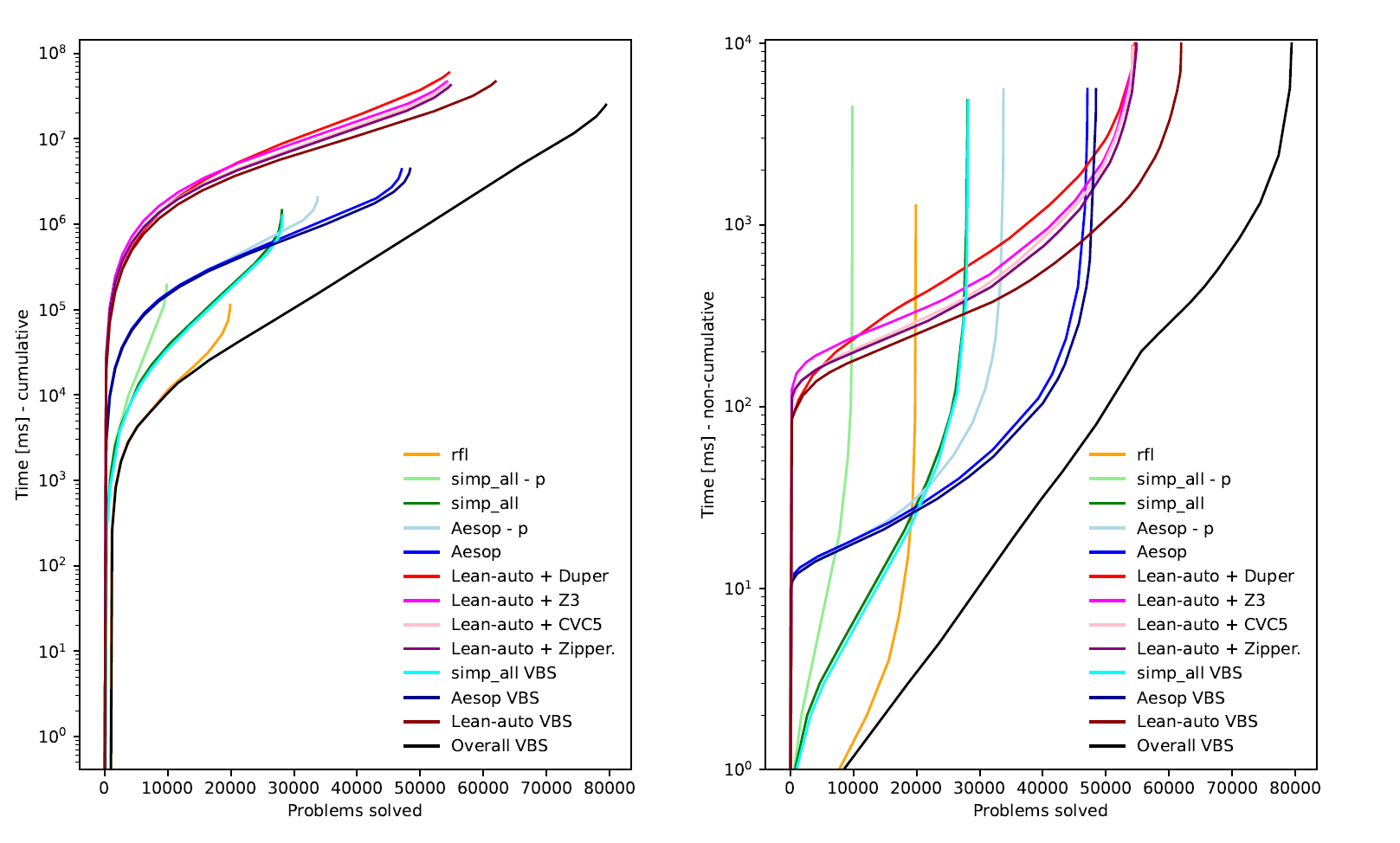
Figure 6: #Solved - Cumulative Time plot (left) and #Solved - Time plot (right)

Results are shown in Figure 5. For “simp_all”, “aesop,” and “Lean-auto,” we show the results of their virtual best solvers (VBSes). We compute unique solves among “rfl” and these three VBSes.

We find that Lean-auto solves more problems than all existing tools. Specifically, “Lean-auto + Duper”, which supports proof reconstruction, solves 36.6% problems in our benchmark set, which is 5.0% better than the best previous tool “Aesop”. The fact that “Lean-auto VBS” achieves 14.8% unique solves shows that Lean-auto is complementary to existing tools. The overall VBS, which combines Lean-auto and all existing tools, solves more than half (53.2%) of the problems in our benchmark set. On the other hand, Lean-auto is significantly slower than existing tools on solved problems. This is potentially caused by Lean-auto’s verified checker and the frequent definitional equality testing in Lean-auto’s monomorphization.

To better compare the performance of the various tools, we plot, for each tool, the number of solved problems vs. solving time and cumulative solving time. The results are shown in Figure 6. We see that Lean-auto is slower than existing tools on simple problems, but eventually solves more problems than all existing tools.

9 Conclusion

In this paper, we presented the ITP to ATP translation implemented in Lean-auto. Our contributions are three-fold. First, we addressed challenges posed by Lean 4’s dependent type theory and its various language features. Second, we designed a novel monomorphization procedure for dependent type theory. Finally, we implemented the translation procedure in Lean-auto and evaluated it on Mathlib4.

A possible direction for future work is to design a complete $\lambda_{\to}^{*}$ abstraction algorithm. Another direction is to investigate potential ways of handling existential type quantifiers and non-leading universal type quantifiers. We would also like to further investigate causes of Lean-auto’s inefficiencies and improve Lean-auto’s performance.

9.0.1 Acknowledgements

The authors thank: Prof. Jasmin Blanchette (Ludwig Maximilian University of Munich) for insightful discussions on the monomorphization procedure in Isabelle Sledgehammer; Mario Carneiro (Chalmers University of Technology) for helping us understanding implementation details of Lean 4; and Leonardo de Moura (Amazon Web Services) for his advice on the translation from Lean 4 to SMT solvers. We also greatly appreciate the help of the Lean Zulip users who answered our questions related to Lean 4 and Mathlib4. This work was supported in part by the Stanford Graduate Fellowship, the Stanford Center for Automated Reasoning, and AFRL and DARPA under Agreement FA8750-24-9-1000.

9.0.2

Clark Barrett is an Amazon Scholar.

Appendix 0.A Logical Symbols of $\lambda C$

$$\bot :=\forall p:\mathsf{U}_{0}.p\ \ \ (\neg):=\lambda p:\mathsf{U}_{0}.p\to\bot$$

$$(\land) :=\lambda p\ q:\mathsf{U}_{0}.\forall r:\mathsf{U}_{0}.(p\to q\to r)\to r$$

$$(\lor) :=\lambda p\ q:\mathsf{U}_{0}.\forall r:\mathsf{U}_{0}.(p\to r)\to(q\to r)\to r$$

$$(\leftrightarrow) :=\lambda p\ q.(p\to q)\land(q\to p)$$

$$(=_{\ell}) :=\lambda\alpha:\mathsf{U}_{\ell}.\lambda x\ y:\alpha.\forall p:\alpha\to\mathsf{U}_{0}.(p\ x\leftrightarrow p\ y)$$

$$(\exists_{\ell}) :=\lambda\alpha:\mathsf{U}_{\ell}.\lambda p:\alpha\to\mathsf{U}_{0}.\forall q:\mathsf{U}_{0}.((\forall x:\alpha.p\ x\to q)\to q)$$

Appendix 0.B Derivation Rules of PTS

The type judgement $\Gamma\vdash t:\alpha$ in a PTS specified by $(\mathcal{S},\mathcal{A},\mathcal{R})$ is defined by the following axioms and rules:

(axioms) $$\frac{}{\emptyset\vdash s_{1}:s_{2}} \text{if }(s_{1},s_{2})\in\mathcal{A}$$

(start) $$\frac{\Gamma\vdash A:s}{\Gamma,x:A\vdash x:A} \text{if }x\notin\Gamma$$

(weakening) $$\frac{\Gamma\vdash A:B\ \ \ \Gamma\vdash C:s}{\Gamma,x:C\vdash A:B} \text{if }x\notin\Gamma$$

(product) $$\frac{\Gamma\vdash A:s_{1}\ \ \ \Gamma,x:A\vdash B:s_{2}}{\Gamma\vdash(\forall x:A.B):s_{3}} \text{if }(s_{1},s_{2},s_{3})\in\mathcal{R}$$

(application) $$\frac{\Gamma\vdash f:(\forall x:A.B)\ \ \ \Gamma\vdash a:A}{\Gamma\vdash f\ a:B[x:=a]}$$

(abstraction) $$\frac{\Gamma,x:A\vdash b:B\ \ \ \Gamma\vdash(\forall x:A.B):s}{\Gamma\vdash(\lambda x:A.b):(\forall x:A.B)}$$

(conversion) $$\frac{\Gamma\vdash A:B\ \ \ \Gamma\vdash B^{\prime}:s\ \ \ B\cong B^{\prime}}{\Gamma\vdash A:B^{\prime}}$$

Appendix 0.C $\lambda C,\lambda_{\to}$ and $\lambda_{\to}^{*}$

Definition 2

$\lambda C$ is the pure type system $(\mathcal{S},\mathcal{A},\mathcal{R})$ where

$$\mathcal{S}:=\{\mathsf{U}_{\ell}|\ell\in\mathbb{N}\}\ \ \ \mathcal{A}:=\{(\mathsf{U}_{\ell},\mathsf{U}_{\ell+1})|\ell\in\mathbb{N}\}$$

$$\mathcal{R}:=\{(\mathsf{U}_{\ell},\mathsf{U}_{m},\mathsf{U}_{\mathsf{imax}(\ell,m)})|\ell\in\mathbb{N},m\in\mathbb{N}\}$$

$$\mathsf{imax}(m,n):=\left\{\begin{aligned} \mathsf{max}(m,n),&&n>0\\ 0,&&n=0\end{aligned}\right.$$

Definition 3

$\lambda_{\to}$ is the pure type system $(\mathcal{S},\mathcal{A},\mathcal{R})$ where

$$\mathcal{S}:=\{\mathsf{U}_{1},\mathsf{U}_{1}^{\prime}\}\ \ \ \mathcal{A}:=\{(\mathsf{U}_{1},\mathsf{U}_{1}^{\prime})\}\ \ \ \mathcal{R}:=\{(\mathsf{U}_{1},\mathsf{U}_{1},\mathsf{U}_{1})\}$$

This is equivalent to simply typed lambda calculus, where $\mathsf{U}_{1}$ and $\mathsf{U}_{1}^{\prime}$ are usually denoted as $*$ and $\square$, respectively.

Definition 4

$\lambda_{\to}^{*}$ is the pure type system $(\mathcal{S},\mathcal{A},\mathcal{R})$ where

$$\mathcal{S}:=\{\mathsf{U}_{\ell}|\ell\in\mathbb{N}^{*}\}\cup\{\mathsf{U}_{\ell}^{\prime}|\ell\in\mathbb{N}^{*}\}\ \ \ \mathcal{A}:=\{(\mathsf{U}_{\ell},\mathsf{U}_{\ell}^{\prime})|\ell\in\mathbb{N}^{*}\}$$

$$\mathcal{R}:=\{(\mathsf{U}_{\ell},\mathsf{U}_{m},\mathsf{U}_{\mathsf{max}\{l,m\}})|\ell\in\mathbb{N}^{*},m\in\mathbb{N}^{*}\}$$

Appendix 0.D HOL and $\text{HOL}^{*}$

Definition 5

HOL ($\text{HOL}^{*}$) is defined as $\lambda_{\to}$ ($\lambda_{\to}^{*}$) augmented with the following symbols:

1. $\mathsf{Bool}$

2. $\bot^{\prime}$ and $\to^{\prime}$

3. $\forall^{\prime}_{s}$, for each $s\in\mathcal{T}_{\to}^{*}$. Note that we are not requiring $s$ to be a type here because the typing rules below will ensure that $s$ must be a type in a well-formed $\forall_{s}^{\prime}$.

the following typing rules:

$$\frac{}{\vdash\mathsf{Bool}:\mathsf{U}_{1}}\ \ \ \ \frac{}{\Gamma\vdash\bot^{\prime}:\mathsf{Bool}}$$

$$\frac{}{\Gamma\vdash\to^{\prime}:\mathsf{Bool}\to\mathsf{Bool}\to\mathsf{Bool}}\ \ \ \ \frac{\Gamma\vdash s:\mathsf{U}_{\ell}}{\Gamma\vdash\forall^{\prime}_{s}:(s\to\mathsf{Bool})\to\mathsf{Bool}}$$

and the logical axioms and deduction rules of higher-order logic.

Note: The logical symbols $\neg^{\prime},\land^{\prime},\lor^{\prime},\leftrightarrow,=^{\prime}_{s},\exists^{\prime}_{s}$ are defined in a way consistent with their definition in $\lambda C$:

$$(\neg^{\prime}) :=\lambda(p:\mathsf{Bool}).(p\to^{\prime}\bot^{\prime})$$

$$(\land^{\prime}) :=\lambda(p\ q:\mathsf{Bool}).\forall(r:\mathsf{Bool}).((p\to^{\prime}q\to^{\prime}r)\to^{\prime}r)$$

$$(\lor^{\prime}) :=\lambda(p\ q:\mathsf{Bool}).\forall(r:\mathsf{Bool}).((p\to^{\prime}r)\to^{\prime}(q\to^{\prime}r)\to^{\prime}r)$$

$$(\leftrightarrow^{\prime}) :=\lambda(p\ q:\mathsf{Bool}).((p\to^{\prime}q)\land^{\prime}(q\to^{\prime}p))$$

$$(=^{\prime}_{s}) :=\lambda(x\ y:s).\forall(p:s\to\mathsf{Bool}).(p\ x\leftrightarrow^{\prime}p\ y)$$

$$(\exists^{\prime}_{s}) :=\lambda(p:s\to\mathsf{Bool}).\forall(q:\mathsf{Bool}).((\forall(x:s).p\ x\to^{\prime}q)\to^{\prime}q)$$

We use $\forall^{\prime}(x:s).t$ as a shorthand for $\forall^{\prime}_{s}\ (\lambda(x:s).t)$, and $\exists^{\prime}(x:\alpha).t$ as a shorthand for $\exists_{s}^{\prime}\ (\lambda(x:s).t)$.

For simplicity, the $\text{HOL}^{*}$ system we present in this paper only contains one symbol $\mathsf{Bool}$ for the type of propositions. In the implementation of Lean-auto, the $\text{HOL}^{*}$ system have a symbol $\mathsf{Bool}_{\ell}:\mathsf{U}_{\ell}$ for each universe level $\ell$, and each universe level have its own copy of logical symbols.

Appendix 0.E Universe Lifting

In this appendix, we discuss the translation procedure from $\text{HOL}^{*}$ to HOL in Lean-auto. For simplicity, universe lifting as presented in this section differs from Lean-auto’s implementation in terms of how $\mathsf{Bool}$ is handled.

First, we show that $\text{HOL}^{*}$ and HOL are, in a sense, equivalent to each other.

Definition 6

Let $\rho^{*}:\mathcal{T}_{\to}^{*}\to\mathcal{T}_{\to}$ be the mapping that forgets the universe levels, i.e.

$$\rho^{*}(\mathsf{Bool})=\mathsf{Bool}\ \ \ \ \ \ \rho^{*}(\mathsf{U}_{\ell})=\mathsf{U}_{1}\ \ \ \ \ \ \rho^{*}(\mathsf{U}_{\ell}^{\prime})=\mathsf{U}_{1}^{\prime}\ \ \ \ \ \ \rho^{*}(x)=x,\text{ for }x\in V$$

$$\rho^{*}(M\ N)=\rho^{*}(M)\ \rho^{*}(N)\ \ \ \ \ \ \rho^{*}(\lambda(x:s).M)=\lambda(x:\rho^{*}(s)).\rho^{*}(M)$$

$$\rho^{*}(\bot^{\prime})=\bot^{\prime}\ \ \ \ \ \ \rho^{*}(\to^{\prime})=\to^{\prime}\ \ \ \ \ \ \rho^{*}(\forall_{s}^{\prime})=\forall_{\rho^{*}(s)}^{\prime}$$

$\rho^{*}$ is extended to contexts as follows: $\rho^{*}(\emptyset):=\emptyset;\ \rho^{*}(\Gamma,x:\sigma):=\rho(\Gamma),x:\rho(\sigma)$

Definition 7

Let $\rho_{\ell}:\mathcal{T}_{\to}\to\mathcal{T}_{\to}^{*}(\ell\in\mathbb{N}^{*})$ be the mapping that turns $\mathsf{U}_{1}$ into $\mathsf{U}_{\ell}$, i.e.

$$\rho(\mathsf{Bool})=\mathsf{Bool}\ \ \ \ \ \ \rho(\mathsf{U}_{1})=\mathsf{U}_{\ell}\ \ \ \ \ \ \rho(\mathsf{U}_{1}^{\prime})=\mathsf{U}_{\ell}^{\prime}\ \ \ \ \ \ \rho(x)=x,\text{ for }x\in V$$

$$\rho(M\ N)=\rho(M)\ \rho(N)\ \ \ \ \ \ \rho(\lambda(x:s).M)=\lambda(x:\rho(s)).\rho(M)$$

$$\rho(\bot^{\prime})=\bot^{\prime}\ \ \ \ \ \ \rho(\to^{\prime})=\to^{\prime}\ \ \ \ \ \ \rho(\forall_{s}^{\prime})=\forall_{\rho(s)}^{\prime}$$

$\rho$ is extended to contexts as follows: $\rho(\emptyset):=\emptyset;\ \rho(\Gamma,x:\sigma):=\rho(\Gamma),x:\rho(\sigma)$

Theorem 0.E.1

For all $t\in\mathcal{T}_{\to}$, $\rho_{\ell}^{*}(\rho_{\ell}(t))=t$.

Proof

Induction on the construction rules of $\mathcal{T}_{\to}$.

Theorem 0.E.2

Forgetting universe levels preserves judgement, i.e., if $\Gamma\vdash t:s$ in $\text{HOL}^{*}$, then $\rho^{*}(\Gamma)\vdash\rho^{*}(t):\rho^{*}(s)$ in HOL.

Proof

Induction on the derivation rules of $\text{HOL}^{*}$.

Theorem 0.E.3

$\rho_{\ell}$ preserves judgement, i.e., if $\Gamma\vdash t:s$ in HOL, then $\rho_{\ell}(\Gamma)\vdash\rho_{\ell}(t):\rho_{\ell}(s)$ in $\text{HOL}^{*}$.

Proof

Induction on the derivation rules of HOL.

Theorem 0.E.4

$\text{HOL}^{*}$ and HOL are equivalent, i.e., if $\Gamma\vdash p:\mathsf{Bool}$ in $\text{HOL}^{*}$ and $p$ is provable in $\text{HOL}^{*}$, then $\rho^{*}(p)$ is provable in HOL; if $\Gamma\vdash p:\mathsf{Bool}$ in HOL and $p$ is provable in HOL, then $\rho_{\ell}(p)$ is provable in $\text{HOL}^{*}$ for any $\ell\in\mathbb{N}^{*}$.

Proof

Let $\mathcal{D}$ be a proof of $p$ in $\text{HOL}^{*}$, the a proof of $\rho^{*}(p)$ in HOL can be obtained by forgetting universe levels in $\mathcal{D}$. The converse can be proved in a similar way.

The universe lifting procedure in Lean-auto is the translation of $\text{HOL}^{*}$ to HOL in the context of $\lambda C$. In other words, it is the translation of the embedding of HOL in $\lambda C$ into an embedding of $\text{HOL}^{*}$ in $\lambda C$.

Definition 8

The $\ell$-embedding $\pi_{\ell}:\mathcal{T}_{\to}\to\mathcal{T}_{C}$ of HOL into $\lambda C$ is defined as $\pi_{\ell}:=\pi^{*}\circ\rho_{\ell}$, where $\pi^{*}$ is the canonical embedding of $\text{HOL}^{*}$ into $\lambda C$.

Definition 9

A universe lifting facility consists of three families of functions

1. $\mathsf{GLift}_{u,v}:\mathsf{U}_{u}\to\mathsf{U}_{\max\{u,v+1\}}$

2. $\mathsf{GLift.up}_{u,v}:\forall(\alpha:\mathsf{U}_{u}).\ \alpha\to\mathsf{GLift}_{u,v}\ \alpha$

3. $\mathsf{GLift.down}_{u,v}:\forall(\alpha:\mathsf{U}_{u}).\ \mathsf{GLift}_{u,v}\ \alpha\to\alpha$

where $u,v\in\mathbb{N}$, such that they satisfy the following bijectivity condition:

$$\forall(\alpha:\mathsf{U}_{u}).\mathsf{GLift.up}_{u,v}\ \alpha\circ\mathsf{GLift.down}_{u,v}\ \alpha=\lambda(x:\mathsf{GLift}_{u,v}\ \alpha).x$$

$$\forall(\alpha:\mathsf{U}_{u}).\mathsf{GLift.down}_{u,v}\ \alpha\circ\mathsf{GLift.up}_{u,v}\ \alpha=\lambda(x:\alpha).x$$

In Lean 4, universe lifting facility can be realized by the following inductive type:

⬇

structure GLift.{u, v} (α : Sort u) : Sort (max u (v + 1)) where

/– Lift a value into ‘GLift α‘ -/ up ::

/– Extract a value from ‘GLift α‘ -/ down : α

Theorem 0.E.5

Assume the existence of a universe lifting facility in $\lambda C$. Then, for all $\ell\in\mathbb{N}$, there exists two families of $\lambda C$ functions

$$\mathsf{Up}_{s}:s\to\mathsf{UpType}\ s\ \ \ \mathsf{Down}_{s}:\mathsf{UpType}\ s\to s$$

for sorts $s:\mathsf{U}_{\ell^{\prime}},\ell^{\prime}\leq\ell+1$, satisfying the bijectivity conditions

$$\mathsf{Up}_{s}\circ\mathsf{Down}_{s}=\lambda(x:\mathsf{UpType}\ s).x\ \ \ \mathsf{Down}_{s}\circ\mathsf{Up}_{s}=\lambda(x:s).s$$

and the congruence condition

$$\forall(f:\alpha\to\beta).\ \mathsf{Up}_{\beta}\ (f\ x)=(\mathsf{Up}_{\alpha\to\beta}\ f)\ (\mathsf{Up}_{\alpha}\ x)$$

where $\mathsf{UpType}$ is recursively defined as follows:

$$\mathsf{UpType}\ x =\mathsf{GLift}_{\ell^{\prime},\ell}\ x,\text{ for }x\in V$$

$$\mathsf{UpType}\ (\alpha\to\beta) =\mathsf{UpType}\ \alpha\to\mathsf{UpType}\ \beta$$

Proof

Structural induction on $s$

1. If $s=a$, where $a\in V$ is a variable, then we can define

   $$\mathsf{Up}_{a}:=\mathsf{GLift.up}_{\ell^{\prime},\ell}\ a\ \ \ \mathsf{Down}_{a}:=\mathsf{Glift.down}_{\ell^{\prime},\ell}\ a$$

2. If $s=(\alpha\to\beta)$ and the induction hypothesis holds for $\alpha$ and $\beta$, then we can define

   $$\mathsf{Up}_{\alpha\to\beta} =\lambda(f:\alpha\to\beta)\ (x:\mathsf{UpType}\ \alpha).\ \mathsf{Up}_{\beta}\ (f\ (\mathsf{Down}_{\alpha}\ x))$$

   $$\mathsf{Down}_{\alpha\to\beta} =\lambda(f:\mathsf{UpType}\ \alpha\to\mathsf{UpType}\ \beta)\ (x:\alpha).\ \mathsf{Down}_{\beta}\ (f\ (\mathsf{Up}_{\alpha}\ x))$$

The rationale of $\mathsf{UpType}\ (\alpha\to\beta):=\mathsf{UpType}\ \alpha\to\mathsf{UpType}\ \beta$ is that, given $f\ x$ in the canonical embedding of $\text{HOL}^{*}$, where $f:\alpha\to\beta$ and $x:\alpha$, we would like $(\mathsf{Up}_{\alpha\to\beta}\ f)\ (\mathsf{Up}_{\alpha}\ x)$ to be type correct.

Given $\mathsf{Up}_{s}$, $\mathsf{Down}_{s}$ and $\mathsf{UpType}$ satisfying Theorem 0.E.5 with $\ell$ taken to be larger than all universe levels in the input terms, the universe lifting procedure, or the translation of the canonical embedding of $\text{HOL}^{*}$ into the $\ell$-embedding of HOL, denoted as $\mathsf{ULiftTrans}$, works as follows:

1. If $x$ is a variable and $x:s$, then $\mathsf{ULiftTrans}(x):=x^{\prime}$. If $x$ is not a free variable, then we define $x^{\prime}$ as $x^{\prime}:=\mathsf{Up}_{s}\ x$ in Lean 4. If $x$ is a bound variable, no further operation is needed.

2. $\mathsf{ULiftTrans}(f\ x):=\mathsf{ULiftTrans}(f)\ \mathsf{ULiftTrans}(x)$

3. $\mathsf{ULiftTrans}(\lambda(x:s).\ y):=\lambda(x^{\prime}:\mathsf{UpType}\ s).\ \mathsf{ULiftTrans}(y)$

It’s easy to verify that $\mathsf{ULiftTrans}(e)$ is definitionally equal to $\mathsf{Up}_{s}\ e$ for all terms $e:s$ in the canonical embedding of $\text{HOL}^{*}$.

Appendix 0.F Essentially Higher-order Problem

In this appendix, we give a formal definition of essentially higher-order problems (EHOPs) and discuss some of its theoretical properties.

Definition 10

Let $\sigma:V\to\mathcal{T}_{C}$ be a mapping. Define its extension $\overline{\sigma}:\mathcal{T}_{C}\to\mathcal{T}_{C}$ as

$$\overline{\sigma}(\mathsf{U}_{\ell}):=\mathsf{U}_{\ell}\ \ \ \ \ \ \overline{\sigma}(x):=\sigma(x),\text{ for }x\in V\ \ \ \ \ \ \overline{\sigma}(M\ N):=\overline{\sigma}(M)\ \overline{\sigma}(M)$$

$$\overline{\sigma}(\lambda x:s.M):=\lambda x:\overline{\sigma}(s).\overline{\sigma[x\mapsto x]}(M)$$

$$\overline{\sigma}(\forall x:s.M):=\forall x:\overline{\sigma}(s).\overline{\sigma[x\mapsto x]}(M)$$

where

$$\sigma[u\to t](x):=\left\{\begin{aligned} &t&&x=u\\ &\sigma(x)&&x\in V\backslash\{u\}\end{aligned}\right.$$

Definition 11

A substitution is a triple $(\Gamma,\Gamma^{\prime},\sigma)$ where $\Gamma,\Gamma^{\prime}$ are $\lambda C$ contexts and $\sigma:V\to\mathcal{T}_{C}$, such that for all $(u:\tau)\in\Gamma$,

$$\Gamma^{\prime}\vdash\sigma(u):\overline{\sigma}(\tau)$$

$\Gamma$ is called the domain of the substitution, and $\Gamma^{\prime}$ is called the codomain of the substitution.

Theorem 0.F.1

Let $(\Gamma,\Gamma^{\prime},\sigma)$ be a substitution. If $\Gamma\vdash t:s$, then $\Gamma^{\prime}\vdash\overline{\sigma}(t):\overline{\sigma}(s)$

Proof

Induction on the derivation of $\Gamma\vdash t:s$.

Definition 12

Let $\Gamma$ be a $\lambda C$ context and $t_{1},t_{2}$ be $\lambda C$ terms. If variable set $M$ and substitution $(\Gamma,\Gamma^{\prime},\sigma)$ satisfies

1. There exists a $\lambda C$ term $s$ such that $\Gamma^{\prime}\vdash\overline{\sigma}(t_{1}):s$ and $\Gamma^{\prime}\vdash\overline{\sigma}(t_{2}):s$.

2. $\overline{\sigma}(t_{1})\cong\overline{\sigma}(t_{2})$ (i.e., $\overline{\sigma}(t_{1})$ and $\overline{\sigma}(t_{2})$ are $\beta\eta$-equivalent)

3. For all variables $v\in\Gamma\backslash M$, $\sigma(v)=v$.

Then $(\Gamma,\Gamma^{\prime},\sigma)$ is called a $M$-unifier of $t_{1}$ and $t_{2}$. In the context of Lean, this corresponds to a unifier of $t_{1}$ and $t_{2}$ under context $\Gamma$, with $M$ as the set of metavariables.

Definition 13

The canonical embedding $\pi^{*}:\mathcal{T}_{\to}^{*}\to\mathcal{T}_{C}$ of $\text{HOL}^{*}$ into $\lambda C$ is defined as follows:

$$\pi^{*}(\mathsf{Bool})=\mathsf{U}_{0}\ \ \ \ \ \ \pi^{*}(\mathsf{U}_{\ell})=\mathsf{U}_{\ell}\ \ \ \ \ \ \pi^{*}(\mathsf{U}_{\ell}^{\prime})=\mathsf{U}_{\ell+1}\ \ \ \ \ \ \pi^{*}(x)=x,\text{ for }x\in V$$

$$\pi^{*}(M\ N)=\pi^{*}(M)\ \pi^{*}(N)\ \ \ \ \ \ \pi^{*}(\lambda(x:s).M)=\lambda(x:\pi^{*}(s)).\pi^{*}(M)$$

$$\pi^{*}(\bot^{\prime})=\forall(\alpha:\mathsf{U}_{0}).\alpha\ \ \ \ \ \ \ \ \ \ \pi^{*}(\to^{\prime})=\lambda(p\ q:\mathsf{U}_{0}).p\to q$$

$$\pi^{*}(\forall_{s}^{\prime})=\lambda(p:\pi^{*}(s)\to\mathsf{U}_{0}).\forall(x:\pi^{*}(s)).p\ x$$

$\pi^{*}$ is extended to contexts as follows: $\pi^{*}(\emptyset):=\emptyset,\pi^{*}(\Gamma,x:\sigma):=\pi^{*}(\Gamma),x:\pi^{*}(\sigma)$

Theorem 0.F.2

Canonical embedding preserves judgement, i.e. if $\Gamma\vdash t:s$ in $\text{HOL}^{*}$, then $\pi^{*}(\Gamma)\vdash\pi^{*}(t):\pi^{*}(s)$ in $\lambda C$

Proof

Induction on the derivation rules of $\text{HOL}^{*}$.

Definition 14

An ($\text{HOL}^{*}/\lambda C$) problem is a tuple $(\Gamma,p)$, denoted as $\Gamma\vdash?p$, where $\Gamma$ is a ($\text{HOL}^{*}/\lambda C$) context, called the hypotheses of the problem, and $p$ is an ($\text{HOL}^{*}/\lambda C$) term, called the goal of the problem. A $\lambda C$ problem $\Gamma\vdash?p$ is provable iff there exists a $\lambda C$ term $t$ such that $\Gamma\vdash t:p$. An $\text{HOL}^{*}$ problem $\Gamma\vdash?p$ is provable iff there exists a $\lambda C$ term $t$ such that $\pi^{*}(\Gamma)\vdash t:\pi^{*}(p)$.

Definition 15

A $\lambda C$ problem $\Gamma\vdash?p$ is essentially higher-order provable (EHOP) iff there exists a provable $\text{HOL}^{*}$ problem $\Gamma^{\prime}\vdash?p^{\prime}$ and a substitution $(\pi^{*}(\Gamma^{\prime}),\allowbreak\Gamma,\sigma)$ such that $p\cong\overline{\sigma}(\pi^{*}(p^{\prime}))$.

Theorem 0.F.3

If a $\lambda C$ problem $\Gamma\vdash?p$ is EHOP, then it is provable.

Proof

By the definition of EHOP, there exists a provable $\text{HOL}^{*}$ problem $\Gamma^{\prime}\vdash?p^{\prime}$ and substitution $(\pi^{*}(\Gamma^{\prime}),\Gamma,\sigma)$ such that $p\cong\overline{\sigma}(\pi^{*}(p^{\prime}))$. By the definition of $\text{HOL}^{*}$ provability, there exists a term $t^{\prime}$ such that $\pi^{*}(\Gamma^{\prime})\vdash t^{\prime}:\pi^{*}(p^{\prime})$. By Theorem 0.F.2, $\Gamma\vdash\overline{\sigma}(t^{\prime}):\overline{\sigma}(\pi^{*}(p^{\prime}))$, thus $\Gamma\vdash?p$ is provable.

We assume that excluded middle is implicitly contained in the hypotheses of all $\text{HOL}^{*}$ and $\lambda C$ problems. In $\lambda C$, excluded middle is $\mathsf{em}:\forall(p:\mathsf{U}_{0}),p\lor\neg p$; in $\text{HOL}^{*}$, it is $\mathsf{em}^{\prime}:\forall(p:\mathsf{Bool}).p\lor^{\prime}\neg^{\prime}p$.

Example 1

Consider the $\lambda C$ problem $\Gamma\vdash?p$ where

$$\Gamma:=\ \mathbb{N}:\mathsf{U}_{1},\mathsf{Fin}:\mathbb{N}\to\mathsf{U}_{1},\mathsf{add}:\forall(n:\mathbb{N}).(\mathsf{Fin}\ n\to\mathsf{Fin}\ n\to\mathsf{Fin}\ n),n:\mathbb{N}$$

$$p:=\ (\forall(u\ v:\mathsf{Fin}\ n).\mathsf{add}\ n\ u\ v=_{1}\mathsf{add}\ n\ v\ u)\to$$

$$\ \ \ \forall(u\ v\ w:\mathsf{Fin}\ n).\mathsf{add}\ n\ (\mathsf{add}\ n\ x\ y)\ z=_{1}\mathsf{add}\ n\ z\ (\mathsf{add}\ n\ y\ x)$$

Given

$$\Gamma^{\prime}:=\ \alpha:\mathsf{U}_{1},f:\alpha\to\alpha\to\alpha$$

$$p^{\prime}:=\ (\forall^{\prime}(u\ v:\alpha).f\ u\ v=_{\alpha}^{\prime}f\ v\ u)\to^{\prime}$$

$$\ \ \ \forall^{\prime}(u\ v\ w:\alpha).f\ (f\ u\ v)\ w=_{\alpha}^{\prime}f\ w\ (f\ v\ u)$$

The $\text{HOL}^{*}$ problem $\Gamma^{\prime}\vdash?p^{\prime}$ is provable. Moreover, given

$$\sigma(\alpha):=\mathsf{Fin}\ n,\sigma(f):=\mathsf{add}\ n$$

The triple $(\pi^{*}(\Gamma^{\prime}),\Gamma,\sigma)$ forms a substitution, and $p\cong\overline{\sigma}(\pi^{*}(p^{\prime}))$. Therefore, $\Gamma\vdash?p$ is EHOP.

Note that moving implications in the goal into hypotheses (and vice versa) may change the EHOP status of a problem. For example,

$$\alpha:\mathsf{U}_{1},x:\alpha,p:\alpha\to\mathsf{U}_{0}\ \vdash?\ (p\ x\to p\ x)$$

is EHOP. However, if we introduce $p\ x$ into the hypotheses, the problem is no longer EHOP:

$$\alpha:\mathsf{U}_{1},x:\alpha,p:\alpha\to\mathsf{U}_{0},h:p\ x\ \vdash?\ p\ x$$ (2)

Theorem 0.F.4

The $\lambda C$ problem (2) is provable but not EHOP.

Proof

Note that $h:p\ x$ under the hypotheses of (2), thus (2) is provable. To show that (2) is not EHOP, we use proof by contradiction. Suppose there is an $\text{HOL}^{*}$ problem $\Gamma^{\prime}\vdash?p^{\prime}$ and a substitution $(\Gamma^{\prime},\Gamma,\sigma)$ such that $p\ x\cong\overline{\sigma}(\pi^{*}(p^{\prime}))$. Then, the $\beta\eta$ normal form of $p^{\prime}$ must be of the form $f\ t_{1}\ \dots\ t_{k}$ where $f$ is a free variable. Note that $\Gamma^{\prime}$, as a context of $\lambda_{\to}^{*}$, consists solely of $\text{HOL}^{*}$ (type or term) variable declarations, and cannot contain premises like $\lambda C$ contexts. Note that there exists models where $f\ t_{1}\ \dots\ t_{k}$ is false, for example when $f$ is a function that takes $k$ arguments and always returns $\bot$. Therefore, $\Gamma^{\prime}\vdash?p^{\prime}$ is not provable in $\text{HOL}^{*}$, thus $(2)$ is not EHOP.

Appendix 0.G $\lambda_{\to}^{*}$ Abstraction Algorithm

In this appendix, we give a formal presentation of the $\lambda_{\to}^{*}$ abstraction algorithm. When given a $\lambda C$ problem $\Gamma\vdash?p$, the algorithm attempts to find a $\lambda_{\to}^{*}$ problem $\Gamma^{\prime}\vdash?p^{\prime}$ and a substitution $(\pi^{*}(\Gamma^{\prime}),\Gamma,\sigma)$ such that $p\cong\overline{\sigma}(\pi^{*}(p^{\prime}))$, and that $p^{\prime}$ retains as much information in $p$ as possible.

Note that the output of Lean-auto’s quantifier instantiation is a list of $\lambda C$ terms $h_{1},\dots,h_{n}$, and we would like to prove $\bot$ using these terms. Suppose the $\lambda C$ context of the problem is $\Gamma$. According to the above discussion, the input to the $\lambda_{\to}^{*}$ abstraction algorithm should be $\Gamma\vdash?\ (h_{1}\to\dots\to h_{n}\to\bot)$. In practice, we run $\lambda_{\to}^{*}$ abstraction consecutively on each of $h_{i}(1\leq i\leq n)$ under context $\Gamma$, which produces equivalent results. Therefore, we can either think of the input of $\lambda_{\to}^{*}$ abstraction as one $\lambda C$ term $h_{1}\to\dots\to h_{n}\to\bot$, or as a list of $\lambda C$ terms $h_{1},\dots,h_{n}$.

First, we give a formal definition of dependent arguments. This definition accounts for the fact that dependent arguments are dynamic. Note that in the argument list of functions, dependent and non-dependent arguments may interleave with each other.

Definition 16

Suppose $\Gamma\vdash s:\mathsf{U}_{l}$ in $\lambda C$. If $s=(\forall(x:s_{1}).s_{2})$ and $x$ occurs in $s_{2}$, then $s$ is said to be a $\Gamma$-leading argument dependent type, denoted as $\mathsf{LADT}(\Gamma;s)$. Suppose $\Gamma\vdash t:s$ in $\lambda C$, where $s$ is in $\beta$ normal form. If $\mathsf{LADT}(\Gamma;s)$, then $t$ is said to be $\Gamma$-leading argument dependent ($\Gamma$-lad), denoted as $\mathsf{LAD}(\Gamma;t)$.

Definition 17

Suppose the term $a_{0}\ a_{1}\ \dots\ a_{k}$ is type correct under context $\Gamma$ in $\lambda C$. Then for $1\leq i\leq k$, $a_{0}$ is said to have dependent $i$-th argument with respect to $\Gamma$ and argument list $(a_{1},\dots,a_{k})$, or $i$-dep w.r.t $\Gamma$ and $(a_{1},\dots,a_{k})$, iff $\mathsf{LAD}(\Gamma;a_{0}\ a_{1}\ \dots\ a_{i-1})$. For convenience, we use the predicate

$$\mathsf{Dep}(\Gamma;a_{0},(a_{1},\dots,a_{k}),i)\ \ \ (k\geq 0,1\leq i\leq k)$$

to denote that $a_{0}$ is $i$-dep w.r.t $\Gamma$ and $(a_{1},\dots,a_{k})$. Furthermore, we define

$$\mathsf{LFun}(\Gamma;a_{0},(a_{1},\dots,a_{k})):=\lambda(x_{i_{1}}:s_{i_{1}})\dots(x_{i_{m}}:s_{i_{m}}).a_{0}\ w_{1}\ \dots\ w_{m}$$

$$\mathsf{DArgs}(\Gamma;a_{0},(a_{1},\dots,a_{k})):=(b_{i_{1}},\dots,b_{i_{m}})$$

$$\mathsf{LArgs}(\Gamma;a_{0},(a_{1},\dots,a_{k})):=(a_{j_{1}},\dots,a_{j_{k-m}})$$

where $i_{1}<i_{2}<\dots<i_{m}$ are all the arguments that are dependent, $j_{1}<j_{2}<\dots<j_{k-m}$ are all the arguments that are non-dependent, $\Gamma\vdash a_{i}:s_{i}$, and

$$w_{i}:=\left\{\begin{aligned} a_{i},&&\mathsf{Dep}(\Gamma;a_{0},(a_{1},\dots,a_{k}),i)\\ x_{i},&&\text{otherwise}\end{aligned}\right.$$

Example 2

Let

$$\Gamma:= \ \mathsf{compose}:\forall(\beta\ \gamma:\mathsf{U}_{1}).(\beta\to\gamma)\to\forall(\alpha:\mathsf{U}_{1}).(\alpha\to\beta)\to(\alpha\to\gamma),$$

$$\ A:\mathsf{U}_{1},B:\mathsf{U}_{1},C:\mathsf{U}_{1},f:B\to C,g:A\to B,x:A$$

Then

$$\mathsf{compose},\mathsf{compose}\ B,\mathsf{compose}\ B\ C\ f$$

are $\Gamma$-lad, while

$$\mathsf{compose}\ B\ C,\mathsf{compose}\ B\ C\ f\ A,\mathsf{compose}\ B\ C\ f\ A\ g$$

are not. Therefore, the dependent arguments of $\mathsf{compose}$ w.r.t $(B,C,f,A,g,x)$ are $1,2$ and $4$, and we have

$$\mathsf{LFun}(\Gamma;\mathsf{compose},(A,B,C,f,g,x))=\lambda(f:B\to C).\mathsf{compose}\ A\ B\ f\ C$$

$$\mathsf{LArgs}(\Gamma;\mathsf{compose},(A,B,C,f,g,x))=(f,g,x)$$

Example 3

Let

$$\Gamma:=\mathsf{func}:\forall(\alpha:\mathsf{U}_{1}\to\mathsf{U}_{1})\ (\beta:\mathsf{U}_{1}).\alpha\ \beta,A:\mathsf{U}_{1},B:\mathsf{U}_{1}$$

Then $\mathsf{func}$ is $\Gamma$-lad, while

$$\mathsf{func}\ (\lambda\beta.A):\mathsf{U}_{1}\to A\ \ \ \ \ \ \mathsf{func}\ (\lambda\beta.A)\ B:A$$

are not. Therefore, the dependent argument of $\mathsf{func}$ w.r.t $(\lambda\beta.A,B)$ is $1$, and we have

$$\mathsf{LFun}(\Gamma;\mathsf{func},(\lambda\beta.A,B))=\mathsf{func}\ (\lambda\beta.A)\ \ \ \ \ \ \mathsf{LArgs}(\Gamma;\mathsf{func},(\lambda\beta.A,B))=B$$

Now, we define quasi-monomorphic terms, the set of $\lambda C$ terms that $\lambda_{\to}^{*}$ abstraction can successfully translate to $\text{HOL}^{*}$. The predicate $\mathsf{QMono}(\Gamma;B,t)$ will be used to represent “$t$ is a quasi-monomorphic term under context $\Gamma$, with variables in $B$ being bound variables”. It is used both in $\lambda_{\to}^{*}$ abstraction and in quantifier instantiation.

Definition 18

We define the predicate $\mathsf{QMono}(\Gamma;B,t)$ inductively, where $\Gamma$ is a $\lambda C$ context, $B$ is a set of variables, and $t$ is a $\lambda C$ term

1. For variable $x\in B$ and terms $t_{1},\dots,t_{n}$,

   $$\mathsf{QMono}(\Gamma;B,x\ t_{1}\dots\ t_{n}):=\ \mathsf{DArgs}(\Gamma;x,(t_{1}\ \dots\ t_{n}))=\emptyset\land$$

   $$\forall i\in\{1,\dots,n\}.\mathsf{QMono}(\Gamma;B,t_{i})$$

2. For variable $x\notin B$ and terms $t_{1},\dots,t_{n}$,

   $$\mathsf{QMono}(\Gamma;B,x\ t_{1}\dots\ t_{n}):=\ (\forall t\in\mathsf{DArgs}(\Gamma;x,(t_{1},\dots,t_{n})).FV(t)\cap B=\emptyset)\land$$

   $$(\forall t\in\mathsf{LArgs}(\Gamma;x,(t_{1},\dots,t_{n})).\mathsf{QMono}(\Gamma;B,t))$$

3. For variable $x$ and terms $s,t$

   $$\mathsf{QMono}(\Gamma;B,\lambda(x:s).t):=\ FV(s)\cap B=\emptyset\land(\Gamma\not\vdash s:\mathsf{U}_{0})$$

   $$\land\mathsf{QMono}(\Gamma,x:s;B\cup\{x\},t)$$

4. For variable $x$ and terms $s,t$ such that $x\in FV(t)$,

   $$\mathsf{QMono}(\Gamma;B,\forall(x:s).t):=\ \neg FV(s)\cap B=\emptyset\land(\Gamma\not\vdash s:\mathsf{U}_{0})\land(\Gamma\vdash t:\mathsf{U}_{0})\land$$

   $$\mathsf{QMono}(\Gamma,x:s;B\cup\{x\},t)$$

5. For terms $s,t$,

   $$\mathsf{QMono}(\Gamma;B,s\to t):=\ (\Gamma\vdash s:\mathsf{U}_{0})\land(\Gamma\vdash t:\mathsf{U}_{0})\land$$

   $$\mathsf{QMono}(\Gamma;B,s)\land\mathsf{QMono}(\Gamma;B,t)$$

According to the definition of $\mathsf{QMono}$, terms coming from canonical embedding of $\text{HOL}^{*}$ terms are automatically quasi-monomorphic, e.g.

$$\mathsf{QMono}(\alpha:\mathsf{U}_{1},p:(\alpha\to\alpha)\to\mathsf{U}_{0};\emptyset,\forall(p:\alpha\to\alpha).f\ p)$$

Proofs are not allowed to be quantified by $\lambda$ or dependent $\forall$ binders:

$$\neg\mathsf{QMono}(p:\mathsf{U}_{0},q:p\to\mathsf{U}_{0};\emptyset,\forall(x:p).q\ x)$$

Occurrence of a dependently typed free variable does not break the quasi-monomorphic property iff its dependent arguments do not contain bound variables (assuming $B=\emptyset$):

$$\mathsf{QMono}( \mathbb{N}:\mathsf{U}_{1},\mathsf{Fin}:\mathbb{N}\to\mathsf{U}_{1},\mathsf{add}:\forall(n:\mathbb{N}).\mathsf{Fin}\ n\to\mathsf{Fin}\ n\to\mathsf{Fin}\ n,k:\mathbb{N};$$

$$\emptyset,\forall(x\ y:\mathsf{Fin}\ k).\mathsf{add}\ k\ x\ y=\mathsf{add}\ k\ y\ x)$$

Occurrence of a dependently typed bound variable does not break the quasi-monomorphic property iff its dependent arguments are not instantiated:

$$\mathsf{QMono}(\emptyset;\emptyset,\lambda(f:(\forall(\alpha:\mathsf{U}_{0}).\alpha)\to(\forall(\alpha:\mathsf{U}_{0}).\alpha))\ (x:\forall(\alpha:\mathsf{U}_{0}).\alpha).f\ x)$$

Except for within type declarations of bound variables, bodies of $\forall$ abstractions must be propositions:

$$\neg\mathsf{QMono}(\alpha:\mathsf{U}_{1},\beta:\alpha\to\mathsf{U}_{1};\emptyset,\forall(x:\alpha).\beta\ x)$$

Function lamAbst($\Gamma;B,t$)

    In : $\lambda C$ context $\Gamma$, variable set $B$, and $\lambda C$ term $t$ satisfying $\mathsf{QMono}(\Gamma;B,t)$

    Out : a $\lambda_{\to}^{*}$ term

    match t  with

       case $a\ b$  /* Function application */

          $f:=\mathsf{getAppFn}(t)$

          $\mathit{args}:=\mathsf{getAppArgs}(t)$

          if $f\in B$ then

             for $a:\mathit{args}$ do

               $a:=\mathsf{lamAbst}(\Gamma;B,a)$

            

            return $\mathsf{mkAppN}(f,\mathit{args})$

          $\mathit{lf}:=\mathsf{LFun}(\Gamma;f,\mathit{args})$

          $\mathit{largs}:=\mathsf{LArgs}(\Gamma;f,\mathit{args})$

          $\mathit{lvar}:=\mathsf{getLVarName}(\mathit{lf})$

          return $\mathsf{mkAppN}(\mathit{lvar},\mathit{largs})$

      

      case $\forall(v:a).b$ 

          $\mathit{atype}:=\mathsf{inferType}(\Gamma;a)$

          $\mathit{babst}:=\mathsf{lamAbst}(\Gamma,v:a;B\cup\{v\},b)$

          if $\mathit{atype}=\mathsf{U}_{0}$ then

             $\mathit{aabst}:=\mathsf{lamAbst}(\Gamma;B,a)$

             return $\mathit{aabst}\to\mathit{babst}$

          return $\forall(v:a).\mathit{babst}$

      

      case $\lambda(v:a).b$ 

          $\mathit{babst}:=\mathsf{lamAbst}(\Gamma,v:a;B\cup\{v\},b)$

          return $\lambda(v:a).\mathit{babst}$

      

      otherwise

         return $\mathsf{getLVarName}(t)$

      

      

   

   

end

Function getLVarName(t)

    In : $\lambda C$ term $t$

    Out : $\lambda_{\to}^{*}$ variable name corresponding to $t$

    if $H.\mathsf{contains}(t)$ then

       return $H.\mathsf{find}(t)$

    $\mathit{newname}:=\mathsf{freshVarName}()$

    $H.\mathsf{add}(t,\mathit{newname})$

    return $\mathit{newname}$

end

Algorithm 2 $\lambda_{\to}^{*}$ abstraction algorithm of Lean-auto

Now, we describe the $\lambda_{\to}^{*}$ abstraction procedure $\mathsf{lamAbst}$ of Lean-auto. The algorithm is shown in Algorithm 2. A global hash map $H$ is used to record the $\text{HOL}^{*}$ variables associated with abstracted $\lambda C$ terms. A few auxiliary functions are used in the algorithm:

1. For a term $t$, if $t$ is in $H$, then $\mathsf{getLVarName}(t)$ returns the $\text{HOL}^{*}$ free variable corresponding to $t$, otherwise it creates a new $\text{HOL}^{*}$ free variable for $t$.

2. For a term $t=w\ t_{1}\ \dots\ t_{n}$ where $w$ is not an application, $\mathsf{getAppFn}(t)=w,\mathsf{getAppArgs}(t)=(t_{1},\dots,t_{n})$.

3. For terms $w,t_{1},\dots,t_{n}$, $\mathsf{mkAppN}(w,(t_{1},\dots,t_{n}))=w\ t_{1}\ \dots\ t_{n}$.

4. For a context $\Gamma$ and a term $t$, $\mathsf{inferType}(\Gamma,t)$ computes the $\beta$-normal form of the type of $t$ under $\Gamma$.

Note that $\mathsf{lamAbst}$ only returns the $\text{HOL}^{*}$ problem (as a $\text{HOL}^{*}$ term). The “substitution” from $\text{HOL}^{*}$ to $\lambda C$ needs to be obtained by computing the inverse of $H$ after the execution of the algorithm. Also, note that the implementation of this algorithm in Lean-auto checks whether $t$ breaks the requirements of quasi-monomorphic-ness and fails if it does. For simplicity, these checks have been omitted in $\mathsf{lamAbst}$.

Appendix 0.H Quantifier Instantiation

In this appendix, we present the technical details of Lean-auto’s quantifier instantiation procedure. First, we give a formal definition of instance:

Definition 19

Let $\Gamma$ be a $\lambda C$ context, and $t$ be a $\lambda C$ term which is type correct under $\Gamma$.

1. A constant instance of $t$ is a $\lambda C$ term of the form $\lambda(x_{1}:s_{1})\dots(x_{m}:s_{m}).t\ t_{1}\ \dots\ t_{k}$ that is type correct under $\Gamma$, where $s_{1},\dots,s_{m},t_{1},\dots t_{k}$ are $\lambda C$ terms.

2. For $t=\forall(x_{1}:r_{1})\dots(x_{n}:r_{n}).b$, a hypothesis instance of $t$ is a $\lambda C$ term of the form $\forall(y_{1}:s_{1})\dots(y_{m}:s_{m}).b[t_{1}/x_{1}]\dots[t_{n}/x_{n}]$, where $s_{1},\dots,s_{m},t_{1},\dots,t_{n}$ are $\lambda C$ terms, and $t_{1}[t_{2}/x]$ stands for the term obtained by replacing all the $x$ in $t_{1}$ with $t_{2}$.

Unless otherwise stated, when discussing instances of functions, we will always be referring to constant instances; when discussing instances of hypotheses, we will always be referring to hypothesis instances. An instance of a function is called an $\text{HOL}^{*}$ instance iff all of the function’s dependent arguments are instantiated with terms that do not contain bound variables. Formally, the set of all $\text{HOL}^{*}$ instances in a $\lambda C$ term is defined as follows:

Definition 20

Let $\Gamma$ be a $\lambda C$ context and $B$ be a set of variables, then

1. For variable $x$ and terms $t_{1},\dots,t_{n}$,

   $$\mathsf{holInsts}(\Gamma;B,x\ t_{1}\ \dots\ t_{n}):=\left\{\begin{aligned} S\cup\{l\},&&FV(l)\cap B=\emptyset\\ S,&&\text{otherwise}\end{aligned}\right.$$

   where

   $$l:=\mathsf{LFun}(\Gamma;x,(t_{1}\ \dots\ t_{n}))\ \ \ \ \ \ S:=\bigcup_{t\in\mathsf{LArgs}(\Gamma;x,(t_{1},\dots,t_{n}))}\mathsf{holInsts}(\Gamma;V,t)$$

2. For variable $x$ and terms $a,b$,

   $$\mathsf{holInsts}(\Gamma;B,\forall(x:a).b)=\mathsf{holInsts}(\Gamma;B,\lambda(x:a).b)$$

   $$:=\mathsf{holInsts}(\Gamma;B,a)\cup\mathsf{holInsts}(\Gamma,x:a;B\cup\{x\},b)$$

3. Otherwise, $\mathsf{holInsts}(\Gamma;B,t):=\emptyset$.

Function match($\Gamma;M,m,h$)

    In : $\lambda C$ context $\Gamma$, variable set $M$, and $\lambda C$ terms $m,h$

    Out : A set of unifiers

    match h  with

       case $a\ b$  /* Function application */

          $\mathit{matches}:=\emptyset$

          $f:=\mathsf{getAppFn}(t)$

          $\mathit{args}:=\mathsf{getAppArgs}(t)$

          for $a:\mathit{args}$ do

            $\mathit{matches}:=\mathsf{union}(\mathit{matches},\mathsf{match}(\Gamma;M,m,a))$

         

         $\mathit{lf}:=\mathsf{LFun}(\Gamma;f,arg)$

          $\mathit{matches}:=\mathsf{union}(\mathit{matches},\mathsf{unify}(\Gamma;M,m,\mathit{lf}))$

      

      case $\forall(v:a).b$ 

          return $\mathsf{union}(\mathsf{match}(\Gamma;M,m,a),\mathsf{match}(\Gamma,v:a;M,m,b))$

      

      case $\lambda(v:a).b$ 

          return $\mathsf{union}(\mathsf{match}(\Gamma;M,m,a),\mathsf{match}(\Gamma,v:a;M,m,b))$

      

      otherwise

         return $\emptyset$

      

      

   

   

end

Algorithm 3 Matching algorithm for quantifier instantiation

The matching procedure in the saturation loop is handled by $\mathsf{matchInst}$ and $\mathsf{match}$.

1. Given context $\Gamma$, variable set $M$ and terms $m,h$, $\mathsf{match}(\Gamma;M,m,h)$ returns all $M$-unifiers between term $m$ and the $\mathsf{LFun}$ of subterms of $h$. The pseudocode for $\mathsf{match}$ is given in Algorithm 3. An auxiliary function $\mathsf{unify}$ is used in the pseudocode. Given $\lambda C$ context $\Gamma$, variable set $M$ and two $\lambda C$ terms $t_{1},t_{2}$, $\mathsf{unify}(\Gamma;M,t_{1},t_{2})$ returns a complete set of $M$-unifiers of $t_{1}$ and $t_{2}$ under $\Gamma$. In Lean 4, the isDefEq function can be used perform unification, but it is incomplete and returns at most one unifier.

2. Given context $\Gamma$ and terms $m,h$, $\mathsf{matchInst}(\Gamma;m,h)$ computes all instances of the hypothesis $h$ which has some subterm whose $\mathsf{LFun}$ is $\beta\eta$-equivalent to $m$. To do this, $\mathsf{matchInst}$ introduces all leading non-prop $\forall$ quantifiers into the context (as free variables), collects all the newly introduced free variables into a variable set $M$, then computes $\mathsf{match}(\Gamma^{\prime};M,m,h^{\prime})$, where $\Gamma^{\prime},h^{\prime}$ are $\Gamma,h$ after introduction of free variables. For each unifier $(\Gamma,\Gamma^{\prime},\sigma)$ in $\mathsf{match}(\Gamma^{\prime};M,m,h)$, $\mathsf{matchInst}$ computes $\overline{\sigma}(h)$, then abstracts newly introduced free variables in $\sigma$ as $\forall$ binders to generate an instance of $h$. $\mathsf{matchInst}(\Gamma;m,h)$ returns the set of instances of $h$ generated by this procedure.

Function saturate($\Gamma;H,\mathit{maxInsts}$)

    In : $\lambda C$ context $\Gamma$, list of $\lambda C$ terms $H$, and threshold $\mathit{maxInsts}$

    Out : A list of $\lambda C$ terms

    $\mathit{hi}:=H$ /* A list of hypothesis instances */

    $\mathit{ci}:=\mathsf{List.empty}()$ /* A list of constant instances */

    /* A queue of active constant and hypothesis instances */

    $\mathit{active}:=\mathsf{Queue.empty}()$

    for h : H do

       $\mathit{hi}.\mathsf{push}((0,h))$

       for $c:\mathsf{holInsts}(\Gamma;\emptyset,h)$ do

         $\mathit{ci}.\mathsf{push}(c)$; $\mathit{active}.\mathsf{push}((1,c))$

      

      

   

   while $!\ \mathit{active}.\mathsf{empty}()$ do

       if $\mathit{hi}.\mathsf{size}()+\mathit{ci}.\mathsf{size}()>\mathit{maxInsts}$ then break

       $(\mathit{type},\mathit{front}):=\mathit{active}.\mathsf{front}()$

       $\mathit{active}.\mathsf{popFront}()$

       if $\mathit{type}=0$ then

          $\mathit{prevci}:=\mathit{ci}.\mathsf{copy}()$

          for $c:\mathit{prevci}$ do

             $\mathsf{matchOnePair}(c,\mathit{front},\mathit{ci},\mathit{hi},\mathit{active})$

         

         

      else

          $\mathit{prevhi}:=\mathit{hi}.\mathsf{copy}()$

          for $h:\mathit{prevhi}$ do

             $\mathsf{matchOnePair}(\mathit{front},h,\mathit{ci},\mathit{hi},\mathit{active})$

         

         

       end if

      

    end while

   $\mathit{monohi}:=\mathsf{List.empty}()$

    for $h:\mathit{hi}$ do

       if $\mathsf{QMono}(\Gamma;\emptyset,h)$ then $\mathit{monohi}.\mathsf{push}(h)$

      

   

   return $\mathit{monohi}$

end

Function matchOnePair($c,h,\mathit{ci},\mathit{hi},\mathit{active}$)

    $\mathit{newhi}:=\mathsf{matchInst}(\Gamma;c,h)$

    for $\mathit{nh}:\mathit{newhi}$ do

       if $\mathit{nh}\in\mathit{hi}$ then continue

       $\mathit{hi}.\mathsf{push}(\mathit{nh});\mathit{active}.\mathsf{push}((0,\mathit{nh}))$

       $\mathit{newci}:=\mathsf{holInsts}(\Gamma;\emptyset,\mathit{nh})$

       for $\mathit{nc}:\mathit{newci}$ do

          if $\mathit{nc}\in\mathit{ci}$ then continue

          $\mathit{ci}.\mathsf{push}(\mathit{nc});\mathit{active}.\mathsf{push}((1,\mathit{nc}))$

         

      

      

   

   

end

Algorithm 4 Main saturation loop of quantifier instantiation

The saturation loop of quantifier instantiation is shown in Algorithm 4. For simplicity, equational theorem generation is not shown here. Given a $\lambda C$ context $\Gamma$ and a list $H$ of hypotheses, $\mathsf{saturate}$ returns a list of instances of hypotheses in $H$ that are suitable for $\lambda_{\to}^{*}$ abstraction (i.e. satisfy the $\mathsf{QMono}$ predicate). Note that, in Lean-auto, when checking whether a hypothesis instance belongs to a collection (e.g., set, list, queue, etc.) of hypothesis instances, we test equality only up to hypothesis equivalence.

Definition 21

For two $\lambda C$ terms $t_{1},t_{2}$, $t_{1}$ and $t_{2}$ are equivalent as hypotheses iff $t_{1}$ is a hypothesis instance of $t_{2}$ and $t_{2}$ is a hypothesis instance of $t_{1}$.

Checking membership up to equivalence ensures that collections of hypothesis instances in our algorithms are free of redundant entries. Note that equivalence testing can be reduced to unification, which can in turn be approximated by isDefEq.

Appendix 0.I Experiment on Translation

In this appendix, we present the result of our small-scale experiment on the comparison between encoding-based translation and monomorphization. We would like to compare the output sizes of the translation procedures on the same Lean 4 problem. For monomorphization, we use Lean-auto’s translation procedure and compute the sum of the sizes of the output HOL problem. Since Lean-auto does not support encoding-based translation, we use the size of the original Lean 4 expression as the surrogate for the output size. This is justified by the fact that encoding-based translations usually produce outputs that are larger than the input problems.

We randomly sample 512 user-declared theorems from Mathlib4. For each theorem, we generate its corresponding problem, which consists of the statement of the theorem and the statements of all the theorems used in its proof. The size of a problem is the sum of the sizes of all the expressions in the problem. We use Lean 4’s deterministic timeout mechanism and set “maxHeartbeats” to “65536” for the monomorphization of each problem, without imposing extra time or memory limit.

Note that Lean-auto’s monomorphization is incomplete, and it might be unfair to compare monomorphization with encoding-based translation on problems where monomorphization fails to produce a provable output. Therefore, we conduct another experiment with the Lean-auto-provable subset of the 512 problems. Note that if a problem is proved by Lean-auto, Lean-auto’s monomorphization must have produced a provable output on the problem, regardless of the backend solver.

	Full	Filtered
#Theorems	512	188
#Fails	88	0
Avg enc size	1503.4	643.5
Avg mono size	112.3	62.6
Avg (mono size)/(enc size)	0.2325	0.2308

Figure 7: Result of experiment on translation

The result is presented in Figure 7. “#Fails” is the number of theorems where Lean-auto’s monomorphization produces error. Failed theorems are not included when computing statistics. “Avg enc size” is the average size of the output of encoding-based translation. As mentioned before, we use the size of the original problem as an under-approximation. “Avg mono size” is the average size of the monomorphized problem. “Avg (mono size)/(enc size)” is the average ratio of the monomorphized size and the encoding-based size. The result indicates that monomorphization produces significantly smaller results compared to encoding-based translation.

Appendix 0.J Experiment on Reduction

In this appendix, we investigate the possibility of reducing the input expressions before sending them to Lean-auto. When reducing expressions, Lean 4 allows users to control which constants are unfolded, with three transparency levels: reducible, default and all. In the reducible level, only a small portion of constants are unfolded. Lean-auto reduces all input expressions with the reducible level, because this helps alleviate the definitional equality problem, and usually don’t increase the expression size by too much. In the default level, most non-theorem constants are reduced. Reducing with default level will make many definitionally equal input expressions become syntactically identical, but might make the expressions become unacceptably large. In the all level, all constants are unfolded (except for those marked with the special tag opaque). Reducing with all level will produce even larger expressions than with the default level.

We use the same 512 Mathlib4 theorems in Appendix 0.I, and generate their corresponding problems in the same way. Experiment is conducted on Amazon EC2 c5ad.16xlarge. The time limit for each problem is 120 seconds, and the memory limit is 8GB.

	reducible	default	all
#Fails	0	83	202
Avg size before	791.5	588.3	487.7
Avg size after	2449.8	138579513.0	258118331.0
Avg size increase	5.8$\times$	309146.5$\times$	1216555.0$\times$
#$10\times$ increase	48	215	151
#$10\times$ increase + #Fails	48	298	353

Figure 8: Result of experiment on reducing input expressions

The result is presented in Figure 8. “#Fails” is the number of problems that exceeds time or memory limit. This represents the problems which are complex enough such that running reduction on them are prohibitively expensive. For each transparency level, the problems it fails on are excluded when computing its statistics. “#$10\times$ increase” is the number of problems whose size increases to at least $10\times$ its original size after reduction. Therefore, “#$10\times$ increase + #Fails” roughly corresponds to the problems that become much harder to prove after reducing with the given transparency level. According to “#$10\times$ increase + #Fails”, both the default and all level produce unacceptable results on at least 50% of the theorems, while for reducible it’s less than 10%. This suggests that we should not reduce the input problem with default or all level, and therefore should handle the definitional equality problem using other methods.

Appendix 0.K Experiment on Duper

We conduct a small-scale experiment to compare the performance of Duper with and without Lean-auto. We use the same 512 Mathlib4 theorems in Appendix 0.I, and generate their corresponding problems in the same way. We use Lean 4’s deterministic timeout mechanism for resource control and set the timeout option “maxHeartbeats” to 65536. The option “auto.mono.ignoreNonQuasiHigherOrder” of Lean-auto is set to “true”. As explained in Appendix 0.L, we employ Experimental Setup 1 in this experiment.

	Solved	Avg Time(ms)
With Lean-auto	189(36.9%)	1375.7
Without Lean-auto	42(8.2%)	1856.3

Figure 9: Comparison of Duper with and without Lean-auto.

We see that when Duper is used without Lean-auto, it only solves 8.2% of the problems, and it is slower on solved problems compared to “Duper with Lean-auto”. Duper also exhibits unexpected behaviors during the experiment. We find that Duper gets stuck on 7 of the 512 problems for more than 5 minutes. Moreover, we find that Duper spends 1741174 heartbeats on the theorem “MeasureTheory.Lp.simpleFunc.isDenseEmbedding” before failing, which vastly exceeds our limit 65536. We suspect that in these cases, Duper runs into code not controlled by Lean 4’s deterministic timeout mechanism.

When we attempted full-scale evaluation of “Duper without Lean-auto” on Mathlib4, we found similar issues. Duper gets stuck on problems for minutes and even hours. Manually recording these problems and filtering them out would require significant manual work. Therefore, we decided to not include “Duper without Lean-auto” in our full-scale evaluation.

Appendix 0.L Details on Theorem Proving Experiments

Multiple experiments in this paper involve running Lean-auto or existing tools on Lean 4 theorems. Here, we present technical details of experimental setups used in these experiments.

All the tools we evaluate, including Lean-auto and existing tools, are implemented as tactics in Lean 4. Each tactic in Lean 4 has a user-facing syntax and an underlying tactic function. To invoke a tactic, users can input the syntax of the tactic in Lean 4, potentially with extra information (such as a list of premises). Lean 4 will elaborate the syntax and call the underlying tactic function.

A straightforward way to evaluate a tactic tac on a list $\mathit{Ts}$ of Mathlib4 theorems is shown as Experimental Setup 1 in Figure 10.

To run a tactic tac on a list $\mathit{Ts}$ of Mathlib4 theorems: 1. Import the entire Mathlib4 2. For each theorem $T$ in $\mathit{Ts}$, collect all the theorems $h_{1},\dots,h_{n}$ used in the proof of $T$. Then, call the underlying tactic function of tac on the statement of $T$ and record the result. If tac accepts premises, supply $h_{1},\dots,h_{n}$ as the list of premises to the underlying tactic function.

Figure 10: Experimental Setup 1

However, Experimental Setup 1 is unfair because it favors simp_all and aesop. This is related to the fact that these two tactics have access to theorems tagged with the “simp” attribute. Suppose a theorem $T$ in Mathlib4 is tagged with “simp”. If we run simp_all on $T$ after importing Mathlib4, then simp_all will have access to the “simp”-tagged $T$, which might cause it to find a proof of $T$ that uses $T$ itself.

Therefore, we would like to make sure that a theorem $T$ is not already tagged with “simp” when we run evaluation on $T$. A way to achieve this is to retrieve the Lean 4 file that declares $T$, execute all the commands before the declaration of $T$, then run evaluation on the statement of $T$. This makes sure that $T$ is not declared (thus not marked with “simp”) when we run evaluation on it.

However, this method causes another problem. There are commands in Lean 4 that simultaneously decare multiple constants $c_{1},\dots,c_{n}$. If there exists $i,j$ such that $c_{i}$ is a theorem and $c_{j}$ occurs in the statement of $c_{i}$, then running evaluation using the above method on $c_{i}$ will cause an “unknown constant” error, because $c_{j}$ is not declared when we run evaluation on the statement of $c_{i}$. Similarly, if $c_{j}$ occurs in the proof of $c_{i}$, then running evaluation using the above method is also problematic because the not-yet-declared $c_{j}$ would be passed to those tools that accept premises. Therefore, we would like to filter out theorems whose proof or type contains constants declared by the same command.

To make our evaluation more closely resemble real use cases of Lean 4, we would like to invoke the user-facing syntax of the tactics instead of their underlying functions. This causes some more fails for premise-accepting tactics because many Mathlib4 proofs use non-user-declared theorems that are inaccessible to users.

Our modified evaluation method is presented as Experimental Setup 2 in Figure 11. We employ a per-file evaluation scheme for better efficiency.

To run a tactic tac on a Mathlib4 file $F$: 1. Retrieve the content of $F$ 2. For each command $C$ in $F$: (a) Record the environment $E$ before executing $C$. $E$ contains all the constants declared by commands prior to $C$. (b) Run command $C$ and record the constants $c_{1},\dots,c_{n}$ declared by it. (c) Record the environment $E^{\prime}$. (d) Set the environment to $E$. This effectively removes $c_{1},\dots,c_{n}$ from the environment. (e) For each $1\leq i\leq n$, if $c_{i}$ is a theorem and does not contain $c_{j}(1\leq j\leq n)$ in its proof or type: i. Collect all the theorems $h_{1},\dots,h_{n}$ used in the proof of $c_{i}$ ii. Create the syntax $S$ that invokes tac on $c_{i}$. If tac accepts premises, $h_{1},\dots,h_{n}$ should be supplied to tac in the syntax. iii. Run Lean 4 on $S$ and record the result. (f) Set environment to $E^{\prime}$. This adds back constants declared by $C$, which is necessary to the execution of later commands.

Figure 11: Experimental Setup 2

The experiments in Sect. 8 employ Experimental Setup 2. For other small-scale experiments in our paper, we use Experimental Setup 1. This is because these small-scale experiments do not involve simp_all and aesop, and Experimental Setup 1 is a cleaner evaluation method compared to Experimental Setup 2.

Now, we discuss details of resource limit and benchmark generation.

0.L.0.1 Resource Limit:

For efficiency reasons, we would like each Lean 4 process to test multiple problems (instead of one problem per process). Lean 4 does not support setting time limit or memory limit for native code. Instead, it provides a resource control mechanism called deterministic timeout, which is controlled by the “maxHeartbeats” option. The deterministic timeout mechanism counts the number of times a low-level Lean 4 function is called, and interrupts the program if it exceeds “maxHeartbeats”.

In the experiments in Sect. 8, we mentioned that all the tools are given a time limit of 10 seconds. For native Lean 4 tools, including “rfl”, “simp_all”, “Aesop” and “Lean-auto + Duper”, we set “maxHeartbeats” to 65536, which we have found to roughly correspond to 10 seconds in our experiments. For “Lean-auto + TPTP/SMT Solver”, we set “maxHeartbeats” to 65536 for Lean-auto’s native Lean 4 code, and set timeout to 10 seconds for TPTP and SMT Solvers. Note that the setups are not imposing a strict 10 seconds limit on any of the tools. Therefore, we also record the total execution time of each tool on each problem, and problems that takes more than 10 seconds to solve are counted as fails.

Note that the above discussion only applies to Sect. 8. For other small-scale experiments in our paper, since they do not involve external solvers, we set “maxHeartbeats” to a fixed value without imposing extra time or memory limits.

0.L.0.2 Benchmark Generation:

Either of Experimental Setup 1 or Experimental Setup 2 naturally gives rise to a benchmark generation method. For Experimental Setup 1, the corresponding benchmark set is all the user-declared Mathlib4 theorems in the environment after importing Mathlib4, which amounts to 178026 theorems. For Experimental Setup 2, the corresponding benchmark set is all the user-declared theorems generated by the commands (in the Mathlib4 files) executed during the experiment. We find a slight difference (around 100 theorems) in the benchmark sets generated by Experimental Setup 2 when testing different tools. This is potentially due to issues related to individual tools.

In the experiments in Sect. 8, the benchmark set we use is the intersection of the above two benchmark sets. For each Mathlib4 file $F$, we record both the set of theorems from $F$ after importing the entire Mathlib4 and the set of theorems generated by executing commands in $F$, then compute the intersection of the two sets. This gives a total of 176904 theorems. After filtering out the 27762 theorems whose proof or type contains constants declared in the same command, our final benchmark set consists of 149142 theorems.

Note that the above benchmark generation method only applies to Sect. 8. For our small-scale experiment, we randomly sample from user-declared Mathlib4 theorems in the environment after importing Mathlib4.

References

- [1] Avigad, J., de Moura, L., Kong, S., Ullrich, S.: Theorem Proving in Lean4 (2025), https://leanprover.github.io/theorem_proving_in_lean4
- [2] Barbosa, H., Barrett, C., Brain, M., Kremer, G., Lachnitt, H., Mann, M., Mohamed, A., Mohamed, M., Niemetz, A., Nötzli, A., Ozdemir, A., Preiner, M., Reynolds, A., Sheng, Y., Tinelli, C., Zohar, Y.: cvc5: A versatile and industrial-strength SMT solver. In: Fisman, D., Rosu, G. (eds.) Tools and Algorithms for the Construction and Analysis of Systems. pp. 415–442. Springer International Publishing, Cham (2022). https://doi.org/10.1007/978-3-030-99524-9_24
- [3] Barendregt, H.P.: Lambda calculi with types, pp. 117–309. Oxford University Press, Inc., USA (1993), https://dl.acm.org/doi/10.5555/162552.162561
- [4] Barras, B., Boutin, S., Cornes, C., Courant, J., Filliâtre, J.C., Giménez, E., Herbelin, H., Huet, G.P., Muñoz, C.A., Murthy, C.R., Parent, C., Paulin-Mohring, C., Saïbi, A., Werner, B.: The Coq proof assistant : reference manual, version 6.1 (1997), https://api.semanticscholar.org/CorpusID:54117279
- [5] Bhayat, A., Suda, M.: A higher-order Vampire (short paper). In: Benzmüller, C., Heule, M.J., Schmidt, R.A. (eds.) Automated Reasoning. pp. 75–85. Springer Nature Switzerland, Cham (2024). https://doi.org/10.1007/978-3-031-63498-7_5
- [6] Blanchette, J.C., Kaliszyk, C., Paulson, L.C., Urban, J.: Hammering towards QED. J. Formaliz. Reason. 9, 101–148 (2016), https://api.semanticscholar.org/CorpusID:218028818
- [7] Böhme, S.: Proving Theorems of Higher-Order Logic with SMT Solvers. Ph.D. thesis, Technical University Munich (2012), https://nbn-resolving.org/urn:nbn:de:bvb:91-diss-20120511-1084525-1-4
- [8] Bove, A., Dybjer, P., Norell, U.: A brief overview of Agda – a functional language with dependent types. In: Berghofer, S., Nipkow, T., Urban, C., Wenzel, M. (eds.) Theorem Proving in Higher Order Logics. pp. 73–78. Springer Berlin Heidelberg, Berlin, Heidelberg (2009). https://doi.org/10.1007/978-3-642-03359-9_6
- [9] Carneiro, M., Brown, C.E., Urban, J.: Automated theorem proving for Metamath. In: Naumowicz, A., Thiemann, R. (eds.) 14th International Conference on Interactive Theorem Proving (ITP 2023). Leibniz International Proceedings in Informatics (LIPIcs), vol. 268, pp. 9:1–9:19. Schloss Dagstuhl – Leibniz-Zentrum für Informatik, Dagstuhl, Germany (2023). https://doi.org/10.4230/LIPIcs.ITP.2023.9
- [10] Clune, J., Qian, Y., Bentkamp, A., Avigad, J.: Duper: A proof-producing superposition theorem prover for dependent type theory. In: International Conference on Interactive Theorem Proving (2024), https://api.semanticscholar.org/CorpusID:272330518
- [11] Coquand, T., Huet, G.: The calculus of constructions. Information and Computation 76(2), 95–120 (1988). https://doi.org/10.1016/0890-5401(88)90005-3
- [12] Coquand, T., Paulin, C.: Inductively defined types. In: Martin-Löf, P., Mints, G. (eds.) COLOG-88. pp. 50–66. Springer Berlin Heidelberg, Berlin, Heidelberg (1990). https://doi.org/10.1007/3-540-52335-9_47
- [13] Czajka, L., Kaliszyk, C.: Hammer for Coq: Automation for dependent type theory. Journal of Automated Reasoning 61, 423 – 453 (2018), https://api.semanticscholar.org/CorpusID:11060917
- [14] Hall, C.V., Hammond, K., Jones, S.L.P., Wadler, P.: Type classes in Haskell. In: TOPL (1994), https://api.semanticscholar.org/CorpusID:9227770
- [15] Harrison, J.: Optimizing proof search in model elimination. In: McRobbie, M.A., Slaney, J.K. (eds.) Automated Deduction — Cade-13. pp. 313–327. Springer Berlin Heidelberg, Berlin, Heidelberg (1996). https://doi.org/10.1007/3-540-61511-3_97
- [16] Harrison, J., Urban, J., Wiedijk, F.: History of interactive theorem proving. In: Computational Logic (2014), https://api.semanticscholar.org/CorpusID:30345151
- [17] Hurd, J.: First-order proof tactics in higher-order logic theorem provers. Design and Application of Strategies/Tactics in Higher Order Logics, number NASA/CP-2003-212448 in NASA Technical Reports pp. 56–68 (2003), https://api.semanticscholar.org/CorpusID:11201048
- [18] Kaliszyk, C., Urban, J.: Hol(y)hammer: Online ATP service for HOL light. Mathematics in Computer Science 9(1), 5–22 (Mar 2015). https://doi.org/10.1007/s11786-014-0182-0
- [19] Kaliszyk, C., Urban, J.: Mizar 40 for mizar 40. Journal of Automated Reasoning 55(3), 245–256 (Oct 2015). https://doi.org/10.1007/s10817-015-9330-8
- [20] Kovács, L., Voronkov, A.: First-order theorem proving and Vampire. In: Sharygina, N., Veith, H. (eds.) Computer Aided Verification. pp. 1–35. Springer Berlin Heidelberg, Berlin, Heidelberg (2013). https://doi.org/10.1007/978-3-642-39799-8_1
- [21] Limperg, J., From, A.H.: Aesop: White-box best-first proof search for Lean. In: Proceedings of the 12th ACM SIGPLAN International Conference on Certified Programs and Proofs. pp. 253–266. CPP 2023, Association for Computing Machinery, New York, NY, USA (2023). https://doi.org/10.1145/3573105.3575671
- [22] Mikuła, M., Tworkowski, S., Antoniak, S., Piotrowski, B., Jiang, A.Q., Zhou, J.P., Szegedy, C., Kuciński, Ł., Miłoś, P., Wu, Y.: Magnushammer: A transformer-based approach to premise selection. ArXiv (2024), https://arxiv.org/abs/2303.04488
- [23] de Moura, L., Bjørner, N.: Z3: An efficient SMT solver. In: Ramakrishnan, C.R., Rehof, J. (eds.) Tools and Algorithms for the Construction and Analysis of Systems. pp. 337–340. Springer Berlin Heidelberg, Berlin, Heidelberg (2008). https://doi.org/10.1007/978-3-540-78800-3_24
- [24] de Moura, L.M., Ullrich, S.: The Lean 4 theorem prover and programming language. In: CADE (2021), https://api.semanticscholar.org/CorpusID:235800962
- [25] Paulson, L.C.: A generic tableau prover and its integration with Isabelle. J. Univers. Comput. Sci. 5, 73–87 (1999), https://api.semanticscholar.org/CorpusID:2551237
- [26] Paulson, L.C., Blanchette, J.C.: Three years of experience with Sledgehammer, a practical link between automatic and interactive theorem provers. In: IWIL@LPAR (2012), https://api.semanticscholar.org/CorpusID:598752
- [27] Polu, S., Sutskever, I.: Generative language modeling for automated theorem proving. ArXiv abs/2009.03393 (2020), https://api.semanticscholar.org/CorpusID:221535103
- [28] Qian, Y., Clune, J., Barrett, C., Avigad, J.: Lean-auto: An interface between lean 4 and automated theorem provers (2025), https://arxiv.org/abs/2505.14929
- [29] Scholze, P.: Liquid tensor experiment. Experimental Mathematics 31(2), 349–354 (2022). https://doi.org/10.1080/10586458.2021.1926016
- [30] Schulz, S.: E - a brainiac theorem prover. AI Commun. 15, 111–126 (2002), https://api.semanticscholar.org/CorpusID:884116
- [31] Sozeau, M., Tabareau, N.: Universe polymorphism in Coq. In: Klein, G., Gamboa, R. (eds.) Interactive Theorem Proving. pp. 499–514. Springer International Publishing, Cham (2014). https://doi.org/10.1007/978-3-319-08970-6_32
- [32] The Mathlib Community: The Lean mathematical library. In: Proceedings of the 9th ACM SIGPLAN International Conference on Certified Programs and Proofs. pp. 367–381. CPP 2020, Association for Computing Machinery, New York, NY, USA (2020). https://doi.org/10.1145/3372885.3373824
- [33] Vukmirović, P., Bentkamp, A., Blanchette, J., Cruanes, S., Nummelin, V., Tourret, S.: Making higher-order superposition work. J. Autom. Reason. 66(4), 541–564 (Nov 2022). https://doi.org/10.1007/s10817-021-09613-z
- [34] Vukmirović, P., Blanchette, J.C., Schulz, S.: Extending a high-performance prover to higher-order logic. In: International Conference on Tools and Algorithms for Construction and Analysis of Systems (2023), https://api.semanticscholar.org/CorpusID:249226027
- [35] Wenzel, M., Paulson, L.C., Nipkow, T.: The Isabelle framework. In: International Conference on Theorem Proving in Higher Order Logics (2008), https://api.semanticscholar.org/CorpusID:13752195
- [36] Yang, K., Deng, J.: Learning to prove theorems via interacting with proof assistants. ArXiv abs/1905.09381 (2019), https://api.semanticscholar.org/CorpusID:162184110
- [37] Yang, K., Swope, A.M., Gu, A., Chalamala, R., Song, P., Yu, S., Godil, S., Prenger, R.J., Anandkumar, A.: Leandojo: Theorem proving with retrieval-augmented language models. ArXiv abs/2306.15626 (2023), https://api.semanticscholar.org/CorpusID:259262077