Robustness of Boolean networks to update modes: an application to hereditary angioedema

Abstract

Abstract Many familial diseases are caused by genetic accidents, which affect both the genome and its epigenetic environment, expressed as an interaction graph between the genes as that involved in one familial disease we shall study, the hereditary angioedema. The update of the gene states at the vertices of this graph (1 if a gene is activated, 0 if it is inhibited) can be done in multiple ways, well studied over the last two decades: parallel, sequential, block-sequential, block-parallel, random, etc. We will study a particular graph, related to the familial disease proposed as an example, which has subgraphs which activate in an intricate manner (i.e., in an alternating block-parallel mode, with one core constantly updated and two complementary subsets of genes alternating their updating), of which we will study the structural aspects, robust or unstable, in relation to some classical periodic update modes.
Keywords: Hereditary angioedema, Boolean network, Attractor, Update mode, Genetic network, Robustness.

1 Introduction

Many familial genetic diseases are due to accidents caused on the genome of the first pathological carrier, by a problem of endogenous rewriting of the genetic message during meiosis, or by an exogenous influence (radiation, viral pathology, etc.). These accidents are generally nonsense point mutations that change only one amino acid or more important recombinations of the genome, such as translocations. We study in the following the dynamics of a genetic regulatory network involved in a familial genetic disease called the hereditary angioedema. After introducing the mathematical context of the Boolean network modeling in Section 2, Section 3 is dedicated to the description of the interaction graph of the genetic regulatory network, from which a functional core subgraph is extracted and its block-sequential dynamical robustness is studied per se. This section ends with a discussion around a specific intricate update mode, chosen from the structure of the network itself, which captures as a unique attractor the most frequent limit cycle obtained by the diversity of block-sequential update modes. Section 4 is devoted to the conclusion.

2 Mathematical context

2.1 Definitions

2.1.1 Basic notations

Let $n\geq 1\in\mathbb{N}$ be a positive integer, $\mathbb{B}=\{0,1\}$ the set of Boolean numbers, $x$ a vector of $\mathbb{B}^{n}$ with $x_{i}$ its $i$-th component, $x_{L}$ the projection of $x$ onto an element of $\mathbb{B}^{|L|}$ for some subset $L$ of $N=\{1,\dots,n\}$. In the following, for $a,b\in\mathbb{B},\neg a,a\land b,a\lor b$ denote respectively the opposite of $a$, the infimum $\inf(a,b)$ and the supremum $\sup(a,b)$ between $a$ and $b$.

2.1.2 Boolean networks

A Boolean automata network (BAN) of size $n$, abbreviated by BAN_n, is a model of discrete dynamical systems composed of a set of $n$ automata, the $i$-th ($i\in N$) holding a state $x_{i}\in\mathbb{B}$. This model was introduced separately by Kauffman and Thomas [23, 39] on the basis of the seminal work of McCulloch and Pitts [26] on formal neural networks. A component of a BAN is called an automaton, because it is an element which computes its own state based on that of its neighbors over discrete time. A configuration of a BAN_n is an element of $\mathbb{B}^{n}$, which can also be encoded as a word on the alphabet $\mathbb{B}$ of length $n$ such that, given for instance $n=5$, $x=(0,1,0,1,1)\equiv 01011$. A BAN_n is defined by a global function $f:\mathbb{B}^{n}\to\mathbb{B}^{n}$, decomposed into $n$ local functions $f_{i}:\mathbb{B}^{n}\to\mathbb{B}$, $i\in N$, where $f_{i}$ is the $i$-th component of $f$.

Information provided by the local functions can be summarized by a directed and signed graph, called the interaction graph of BAN_n $f$, $G_{f}=(V,E)$ with its vertices $V=N$ and edges $E\subseteq N\times\{+,-\}\times N$. Whenever $(i,+,j)\in E$, we say that $i$ is an activator of $j$; whenever $(i,-,j)\in E$, $i$ is an inhibitor of $j$. Notice that automaton $i$ can be both an activator and an inhibitor of $j$ when the local function $f_{j}$ is locally non-monotone on $i$. The interaction graph of $f$ has a positive (resp. negative) edge from $i$ to $j$ if and only if one can assign a state to each automaton other than $i$ so that the local function of $j$ becomes equal (resp. different) to the state of $i$.

Given a BAN, to let it evolve over discrete time, one must define when the automata update their state using their local function, which can be done in multiple ways as introduced by Robert in [32] and recently reviewed in [27].

2.1.3 Block-sequential update modes

When we have a BAN_n, the informal idea behind a block-sequential update mode of it consists in separating the set of automata in disjoints blocks into a sequence and iterating sequentially the blocks. When a block is iterated, each of its automata are updated in parallel (i.e. synchonously).

A sequence $(W_{i})_{i\in M=\{1,\dots,m\},m\leq n}$ of subsets $W_{i}$ of $N$ is an ordered partition if and only if:

$$\forall i\in M,W_{i}\neq\emptyset;\;\cup_{i\in M}W_{i}=N;\;\text{and }\forall i,j\in M,i\neq j\implies W_{i}\cap W_{j}=\emptyset\text{.}$$

A sequence $\mu=(Wi)_{i\in M}$ is a block-sequential update mode if and only if $\mu$ is an ordered partition of $N$, and the $W_{i}$ are called blocks [32, 13, 4]. The set of block-sequential update modes of a network of size $n$ is denoted by BS_n. The update of $f$ under $\mu\in BS_{n}$ is given by $f_{\mu}:\mathbb{B}^{n}\to\mathbb{B}^{n}$ as follows:

$$f_{\mu}(x)=f_{W_{m}}\circ\dots\circ f_{W_{2}}\circ f_{W_{1}}(x)\text{,}$$

where for all $i\in M$, for all $k\in N$, $f_{W_{i}}(x)_{k}=f_{k}(x)$, if $k\in W_{i}$, and $f_{W_{i}}(x)_{k}=x_{k}$ otherwise.

$f:B^{3}\to B^{3}$

$f(x)=\left\{\begin{array}[]{l}f_{1}(x)=x_{3}\\ f_{2}(x)=x_{1}\\ f_{3}(x)=x_{2}\\ \end{array}\right.$

(a)

(b)

Figure 1: Boolean automata network $f$ of Example 1 on page 1; (a) its definition by means of functions; (b) its associated interaction graph.

2.1.4 Block-parallel update modes

A block-parallel update mode is based on the dual principle ruling a block-sequential update mode, as explained in [14]: the automata in a same block are updated sequentially while the blocks are iterated in parallel.

Instead of being defined as a sequence of unordered blocks, a block-parallel update mode is thus defined as a set of ordered blocks. The set $\{S_{j}\}_{j\in K=\{1,\dots,k\},k\leq n}$, where $S_{j}=(i_{j,1},\dots,i_{j,n_{j}})$ is a sequence of $n_{j}>0$ elements of $N$ for all $j\in K$, is a partitioned order if and only if:

$$\forall j\in K,S_{j}\neq\emptyset;\;\cup_{j\in K}S_{j}=N;\;\text{and }\forall i,j\in K,i\neq j\implies S_{i}\cap S_{j}=\emptyset\text{.}$$

A set $\mu=\{S_{j}\}_{j\in K}$ is a block-parallel mode if and only if $\mu$ is a partitioned order, and the $S_{j}$ are called o-blocks (‘o’ for ordered) [15, 29, 30]. The set of block-parallel update modes of a network of size $n$ is denoted by $BP_{n}$. If we denote by $p$ the lowest common multiple of $(n_{1},\dots,n_{k})$, the update of $f$ under $\mu\in BP_{n}$ is given by $f_{\mu}:\mathbb{B}^{n}\to\mathbb{B}^{n}$ as follows:

$$f_{\mu}(x)=f_{W_{p}}\circ\dots\circ f_{W_{2}}\circ f_{W_{1}}(x)\text{,}$$

where for all $j\in K$, we define $W_{j}=\{i_{j\mod n_{k},k\in K}\}$.

2.1.5 Intricate update modes

Given an update mode written by means of a sequence of sets of updates, if the condition above “$W_{i}\cap W_{j}=\emptyset$” is no more available, then the update mode is called intricate, because an automaton can belong to several update sets and can thus be updated several times over a period. As a consequence, block-sequential update modes are not intricate by definition whereas block-parallel ones can be. The speed at which the state of an automaton evolve over time is indeed dependent on the number of update sets $W_{i}$ to which it belongs. Such intricate dynamics can cause attractors of the Boolean automata network to appear or disappear, or change their nature (e.g. for limit cycles to stationary states). In applications, for example in genetics, we can think of precise molecular mechanisms linked to the temporality of clocks such as the chromatin clock, depending on circadian rhythms [43]. The chromatin organization plays a crucial role in genetic regulation by controlling the accessibility of DNA to transcription machinery, related to the biosynthesis of proteins such as histones or polymerases. We can reasonably suppose that such a nuclear control of the update of gene states may lead to an intricate mode.

2.1.6 Threshold Boolean automata network

Threshold Boolean automata networks (TBANs) have been introduced in [26] and have been widely studied since decades in the context of computer science and mathematics [24, 19] as well as that of artificial intelligence [22]. A TBAN of size $n$ is abbreviated by TBAN_n and defined by a threshold function $f:\mathbb{B}^{n}\to\mathbb{B}^{n}$, decomposed into $n$ local functions $f_{i}:\mathbb{B}^{n}\to\mathbb{B}^{n}$, $i\in N$, where $f_{i}$ is the $i$-th component of $f$ defined by:

$$\forall x\in\mathbb{B}^{n},f_{i}(x)=H(\sum_{j=1}^{n}w_{ij}x_{j}-\theta_{i})\text{,}$$

where $H$ is the Heaviside function defined as:

$$H(y)=\begin{cases}1&\text{if }y\geq 0\\ 0&\text{otherwise}\end{cases}\text{,}$$

and $w_{ij}\in\mathbb{R}$ is the interaction weight which represents the influence exerted by automaton $j$ on automaton $i$ in the TBAN_n. If $w_{ij}>0$ (resp. $w_{ij}<0$), the influence is called an activation (resp. an inhibition). If $w_{ij}=0$, automaton $i$ does not depend on automaton $j$.

The interaction graph $G_{f}$ of a TBAN_n $f$ is similar to that of a BAN_n. However, each interaction is characterized by the weight $w_{ij}$ which represents the influence that a source automaton $j$ exerts on an target automaton $i$ of the graph $G$. If the automata represent genes, this influence of gene $j$ on gene $i$ can be exerted by the messenger RNA or the protein that gene $j$ expresses.

2.1.7 Attractors

In life sciences (namely biology and medicine) the primitive notion of an attractor was proposed by Buffon [25] under the name of “inner mold” (“moule intérieur”). Then, many other authors refined his primitive intuition: Birkhoff was the first to introduce the notion of a center of attraction of a dynamical system in [6]. He was followed by numerous authors [36, 5, 38, 42].

Then, the multiplication of numerical experiments on strange attractors has shown that the previous definitions were too restrictive. Using the notion of Bowen’s shadow trajectory described in [7], numerous works refined the first definitions [8, 33, 35, 20, 16]. Then, in [10], the authors proposed a more general approach to the concept of an attractor, sought to broaden all these definitions by adding the following essential characteristics:

1. The basin of the attractor contains a strict neighborhood of it.

2. The attractor verifies a minimality condition.

3. It is generally assumed to be closed and invariant by the flow of the dynamics.

These characteristics can be translated mathematically into the following framework. Let consider a temporal set $T\subseteq\mathbb{R}_{+}$ and a state space $E\subseteq\mathbb{R}^{n}$ provided with a dynamical flow $\varphi$ on $E\times T$ and a distance $d$. Then, sequence $(\varphi(a,t))_{t\in T}$ denotes the trajectory starting at state $a$ in $E$ and being at state $\varphi(a,t)$ at time $t$. We define reciprocal operators $L$ and $B$ on the set of subsets of $E$. $L(a)$ denotes the limit set of the trajectory starting in $a$, made of the accumulation points of the trajectory $(\varphi(a,t))_{t\in T}$, when $t$ tends to infinity:

$$L(a)=\{y\in E\mid\forall\epsilon>0,\forall t\in T,\exists s(\epsilon,t)\in T\\ \text{ such that }s(\epsilon,t)>t\text{ and }d(\varphi(a,s(\epsilon,t)),y)\leq\epsilon\}\text{,}$$ (1)

where $s(\epsilon,t)$ is a time after $t$ at which the trajectory starting in $a$ is in a ball of radius $\epsilon$ centered on $y$.

Considering a subset $A$ of $E$, $L(A)$ is the union of all limit sets $L(a)$, for $a$ belonging to $A$ such that:

$$L(A)=\cup_{a\in A}L(a)\text{.}$$ (2)

Figure 2: Different periodic dynamics of the Boolean automata network of Example 1 on page 1 defined in Figure 1; (a) its parallel dynamics according to $\mu_{\textsc{par}}=(\{1,2,3\})$; (b) its block-sequential dynamics according to $\mu_{\textsc{bs}}=(\{1,2\},\{3\})$; (c) its block-parallel dynamics according to $\mu_{\textsc{bp}}=\{(1),(3,2)\}\equiv(\{1,2\},\{1,3\})$; (d) its intricate dynamics according to $\mu_{\textsc{in}}=(\{2,3\},\{1,3\},\{1,2\})$.

Conversely, $B(A)$ is the set of all initial conditions $a$ outside $A$, whose limit set $L(a)$ is included in $A$ such that:

$$B(A)=\{y\in E\setminus A\mid L(y)\subseteq A)\}\text{,}$$ (3)

and is called the attraction basin of $A$. Then, $A$ is an attractor if it verifies the three following conditions, where the notion of a shadow connection is defined in [7]:

1. $A=L(B(A))$.

2. There is no set $A^{\prime}$ containing strictly $A$ and shadow-connected to $A$.

3. There is no set $A^{\prime\prime}$ strictly contained in $A$ verifying 1. and 2.

Using these definitions under the transition function $f$, configuration $x(t)$ of a BAN at time $t$ of its dynamics can evolve in $\mathbb{B}^{n}$ toward two possible asymptotic behaviors, i.e., two possible attractors: a fixed configuration (also called a fixed point or a stationary state) or a cycle of configurations (also called a limit cycle).

One of the challenges in a genetic regulatory network is to determine the nature of its attractors (fixed points or limit cycles), which can have a great influence on its physiological or pathological character. In the applications, it is crucial to identify all the possible attractors and their attraction basins (at least their size). Note that, abusing language in the sequel, given a limit cycle (which can be a fixed point) $C$, for the sake of simplicity in the presentation of results with no loss of coherence, we consider that $C$ belongs to its attraction basin $B(A)$.

Example 1.

Let us consider a BAN₃, whose local functions are of arity $1$ and interactions between automata can be depicted by a cycle, as illustrated in Figure 1. This BAN admits $(0,0,0)$ and $(1,1,1)$ as stationary states whatever the update mode because these two configurations are fixed points of the global function $f$. Under block-sequential update modes, it admits also one or two limit cycles depending on the chosen mode (e.g., two in the case of one block, called the parallel update mode). The intricate update mode defined by $\mu=(\{2,3\},\{1,3\},\{1,2\})$, which belongs to neither BS₃ nor BP₃, has four stationary states [14], which implies the creation of two new stationary states with respect to the block-sequential update mode $(\{1,2\},\{3\})$ or the block-parallel update mode $\{(1),(3,2)\}$ for instance, which have both two stationary states and one limit cycle. Figure 2 illustrates these different dynamics thanks to directed graphs (commonly called transition graphs in the domain) in which vertices are configurations and an edge from configuration $x$ to configuration $y$ denotes that $y$ is the image of $x$ by the flow of the underlying dynamical systems. In such transition graphs, fixed points are configurations in a gray rectangle and configurations which belong to limit cycles are in a black rectangle. If we notice that generating fixed points which are not fixed points of the global functions $f$ with a block-parallel update mode of a positive cycle needs at least $5$ automata, then the intricate mode $\mu$ can be considered as providing“new” attractors “at least cost”.

2.1.8 Robustness

An updating robustness study of network dynamics consists in considering all the possible update modes (of a certain family, because the set of all possible deterministic update modes is infinite and uncountable) and showing which changes of states can occur when the update mode changes. The network can be robust for five types of perturbations – change of initial conditions, parameter values, interaction graph, transition function or update mode – and three types of stability:

1. The trajectorial (or Lyapunov) stability, which corresponds to the existence of a respected distance threshold between the ancient trajectory and the new after perturbation.

2. The asymptotic stability, which corresponds to the conservation of an attractor after a perturbation of initial conditions in its attraction basin.

3. The structural stability, which corresponds to the conservation of the number and the nature of the attractors and their attraction basins, even if the transient part of trajectories changes in response to structural perturbations (change of interaction graph, transition function or update mode).

In the following, we examine in the framework of a genetic application, the control of a familial genetic disease, the hereditary angioedema, the existence or absence of structural stability associated to the last of the five types of perturbation described above, the change of update mode, which is crucial in biology insofar as such an updating rule exists, because the exact functioning of the clock controlling the gene expression remains largely unknown.

2.2 Network dynamics

Let consider the BAN_n $f$ and $(l_{1},\dots,l_{k})\in\mathbb{N}^{k}$ for a given $k\in\{1,\dots,2^{n}\}$. We say that:

• A dynamics on $f$ is of type LC-$(l_{1},\dots,l_{k})$ if it has only $k$ limit cycles of lengths $l_{1}$, $\dots$, $l_{k}$ respectively. (Notice that $l_{i}=1$ if and only if the $i$-th limit cycle is actually a fixed point).

• A set of configurations $I\subseteq\mathbb{B}^{n}$ is an intersector of $A$, if every dynamics of $f$ has at least one attractor whose all configurations belong to $I$. A dominant set $D\subseteq\mathbb{B}^{n}$ is a minimal intersector set of $A$. An element $x\in D$ is called a dominant configuration of $f$. Similarly, an attractor (fixed point or limit cycle) whose configurations all belongs to $D$ is a dominant attractor of $f$.

In this work we analyze all the dynamics of a network, generated by all the block-sequential update schedules (in particular, that of the fully parallel update mode) which represent a big family of update modes that grows exponentially with the network size [13]. Indeed, the number $|\text{BS}_{n}|$ of block-sequential update modes associated to a digraph of $n$ vertices is given by:

$$|\text{BS}_{n}|=\sum_{k=0}^{n-1}\binom{n}{k}|\text{BS}_{k}|\text{,}$$ (4)

where $|\text{BS}_{0}|=1$. If we add the fact that the dynamics produced by each of these update modes consists in $2^{n}$ configurations, then the amount of computations required for an exhaustive analysis of all these dynamics (which we perform in this work) is even greater. In practice, this analysis can only be conducted for small values of $n$. Next, we explain the main aspects of the update digraph theory which significantly reduces these computational costs.

Let us now summarize the main concepts and results developed by Aracena et al. [4, 3, 2, 1] which allow for the grouping of update modes generating exactly the same dynamics. Let us consider a digraph $G=(V,E)$, where $E$ is a set of directed edges between the vertices of $V=N$. If $\mu=(W_{i})_{i\in M=\{1,\dots,m\},m\leq n}$ is a block-sequential update mode, it can also be seen as a function $s:N\to M$. For instance, given a BAN₄, $\mu=(\{2\},\{1,4\},\{3\})$ can be seen as the function $s:\{1,2,3,4\}\to\{1,2,3\}$ such that $s(1)=s(4)=2$, $s(2)=1$ and $s(3)=3$. For the sake of generality, consider a BAN_n and a block-sequential update mode $s$ on it. The label function $\text{lab}_{s}:N\to\{<,\geq\}$ is defined by:

$$\forall(i,j)\in E,\text{lab}_{s}(i,j)=\begin{cases}<&\text{if }s(i)<s(j)\\ \geq&\text{otherwise}\end{cases}\text{.}$$ (5)

$f:B^{3}\to B^{3}$

$f(x)=\left\{\begin{array}[]{l}f_{1}(x)=\neg x_{2}\\ f_{2}(x)=x_{1}\\ f_{3}(x)=x_{2}\\ \end{array}\right.$

(a)

(b)

Figure 3: (a) Boolean automata network $f$ of Example 2; (b) its associated interaction graph $G=(V,E)$, where the set of vertices is $V=\{1,2,3\}$ and the set of edges is $E=\{(1,2),(2,1),(2,3)\}$.

By labeling every arc $(i,j)$ of $E$ with $<$ or $\geq$, we get a labeled digraph $(G,\text{lab})$. When $\text{lab}=\text{lab}_{s}$, for some update mode $s$, then the labeled digraph $(G,\text{lab}_{s})$ is an update digraph. Note that every update digraph is a labeled digraph, but the converse is not always true. In [3], the authors proved the following characterization for update digraphs.

Theorem 1.

A labeled digraph is an update digraph if and only if changing the direction of only its arcs with $<$-labels results in a new digraph (possibly a multidigraph) that does not contain any cycle with a $<$-edge.

Additionally, the following result was proven in [4], showing that update digraphs can be of great help to study the robustness of a Boolean automata network against changes of update mode.

Figure 4: All the update digraphs associated to the digraph $G$ of Figure 3 at stake in Example 2, where (a) is obtained with $s_{1}$ and $s_{7}$, (b) is obtained with $s_{2}$, (c) is obtained with $s_{3}$, $s_{8}$, $s_{9}$ and $s_{10}$, (d) is obtained with $s_{4}$ and $s_{11}$, (e) is obtained with $s_{5}$, and (f) is obtained with $s_{6}$, $s_{12}$ and $s_{13}$.

Theorem 2.

Let $f$ be a BAN, with $G_{f}=(V,E)$ its associated interaction graph. Let $s_{1}$ and $s_{2}$ be two distinct block-sequential update modes defined on $V$, and $(G_{f},\text{lab}_{s_{1}})$ and $(G_{f},\text{lab}_{s_{2}})$ their related update digraphs. The following result holds: if $(G_{f},\text{lab}_{s_{1}})=(G_{f},\text{lab}_{s_{2}})$, then the dynamics of $f$ under $s_{1}$ is exactly the same as that of $f$ under $s_{2}$.

$[s_{1}]_{G}$ $[s_{2}]_{G}$ $[s_{4}]_{G}$ $[s_{5}]_{G}$ $[s_{6}]_{G}$ $[s_{8}]_{G}$ $(\{1,2,3\})$ $(\{1,2\},\{3\})$ $(\{2,3\},\{1\})$ $(\{1\},\{2,3\})$ $(\{2\},\{1,3\})$ $(\{1\},\{2\},\{3\})$ $(\{3\},\{1,2\})$ $(\{3\},\{2\},\{1\})$ $(\{1,3\},\{2\})$ $(\{2\},\{1\},\{3\})$ $(\{1\},\{3\},\{2\})$ $(\{2\},\{3\},\{1\})$ $(\{3\},\{1\},\{2\})$

Table 1: The different equivalence classes associated to $G$ from Figure 3 and the updating modes contained in each one. Representative modes of each class are the ones which appear in the first line of each column.

Using Theorem 2, given a BAN_n $f$ together with $G_{f}=(V,E)$, the following equivalence classes of block-sequential update modes that produce the same update digraph, and consequently the same dynamics for $f$, can be defined as:

$$\forall s\in\text{BS}_{n},\,[s]_{G_{f}}=\{s^{\prime}\mid(G_{f},\text{lab}_{s^{\prime}})=(G_{f},\text{lab}_{s})\}\text{.}$$ (6)

In this way, a bijection is established between the update digraphs and these equivalence classes, which partition the set of the $|\text{BS}_{n}|$ update modes, and consequently, allow for the study of all the distinct dynamics of a network while considering only a subset of the modes composed of the representative update modes of each class.

Figure 5: The six distinct possible block-sequential dynamics of the Boolean automata network of Example 2, where (a), (b), (c), (d), (e) and (f) respectively derive from update modes equivalence classes $[s_{1}]_{G}$, $[s_{2}]_{G}$, $[s_{4}]_{G}$, $[s_{5}]_{G}$, $[s_{6}]_{G}$ and $[s_{8}]_{G}$ defined in Table 1.

Example 2.

This example aims to illustrate all the previous concepts and results in detail. Consider BAN₃ $f$ defined in Figure 3(a) and its interaction graph depicted in Figure 3(b). What follows can be easily verified:

1. There exist exactly $|\text{BS}_{n}|=13$ block-sequential update modes: $s_{1}\equiv(\{1,2,3\})$, $s_{2}\equiv(\{1,2\},\{3\})$, $s_{3}\equiv(\{1,3\},\{2\})$, $s_{4}\equiv(\{2,3\},\{1\})$, $s_{5}\equiv(\{1\},\{2,3\})$, $s_{6}\equiv(\{2\},\{1,3\})$, $s_{7}\equiv(\{3\},\{1,2\})$, $s_{8}\equiv(\{1\},\{2\},\{3\})$, $s_{9}\equiv(\{1\},\{3\},\{2\})$, $s_{10}\equiv(\{2\},\{1\},\{3\})$, $s_{11}\equiv(\{2\},\{3\},\{1\})$, $s_{12}\equiv(\{3\},\{1\},\{2\})$, $s_{13}\equiv(\{3\},\{2\},\{1\})$, $s_{1}$ being the parallel mode.

2. There are $8$ possible labeled digraphs (two possible labels for each edge). From them, only the $6$ labeled digraphs shown in Figure 4 satisfy Theorem 1. This means that some of the update digraphs generated by the $13$ previous update modes are necessarily equal, which leads to produce the $6$ equivalence classes presented in Table 1.

Therefore, if one wishes to exhaustively study all the distinct dynamics that a BAN₃ with its associated digraph can have, it is not necessary to use all $13$ possible update modes. Instead, only six of them are needed (a reduction of 54%), which are representative in the sense that they define all equivalence classes of update modes with respect to update digraphs. Consequently, such a BAN₃ will have at most six distinct dynamics by Theorem 2. Figures 3 to 5 show a concrete example of all the different block-sequential dynamics that BAN₃ $f$ with interaction graph $G_{f}$ can have.

Note that having the information of all the different dynamics, one can discuss any dynamical property of the network, for instance, robustness, which could be understood in the sense of whether the observed dynamics retain certain attractors. In this sense, the BAN of Example 2 is not robust. In the theory of update digraphs developed, other properties are also proven which justify the fact that this reduction in the number of modes needed to study the distinct dynamics of a BAN is generally much greater than the 54% reduction observed in this example, as the network becomes larger. In this way, we will see what happens beyond the parallel update mode which could be biased [21] or not robust against perturbations of the update modes as occurs in certain families of BANs such as elementary cellular automata, where it is possible to find very robust networks called block invariant and others that are not [18, 17, 28, 34].

Input: An update digraph $(G,\text{lab})$.
Output: The most compact update mode associated to $(G,\text{lab})$.

 

1. From $(G,\text{lab})$, construct $(G,\text{lab})^{[\geq]}$ in which all the vertices belonging to a same strongly connected component composed only of $\geq$-edges are merged into a unique representative vertex.

2. From $(G,\text{lab})^{[\geq]}$, construct $G^{\prime}=(G,\text{lab})_{\text{rev}}^{[\geq]}$ in which all $<$-edge is reversed thanks to a parallel procedure on every edge of $(G,\text{lab})^{[\geq]}$ transforming all $<$-edge $(i,j)$ into the $<$-edge $(j,i)$.

3. $t:=0$. # $t=0$ is a substep corresponding to the construction of block $W_{1}$.

4. Compute on $G^{\prime}$ the set of paths $P_{<}$ composed of all the longest paths with the maximum number of $<$-edges such that $P_{<}=\{P\mid\#(<\text{-edge}\in P)\text{ is max.}\}$.
   If $P_{<}=\emptyset$, then goto 7).

5. Let $T$ be the set of all target vertices of the last $<$-edge of each $P$ of $P_{<}$, and let $S(T)$ the set of all the successors of elements of $T$ in $G^{\prime}$. Every elements of $T$ and $S(T)$ are scheduled simultaneously at substep $t$.
   $t:=t+1$.

6. Remove all elements of $T$, $S(T)$ and all their incoming edges from $G^{\prime}$, and go back to 4).

7. All the remaining vertices are scheduled simultaneously at substep $t$.

Algorithm 1 Compact representative block-sequential update modes.

Note that in [1], an algorithm was provided to determine representative modes for each equivalent class. We present in Algorithm 1 a new polynomial algorithm which computes the most compact representative block-sequential update mode in terms of the dimension of its ordered partition, given an update digraph $(G,\text{lab}_{s})$.

Example 3.

This example aims to clarify the construction of a block-sequential update mode among the most compact as it is defined in Algorithm 1. To do so, consider the labeled digraph depicted $(G,\text{lab})$ in Figure 6(a). It is composed of five vertices and eight edges, among which five are $\geq$-labeled and three are $<$-labeled. Step 1) of the algorithm makes us compute that there exists a unique non-trivial strongly connected component composed only of $\geq$-edges. This component is the subgraph composed of vertices 1 and 5. These two vertices can be merged into a representative since they act the same way in the building process of the expected block-sequential update mode, which induces that it is useless to conserve both of them. So, step 1) leads to merge these two vertices and build $(G,\text{lab})^{[\geq]}$ depicted in Figure 6(b). From $(G,\text{lab})^{[\geq]}$, executing step 2) aims at reversing all the $<$-edges, which leads to $G^{\prime}=(G,\text{lab})_{\text{rev}}^{[\geq]}$ depicted in Figure 6(c). This is the labeled digraph on which the core of algorithm acts. First, notice that this graph does not admit any cycle composed of at least one $<$-edge. Although the input specifies that $(G,\text{lab})$ is an update digraph, it is interesting to notice that Theorem 1 guaranties at this stage that $G^{\prime}$ is indeed an update digraph. Step 3) affects value $0$ to variable $t$, which will help us to build the first block ($W_{1}$) of the desired update mode. At step 4), we compute the set $P_{<}$ of all the longest paths in $G^{\prime}$ which contains the maximum of $<$-edges. In $G^{\prime}$, there is a unique such path composed of two $<$-edges and $P_{<}=\{(3,4,1\centerdot{}5)\}$. Since $P\neq\emptyset$, the following step is step 5). Step 5) asks to compute the target vertices of the last $<$-edge of each element of $P_{<}$. In our case, there is one such target vertex, $1\centerdot{}5$. This vertex does not have any successor. So, $T=\{1\centerdot{}5\}$ and $S(T)=\emptyset$. Thus, now we know that the first block of the expected update mode is $W_{1}=\{1,5\}$ since $1\centerdot{}5$ is the represented of both initial vertices $1$ and $5$. The value of $t$ is then incremented and equals $1$ at the end of step 5). Executing step 6) leads to remove vertex $1\centerdot{}5$ and all its incoming edges from $G^{\prime}$ such that $G^{\prime}$ becomes the graph composed of vertices $2$, $3$ and $4$ and of edges $(3,<,2)$ and $(3,<,4)$. This steps ends with a goto instruction to step 4). Executing step 4) at this stage computes $P_{<}=\{(3,2),(3,4)\}$, with two paths composed of a unique $<$-edges. Executing step 5) computes $T=\{2,4\}$ and $S(T)=\emptyset$ and makes adding $W_{2}=\{2,4\}$ as the second block in the update mode in construction. The value of $t$ is then incremented and equals $2$. Step 6) leads to remove vertices $2$ and $4$ and their incoming edges from $G^{\prime}$ such the latter is now composed of only vertex $3$ and no edge. Then, we go back to step 4). At this stage, since $G^{\prime}$ has no edge, there is no path and $P_{<}=\emptyset$, which leads to step 7), which makes adding $W_{3}=\{3\}$ as the third and last block in the update mode in construction. The execution of the algorithm returns $\mu=(\{1,5\},\{2,4\},\{3\})$.

(a)

(b)

(c)

Figure 6: (a) An update digraph $(G,\text{lab})$; (b) its related quotient $(G,\text{lab})^{[\geq]}$ according to the equivalence relation “is accessible through $\geq$-edges” (cf. Algorithm); (c) $(G,\text{lab})_{\text{rev}}^{[\geq]}$ obtained from (b) by reversing all the $<$-edges.

It is easy to show that Algorithm 1 is correct. Indeed, its output is necessarily a block-sequential update mode among the most compact admissible ones since, by construction, it builds as much blocks as the maximum number of reversed $<$-labeled plus $1$ in a path of $G^{\prime}$, which is optimal since two vertices $i$ and $j$ which are connected to each other through a $<$-edge necessarily belong to two distinct blocks by definition.

(a)

(b)

Figure 7: (a) Genetic regulatory network integrating different genes and proteins involved in the hereditary angioedema, in which the black arrow between HGF and MET corresponds to a signalling pathway; (b) Simplified version of this network retaining only the major players in the regulation of gene expression.

Moreover it is easy to show that Algorithm 1 time complexity is polynomial according to the number of vertices of the graph. Let us consider that $(G,\text{lab})$ is composed of $n$ vertices. Then the following hols:

• Step 1) needs to compute the strongly connected components of $G$, which can be done in $O(n^{2})$ [37]. Then, we have to choose among these components only those which are non-trivial and composed only of $\geq$-edges to construct the quotient graph. It can be done in $O(n^{2})$ too.

• Step 2) can be done in $O(n^{2})$ since it consists in reversing all the edges in the worst case.

• Step 3) is trivially in $O(1)$.

• Step 4) can be done in $O(n^{2})$. Indeed, $G^{\prime}$ is necessarily acyclic since all the cycles composed only of $\geq$-edges are removed by step 1) and, given that $(G,\text{lab})$ is an update digraph, by Theorem 1, $G^{\prime}$ is necessarily cycle-free at the end of step 2). Thus, step 4) consists in computing a topological ordering of $G^{\prime}$ for which classical algorithms are in $O(n^{2})$ [9], and then, searching for the longest paths maximizing the number of $<$-edges thanks to a depth-first search approach from the nodes of the first layer of the ordering. This can also be done in $O(n^{2})$.

• The part of step 5) which consists in computing the sets $T$ and $S(T)$ can be found directly from step 4) and is not significant in terms of time complexity. Then, constructing the block can be done in $O(n)$ and incrementing the value of $t$ is done in constant time.

• Step 6) consists only in removing vertices and their incoming arcs from $G^{\prime}$. It can be done in $O(n)$.

• Step 7) constructs the last block, which can be done in $O(n)$.

Eventually, steps 4) to 6) are repeated a number of times equal to the maximum number of $<$-edges in a path, which is majored by the total number of $<$-edges of $G^{\prime}$. Hence, the algorithm is polynomial in $n$.

3 Results and discussion

$f:B^{6}\to B^{6}$

$f(x)=\left\{\begin{array}[]{l}f_{1}(x)=x_{3}\\ f_{2}(x)=\neg x_{1}\\ f_{3}(x)=x_{2}\lor x_{4}\\ f_{4}(x)=\neg x_{3}\land x_{6}\\ f_{5}(x)=x_{4}\\ f_{6}(x)=x_{5}\\ \end{array}\right.$

(a)

(b)

Figure 8: (a) The Boolean automata network associated with the simplified version of the genetic regulatory network of hereditary angioedema; (b) Its associated interaction graph.

3.1 Genetic regulatory network of hereditary angioedema

Figure 7 presents a genetic regulatory network regulating the genes involved in hereditary angioedema (note: this network is derived from an extended version from the literature of the one initially Clarivate MetaCore${}^{\text{\textregistered}}$), a familial disease with a prevalence of about 1/50,000, with two types of expression of SERPING1, one with low (type I) and another with high (type II) expression level [31, 41]. Boolean automata networks which model such a disease needs to admit dynamics with at least $3$ attractors, to represent the physiologic and the two pathologic behaviors corresponding to different profiles of gene expression.

3.2 Robustness to block-sequential update modes

Let us consider from now on the BAN₆ $\Psi$ defined in Figure 8 which is the BAN whose dynamics is the same as that of the following TBAN defined by its interaction matrix $w$ and its activation threshold vector $\theta$:

$$w=\left(\begin{array}[]{cccccc}0&0&1&0&0&0\\ -1&0&0&0&0&0\\ 0&1&0&1&0&0\\ 0&0&-1&0&0&1\\ 0&0&0&1&0&0\\ 0&0&0&0&1&0\\ \end{array}\right)\quad\text{and}\quad\theta=\begin{pmatrix}0\\ 0\\ 0\\ -\epsilon<0\\ 0\\ 0\\ \end{pmatrix}$$

which is directly based on the simplified version of the genetic regulatory network described in 7, and whose interaction weights and activation thresholds have been chosen in coherence with the data of the literature. This network has the following properties:

1. The total number of underlying block-sequential update modes is $|BS_{6}|=4683$.

2. It is easy to check that in a network $f$ whose interaction graph is a chain of cycles (i.e. a topological sequence of cycles such that two neighbor cycles intersect in a unique vertex) is composed of $k$ connected cycles of length $p_{i}$, $i\in\{1,\dots,k\}$, the number of its update digraphs is given by $|U(f)|=\prod_{i=1}^{k}(2p_{i}-1)$. In the case of $\Psi$, since its interaction graph is a particular chain of $3$ cycles, with $k=3$, $p_{1}=p_{3}=3$ and $p_{2}=2$, then $|U(\Psi)|=(2^{3}-1)^{2}\cdot(2^{2}-1)=147$. This means that network $\Psi$ has at most $147$ different block-sequential dynamics within the $4683$ possible ones ($3.1\%$ of $4683$). As mentioned in Section 2, one way to obtain these $147$ representative update modes consists in using either the algorithm proposed in [1] or Algorithm 1.

3. The results of exhaustive simulations over the $147$ representative block-sequential update modes is presented in Figure 9. These results emphasize the limit cycles which are reached by these $147$ block-sequential dynamics, and the sizes of their related attraction basins. In this figure, we have changed the update mode notation to make it more compact. Given a block-sequential update mode $\mu=(W_{i})_{i\in M=\{1,\dots,m\},m\leq n}$ and its rewriting as function $s:N\to M$, it is represented by a vector of dimension $n$ (encoded as a word over the alphabet $M$) in which each position represents an automaton whose associated value gives the time substep (of the period induced by the update mode) at which the node is updated. Furthermore, Boolean configurations are represented by their base-ten encoding for the sake of concision. For instance, the row $36$ of Table LC-$(4)$ means that for update mode $s=544312$ (corresponding to $\mu=(\{5\},\{6\},\{4\},\{2,3\},\{1\})$), the associated dynamics generated only one limit cycle of length $4$ (and therefore with an attraction basin of maximum size $|B|=2^{6}=64$) which is $(0\equiv 000000,16\equiv 010000,56\equiv 111000,40\equiv 101000)$. The white color indicates the dynamics where the largest basin of attraction was found to be that of the dominant limit cycle, the green color stands for all attraction basins having the same size, and the yellow color for the largest attraction basin being that of a non-dominant limit cycle. Finally, these results show that:

   1. The maximum possible number of different dynamics (147) is reached in this network.

   2. There are no fixed points in these $147$ dynamics. Consequently, they have only limit cycles, whose length belongs to the set $\{2,3,4,6\}$. More specifically, Figure 9 shows that:

      • $57$ dynamics of type LC-$(4)$, which means that they admit a limit cycle of length $4$. Among these dynamics, $19$ converge toward the limit cycle defined by the periodic sequence $(000000,01000,111000,101000)$, $19$ toward the limit cycle $(000000,011000,1\-1\-1\-0\-0\-0,100000)$, and $19$ toward the limit cycle $(010000,011000,1\-0\-1\-0\-0\-0,100000)$.

      • $42$ dynamics of type LC-$(2)$, i.e. admitting a limit cycle of length $2$. Among these dynamics, $14$ converge toward the limit cycle $(000000,111000)$, $14$ toward the limit cycle $(010000,101000)$, and $14$ toward the limit cycle $(011000,100000)$.

      • $18$ dynamics of type LC-$(2,2)$, i.e.. admitting $2$ limit cycles of length $2$. Among these dynamics, $6$ have one of their two limit cycles being $(000000,111000)$, $6$ have one of their two limit cycles being $(010000,101000)$, and $6$ have one of their two limit cycles being $(011000,100000)$.

      • $15$ dynamics of type LC-$(2,6)$, i.e. admitting $2$ limit cycles, one of length $2$, one of length $6$. All of them have the same $2$ limit cycles: $(00100,110000)$ and $(000000,010000,0\-1\-1\-0\-0\-0,111000,110000,100000)$. One of these $15$ dynamics is the parallel one.

      • $6$ dynamics are of type LC-$(2,2,6)$, i.e. admitting $3$ limit cycles, two of length $2$, one of length $6$. All of them have $(001000,110000)$ and $(000000,010000,011000,1\-1\-1\-0\-0\-0,1\-1\-0\-0\-0\-0,100000)$ as limit cycles.

      • $6$ dynamics are of type LC-$(3,4)$, i.e. admitting $2$ limit cycles, one of length $3$, one of length $4$. Among these dynamics, $2$ have one of their two limit cycles being $(000000,010000,111000,110000)$, $2$ have one of their two limit cycles being $(000000,0\-1\-1\-0\-0\-0,111000,100000)$, and $2$ dynamics have one of their two limit cycles being $(010000,0\-1\-1\-0\-0\-0,101000,100000)$.

      • $3$ dynamics are of type LC-$(2,3)$, i.e. admitting $2$ limit cycles, one of length $2$, one of length $3$. Among these dynamics, $1$ has the limit cycles $(000000,111000)$ and $(000001,111100,101010)$, $1$ dynamic has the limit cycles $(010000,101000)$ and $(101010,010001,101100)$, and $1$ has the limit cycles $(011000,100000)$ and $(011100,1\-0\-1\-0\-1\-0,100001)$.

   3. From Figure 9, it can be checked that:

      • $\{000000,010000,011000,100000,101000,111000\}$ is a dominant set of the network.

      • These $6$ dominant configurations are equally distributed in each type of dynamics. Notably, each of them appears in $38$ of the $57$ dynamics of type LC-$(4)$, in $14$ of the $42$ dynamics of type LC-$(2)$, in $6$ of the $18$ dynamics of type LC-$(2,2)$, in $15$ of the $15$ dynamics of type LC-$(2,6)$, in $6$ of the $6$ dynamics of type LC-$(2,2,6)$, in $4$ of the $6$ dynamics of type LC-$(3,4)$, and in $1$ of the $3$ dynamics of type LC-$(2,3)$. More globally, each of these $6$ dominant configurations appears in $84$ of the $147$ different block-sequential dynamics of the network. Notice that the largest attraction basins are found precisely in the dominant limit cycles. Specifically in $125$ dynamics (those colored in white in 9 which represent $85$% of the set of possible dynamics). Then, in another $15$ dynamics (those colored in yellow which represent $10$% of the total), the largest attraction basin was found in a non-dominant limit cycle. Finally, in the remaining $7$ dynamics (those colored in green which represent $5$% of the total), attraction basins of all attractors are of same size.

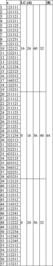
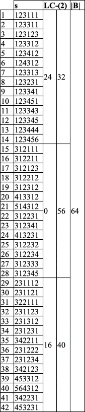
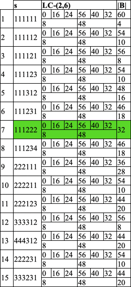
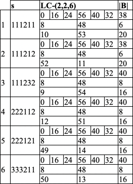
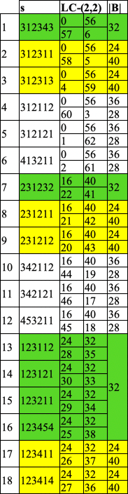
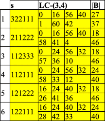
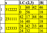
Figure 9: All the possible block-sequential attractors of Boolean automata network $\Psi$ defined in Figure 8.

In view of the results depicted in Figure 9, we could say that network $\Psi$ is robust to block-sequential update modes. Indeed, regardless of the update mode used, fixed points never appear. Now, if we consider the parallel dynamics of $\Psi$ which is of type LC-$(2,6)$, it is interesting to ask if we can make small modifications to $\Psi$ while maintaining its graph and type of local functions in order to obtain another network whose parallel dynamics is also of type LC-$(2,6)$. A first step in doing this and finding networks like $\Psi$ that eventually have no fixed points is considering networks whose interaction graphs contain at least one negative edge, as stated by the following proposition.

Proposition 1.

Let $f$ be a Boolean automata network. Let $g$ be a Boolean automata network whose interaction graph is the same as that of $f$. If a block-sequential dynamics of $g$ has no fixed points, then neither do its other block-sequential dynamics, and at least one of the edges of $g$ is negative.

Proof.

Consider $f$ and $g$ two distinct Boolean automata networks as stated just above. Let $\mu$ be a block-sequential update mode such that the dynamics of $g$ with $\mu$ has no fixed point. Since fixed points are invariant regardless of the block-sequential update mode [32], then it is direct that the other block-sequential dynamics do not have any either. Now, suppose that all edges of $g$ are positive. Since the type of local functions are of type and/or, then the all-$0$ and all-$1$ configurations are fixed points of $g$, which is a contradiction. ∎

Proposition 1 establishes a starting condition to eventually find the networks having at least one negative edge. However, in the framework of our model $\Psi$, it is easy to do an exhaustive search by simulation and show that there are no other like $\Psi$. Indeed, without entering into the details, all possible and/or Boolean automata networks having an interaction graph which conserves the structure of that $\Psi$ admit parallel dynamics which include asymptotically either fixed points or limit cycles of other type.

$\alpha:B^{6}\to B^{6}$

$\alpha(x)=\left\{\begin{array}[]{l}\alpha_{1}(x)=x_{3}\\ \alpha_{2}(x)=x_{1}\\ \alpha_{3}(x)=x_{2}\lor x_{4}\\ \alpha_{4}(x)=\neg x_{3}\land x_{6}\\ \alpha_{5}(x)=x_{4}\\ \alpha_{6}(x)=x_{5}\\ \end{array}\right.$

$\beta:B^{6}\to B^{6}$

$\beta(x)=\left\{\begin{array}[]{l}\beta_{1}(x)=x_{3}\\ \beta_{2}(x)=\neg x_{1}\\ \beta_{3}(x)=x_{2}\lor x_{4}\\ \beta_{4}(x)=\neg x_{3}\land x_{6}\\ \beta_{5}(x)=x_{4}\\ \beta_{6}(x)=\neg x_{5}\\ \end{array}\right.$

$\gamma:B^{6}\to B^{6}$

$\gamma(x)=\left\{\begin{array}[]{l}\gamma_{1}(x)=x_{3}\\ \gamma_{2}(x)=\neg x_{1}\\ \gamma_{3}(x)=x_{2}\lor\neg x_{4}\\ \gamma_{4}(x)=x_{3}\land x_{6}\\ \gamma_{5}(x)=x_{4}\\ \gamma_{6}(x)=x_{5}\\ \end{array}\right.$

$\delta:B^{6}\to B^{6}$

$\delta(x)=\left\{\begin{array}[]{l}\delta_{1}(x)=x_{3}\\ \delta_{2}(x)=x_{1}\\ \delta_{3}(x)=x_{2}\lor\neg x_{4}\\ \delta_{4}(x)=x_{3}\land x_{6}\\ \delta_{5}(x)=x_{4}\\ \delta_{6}(x)=x_{5}\\ \end{array}\right.$

$\zeta:B^{6}\to B^{6}$

$\zeta(x)=\left\{\begin{array}[]{l}\zeta_{1}(x)=x_{3}\\ \zeta_{2}(x)=\neg x_{1}\\ \zeta_{3}(x)=x_{2}\lor\neg x_{4}\\ \zeta_{4}(x)=x_{3}\land x_{6}\\ \zeta_{5}(x)=x_{4}\\ \zeta_{6}(x)=\neg x_{5}\\ \end{array}\right.$

$\eta:B^{6}\to B^{6}$

$\eta(x)=\left\{\begin{array}[]{l}\eta_{1}(x)=x_{3}\\ \eta_{2}(x)=\neg x_{1}\\ \eta_{3}(x)=x_{2}\lor x_{4}\\ \eta_{4}(x)=x_{3}\land x_{6}\\ \eta_{5}(x)=x_{4}\\ \eta_{6}(x)=x_{5}\\ \end{array}\right.$

Figure 10: Six and/or Boolean automata networks with their associated interactions which conserve both the type of local functions of $\Psi$ and the underlying structure of that of $\Psi$.

As an illustration, Figure 10 depicts six Boolean automata networks together with their interaction graphs which are small modifications of $\Psi$. If we compute all the block-sequential dynamics of each of these networks, we can observe the following differences with those of $\Psi$:

• The parallel dynamics of $\alpha$ and $\delta$ includes two fixed points and there exist other dynamics with no limit cycles;

• The parallel dynamics of $\beta$ and $\zeta$ has no fixed point bu has a limit cycle of length $5$;

• The parallel dynamics of $\gamma$ and $\eta$ includes one fixed point and there exist other dynamics with no limit cycles.

3.3 Discussion around a specific intricate update mode

We have already seen view from results of Section 3.2 that Boolean automata network $\Psi$ related to hereditary angioedema is robust because, regardless of the block- sequential update mode, fixed points never appear, which is coherent with the empiric observation that most of genes involved the disease have a periodic expression due in part to the chromatin clock and circadian rhythms [43].

Some genes are updated systematically together under the control of the chromatin clock. In order to achieve a systematic plan of numerical experience, we shall compare the block-sequential update modes related to $\Psi$ studied in Section 3.2 to an intricate update mode, for which we consider that automata $3$ (modeling SP1) and $4$ (modeling F12) tends to actively express their protein. This intricate update mode is a specific block-parallel update mode which has been inspired by F. Robert, who defined the notion of interactions between two Boolean automata network of size $2$ as follows. Consider two Boolean automata networks of size $2$ whose global functions are $f$ and $g$. Interactions between $f$ and $g$ can be of four types [12]:

• Sequential dependence: two networks $f$ and $g$ of size $2$ are said to be sequential-dependent when

  $$f_{1}(x_{1}x_{2})=f_{0}(g_{0}(x_{1}x_{2})x_{2}),g_{1}(x_{1}x_{2})=g_{0}(x_{1}f_{1}(x_{1}x_{2})),\dots,\\ f_{i}(x_{1}x_{2})=f_{i-1}(g_{i-1}(x_{1}x_{2})x_{2}),g_{i}(x_{1}x_{2})=g_{i-1}(x_{1}f_{i}(x_{1}x_{2}))\text{,}$$

  or conversely when

  $$g_{1}(x_{1}x_{2})=g_{0}(f_{0}(x_{1}x_{2})x_{2}),f_{1}(x_{1}x_{2})=f_{0}(x_{1}g_{1}(x_{1}x_{2})),\dots,\\ g_{i}(x_{1}x_{2})=g_{i-1}(f_{i-1}(x_{1}x_{2})x_{2}),f_{i}(x_{1}x_{2})=f_{i-1}(x_{1}g_{i}(x_{1}x_{2}))\text{.}$$

• Parallel dependence: two networks $f$ and $g$ of size $2$ are said to be parallel-dependent when

  $$f_{1}(x_{1}x_{2})=f_{0}(g_{0}(x_{1}x_{2})x_{2}),g_{1}(x_{1}x_{2})=g_{0}(x_{1}f_{0}(x_{1}x_{2})),\dots,\\ f_{i}(x_{1}x_{2})=f_{i-1}(g_{i-1}(x_{1}x_{2})x_{2}),g_{i}(x_{1}x_{2})=g_{i-1}(x_{1}f_{i-1}(x_{1}x_{2}))\text{,}$$

  or conversely when

  $$g_{1}(x_{1}x_{2})=g_{0}(f_{0}(x_{1}x_{2})x_{2}),f_{1}(x_{1}x_{2})=f_{0}(x_{1}g_{0}(x_{1}x_{2})),\dots,\\ g_{i}(x_{1}x_{2})=g_{i-1}(f_{i-1}(x_{1}x_{2})x_{2}),f_{i}(x_{1}x_{2})=f_{i-1}(x_{1}g_{i-1}(x_{1}x_{2}))\text{.}$$

• Sequential opposition: two networks $f$ and $g$ of size $2$ are said to be sequential-opposed when

  $$f_{1}(x_{1}x_{2})=f_{0}(\neg g_{0}(x_{1}x_{2})x_{2}),g_{1}(x_{1}x_{2})=g_{0}(x_{1}\neg f_{1}(x_{1}x_{2})),\dots,\\ f_{i}(x_{1}x_{2})=f_{i-1}(\neg g_{i-1}(x_{1}x_{2})x_{2}),g_{i}(x_{1}x_{2})=g_{i-1}(x_{1}\neg f_{i}(x_{1}x_{2}))\text{.}$$

  or conversely when

  $$g_{1}(x_{1}x_{2})=g_{0}(\neg f_{0}(x_{1}x_{2})x_{2}),f_{1}(x_{1}x_{2})=f_{0}(x_{1}\neg g_{1}(x_{1}x_{2})),\dots,\\ g_{i}(x_{1}x_{2})=g_{i-1}(\neg f_{i-1}(x_{1}x_{2})x_{2}),f_{i}(x_{1}x_{2})=f_{i-1}(x_{1}\neg g_{i}(x_{1}x_{2}))\text{.}$$

• Parallel opposition: two networks $f$ and $g$ of size $2$ are said to be parallel-opposed when:

  $$f_{1}(x_{1}x_{2})=f_{0}(\neg g_{0}(x_{1}x_{2})x_{2}),g_{1}(x_{1}x_{2})=g_{0}(x_{1}\neg f_{0}(x_{1}x_{2})),\dots,\\ f_{i}(x_{1}x_{2})=f_{i-1}(\neg g_{i-1}(x_{1}x_{2})x_{2}),g_{i}(x_{1}x_{2})=g_{i-1}(x_{1}\neg f_{i-1}(x_{1}x_{2}))\text{,}$$

  or conversely when

  $$g_{1}(x_{1}x_{2})=g_{0}(\neg f_{0}(x_{1}x_{2})x_{2}),f_{1}(x_{1}x_{2})=f_{0}(x_{1}\neg g_{0}(x_{1}x_{2})),\dots,\\ g_{i}(x_{1}x_{2})=g_{i-1}(\neg f_{i-1}(x_{1}x_{2})x_{2}),f_{i}(x_{1}x_{2})=f_{i-1}(x_{1}\neg g_{i-1}(x_{1}x_{2}))\text{.}$$

We can also write for the sequential dependence between automata networks of size $n$:

$$g_{0}=g,f_{0}=f,g_{1}=g_{0}(f_{0,I}K),f_{1}=f_{0}(Ig_{1,K}),\dots,\\ g_{i}=g_{i-1}(f_{i-1,I}K),f_{i}=f_{i-1}(Ig_{i-1,K}),\dots,\\ g_{n}=g_{n-1}(f_{n-1,I}K),f_{n}=f_{n-1}(Ig_{n-1,K})\text{,}$$

where $I$ and $K$ $\subseteq\{1,\dots,n\}$ and $I$ (resp. $K$) is the identity on $x_{I\setminus K}=\{x_{i}\}_{i\in I\setminus K}$ (resp. $x_{K\setminus I}=\{x_{j}\}_{jK\setminus I}$, and $f_{0,I}$ (resp. $g_{1,K}$) is the projection of $f_{0}$ on $I\setminus K$ (resp. $g_{1}$ on $K\setminus I$).

In our case, $n=6$ and $f$ and $g$ are defined by the logic equations of the Figure 8. Complex biological networks [11] fall within the general framework above, provided that more information is available on the role of the chromatin clock which regulates the timing of updating of their components. This constitutes an additional degree of complexity because certain histones involved in this chromatin regulation have transcription factors involved in the networks whose expression is controlled by these histones.

F. Robert studied systematically the corresponding dynamics and proved the following proposition in the case of a network of size $2$, when $I\cap K\neq\emptyset$.

Proposition 2.

1. Sequential and parallel dependence (resp. opposition) rules give same fixed points.

2. The update mode defined by the sequential (resp. parallel) opposition between $\neg f$ and $\neg g$ gives the complementary dynamics to that given by the update mode defined by the sequential (resp. parallel) dependence between $f$ and $g$.

Figure 11: Dynamics of BAN₆ $f$ presented in Figure 8 according to the intricate block-parallel update mode $(\{1,2,3,4\},\{3,4,5,6\})$ which exhibits a unique limit cycle composed of dark configurations. The $64$ configurations are represented thanks to their ten-base encoding for the sake of concision.

We can remark on Figure 11 that there is a unique limit cycle LC, which is of length $4$ for the intricate updating mode $(\{1,2,3,4\},\{3,4,5,6\})$ which implements the ideas behind the sequential dependence defined above, where $LC=(100000,000000,011000,111000)$. This limit cycle corresponds to the most frequent asymptotic behavior the non-intricate block- sequential dynamics (see Figure 9), which reinforces the robust character of the genetic network, considered as the core of the regulation involved in the hereditary angioedema.

If there is a change in the expression of the genes involved in this disease, it will not be due to a change in the clock (for example, the chromatin clock or the circadian clock that controls it), but rather, which confirms the currently accepted explanation, to an endogenous hormonal influence (estrogen impregnation) or to exogenous elements triggering attacks of a physical nature (influence of cold or exercise), dietary (allergy) or pathological (stress; surgical or drug therapy; common illnesses such as colds and flu; insect bites, etc.).

4 Conclusion

We have introduced a new variety of periodic update modes, the intricate update modes, which generalizes that of block-parallel update modes by inclusion. Indeed, from the mathematical standpoint, block-parallel updates modes are modes with local repetitions of updates over their period which are derived from their specific characterization as partitioned orders whereas intricate modes admit local repetitions of updates with no specific structural constraint. Moreover, from the biological modeling standpoint, basing ourselves on the wish to make advances on the understanding of the genetic regulation governing hereditary angioedema, we developed a simplified version of the a known genetic regulatory network for this disease, which conserves only the major players in regulation of gene expression. From this network and its underlying Boolean automata network model, we emphasized the strong robustness of our model with respect to block-sequential update, by showing that none of its asymptotic behaviors are fixed points which is coherent with empiric observation that the expression of most of the genes involved in hereditary angioedema follows periodical paces. The, we developed an intricate update mode, which is an alternating block-parallel update mode which have been introduced recently in [14] in the framework of biological modeling [40], and highlight that such modes could model the action of Zeitgebers. Here, the intricate update mode is particular in the sense that it is structurally defined such that a core subnetwork of two automata (or genes) is constantly updated and acts on two other subnetworks which alternate their updatings. More precisely, the automata of the model are thus updated according to distinct schedules, some being updated at each iteration and others being updated at lower frequencies (every other time, in the chosen example). We highlighted that this intricate update mode captures the main block-sequential limit cycle, i.e. the one which is most often reached with block-sequential update modes and which admits an attraction basin as big as possible, namely composed of all the configurations.

In the application to Boolean networks of genetic regulation, in the absence of precise information on the mode of updating the states of the nodes of the network (i.e. the expression of the genes involved), it is necessary to examine the consequences of a change of mode on the dynamics of the network (possible change in the number, nature and size of the basins of attraction of its attractors). If the characteristics of the attractors are invariant in a change of update mode, the network is said to be robust. In that case, the choice of a dynamics rather an other one is less crucial for the practical consequences of the discrete modeling of the expression of the genes studied, in particular to explain the genesis of a pathology of familial origin involving a set of well-identified interacting genes, which is the case in the disease taken as an example, namely the hereditary angioedema.

Acknowledgements

The authors acknowledge C. Drouet for helpul discussion about hereditary angioedema. This work was partially funded by the ANR-24-CE48-7504 “ALARICE” project (S.S.), the HORIZON-MSCA-2022-SE-01 101131549 “ACANCOS” project (E.G., S.S.), the STIC AmSud 22-STIC-02 “CAMA” project (E.G., M.M.-M., S.S.), the FONDECYT/ANID Regular 1250984 (E.G., M.M.-M.) and the ANID-MILENIO-NCN2024 103 (E.G.) project.

References

- [1] Julio Aracena, Jacques Demongeot, Éric Fanchon, and Marco Montalva. On the number of different dynamics in Boolean networks with deterministic update schedules. Mathematical Biosciences, 242:188–194, 2013.
- [2] Julio Aracena, Jacques Demongeot, Éric Fanchon, and Marco Montalva. On the number of update digraphs and its relation with the feedback arc sets and tournaments. Discrete Applied Mathematics, 161:1345–1355, 2013.
- [3] Julio Aracena, Éric Fanchon, Marco Montalva, and Mathilde Noual. Combinatorics on update digraphs in Boolean networks. Discrete Applied Mathematics, 159:401–409, 2011.
- [4] Julio Aracena, Eric Goles, Andres Moreira, and Lilian Salinas. On the robustness of update schedules in Boolean networks. Biosystems, 97:1–8, 2009.
- [5] Nam P. Bhatia and Giorgio P. Szegö. Dynamical Systems: Stability Theory and Applications, volume 35 of Lecture Notes in Mathematics. Springer, 1967.
- [6] George D. Birkhoff. Dynamical Systems, volume 9 of AMS Colloquium Publications. American Mathematical Society, 1927.
- [7] Rufus Bowen. -limit sets for axiom A diffeomorphisms. Journal of Differential Equations, 18:333–339, 1975.
- [8] Charles Conley. Isolated invariant sets and the Morse index, volume 38 of Regional Conference Series in Mathematics. American Mathematical Society, 1978.
- [9] Thomas H. Cormen, Charles E. Leiserson, Ronald L. Rivest, and Clifford Stein. Introduction to Algorithms. MIT Press and McGraw-Hill, 2nd edition, 2001.
- [10] Michel Cosnard and Jacques Demongeot. Attracteurs : une approche déterministe. Comptes rendus de l’Académie des sciences. Série 1, Mathématique, 300:551–556, 1985.
- [11] Jacques Demongeot, Abdoul Khadir Diallo, Hana Hazgui, Mariem Jelassi, Fatine Kelloufi, and Houssem ben Khalfallah. Boolean networks with intricate updating mode: application to genetic regulatory networks involved in familial diseases. Preprint, 2025.
- [12] Jacques Demongeot. Seven things I know about them, volume 42 of Emergence, Complexity and Computation. Springer, 2022.
- [13] Jacques Demongeot, Adrien Elena, and Sylvain Sené. Robustness in regulatory networks: a multi-disciplinary approach. Acta Biotheoretica, 56:27–49, 2008.
- [14] Jacques Demongeot and Sylvain Sené. About block-parallel Boolean networks: a position paper. Natural Computing, 19:5–13, 2020.
- [15] Isabel Donoso Leiva, Eric Goles, Martín Ríos-Wilson, and Sylvain Sené. Asymptotic (a)synchronism sensitivity and complexity of elementary cellular automata. In LATIN 2024: Theoretical Informatics, volume 14579 of Lecture Notes in Computer Science, pages 272–286, Springer, 2024.
- [16] Luis Garrido and Carles Simó. Some ideas about strange attractors. In Dynamical Systems and Chaos, volume 179 of Lecture Notes in Physics, pages 1–28, Springer, 1983.
- [17] Eric Goles, Marco Montalva-Medel, Stephanie MacLean, and Henning S. Mortveit. Block invariance in a family of elementary cellular automata. Journal of Cellular Automata, 13:15–32, 2018.
- [18] Eric Goles, Marco Montalva-Medel, Henning S. Mortveit, and Salvador Ramírez-Flandes. Block invariance in elementary cellular automata. Journal of Cellular Automata, 10:119–135, 2015.
- [19] Eric Goles and Jorge Olivos. Periodic behaviour of generalized threshold functions. Discrete Mathematics, 30:187–189, 1980.
- [20] John Guckenheimer and Philip Holmes. Nonlinear Oscillations, Dynamical Systems, and Bifurcations of Vector Fields, volume 42 of Applied Mathematical Sciences. Springer, 1983.
- [21] Inman Harvey and T Bossomaier. Time out of joint, attractors in asynchronous random Boolean networks. In ECAL 1997: Fourth European Conference on Artificial Life, pages 67–75, MIT Press, 1997.
- [22] John J. Hopfield. Neural networks and physical systems with emergent collective computational abilities. Proceedings of the National Academy od Sciences of the United States of America, 79:2554–2558, 1982.
- [23] Stuart A. Kauffman. Metabolic stability and epigenesis in randomly constructed genetic nets. Journal of Theoretical Biology, 22:437–467, 1969.
- [24] Stephen C. Kleene. Representation of events in nerve nets and finite automata. Princeton University Press, 1951.
- [25] Georges-Louis Leclerc de Buffon. Histoire naturelle, générale et particulière, avec la description du Cabinet du Roy. Imprimerie Royale, 1749.
- [26] Warren S. McCulloch and Walter Pitts. A logical calculus of the ideas immanent in nervous activity. The Bulletin of Mathematical Biophysics, 5:115–133, 1943.
- [27] Loïc Paulevé and Sylvain Sené. Boolean networks and their dynamics: the impact of updates. Wiley, 2022.
- [28] Kévin Perrot, Marco Montalva-Medel, Pedro P. Balbi de Oliveira, and Eurico L.P. Ruivo. Maximum sensitivity to update schedules of elementary cellular automata over periodic configurations. Natural Computing, 19:51–90, 2020.
- [29] Kévin Perrot, Sylvain Sené, and Léah Tapin. Combinatorics of block-parallel automata networks. In SOFSEM 2024: Theory and Practive of Computer Science, volume 14519 of Lecture Notes in Computer Science, pages 442–455, Springer, 2024.
- [30] Kévin Perrot, Sylvain Sené, and Léah Tapin. Complexity of Boolean automata networks under block-parallel update modes. In 3rd Symposium on Algorithmic Foundations of Dynamic Networks (SAND 2024), volume 292 of Leibniz International Proceedings in Informatics, pages 19:1–19:19, Schloss Dagstuhl – Leibniz-Zentrum für Informatik, 2024.
- [31] Mustapha Rachdi, Jules Waku, Hana Hazgui, and Jacques Demongeot. Entropy as a robustness marker in genetic regulatory networks. Entropy, 22:260, 2020.
- [32] François Robert. Discrete Iterations: A Metric Study, volume 6 of Springer Series in Computational Mathematics. Springer, 1986.
- [33] David Ruelle. Small random perturbations of dynamical systems and the definition of attractors. Communications in Mathematical Physics, 82:137–151, 1981.
- [34] Eurico L.P. Ruivo, Pedro P. Balbi, Marco Montalva-Medel, and Kévin Perrot. Maximum sensitivity to update schedules of elementary cellular automata over infinite configurations. Information and Computation, 274:104538, 2020.
- [35] Ya G. Sinai. The stochasticity of dynamical systems. Selecta Mathematica Sovietica, 1:100–119, 1981.
- [36] Stephen Smale. Differentiable dynamical systems. Bulletin of the American Mathematical Society, 73:747–817, 1967.
- [37] Robert E. Tarjan. Depth-first seach and linear graph algorithms. SIAM Journal on Computing, 1:146–160, 1972.
- [38] René Thom. Stabilité structurelle et morphogenèse. InterEditions, 1972.
- [39] René Thomas. Boolean formalization of genetic control circuits. Journal of Theoretical Biology, 42:563–585, 1973.
- [40] Richard Tomassone, Catherine Dervin, and Jean-Pierre Masson. Biométrie : Modélisation de phénomènes biologiques. Masson, 1993.
- [41] Denis Vincent, Faidra Parsopoulou, Ludovic Martin, Christine Gaboriaud, Jacques Demongeot, Gedeon Loules, Sascha Fischer, Sven Cichon, Anastasios E. Germenis, Arije Ghannam, and Christian Drouet. Hereditary angioedema with normal C1 inhibitor associated with carboxypeptidase N deficiency. Journal of Allergy and Clinical Immunology: Global, 3:100223, 2024.
- [42] Robert F. Williams. Expanding attractors. Publications Mathématiques de l’Institut des Hautes Études Scientifiques, 43:169–203, 1974.
- [43] Shan Zhang, Peiqi Huang, Huijuan Dai, Qing Li, Lipeng Hu, Jing Peng, Shuheng Jiang, Yaqian Xu, Ziping Wu, Huizhen Nie, Zhigang Zhang, Wenjin Yin, Xueli Zhang, and Jinsong Lu. TIMELESS regulates sphingolipid metabolism and tumor cell growth through Sp1/ACER2/S1P axis in ER-positive breast cancer. Cell Death & Disease, 11:892, 2020.