ABBA: Highly Expressive Hadamard Product Adaptation for Large Language Models

Abstract

Large Language Models have demonstrated strong performance across a wide range of tasks, but adapting them efficiently to new domains remains a key challenge. Parameter-Efficient Fine-Tuning (PEFT) methods address this by introducing lightweight, trainable modules while keeping most pre-trained weights fixed. The prevailing approach, LoRA, models updates using a low-rank decomposition, but its expressivity is inherently constrained by the rank. Recent methods like HiRA aim to increase expressivity by incorporating a Hadamard product with the frozen weights, but still rely on the structure of the pre-trained model. We introduce ABBA, a new PEFT architecture that reparameterizes the update as a Hadamard product of two independently learnable low-rank matrices. In contrast to prior work, ABBA fully decouples the update from the pre-trained weights, enabling both components to be optimized freely. This leads to significantly higher expressivity under the same parameter budget. We formally analyze ABBA’s expressive capacity and validate its advantages through matrix reconstruction experiments. Empirically, ABBA achieves state-of-the-art results on arithmetic and commonsense reasoning benchmarks, consistently outperforming existing PEFT methods by a significant margin across multiple models. Our code is publicly available at: https://github.com/CERT-Lab/abba.

1 Introduction

Large Language Models (LLMs) have become the backbone of modern NLP systems Radford2021LearningTV ; Kirillov2023SegmentA ; achiam2023gpt ; touvron2023llama-2 ; team2023gemini ; yang2024qwen2 ; team2025gemma , demonstrating strong generalization across a wide range of tasks bubeck2023sparks ; Hao_Song_Dong_Huang_Chi_Wang_Ma_Wei_2022 . However, adapting these models to new tasks typically requires full fine-tuning (FT), which is computationally and memory intensive. Parameter-Efficient Fine-Tuning (PEFT) methods address this challenge by introducing a small number of trainable parameters while keeping the majority of model weights frozen lora ; Liu_Wang_Yin_Molchanov_Wang_Cheng_Chen_2024 ; LoRA-XS . Among PEFT approaches, Low-Rank Adaptation (LoRA) lora is the most widely adopted due to its simplicity and effectiveness. It models the weight update $\Delta W$ as the product of two low-rank matrices, providing a compact parameterization. However, this formulation inherently constrains updates to a low-dimensional subspace, limiting expressivity. Several extensions attempt to overcome this limitation: LoRA-XS LoRA-XS restricts updates to a frozen, SVD-derived subspace and training only a small higher-rank intermediary matrix while DoRA Liu_Wang_Yin_Molchanov_Wang_Cheng_Chen_2024 modifies only the directional component of the weights via low-rank updates. Despite these architectural variations, all retain LoRA’s core constraint: updates remain strictly low-rank and limited in expressivity.

HiRA huang2025hira addresses LoRA’s limited expressivity by applying a Hadamard product between a low-rank update and the frozen pre-trained weights $W_{0}$, enabling updates that can, in principle, attain full rank. However, HiRA’s expressivity remains tightly coupled to $W_{0}$, as the learned adapters merely modulate the pre-trained weights rather than generating the full update independently. For example, if the target update equals $\mathrm{diag}(W_{0})$, HiRA must learn adapters that approximate the identity matrix, an orthonormal structure that is challenging for low-rank modules to represent accurately (Figure 2).

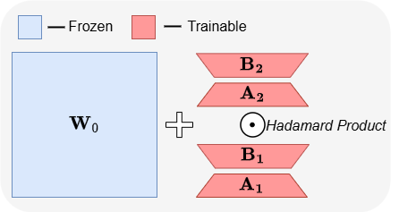
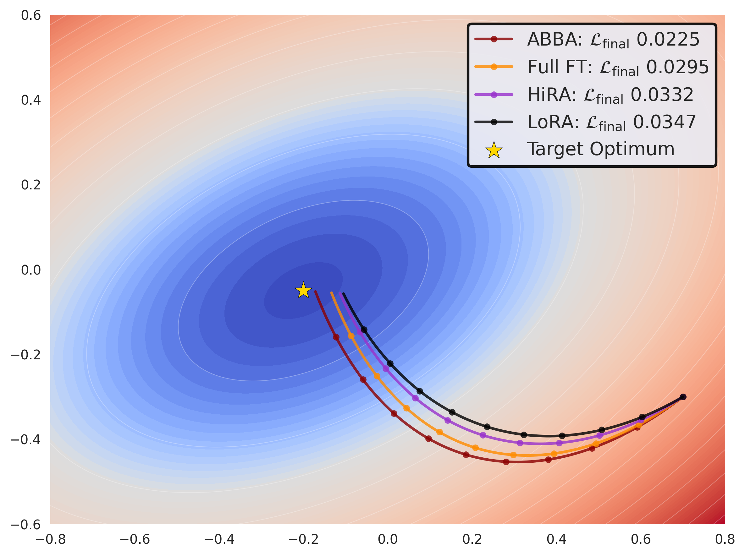
Figure 1: Left: Illustration of ABBA’s parameterization, where the update is expressed as the Hadamard product of two learnable low-rank matrices. Right: A toy experiment demonstrating ABBA’s optimization behavior. We first train a 2-layer MLP to classify the first 8 MNIST digits, then fine-tune it to recognize the last 2. ABBA converges faster and achieves better final performance.

In this work, we introduce ABBA, a novel architecture framework that reparameterizes the weight update as the Hadamard product of two fully learnable low-rank matrices (see Figure 1). Each component is independently formed via a low-rank decomposition ($B_{1}A_{1}$ and $B_{2}A_{2}$), resulting in a highly expressive update while maintaining parameter counts. Unlike HiRA, ABBA is fully decoupled from the pretrained weights $W_{0}$, allowing both components to be optimized without structural constraints. The name ABBA reflects the four low-rank matrices that define the architecture.

We support our formulation with both theoretical and empirical evidence. First, we analyze expressivity through a matrix reconstruction task, where Hadamard-structured updates consistently outperform standard LoRA decompositions under the same parameter budget (Figure 2). This demonstrates that ABBA can represent a broader class of updates than LoRA within identical constraints. Next, a toy MNIST experiment (Figure 1) shows that ABBA converges to a solution significantly closer to the true optimum compared to LoRA and HiRA, indicating that its increased expressivity is also practically accessible during learning. We present an exact reformulation of the ABBA update using Khatri–Rao matrix factorization, enabling efficient implementation without approximation. Empirically, ABBA consistently outperforms existing PEFT methods across a broad range of tasks and models, all within the same or lower parameter budget. Our key contributions are summarized as:

• We propose ABBA, a novel PEFT architecture that models the weight update as the Hadamard product of two independently learnable low-rank matrices. This formulation enables highly expressive, high-rank updates while preserving strict parameter efficiency.

• We provide theoretical and empirical analyses of ABBA’s expressivity, showing that Hadamard-based decomposition consistently outperforms standard low-rank methods in matrix reconstruction.

• We introduce an exact and efficient reformulation of ABBA using Khatri–Rao factorization, enabling scalable and practical implementation without compromising expressivity.

• Through extensive experiments on four models across arithmetic and commonsense reasoning tasks, we demonstrate that ABBA achieves state-of-the-art performance, significantly outperforming existing PEFT methods under equal or lower parameter budgets.

2 Methodology

2.1 Preliminaries

Full Fine-Tuning. Given a pre-trained weight matrix $W_{0}\in\mathbb{R}^{m\times n}$, full FT updates all parameters via $W=W_{0}+\Delta W$, introducing $m\times n$ trainable parameters per layer. This quickly becomes impractical due to the high memory and compute overhead.

LoRA lora . LoRA mitigates this by modeling the update as a low-rank decomposition: $\Delta W=sBA$, where $B\in\mathbb{R}^{m\times r}$, $A\in\mathbb{R}^{r\times n}$, and $s$ is a scaling factor. This reduces the number of trainable parameters to $r(m+n)$, with $r\ll\min(m,n)$. LoRA can represent any update of rank at most $r$, but cannot express higher-rank updates. Moreover, the projected gradient onto the weight space is also low-rank. While effective for simpler tasks, this limitation becomes significant in settings requiring high-rank updates or gradients LoRA-Pro ; ponkshe2025initializationusingupdateapproximation .

HiRA (Hadamard High-Rank Adaptation)  huang2025hira . HiRA lifts LoRA’s rank limitation by modulating its low-rank update with an element-wise (Hadamard) product with the frozen pre-trained weight $W_{0}$:

$$\Delta W=W_{0}\odot(BA),\quad\text{where}\odot\text{denotes the Hadamard product}.$$ (1)

This leverages the property that the Hadamard product of two matrices $W_{1}$ and $W_{2}$ with ranks $r_{1}$ and $r_{2}$ respectively satisfies $\operatorname{rank}(W_{1}\odot W_{2})\leq r_{1}\cdot r_{2}$. Thus, HiRA can produce updates of rank up to $r_{0}r$, where $r_{0}=\operatorname{rank}(W_{0})$, potentially addressing the low-rank limitation of LoRA. Additionally, the gradient projected onto $W$ is no longer low-rank. However, higher rank does not necessarily imply greater expressivity. Because HiRA’s update is element-wise tied to $W_{0}$, it is restricted to a subspace defined by the pre-trained weights. This dependence can hinder generalization, especially in out-of-domain scenarios. As shown in Section 2.4, HiRA reduces reconstruction error over LoRA only when the element-wise ratio of the oracle update to $W_{0}$ is itself low-rank.

2.2 Improving the Expressivity of HiRA

A natural way to overcome HiRA’s expressivity constraint is to make the matrix $W_{h}$ learnable:

$$\Delta W=W_{h}\odot(BA),\qquad\text{where }W_{h}\in\mathbb{R}^{m\times n}\ \text{is trainable}.$$ (2)

However, this reintroduces the full $m\times n$ parameter cost of $W_{h}$, negating LoRA’s core efficiency advantage. Even if $W_{h}$ is fixed but not equal to $W_{0}$, the additional memory required to store it significantly increases the overhead. In contrast, HiRA sets $W_{h}=W_{0}$, which is already stored, thereby preserving LoRA’s parameter and memory efficiency. This raises a critical question:

Can we achieve greater expressivity and high-rank learning while maintaining the parameter and memory efficiency of LoRA?

Importantly, we note that full-rank updates are not always necessary. Moreover, $W_{h}$ itself does not need to be full-rank. Since any $m\times n$ matrix has rank at most $r_{0}=\min(m,n)$, a modulation matrix with rank above $r_{0}/r$ offers no additional expressivity for the Hadamard product.

2.3 ABBA: Highly Expressive and High Rank, Yet Efficient

As discussed above, high-rank updates do not require $W_{h}$ to be full-rank. Leveraging this insight, we reparameterize $W_{h}$ as the Hadamard product of two independently learnable low-rank matrices, resulting in the following formulation:

$$\Delta W=s(B_{1}A_{1})\odot(B_{2}A_{2}),$$ (3)

where $B_{1}\in\mathbb{R}^{m\times r_{1}},\;A_{1}\in\mathbb{R}^{r_{1}\times n}$ and $B_{2}\in\mathbb{R}^{m\times r_{2}},\;A_{2}\in\mathbb{R}^{r_{2}\times n}$, with $r_{1},r_{2}\ll\min(m,n)$ and $s$ is a scaling factor for stability. This parameterization introduces only $(r_{1}+r_{2})(m+n)$ parameters, significantly fewer than full FT, and achieves an effective rank up to $r_{1}r_{2}$. To maximize expressivity under a fixed parameter budget, we set $r_{1}=r_{2}$, as further supported by empirical results in Section 4.2. This preserves HiRA’s ability to produce high-rank updates while improving expressivity, since all four matrices are independently learned. For fair comparison with LoRA and other PEFT baselines, we match parameter counts by setting $r_{1}=r_{2}=r/2$, so that ABBA and other methods use equivalent parameter budgets.

Initialization of ABBA Adapters.

HiRA fixes the modulation matrix as $W_{h}=W_{0}$, directly tying the update to the pretrained weights. In contrast, ABBA makes this matrix fully learnable by reparameterizing it as $W_{h}=B_{1}A_{1}$. We initialize the first adapter pair $(B_{1},A_{1})$ using the top-$r_{1}$ components from a truncated SVD of $W_{0}$, and the second pair $(B_{2},A_{2})$ using the standard LoRA initialization: $B_{2}$ as zeros and $A_{2}$ with Kaiming uniform sampling.

$$U_{r_{1}},\Sigma_{r_{1}},V_{r_{1}}^{\top}\leftarrow\textbf{SVD}_{r_{1}}(W_{0}),$$ (4)

$$B_{1}\leftarrow U_{r_{1}}\Sigma_{r_{1}}^{1/2},\quad A_{1}\leftarrow\Sigma_{r_{1}}^{1/2}V_{r_{1}}^{\top},\quad B_{2}\leftarrow\mathbf{0},\quad A_{2}\leftarrow\mathcal{N}(0,\sigma^{2}).$$ (5)

By the Eckart–Young–Mirsky (EYM) theorem (eckart1936approximation, ; mirsky1960symmetric, ), the truncated SVD yields the optimal rank-$r_{1}$ approximation of $W_{0}$. This hybrid initialization anchors the update close to a meaningful low-rank subspace, while enabling the second adapter pair to explore task-specific directions during training. We validate the effectiveness of this strategy empirically in Section 4.1.

Making ABBA Memory-Efficient.

While ABBA is clearly parameter-efficient, analyzing its memory footprint during training is more subtle. In LoRA, the update $\Delta W=BA$ is applied as $\Delta Wx=B(Ax)$, allowing intermediate computations to remain low-rank. Only the activation $Ax\in\mathbb{R}^{r}$ and the adapter weights need to be stored additionally, avoiding the materialization of the full $m\times n$ matrix $BA$. In contrast, ABBA’s update $\Delta W=(B_{1}A_{1})\odot(B_{2}A_{2})$ poses a challenge. A naive implementation would require constructing both $B_{1}A_{1}$ and $B_{2}A_{2}$, followed by their elementwise product, resulting in the storage of multiple full $m\times n$ matrices. Moreover, unlike LoRA, the Hadamard product does not distribute over matrix–vector multiplication, so computing $B_{2}(A_{2}x)$ does not help incorporate the other matrices.

To address this, we use Theorem 1 to rewrite ABBA in a LoRA-like form: let $B_{\text{kr}}=B_{1}\odot_{r}B_{2}$ and $A_{\text{kr}}=(A_{1}^{\top}\odot_{r}A_{2}^{\top})^{\top}$. The update becomes $\Delta Wx=B_{\text{kr}}(A_{\text{kr}}x)$, avoiding any full-rank construction. This enables ABBA to match LoRA’s compute and memory efficiency, while offering significantly higher expressivity, and remain more efficient than variants like HiRA, as shown in Section 4.4.

Scaling Factor in the ABBA Update.

Theorem 1 reformulates the ABBA update as a Khatri–Rao product, giving it a superficially LoRA-like structure. rsLoRA rslora argues that stable LoRA training requires a scaling factor $\alpha_{\text{LoRA}}\propto 1/\sqrt{r}$. In ABBA, however, the Hadamard structure enables an effective rank of $r_{1}r_{2}$, suggesting an analogous scaling of $1/\sqrt{r_{1}r_{2}}$. Yet, since the parameterizations lie on fundamentally different manifolds, the justification used in rsLoRA does not directly apply. We formally derive the appropriate scaling for ABBA in Theorem 2, and support it with empirical evidence in Section 4.2.

2.4 Formalizing and Measuring Expressivity of ABBA

The expressivity of a matrix reparameterization can be evaluated by its ability to accurately reconstruct arbitrary target matrices, relative to alternative parameterizations.

LoRA and HiRA.

In LoRA, the weight update is modeled as a low-rank decomposition $\Delta W\approx BA$. For any matrix $M\in\mathbb{R}^{m\times n}$, the reconstruction error of this approximation is defined as:

$$\mathcal{E}(r)=\|M-BA\|_{F},$$ (6)

and is lower-bounded by the classical EYM theorem eckart1936approximation ; mirsky1960symmetric , which states that the optimal rank-$r$ approximation is given by the truncated SVD. Since a LoRA adapter of rank $r$ can only represent updates with rank at most $r$, EYM provides a theoretical minimum for $\mathcal{E}(r)$. LoRA achieves this bound exactly when the learned adapters align with the top singular components of $M$; otherwise, practical considerations such as suboptimal initialization may lead to a performance gap.

A similar bound can be derived for HiRA when the modulation matrix $W_{0}$ has all nonzero entries. In this case, the optimal Hadamard-structured approximation can be obtained by element-wise dividing $W$ by $W_{0}$, followed by applying truncated SVD to the resulting matrix. The expressivity advantage of HiRA over LoRA arises only if $\operatorname{rank}(\Delta W/W_{0})<\operatorname{rank}(\Delta W)$. Otherwise, for a general update $\Delta W$, HiRA has the same reconstruction error bound as LoRA, as characterized by the EYM theorem.

ABBA vs. LoRA: Reconstruction.

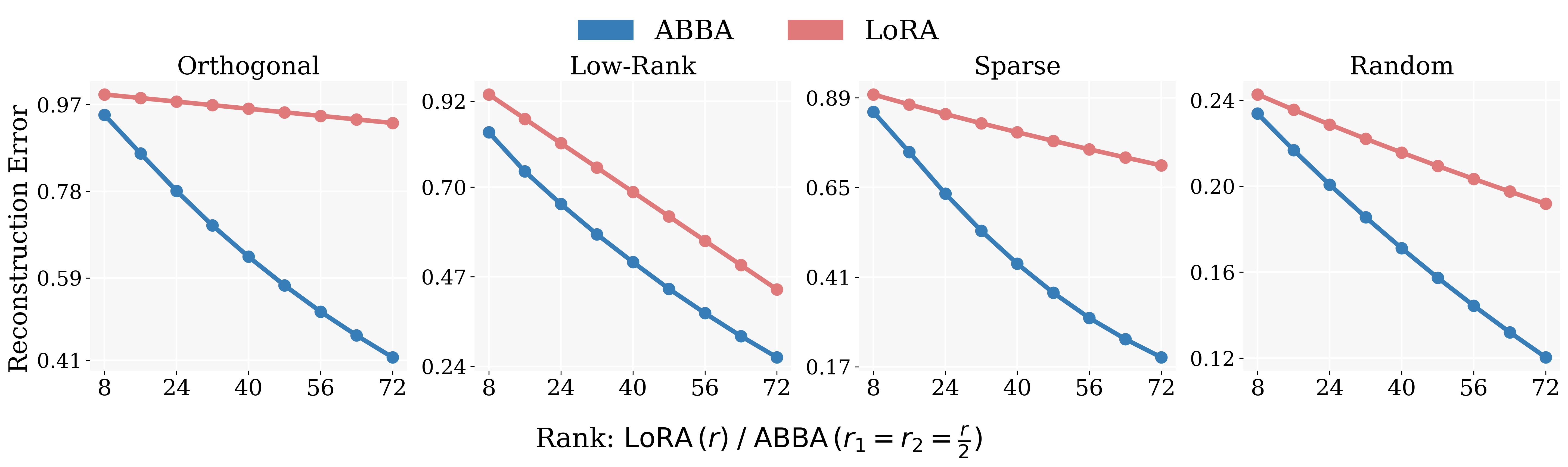
Figure 2: Empirical Reconstruction Errors. We compare ABBA and LoRA decompositions across various matrix types by measuring reconstruction error $\mathcal{E}(r)$ under equal parameter budgets. For each LoRA rank $r$, we set ABBA ranks to $r_{1}=r_{2}=r/2$ for a fair comparison. ABBA consistently achieves significantly lower reconstruction error than LoRA, across all matrix types.

Unlike SVD-based methods, ABBA does not admit a closed-form solution for its low-rank factors (see Appendix B for understanding why). We thus evaluate its expressivity by comparing the reconstruction error versus other methods. Given a target matrix $M\in\mathbb{R}^{m\times n}$, we define the reconstruction error for a method $X\in\{\text{LoRA},\text{ABBA}\}$ at rank $r$ as:
$E_{X,r}=\min_{M_{X,r}}\|M-M_{X,r}\|_{F}^{2},$ where the LoRA approximation is the truncated SVD $M_{\text{SVD},r}=U\Sigma_{r}V^{\top}$, and the ABBA approximation is given by $M_{\text{ABBA},r}=(B_{1}A_{1})\odot(B_{2}A_{2}).$

Previous work ciaperoni2024hadamard establishes a loose upper bound $E_{\text{ABBA},r}\leq E_{\text{LoRA},r}$, which holds trivially by setting one ABBA factor to the rank-$r$ SVD and the other to an all-ones matrix. Empirically, however, they observe a stronger trend: $E_{\text{ABBA},r}\lesssim E_{\text{LoRA},2r},$ which suggests that ABBA can match or outperform a rank-$2r$ SVD approximation using only rank $r$. However, this behavior is not guaranteed for arbitrary matrices, as the quality of reconstruction depends on the spectral properties and structure of the matrix. The only known theoretical comparison between the two is the bound: $E_{\text{LoRA},2r}-E_{\text{ABBA},r}\leq\sum_{i=2r+1}^{r^{2}}\sigma_{i}^{2},$ where $\sigma_{i}$ are the singular values of $M$. While this bound offers some insight, it is loose and does not guarantee a strict ordering between the reconstruction errors.

To better understand practical behavior, we empirically evaluate the reconstruction error of different parameterizations across diverse matrix types. As shown in Figure 2, the ABBA-based Hadamard reparameterization consistently achieves lower reconstruction error than standard LoRA, indicating greater expressivity. This aligns very well with prior work leveraging Hadamard structures for efficient and expressive matrix representations nam2022fedpara , further validating our formulation. Beyond these analyses, we also provide a probabilistic guarantee in Theorem 3 demonstrating when ABBA is likely to outperform LoRA in the presence of structured signals corrupted by noise.

2.5 Stability of the ABBA Update

The scaling factor $s_{\text{ABBA}}$ is critical in controlling the optimization dynamics of the ABBA update. It must be chosen carefully to scale appropriately with the ranks $r_{1}$ and $r_{2}$ of the underlying low-rank factors. If set too low, learning stagnates; if too high, training may diverge. While ABBA resembles LoRA in structure, its effective rank is $r_{1}r_{2}$, and the scaling behavior must reflect this increased capacity. Inspired by the scaling analysis in rsLoRA rslora and LoRA-GA wang2024lora , where stability is achieved under a complexity of $\mathcal{O}(1)$ with respect to rank, one might expect similar scaling for ABBA. However, since ABBA and LoRA inhabit different parameter spaces, these arguments do not transfer directly. To formalize this, we introduce the notion of rank-stability for ABBA in Definition 1, which ensures that forward and backward dynamics remain well-conditioned as $r_{1}$ and $r_{2}$ vary.

Definition 1 (Rank Stability of ABBA Adapters rslora ; wang2024lora ).

An ABBA adapter of the form $s_{\text{ABBA}}(B_{1}A_{1})\odot(B_{2}A_{2})$ is rank-stabilized if the following conditions hold:

1. If the $2^{\text{nd}}$ moment of the input is $\Theta_{r_{1},r_{2}}(1)$ in each entry with inputs being i.i.d, then the $2^{\text{nd}}$ moment of the outputs of the adapter is also $\Theta_{r_{1},r_{2}}(1)$ in each entry.

2. If the $2^{\text{nd}}$ moment of the loss gradient with respect to the adapter outputs is $\Theta_{r_{1},r_{2}}(1)$ in each entry; then the $2^{\text{nd}}$ moment of the loss gradient of the input of the adapter is also $\Theta_{r_{1},r_{2}}(1)$ in each entry.

Building on Definition 1, we establish in Theorem 4 that the ABBA update is indeed rank-stable.

3 Experiments

We evaluate ABBA on a range of models, specifically Llama-3.2 1B llama3 , Llama-3.2 3B llama3 , Mistral-7B mistral7b , and Gemma-2 9B gemma2 , to test its effectiveness across diverse scales and architectures. We run experiments on multiple benchmarks to capture varied trends. Appendix H details our training configurations, and Appendix I lists dataset specifics. For fair comparison with LoRA and other PEFT methods, we match the number of trainable parameters in ABBA by setting $r_{1}=r_{2}=r/2$.

Baselines. We compare ABBA against full fine-tuning, LoRA (lora, ), and several strong LoRA variants: rsLoRA (rslora, ), PiSSA (pissa, ), DoRA (Liu_Wang_Yin_Molchanov_Wang_Cheng_Chen_2024, ), LoRA-Pro (LoRA-Pro, ), and HiRA huang2025hira .

3.1 Commonsense Reasoning

We fine-tune LLaMA-3.2 models at 1B and 3B scales (llama3, ) on CommonSense170K, a multi-task dataset comprising eight commonsense reasoning benchmarks (cr-dataset, ). These include OBQA (mihaylov2018can, ), ARC-Challenge and ARC-Easy (clark2018think, ), WinoGrande (sakaguchi2021winogrande, ), HellaSwag (zellers2019hellaswag, ), PIQA (bisk2020piqa, ), SIQA (sap2019socialiqa, ), and BoolQ (clark2019boolq, ). We evaluate performance on each dataset independently to capture task-specific generalization. We insert LoRA modules into the key, query, and value projections, the attention output, and all feedforward layers. Table 1 reports the results. ABBA consistently outperforms all other PEFT methods across both models, and in many cases surpasses full FT.

Table 1: Comparison of multiple FT methods on Llama-3.2 1B and 3B across eight commonsense reasoning datasets. Best results among PEFT methods are in bold.

Model	Method	# Params	Accuracy ($\uparrow$)
			OBQA	ARC-c	ARC-e	Wino	HellaS	PIQA	SIQA	BoolQ	Avg.
Llama-3.2 1B	Full FT	$1.24$ B	$73.42$	$63.70$	$78.88$	$75.12$	$80.98$	$80.22$	$74.79$	$66.21$	$74.17$
	LoRA	$22.54$ M	$71.83$	$59.13$	$74.32$	$73.87$	$74.96$	$78.13$	$73.75$	$65.96$	$71.49$
	rsLoRA	$22.54$ M	$71.11$	$59.85$	$74.90$	$73.85$	$75.34$	$78.32$	$73.47$	$65.44$	$71.54$
	PiSSA	$22.54$ M	$71.45$	$60.32$	$74.43$	$72.90$	$75.65$	$78.45$	$73.63$	$65.83$	$71.58$
	DoRA	$22.92$ M	$71.99$	$60.98$	$77.65$	$73.42$	$76.33$	$78.81$	$73.79$	$65.91$	$72.36$
	LoRA-Pro	$22.54$ M	$71.68$	$61.11$	$76.37$	$73.12$	$76.89$	$79.24$	$74.02$	$65.79$	$72.28$
	HiRA	$22.54$ M	$72.18$	$61.26$	$78.37$	$72.06$	$78.87$	$79.59$	$74.41$	$65.32$	$72.76$
	ABBAr=16	$11.27$ M	$71.86$	$63.05$	$78.33$	$73.95$	$80.93$	$\mathbf{80.63}$	$\mathbf{75.33}$	$65.96$	$73.76$
	ABBAr=32	$22.54$ M	$\mathbf{75.06}$	$\mathbf{64.59}$	$\mathbf{79.74}$	$\mathbf{76.03}$	$\mathbf{82.50}$	$80.41$	$75.08$	$\mathbf{66.80}$	$\mathbf{75.03}$
Llama-3.2 3B	Full FT	$3.21$ B	$81.88$	$75.29$	$88.52$	$85.02$	$91.92$	$85.64$	$80.45$	$70.43$	$82.39$
	LoRA	$48.63$ M	$81.87$	$74.32$	$86.91$	$82.24$	$90.71$	$85.20$	$79.12$	$70.03$	$81.30$
	rsLoRA	$48.63$ M	$81.72$	$74.18$	$86.71$	$82.02$	$90.45$	$85.05$	$78.92$	$69.81$	$81.11$
	PiSSA	$48.63$ M	$81.79$	$74.61$	$87.23$	$82.68$	$90.88$	$85.42$	$79.44$	$70.12$	$81.52$
	DoRA	$49.40$ M	$82.04$	$74.87$	$87.61$	$82.90$	$90.76$	$85.63$	$79.68$	$70.43$	$81.74$
	LoRA-Pro	$48.63$ M	$81.74$	$75.32$	$87.24$	$83.42$	$90.90$	$85.81$	$79.35$	$71.28$	$81.88$
	HiRA	$48.63$ M	$81.58$	$76.38$	$88.76$	$83.95$	$91.67$	$85.61$	$79.91$	$72.69$	$82.56$
	ABBAr=16	$24.32$ M	$83.40$	$77.39$	$89.56$	$85.16$	$93.51$	$\mathbf{86.89}$	$80.55$	$73.03$	$83.68$
	ABBAr=32	$48.63$ M	$\mathbf{85.04}$	$\mathbf{79.10}$	$\mathbf{89.61}$	$\mathbf{85.24}$	$\mathbf{92.37}$	$86.83$	$\mathbf{80.96}$	$\mathbf{73.52}$	$\mathbf{84.08}$

3.2 Arithmetic Reasoning

We fine-tune Mistral-7B (mistral7b, ) and Gemma-2 9B (gemma2, ) on a 50K-sample subset of MetaMathQA (metamathqa, ), and evaluate their performance on GSM8K (gsm8k, ) and MATH (math, ). We insert LoRA adapters into all attention projections (query, key, value, and output) as well as both feedforward layers. We report results in Table 2. ABBA achieves superior performance over all other PEFT approaches across both models, and often outperforms full FT.

Table 2: Comparison of multiple FT methods on Mistral-7B and Gemma-2 9B across arithmetic reasoning benchmarks. Best results among PEFT methods are in bold.

Method	Mistral-7B			Gemma-2 9B
	# Params	GSM8K ($\uparrow$)	MATH $(\uparrow$)	# Params	GSM8K ($\uparrow$)	MATH $(\uparrow$)
Full FT	$7.24$ B	$63.87$	$17.65$	$9.24$ B	$79.23$	$38.02$
LoRA	$83.88$ M	$61.94$	$15.98$	$108.04$ M	$76.19$	$36.56$
rsLoRA	$83.88$ M	$62.15$	$16.24$	$108.04$ M	$76.84$	$36.88$
PiSSA	$83.88$ M	$62.43$	$16.52$	$108.04$ M	$77.12$	$37.04$
DoRA	$85.26$ M	$62.65$	$16.64$	$109.88$ M	$77.58$	$37.04$
LoRA-Pro	$83.88$ M	$63.07$	$17.32$	$108.04$ M	$78.26$	$37.53$
HiRA	$83.88$ M	$63.15$	$17.44$	$108.04$ M	$78.47$	$38.22$
ABBAr=16	$41.94$ M	$64.97$	$18.06$	$54.02$ M	$78.70$	$38.41$
ABBAr=32	$83.88$ M	66.26	18.08	$108.04$ M	79.76	39.18

4 Analysis

4.1 Initialization Strategies for ABBA

Initialization of the adapter matrices $B_{1},A_{1}\text{ and }B_{2},A_{2}$ is crucial to ABBA’s performance. A naive LoRA-style initialization, where $B_{1},B_{2}$ are set to zero and $A_{1},A_{2}$ use Kaiming uniform, leads to training failure due to zeroed-out gradients (see Appendix C). To address this, we explore several initialization strategies that combine truncated SVD-based approximations with standard schemes, summarized in Table 3. Inspired by PiSSA pissa , one approach is to approximate the base weight $W_{0}$ at initialization. This can be done by initializing one adapter pair using the truncated SVD of $W_{0}$, and the other with scaled constant values (e.g., ones) to prevent gradient explosion. Another strategy initializes both adapter pairs using the top-$r/2$ components from the truncated SVD of $\sqrt{W_{0}}$. A variation of this approach assigns the top-$r/2$ components to one adapter pair and the next-$r/2$ to the other, introducing greater representational diversity and yielding slightly improved results. We also consider a hybrid strategy, where one adapter pair approximates $W_{0}$ via truncated SVD, and the other follows LoRA-style initialization (Kaiming for $A$, zeros for $B$). This configuration performs best and closely resembles the initialization used in HiRA. Our final method adopts this approach: $B_{1},A_{1}$ are initialized using the truncated SVD of $W_{0}$, while $B_{2},A_{2}$ follow LoRA-style initialization.

Table 3: Comparison of different initialization strategies for ABBA (Mistral-7B).

Initialization Method	GSM8K	MATH
$B_{1},A_{1}\leftarrow\text{top-}r/2\text{ from Trunc. SVD}(W_{0})$, $B_{2},A_{2}\leftarrow\text{Ones (scaled)}$	57.39	10.88
Both adapters: top-$r/2$ from $\text{Trunc. SVD}(\sqrt{W_{0}})$	64.53	16.57
First adapter: top-$r/2$, second: next-$r/2$ from $\text{Trunc. SVD}(\sqrt{W_{0}})$	64.86	17.05
Second adapter: top-$r/2$, first: next-$r/2$ from $\text{Trunc. SVD}(\sqrt{W_{0}})$	64.79	17.16
$B_{2},A_{2}\leftarrow\text{top-}r/2\text{ from Trunc. SVD}(W_{0})$, $B_{1},A_{1}\leftarrow$ LoRA Init (Zeros, Kaiming)	66.19	18.06
Ours: $B_{1},A_{1}\leftarrow\text{top-}r/2\text{ from Trunc. SVD}(W_{0})$, $B_{2},A_{2}\leftarrow$ LoRA Init (Zeros, Kaiming)	66.26	18.08

4.2 Choosing Important Hyperparameters

Selecting $\alpha$.

We established the relationship between ABBA and LoRA scaling in Theorem 2 by comparing their respective factors, $s_{\text{ABBA}}$ and $\alpha_{\text{LoRA}}$. To empirically validate this, we sweep over a range of $\alpha_{\text{LoRA}}$ values and corresponding ABBA scaling factors, ($s_{\text{ABBA}}=\alpha_{\text{LoRA}}^{2}/\sqrt{r_{1}r_{2}})$, for Llama-3.2 3B, in Table 4. Consistent with our theory, ABBA achieves optimal performance within the typical LoRA scaling range of $16-32$. Additional evidence is provided in Table 7 (Appendix E).

Table 4: Performance comparison across different scaling factor values $s_{\text{ABBA}}$ for Llama-3.2 3B.

$\mathbf{s_{\textbf{ABBA}}}$ ($\mathbf{\alpha_{\textbf{LoRA}}}$)	Accuracy ($\uparrow$)
	BoolQ	PIQA	SIQA	HellaS.	WinoG.	ARC-e	ARC-c	OBQA	Avg.
$1$ ($4$)	$70.92$	$85.74$	$79.84$	$92.07$	$84.45$	$88.38$	$75.83$	$82.20$	$82.43$
$4$ ($8$)	$71.19$	$86.83$	$80.65$	$92.60$	$85.95$	$88.47$	$76.11$	$82.20$	$82.97$
$8$ ($8\sqrt{2}$)	$72.35$	$86.62$	$81.63$	$92.82$	$85.01$	$89.10$	$77.05$	$83.00$	$83.45$
$16$ ($16$)	$72.88$	$86.45$	$80.75$	$93.18$	$86.97$	$89.98$	$78.33$	$83.80$	$84.04$
$32$ ($16\sqrt{2}$)	$73.82$	$85.91$	$80.55$	$93.29$	$85.87$	$89.64$	$78.41$	$84.60$	$84.01$
$64$ ($32$)	$73.52$	$86.93$	$80.96$	$92.73$	$85.24$	$89.61$	$79.10$	$85.04$	$84.08$
$128$ ($32\sqrt{2}$)	$71.83$	$84.77$	$78.96$	$90.52$	$84.92$	$87.12$	$74.57$	$82.40$	$81.88$
$256$ ($64$)	$67.71$	$79.43$	$77.38$	$81.25$	$78.69$	$79.96$	$66.47$	$80.00$	$76.36$

Selecting $r_{1},r_{2}$.

Table 5: Different $\{r_{1},r_{2}\}$ pairs with fixed $r_{1}+r_{2}=32$.

$r_{1}$	$r_{2}$	GSM8K	MATH
4	28	64.43	17.01
8	24	63.91	17.20
12	20	64.29	18.22
16	16	66.26	18.08

An important choice is allocating the total rank budget $r=r_{1}+r_{2}$ between the two low-rank projections. A balanced setting, $r_{1}=r_{2}=r/2$, is expected to perform best since it maximizes the effective rank $r_{1}r_{2}$, increasing expressivity. We empirically evaluate various $\{r_{1},r_{2}\}$ combinations under a fixed total rank on Mistral-7B in Table 5. The symmetric configuration achieves the best accuracy, consistent with our hypothesis.

4.3 Placement of ABBA in Transformers

Figure 3 examines the effect of fine-tuning individual transformer components, namely Query, Key, Value, Output, Up, Gate, and Down projections. The results show the following: Query/Key contribute the least, followed by Value/Up, while Gate/Output/Down are the most impactful. This reflects their functional roles: Query/Key support attention scoring, whereas the others play a more direct role in transforming and retaining learned representations.

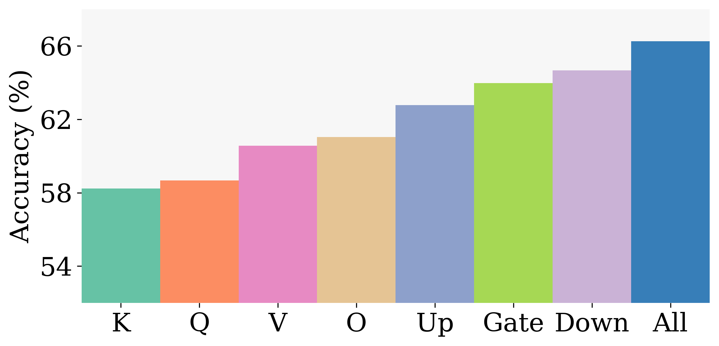
(a) GSM8K

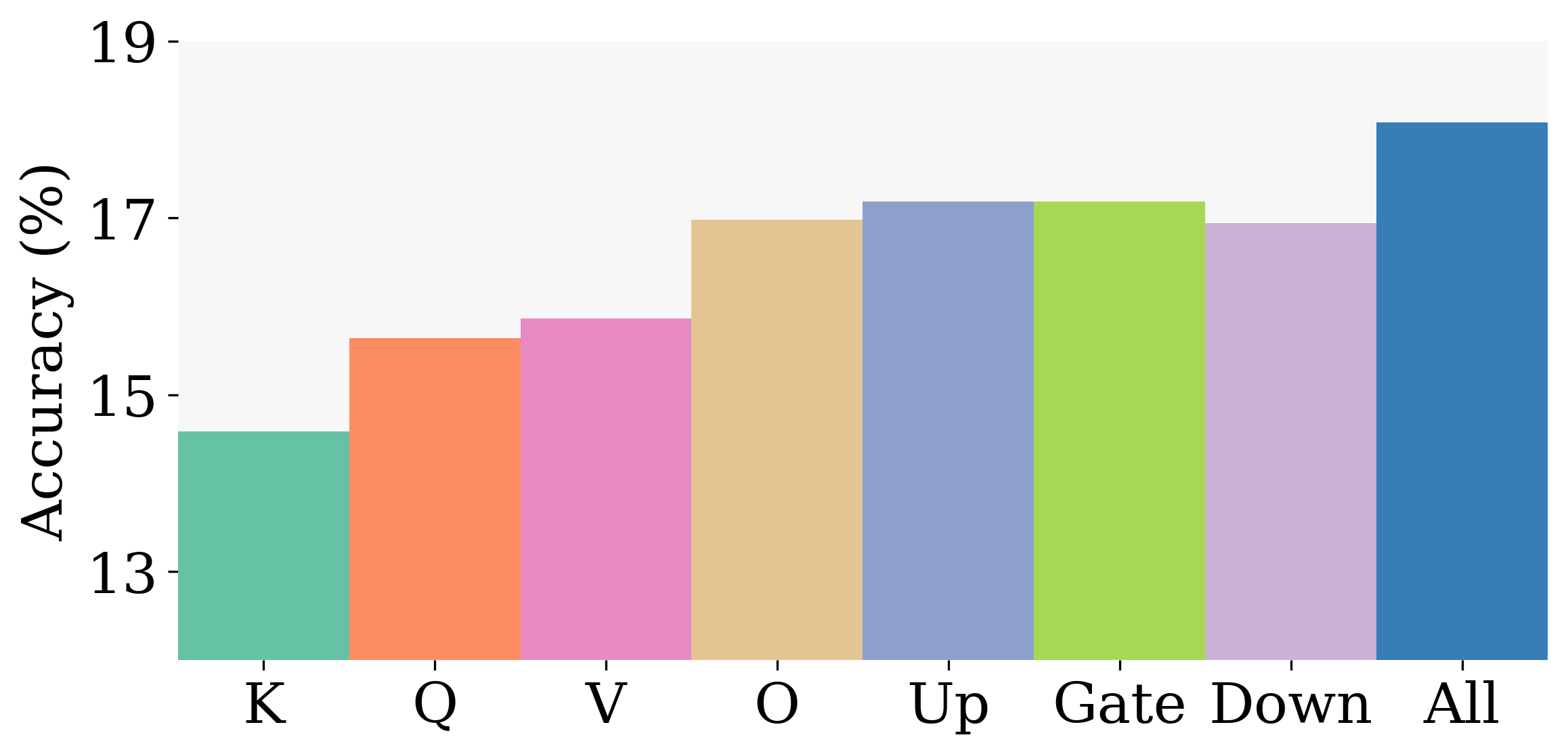
(b) MATH

Figure 3: Impact of selectively fine-tuning individual transformer components - Key, Query, Value, Output, Up, Gate, and Down projections, with ABBA (Mistral-7B).

4.4 All About Efficiency

Training Memory Footprint.

We report peak memory usage for various methods in Figure 4, measured with a batch size of $1$ and a context length of $256$. ABBA reduces memory consumption by $\approx 3-3.5$ times compared to full FT. Compared to other PEFT methods, ABBA offers similar memory efficiency to LoRA, and is $\approx 30-35\%$ more efficient than the next-best method, HiRA.

Training Time.

We benchmark training time across multiple settings in Table 9 (Appendix G). ABBA has comparable training time to LoRA, with only a $\approx 2-3\%$ overhead, primarily due to the additional computation introduced by the Hadamard product. We clarify that the initialization itself is highly efficient, as we compute the truncated SVD using torch.svd_lowrank. This computation takes less than one second for the entire model, even for the largest LLMs used in our experiments.

Efficient Inference.

At deployment time, ABBA supports efficient inference by pre-computing the update and merging it into the base weights as $W^{\prime}=W_{0}+(B_{1}A_{1})\odot(B_{2}A_{2})$. This allows models to switch tasks quickly by subtracting the update to restore $W_{0}$, then applying a new ABBA adapter. Since the update is fused ahead of inference, this incurs no runtime overhead or latency.

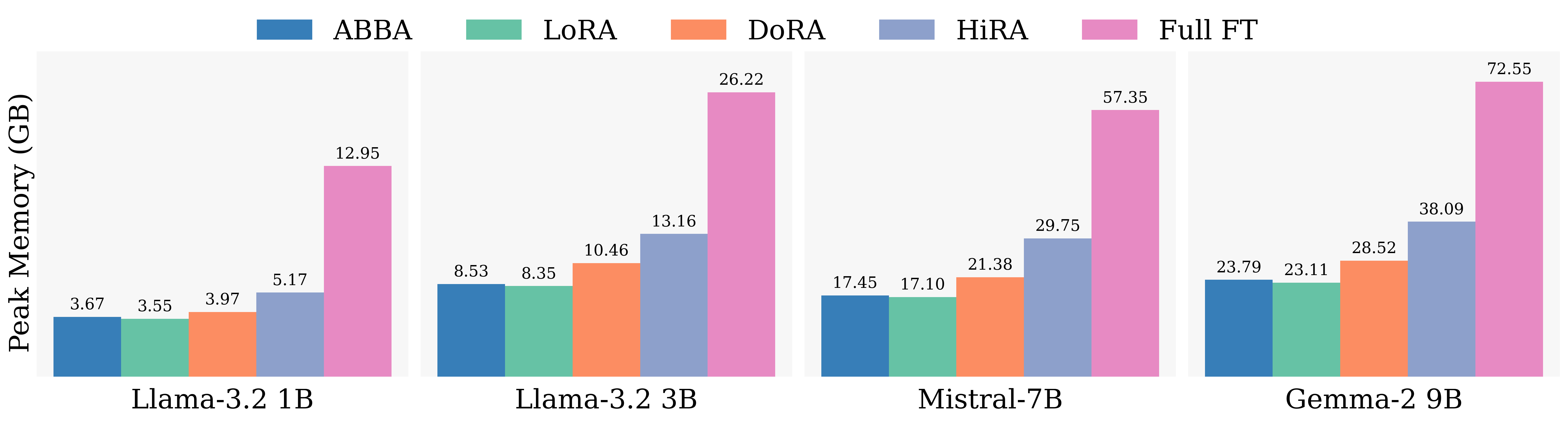
Figure 4: Comparison of training memory requirements across various methods. Results are reported for all models used in our work, with sequence length and batch size fixed at 256 and 1, respectively.

4.5 Extending ABBA via Adapter Chains

Table 6: Standard ABBA (2 pairs) versus a chained extension using 4 pairs.

Configuration	GSM8K	MATH
ABBA (2 pairs)	66.26	18.08
Chained ABBA (4 pairs)	64.84	17.74

A natural extension of ABBA is decomposing the update into a composition of $k$ multiple adapter pairs: $\Delta W=B_{1}A_{1}\odot B_{2}A_{2}\dots\odot B_{k}A_{k},$ where each adapter pair has rank $r/k$, with $r$ denoting the total rank budget. This factorized form increases the expressive capacity and the effective rank of the update. However, this introduces additional optimization challenges and may reduce training stability. We evaluate a variant of ABBA using a chain of four adapter pairs and compare it to the standard two-pair setup. As shown in Table 6, the chained version performs slightly worse, likely due to suboptimal scaling or training instability. We leave further investigation of multi-stage compositions to future work.

5 Conclusion

ABBA introduces a simple yet effective extension to the PEFT framework by expressing the weight update as a Hadamard product of two independently learnable low-rank matrices. This formulation retains the parameter efficiency of LoRA-style methods while enabling significantly higher expressivity. Our empirical results demonstrate that this expressivity translates to consistent performance gains across a range of tasks and models. Through a mathematically exact Khatri–Rao reformulation, ABBA matches LoRA’s efficiency while representing high-rank updates entirely through low-rank components, offering a more powerful and efficient alternative to existing PEFT approaches.

6 Limitations

Although we do not evaluate ABBA on ViTs or VLMs, our method is architecture-agnostic and should extend well to such models; we leave this to future work. While ABBA adapters can be merged into the base model to enable zero-overhead inference, serving many adapters concurrently may introduce additional compute due to the Hadamard structure. Lastly, we do not investigate the effect of merging multiple ABBA adapters within a single model. In LoRA, such composition can lead to destructive interference; whether similar effects arise with ABBA remains an open question.

Appendix

subsection

Appendix A Related Work

Parameter-Efficient Fine-Tuning (PEFT) and Low-Rank Adaptation (LoRA).

PEFT methods adapt large pretrained models to downstream tasks by training a small number of additional parameters while keeping the base model frozen. Among these, LoRA [10] is widely adopted for its simplicity and effectiveness, modeling the update $\Delta W$ as a low-rank product $BA$, thereby reducing trainable parameters significantly. Several extensions enhance LoRA along different axes. QLoRA [38] and QA-LoRA [39] combines quantization with LoRA to reduce memory footprint; AdaLoRA [40] allocates rank budgets dynamically across layers. LoRA-XS [12] inserts a small trainable core between frozen adapters to improve compression, while LoRA-Pro [14] and LoRA-SB [15] optimize adapters to better approximate full fine-tuning gradients. Other variants modify structure or initialization. VeRA [41] reuses frozen adapters across layers with task-specific scaling vectors; DoRA [11] applies low-rank updates only to the direction of pretrained weights. PiSSA [26] initializes adapters using top singular vectors, while rsLoRA [19] proposes scale-aware initialization to improve stability. Despite all these differences, these methods share a core principle: they represent $\Delta W$ using a low-rank structure, enabling adaptation under tight compute and memory constraints. LoRA-based methods have also been applied in other domains, such as federated fine-tuning [42, 21, 43, 44].

Beyond Low-Rank: High-Rank and Structured Adaptation.

While low-rank PEFT methods offer strong efficiency–performance tradeoffs, they can underperform in tasks requiring high-rank updates. This limitation has driven recent efforts to move beyond purely low-rank parameterizations. HiRA [13] achieves high-rank updates by taking the Hadamard (elementwise) product of the pretrained matrix $W_{0}$ with a low-rank adapter $BA$, leveraging the fact that such a product can increase effective rank without increasing parameter count. MoRA [45] instead learns a full-rank update through input compression and activation decompression, while KronA [46] uses Kronecker products between adapters to boost representational capacity. ReLoRA [47] uses multiple low-rank updates to approximate a final higher-rank update. Other approaches explore elementwise structure for different purposes: FLoRA [42] modulates intermediate activations per task using Hadamard products, and PACE [48] injects multiplicative noise during adaptation. These trends reflect a broader shift toward structured, high-rank updates for improved expressivity.

Our proposed method, ABBA, follows this direction by learning two independent low-rank matrices whose Hadamard product forms the update, enabling high-rank adaptation with full learnability and minimal overhead.

Appendix B Why Does No Closed-Form Reconstruction Solution Exist for ABBA?

SVD admits a closed-form solution for low-rank approximation because both the Frobenius and spectral norms are unitarily invariant. This allows the objective:

$$\min_{\operatorname{rank}(X)\leq k}\|M-X\|_{F}$$

to decouple along singular directions, as guaranteed by the Eckart–Young–Mirsky theorem [16, 17].

In contrast, ABBA solves the problem:

$$\min_{B_{1},B_{2},A_{1},A_{2}}\left\|M-(B_{1}A_{1})\odot(B_{2}A_{2})\right\|_{F}^{2},\quad\text{subject to }\operatorname{rank}(B_{\ell}A_{\ell})\leq r,$$

which is a non-convex, quartic optimization problem in the latent factors. The Hadamard product breaks orthogonal invariance; unlike the SVD, the two low-rank matrices $B_{1}A_{1}$ and $B_{2}A_{2}$ cannot be simultaneously diagonalized, and singular directions no longer decouple.

Using Theorem 1, one could, in principle, apply an SVD-like decomposition to $B_{1}\odot_{r}B_{2}$ and $A_{1}^{\top}\odot_{r}A_{2}^{\top}$. However, the rows of these matrices lie on a Segre variety $\mathcal{S}_{r_{1},r_{2}}$, meaning they reside in a highly constrained non-linear manifold. In general, such constraints prevent the existence of an exact closed-form solution unless every row lies in a rank-one $\mathbb{R}^{r_{1}\times r_{2}}$ subspace.

As a result, no analogue of truncated SVD exists for this formulation, and optimization must proceed via iterative methods such as gradient descent.

Appendix C Why Does LoRA-Style Initialization of Both Adapter Pairs Fail?

A naive LoRA-style initialization, where $B_{1}$ and $B_{2}$ are initialized to zero while $A_{1}$ and $A_{2}$ follow Kaiming uniform initialization, results in training failure due to gradients becoming identically zero. To analyze this, we compute the gradients of the loss with respect to each adapter component and show that they are exactly zero under this initialization, ultimately preventing any learning.

Notice that, for some input, $x$, the output, $y$, is of the form

$$y =Wx+\Delta Wx$$

$$=Wx+s_{\text{ABBA}}\left((B_{1}A_{1})\odot(B_{2}A_{2})\right)x$$

$$\mathcal{L} =f(y)$$

To get the final closed form gradients, we compute the gradients element-wise. We can therefore have, for some matrix $Z\in\{A_{1},A_{2},B_{1},B_{2}\}$,

$$\frac{\partial\mathcal{L}}{\partial Z_{pq}} =\sum_{i,j}\frac{\partial\mathcal{L}}{\partial\Delta W_{ij}}\frac{\partial\Delta W_{ij}}{\partial Z_{pq}}$$

$$=\sum_{i,j}\frac{\partial\mathcal{L}}{\partial\Delta W_{ij}}\frac{\partial\left(s_{\text{ABBA}}\left((B_{1}A_{1})\odot(B_{2}A_{2})\right)_{ij}\right)}{\partial Z_{pq}}$$

$$=s_{\text{ABBA}}\sum_{i,j}G_{ij}\cdot\frac{\partial\left((B_{1}A_{1})\odot(B_{2}A_{2})\right)_{ij}}{\partial Z_{pq}}$$ (8)

For $Z=A_{1}$.

We need to compute

$$\frac{\partial\mathcal{L}}{\partial A_{1,pq}} =s_{\text{ABBA}}\sum_{i,j}G_{ij}\cdot\frac{\partial\left((B_{1}A_{1})\odot(B_{2}A_{2})\right)_{ij}}{\partial A_{1,pq}}$$

$$=s_{\text{ABBA}}\sum_{i,j}G_{ij}\cdot\frac{\partial\left((B_{1}A_{1})_{ij}(B_{2}A_{2})_{ij}\right)}{\partial A_{1,pq}}$$

$$=s_{\text{ABBA}}\sum_{i,j}G_{ij}(B_{2}A_{2})_{ij}\frac{\partial\left((B_{1}A_{1})_{ij}\right)}{\partial A_{1,pq}}$$

$$=s_{\text{ABBA}}\sum_{i,j}G_{ij}(B_{2}A_{2})_{ij}\left(\sum_{l}\frac{\partial\left(B_{1,il}A_{1,lj}\right)}{\partial A_{1,pq}}\right)$$

Notice that $\frac{\partial\left(B_{1,il}A_{1,lj}\right)}{\partial A_{1,pq}}=0$ when $l\neq p$ and $j\neq q$ else $=B_{1,ip}$. This means we can rewrite the above summation as

$$\frac{\partial\mathcal{L}}{\partial A_{1,pq}} =s_{\text{ABBA}}\sum_{i}G_{iq}(B_{2}A_{2})_{iq}B_{1,ip}$$

$$=s_{\text{ABBA}}\sum_{i}(G\odot(B_{2}A_{2}))_{iq}B_{1,ip}$$

Notice that the above equation is nothing but a inner product of the $p^{\text{th}}$ row of $B_{1}^{\top}$ and $q^{\text{th}}$ column of $(G\odot(B_{2}A_{2}))$. We can therefore write the following

$$\frac{\partial\mathcal{L}}{\partial A_{1}} =s_{\text{ABBA}}B_{1}^{\top}(G\odot(B_{2}A_{2}))$$ (9)

For $Z=B_{1}$.

Following the same analysis as we did for $A_{1}$, we have the following for $B_{1}$.

$$\frac{\partial\mathcal{L}}{\partial B_{1,pq}} =s_{\text{ABBA}}\sum_{i,j}G_{ij}(B_{2}A_{2})_{ij}\left(\sum_{l}\frac{\partial\left(B_{1,il}A_{1,lj}\right)}{\partial B_{1,pq}}\right)$$

Again notice that $\frac{\partial\left(B_{1,il}A_{1,lj}\right)}{\partial B_{1,pq}}=0$ when $i\neq p$ and $l\neq q$ else $=A_{1,qj}$. This means we can rewrite the above summation as

$$\frac{\partial\mathcal{L}}{\partial B_{1,pq}} =s_{\text{ABBA}}\sum_{j}G_{pj}(B_{2}A_{2})_{pj}A_{1,qj}$$

$$=s_{\text{ABBA}}\sum_{j}(G\odot(B_{2}A_{2}))_{pj}A_{1,qj}$$

Notice that the above equation is nothing but a inner product of the $p^{\text{th}}$ row of $(G\odot(B_{2}A_{2}))$ and $q^{\text{th}}$ column of $A_{1}^{\top}$. We can therefore write the following

$$\frac{\partial\mathcal{L}}{\partial B_{1}} =s_{\text{ABBA}}(G\odot(B_{2}A_{2}))A_{1}^{\top}$$ (10)

It is also easy to see that our formulation is symmetric in $A_{i}$’s and $B_{i}$’s implying we also have

For $Z=B_{2}$.

Following Eqn. (10)

$$\frac{\partial\mathcal{L}}{\partial B_{2}} =s_{\text{ABBA}}(G\odot(B_{1}A_{1}))A_{2}^{\top}$$ (11)

For $Z=A_{2}$.

Following Eqn. (9),

$$\frac{\partial\mathcal{L}}{\partial A_{2}} =s_{\text{ABBA}}B_{2}^{\top}(G\odot(B_{1}A_{1}))$$ (12)

It is clear that initializing both $B_{1}$ and $B_{2}$ to zero causes all gradients to become zero, thereby preventing any learning and leading to complete training failure.

Appendix D Proofs

In this section, we provide the proofs for the assertions from the main text.

D.1 Proof of Theorem 1: Khatri–Rao Factorization

Proof.

We prove the equality by comparing the $(i,j)$-th elements of the left-hand side (LHS) and the right-hand side (RHS). Starting with the LHS, we have:

$$[(B_{1}A_{1})\odot(B_{2}A_{2})]_{ij} =(B_{1}A_{1})_{ij}\cdot(B_{2}A_{2})_{ij}$$

$$=\left(\sum_{k=1}^{r_{1}}B_{1,ik}A_{1,kj}\right)\cdot\left(\sum_{l=1}^{r_{2}}B_{2,il}A_{2,lj}\right)$$

$$=\sum_{k=1}^{r_{1}}\sum_{l=1}^{r_{2}}B_{1,ik}A_{1,kj}B_{2,il}A_{2,lj}.$$

Next, we analyze the RHS. Observe that $(B_{1}\odot_{r}B_{2})$ is an $m\times(r_{1}r_{2})$ matrix, and $(A_{1}^{\top}\odot_{r}A_{2}^{\top})$ is an $n\times(r_{1}r_{2})$ matrix. The matrix product on the RHS is:

$$\left[(B_{1}\odot_{r}B_{2})(A_{1}^{\top}\odot_{r}A_{2}^{\top})^{\top}\right]_{ij} =\sum_{f=1}^{r_{1}r_{2}}\left[B_{1}\odot_{r}B_{2}\right]_{if}\cdot\left[A_{1}^{\top}\odot_{r}A_{2}^{\top}\right]_{jf}.$$

To evaluate this sum, we define indices $k:=\left\lfloor\frac{f-1}{r_{2}}\right\rfloor+1$ and $l:=(f-1)\bmod r_{2}+1$, so that $f$ ranges over all $(k,l)$ pairs with $k\in[1,r_{1}]$ and $l\in[1,r_{2}]$. Then:

$$\left[B_{1}\odot_{r}B_{2}\right]_{if} =B_{1,ik}B_{2,il},$$

$$\left[A_{1}^{\top}\odot_{r}A_{2}^{\top}\right]_{jf} =A_{1,kj}A_{2,lj}.$$

Substituting back into the sum:

$$\sum_{f=1}^{r_{1}r_{2}}\left[B_{1}\odot_{r}B_{2}\right]_{if}\cdot\left[A_{1}^{\top}\odot_{r}A_{2}^{\top}\right]_{jf} =\sum_{k=1}^{r_{1}}\sum_{l=1}^{r_{2}}B_{1,ik}B_{2,il}A_{1,kj}A_{2,lj}.$$

This expression matches exactly with the earlier expansion of the LHS. Hence, the two sides are equal, completing the proof. ∎

Given two matrices $U,V\in\mathbb{R}^{m\times n}$, we define the row-wise Hadamard product, denoted by $U\odot_{r}V$. Let $U_{i}$ and $V_{i}$ denote the $i$-th rows of $U$ and $V$, respectively. The row-wise Hadamard product is computed as:

$$[U\odot_{r}V]_{i}:=[U_{i1}\cdot V_{i},\,U_{i2}\cdot V_{i},\,\dots,\,U_{in}\cdot V_{i}],$$

where each element of row $U_{i}$ scales the entire corresponding row $V_{i}$.

Consider the following example:

$$U=\begin{bmatrix}1&2\\ 3&4\end{bmatrix},\quad V=\begin{bmatrix}3&4\\ 5&6\end{bmatrix}.$$

Applying the row-wise Hadamard product $U\odot_{r}V$, we compute:

$$[U\odot_{r}V]_{1} :=[1\cdot V_{1},\;2\cdot V_{1}]=\begin{bmatrix}3&4&6&8\end{bmatrix},$$

$$[U\odot_{r}V]_{2} :=[3\cdot V_{2},\;4\cdot V_{2}]=\begin{bmatrix}15&18&20&24\end{bmatrix}.$$

Combining both rows, we obtain the final result:

$$U\odot_{r}V =\begin{bmatrix}3&4&6&8\\ 15&18&20&24\end{bmatrix}.$$

D.2 Proof of Theorem 2: Effective Scaling for ABBA Update

Proof.

We assume that each entry in the low-rank matrices $B_{i}$ and $A_{i}$ is independently drawn from a zero-mean distribution with variance $\sigma^{2}$. Therefore,

$$\mathbb{E}[B_{i,jk}^{2}]=\sigma^{2},\quad\mathbb{E}[A_{i,kj}^{2}]=\sigma^{2}.$$

We now compute the variance of a single element of the matrix product $B_{i}A_{i}$. For the first adapter pair:

$$\mathbb{E}\left[[B_{1}A_{1}]_{ij}^{2}\right] =\mathbb{E}\left[\left(\sum_{k=1}^{r_{1}}B_{1,ik}A_{1,kj}\right)^{2}\right]$$

$$=\sum_{k=1}^{r_{1}}\mathbb{E}[B_{1,ik}^{2}]\cdot\mathbb{E}[A_{1,kj}^{2}]$$

$$=r_{1}\sigma^{4}.$$

Similarly, for the second adapter pair:

$$\mathbb{E}\left[[B_{2}A_{2}]_{ij}^{2}\right]=r_{2}\sigma^{4}.$$

The ABBA update is defined as:

$$\Delta W_{ij}=s_{\text{ABBA}}\cdot(B_{1}A_{1}\odot B_{2}A_{2})_{ij},$$

and the variance of this update becomes:

$$\mathbb{E}[\Delta W_{ij}^{2}] =s_{\text{ABBA}}^{2}\cdot\mathbb{E}\left[(B_{1}A_{1})_{ij}^{2}\right]\cdot\mathbb{E}\left[(B_{2}A_{2})_{ij}^{2}\right]$$

$$=s_{\text{ABBA}}^{2}\cdot r_{1}r_{2}\cdot\sigma^{8}$$

$$=\left(s_{\text{ABBA}}\cdot\sqrt{r_{1}r_{2}}\cdot\sigma^{4}\right)^{2}.$$

To ensure stable training, we require this variance to match a desired target $\tau^{2}$. Assuming $\sigma=1$, this simplifies to:

$$\tau=s_{\text{ABBA}}\cdot\sqrt{r_{1}r_{2}}\quad\Rightarrow\quad s_{\text{ABBA}}=\frac{\tau}{\sqrt{r_{1}r_{2}}}.$$

Next, we determine the appropriate value of $\tau$ by aligning the effective scale of the ABBA update with that of two independently scaled LoRA-style adapters. LoRA typically applies a scaling factor of $\frac{\alpha_{\text{LoRA}}}{\sqrt{r}}$ to each low-rank adapter. Thus, composing two such adapters yields:

$$\left(\frac{\alpha_{\text{LoRA}}}{\sqrt{r_{1}}}B_{1}A_{1}\right)\odot\left(\frac{\alpha_{\text{LoRA}}}{\sqrt{r_{2}}}B_{2}A_{2}\right) =\frac{\alpha_{\text{LoRA}}^{2}}{\sqrt{r_{1}r_{2}}}(B_{1}A_{1}\odot B_{2}A_{2})$$

$$=\frac{\tau}{\sqrt{r_{1}r_{2}}}(B_{1}A_{1}\odot B_{2}A_{2}),$$

which implies $\tau=\alpha_{\text{LoRA}}^{2}$. Substituting this into the earlier expression for $s_{\text{ABBA}}$, we obtain:

$$s_{\text{ABBA}}=\frac{\alpha_{\text{LoRA}}^{2}}{\sqrt{r_{1}r_{2}}}.$$

This completes the proof. ∎

D.3 Proof of Theorem 3: Probabilistic Advantage of ABBA over LoRA

Definition 2 (Hadamard Product Manifold).

We define the Hadamard product manifold $\mathcal{M}_{\mathrm{Had}}\subset\mathbb{R}^{m\times n}$ as the set of all such matrices: $\mathcal{M}_{\mathrm{Had}}:=\left\{(B_{1}A_{1})\odot(B_{2}A_{2})\right\}\equiv\left\{(B_{1}\odot_{r}B_{2})(A_{1}\odot_{r}A_{2})\right\}.$

Proof.

Since $M_{\mathrm{true}}$ lies on the Hadamard manifold, we have $M_{\mathrm{ABBA},r}=M_{\mathrm{true}}$. Therefore, the reconstruction error using our ABBA formulation can be written as:

$$\|M-M_{\mathrm{ABBA},r}\|_{F}^{2}=\|M-M_{\mathrm{true}}\|_{F}^{2}=\|\sigma Z\|_{F}^{2}=\sigma^{2}\|Z\|_{F}^{2}.$$

Similarly, the reconstruction error for the SVD-based approximation is:

$$\|M-M_{\mathrm{SVD},r}\|_{F}^{2} =\|M_{\mathrm{true}}+\sigma Z-M_{\mathrm{SVD},r}\|_{F}^{2}$$

$$=\|M_{\mathrm{true}}-M_{\mathrm{SVD},r}\|_{F}^{2}+\sigma^{2}\|Z\|_{F}^{2}+2\sigma\langle Z,M_{\mathrm{true}}-M_{\mathrm{SVD},r}\rangle$$

$$=\epsilon_{\mathrm{bias}}^{2}+\sigma^{2}\|Z\|_{F}^{2}+2\sigma\langle Z,M_{\mathrm{true}}-M_{\mathrm{SVD},r}\rangle,$$

where we define $\epsilon_{\mathrm{bias}}^{2}:=\|M_{\mathrm{true}}-M_{\mathrm{SVD},r}\|_{F}^{2}$.

We now compute the difference between the two reconstruction errors:

$$\Delta :=\|M-M_{\mathrm{SVD},r}\|_{F}^{2}-\|M-M_{\mathrm{ABBA},r}\|_{F}^{2}$$

$$=\epsilon_{\mathrm{bias}}^{2}+2\sigma\langle Z,M_{\mathrm{true}}-M_{\mathrm{SVD},r}\rangle.$$

Since the entries of $Z$ are i.i.d. and distributed as $\mathcal{N}(0,1)$, the inner product $\langle Z,M_{\mathrm{true}}-M_{\mathrm{SVD},r}\rangle$ is normally distributed with mean $0$ and variance $\|M_{\mathrm{true}}-M_{\mathrm{SVD},r}\|_{F}^{2}=\epsilon_{\mathrm{bias}}^{2}$. Hence, $\Delta\sim\mathcal{N}\left(\epsilon_{\mathrm{bias}}^{2},4\sigma^{2}\epsilon_{\mathrm{bias}}^{2}\right)$.

We are interested in the probability that ABBA achieves a lower reconstruction error than SVD, i.e., $\mathbb{P}[\Delta>0]$. Applying the Chernoff tail bound:

$$\mathbb{P}[\Delta\leq 0]=\mathbb{P}\left[\langle Z,M_{\mathrm{true}}-M_{\mathrm{SVD},r}\rangle<-\frac{\epsilon_{\mathrm{bias}}^{2}}{2\sigma}\right]\leq\exp\left(-\frac{1}{2}\cdot\left(\frac{\epsilon_{\mathrm{bias}}^{2}}{2\sigma\cdot\sqrt{\epsilon_{\mathrm{bias}}^{2}}}\right)^{2}\right)$$

$$=\exp\left(-\frac{\epsilon_{\mathrm{bias}}^{2}}{8\sigma^{2}}\right)$$

$$\implies\mathbb{P}[\Delta>0]\geq 1-\delta$$

thus completing the proof. ∎

D.4 Proof of Theorem 4: Rank-Stability of ABBA Initialization

Proof.

We follow a similar analysis to that presented in LoRA-GA [49].

Forward $\text{2}^{\text{nd}}$ moment (ABBA adapter).

For any input $x\in\mathbb{R}^{d_{\text{in}}}$ with i.i.d. entries, the output of the ABBA adapter is given by:

$$y_{i}=s_{\text{ABBA}}\sum_{j=1}^{d_{\text{in}}}M_{1,ij}M_{2,ij}\cdot x_{j}\quad\forall i\in\{1,2,\ldots,d_{\text{out}}\}.$$ (14)

The second moment can then be expressed as:

$$\mathbb{E}[y_{i}^{2}]=s_{\text{ABBA}}^{2}\cdot\mathbb{E}\left[\left(\sum_{j=1}^{d_{\text{in}}}M_{1,ij}M_{2,ij}x_{j}\right)^{2}\right].$$

Gradient computation.

We next compute the gradients with respect to the input:

$$(\nabla_{x})_{j} =\sum_{i=1}^{d_{\text{out}}}\frac{\partial L}{\partial y_{i}}\frac{\partial y_{i}}{\partial x_{j}}=\sum_{i=1}^{d_{\text{out}}}\frac{\partial y_{i}}{\partial x_{j}}\cdot(\nabla)_{y_{i}}.$$

From Equation (14), we have:

$$\frac{\partial y_{i}}{\partial x_{j}}=s_{\text{ABBA}}\cdot M_{1,ij}M_{2,ij}.$$

Substituting, we obtain:

$$(\nabla_{x})_{j}=s_{\text{ABBA}}\sum_{i=1}^{d_{\text{out}}}M_{1,ij}M_{2,ij}\cdot(\nabla)_{y_{i}}.$$

Backward $\text{2}^{\text{nd}}$ moment.

We now compute the second moment of the gradient:

$$\mathbb{E}[(\nabla_{x})_{j}^{2}]=s_{\text{ABBA}}^{2}\cdot\mathbb{E}\left[\left(\sum_{i=1}^{d_{\text{out}}}M_{1,ij}M_{2,ij}\cdot(\nabla_{y})_{i}\right)^{2}\right].$$

Given our initialization, the entries of $M_{1}$ and $M_{2}$ are i.i.d., and thus:

$$\mathbb{E}[y_{i}^{2}] =s_{\text{ABBA}}^{2}\cdot\sum_{j=1}^{d_{\text{in}}}\mathbb{E}[M_{1,ij}^{2}]\cdot\mathbb{E}[M_{2,ij}^{2}]\cdot\mathbb{E}[x_{j}^{2}].$$

To compute $\mathbb{E}[M_{1,ij}^{2}]$ and $\mathbb{E}[M_{2,ij}^{2}]$, we use the fact that the entries of $A_{i}$ and $B_{i}$ are i.i.d., yielding:

$$\mathbb{E}[M_{l,ij}^{2}]=\sum_{k=1}^{r_{l}}\mathbb{E}[B_{l,ik}^{2}]\cdot\mathbb{E}[A_{l,kj}^{2}]=r_{l}\cdot\mathbb{E}[B_{l,11}^{2}]\cdot\mathbb{E}[A_{l,11}^{2}].$$

Combining terms, we obtain:

$$\mathbb{E}[y_{i}^{2}] =s_{\text{ABBA}}^{2}\cdot d_{\text{in}}\cdot r_{1}r_{2}\cdot\mathbb{E}[B_{1,11}^{2}]\cdot\mathbb{E}[A_{1,11}^{2}]\cdot\mathbb{E}[B_{2,11}^{2}]\cdot\mathbb{E}[A_{2,11}^{2}]\cdot\mathbb{E}[x_{j}^{2}],$$

$$\mathbb{E}[(\nabla_{x})_{j}^{2}] =s_{\text{ABBA}}^{2}\cdot d_{\text{out}}\cdot r_{1}r_{2}\cdot\mathbb{E}[B_{1,11}^{2}]\cdot\mathbb{E}[A_{1,11}^{2}]\cdot\mathbb{E}[B_{2,11}^{2}]\cdot\mathbb{E}[A_{2,11}^{2}]\cdot\mathbb{E}[(\nabla_{y})_{i}^{2}].$$

Stability under initialization.

To simplify our analysis, we assume that instead of setting $B_{1}=\mathbf{0}$, its entries are drawn i.i.d. from a distribution $\mathcal{D}$ with variance $\sigma_{B_{1}}^{2}$. Given that $s_{\text{ABBA}}\propto\frac{1}{\sqrt{r_{1}r_{2}}}$, we find:

Forward $\text{2}^{\text{nd}}$ moment:

Assuming $\mathbb{E}[x_{j}^{2}]=\Theta_{r_{1},r_{2}}(1)$, we have:

$$\mathbb{E}[y_{i}^{2}]=\mathcal{O}_{r_{1},r_{2}}(1)\cdot\sigma_{B_{1}}^{2}.$$

Backward $\text{2}^{\text{nd}}$ moment:

Assuming $\mathbb{E}[(\nabla_{y})_{i}^{2}]=\Theta_{r_{1},r_{2}}(1)$, we similarly obtain:

$$\mathbb{E}[(\nabla_{x})_{j}^{2}]=\mathcal{O}_{r_{1},r_{2}}(1)\cdot\sigma_{B_{1}}^{2}.$$

Conclusion.

Following Definition 1, these results imply that ABBA adapters are rank-stabilized. Moreover, even in the original case where $B_{1}=\mathbf{0}$, we observe that as $\sigma_{B_{1}}\to 0$, both variances converge to $\Theta_{r_{1},r_{2}}(0)$, still satisfying the criteria for rank stability. Therefore, we conclude that ABBA adapters remain rank-stabilized under the given initialization and scaling. ∎

Appendix E Selecting $\alpha$

In Theorem 2, we established the scaling relationship between ABBA and LoRA by comparing their respective factors, $\alpha_{\text{ABBA}}$ and $\alpha_{\text{LoRA}}$. To validate this empirically, we perform a sweep over different $\alpha_{\text{LoRA}}$ values and compute the corresponding ABBA scaling factors using $s_{\text{ABBA}}=\alpha_{\text{LoRA}}^{2}/\sqrt{r_{1}r_{2}}$, reporting results for Mistral-7B in Table 7. In line with our theoretical analysis and prior results in Table 4, ABBA performs best when $\alpha_{\text{LoRA}}$ lies in the typical range of 16–32.

Table 7: Performance comparison across different scaling factor values $s_{\text{ABBA}}$ for Mistral-7B.

$\mathbf{s_{\textbf{ABBA}}}$ ($\mathbf{\alpha_{\textbf{LoRA}}}$)	Accuracy ($\uparrow$)
	GSM8K	MATH
$1$ ($4$)	$62.17$	$17.10$
$4$ ($8$)	$64.06$	$17.60$
$8$ ($8\sqrt{2}$)	$64.43$	$18.14$
$16$ ($16$)	$66.10$	$18.16$
$32$ ($16\sqrt{2}$)	$66.26$	$18.08$
$64$ ($32$)	$65.81$	$17.68$
$128$ ($32\sqrt{2}$)	$65.20$	$16.82$
$256$ ($64$)	$64.79$	$15.08$

Appendix F Varying Rank

We evaluate ABBA on Mistral-7B while varying the total rank budget $r$, with $r_{1}=r_{2}=r/2$ and results shown in Table 8. Performance improves substantially from $r=16$ to $r=32$, with the best results achieved at $r=32$, after which gains begin to saturate. This aligns with our hypothesis: at $r=32$, ABBA’s effective rank reaches $r_{1}\times r_{2}=16\times 16=256$, which is significantly higher than the effective rank of 64 at $r=16$. The increased expressivity enables ABBA to better capture task-specific patterns. However, increasing the rank beyond $32$, or an effective rank beyond $256$, yields diminishing returns and may lead to overfitting, mirroring trends observed in using very high-ranked LoRA as well.

Table 8: Performance comparison of ABBA on Mistral-7B across varying total rank values $r$.

Rank	Accuracy ($\uparrow$)
	GSM8K	MATH
$16$	$64.97$	$18.06$
$32$	$\mathbf{66.26}$	$\mathbf{18.08}$
$64$	$65.05$	$17.98$
$128$	$65.73$	$17.96$

Appendix G Training Time

Following the discussion in Section 4.4, we report training times across all models and tasks in Table 9. ABBA incurs only a negligible overhead of approximately $2-3\%$ compared to LoRA, primarily due to the extra computation resulting from the Hadamard product.

Table 9: Training time comparison between ABBA and LoRA across multiple model and task settings.

Model	Training Time
	LoRA	ABBA
Llama-3.2 1B (Commonsense)	2:42:17	2:46:18
Llama-3.2 3B (Commonsense)	6:05:43	6:11:26
Mistral-7B (Arithmetic)	1:15:55	1:18:22
Gemma-2 9B (Arithmetic)	1:45:33	1:49:45

Appendix H Experimental Details

We implement all models using PyTorch [50] and HuggingFace Transformers [51]. All experiments run on a single NVIDIA A6000 GPU (48 GB). To reduce memory usage, we initialize base models in torch.bfloat16 precision. We train each configuration with the AdamW optimizer [52] and report the mean performance over three random seeds.

We configure Llama-3.2 1B, Llama-3.2 3B, Mistral-7B, and Gemma-2 9B using the hyperparameters shown in Table 10. We conduct a sweep over learning rates and scaling factors to identify optimal settings for each model-task pair. ABBA generally performs better with slightly higher learning rates compared to LoRA, and we recommend initiating hyperparameter sweeps in that range.

While we adopt most settings from prior work [27], we perform a targeted learning rate sweep to optimize performance. For baseline comparisons, we replicate the experimental setups from the original PiSSA [26], rsLoRA [19], DoRA [11], LoRA-Pro [14], and HiRA [13] papers to ensure fair and consistent evaluation.

Table 10: Hyperparameter settings for training Llama-3.2 1B and 3B on Commonsense170K, and Mistral-7B and Gemma-2 9B on MetaMathQA.

	Llama-3.2 1B / 3B	Mistral-7B / Gemma-2 9B
Optimizer	AdamW	AdamW
Batch size	$6$	$1$
Max. Seq. Len	$256$	$512$
Grad Acc. Steps	$24$	$32$
Epochs	$2$	$1$
Dropout	$0.05$	$0$
Learning Rate	$1\times 10^{-3}$	$1\times 10^{-3}$
LR Scheduler	Linear	Cosine
Warmup Ratio	$0.02$	$0.02$

Appendix I Dataset Details

CommonSense170K is a unified benchmark that aggregates eight commonsense reasoning datasets into a single multi-task setting [27]. Each instance is a multiple-choice question, and models are prompted to select the correct answer without providing explanations. We adopt the prompt format introduced by the paper [27]. Below, we briefly describe the constituent datasets:

• OBQA [28]: Open-book QA requiring retrieval and multi-hop reasoning over external knowledge.

• ARC Challenge (ARC-c) [29]: Difficult grade-school science questions designed to test advanced reasoning beyond surface heuristics.

• ARC Easy (ARC-e) [29]: Simpler science questions assessing core factual and conceptual understanding.

• WinoGrande [30]: Pronoun resolution tasks requiring commonsense inference to resolve ambiguity.

• HellaSwag [31]: Next-sentence prediction under a constrained completion setting, testing grounded understanding of everyday scenarios.

• PIQA [32]: Physical reasoning tasks where models select the most sensible solution to a practical problem.

• SIQA [33]: Social reasoning benchmark involving questions about intent, social dynamics, and consequences of human actions.

• BoolQ [34]: Binary (yes/no) questions drawn from natural queries, requiring contextual understanding of short passages.

MetaMathQA [35] reformulates existing mathematical problems into alternative phrasings that preserve their original semantics, offering diverse surface forms without introducing new information. We evaluate models fine-tuned on this dataset using two benchmarks: GSM8K [36], which targets step-by-step reasoning in elementary arithmetic word problems, and MATH [37], which features high-difficulty problems drawn from math competitions. We evaluate solely based on the correctness of the final numeric answer.

References

- (1) Alec Radford, Jong Wook Kim, Chris Hallacy, Aditya Ramesh, Gabriel Goh, Sandhini Agarwal, Girish Sastry, Amanda Askell, Pamela Mishkin, Jack Clark, Gretchen Krueger, and Ilya Sutskever. Learning transferable visual models from natural language supervision. In International Conference on Machine Learning, 2021.
- (2) Alexander Kirillov, Eric Mintun, Nikhila Ravi, Hanzi Mao, Chloe Rolland, Laura Gustafson, Tete Xiao, Spencer Whitehead, Alexander C. Berg, Wan-Yen Lo, Piotr Dollár, and Ross B. Girshick. Segment anything. 2023 IEEE/CVF International Conference on Computer Vision (ICCV), pages 3992–4003, 2023.
- (3) Josh Achiam, Steven Adler, Sandhini Agarwal, Lama Ahmad, Ilge Akkaya, Florencia Leoni Aleman, Diogo Almeida, Janko Altenschmidt, Sam Altman, Shyamal Anadkat, et al. Gpt-4 technical report. arXiv preprint arXiv:2303.08774, 2023.
- (4) Hugo Touvron, Louis Martin, Kevin Stone, Peter Albert, Amjad Almahairi, Yasmine Babaei, Nikolay Bashlykov, Soumya Batra, Prajjwal Bhargava, Shruti Bhosale, et al. Llama 2: Open foundation and fine-tuned chat models. arXiv preprint arXiv:2307.09288, 2023.
- (5) Gemini Team, Rohan Anil, Sebastian Borgeaud, Yonghui Wu, Jean-Baptiste Alayrac, Jiahui Yu, Radu Soricut, Johan Schalkwyk, Andrew M Dai, Anja Hauth, et al. Gemini: a family of highly capable multimodal models. arXiv preprint arXiv:2312.11805, 2023.
- (6) An Yang, Baosong Yang, Beichen Zhang, Binyuan Hui, Bo Zheng, Bowen Yu, Chengyuan Li, Dayiheng Liu, Fei Huang, Haoran Wei, et al. Qwen2. 5 technical report. arXiv preprint arXiv:2412.15115, 2024.
- (7) Gemma Team, Aishwarya Kamath, Johan Ferret, Shreya Pathak, Nino Vieillard, Ramona Merhej, Sarah Perrin, Tatiana Matejovicova, Alexandre Ramé, Morgane Rivière, et al. Gemma 3 technical report. arXiv preprint arXiv:2503.19786, 2025.
- (8) Sébastien Bubeck, Varun Chandrasekaran, Ronen Eldan, Johannes Gehrke, Eric Horvitz, Ece Kamar, Peter Lee, Yin Tat Lee, Yuanzhi Li, Scott Lundberg, et al. Sparks of artificial general intelligence: Early experiments with gpt-4. arXiv preprint arXiv:2303.12712, 2023.
- (9) Yaru Hao, Haoyu Song, Li Dong, Shaohan Huang, Zewen Chi, Wenhui Wang, Shuming Ma, and Furu Wei. Language models are general-purpose interfaces. (arXiv:2206.06336), June 2022. arXiv:2206.06336 [cs].
- (10) Edward J. Hu, Yelong Shen, Phillip Wallis, Zeyuan Allen-Zhu, Yuanzhi Li, Shean Wang, Lu Wang, and Weizhu Chen. Lora: Low-rank adaptation of large language models. (arXiv:2106.09685), October 2021. arXiv:2106.09685 [cs].
- (11) Shih-Yang Liu, Chien-Yi Wang, Hongxu Yin, Pavlo Molchanov, Yu-Chiang Frank Wang, Kwang-Ting Cheng, and Min-Hung Chen. Dora: Weight-decomposed low-rank adaptation. (arXiv:2402.09353), July 2024. arXiv:2402.09353 [cs].
- (12) Klaudia Bałazy, Mohammadreza Banaei, Karl Aberer, and Jacek Tabor. Lora-xs: Low-rank adaptation with extremely small number of parameters. (arXiv:2405.17604), October 2024. arXiv:2405.17604 [cs].
- (13) Qiushi Huang, Tom Ko, Zhan Zhuang, Lilian Tang, and Yu Zhang. HiRA: Parameter-efficient hadamard high-rank adaptation for large language models. In The Thirteenth International Conference on Learning Representations, 2025.
- (14) Zhengbo Wang, Jian Liang, Ran He, Zilei Wang, and Tieniu Tan. Lora-pro: Are low-rank adapters properly optimized? (arXiv:2407.18242), October 2024. arXiv:2407.18242 [cs].
- (15) Kaustubh Ponkshe, Raghav Singhal, Eduard Gorbunov, Alexey Tumanov, Samuel Horvath, and Praneeth Vepakomma. Initialization using update approximation is a silver bullet for extremely efficient low-rank fine-tuning. arXiv preprint arXiv:2411.19557, 2024.
- (16) Carl Eckart and Gale Young. The approximation of one matrix by another of lower rank. Psychometrika, 1(3):211–218, 1936.
- (17) Leon Mirsky. Symmetric gauge functions and unitarily invariant norms. The quarterly journal of mathematics, 11(1):50–59, 1960.
- (18) V. I. Slyusar. New operations of matrices product for applications of radars. In Proceedings of the International Seminar/Workshop on Direct and Inverse Problems of Electromagnetic and Acoustic Wave Theory (DIPED-97), pages 73–74, Lviv, Ukraine. PDF.
- (19) Damjan Kalajdzievski. A rank stabilization scaling factor for fine-tuning with lora. (arXiv:2312.03732), November 2023. arXiv:2312.03732 [cs].
- (20) Martino Ciaperoni, Aristides Gionis, and Heikki Mannila. The hadamard decomposition problem. Data Mining and Knowledge Discovery, 38(4):2306–2347, 2024.
- (21) Hyeon-Woo Nam, Ye-Bin Moon, and Tae-Hyun Oh. Fedpara: Low-rank hadamard product for communication-efficient federated learning. In Proceedings of the International Conference on Learning Representations (ICLR), 2022.
- (22) Shaowen Wang, Linxi Yu, and Jian Li. Lora-ga: Low-rank adaptation with gradient approximation. Advances in Neural Information Processing Systems, 37:54905–54931, 2024.
- (23) Abhimanyu Dubey, Abhinav Jauhri, Abhinav Pandey, Abhishek Kadian, Ahmad Al-Dahle, Aiesha Letman, Akhil Mathur, Alan Schelten, Amy Yang, Angela Fan, et al. The llama 3 herd of models. arXiv preprint arXiv:2407.21783, 2024.
- (24) Albert Q. Jiang, Alexandre Sablayrolles, Arthur Mensch, Chris Bamford, Devendra Singh Chaplot, Diego de las Casas, Florian Bressand, Gianna Lengyel, Guillaume Lample, Lucile Saulnier, Lélio Renard Lavaud, Marie-Anne Lachaux, Pierre Stock, Teven Le Scao, Thibaut Lavril, Thomas Wang, Timothée Lacroix, and William El Sayed. Mistral 7b, 2023.
- (25) Gemma Team, Morgane Riviere, Shreya Pathak, Pier Giuseppe Sessa, Cassidy Hardin, Surya Bhupatiraju, Léonard Hussenot, Thomas Mesnard, Bobak Shahriari, Alexandre Ramé, et al. Gemma 2: Improving open language models at a practical size. arXiv preprint arXiv:2408.00118, 2024.
- (26) Fanxu Meng, Zhaohui Wang, and Muhan Zhang. Pissa: Principal singular values and singular vectors adaptation of large language models. (arXiv:2404.02948), May 2024. arXiv:2404.02948 [cs].
- (27) Zhiqiang Hu, Lei Wang, Yihuai Lan, Wanyu Xu, Ee-Peng Lim, Lidong Bing, Xing Xu, Soujanya Poria, and Roy Ka-Wei Lee. Llm-adapters: An adapter family for parameter-efficient fine-tuning of large language models, 2023.
- (28) Todor Mihaylov, Peter Clark, Tushar Khot, and Ashish Sabharwal. Can a suit of armor conduct electricity? a new dataset for open book question answering. arXiv preprint arXiv:1809.02789, 2018.
- (29) Peter Clark, Isaac Cowhey, Oren Etzioni, Tushar Khot, Ashish Sabharwal, Carissa Schoenick, and Oyvind Tafjord. Think you have solved question answering? try arc, the ai2 reasoning challenge. arXiv preprint arXiv:1803.05457, 2018.
- (30) Keisuke Sakaguchi, Ronan Le Bras, Chandra Bhagavatula, and Yejin Choi. Winogrande: An adversarial winograd schema challenge at scale. Communications of the ACM, 64(9):99–106, 2021.
- (31) Rowan Zellers, Ari Holtzman, Yonatan Bisk, Ali Farhadi, and Yejin Choi. Hellaswag: Can a machine really finish your sentence? arXiv preprint arXiv:1905.07830, 2019.
- (32) Yonatan Bisk, Rowan Zellers, Jianfeng Gao, Yejin Choi, et al. Piqa: Reasoning about physical commonsense in natural language. In Proceedings of the AAAI conference on artificial intelligence, volume 34, pages 7432–7439, 2020.
- (33) Maarten Sap, Hannah Rashkin, Derek Chen, Ronan LeBras, and Yejin Choi. Socialiqa: Commonsense reasoning about social interactions. arXiv preprint arXiv:1904.09728, 2019.
- (34) Christopher Clark, Kenton Lee, Ming-Wei Chang, Tom Kwiatkowski, Michael Collins, and Kristina Toutanova. Boolq: Exploring the surprising difficulty of natural yes/no questions. arXiv preprint arXiv:1905.10044, 2019.
- (35) Longhui Yu, Weisen Jiang, Han Shi, Jincheng Yu, Zhengying Liu, Yu Zhang, James T. Kwok, Zhenguo Li, Adrian Weller, and Weiyang Liu. Metamath: Bootstrap your own mathematical questions for large language models, 2024.
- (36) Karl Cobbe, Vineet Kosaraju, Mohammad Bavarian, Mark Chen, Heewoo Jun, Lukasz Kaiser, Matthias Plappert, Jerry Tworek, Jacob Hilton, Reiichiro Nakano, Christopher Hesse, and John Schulman. Training verifiers to solve math word problems, 2021.
- (37) Dan Hendrycks, Collin Burns, Saurav Kadavath, Akul Arora, Steven Basart, Eric Tang, Dawn Song, and Jacob Steinhardt. Measuring mathematical problem solving with the math dataset, 2021.
- (38) Tim Dettmers, Artidoro Pagnoni, Ari Holtzman, and Luke Zettlemoyer. Qlora: efficient finetuning of quantized llms. In Proceedings of the 37th International Conference on Neural Information Processing Systems, NIPS ’23, Red Hook, NY, USA, 2024. Curran Associates Inc.
- (39) Yuhui Xu, Lingxi Xie, Xiaotao Gu, Xin Chen, Heng Chang, Hengheng Zhang, Zhengsu Chen, Xiaopeng Zhang, and Qi Tian. Qa-lora: Quantization-aware low-rank adaptation of large language models. arXiv preprint arXiv:2309.14717, 2023.
- (40) Qingru Zhang, Minshuo Chen, Alexander Bukharin, Nikos Karampatziakis, Pengcheng He, Yu Cheng, Weizhu Chen, and Tuo Zhao. Adalora: Adaptive budget allocation for parameter-efficient fine-tuning, 2023.
- (41) Dawid J. Kopiczko, Tijmen Blankevoort, and Yuki M. Asano. Vera: Vector-based random matrix adaptation. (arXiv:2310.11454), January 2024. arXiv:2310.11454 [cs].
- (42) Ziyao Wang, Zheyu Shen, Yexiao He, Guoheng Sun, Hongyi Wang, Lingjuan Lyu, and Ang Li. Flora: Federated fine-tuning large language models with heterogeneous low-rank adaptations, 2024.
- (43) Raghav Singhal, Kaustubh Ponkshe, and Praneeth Vepakomma. Fedex-lora: Exact aggregation for federated and efficient fine-tuning of foundation models. arXiv preprint arXiv:2410.09432, 2025.
- (44) Raghav Singhal, Kaustubh Ponkshe, Rohit Vartak, Lav R Varshney, and Praneeth Vepakomma. Fed-sb: A silver bullet for extreme communication efficiency and performance in (private) federated lora fine-tuning. arXiv preprint arXiv:2502.15436, 2025.
- (45) Ting Jiang, Shaohan Huang, Shengyue Luo, Zihan Zhang, Haizhen Huang, Furu Wei, Weiwei Deng, Feng Sun, Qi Zhang, Deqing Wang, and Fuzhen Zhuang. Mora: High-rank updating for parameter-efficient fine-tuning, 2024.
- (46) Ali Edalati, Marzieh Tahaei, Ivan Kobyzev, Vahid Partovi Nia, James J Clark, and Mehdi Rezagholizadeh. Krona: Parameter efficient tuning with kronecker adapter. arXiv preprint arXiv:2212.10650, 2022.
- (47) Vladislav Lialin, Namrata Shivagunde, Sherin Muckatira, and Anna Rumshisky. Relora: High-rank training through low-rank updates. arXiv preprint arXiv:2307.05695, 2023.
- (48) Yao Ni, Shan Zhang, and Piotr Koniusz. Pace: Marrying generalization in parameter-efficient fine-tuning with consistency regularization, 2025.
- (49) Shaowen Wang, Linxi Yu, and Jian Li. Lora-ga: Low-rank adaptation with gradient approximation. (arXiv:2407.05000), July 2024. arXiv:2407.05000 [cs].
- (50) Adam Paszke, Sam Gross, Francisco Massa, Adam Lerer, James Bradbury, Gregory Chanan, Trevor Killeen, Zeming Lin, Natalia Gimelshein, Luca Antiga, et al. Pytorch: An imperative style, high-performance deep learning library. Advances in neural information processing systems, 32, 2019.
- (51) Thomas Wolf, Lysandre Debut, Victor Sanh, Julien Chaumond, Clement Delangue, Anthony Moi, Pierric Cistac, Tim Rault, Rémi Louf, Morgan Funtowicz, et al. Transformers: State-of-the-art natural language processing. In Proceedings of the 2020 conference on empirical methods in natural language processing: system demonstrations, pages 38–45, 2020.
- (52) Ilya Loshchilov and Frank Hutter. Decoupled weight decay regularization, 2019.