MSDformer: Multi-scale Discrete Transformer For Time Series Generation

Abstract

Discrete Token Modeling (DTM), which employs vector quantization techniques, has demonstrated remarkable success in modeling non-natural language modalities, particularly in time series generation. While our prior work SDformer established the first DTM-based framework to achieve state-of-the-art performance in this domain, two critical limitations persist in existing DTM approaches: 1) their inability to capture multi-scale temporal patterns inherent to complex time series data, and 2) the absence of theoretical foundations to guide model optimization. To address these challenges, we proposes a novel multi-scale DTM-based time series generation method, called Multi-Scale Discrete Transformer (MSDformer). MSDformer employs a multi-scale time series tokenizer to learn discrete token representations at multiple scales, which jointly characterize the complex nature of time series data. Subsequently, MSDformer applies a multi-scale autoregressive token modeling technique to capture the multi-scale patterns of time series within the discrete latent space. Theoretically, we validate the effectiveness of the DTM method and the rationality of MSDformer through the rate-distortion theorem. Comprehensive experiments demonstrate that MSDformer significantly outperforms state-of-the-art methods. Both theoretical analysis and experimental results demonstrate that incorporating multi-scale information and modeling multi-scale patterns can substantially enhance the quality of generated time series in DTM-based approaches. The code will be released upon acceptance.

I Introduction

Time series data is integral to numerous real-world applications, including finance [1, 2, 3, 4, 5], healthcare [6], energy [7, 8, 9, 10], retail [11, 12], and climate science [13]. Despite its importance, the scarcity of dynamic data often hinders the advancement of machine learning solutions, especially in contexts where data sharing might compromise privacy [14]. To address this challenge, the generation of synthetic yet realistic time series data has gained traction as a viable alternative. This approach has become increasingly popular, driven by recent progress in deep learning methodologies.

The deep learning revolution introduces three principal paradigms for temporal data synthesis: Generative Adversarial Networks (GANs) [15, 16, 17, 18, 19, 20, 21], which pioneer adversarial training frameworks that capture sharp temporal distributions but suffer from non-convex optimization instability and catastrophic mode collapse; Variational Autoencoders (VAEs) [22, 23], which ensure training stability via evidence lower bound optimization with KL-regularized latent spaces, at the expense of over-smoothed outputs that attenuate high-frequency details; Denoising Diffusion Probabilistic Models (DDPMs) [24, 25, 26], which achieve state-of-the-art performance through iterative denoising processes but face deployment challenges, including architectural complexity, limited controllability, and computational inefficiency.

In recent years, large transformer-based language models, commonly referred to as LMs or LLMs, have emerged as the predominant solution for natural language generation tasks [27, 28]. These models have demonstrated remarkable capabilities in generating high-quality text and have progressively expanded their applications to encompass various modalities beyond natural language. Notably, significant advancements have been made in image generation [29, 30, 31, 32], video synthesis [33, 34, 35], and audio generation [36, 37, 38] through the innovative application of Discrete Token Modeling (DTM) technique. DTM operates by learning discrete representations of diverse data modalities and treating them in a manner analogous to natural language tokens. This technique enables direct adaptation of pre-trained language models for cross-modal generation tasks. The success of these methods has been substantial, yielding impressive results in various multimodal generation tasks.

The remarkable success of the DTM technique in visual and audio domains has motivated its recent extension to time series tasks [39, 40]. Specifically, our prior work SDformer [39] established the first DTM-based framework that demonstrates statistically significant superiority over GANs, VAEs, and DDPMs in the time series generation task. Despite these empirical successes, the theoretical foundations of DTM remain underdeveloped, which limits its methodological advancement and broader application. Moreover, complex time series often exhibit multi-scale temporal patterns, encompassing both low-frequency trends and short-term fluctuations. Current DTM-based approaches for time series generation, such as SDformer, predominantly utilize single-scale modeling frameworks. This limitation restricts their ability to comprehensively capture the multi-scale temporal patterns inherent in complex time series data.

To address the aforementioned challenges, we propose a novel DTM-based framework for time series generation, termed the Multi-Scale Discrete Transformer (MSDformer). This framework extends SDformer [39], advancing from single-scale to multi-scale modeling. Similar to existing DTM-based approaches, MSDformer operates in a two-stage pipeline. In the first stage, MSDformer constructs a multi-scale time series tokenizer through cascaded residual VQ-VAEs [41, 42], progressively learning discrete token representations at multiple scales. These multi-scale token sequences collectively capture the comprehensive characteristics of the original time series, enabling a more nuanced representation of both low-frequency and high-frequency features. In the second stage, MSDformer adopts an autoregressive token modeling technique to learn the distribution of multi-scale token sequences, thereby effectively capturing the multi-scale temporal patterns inherent in time series data. This technique is naturally better suited to sequential data than the masked token modeling technique, as illustrated by SDformer. Furthermore, we prove that DTM-based methods offer superior controllability in the rate-distortion trade-off compared to other continuous models, leveraging Shannon’s Rate-Distortion Theorem. Based on this, we further theoretically demonstrate that multi-scale modeling can achieve lower distortion.

In summary, our contributions include:

• We introduce a novel DTM-based method, MSDformer, which extends SDformer by an advancement from single-scale to multi-scale modeling. This advancement enables MSDformer to effectively capture the multi-scale temporal patterns inherent in time series data, thereby enhancing generative capabilities.

• We theoretically demonstrate that DTM-based methods offer superior controllability in the rate-distortion trade-off compared to other continuous models, and that multi-scale modeling allows for lower distortion.

• Our experimental results confirm that the MSDformer’s performance in time series generation notably surpasses those of current methods, exemplified by an average enhancement of 34.5% in Discriminative Score and 12.6% in Context-FID Score to SDformer under long-term time series generation tasks.

II Related Work

In this section, we focus on two key directions: 1) advancements in time series generative models, and 2) the applications and developments of the discrete token modeling technique, both of which jointly motivate our framework.

II-A Time Series Generation

With the continuous advancement of deep generative models, the field of time series generation has achieved remarkable progress. The initial wave of research predominantly focuses on Generative Adversarial Networks (GANs) as the primary architecture for time series generation [15, 16, 17, 18, 19, 20]. For example, TimeGAN [17] introduces novel enhancements by incorporating an embedding function and supervised loss to better capture temporal dynamics. COT-GAN [18] innovatively combines the underlying principles of GANs with Causal Optimal Transfer theory, enabling stable generation of both low- and high-dimensional time series data. Despite these advancements, inherent challenges such as training instability and mode collapse persist, prompting researchers to explore alternative architectures.

The limitations of GAN-based approaches prompt researchers to turn to Variational Autoencoders (VAEs) for time series generation. For example, TimeVAE [22], with its interpretable temporal structure, stands out as a significant advancement, delivering superior performance in time series synthesis. KoVAE [23] integrates Koopman operator theory with VAEs to provide a unified modeling framework for both regular and irregular time series data. However, these methods often face the issue of generating samples that lack detail and diversity.

Denoising Diffusion Probabilistic Models (DDPMs) [43] mark a transformative phase in generative modeling, with rapid adaptation to time series generation. Early applications like DiffWave [24] demonstrate the potential of DDPMs in waveform generation, while more recent innovations such as DiffTime [25] leverages advanced score-based diffusion models for enhanced temporal data synthesis. The field reaches new heights with Diffusion-TS [26], a diffusion model framework that generates high-quality multivariate time series samples using an encoder-decoder Transformer architecture with disentangled temporal representations. While these methods exhibit superior generative capabilities, they are confronted with several challenges, including architectural complexity, limited controllability, and computational inefficiency.

II-B Discrete Token Modeling

Discrete Token Modeling (DTM) is a technique for modeling discrete token sequences using sequence models, originally widely applied in natural language modalities. In recent years, the rise of large-scale language models has driven a new era of development in artificial intelligence [27, 28], highlighting the efficiency of the DTM technique. Building on its success in natural language tasks, DTM has been extended to non-natural language modalities—such as vision, audio, and time series—through vector quantization models like VQ-VAE [42] and VQ-GAN [44].

Early DTM approaches in non-natural language modalities primarily rely on two paradigms: Autoregressive Token Modeling (ARTM) and Masked Token Modeling (MTM). ARTM predicts the next token in a sequence based on previous tokens using a categorical distribution. Notable examples include DALL-E [29] and Parti [30] for text-to-image generation, and T2M-GPT [45] and MotionGPT [46] for text-to-motion synthesis. In contrast, MTM employs a masked token prediction objective [47], reconstructing randomly masked tokens using the observed context. This approach has been adopted by models like MaskGIT [31] and MUSE [32] for image generation, and extended to video generation in MAGVIT [33] and Phenaki [34], demonstrating its versatility.

Recently, a novel DTM paradigm called Visual AutoRegressive Modeling (VAR)[48] has emerged. VAR redefines autoregressive modeling as coarse-to-fine ”next-scale prediction” or ”next-resolution prediction”. During tokenization, images are encoded into multi-scale token maps via hierarchical quantization. The generation process then proceeds autoregressively from low to high resolutions, with each step predicting the next higher-resolution token map. This multi-scale autoregressive approach enhances spatial coherence and preserves local details, resulting in higher-quality and more natural image synthesis.

Inspired by the broad applicability of the DTM technique across modalities, researchers have begun exploring its potential for time series tasks [39, 40]. HDT [40] proposes a hierarchical DTM-based framework that achieves high accuracy in high-dimensional, long-term time series forecasting tasks. Our prior work, SDformer [39], introduces the DTM technique to time series generation and proposes a similarity-driven vector quantization method, achieving a significant breakthrough in generation quality.

III Problem Statement

Consider a multivariate time series as a sequence of observations denoted by $x_{1:\tau}=(x_{1},\cdots,x_{\tau})\in\mathbb{R}^{\tau\times d}$, where $\tau$ represents the number of time steps and $d$ denotes the dimensionality of variables at each time step. In practical applications, we typically work with a collection of such time series. Formally, a dataset containing $n$ time series can be represented as $D=\{x_{1:\tau}^{i}\}_{i=1}^{n}$, where each $x_{1:\tau}^{i}$ corresponds to an independent realization of the underlying temporal process.

The task of time series generation aims to learn the intrinsic distribution of the observed dataset $D$ and subsequently generate new, realistic time series samples that preserve the statistical properties of the original dataset. Mathematically, this can be formulated as learning a generative model $f_{\theta}$ that maps samples from a known prior distribution to the time series domain:

$$\hat{x}_{1:\tau}^{i}=f_{\theta}(Z),$$ (1)

where $Z$ is typically sampled from a simple distribution (e.g., Gaussian distribution) and serves as the source of randomness for generation.

IV Methods

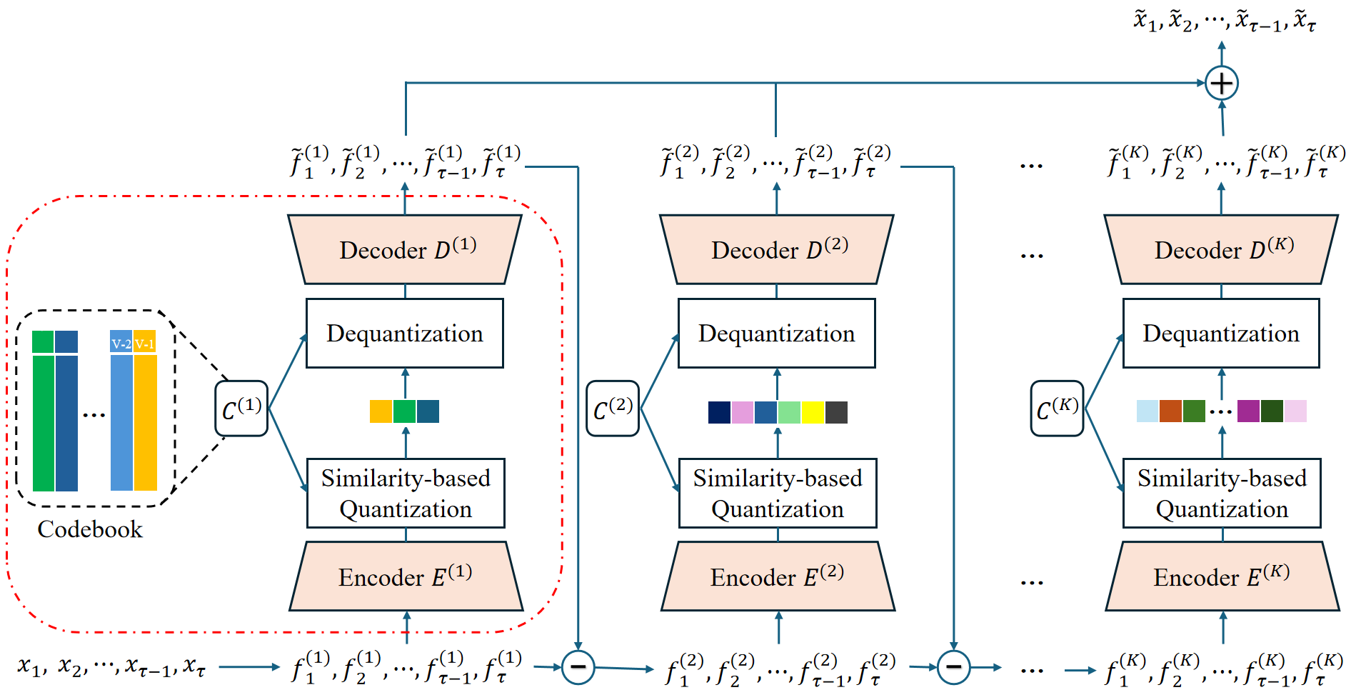
Figure 1: The workflow of multi-scale time series tokenizer. The multi-scale time series tokenizer comprises $K$ modules, each of which is a VQ-VAE model that employs a similarity-driven vector quantization method to learn discrete token representations at different scales. Specifically, the first scale is used to model the large-scale information of the time series, while each subsequent scale models the difference between the input and output of the previous scale. The discrete token sequences obtained at each scale are then combined to jointly characterize the complete time series data. Notably, when $K=1$, the model degenerates to SDformer’s single-scale time series tokenizer [39], as shown by the red dashed line in the figure.

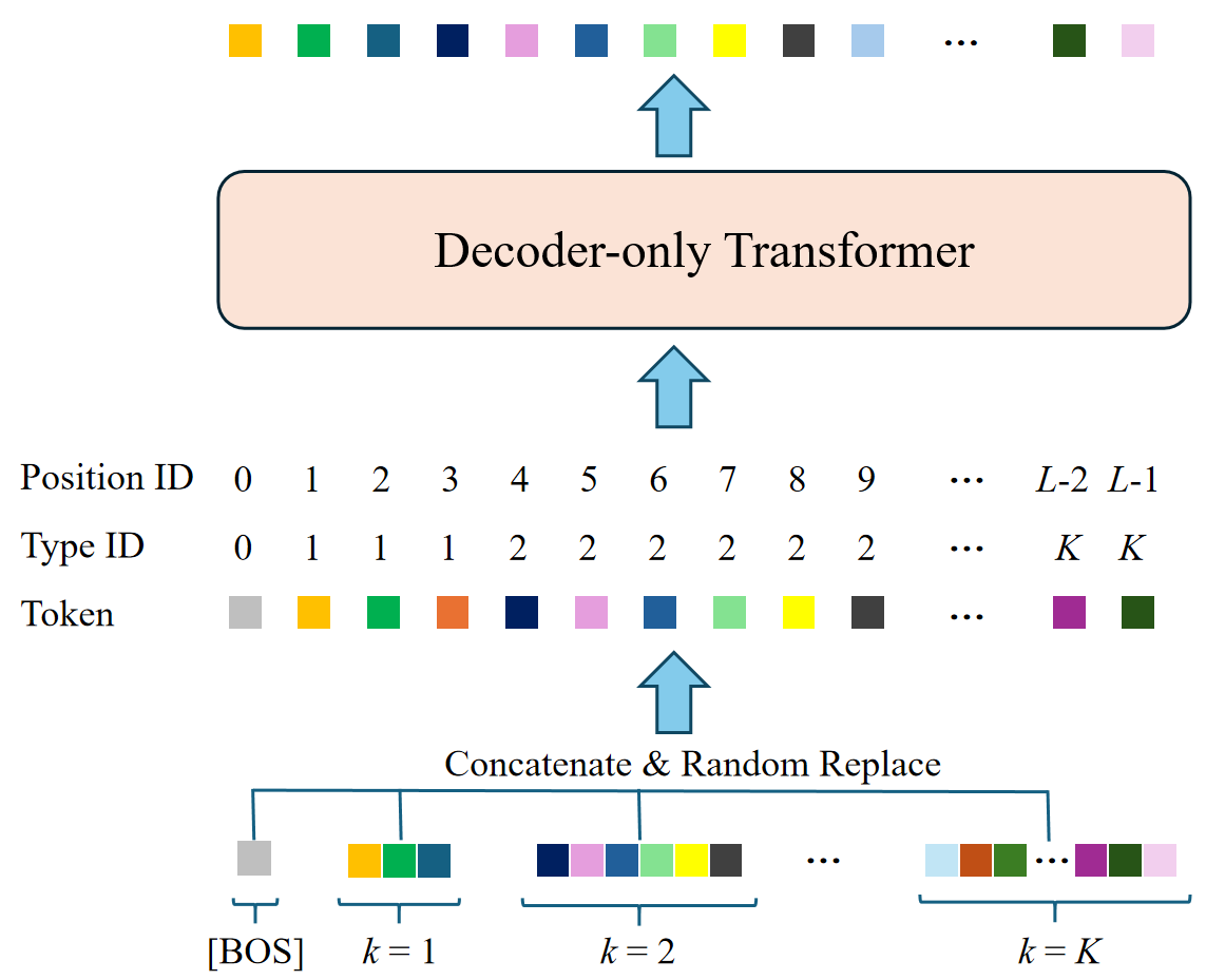
Figure 2: The workflow of the second stage of MSDformer: Multi-Scale Autoregressive Token Modeling. In this stage, the [BOS] token is first concatenated with the discrete token sequence of each scale. The resulting sequence, along with the token type ID and position ID, is then fed into the Decoder-only Transformer to predict the next token at each position. Notably, when $K=1$, the model degenerates to SDformer’s single-scale autoregressive token modeling [39].

In this section, we introduce MSDformer, a novel multi-scale DTM-based model tailored for time series generation. MSDformer is a two-stage framework designed to learn and model multi-scale information and patterns in time series data. In the first stage, MSDformer employs a multi-scale time series tokenizer that leverages similarity-driven vector quantization to generate high-quality discrete token representations across multiple scales, as depicted in Fig. 1. Building on these multi-scale discrete token representations, the second stage utilizes a multi-scale autoregressive token modeling technique to capture the multi-scale patterns of time series in the discrete latent space, as illustrated in Fig. 2.

IV-A Multi-scale Time Series Tokenizer

The multi-scale tokenizer implements cascaded residual learning [41] through stacked VQ-VAE models [42], where each subsequent model hierarchically encodes residual information from the preceding scale. This coarse-to-fine decomposition progressively refines temporal features, yielding more precise and detailed representations of the underlying time series data.

Let there be $K$ scales, each with an encoder $\mathcal{E}^{(k)}$, a decoder $\mathcal{D}^{(k)}$, a codebook $C^{(k)}$, and a downsampling factor $r^{(k)}$, where $k=1,\ldots,K$. The learnable codebook $C^{(k)}=\{c_{v}\}_{v=0}^{V^{(k)}-1}\subset\mathbb{R}^{d_{c}}$ at each scale contains $V^{(k)}$ latent embedding vectors, each of dimension $d_{c}$. The downsampling factor $r^{(k)}\geq 1$ decreases as $k$ increases, meaning that smaller $k$ processes larger scale information.

The input to the model at each scale is the residual $f_{1:\tau}^{(k)}\in\mathbb{R}^{\tau\times d}$. When $k=1$, $f_{1:\tau}^{(k)}$ is initialized as $x_{1:\tau}$. For $k>1$, $f_{1:\tau}^{(k)}$ is the residual between the input of the previous scale and its reconstruction output. Specifically, starting from $k=1$, the following operations are performed:

(1) Encoding Process. First, the encoder $\mathcal{E}^{(k)}$ initially applies 1D convolutions to the input $f_{1:\tau}^{(k)}$ along the temporal dimension, producing encoded vector:

$$h_{1:L^{(k)}}^{(k)}=\mathcal{E}^{(k)}(f_{1:\tau}^{(k)}),$$ (2)

where $h_{1:L^{(k)}}^{(k)}\in\mathbb{R}^{L^{(k)}\times d_{c}}$ is the encoded feature, and $L^{(k)}=\tau/r^{(k)}$ is the length in the discrete latent space at the $k$-th scale.

(2) Vector Quantization. Then, the similarity-driven vector quantization $Q(\ \cdot\ ;C^{(k)})$ identifies the index of the vector in the codebook $C^{(k)}$ that exhibits the highest similarity to $h_{i}^{(k)}$, which can be expressed as:

$$y_{i}^{(k)}=Q(h_{i}^{(k)};C^{(k)}):=\arg\max_{v}h_{i}^{(k)}\cdot c_{v}^{(k)},$$ (3)

where $\cdot$ denotes the inner product, and the discrete token sequence of the $k$-th scale can be represented as $y_{1:L^{(k)}}^{(k)}\in\prod_{\ell=1}^{L^{(k)}}\{0,1,\ldots,V^{(k)}-1\}$, with $\prod$ denoting the Cartesian product.

(3) Dequantization Process. Following quantization, the dequantization process $Q^{-1}(\ \cdot\ ;C^{(k)})$ reverts $y_{i}^{(k)}$ back to the latent embedding vector, denoted as:

$$\tilde{h}_{i}^{(k)}=Q^{-1}(y_{i}^{(k)};C^{(k)}):=c_{y_{i}^{(k)}}^{(k)},$$ (4)

(4) Decoding Process. Subsequently, the decoder $\mathcal{D}^{(k)}$ restores it to the raw time series space:

$$\tilde{f}_{1:\tau}^{(k)}=\mathcal{D}^{(k)}(\tilde{h}_{1:L^{(k)}}^{(k)}).$$ (5)

(5) Residual Calculation. Lastly, we obtain the residual input for the next scale, denoted as:

$$f_{1:\tau}^{(k+1)}=f_{1:\tau}^{(k)}-\tilde{f}_{1:\tau}^{(k)}.$$ (6)

After completing the above steps, continue to repeat the above operations of modeling the residual $f_{1:\tau}^{(k+1)}$ at the $(k+1)$-th scale until the $K$-th scale, following steps (1)-(5).

After processing all scales as described above, the final reconstruction of the time series is achieved by aggregating the reconstruction results from all scales:

$$\tilde{x}_{1:\tau}=\sum_{k=1}^{K}\tilde{f}_{1:\tau}^{(k)}.$$ (7)

To train this multi-scale time series tokenizer, we utilize two distinct loss functions for training and optimizing the parameters of $\mathcal{E}^{(k)}$ and $\mathcal{D}^{(k)}$:

$$\mathcal{L}=\left\|x_{1:\tau}-\tilde{x}_{1:\tau}\right\|_{2}^{2}+\lambda\sum_{k=1}^{K}\frac{1}{L^{(k)}}\sum_{i=1}^{L^{(k)}}\left(1-h_{i}^{(k)}\cdot\text{sg}(\tilde{h}_{i}^{(k)})\right),$$ (8)

where the first loss is the reconstruction loss, the second loss is the embedding loss, sg$(\cdot)$ represents the stop gradient, and $\lambda$ is hyperparameter used to adjust the weight of different parts.

For the codebook vectors, an Exponential Moving Average technique [49] is used for updating. Specifically, the $y_{i}^{(k)}$-th vector $c_{y_{i}^{(k)}}^{(k)}$ in the codebook $C^{(k)}$, which is used in Equation (3) through vector quantization, is updated as follows:

$$\tilde{c}_{y_{i}^{(k)}}^{(k)}=(1-\beta)c_{y_{i}^{(k)}}^{(k)}+\beta h_{i}^{(k)},$$ (9)

where $\tilde{c}_{y_{i}^{(k)}}^{(k)}$ represents the updated result, and $\beta>0$ is a hyperparameter that adjusts the weight, typically chosen to be a small value to ensure the stability of the update.

The codebook update mechanism in Equation (9) introduces potential optimization stagnation: vectors initialized far from encoded feature clusters may never receive gradient updates. To mitigate this, we implement a Codebook Reset strategy [49] that dynamically reinitializes underutilized vectors. The average usage count $u_{v}^{(k)}$ for each codebook vector $c_{v}^{(k)}$ is maintained through exponential smoothing:

$$\tilde{u}_{v}^{(k)}=(1-\beta)u_{v}^{(k)}+\beta n_{v}^{(k)},$$ (10)

where $n_{v}^{(k)}$ counts the current batch usage of $c_{v}^{(k)}$, and $\tilde{u}_{v}^{(k)}$ is the updated average usage count. In the Codebook Reset technique, whether $c_{v}^{(k)}$ is reset can be expressed as:

$$\tilde{c}_{v}^{(k)}=\begin{cases}e_{j}\sim\mathcal{U}(H^{(k)}),&\text{if }\tilde{u}_{v}^{(k)}<u_{th}\\ c_{v}^{(k)},&\text{otherwise}\end{cases},$$ (11)

where $H^{(k)}$ contains encoded features from the current batch via encoder $\mathcal{E}^{(k)}$, and $\mathcal{U}(H^{(k)})$ denotes uniform sampling from $H^{(k)}$. The reset threshold $u_{th}=1$ ensures replacement of vectors averaging less than one usage per batch.

When the multi-scale time series tokenizer training is completed, all codebooks and parameters will be frozen. By employing this multi-scale time series tokenizer, a multivariate time series $x_{1:\tau}\in\mathbb{R}^{\tau\times d}$ can be mapped to $K$ time series tokens sequences $\left\{y^{(1)}_{1:L^{(1)}},\ldots,y^{(k)}_{1:L^{(k)}},\ldots,y^{(K)}_{1:L^{(K)}}\right\}$.

IV-B Multi-scale Autoregressive Token Modeling

In this subsection, we focus on utilizing an autoregressive token modeling technique to learn the data distribution of the time series in the multi-scale discrete token space.

Token Sequence Construction. First, the range of discrete tokens at the $k$-th scale is $\{0,1,\ldots,V^{(k)}-1\}$. Since token indices at different scales start from 0, the same token index may have different meanings across scales. To distinguish these tokens, the range of discrete tokens at each scale is adjusted to ensure uniqueness across scales. Specifically, let $S^{(k)}:=\sum_{m=1}^{k}V^{(m)}$ denotes the cumulative vocabulary size up to the $k$-th scale, where $S^{(0)}:=0$. For each scale $k\in\{1,2,\ldots,K\}$, the original token $y^{(k)}_{i}\in\{0,1,\ldots,V^{(k)}-1\}$ is shifted to ensure its uniqueness:

$$\bar{y}^{(k)}_{i}=y^{(k)}_{i}+S^{(k-1)}\in\{S^{(k-1)},S^{(k-1)}+1,\ldots,S^{(k)}\}.$$ (12)

This approach ensures that the token range at each scale is unique, avoiding ambiguity in token meanings across scales.

After processing the token ranges for all scales, the token sequences from all scales are concatenated in order to form the final token sequence:

$$y_{1:L}=\bar{y}^{(1)}_{1:L^{(1)}}\oplus\bar{y}^{(2)}_{1:L^{(2)}}\oplus\ldots\oplus\bar{y}^{(K)}_{1:L^{(K)}},$$ (13)

where $L=\sum_{k=1}^{K}L^{(k)}$, and $\oplus$ denotes concatenation along the time dimension.

Input Sequence Construction. By shifting $y_{1:L}$ and concatenating the [BOS] token, the input sequence is constructed as:

$$y^{\text{in}}_{1:L}=\text{[BOS]}\oplus y_{1:L-1},$$ (14)

where the index of the [BOS] token is set to $V=\sum_{k=1}^{K}V^{(k)}$ to ensure its uniqueness in the multi-scale token sequence.

Additionally, for data augmentation, each element $\bar{y}^{(k)}_{i}$ in the input sequence is randomly replaced with probability $\epsilon$:

$$\tilde{y}^{(k)}_{i}=\begin{cases}\text{Randint}(S^{(k-1)},S^{(k)}),&\text{if }\xi\leq\epsilon\\ \bar{y}^{(k)}_{i},&\text{otherwise}\end{cases},$$ (15)

where $\text{Randint}(S^{(k-1)},S^{(k)})$ denotes a random integer uniformly sampled from the range $S^{(k-1)}$ to $S^{(k)}-1$, $\mathcal{U}(0,1)$ represents a uniform distribution over the interval $[0,1]$, and $\xi\sim\mathcal{U}(0,1)$ is a random number sampled from this uniform distribution. Finally, the model takes the augmented sequence $\tilde{y}^{\text{in}}_{1:L}$ as the final input sequence.

Multi-scale Autoregressive Discrete Transformer. In this part, we construct a multi-scale autoregressive discrete Transformer model, denoted as $\mathcal{G}_{ms}$. The input sequence to $\mathcal{G}_{ms}$ is $\tilde{y}^{\text{in}}_{1:L}$, and the prediction target is $y_{1:L}$. Since $y_{1:L}$ is arranged in order from coarse to fine scales, $\mathcal{G}_{ms}$ first generates data reflecting trends and overall structures in the time series, followed by progressively refining the details. The architecture utilizes a standard decoder-only Transformer framework [50], with its core difference residing in the design of the input embedding representation. Specifically, the embedding representation of a standard autoregressive discrete Transformer is composed of the sum of Token Embedding and Positional Encoding:

$$h_{i}^{\text{base}}=\mathbf{E}_{t}[\tilde{y}_{i}^{\text{in}}]+\mathbf{E}_{p}[i],$$ (16)

where $\mathbf{E}_{t}\in\mathbb{R}^{(V+1)\times d_{m}}$ is the token embedding matrix, $d_{m}$ is the hidden dimension of the Transformer, and $\mathbf{E}_{p}\in\mathbb{R}^{L\times d_{m}}$ is the positional encoding matrix. To model multi-scale tokens, $\mathcal{G}_{ms}$ additionally introduces Token Type Encoding:

$$h_{i}^{\text{ms}}=\underbrace{\mathbf{E}_{t}[\tilde{y}_{i}^{\text{in}}]}_{\text{Token Embedding}}+\underbrace{\mathbf{E}_{p}[i]}_{\text{Positional Encoding}}+\underbrace{\mathbf{E}_{s}[k_{i}]}_{\text{Token Type Encoding}},$$ (17)

where $\mathbf{E}_{s}\in\mathbb{R}^{(K+1)\times d_{m}}$ is the token type encoding matrix, $K$ is the number of scales, and the additional dimension is reserved for the [BOS] token. Here, $k_{i}\in\{0,1,\ldots,K\}$ is the scale identifier for the token, defined as follows.

Given $L^{(k)}$ as the number of tokens at the $k$-th scale, the cumulative token count $T^{(k)}$ is defined as:

$$T^{(k)}=\sum_{m=1}^{k}L^{(m)},\quad T^{(0)}=0.$$ (18)

The assignment rule for the token type index $k_{i}$ is given by:

$$k_{i}=\begin{cases}0,&\text{if }i=0\\ k\text{ s.t. }T^{(k-1)}<i\leq T^{(k)},&\text{otherwise}\end{cases}.$$ (19)

Specifically, the [BOS] token corresponds to $k_{i}=0$, while the $k_{i}$ for other tokens is uniquely determined by the scale interval $[T^{(k-1)}+1,T^{(k)}]$ in which their index $i$ falls. The corresponding token type encoding sequence structure can be represented as:

$$\underbrace{0,}_{i=0}\ \underbrace{1,\dots,1,}_{i=1\text{ to }T^{(1)}}\ \underbrace{2,\dots,2,}_{i=T^{(1)}+1\text{ to }T^{(2)}}\ \dots\ \underbrace{K,\dots,K.}_{i=T^{(K-1)}+1\text{ to }T^{(K)}}$$ (20)

In summary, the multi-scale autoregressive discrete Transformer model $\mathcal{G}_{ms}$ consists of the embedding representation layer described above, along with standard Transformer components such as multi-head self-attention mechanisms and feed-forward neural network modules. The output at each position is a probability distribution, with the output probability distribution at the $i$-th position defined as:

$$P_{\mathcal{G}_{ms}}(y_{i}|\tilde{y}^{\text{in}}_{1:i})=\text{Softmax}\left(\mathcal{G}_{ms}(\tilde{y}^{\text{in}}_{1:i})\right).$$ (21)

Training Objective. The training objective is to minimize the negative log-likelihood of all tokens:

$$\mathcal{L}_{ms}=-\mathbb{E}\left[\sum_{i=1}^{L}\log P_{\mathcal{G}_{ms}}(y_{i}|\tilde{y}^{\text{in}}_{1:i})\right].$$ (22)

In the specific implementation, the loss function is computed using cross-entropy.

IV-C Inference Stage of MSDformer

Once the multi-scale autoregressive discrete Transformer is trained, it can be used to generate time series data. This process consists of three steps: autoregressive token generation, multi-scale token assignment, and multi-scale decoding, as outlined in Algorithm 1. Specifically, the process begins with the [BOS] token as the initial input, followed by the autoregressive generation of multi-scale discrete token sequences using the multi-scale autoregressive discrete Transformer. For the generated multi-scale discrete token sequences, the tokens are assigned back to their corresponding scales and restored to their original token value ranges. Finally, the original time series data is reconstructed through the dequantization process and the decoding process of the multi-scale time series tokenizer, thereby achieving the generation functionality. To ensure the diversity of the generated data, each generated token is sampled from the predicted distribution provided by the Transformer.

Algorithm 1 The Inference Process of MSDformer.

1:

2:Target sequence length $\tau$,

3:Multi-scale downsampling factors $\{r^{(k)}\}_{k=1}^{K}$,

4:Multi-scale codebooks $\{C^{(k)}\}_{k=1}^{K}$,

5:Multi-scale codebook sizes $\{V^{(k)}\}_{k=1}^{K}$,

6:Trained multi-scale decoders $\{\mathcal{D}^{(k)}\}_{k=1}^{K}$,

7:Multi-scale autoregressive discrete Transformer $\mathcal{G}_{ms}$

8:Step 1: Autoregressive Token Generation

9:$V\leftarrow\sum_{k=1}^{K}V^{(k)}$ $\triangleright$ Total vocabulary size

10:$L\leftarrow\sum_{k=1}^{K}\tau/r^{(k)}$ $\triangleright$ Total sequence length

11:$\hat{y}_{0}\leftarrow V$ $\triangleright$ Initialize with BOS token

12:for $t=1$ to  $L$ do

13:  $\mathcal{Z}\leftarrow\mathcal{G}_{ms}(\hat{y}_{0:t-1})$ $\triangleright$ Generate token logits

14:  $p\leftarrow\text{Softmax}(\mathcal{Z}[-1])$ $\triangleright$ Compute probabilities

15:  $\mathcal{I}\leftarrow\text{Sample}(p)$ $\triangleright$ Sample next token

16:  $\hat{y}_{0:t}\leftarrow\hat{y}_{0:t-1}\oplus\mathcal{I}$ $\triangleright$ Update sequence

17:end for

18:Step 2: Multi-scale Token Allocation

19:$i\leftarrow 1$ $\triangleright$ Initialize pointe

20:$S^{(0)}\leftarrow 0$ $\triangleright$ cumulative vocabulary size

21:for $k=1$ to  $K$ do

22:  $S^{(k)}\leftarrow S^{(k-1)}+V^{(k)}$ $\triangleright$ Update vocabulary offset

23:  $L^{(k)}\leftarrow\tau/r^{(k)}$ $\triangleright$ Calculate scale-specific length

24:  $\hat{y}^{(k)}_{1:L^{(k)}}\leftarrow\hat{y}_{i:i+L^{(k)}}-S^{(k-1)}$ $\triangleright$ Allocate tokens

25:  $i\leftarrow i+L^{(k)}$ $\triangleright$ Move pointer

26:end for

27:Step 3: Multi-scale Decoding

28:for $k=1$ to  $K$ do

29:  $\hat{h}_{1:L^{(k)}}^{(k)}\leftarrow Q^{-1}(\hat{y}^{(k)}_{1:L^{(k)}};C^{(k)})$$\triangleright$ Dequantize tokens

30:  $\hat{f}_{1:\tau}^{(k)}\leftarrow\mathcal{D}^{(k)}(\hat{h}_{1:L^{(k)}}^{(k)})$ $\triangleright$ Decoding

31:end for

32:$\hat{x}_{1:\tau}\leftarrow\sum_{k=1}^{K}\hat{f}_{1:\tau}^{(k)}$ $\triangleright$ Aggregate multi-scale outputs

33:Generated time series $\hat{x}_{1:\tau}\in\mathbb{R}^{\tau\times d}$

V Theoretical Analysis

V-A Theoretical Analysis of Discrete Token Modeling

In this section, we present a theoretical analysis of Discrete Token Modeling for time series generation, establishing its fundamental advantages over continuous latent variable approaches in achieving explicit rate-distortion control through finite codebook constraints.

Theorem 1 (Shannon’s Rate-Distortion Theorem [51]).

For a stationary ergodic source $X\sim P_{X}$ and a bounded distortion measure $d:\mathcal{X}\times\tilde{\mathcal{X}}\to\mathbb{R}^{+}$, the minimum achievable rate $R(D)$ at distortion level $D$ is given by:

$$R(D)=\inf_{\begin{subarray}{c}p(\tilde{X}|X):\mathbb{E}[d(X,\tilde{X})]\leq D\end{subarray}}I(X;\tilde{X}),$$ (23)

where $I(X;\tilde{X})$ is the mutual information between the source $X$ and the reconstruction $\tilde{X}$.

For the time series generation task, we define the data format as $x_{1:\tau}=(x_{1},\ldots,x_{\tau})\in\mathbb{R}^{\tau\times d}$, and $\tilde{x}_{1:\tau}$ represents the reconstructed data. The distortion measure is defined as the Mean Squared Error:

$$d(x_{1:\tau},\tilde{x}_{1:\tau})=\frac{1}{\tau}\sum_{t=1}^{\tau}\|x_{t}-\tilde{x}_{t}\|^{2}.$$ (24)

In the vector quantization method, the time series data $x_{1:\tau}$ is compressed into a discrete token sequence $y_{1:L}\in\{0,1,\ldots,V-1\}^{L}$. The rate-distortion control for this method is described in Theorem 2.

Theorem 2 (Vector Quantization Rate-Distortion Control).

For any distortion level $D>0$, there exists $V^{*}$ such that whenever the codebook size $V\geq V^{*}$, there exists a coding scheme ensuring:

$$\mathbb{E}\left[\,d(x_{1:\tau},\tilde{x}_{1:\tau})\,\right]\leq D.$$

Proof.

By Theorem 1, for any $D>0$, there exists a rate $R(D)$ such that if the coding rate $R\geq R(D)$, there exists a coding scheme achieving $\mathbb{E}\left[\,d(x_{1:\tau},\tilde{x}_{1:\tau})\,\right]\leq D$. In vector quantization, the codebook size $V$ and discrete sequence length $L$ determine the rate:

$$R=\log_{2}V^{L}=L\log_{2}V.$$ (25)

Define $V^{*}=\lceil 2^{R(D)/L}\rceil$. When $V\geq V^{*}$, we have:

$$\begin{aligned} V\geq 2^{R(D)/L}&\implies L\log_{2}V\geq R(D)\\ &\implies R\geq R(D)\end{aligned}.$$ (26)

Thus, there exists a coding scheme such that:

$$\mathbb{E}[d(x_{1:\tau},\tilde{x}_{1:\tau})]\leq D.$$ (27)

∎

According to Theorem 2, in the vector quantization method, the codebook size $V$ directly controls the rate $R=L\log_{2}V$. Based on rate-distortion theory, there is a trade-off between the rate $R$ and the distortion $D$:

• Increasing $V$ directly raises the rate $R$, which in turn allows for lower distortion.

• When $R\geq R(D)$, the theory ensures the existence of a coding scheme that meets the target distortion $D$.

In contrast, the rate-distortion behavior of continuous latent variable models, such as Variational Autoencoders (VAEs), is inherently uncontrollable. Specifically, VAEs are trained by maximizing the Evidence Lower Bound (ELBO):

$$\mathcal{L}_{ELBO}=\mathbb{E}_{q_{\phi}(z|x)}[\log p_{\theta}(x|z)]-\beta D_{\mathrm{KL}}(q_{\phi}(z|x)\|p(z)),$$ (28)

where the rate $R$ is determined by the mutual information of the latent variable $z$:

$$I(X;Z)\approx\mathbb{E}_{p(x)}\left[D_{\mathrm{KL}}(q_{\phi}(z|x)\|p(z))\right].$$ (29)

$$R_{vae}=\frac{I(X;Z)}{\ln 2}.$$ (30)

Since $q_{\phi}(z|x)$ is a continuous distribution, the mutual information $I(X;Z)$ cannot be explicitly constrained and may be unstable (e.g., posterior collapse), thus failing to ensure $R\geq R(D)$ because $I(X;Z)$ may not reach the threshold.

V-B Theoretical Analysis of Multi-scale Modeling

In Section V-A, we conclude that increasing the codebook size directly raises the rate, which in turn allows for lower distortion. In MSDformer, the multi-scale modeling, which involves learning multi-scale discrete token representations of time series, indirectly increases the codebook size. To compare the merits of indirectly increasing the codebook size by adding scales versus directly increasing the codebook size on a single scale, this part will conduct a comparative analysis from a theoretical perspective.

We assume the original discrete sequence length is $L$ and the codebook size is $V$. For a fair comparison, we assume a fixed increase in codebook size $V^{\prime}$. In the setting of directly increasing the codebook size on a single scale, the rate $R$ increases from Equation (25) to:

$$\begin{aligned} R_{s}&=\log_{2}(V+V^{\prime})^{L}\\ &=L\log_{2}V\left(1+\frac{V^{\prime}}{V}\right)\\ &=L\log_{2}V+L\log_{2}\left(1+\frac{V^{\prime}}{V}\right)\end{aligned}.$$ (31)

In the setting of increasing scale, we use $V^{\prime}$ as the codebook size for the new scale. Additionally, the length of the discrete token sequence increases by $L^{\prime}$ in the new scale. In this case, the rate $R$ increases from Equation (25) to:

$$\begin{aligned} R_{m}&=\log_{2}\left(V^{L}{V^{\prime}}^{L^{\prime}}\right)\\ &=L\log_{2}V+L^{\prime}\log_{2}V^{\prime}\end{aligned}.$$ (32)

In our experimental setup, the ratios $\frac{V^{\prime}}{V}$ and $\frac{L^{\prime}}{L}$ are constrained to the interval $\left[\frac{1}{4},4\right]$, and they share the same directional relationship (both are either $\geq 1$ or $\leq 1$). Furthermore, $V$ and $V^{\prime}$ are set within the range $[2^{7},2^{10}]$. Under these conditions, it is observed that $L\log_{2}\left(1+\frac{V^{\prime}}{V}\right)<L^{\prime}\log_{2}V^{\prime}$, which leads to the conclusion that $R_{m}>R_{s}$ always holds true. Therefore, in general, employing multi-scale modeling is more effective in enhancing the rate compared to directly increasing the codebook size on a single scale, thereby allowing for lower distortion. This theoretically validates the rationality of the MSDformer design.

VI Experiments

In this section, we begin by evaluating our proposed method through a comparative analysis with several state-of-the-art baseline methods on short-term and long-term time series generation tasks. Following this, we validate the efficiency advantages of DTM-based methods through efficiency analysis, and the superiority of key components and designs of MSDformer through ablation studies. Finally, we elucidate the operational mechanism of MSDformer in learning multi-scale temporal features through visualization analysis.

VI-A Datasets and Metrics

We evaluate the proposed method on six benchmark datasets, including four real-world datasets (Stocks, ETT, Energy, and fMRI) and two simulated datasets (Sines and MuJoCo).

To quantitatively evaluate the synthetic data, we employ three metrics: 1) The Discriminative Score assesses distributional similarity by measuring how well a classifier can distinguish between real and synthetic samples; 2) The Predictive Score evaluates the practical utility of synthetic data by evaluating the performance of models trained on synthetic samples when tested against real data; 3) The Context-FID Score quantifies sample fidelity through representation learning, specifically comparing the distribution of local temporal features between real and synthetic time series.

We employ two visualization techniques to assess the fidelity of synthetic data: 1) t-SNE [52] for nonlinear dimensionality reduction, which projects both original and synthetic samples into a shared 2D embedding space to reveal structural similarities; and 2) Kernel Density Estimation (KDE) to generate comparative probability density plots, enabling a direct visual assessment of distributional alignment between real and synthetic data across feature dimensions.

VI-B Short-term Time Series Generation

TABLE I: Results of all methods on all datasets

Metrics	Methods	Sines	Stocks	ETTh	MuJoCo	Energy	fMRI
Discriminative Score$\downarrow$	MSDformer	0.004±.002	0.005±.004	0.003±.002	0.004±.002	0.005±.003	0.005±.004
	SDformer	0.006±.004	0.010±.006	0.003±.001	0.008±.005	0.006±.004	0.017±.007
	Diffusion-TS	0.006±.007	0.067±.015	0.061±.009	0.008±.002	0.122±.003	0.167±.023
	TimeGAN	0.011±.008	0.102±.021	0.114±.055	0.238±.068	0.236±.012	0.484±.042
	TimeVAE	0.041±.044	0.145±.120	0.209±.058	0.230±.102	0.499±.000	0.476±.044
	Diffwave	0.017±.008	0.232±.061	0.190±.008	0.203±.096	0.493±.004	0.402±.029
	DiffTime	0.013±.006	0.097±.016	0.100±.007	0.154±.045	0.445±.004	0.245±.051
	Cot-GAN	0.254±.137	0.230±.016	0.325±.099	0.426±.022	0.498±.002	0.492±.018
Predictive Score$\downarrow$	MSDformer	0.093±.000	0.037±.000	0.119±.002	0.007±.001	0.249±.000	0.089±.003
	SDformer	0.093±.000	0.037±.000	0.118±.002	0.007±.001	0.249±.000	0.091±.002
	Diffusion-TS	0.093±.000	0.036±.000	0.119±.002	0.007±.000	0.250±.000	0.099±.000
	TimeGAN	0.093±.019	0.038±.001	0.124±.001	0.025±.003	0.273±.004	0.126±.002
	TimeVAE	0.093±.000	0.039±.000	0.126±.004	0.012±.002	0.292±.000	0.113±.003
	Diffwave	0.093±.000	0.047±.000	0.130±.001	0.013±.000	0.251±.000	0.101±.000
	DiffTime	0.093±.000	0.038±.001	0.121±.004	0.010±.001	0.252±.000	0.100±.000
	Cot-GAN	0.100±.000	0.047±.001	0.129±.000	0.068±.009	0.259±.000	0.185±.003
	Original	0.094±.001	0.036±.001	0.121±.005	0.007±.001	0.250±.003	0.090±.001
Context-FID Score$\downarrow$	MSDformer	0.001±.000	0.002±.000	0.002±.000	0.006±.001	0.003±.000	0.009±.001
	SDformer	0.001±.000	0.002±.000	0.008±.001	0.005±.001	0.003±.000	0.015±.001
	Diffusion-TS	0.006±.000	0.147±.025	0.116±.010	0.013±.001	0.089±.024	0.105±.006
	TimeGAN	0.101±.014	0.103±.013	0.300±.013	0.563±.052	0.767±.103	1.292±.218
	TimeVAE	0.307±.060	0.215±.035	0.805±.186	0.251±.015	1.631±.142	14.449±.969
	Diffwave	0.014±.002	0.232±.032	0.873±.061	0.393±.041	1.031±.131	0.244±.018
	DiffTime	0.006±.001	0.236±.074	0.299±.044	0.188±.028	0.279±.045	0.340±.015
	Cot-GAN	1.337±.068	0.408±.086	0.980±.071	1.094±.079	1.039±.028	7.813±.550

TABLE II: Results of long-term time series generation

			ETTh			Energy
Metrics	Methods	64	128	256	64	128	256
Discriminative Score$\downarrow$	MSDformer	0.013±.012	0.004±.005	0.007±.008	0.009±.006	0.007±.008	0.010±.011
	SDformer	0.018±.007	0.013±.005	0.008±.006	0.010±.007	0.013±.007	0.017±.003
	Diffusion-TS	0.106±.048	0.144±.060	0.060±.030	0.078±.021	0.143±.075	0.290±.123
	TimeGAN	0.227±.078	0.188±.074	0.442±.056	0.498±.001	0.499±.001	0.499±.000
	TimeVAE	0.171±.142	0.154±.087	0.178±.076	0.499±.000	0.499±.000	0.499±.000
	Diffwave	0.254±.074	0.274±.047	0.304±.068	0.497±.004	0.499±.001	0.499±.000
	DiffTime	0.150±.003	0.176±.015	0.243±.005	0.328±.031	0.396±.024	0.437±.095
	Cot-GAN	0.296±.348	0.451±.080	0.461±.010	0.499±.001	0.499±.001	0.498±.004
Predictive Score$\downarrow$	MSDformer	0.112±.008	0.110±.009	0.110±.005	0.247±.001	0.244±.001	0.243±.003
	SDformer	0.116±.006	0.110±.007	0.095±.003	0.247±.001	0.244±.000	0.243±.002
	Diffusion-TS	0.116±.000	0.110±.003	0.109±.013	0.249±.000	0.247±.001	0.245±.001
	TimeGAN	0.132±.008	0.153±.014	0.220±.008	0.291±.003	0.303±.002	0.351±.004
	TimeVAE	0.118±.004	0.113±.005	0.110±.027	0.302±.001	0.318±.000	0.353±.003
	Diffwave	0.133±.008	0.129±.003	0.132±.001	0.252±.001	0.252±.000	0.251±.000
	DiffTime	0.118±.004	0.120±.008	0.118±.003	0.252±.000	0.251.±.000	0.251±.000
	Cot-GAN	0.135±.003	0.126±.001	0.129±.000	0.262±.002	0.269±.002	0.275±.004
	Original	0.114±.006	0.108±.005	0.106±.010	0.245±.002	0.243±.000	0.243±.000
Context-FID Score$\downarrow$	MSDformer	0.015±.002	0.023±.002	0.018±.002	0.027±.003	0.034±.004	0.032±.002
	SDformer	0.018±.003	0.024±.001	0.021±.001	0.031±.002	0.036±.002	0.041±.003
	Diffusion-TS	0.631±.058	0.787±.062	0.423±.038	0.135±.017	0.087±.019	0.126±.024
	TimeGAN	1.130±.102	1.553±.169	5.872±.208	1.230±.070	2.535±.372	5.032±.831
	TimeVAE	0.827±.146	1.062±.134	0.826±.093	2.662±.087	3.125±.106	3.768±.998
	Diffwave	1.543±.153	2.354±.170	2.899±.289	2.697±.418	5.552±.528	5.572±.584
	DiffTime	1.279±.083	2.554±.318	3.524±.830	0.762±.157	1.344±.131	4.735±.729
	Cot-GAN	3.008±.277	2.639±.427	4.075±.894	1.824±.144	1.822±.271	2.533±.467

Table I summarizes the performance of each algorithm across all datasets. The results in bold indicate the best performance, while the results with an underline indicate the second-best performance. These results allow us to draw several key observations.

The results in Table I demonstrate that both MSDformer and SDformer, consistently outperform other methods based on GAN, VAE, and DDPMs. Specifically, they achieve an average improvement of over 60% in Discriminative Score and over 80% in Context-FID Score, highlighting the effectiveness of DTM for time series generation tasks. Furthermore, MSDformer demonstrates additional improvements over SDformer, largely due to its ability to learn multi-scale patterns in time series data, which highlights the benefits of multi-scale modeling over single-scale modeling.

Fig. 3 and Fig. 4 show the comparative visualization results of MSDformer, SDformer, and Diffusion-TS across all datasets. These visualizations depict the distribution of synthesized and real time series data in a two-dimensional space and their probability density distributions. The results indicate that the data generated by MSDformer and SDformer closely resemble real data, highlighting the superior performance of DTM-based methods in time series generation tasks. Furthermore, through a detailed comparison, it can still be observed that the performance of MSDformer is better than that of SDformer. For example, in the Stock dataset, when the x-axis value is around 0.7, the kernel density estimation of the time series data generated by SDformer has a slight deviation from the kernel density estimation of the real data, while MSDformer is significantly closer to the real data at this position. This further illustrates the advantages of multi-scale modeling.

VI-C Long-term Time Series Generation

To thoroughly evaluate our method’s effectiveness in generating longer time series, we conduct a comprehensive comparison of various models on long-term time series generation tasks, as detailed in Table II. Results show that many methods face significant distortions in longer sequences, with Discriminative Scores nearing 0.5, especially in the Energy dataset. This highlights the increased difficulty of long sequence generation compared to short sequences.

Despite this, SDformer and MSDformer maintain high performance, thanks to DTM’s strong ability to learn high-quality discrete representations and its robust sequence modeling capabilities. This validates the significant advantages of DTM-based methods in handling longer sequences. Furthermore, MSDformer outperforms SDformer, with an average improvement of 34.5% in Discriminative Score and 12.6% in Context-FID Score. This is because long sequences often contain more pronounced multi-scale patterns, and MSDformer has a stronger ability to model these patterns.

MSDformer

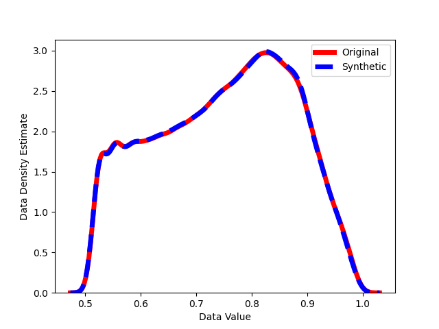
((a))

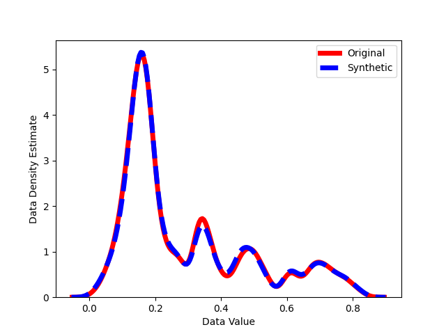
((b))

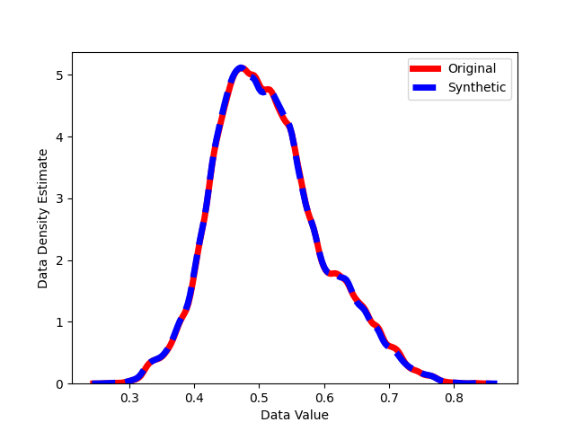
((c))

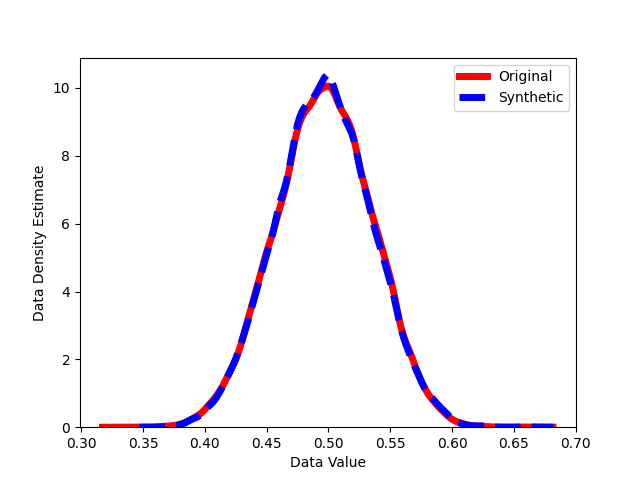
((d))

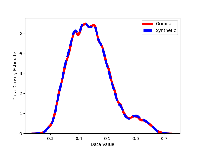
((e))

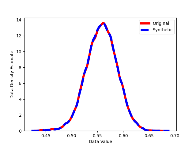
((f))

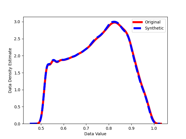
((g))

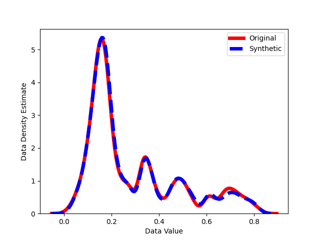
((h))

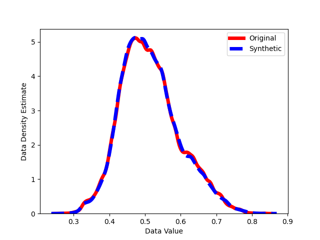
((i))

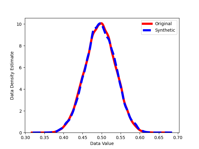
((j))

((k))

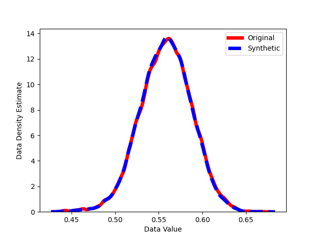
((l))

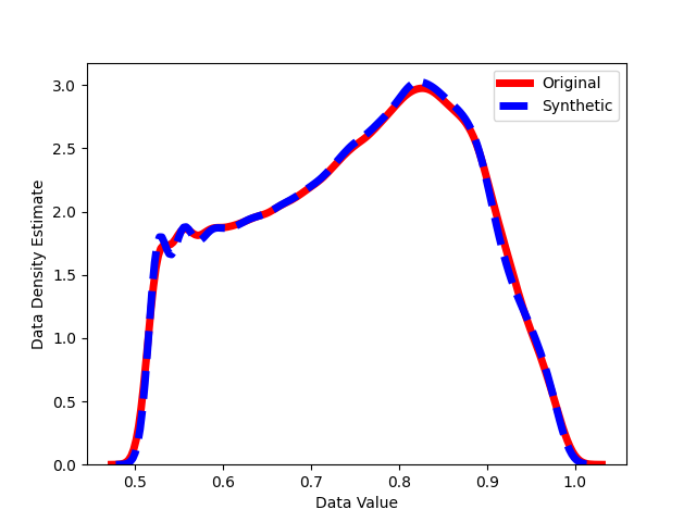
((a))

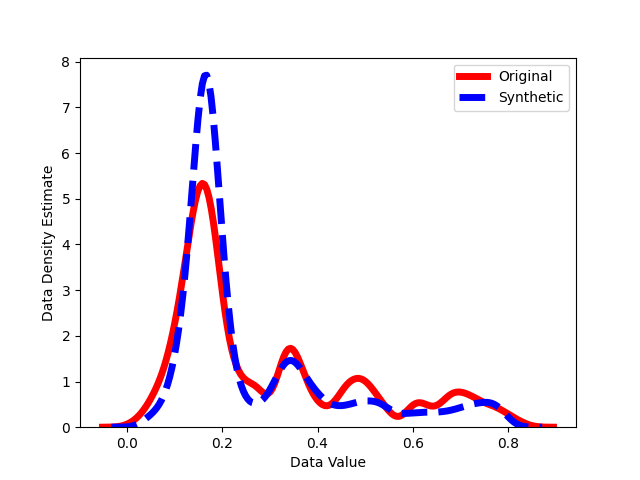
((b))

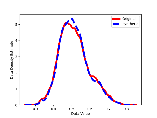
((c))

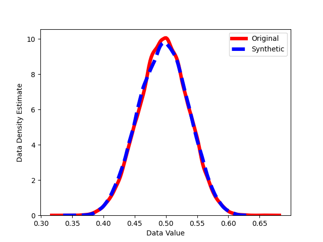
((d))

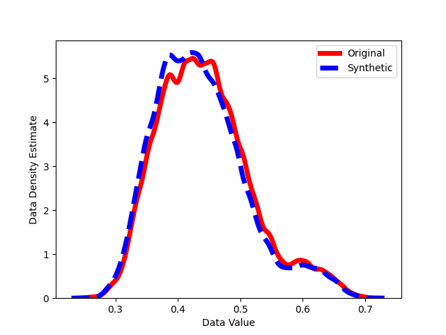
((e))

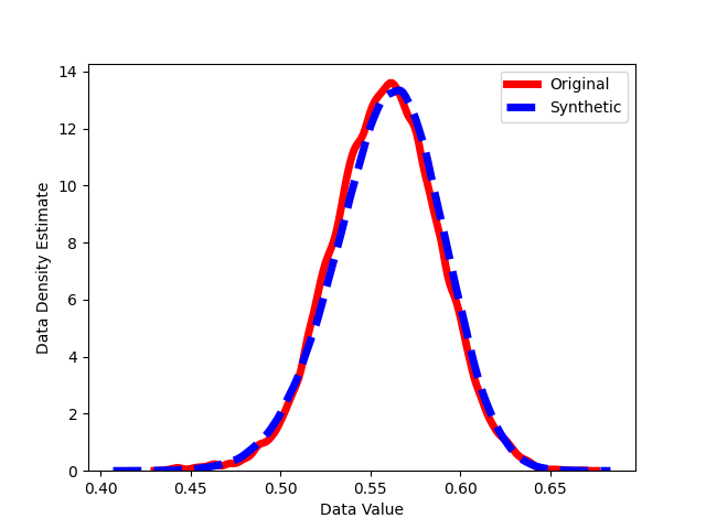
((f))

SDformer

Diffusion-TS

Figure 3: Kernel density estimation visualizations of the time series synthesized by MSDformer, SDformer and Diffusion-TS.

MSDformer

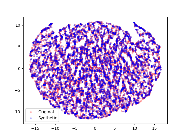
((a))

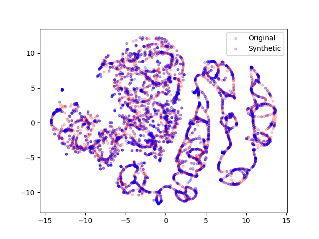
((b))

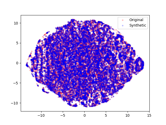
((c))

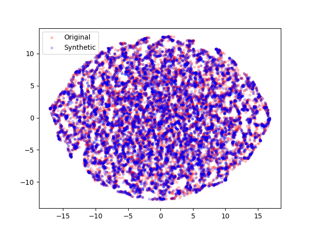
((d))

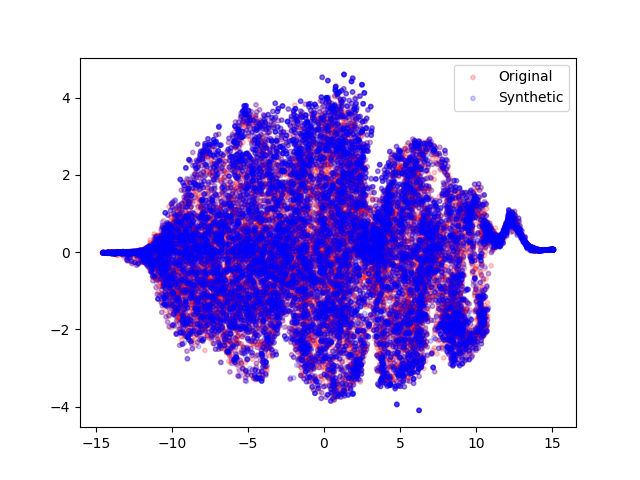
((e))

((f))

((g))

((h))

((i))

((j))

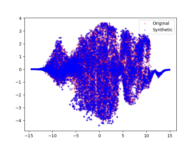
((k))

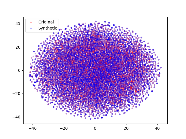
((l))

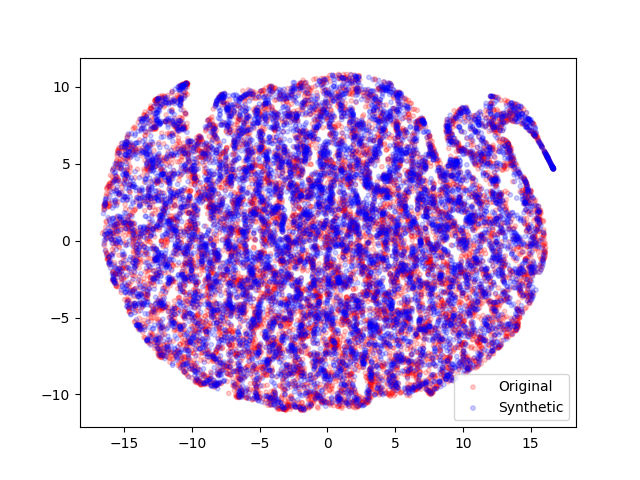
((a))

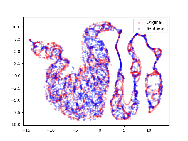
((b))

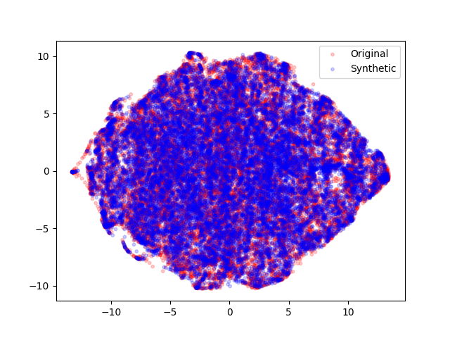
((c))

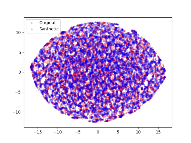
((d))

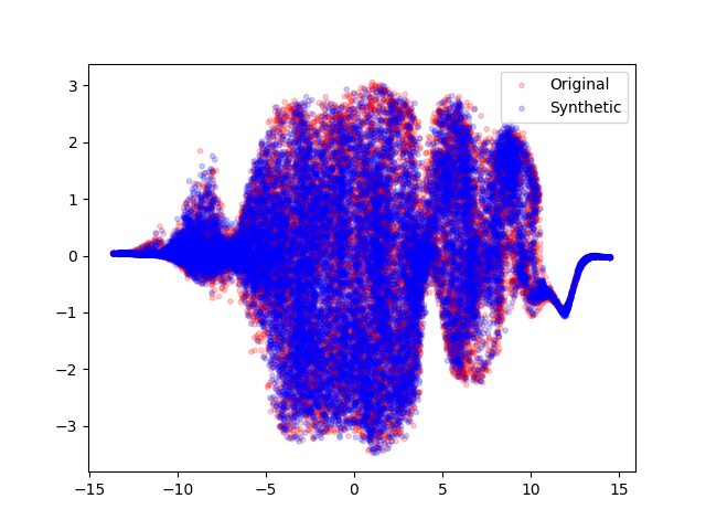
((e))

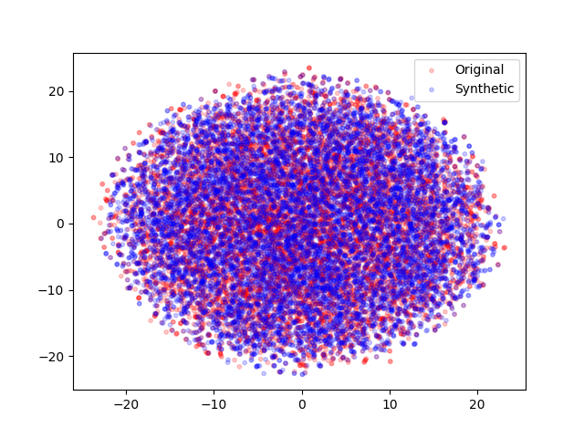
((f))

SDformer

Diffusion-TS

Figure 4: t-SNE visualizations of the time series synthesized by MSDformer, SDformer and Diffusion-TS.

VI-D Efficiency Analysis

TABLE III: Comparison of inference time (per 1024 samples) across methods and datasets.

Methods	Sines	Stocks	ETTh	MuJoCo	Energy	fMRI
Diffusion-TS	9.57	10.12	11.85	19.34	34.92	45.90
SDformer	0.15	0.18	0.40	0.15	0.15	0.44
MSDformer	0.95	0.96	0.30	0.97	0.96	1.40

To validate the practical efficiency of different methods, we compare their inference speeds, as shown in Table III. As can be seen from the table, DTM-based methods, namely SDformer and MSDformer, significantly outperform DDPMs-based methods such as Diffusion-TS in terms of inference speed, with a difference of more than 10 times. This is because DDPMs-based methods require multiple denoising steps, leading to longer inference times. Additionally, MSDformer requires more inference time than SDformer. This is because multi-scale modeling, while learning higher-quality discrete representations of time series, also increases the length of the discrete token sequence, thereby increasing the time required for autoregressive generation. Despite the moderate speed cost, MSDformer’s significant quality gains in both short-term and long-term generation (as shown in Section VI-B and Section VI-C) justify this trade-off for most real-world applications. The choice between SDformer and MSDformer can be adapted to specific latency-vs-quality requirements.

VI-E Ablation Studies

To understand the contribution of each design or component to proposed method, we conduct ablation experiments for six aspects: 1) the effect of increasing codebook size vs. number of scales; 2) the effect of different scale configuration; 3) the effect of similarity-driven vector quantization; 4) the effect of exponential moving average for codebook update; 5) the effect of codebook reset; 6) the effect of token type encoding.

Effect of Increasing Codebook Size vs. Number of Scales. Section V-B demonstrates that increasing the number of scales allows for lower distortion compared to increasing the codebook size. Furthermore, we provide an experimental performance comparison of these approaches under different length settings on the fMRI dataset, as shown in Table IV. From the comparison, it is evident that using SDformer with a codebook size of $V=512$ as the baseline, increasing the codebook size to $V=640$ results in performance improvements. However, the performance enhancement is more pronounced and stable when increasing the number of scales (e.g., $V^{(1:K)}=[128,512]$, i.e., MSDformer). These findings align with the theoretical analysis in Section V-B, collectively validating the advantages of multi-scale modeling.

TABLE IV: Performance comparison of increasing the single-scale codebook size vs. number of scales under varying length settings.

$\tau$	$V^{(1:K)}$	Discriminative Score$\downarrow$	Predictive Score$\downarrow$	Context-FID Score$\downarrow$
$24$	$[512]$	0.017±.007	0.091±.002	0.015±.001
	$[640]$	0.017±.008	0.091±.003	0.013±.000
	$[128,512]$	0.005±.003	0.090±.002	0.009±.001
$64$	$[512]$	0.013±.011	0.083±.003	0.046±.003
	$[640]$	0.011±.005	0.085±.003	0.044±.003
	$[128,512]$	0.009±.005	0.083±.002	0.041±.003

Effect of Different Scale Configuration. Our method’s key innovation over SDformer is the integration of multi-scale modeling. This part analyzes the impact of multi-scale modeling and different scale sizes. Table V summarizes MSDformer’s performance on the fMRI dataset under various scale configurations, highlighting several key points:

Under single-scale settings ($K=1$), optimal temporal downsampling factors vary across datasets. For instance, the fMRI dataset performs best with a downsampling factor of $r=2$, while Stocks is optimal at $r=4$. This reflects the differing importance of information at various scales across datasets. Excessively large downsampling factors, like $r=8$, consistently degrade performance, as seen in the fMRI and Stocks datasets. These factors result in significant performance degradation in both Discriminative Score and Context-FID Score compared to the optimal single-scale configuration.

Multi-scale modeling significantly boosts performance when properly configured. For fMRI dataser, all multi-scale setups ($K\geq 2$) outperform single-scale baselines, particularly in Discriminative Score and Context-FID Score. The configuration $r^{(1:K)}=[2,8]$ excels among single and dual-scale cases, balancing local and global features. The triple-scale setup $r^{(1:K)}=[2,4,8]$ offers stable, robust performance across metrics, confirming the utility of each scale.

For Stocks dataset, only the Discriminative Score consistently improves over single-scale configurations in dual-scale setups, while Context-FID Score does not. The best performance is achieved with $r^{(1:K)}=[2,4]$, as it integrates useful information from both scales. Including $r=8$ does not enhance performance, likely due to limited large-scale information in the dataset.

Thus, increasing the number of scales does not inherently improve performance; it depends on the dataset and data characteristics. Positive gains are only achieved by adding scales that contain useful information.

TABLE V: Ablation Study on the Impact of Multi-Scale Information and Scale Sizes.

			fRMI			Stocks
	$r^{(1:K)}$	Discriminative Score$\downarrow$	Predictive Score$\downarrow$	Context-FID Score$\downarrow$	Discriminative Score$\downarrow$	Predictive Score$\downarrow$	Context-FID Score$\downarrow$
$K=1$	$[2]$	0.017±.007	0.091±.002	0.015±.001	0.013±.006	0.037±.000	0.003±.001
	$[4]$	0.018±.007	0.092±.002	0.011±.001	0.010±.006	0.037±.000	0.002±.000
	$[8]$	0.032±.012	0.093±.002	0.092±.008	0.017±.007	0.037±.000	0.004±.001
$K=2$	$[2,4]$	0.005±.003	0.091±.002	0.009±.001	0.005±.004	0.037±.000	0.002±.000
	$[2,8]$	0.005±.003	0.090±.002	0.009±.000	0.007±.004	0.037±.000	0.002±.000
	$[4,8]$	0.010±.007	0.092±.002	0.010±.000	0.004±.004	0.037±.000	0.003±.000
$K=3$	$[2,4,8]$	0.005±.004	0.089±.003	0.009±.001	0.012±.007	0.037±.001	0.002±.000

Effect of Similarity-Driven Vector Quantization. Vector quantization critically impacts discrete token learning in time series modeling. Following the finding that similarity-driven strategy outperforms distance-based strategy in time series generation tasks [39], we investigate whether MSDformer retains this advantage by replacing its similarity-driven vector quantization with distance-based variant (”w/o similarity” in Table VI). Results show that MSDformer with similarity-driven vector quantization consistently surpasses distance-based counterparts across all metrics, aligning with SDformer’s finding. this superiority stems from the enhanced capacity of similarity metrics to capture directional features (e.g., trends, periodicity), yielding higher-quality discrete representations that better preserve temporal patterns during modeling.

Effect of Exponential Moving Average for Codebook Update. MSDformer employs exponential moving average (EMA) instead of standard gradient-based codebook updates in VQ-VAE [42]. To validate this design, we compare EMA with conventional methods (”w/o EMA” in Table VI denotes gradient-updated variant). Results reveal consistent performance degradation across metrics when using gradient updates, confirming EMA’s critical role. The EMA strategy ensures stable codebook vector updates while preserving long-term temporal patterns through momentum-based optimization, thereby enhancing model stability and representation fidelity.

Effect of Codebook Reset. MSDformer’s codebook reset mechanism reactivates underused vectors to prevent codebook collapse. Ablation experiments show disabling this technique (”w/o Reset” in Table VI) causes severe performance degradation: Discriminative Score rises from 0.005 to 0.423 and Context-FID increases from 0.009 to 14.664. Codebook utilization plummets to 1.1% without reset, indicating most vectors remain inactive during training. This collapse directly limits representational capacity, confirming the reset’s critical role in maintaining codebook diversity through dynamic vector reactivation.

Effect of Token Type Encoding. MSDformer addresses multi-scale feature confusion through Token Type Encoding (TTE). Ablation experiments reveal disabling TTE (”w/o TTE” in Table VI) causes 40% Discriminative Score degradation and 22.2% Context-FID increase, confirming feature entanglement occurs without explicit scale differentiation. This demonstrates TTE’s critical role in maintaining scale-specific feature spaces during multi-scale temporal modeling.

TABLE VI: Results of ablation study.

Methods	Discriminative Score$\downarrow$	Predictive Score$\downarrow$	Context-FID Score$\downarrow$	Codebook Usage$\downarrow$
MSDformer	0.005±.004	0.089±.003	0.009±.001	100%
w/o similarity	0.006±.004	0.092±.002	0.019±.001	100%
w/o EMA	0.007±.004	0.091±.001	0.011±.000	100%
w/o Reset	0.423±.099	0.103±.001	14.664±1.413	1.1%
w/o TTE	0.007±.006	0.090±.002	0.011±.001	100%

VI-F Visual Analysis

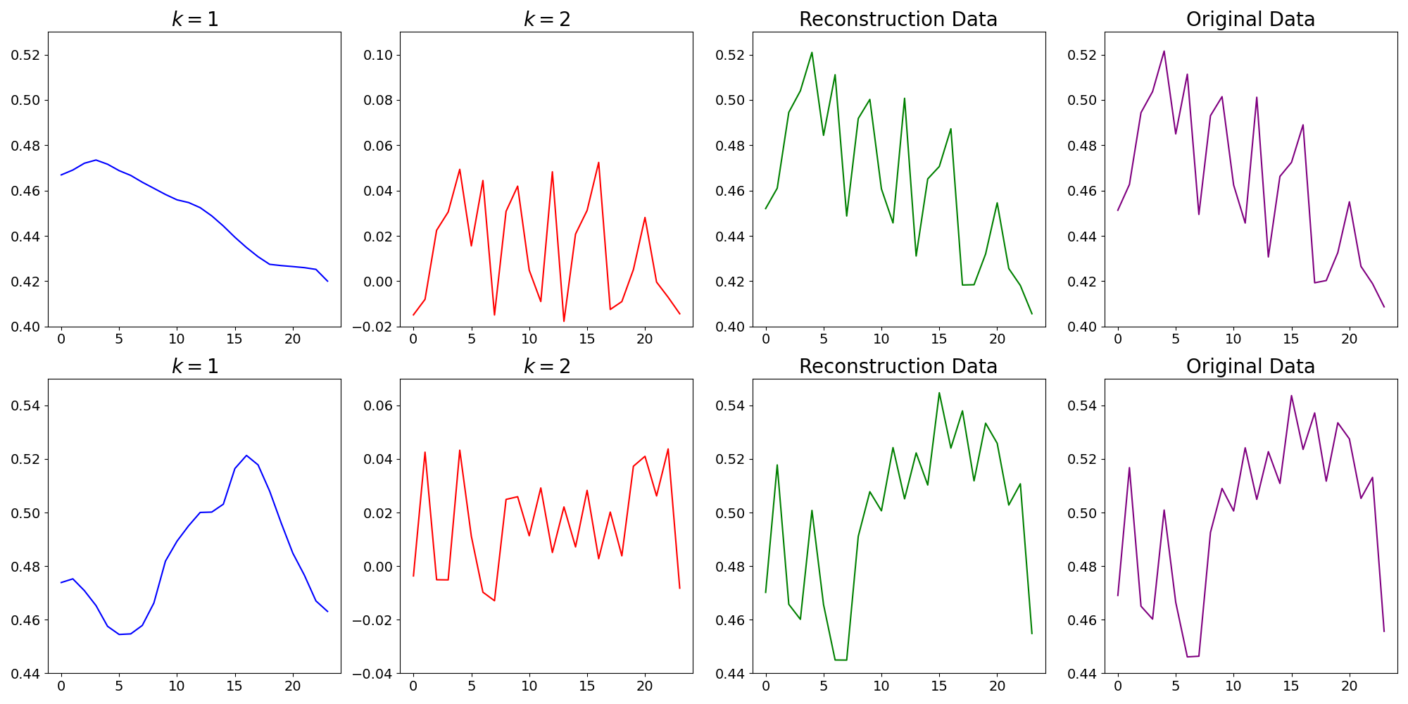
Figure 5: Example of Multi-scale Visualization of Time Series for $K=2$. The first two columns illustrate the multi-scale reconstructions derived from hierarchical representations, specifically showing the coarse-scale reconstruction ($k=1$) and the fine-scale reconstruction ($k=2$). The subsequent two columns display the final reconstruction results and the original data for comparison.

The experimental results demonstrate that incorporating multi-scale information and establishing multi-scale patterns modeling in the DTM-based time series generation framework lead to significant performance improvements. To elucidate the operational mechanism of MSDformer in learning multi-scale temporal features, we conduct a dedicated analysis of the relationship between the original time series and the multi-scale token sequences generated by the multi-scale time series tokenizer.

Specifically, we conduct a controlled experiment using the Energy dataset with $K=2$, corresponding to two distinct scales. After the model converges, component-wise decoding is performed by feeding each scale-specific token sequence into its corresponding decoder module. The reconstructed results for each scale, along with the complete reconstruction and the original time series, are visualized and compared, as shown in Fig. 5.

As illustrated in Fig. 5, the following observations can be made: Firstly, the coarse-scale decoder effectively reconstructs the global trend trajectories and periodic structures, capturing the overall shape and long-term dynamics of the time series. Secondly, the fine-scale decoder focuses on capturing high-frequency signal components and local pattern details, thereby adding finer textures and short-term fluctuations to the reconstruction. Finally, the integrated reconstruction combines both resolution levels, merging the global trends and local details to achieve optimal fidelity. This combined approach ensures that the reconstructed time series closely matches the original data in both structure and detail.

VII Conclusions

This paper introduces a novel DTM-based method, MSDformer, which extends SDformer by incorporating multi-scale modeling, thereby significantly enhancing its ability to handle multi-scale patterns. Additionally, the superiority of the DTM technique in time series generation tasks is demonstrated through the lens of rate-distortion theory. We also provide a theoretical analysis of the advantages of multi-scale modeling. Furthermore, experimental results reveal that DTM-based methods, specifically MSDformer and SDformer, consistently outperform continuous models such as GANs, VAEs, and DDPMs in time series generation (TSG) task. The experiments also highlight the advantages of multi-scale modeling, with MSDformer showing notable improvements over SDformer.

Looking ahead, future work could focus on enhancing scalability by exploring adaptive multi-scale structures that dynamically adjust the number of scales and downsampling rates at different temporal resolutions. The framework could also be extended to more complex scenarios, such as spatiotemporal data generation and multivariate conditional generation, to explore its cross-modal potential. This study not only advances time series generation but also provides valuable insights for other temporal analysis tasks, such as forecasting and anomaly detection.

Supplementary Materials for MSDformer

In the supplementary, we provide more implementation details of our SDformer and MSDformer. We organize our supplementary as follows:

• In Section I, we give the detailed description of used datasets and the metrics.

• In Section II, we provide the experiment settings.

• In Section III, we briefly introduce the baselines.

• In Section IV, we show more experimental results to verify the effect of increasing codebook size vs. number of scales.

• In Section VI, we provide the details operations of the architecture in stage 1 and 2.

• In Section V, we provide the algorithms of training in SDformer and MSDformer.

I Dataset and Metric Details

Dataset. The Stocks dataset consists of Google’s stock price data between 2004 and 2019, with each observation representing a day and containing 6 features. The ETTh dataset includes data obtained from electrical transformers, encompassing load and oil temperature measurements taken every 15 minutes from July 2016 to July 2018. The Energy dataset, a UCI appliance energy prediction dataset, comprises 28 features. The fMRI dataset serves as a benchmark for causal discovery and features realistic simulations of blood-oxygen-level-dependent (BOLD) time series; we chose a simulation with 50 features from the original dataset referring to [26]. The Sines dataset contains 5 features, each generated independently with varying frequencies and phases. The MuJoCo dataset is a multivariate physics simulation time series dataset with 14 features.

Quantitative Metrics. The Discriminative Score measures the distributional similarity between original and synthesized time series data. A binary classifier (e.g., RNN) is trained to distinguish original data (labeled as ”real”) from synthesized data (labeled as ”synthetic”), followed by evaluating its classification accuracy on a test set. The score is derived as the absolute difference between the classifier’s accuracy and the random-guessing baseline (0.5), where a value closer to 0 indicates higher similarity between the two datasets. The Predictive Score evaluates the temporal fidelity of synthesized data by training a forecasting model (e.g., RNN) on synthetic data to predict future time steps and testing its generalization on the original dataset. The score is quantified via the model’s mean absolute error (MAE) on real test samples, where lower values indicate better preservation of the original data’s temporal dynamics. The Context-FID Score evaluates the distributional fidelity of synthesized time series by comparing contextual feature embeddings between original and synthetic datasets. A self-supervised embedding network (e.g., trained via temporal contrastive learning) first extracts context-aware representations from both datasets. The Fréchet distance is then computed between the multivariate Gaussian distributions of these embeddings, characterized by their means and covariance matrices. Lower scores indicate closer alignment in contextual patterns between real and synthetic data.

Qualitative Metric. The t-SNE [52] method projects high-dimensional time series data into 2D space to reveal underlying structural patterns. It first computes pairwise similarities in the original space using adaptive Gaussian kernels (guided by perplexity parameters), then optimizes a low-dimensional t-distribution representation through KL divergence minimization. The final visualization preserves neighborhood relationships while mitigating crowding effects, enabling intuitive comparison of real and synthetic data distributions. The Kernel Density Estimation (KDE) evaluates distribution alignment by estimating probability densities through Gaussian kernel smoothing across multiple dimensions. Using bandwidth-optimized kernels, it generates continuous density profiles for both datasets. Visual comparison of these smoothed distributions reveals preservation of key statistical patterns in synthetic data, with overlapping contours indicating higher fidelity.

II Experimental Settings

In this part, we introduce our main experimental settings. For the time series generation task, we conduct five evaluations to obtain the experimental results. Furthermore, the detailed hyperparameters of SDformer and MSDformer are summarized in Tables VII and VIII, respectively. Parameter counts for both models are provided in Table IX.

TABLE VII: Detailed hyperparameters of SDformer.

Dataset	Sines	Stocks	ETTh	MuJoCo	Energy	fMRI
$V$	1024	512	512	512	512	512
$d_{c}$	512	256	512	512	512	512
$\lambda$	0.5	2.0	0.5	0.5	0.001	0.01
$r$	4	4	4	4	4	2
$N_{enc}$	2	2	2	2	2	1
$N_{trans}$	2	2	6	2	2	2
$\epsilon$	0.3	0.3	0.3	0.1	0.1	0.1

• Number of encoder layers

• Number of transformer layers

TABLE VIII: Detailed hyperparameters of MSDformer.

Dataset	Sines	Stocks	ETTh	MuJoCo	Energy	fMRI
$V^{(1:K)}$	[512,512]	[256,512]	[128,512]	[512,512]	[512,512]	[128,512,512]
$d_{c}$	512	512	512	512	512	512
$\lambda$	1.0	0.5	0.5	1.0	0.0005	0.01
$r^{(1:K)}$	[2,4]	[2,4]	[4,8]	[2,4]	[2,4]	[2,4,8]
$N_{enc}$	[1,2]	[1,2]	[2,3]	[1,2]	[1,2]	[1,2,3]
$N_{trans}$	2	2	2	2	2	2
$\epsilon$	0.1	0.3	0.1	0.1	0.1	0.1

TABLE IX: Parameter counts of SDformer and MSDformer on various Datasets (Unit: Million). Total parameters are calculated from precise values; minor discrepancies in summation are due to rounding.

Methods	Sines			Stocks			ETTh
	Stage1	Stage2	Total	Stage1	Stage2	Total	Stage1	Stage2	Total
SDformer	18.6	27.3	45.9	18.6	25.7	44.4	18.7	76.6	95.3
MSDformer	29.2	27.3	56.5	29.2	26.8	55.9	45.4	26.5	72.0
Methods	MuJoCo			Energy			fMRI
	Stage1	Stage2	Total	Stage1	Stage2	Total	Stage1	Stage2	Total
SDformer	18.7	26.3	44.9	18.7	26.3	45.0	10.6	26.3	36.9
MSDformer	29.2	27.3	56.5	29.3	27.3	56.6	56.3	27.6	83.9

TABLE X: Performance comparison of increasing the single-scale codebook size vs. number of scales under varying length settings.

$\tau$	$V^{(1:K)}$	Discriminative Score$\downarrow$	Predictive Score$\downarrow$	Context-FID Score$\downarrow$
$24$	$[512]$	0.006±.004	0.249±.000	0.003±.000
	$[1024]$	0.005±.004	0.249±.000	0.003±.000
	$[512,512]$	0.005±.003	0.249±.000	0.003±.000
$64$	$[512]$	0.010±.007	0.247±.001	0.031±.002
	$[1024]$	0.010±.005	0.247±.001	0.034±.003
	$[512,512]$	0.009±.006	0.247±.001	0.027±.003
$128$	$[512]$	0.013±.00	0.244±.000	0.036±.002
	$[1024]$	0.010±.008	0.245±.001	0.031±.003
	$[512,512]$	0.007±.008	0.244±.001	0.034±.004
$256$	$[512]$	0.017±.003	0.243±.002	0.041±.003
	$[1024]$	0.011±.005	0.243±.002	0.034±.003
	$[512,512]$	0.010±.011	0.243±.003	0.032±.002

TABLE XI: The detailed architecture of the time serie tokenizer’s encoder. The ellipsis indicates that layers 3 to 5 are repeated, with the number of repetitions increasing by one for each doubling of the downsampling factor of the encoder.

Layer	Function	Descriptions
1	Convolution	input channel=$d$, output channel=D, kernel size=3, stride=1, padding=1
2	ReLU	nn.ReLU()
3	Convolution	input channel=D, output channel=D, kernel size=4, stride=2, padding=1
4	ResNet	input channel=D, depth=3, dilation growth rate=3
5	ReLU	nn.ReLU()
⋮	⋮	⋮
N	Convolution	input channel= $d_{c}$, output channel=H, kernel size=3, stride=1, padding=1

TABLE XII: The detailed architecture of the time serie tokenizer’s decoder. The ellipsis indicates that layers 3 to 5 are repeated, with the number of repetitions increasing by one for each doubling of the downsampling factor of the encoder.

Layer	Function	Descriptions
1	Convolution	input channel=$d_{c}$, output channel=D, kernel size=3, stride=1, padding=1
2	ReLU	nn.ReLU()
3	ResNet	input channel=D, depth=3, dilation growth rate=3
4	ReLU	nn.ReLU()
5	Upsample	nn.Upsample()
6	Convolution	input channel=D, output channel=D, kernel size=3, stride=1, padding=1
⋮	⋮	⋮
N-2	Convolution	input channel=D, output channel=D, kernel size=3, stride=1, padding=1
N-1	ReLU	nn.ReLU()
N	Convolution	input channel=D, output channel=$d$, kernel size=3, stride=1, padding=1

III Baselines

In this part, we briefly introduce the baselines:

TimeGAN [17] is a method that combines Generative Adversarial Networks (GANs) with sequence modeling. It jointly optimizes supervised and unsupervised adversarial losses to learn both the static features and dynamic dependencies of time series data, thereby generating high-quality synthetic time series.

COT-GAN [18] is a GAN-based method that incorporates causal optimal transport theory. It optimizes the distribution matching between generated and real data to produce high-quality synthetic time series.

TimeVAE [22] is a time series generation method based on Variational Autoencoders (VAEs). It enhances model interpretability by incorporating domain-specific temporal patterns (such as polynomial trends and seasonality) and optimizes training efficiency to accurately represent and efficiently synthesize the temporal attributes of the original data.

DiffTime [25] is a time series generation method based on a constrained optimization framework. It combines conditional diffusion models to efficiently generate synthetic time series that meet specific constraints.

DiffWave [24] is an audio synthesis method based on diffusion probabilistic models. The model combines a non-autoregressive structure with bidirectional dilated convolutions to generate high-quality audio in parallel, offering significant advantages in synthesis speed. It also ensures the quality of the generated audio by progressively denoising white noise to produce the target audio waveform.

Diffusion-TS [26] is a method that uses an encoder-decoder Transformer architecture to decouple the seasonality and trend of time series. It leverages diffusion models for high-precision multivariate time series generation. Additionally, the algorithm directly reconstructs samples rather than noise and uses Fourier loss to constrain periodic characteristics, significantly improving the quality and interpretability of the generated time series.

IV Additional experimental results

In this part, we additionally provide an experimental performance comparison between increasing codebook size and number of scales under different length settings on the Energy dataset, as shown in Table X. The results align with the conclusions drawn in the main text: using SDformer with a codebook size of $V=512$ as the baseline, increasing the codebook size to $V=1024$ leads to performance improvements. However, the performance enhancement is more pronounced and stable when increasing the number of scales (e.g., $V^{(1:K)}=[512,512]$, i.e., MSDformer). This further demonstrates the advantages of multi-scale modeling.

TABLE XIII: The detailed architecture of the Autoregressive Transformer block.

Layer	Function	Descriptions
1	Layernorm	nn.LayerNorm()
2	Casual-attention	CasualAttention(q=x, k=x, v=x)
3	Layernorm	nn.LayerNorm()
4	MLP	nn.Linear()
5	ReLU	nn.ReLU()
6	MLP	nn.Linear()

Algorithm 2 Training of multi-scale time series tokenizer.

Input: Time series dataset $D=\{x_{1:\tau}^{i}\}_{i=1}^{n}$
Output: Multi-scale Encoder $\{\mathcal{E}^{(k)}\}_{k=1}^{K}$, multi-scale Decoder $\{\mathcal{D}^{(k)}\}_{k=1}^{K}$ and multi-scale codebooks $\{C^{(k)}\}_{k=1}^{K}$.

1:for $i\leftarrow 1$ to $N_{iter}$ do

2:  Get the $X_{1:\tau}$ $\sim$ $D$;

3:  Initialize residual input $f_{1:\tau}^{(1)}\leftarrow X_{1:\tau}$;

4:  for $k\leftarrow 1$ to $K$ do

5:   Get the $h_{1:L^{(k)}}^{(k)}$ by Equation (2);

6:   Get the $y_{1:L^{(k)}}^{(k)}$ by Equation (3);

7:   Get the $\tilde{h}_{1:L^{(k)}}^{(k)}$ by Equation (4);

8:   Get the $\tilde{f}_{1:\tau}^{(k)}$ by Equation (5);

9:   Get the $f_{1:\tau}^{(k+1)}$ by Equation (6);

10:  end for

11:  Get the $\tilde{x}_{1:\tau}$ by Equation (7);

12:  Compute the training loss $\mathcal{L}$ by Equation (8);

13:  Complete backpropagation process based on $\mathcal{L}$ and update the parameters of $\{\mathcal{E}^{(k)}\}_{k=1}^{K}$ and $\{\mathcal{D}^{(k)}\}_{k=1}^{K}$;

14:  Update the codebook by Equations (9) and (11);

15:end for

16:Return trained $\{\mathcal{E}^{(k)}\}_{k=1}^{K}$, $\{\mathcal{D}^{(k)}\}_{k=1}^{K}$, and $\{C^{(k)}\}_{k=1}^{K}$.

Algorithm 3 Training of multi-scale autoregressive discrete Transformer.

Input: Time series dataset $D=\{x_{1:\tau}^{i}\}_{i=1}^{n}$, optimized multi-scale time series tokenizer.
Output:Multi-scale autoregressive Discrete Transformer $\mathcal{G}_{ms}$.

1:for $i\leftarrow 1$ to $N_{iter}$ do

2:  Feed the $x_{1:\tau}$ to multi-scale time series tokenizer and get $\left\{y^{(1)}_{1:L^{(1)}},\ldots,y^{(k)}_{1:L^{(k)}},\ldots,y^{(K)}_{1:L^{(K)}}\right\}$.

3:  Get the label $y_{1:L}$ by Equations (12) and (13);

4:  Get the input $\tilde{y}_{1:L}^{in}$ by Equations (14) and (15);

5:  Feed the $\tilde{y}_{1:L}^{in}$ to $\mathcal{G}_{ms}$;

6:  Compute the training loss $\mathcal{L}_{ms}$ by Equation (22);

7:  Complete backpropagation process based on $\mathcal{L}_{ms}$ and update the parameters of $\mathcal{G}_{ms}$;

8:end for

9:Return trained $\mathcal{G}_{ms}$.

V Algorithms

In this section, we detail the training algorithms for MSDformer, which consists of two stages. In stage 1, our objective is to train a multi-scale time series tokenizer that can produce high-quality discrete representations of time series data while ensuring excellent reconstruction performance. In stage 2, we aim to train a multi-scale autoregressive discrete Transformer that learns the distribution of multi-scale discrete token sequences, thereby enabling the generation of new time series data. Specifically, Algorithm 2 outlines the training procedure for the multi-scale time series tokenizer in stage 1, while Algorithm 3 elucidates the training processes for the multi-scale autoregressive discrete Transformer in stage 2. The inference algorithm is presented in Algorithm 1 within the main text. For the training algorithms for SDformer, simply set the number of scales $K$ in MSDformer to 1.

VI Model details

In this section, we present the detailed network architecture of SDformer and MSDformer. In Stage 1, MSDformer and SDformer employ identical encoder architectures and identical decoder architectures. The only structural variation arises from differing layer counts in specific modules due to distinct downsampling factors, as documented in Tables XI and XII. In stage 2, the multi-scale autoregressive Discrete Transformer is implemented as a standard decoder-only Transformer, with its block structure depicted in Table XIII.

References

- [1] C. Liu, S. C. Hoi, P. Zhao, and J. Sun, “Online arima algorithms for time series prediction,” in Proceedings of the AAAI conference on artificial intelligence, vol. 30, no. 1, 2016.
- [2] Q. Ding, S. Wu, H. Sun, J. Guo, and J. Guo, “Hierarchical multi-scale gaussian transformer for stock movement prediction.” in IJCAI, 2020, pp. 4640–4646.
- [3] J. Yoo, Y. Soun, Y.-c. Park, and U. Kang, “Accurate multivariate stock movement prediction via data-axis transformer with multi-level contexts,” in Proceedings of the 27th ACM SIGKDD Conference on Knowledge Discovery & Data Mining, 2021, pp. 2037–2045.
- [4] K. Xu, Y. Zhang, D. Ye, P. Zhao, and M. Tan, “Relation-aware transformer for portfolio policy learning,” in Proceedings of the twenty-ninth international conference on international joint conferences on artificial intelligence, 2021, pp. 4647–4653.
- [5] M. Zhang, “Financial time series frequent pattern mining algorithm based on time series arima model,” in 2023 International Conference on Networking, Informatics and Computing (ICNETIC), 2023, pp. 244–247.
- [6] R. B. Penfold and F. Zhang, “Use of interrupted time series analysis in evaluating health care quality improvements,” Academic pediatrics, vol. 13, no. 6, pp. S38–S44, 2013.
- [7] M. Qiu, P. Zhao, K. Zhang, J. Huang, X. Shi, X. Wang, and W. Chu, “A short-term rainfall prediction model using multi-task convolutional neural networks,” in 2017 IEEE international conference on data mining (ICDM). IEEE, 2017, pp. 395–404.
- [8] B. Lim and S. Zohren, “Time-series forecasting with deep learning: a survey,” Philosophical Transactions of the Royal Society A, vol. 379, no. 2194, p. 20200209, 2021.
- [9] S. Feng, C. Miao, K. Xu, J. Wu, P. Wu, Y. Zhang, and P. Zhao, “Multi-scale attention flow for probabilistic time series forecasting,” IEEE Transactions on Knowledge and Data Engineering, 2023.
- [10] S. Feng, C. Miao, Z. Zhang, and P. Zhao, “Latent diffusion transformer for probabilistic time series forecasting,” in Proceedings of the AAAI Conference on Artificial Intelligence, vol. 38, no. 11, 2024, pp. 11 979–11 987.
- [11] B. Lim, S. Ö. Arık, N. Loeff, and T. Pfister, “Temporal fusion transformers for interpretable multi-horizon time series forecasting,” International Journal of Forecasting, vol. 37, no. 4, pp. 1748–1764, 2021.
- [12] T. Zhou, P. Niu, L. Sun, R. Jin et al., “One fits all: Power general time series analysis by pretrained lm,” Advances in neural information processing systems, vol. 36, pp. 43 322–43 355, 2023.
- [13] S. Wu, X. Xiao, Q. Ding, P. Zhao, Y. Wei, and J. Huang, “Adversarial sparse transformer for time series forecasting,” Advances in neural information processing systems, vol. 33, pp. 17 105–17 115, 2020.
- [14] A. Alaa, A. J. Chan, and M. van der Schaar, “Generative time-series modeling with fourier flows,” in International Conference on Learning Representations, 2020.
- [15] O. Mogren, “C-rnn-gan: Continuous recurrent neural networks with adversarial training,” arXiv preprint arXiv:1611.09904, 2016.
- [16] C. Esteban, S. L. Hyland, and G. Rätsch, “Real-valued (medical) time series generation with recurrent conditional gans,” arXiv preprint arXiv:1706.02633, 2017.
- [17] J. Yoon, D. Jarrett, and M. Van der Schaar, “Time-series generative adversarial networks,” Advances in neural information processing systems, vol. 32, 2019.
- [18] T. Xu, L. K. Wenliang, M. Munn, and B. Acciaio, “Cot-gan: Generating sequential data via causal optimal transport,” Advances in neural information processing systems, vol. 33, pp. 8798–8809, 2020.
- [19] H. Pei, K. Ren, Y. Yang, C. Liu, T. Qin, and D. Li, “Towards generating real-world time series data,” in 2021 IEEE International Conference on Data Mining (ICDM). IEEE, 2021, pp. 469–478.
- [20] P. Jeha, M. Bohlke-Schneider, P. Mercado, S. Kapoor, R. S. Nirwan, V. Flunkert, J. Gasthaus, and T. Januschowski, “Psa-gan: Progressive self attention gans for synthetic time series,” in The Tenth International Conference on Learning Representations, 2022.
- [21] J. Jeon, J. Kim, H. Song, S. Cho, and N. Park, “Gt-gan: General purpose time series synthesis with generative adversarial networks,” Advances in Neural Information Processing Systems, vol. 35, pp. 36 999–37 010, 2022.
- [22] A. Desai, C. Freeman, Z. Wang, and I. Beaver, “Timevae: A variational auto-encoder for multivariate time series generation,” arXiv preprint arXiv:2111.08095, 2021.
- [23] I. Naiman, N. B. Erichson, P. Ren, M. W. Mahoney, and O. Azencot, “Generative modeling of regular and irregular time series data via koopman VAEs,” in The Twelfth International Conference on Learning Representations, 2024. [Online]. Available: https://openreview.net/forum?id=eY7sLb0dVF
- [24] Z. Kong, W. Ping, J. Huang, K. Zhao, and B. Catanzaro, “Diffwave: A versatile diffusion model for audio synthesis,” in 9th International Conference on Learning Representations, ICLR 2021, Virtual Event, Austria, May 3-7, 2021.
- [25] A. Coletta, S. Gopalakrishnan, D. Borrajo, and S. Vyetrenko, “On the constrained time-series generation problem,” Advances in Neural Information Processing Systems, vol. 36, 2024.
- [26] X. Yuan and Y. Qiao, “Diffusion-ts: Interpretable diffusion for general time series generation,” arXiv preprint arXiv:2403.01742, 2024.
- [27] J. Achiam, S. Adler, S. Agarwal, L. Ahmad, I. Akkaya, F. L. Aleman, D. Almeida, J. Altenschmidt, S. Altman, S. Anadkat et al., “Gpt-4 technical report,” arXiv preprint arXiv:2303.08774, 2023.
- [28] R. Anil, A. M. Dai, O. Firat, M. Johnson, D. Lepikhin, A. Passos, S. Shakeri, E. Taropa, P. Bailey, Z. Chen et al., “Palm 2 technical report,” arXiv preprint arXiv:2305.10403, 2023.
- [29] A. Ramesh, M. Pavlov, G. Goh, S. Gray, C. Voss, A. Radford, M. Chen, and I. Sutskever, “Zero-shot text-to-image generation,” in International conference on machine learning. Pmlr, 2021, pp. 8821–8831.
- [30] J. Yu, Y. Xu, J. Y. Koh, T. Luong, G. Baid, Z. Wang, V. Vasudevan, A. Ku, Y. Yang, B. K. Ayan, B. Hutchinson, W. Han, Z. Parekh, X. Li, H. Zhang, J. Baldridge, and Y. Wu, “Scaling autoregressive models for content-rich text-to-image generation,” Trans. Mach. Learn. Res., vol. 2022.
- [31] H. Chang, H. Zhang, L. Jiang, C. Liu, and W. T. Freeman, “Maskgit: Masked generative image transformer,” in Proceedings of the IEEE/CVF Conference on Computer Vision and Pattern Recognition, 2022, pp. 11 315–11 325.
- [32] H. Chang, H. Zhang, J. Barber, A. Maschinot, J. Lezama, L. Jiang, M. Yang, K. P. Murphy, W. T. Freeman, M. Rubinstein, Y. Li, and D. Krishnan, “Muse: Text-to-image generation via masked generative transformers,” in International Conference on Machine Learning, ICML 2023, 23-29 July 2023, Honolulu, Hawaii, USA.
- [33] L. Yu, Y. Cheng, K. Sohn, J. Lezama, H. Zhang, H. Chang, A. G. Hauptmann, M.-H. Yang, Y. Hao, I. Essa et al., “Magvit: Masked generative video transformer,” in Proceedings of the IEEE/CVF Conference on Computer Vision and Pattern Recognition, 2023, pp. 10 459–10 469.
- [34] R. Villegas, M. Babaeizadeh, P.-J. Kindermans, H. Moraldo, H. Zhang, M. T. Saffar, S. Castro, J. Kunze, and D. Erhan, “Phenaki: Variable length video generation from open domain textual descriptions,” in International Conference on Learning Representations, 2022.
- [35] D. Kondratyuk, L. Yu, X. Gu, J. Lezama, J. Huang, G. Schindler, R. Hornung, V. Birodkar, J. Yan, M. Chiu, K. Somandepalli, H. Akbari, Y. Alon, Y. Cheng, J. V. Dillon, A. Gupta, M. Hahn, A. Hauth, D. Hendon, A. Martinez, D. Minnen, M. Sirotenko, K. Sohn, X. Yang, H. Adam, M. Yang, I. Essa, H. Wang, D. A. Ross, B. Seybold, and L. Jiang, “Videopoet: A large language model for zero-shot video generation,” in Forty-first International Conference on Machine Learning, ICML 2024, Vienna, Austria, July 21-27, 2024, 2024.
- [36] N. Zeghidour, A. Luebs, A. Omran, J. Skoglund, and M. Tagliasacchi, “Soundstream: An end-to-end neural audio codec,” IEEE/ACM Transactions on Audio, Speech, and Language Processing, vol. 30, pp. 495–507, 2021.
- [37] J. Copet, F. Kreuk, I. Gat, T. Remez, D. Kant, G. Synnaeve, Y. Adi, and A. Défossez, “Simple and controllable music generation,” Advances in Neural Information Processing Systems, vol. 36, pp. 47 704–47 720, 2023.
- [38] S. Chen, C. Wang, Y. Wu, Z. Zhang, L. Zhou, S. Liu, Z. Chen, Y. Liu, H. Wang, J. Li et al., “Neural codec language models are zero-shot text to speech synthesizers,” IEEE Transactions on Audio, Speech and Language Processing, 2025.
- [39] C. Zhicheng, F. SHIBO, Z. Zhang, X. Xiao, X. Gao, and P. Zhao, “Sdformer: Similarity-driven discrete transformer for time series generation,” in The Thirty-eighth Annual Conference on Neural Information Processing Systems, 2024.
- [40] F. Shibo, P. Zhao, L. Liu, P. Wu, and Z. Shen, “Hdt: Hierarchical discrete transformer for multivariate time series forecasting,” in Proceedings of the AAAI Conference on Artificial Intelligence, vol. 39, no. 1, 2025, pp. 746–754.
- [41] J. Pang, W. Sun, J. S. Ren, C. Yang, and Q. Yan, “Cascade residual learning: A two-stage convolutional neural network for stereo matching,” in Proceedings of the IEEE international conference on computer vision workshops, 2017, pp. 887–895.
- [42] A. Van Den Oord, O. Vinyals et al., “Neural discrete representation learning,” Advances in neural information processing systems, vol. 30, 2017.
- [43] J. Ho, A. Jain, and P. Abbeel, “Denoising diffusion probabilistic models,” Advances in neural information processing systems, vol. 33, pp. 6840–6851, 2020.
- [44] P. Esser, R. Rombach, and B. Ommer, “Taming transformers for high-resolution image synthesis,” in Proceedings of the IEEE/CVF conference on computer vision and pattern recognition, 2021, pp. 12 873–12 883.
- [45] J. Zhang, Y. Zhang, X. Cun, S. Huang, Y. Zhang, H. Zhao, H. Lu, and X. Shen, “T2m-gpt: Generating human motion from textual descriptions with discrete representations,” arXiv preprint arXiv:2301.06052, 2023.
- [46] B. Jiang, X. Chen, W. Liu, J. Yu, G. Yu, and T. Chen, “Motiongpt: Human motion as a foreign language,” Advances in Neural Information Processing Systems, vol. 36, 2024.
- [47] J. Devlin, M. Chang, K. Lee, and K. Toutanova, “BERT: pre-training of deep bidirectional transformers for language understanding,” in Proceedings of the 2019 Conference of the North American Chapter of the Association for Computational Linguistics: Human Language Technologies, NAACL-HLT 2019, Minneapolis, MN, USA, June 2-7, 2019, Volume 1 (Long and Short Papers), 2019.
- [48] K. Tian, Y. Jiang, Z. Yuan, B. Peng, and L. Wang, “Visual autoregressive modeling: Scalable image generation via next-scale prediction,” Advances in neural information processing systems, vol. 37, pp. 84 839–84 865, 2024.
- [49] W. Williams, S. Ringer, T. Ash, D. MacLeod, J. Dougherty, and J. Hughes, “Hierarchical quantized autoencoders,” Advances in Neural Information Processing Systems, vol. 33, pp. 4524–4535, 2020.
- [50] A. Vaswani, N. Shazeer, N. Parmar, J. Uszkoreit, L. Jones, A. N. Gomez, Ł. Kaiser, and I. Polosukhin, “Attention is all you need,” Advances in neural information processing systems, vol. 30, 2017.
- [51] C. E. Shannon, “Coding theorems for a discrete source with a fidelity criterion,” IRE International Convention Record, vol. 7, no. 4, pp. 142–163, 1959.
- [52] L. Van der Maaten and G. Hinton, “Visualizing data using t-sne.” Journal of machine learning research, vol. 9, no. 11, 2008.